Implied and Realized Volatility: A Study of the Ratio Distribution

Abstract

We analyze correlations between squared volatility indices, VIX and VXO, and realized variances – the known one, for the current month, and the predicted one, for the following month. We show that the ratio of the two is best fitted by a Beta Prime distribution, whose shape parameters depend strongly on which of the two months is used.

1 Introduction

In a previous study [1], we introduced the ratio of realized variance to implied variance, represented by squared volatility indices VIX or VXO, as a measure of their correlations. We pointed out that the realized variance is calculated for trading dates while the implied variance covers every day, so one of them needs rescaled for a proper comparison. We argued that studying the distribution of the ratios produces a deeper insight into these correlations than a simple regression analysis [2], which arrives at an obvious conclusion that VIX/VXO are a slightly better predictor of the future realized volatility (RV) than the past RV since it builds on the latter with the benefit of additional information.

In [1] we concluded that the ratio of the actual realized variance $RV^{2}$ to $VIX^{2}$ and $VXO^{2}$, that is to its predicted values, was best described by the fat-tailed inverse Gamma (IGa) distribution and its inverse by the Gamma (Ga) distribution.We speculated that this is due to unanticipated spikes of realized volatility. In this paper we show that a Beta Prime (BP) distribution provides a better fit both for the ratio and its inverse. For the former, the exponent of the power dependence for small values of the ratio is very large, which mimics exponential behavior of IGa. For the latter, the exponent of the power-law tails is very large, which mimics exponential decay of Ga.

We also concluded in [1] that the ratio of $RV^{2}$ of the preceding month to $VIX^{2}$ and $VXO^{2}$ was best described by the lognormal (LN) distribution. Its inverse was also best described by the LN with similar parameters. We argued that while the spikes in the past realized volatility lead to spikes of implied volatility, there was enough uncertainty for the ratio to have heavy tails. In this paper we show that BP, with similar parameters for the ratio and its inverse, provides a better fit for both. The exponents of the power law for both small values and the fat tails are large, so that BP mimics the LN behavior. Additionally, for both BP and LN the distribution of the inverse variable is BP and LN respectively as well.

As a reminder to the reader, PDF of BP distribution is given by

$$BP(p,q,\beta;x)=\frac{(1+\frac{x}{\beta})^{-p-q}(\frac{x}{\beta})^{p-1}}{\beta B[p,q]}$$ (1)

where $\beta$ is a scale parameter, $p$ and $q$ are shape parameters and $B[p,q]$ is the Beta function; $BP\propto x^{p-1}$ for $x\ll\beta$ and $BP\propto x^{-q-1}$ for $x\gg\beta$.

This paper is organized as follows. In Section 2 we summarize empirical observations regarding distributions of $RV^{2}$ and volatility indices $VIX^{2}$ and $VXO^{2}$ and their ratios. In Section 3 we show the results of statistical fits of the ratios. In Section 4 we summarize correlations between the quantities and their ratios.

2 Empirical Observations

In [1] we presented empirical distributions (PDF) of $RV^{2}$ vis-a-vis $VIX^{2}$ and $VXO^{2}$, as well as the ratios, and in [3] we will have described their fits. We observe the following features, in agreement with [4] (see also [5, 6]):

• $VIX^{2}$ and $VXO^{2}$ have lower high-volatility probabilities relative to $RV^{2}$, including shorter fat tails, indicating that volatility indices do not predict accurately large values of RV, including the largest volatility spikes. In other word, volatility indices underestimate future large RV.

• $VIX^{2}$ and $VXO^{2}$ have higher mid-volatility probabilities relative to $RV^{2}$, indicating that volatility indices overestimate future mid-level RV.

• $VIX^{2}$ and $VXO^{2}$ have lower low-volatility probabilities relative to $RV^{2}$, indicating that volatility indices underestimate future low RV.

For the distributions of the ratios $RV^{2}/VIX^{2}$, $RV^{2}/VXO^{2}$, it is important to notice that, since realized and implied volatilities are correlated, we cannot construct them simply as the quotient distributions of two independent variable. We observe the following:

2.1 Predicted Month

For the month predicted by the volatility indices

• The distributions have fat tails, indicating again that VIX and VXO underestimate future values of RV, in particular volatility spikes.

• Very small ratios are suppressed, as manifested by a very large power exponent, indicating that it is rare that RV is considerably smaller than the one predicted by the volatility indices.

• The tail exponents of the ratio distributions is larger than that of either $RV^{2}$ or $VIX^{2}$ and $VXO^{2}$, pointing to that for the $RV^{2}$ values taken from the tails, the values of $VIX^{2}$, $VXO^{2}$ are also more likely to come from the tails.

2.2 Preeceding Month

For RV of the preceding month:

• The tails of the distributions are much shorter than those for the predicted month, reflecting the fact that volatility indices account for past RV.

• The tail exponents of the distributions are almost identical to those of their inverse, $VIX^{2}/RV^{2}$ and $VXO^{2}/RV^{2}$ distributions, indicating, as above, strong correlations.

For the ratio distribution of $RV^{2}$ of the predicted (next) month to $RV^{2}$ of the preceding month (see below), we observe that

• The exponent of the fat tail is smaller than those of the $RV^{2}/VIX^{2}$ and $RV^{2}/VXO^{2}$ distributions, that is the tails are longer.

• The power-law exponent at very small ratios is much smaller for this distribution than for $RV^{2}/VIX^{2}$ and $RV^{2}/VXO^{2}$, that is those ratios are far less suppressed.

By both measures, VIX and VXO are better predictors of the future RV than the past RV.

3 Statistical Fits of Ratio Distributions

Below, figures show the plots of the ratios and their distribution fits and tables contain parameters of the distribution and KS statistics. The two novel elements here, relative to [1], is the inclusion of BP in the fits of $RV^{2}/VIX^{2}$ and $RV^{2}/VXO^{2}$ distributions and the fits of the ratio distribution of $RV^{2}$ of the predicted (next) month to $RV^{2}$ of the preceding month (and its inverse).

3.1 Predicted Month

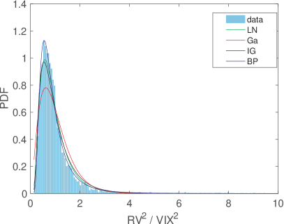
Figure 1: $\mathrm{RV}^{2}/\mathrm{VIX}^{2}$, from Jan 2nd, 1990 to Dec 30th, 2016.

Figure 2: $\mathrm{VIX}^{2}/\mathrm{RV}^{2}$, from Jan 2nd, 1990 to Dec 30th, 2016.

Table 1: MLE results for “$\mathrm{RV}^{2}/\mathrm{VIX}^{2}$” and “$\mathrm{VIX}^{2}/\mathrm{RV}^{2}$”

	parameters	KS test
Normal	N( 1.0000, 0.9067)	0.1940
LogNormal	LN( -0.2027, 0.5867)	0.0446
IGa	IGa( 3.3595, 2.3466)	0.0246
Gamma	Gamma( 2.6219, 0.3814)	0.0978
Weibull	Weibul( 1.1124, 1.4009)	0.1224
IG	IG( 1.0000, 2.3168)	0.0607
BP	BP( 27.2279, 3.8055, 0.1014)	0.0198

	parameters	KS test
Normal	N( 1.0000, 0.5626)	0.0972
LogNormal	LN( -0.1562, 0.5867)	0.0446
IGa	IGa( 2.6219, 1.8314)	0.0978
Gamma	Gamma( 3.3595, 0.2977)	0.0246
Weibull	Weibul( 1.1306, 1.8882)	0.0500
IG	IG( 1.0000, 2.3168)	0.0734
BP	BP( 3.8055, 27.2279, 6.8913)	0.0198

Figure 3: $\mathrm{RV}^{2}/\mathrm{VXO}^{2}$, Jan 2nd, 1990 to Dec 30th, 2016.

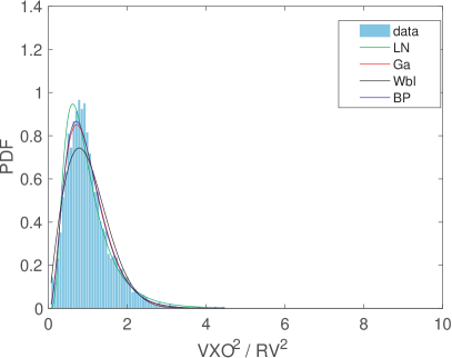
Figure 4: $\mathrm{VXO}^{2}/\mathrm{RV}^{2}$, from Jan 2nd, 1990 to Dec 30th, 2016

Table 2: MLE results for “$\mathrm{RV}^{2}/\mathrm{VXO}^{2}$” and “$\mathrm{VXO}^{2}/\mathrm{RV}^{2}$”

	parameters	KS test
Normal	N( 1.0000, 0.8747)	0.1910
LogNormal	LN( -0.1973, 0.5795)	0.0449
IGa	IGa( 3.4629, 2.4438)	0.0224
Gamma	Gamma( 2.6897, 0.3718)	0.0971
Weibull	Weibul( 1.1150, 1.4256)	0.1230
IG	IG( 1.0000, 2.3981)	0.0611
BP	BP( 47.6001, 3.7157, 0.0563)	0.0177

	parameters	KS test
Normal	N( 1.0000, 0.5467)	0.0925
LogNormal	LN( -0.1513, 0.5795)	0.0449
IGa	IGa( 2.6897, 1.8982)	0.0971
Gamma	Gamma( 3.4629, 0.2888)	0.0224
Weibull	Weibul( 1.1308, 1.9374)	0.0499
IG	IG( 1.0000, 2.3981)	0.0729
BP	BP( 3.7157, 47.6002, 12.5409)	0.0177

3.2 Preceding Month

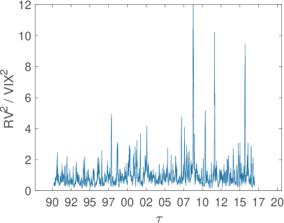
Figure 5: $\mathrm{RV}^{2}/\mathrm{VIX}^{2}$, from Jan 2nd, 1990 to Dec 30th, 2016.

Figure 6: $\mathrm{VIX}^{2}/\mathrm{RV}^{2}$, from Jan 2nd, 1990 to Dec 30th, 2016.

Table 3: MLE results for “$\mathrm{RV}^{2}/\mathrm{VIX}^{2}$” and “$\mathrm{VIX}^{2}/\mathrm{RV}^{2}$”

	parameters	KS test
Normal	N( 1.0000, 0.4974)	0.0992
LogNormal	LN( -0.1099, 0.4689)	0.0147
IGa	IGa( 4.6889, 3.7619)	0.0431
Gamma	Gamma( 4.7110, 0.2123)	0.0381
Weibull	Weibul( 1.1325, 2.1250)	0.0672
IG	IG( 1.0000, 4.0580)	0.0215
BP	BP( 9.2230, 9.9855, 0.9742)	0.0117

	parameters	KS test
Normal	N( 1.0000, 0.4999)	0.1059
LogNormal	LN( -0.1104, 0.4689)	0.0147
IGa	IGa( 4.7110, 3.7796)	0.0381
Gamma	Gamma( 4.6889, 0.2133)	0.0431
Weibull	Weibul( 1.1329, 2.1186)	0.0751
IG	IG( 1.0000, 4.0580)	0.0163
BP	BP( 9.9855, 9.2230, 0.8236)	0.0117

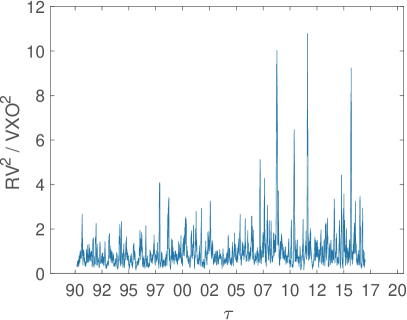
Figure 7: $\mathrm{RV}^{2}/\mathrm{VXO}^{2}$, Jan 2nd, 1990 to Dec 30th, 2016.

Figure 8: $\mathrm{VXO}^{2}/\mathrm{RV}^{2}$, from Jan 2nd, 1990 to Dec 30th, 2016

Table 4: MLE results for “$\mathrm{RV}^{2}/\mathrm{VXO}^{2}$” and “$\mathrm{VXO}^{2}/\mathrm{RV}^{2}$”

	parameters	KS test
Normal	N( 1.0000, 0.4915)	0.1064
LogNormal	LN( -0.1041, 0.4539)	0.0150
IGa	IGa( 5.0351, 4.0948)	0.0331
Gamma	Gamma( 4.9618, 0.2015)	0.0454
Weibull	Weibul( 1.1316, 2.1383)	0.0730
IG	IG( 1.0000, 4.3548)	0.0203
BP	BP( 11.1694, 9.4027, 0.7520)	0.0133

	parameters	KS test
Normal	N( 1.0000, 0.4768)	0.0933
LogNormal	LN( -0.1026, 0.4539)	0.0150
IGa	IGa( 4.9618, 4.0352)	0.0454
Gamma	Gamma( 5.0351, 0.1986)	0.0331
Weibull	Weibul( 1.1319, 2.2099)	0.0689
IG	IG( 1.0000, 4.3548)	0.0212
BP	BP( 9.4027, 11.1694, 1.0814)	0.0133

3.3 Ratio of Realized Variances of Two Adjacent Months

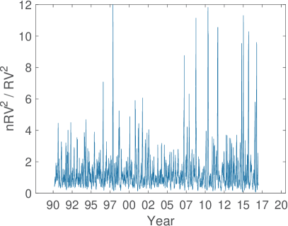
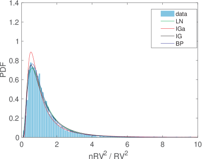
Figure 9: Ratio of next-month realized variance to that of the preceding month, from Jan 2nd, 1990 to Dec 30th, 2016.

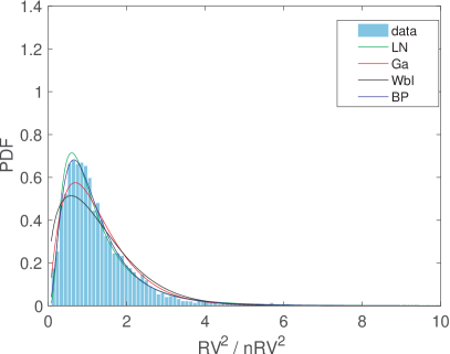
Figure 10: Ratio of preceding-month realized variance to that of the following month, from Jan 2nd, 1990 to Dec 30th, 2016.

Table 5: MLE results for “$\mathrm{nRV}^{2}/\mathrm{RV}^{2}$” and “$\mathrm{RV}^{2}/\mathrm{nRV}^{2}$”

	parameters	KS test
Normal	N( 1.3175, 1.2580)	0.1809
LogNormal	LN( -0.0037, 0.7211)	0.0244
IGa	IGa( 2.1291, 1.6472)	0.0472
Gamma	Gamma( 1.9390, 0.6795)	0.0801
Weibull	Weibul( 1.4403, 1.2869)	0.0922
IG	IG( 1.3175, 1.8743)	0.0340
BP	BP( 5.8771, 3.4893, 0.5556)	0.0123

	parameters	KS test
Normal	N( 1.2925, 1.0777)	0.1422
LogNormal	LN( 0.0037, 0.7211)	0.0244
IGa	IGa( 1.9390, 1.4717)	0.0801
Gamma	Gamma( 2.1291, 0.6071)	0.0472
Weibull	Weibul( 1.4300, 1.3951)	0.0608
IG	IG( 1.2925, 1.8387)	0.0513
BP	BP( 3.4893, 5.8771, 1.7999)	0.0123

4 Correlation Analysis

Tables 6 and 7 list Pearson correlation coefficients (PCC). Here ”n” labels the ”next” month, that is the month for which VIX and VXO were predicting the implied RV; ”r” a ”random” month and unlabeled RV is the one of the preceding month. All $RV^{2}$ are scaled, as explained earlier and in [1]. Tables 8 and 9 list Kolmogorov-Smirnov (KS) statistic for comparison of the two plots.

Table 6: PCC VIX

	$RV^{2}$	$nRV^{2}$	$VIX^{2}$	$rRV^{2}$
$RV^{2}$	1	0.70	0.88	0.0055
$nRV^{2}$	0.70	1	0.71	0.0025
$VIX^{2}$	0.88	0.71	1	0.003
$rRV^{2}$	0.0055	0.0025	0.003	1

Table 7: PCC VXO

	$RV^{2}$	$nRV^{2}$	$VXO^{2}$	$rRV^{2}$
$RV^{2}$	1	0.70	0.87	0.0015
$nRV^{2}$	0.70	1	0.72	0.004
$VXO^{2}$	0.87	0.72	1	0.002
$rRV^{2}$	0.0015	0.004	0.002	1

Table 8: KS VIX

	$\frac{RV^{2}}{VIX^{2}}$	$\frac{nRV^{2}}{VIX^{2}}$	$\frac{RV^{2}}{nRV^{2}}$	$\frac{rRV^{2}}{rVIX^{2}}$	$\frac{rRV^{2}}{rRV^{2}}$	$\frac{nRV^{2}}{RV^{2}}$
$\frac{RV^{2}}{VIX^{2}}$	0	0.056	0.13	0.20	0.26	-
$\frac{nRV^{2}}{VIX^{2}}$	0.056	0	-	0.18	0.23	0.13
$\frac{RV^{2}}{nRV^{2}}$	0.13	-	0	0.17	0.15	-
$\frac{rRV^{2}}{rVIX^{2}}$	0.20	0.18	0.17	0	0.063	0.17
$\frac{rRV^{2}}{rRV^{2}}$	0.26	0.23	0.15	0.063	0	0.16
$\frac{nRV^{2}}{RV^{2}}$	-	0.13	-	0.17	0.16	0

Table 9: KS VXO

	$\frac{RV^{2}}{VXO^{2}}$	$\frac{nRV^{2}}{VXO^{2}}$	$\frac{RV^{2}}{nRV^{2}}$	$\frac{rRV^{2}}{rVXO^{2}}$	$\frac{rRV^{2}}{rRV^{2}}$	$\frac{nRV^{2}}{RV^{2}}$
$\frac{RV^{2}}{VXO^{2}}$	0	0.063	0.13	0.22	0.26	-
$\frac{nRV^{2}}{VXO^{2}}$	0.063	0	-	0.19	0.23	0.16
$\frac{RV^{2}}{nRV^{2}}$	0.13	-	0	0.17	0.16	-
$\frac{rRV^{2}}{rVXO^{2}}$	0.22	0.19	0.17	0	0.057	0.18
$\frac{rRV^{2}}{rRV^{2}}$	0.26	0.23	0.16	0.057	0	0.17
$\frac{nRV^{2}}{RV^{2}}$	-	0.16	-	0.18	0.17	0

5 Conclusions

Beta Prime distribution provides the best fit to the distributions of ratios of realized variance (squared realized volatility) to squared implied volatility indices VIX and VXO, as well as of ratio of realized variances of two consecutive months.

For realized variance of the month for which volatility indices calculate implied realized variance, distributions have very slowly decaying fat tails. This indicates that volatility indices tends to underestimate future volatility, especially its large spikes. Conversely, probability of having very small ratios is suppressed due to a large power-law exponent. Comparing this to the ratio of realized variance of the preceding month to the following month, the latter has even longer tails, while the small ratios are significantly more populated. By both measures, VIX and VXO are better predictors of future realized volatility.

For realized variance of the preceding month, the power law exponents for small ratios and for those in the tails are nearly identical, which reflects the fact that distributions of the ratio and its inverse are nearly identical and that the distribution of the inverse variable of Beta Prime is also Beta Prime.

Correlation and Kolmogorov-Smirnov statistics are in excellent agreement with empirical analysis of Section 2 and fitting in Section 3. In a future work we will more closely identify the months whose ratios are responsible for the tails and the low-ratio regions.

References

- [1] M. Dashti Moghaddam, Z. Liu, R. Serota, Distributions of historic market data – implied and realized volatility, arXiv 1804.05279.
- [2] B. J. Chrstensen, N. R. Prabhala, The relation between implied and realized volaility, Journal of Financial Economics 50 (1998) 125–150.
- [3] M. Dashti Moghaddam, Z. Liu, R. Serota, Realized versus implied volatility and their distributions, to be submitted to arXiv.
- [4] M. D. Russon, A. F. Vakil, On the non-linear relationship between vix and realized sp500 volatility, Investment Management and Financial Innovations 14 (2) (2017) 200–206.
- [5] I. Vodenska, W. J. Chambers, Understanding the relationship between vix and the s&p 500 index volatility, 26th Australasian Finance and Banking Conference (2013).
- [6] C. Kownatzki, How good is the vix as a predictor of market risk?, Journal of Accounting and Finance 16 (6) (2016) 39–60.