Explaining the asymmetric line profile in Cepheus X-4 with spectral variation across pulse phase

Abstract

The high mass X-ray binary Cep X-4, during its 2014 outburst, showed evidence for an asymmetric cyclotron line in its hard X-ray spectrum. The 2014 spectrum provides one of the clearest cases of an asymmetric line profile among all studied sources with Cyclotron Resonance Scattering Features (CRSF). We present a phase-resolved analysis of NuSTAR and Suzaku data taken at the peak and during the decline phases of this outburst. We find that the pulse-phased resolved spectra are well-fit by a single, symmetric cyclotron feature. The fit parameters vary strongly with pulse phase: most notably the central energy and depth of the cyclotron feature, the slope of the power-law component, and the absorbing column density. We synthesise a “phase averaged” spectrum using the best-fit parameters for these individual pulse phases, and find that this combined model spectrum has a similar asymmetry in the cyclotron features as discovered in phase-averaged data. We conclude that the pulse phase resolved analysis with simple symmetric line profiles when combined can explain the asymmetry detected in the phase-averaged data.

1 Introduction

High Mass X-ray Binaries (HMXBs) are systems containing a compact object — either a neutron star (NS) or a black hole — gravitationally bound to a massive, early type star (M $>\ 5$ $M_{\odot}$). In accreting NS HMXBs, the high magnetic field ($\gtrsim 10^{12}$ G) of the NS channels the accreted matter onto the magnetic poles (Mukherjee et al., 2013, and references therein). The kinetic energy of the accreted matter is converted to X-rays near the surface of the NS. X-ray spectroscopy thus allows us to probe regions close to the neutron star. Of particular interest is the effect of the magnetic field on the X-ray spectrum. Resonant scattering of X-ray photons off electrons occupying and transitioning between quantised Landau levels creates Cyclotron Resonant Scattering Features (CRSFs) in the X-ray spectra. The central energy of these features relates directly to the local magnetic field as $E_{\rm cyc}=11.6~{}B_{12}(1+z)^{-1}$ keV, where $B_{12}$ is magnetic field in units of $10^{12}$ G and $z$ is the gravitational redshift.

CRSFs have been observed in several NS HMXBs (see for example Caballero & Wilms, 2012; Mukherjee et al., 2013; Jaisawal & Naik, 2017). These cyclotron features and their harmonics, if any, are usually modelled with a Gaussian optical depth line gabs or with the psuedo-Lorentzian profile cyclabs phenomenological model (Mihara et al., 1990; Makishima et al., 1990). The asymmetric profiles give hints towards the viewing angle onto the magnetic field and the field configuration (see Schwarm et al., 2017a, b). While theoretical work has been done on the expected complex shapes of these features (Mukherjee & Bhattacharya, 2012; Mukherjee et al., 2013; Schwarm et al., 2017a, b, and references therein), further studies have been limited by the energy resolution and sensitivity of X-ray telescopes. Due to excellent spectral resolution of NuSTAR (0.4 keV at 10 keV, Harrison et al., 2013), the shapes of CRSFs can be probed by NuSTAR.

The HMXB Cepheus X-4 (hereafter Cep X-4) was discovered in outburst in 1972 by the OSO-7 satellite (Ulmer et al., 1973). Further studies of a 1988 observation led to the discovery of 66.3 s pulsations (Koyama et al., 1991) and identification of the optical B[e] companion (Roche et al., 1997; Bonnet-Bidaud & Mouchet, 1998). Wilson et al. (1999) used the outbursts seen by BATSE and RXTE in 1993 and 1997 to constrain the orbital period to be between 23 and 147.3 days. McBride et al. (2007) used long term RXTE-ASM lightcurve to constrain the orbital period of Cep X-4 to $20.85\pm 0.05$ days. Mihara et al. (1991) reported the first detection of the cyclotron feature at $30.5\pm 0.4$ keV in Cep X-4, which was confirmed by McBride et al. (2007) with RXTE observations of the 2002 outburst. Detailed NuSTAR observations by Fürst et al. (2015) (hereafter FF15) during the 2014 outburst of Cep X-4 provided clear evidence of an asymmetric CRSF profile in the phase-averaged spectrum, which we explore further in this work. Schwarm et al. (2017b) successfully described the asymmetric line profile observed with NuSTAR at the peak of this outburst with their physical model based on Monte Carlo modelling of CRSFs. Analyses by Jaisawal & Naik (2015) of a lower flux Suzaku observation of this outburst and by Vybornov et al. (2017) of the NuSTAR observations led to the discovery of a harmonic CRSF with an energy ratio to the fundamental line of 1:1.7 and 1.8, respectively.

As the NS rotates, X-rays from different regions near its surface become visible from Earth. Variations of the cyclotron features with pulse phase can be used to probe variations of the magnetic fields along different lines of sight. Variations of the cyclotron line parameters and of the continuum parameters over the pulse phase have been observed in many sources, showing the importance of phase-resolved analysis (see, e.g., Heindl et al., 2004; Maitra, 2017). Jaisawal & Naik (2015) performed pulse phase resolved analysis for Cep X-4, and have reported significant parameter variation.

In this work, we undertake detailed pulse phase-resolved analysis of Cep X-4 by combining quasi-simultaneous NuSTAR and Suzaku data from the 2014 outburst. The organisation of this paper is as follows: we present the observations and data reduction procedures in §2. We extend the phase-averaged analysis of FF15 to include the Suzaku data, and compare results in §3.1. In §3.2 we divide the data into 9 phase bins over the $\sim 66.3$ s period, and explore variations of spectral parameters across these bins. In particular, we examine evidence for any line asymmetry in these individual phase bins. Finally, in §3.3 we test if the asymmetric line profile we previously reported FF15 can be entirely explained by averaging the spectra from various phases. We conclude with a discussion in §4.

2 Observations and Data reduction

Motivated by the detection of an outburst in Cep X-4 (Nakajima et al., 2014), we triggered target-of-opportunity observations with NuSTAR and Suzaku in June–July 2014 (Table 1). We obtained two sets of observations: near the peak of the outburst (hereafter Obs 1) and during the decline (hereafter Obs 2). The times of these quasi-simultaneous observations are shown superposed on the Swift-BAT lightcurve in Figure 1. These observations were also accompanied by short 1–1.6 ks snapshots with Swift XRT (FF15). However, the very short exposures of these observations are not useful for pulse phase resolved analysis and hence are excluded from the current work.

Table 1: Summary of NuSTAR and Suzaku observations of Cep X-4 used in this work

	Obs 1	Obs 2
Observation ID
NuSTAR	80002016002	80002016004
Suzaku	409037010	909001010
MJD range
NuSTAR	56826.92 – 56827.84	56839.43 – 56840.31
Suzaku	56826.87 – 56828.03	56839.21 – 56840.58
Exp time (ks)
NuSTAR	40.4	41.1
Suzaku XIS3	30.9	60.4
Suzaku HXD/PIN	50.4	75.7

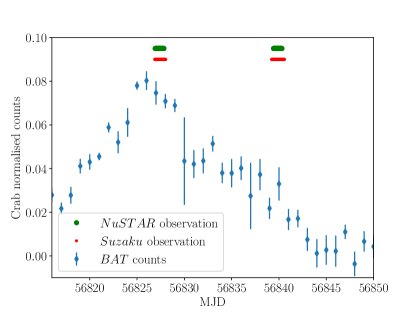
Figure 1: Swift-BAT lightcurve of the 2014 outburst of Cep X-4 (blue circles). The horizontal green and red lines near the top indicate periods of NuSTAR and Suzaku observations respectively. In this work, we refer to the pair of observations near the peak of the outburst as Obs 1, and to observations during the decline of the outburst ($\sim$MJD 56840) as Obs 2.

2.1 NuSTAR data reduction

NuSTAR data were reduced using the standard FTOOL nupipeline software version 1.7.1 (HEAsoft version 6.22) and NuSTAR CALDB version 20171002. Total exposure time after screening the data for Obs 1 was $\sim$40 ks and for Obs 2 was $\sim$41 ks. Source counts were extracted from a circular region of 120″ radius centred on the source coordinates, while background counts were extracted from a circular region of 90″ radius farthest away from the source. We applied barycentric correction with FTOOL barycorr and extracted pulse phase resolved spectra using FTOOL xselect.

2.2 Suzaku data reduction

Suzaku data were reprocessed and screened applying standard criteria using aepipeline (HEAsoft version 6.16). We used CALDB version 20150105 for XIS and version 20110913 for HXD. We performed attitude correction using FTOOL aeattcor2. The data were corrected to the solar system barycenter. We extracted the XIS lightcurves and spectra using the FTOOL xselect and HXD/PIN lightcurves and spectra using the Suzaku specific FTOOLS hxdpinxbpi and hxdpinxblc respectively.

Only XIS3 data could be used for the data analysis as XIS1 had a mode switch during Obs 1 and XIS0 had incomplete and strongly misaligned image with low count rates, while XIS0 and XIS1 were terminated during Obs 2. XIS3 was operated in 1/4 window mode during Obs 1. Source photons were extracted from an annulus with an outer radius 100″ for both observations. To avoid pileup effects of over 4%, we excluded the central 45″ and 10″  regions in Obs 1 and Obs 2 respectively. For both of the observations we combined the data from $3\times 3$ and $5\times 5$ editing modes. The background counts were extracted from a circular region of radius 100″ in the outer regions of the chip and sufficiently far away from the source.

3 Spectral analysis

We first undertake phase-averaged analysis for both Obs 1 and Obs 2 in §3.1, to compare our NuSTAR+Suzaku results with our older NuSTAR+Swift results (FF15). Next, in §3.2, we divide the data into nine phase bins and examine the variations of model parameters with pulse phase. Finally, we synthesise phase-averaged spectra from phase-resolved model spectra, and examine them for the asymmetric line profile in §3.3.

3.1 Phase averaged analysis

We adopt the continuum model used by FF15  and McBride et al. (2007): an absorbed soft black-body and a harder power law (PL) spectrum with a Fermi-Dirac cut-off (FDCUT) (Tanaka, 1986) of the form:

$$F(E)\propto E^{-\Gamma}\left(\frac{1}{1+e^{-(E-E_{\rm{cut}})/E_{\rm{fold}}}}\right)$$ (1)

Absorption by neutral hydrogen was included using the XSPEC phabs model with the abundances from Wilms et al. (2000) and using the cross sections from Verner et al. (1996). To improve the fit an absorption line was added at 30 keV. This line, detected by various authors (see, e.g., McBride et al., 2007), is expected to be a CRSF. In concordance with FF15, we find evidence of a secondary absorption feature at 18 keV. The strength of this feature is lower than the 30 keV line, leading to our interpretation of this being an asymmetric feature of the primary 30 keV cyclotron line. We do not find any evidence for a second harmonic at higher energies. The quality of fits improves further when we include the Fe K$\alpha$ line as a Gaussian feature at $\sim 6.4$ keV. With this final model, phabs*gabs*gabs*(bbodyrad+gaussian+fdcut*powerlaw) (Model 1), we get satisfactory fits with $\chi^{2}=4708$ with 4199 degrees of freedom in Obs 1, and $\chi^{2}=4073$ with 3794 degrees of freedom in Obs 2. Our parameter values from this NuSTAR and Suzaku data set confirm the findings of FF15 from NuSTAR and Swift-XRT data (Table 3).

Jaisawal & Naik (2015) and Vybornov et al. (2017) reported the detection of a harmonic to the CRSF. The ratio of the harmonic energy to CRSF energy is found to be $\sim 1.8$ which is lower than the expected value of 2. The data in the energy range above 50 keV are dominated by the background for both NuSTAR and Suzaku. Thus the parameters of the harmonic line can be expected to depend on the uncertainty level of the background. The cyclotron line and the harmonic are well localised and excluding the harmonic does not affect the continuum (Vybornov et al., 2017). Since the focus of the current work is to study the fundamental CRSF, we restrict the studied energy range to $<50$ keV for NuSTAR and $<45$ keV for Suzaku XIS.

3.2 Pulse phase resolved analysis

We used efsearch to measure a pulse period of 66.335${}^{+0.003}_{-0.004}$ s and 66.333${}^{+0.007}_{-0.011}$ s in Obs 1 and Obs 2 respectively. We then selected a sharp feature in intensity, visible in both observations, as phase 0. This corresponds to barycentric MJD 56826.000023 for Obs 1 and MJD 56839.000215 for Obs 2. The energy resolved pulse profiles of the source are shown in Figure 3. For both observations, the pulse profile varies with energy. Several features get smoothed over at higher energies. In particular, the sharp feature used to define phase 0 is not seen above 10 keV. We also note that the pulse fraction seems to slightly increase with energy up to the 20–40 keV band (seen from the variation in the root-mean-squared values of the pulsed profile), beyond which the data are very noisy and the pulse cannot be detected significantly. To investigate this energy dependence quantitatively, we undertook pulse phase-resolved spectroscopy.

We divided the pulse profile into 9 bins (a–i), as shown in Figure 2. The phases of the boundaries are given in Table 4. The phase boundaries were chosen at distinct transition points which include sharp changes in the local slope of the profile. Although Obs 1 and Obs 2 were analysed separately, the same phase boundaries were used for both. As background is not expected to vary significantly over pulse phase, for fitting each observation we used the respective phase-averaged background spectra. The spectra from all the instruments were rebinned to a minimum of 20 counts per bin for fitting purposes.

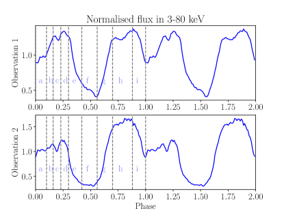
Figure 2: Variation of 3–80 keV flux with pulse phase, as observed by NuSTAR. Two cycles are shown for clarity. The top panel shows the the lightcurve for Obs 1, folded on the pulse period of 66.335 s and divided into 100 uniformly spaced bins for plotting. Similarly, the bottom panel shows the lightcurve for Obs 2 folded on the corresponding period of 66.333 s. Vertical dashed lines shown in the first cycle, indicate the boundaries for the phase-resolved spectroscopy (Table 4).

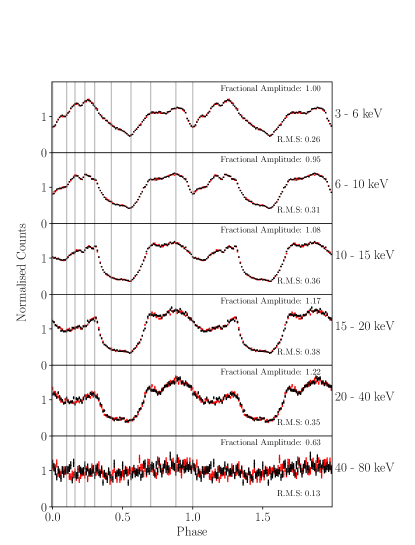
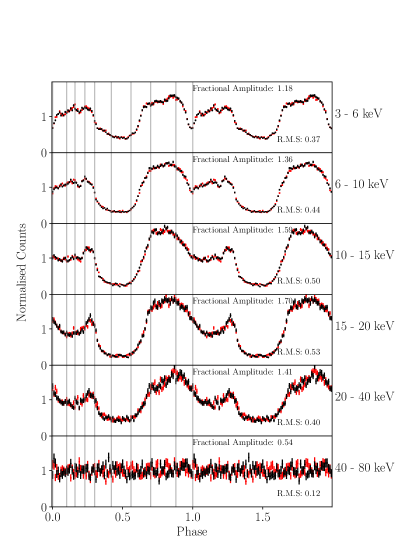
Figure 3: Energy resolved pulse profiles of Obs 1 (Left panel) and Obs 2 (Right panel). The points in red correspond to NuSTAR FPMA counts, while the points in black correspond to NuSTAR FPMB counts, both normalised to the mean count rate in the respective energy bin. The y-axis for each box spans ranges from 0–2 in normalised units. Inset numbers show the root-mean-squared variability and the fractional amplitude across phase for each energy band. Vertical grey lines correspond to the phase boundaries used in the analysis in § 3.2. The labelling of the phases is shown in Figure 2, with boundaries defined in Table 4.

The spectra for individual phases have been plotted in Figure 4, (See left panel for Obs 1 and right for Obs 2). The consecutive spectra are scaled by a constant factor (40) to demonstrate the shape of the spectra. The spectrum for phase ‘a’ (bottom spectrum in each panel) is unscaled. We fit each of these spectra with the spectral model phabs*gabs*(bbodyrad+gaussian+fdcut*powerlaw) (Model 2). The cross normalisations for the instruments were frozen to the phase averaged values. The quality of data in individual phases was not good enough to constrain the iron line parameters, hence these were kept frozen to the values obtained in phase-averaged spectroscopy (§3.1). The freezing of iron line parameters led to increase of $\chi^{2}$ by up to $\sim$10 for all the phases, but we consider it acceptable as the “best-fit” line parameters obtained for individual phases are highly unphysical.

As attempted in §3.1 (and by FF15), another gaussian absorption line was added at 18 keV in the model for the phase bins, but it improved the $\chi^{2}$ by only small amounts ($<10$) for three additional parameters. This is also visually evident in the Figure 5, where the ratio of the data to model is shown for each of the phase bin. For clarity, the consecutive ratio plots are offset by a constant amount (1) and the ratio plot for phase ‘a’ is kept at the actual value. An unmodelled absorption feature in the residuals, if present, would show up as a dip around the peak of the absorption feature, which is not seen in Figure 5. The significance of the additional gaussian absorption line was tested using Bayesian Information Criterion (BIC, Schwarz, 1978) since the ftest included in XSPEC cannot be used for nested multiplicative models (Orlandini et al., 2012). A model with lower BIC is preferred as a better approximation of the true model. The evidence against a model with higher BIC can be estimated by the difference in BIC for the two models (Kass & Raftery, 1995). BIC was computed for the phases with highest reduction in $\chi^{2}$ from the single line model (Model 2) to the double-lined model (Model 1) (Obs 1: Phase a,d; Obs 2: Phase e,h). In all cases BIC is lower for Model 2 (single line). $\Delta$BIC ($\sim 10$ for the tested phases) rules out the model with higher BIC strongly. Hence we use Model 2 to describe the data from now on.

The variation of the free parameters is tabulated in Table 4 and depicted in Figure 6. We see clear variations in model parameters with pulse phase, which can be understood as a effect of variation of magnetic field strength and other parameters along the different lines of sight probed for different phases. In Obs 1, the variation of $E_{\mathrm{CRSF}}$ with the pulse phase follows the trend of the pulse profile. The Pearson R correlation coefficient for the line parameters with the corresponding value of the pulse profile are tabulated in Table 2. Cyclotron line parameters clearly vary with phase in both observations. The variation of cyclotron line central energy ($E_{\mathrm{CRSF}}$), width ($\sigma_{\mathrm{CRSF}}$), and depth ($d_{\mathrm{CRSF}}$) seems to be correlated with total flux in Obs 1. However, no such correlation is seen in Obs 2 in the declining phase of the outburst. Excluding the data from phase ‘e’ and ‘f’ for Obs 2 leads to a better correlation between the intensity at the pulse phase and cyclotron line parameters.

The temperature of the blackbody for phase ‘a’ seems to be smaller than the rest of the phase bins and the phase-averaged value. The area of the emitting region (derived from $A_{\rm{BB}}$) is also larger than in the other phase bins. To measure the effect of the temperature on the line parameters, we refit the phase bin spectrum while holding the temperature fixed at the phase-averaged value. The normalization of the component was left free. The line parameters thus obtained are consistent with the values reported in Table 4 and the normalization converges to the values suggested by the nearby phase bins.

Table 2: The Pearson R correlation coefficient of the line parameters with the normalised pulse profile intensity for different phases. For Obs 2 the value in parentheses indicate the coefficient computed excluding the phases ‘e’ and ‘f’.

	Obs 1	Obs 2
$E_{\rm CRSF}$	0.557	0.147 (0.783)
$\sigma_{\rm CRSF}$	0.322	0.026 (0.119)
$d_{\rm CRSF}$	0.408	0.230 (0.346)

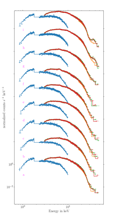
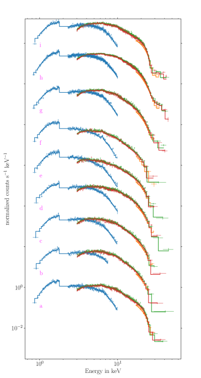
Figure 4: Spectrum for all the phases of Obs 1 (Left panel) and Obs 2 (Right panel). Spectrum for phase a has been kept at the true value and the rest of the spectra are plotted with a constant offset (multiplied by 40). The blue circle, orange diamond, green triangle and red inverted triangle markers correspond to Suzaku–XIS, Suzaku–HXD, NuSTAR–FPMA and NuSTAR–FPMB spectra respectively. For plotting purposes only, the spectra were rebinned to have a significance of $10\sigma$ per bin, to clearly show the shape of the spectrum.

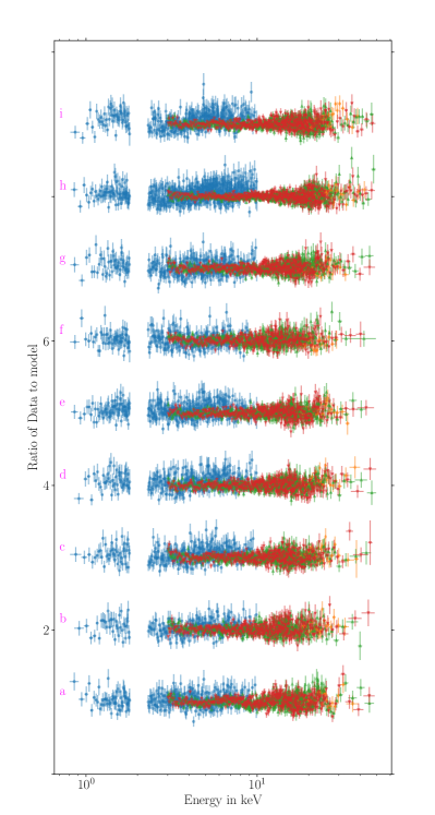
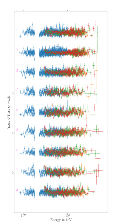
Figure 5: Residuals in form of ratio of data to model for all the phases of Obs 1 (Left panel) and Obs 2 (Right panel). Residuals for phase a has been kept at the true value and the rest of the spectra are plotted with a constant offset (1). The colour scheme and the rebinning is same as Figure 4. The 18 keV feature seems non existent in the residuals but is clearly seen in the phase averaged case (FF15).

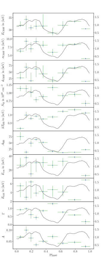
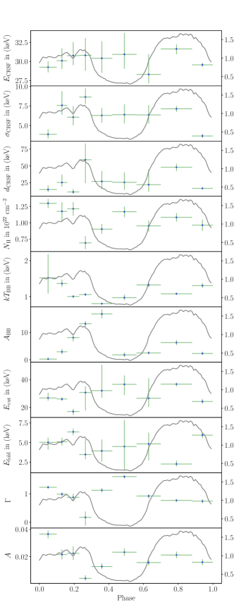
Figure 6: Variation of parameters across pulse phase for Obs 1 and Obs 2. The left panels show the result for Obs 1 and the right panels for Obs 2. The pulse profile in 3-80 keV range for respective observation is shown as a gray line. The most notable feature is that the variation in the cyclotron energy with phase for Obs 1 matches the pulse profile. In Obs 2 except for phases ‘e’ and ‘f’, the line energy follows the trend of the pulse profile as well. $N_{\rm{H}}$ and $\Gamma$ show correlated variability, which may be affected by intrinsic model degeneracy (see Figure 7). The unit for $A_{\rm{BB}}$ is km${}^{2}/(10~{}\rm{kpc})^{2}$ and for A is photons cm^-2 s^-1 keV^-1 at 1 keV.

We also find a dip in the absorbing column density ($N_{\mathrm{H}}$) at the peak in the pulse profile at phase 0.25, followed by a rise in $N_{\mathrm{H}}$ at the intensity dip at phase 0.5. This feature does not fully explain the energy-resolved lightcurves, which show large intensity variations even at high energies. We also note that the power-law index $\Gamma$ and normalisation $A$ show the same phase-resolved trend as $N_{\mathrm{H}}$. A correlated variation in the absorbing column and power-law parameters is often seen in fits. We explore this further by calculating $\chi^{2}$ contours for best-fit models obtained at different values of $N_{\mathrm{H}}$ and $\Gamma$ for each phase (see Figure 7). The plot clearly shows the degeneracy in these two parameters for the fits at each phase. However, we also note that the total range of variations in $\Gamma$ and $N_{\mathrm{H}}$ is higher than the spread seen in individual phases and can therefore be interpreted as a real change in the source parameters.

Different continuum models have an effect on the line parameters. Müller et al. (2013) showed that modelling the continuum shape using a Cutoff power-law (CPL) can result in sharper CRSF features compared to FDCUT+PL. To test whether the wide CRSF parameters were an artifact of the continuum model used here, we also applied the CPL and Negative and Positive power-law with Exponential cutoff (NPEX, Makishima et al., 1999) to the phase resolved data. We find that the line parameters obtained in different continuum models are consistent with each other. Changing continuum model did also not warrant inclusion of the second absorption line in the spectral modelling. The reduction in $\chi^{2}$ is similar to the values obtained with FDCUT+PL.

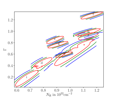
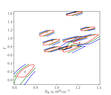
Figure 7: The variation of $N_{\rm{H}}$ with $\Gamma$. The left panel shows the contour plot for Obs 1 while the right panel shows the contour plot for Obs 2. Each set of contours shows the degeneracy between these parameters for various pulse phases, indicated by a letter at the minimum $\chi^{2}$. Red, green and blue contours correspond to $\Delta\chi^{2}$ of 2.3, 4.6 and 9.2 respectively. The degeneracy in the best-fit values for $N_{\rm{H}}$ and $\Gamma$ is evident. However, the full range of variations across all phase bins exceeds the degenerate values of individual bins, and can therefore be interpreted as a real change in the source parameters.

3.3 Adding the models

The clear variation of cyclotron line parameters with phase (Figure 6) leads us to the question if the asymmetric line profile of the phase-averaged spectrum could simply arise by attempting to fit a single model to the phase-averaged spectrum. To test this hypothesis, we took our best-fit models for each phase (§3.2), weighted them by the exposure of each phase bin, and added them together to create a single model. We then simulated a spectrum from this “combined” model using the XSPEC fakeit command. The simulated spectrum was fit with the complete two-component model used by FF15 and in our phase-averaged analysis (§3.1). We find that the spectral parameters obtained for this combined model spectrum are fully consistent with those obtained from the phase-averaged data (Table 3, “Combined model” columns). This striking agreement in the best-fit values indicates that the variation of cyclotron line parameters with phase is a sufficient explanation for the asymmetry in the phase-averaged line profile in Cep X-4. For Obs 1, the combined model when applied to the phase-averaged data without re-fitting results in a $\chi^{2}$ of 4956.05 with 4199 degrees of freedom. The phase averaged spectrum and the combined model have been shown in Figure 8.

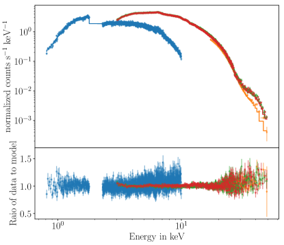
Figure 8: The observed phase averaged spectrum for Obs 1, plotted using the same colour scheme as Figure 4. We compare this data with the “combined model” from §3.3 without any refitting, and obtain a $\chi^{2}$ value of 4956.05 with 4199 degrees of freedom. This combined model is over-plotted on data in the top panel, while the bottom panel shows the ratio of the data to this model (without refitting). Slight excess of the residuals can be seen in XIS from 7-10 keV which can be explained from the slight differences in the parameters between the respective best fits to the phase averaged data and the simulated spectrum from the addition of the models (Table 3).

In this synthesized “combined model” spectrum, the cyclotron line is clearly asymmetric (Figure 9). Notably the fitted parameters in the combined model spectrum are close to the values reported in FF15.

This strongly suggests that the inherent asymmetry detected in the phase-averaged data is explained by the variation of spectral parameters with phase. We note that both single and double-line spectral models give much lower $\chi^{2}$ values when fit to our synthetic data derives from the combined model as compared to the actual phase-averaged data, so there may be small systematic effects in our combining procedure. The improvement obtained by switching from the single-line to double-line model for phase averaged data is much higher ($\Delta\chi^{2}\sim 200$) than for the synthesised data ($\Delta\chi^{2}\sim 40$), which could be attributed to two causes. First, it is possible that there is some inherent asymmetry in the line, which we cannot detect at high significance in the individual phase bins, but asserts itself in the phase-averaged data. The second possibility is that this smaller improvement is simply a result of the $\chi^{2}$ values for fits to synthesised data being already much lower than those for actual phase-averaged data. This interpretation is compatible with the excellent agreement in model parameters for synthesised and observed data. The current dataset will be unable to conclusively establish either of these cases.

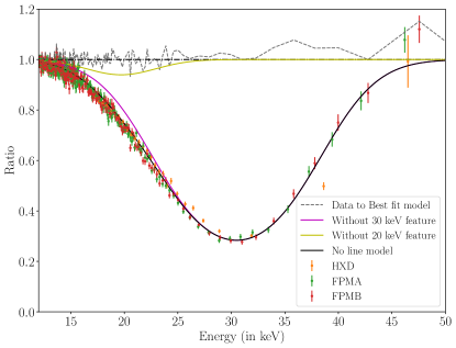
Figure 9: We create a synthetic spectrum from our “combined model” (§3.3) for Obs 1, and fit it with the complete two-line model used in the phase-averaged analysis (§3.1). The dashed gray line shows the ratio of synthetic data to the best-fit two-line model. The flatness of the line shows that the model is a good fit to synthesized data. Next, we set the depths of the two line components to zero, and plot ratios of data to this continuum-only model (without refitting). These data points follow the same colour scheme as Figure 4. A solid black line shows the ratio of this continuum-only model to the complete two-line model. Similarly, the yellow, and magenta lines correspond to models without the 20 keV feature and 30 keV features respectively.

4 Discussion

We analysed NuSTAR and Suzaku data of Cep X-4 obtained during the peak and decline of the 2014 outburst. The spectra are well fit by a model comprised of absorption, a blackbody component, a hard component, an iron line, and a cyclotron feature. We find that this data set gives identical results to those obtained from NuSTAR and Swift-XRT data (FF15). Jaisawal & Naik (2015) and Vybornov et al. (2017) have reported a slightly anharmonic feature of the CRSF. Due to the spectrum being background dominated in this regime, we have excluded NuSTAR data beyond 50 keV and Suzaku XIS data beyond 45 keV in our analysis.

We detect strong pulsations with an $\approx 66.33$ s period in both observations. The pulse profile varies with energy, and in general is smoother at high energies. The pulse fraction slightly increases with the energy as can be seen from the increase in both fractional amplitude and r.m.s. (see Figure 3).

We undertake phase-resolved spectroscopy for both epochs. Data for individual phases are well-fit by a single cyclotron line, with no evidence for an asymmetric line profile like the one seen in phase-averaged spectra. We find clear evidence for variation of spectral parameters with phase. In particular, the cyclotron line energy and width show strong variations. These parameters are correlated with pulse intensity in Obs 1 (at the peak of the outburst), but no obvious correlations are not seen in Obs 2 (outburst decline phase).

We simulate a phase-averaged spectrum by using the weighted sum of the spectral models for each phase. On attempting to fit this “combined model”-based spectrum with our asymmetric line spectral model, we get an excellent fit. The derived parameters are fully consistent with those obtained by fitting the same model to the actual phase-averaged data. Modelling by Schwarm et al. (2017b) indicates that the variation in the parameters can be expected even if the emitting column is uniform. The fit by Schwarm et al. (2017b) to the asymmetric profile of Cep X-4 indicate that the asymmetry can also be explained by assuming a slight anharmonic spacing of the Landau levels coupled with the boosting of the photons due to relativistic electrons. In comparison to this, our work provides the evidence that the asymmetric profile can be obtained after averaging the variation of the parameters seen in different lines of sight. The variation of the physical conditions on the NS surface can also lead to variation in the spectral parameters across the phase bins (Mukherjee & Bhattacharya, 2012).

While an asymmetric line provides a better fit to the combined model, the change in the $\chi^{2}$ value is much smaller than the one obtained for actual phase-averaged data. This effect can arise either due to the line having small, undetectable asymmetry in individual phase bins, or due the generally lower $\chi^{2}$ values obtained for synthesised data. Our current datasets are inadequate to rule out either hypothesis.

Such non-gaussian shapes for CRSFs are predicted by several models (Mukherjee & Bhattacharya, 2012; Schwarm et al., 2017a, b, and references therein), and NuSTAR has the necessary sensitivity and energy resolution for obtaining data to test these models. However, comparison between models and data warrants good measurements of the line parameters and the underlying continuum. Our work shows that the cyclotron features and the continuum component are both strongly dependent on pulse phase in Cep X-4, and any attempts to fit models to data should properly account for these variations. Cep X-4 is a promising start in this direction.

Table 3: Comparing our phase averaged fit to NuSTAR and Suzaku data with the NuSTAR and Swift analysis results of FF15. The phase averaged spectrum is described in § 3.1 while the combined model spectrum is described in § 3.3. The parameters are listed for the model adopted by FF15 which is used for fitting both phase-averaged spectrum and the combined model spectrum. The discrepancy in the blackbody norms ($A_{\rm BB}$) arises from our adoption of the bbodyrad model in XSPEC, as opposed to the blackbody function used by FF15. For completeness, we also list the $\chi^{2}$ values obtained for a model with a single absorption line. We caution that the parameter values in the table are for the two-line model, and different values are obtained for the single-line model.

Component	Parameter	Obs 1			Obs 2
		FF15	Current Work		FF15	Current Work
			Phase averaged	Combined model		Phase averaged	Combined model
Interstellar absorption	$N_{\rm{H}}(10^{22}\rm{cm}^{-2})$	$1.05_{-0.12}^{+0.11}$	$1.06_{-0.04}^{+0.03}$	$1.02\pm 0.04$	$1.41\pm 0.25$	$1.09_{-0.03}^{+0.03}$	$0.97\pm 0.04$
	${A_{\rm{cont}}}^{a}$	$0.061_{-0.010}^{+0.008}$	$0.066\pm 0.004$	$0.060\pm 0.004$	$0.021_{-0.005}^{+0.004}$	$0.0218\pm 0.0007$	$0.022\pm 0.001$
Power law with	$\Gamma$	$0.83_{-0.11}^{+0.07}$	$0.88_{-0.04}^{+0.03}$	$0.80_{-0.06}^{+0.05}$	$0.96_{-0.14}^{+0.09}$	$1.00_{-0.03}^{+0.02}$	$0.76_{-0.04}^{+0.03}$
Fermi Dirac cutoff	$E_{\rm{cut}}$(keV)	$24\pm 4$	$26\pm 2$	$22_{-2}^{+3}$	$25\pm 4$	$28\pm 2$	$26_{-2}^{+3}$
	$E_{\rm{fold}}$(keV)	$5.7_{-0.6}^{+0.5}$	$5.3_{-0.5}^{+0.4}$	$5.9_{-0.5}^{+0.3}$	$5.7_{-0.8}^{+0.6}$	$4.9_{-0.6}^{+0.5}$	$4.9_{-0.6}^{+0.5}$
Cyclotron absorption	$E_{\rm{CRSF}}$(keV)	$30.39_{-0.14}^{+0.17}$	$30.52_{-0.14}^{+0.18}$	$30.5_{-0.14}^{+0.22}$	$29.42_{-0.24}^{+0.27}$	$29.5_{-0.2}^{+0.3}$	$29.5_{-0.2}^{+0.3}$
feature 1	$\sigma_{\rm{CRSF}}$(keV)	$5.8\pm 0.4$	$6.1\pm 0.3$	$5.7_{-0.3}^{+0.4}$	$4.9\pm 0.4$	$5.3\pm 0.3$	$6.1\pm 0.4$
	$d_{\rm{CRSF}}$(keV)	$20_{-4}^{+5}$	$24_{-3}^{+4}$	$18_{-2}^{+4}$	$16.6_{-3.0}^{+4.0}$	$21_{-3}^{+4}$	$23_{-4}^{+6}$
Cyclotron absorption	$E_{\rm{abs}}$(keV)	$19.0_{-0.4}^{+0.5}$	$19.0_{-0.3}^{+0.4}$	$19.7_{-0.9}^{+1.4}$	$18.5\pm 0.7$	$18.0_{-0.5}^{+0.6}$	$17.8_{-0.6}^{+0.8}$
feature 2	$\sigma_{\rm{abs}}$(keV)	$2.5\pm 0.4$	$2.6\pm 0.3$	$3.2_{-0.9}^{+1.1}$	$2.1\pm 0.5$	$2.0\pm 0.4$	$2.5_{-0.6}^{+0.7}$
	$d_{\rm{abs}}$(keV)	$0.60_{-0.17}^{+0.24}$	$0.68_{-0.17}^{+0.24}$	$0.5_{-0.3}^{+0.9}$	$0.37_{-0.15}^{+0.21}$	$0.36_{-0.12}^{+0.16}$	$0.4_{-0.2}^{+0.3}$
Iron line emission	$A$(Fe K$\alpha$)a	$\left(1.39_{-0.14}^{+0.16}\right)\times 10^{-3}$	$\left(1.11_{-0.09}^{+0.10}\right)\times 10^{-3}$	$\left(1.10_{-0.07}^{+0.08}\right)\times 10^{-3}$	$\left(2.8_{-0.6}^{+0.8}\right)\times 10^{-4}$	$\left(1.8\pm 0.3\right)\times 10^{-4}$	$\left(1.6\pm 0.4\right)\times 10^{-4}$
	$\sigma$(Fe K$\alpha$)(keV)	$0.42\pm 0.05$	$0.32_{-0.03}^{+0.04}$	$0.29\pm 0.02$	$0.34_{-0.10}^{+0.12}$	$0.19\pm 0.07$	$0.17_{-0.10}^{+0.08}$
	$E$(Fe K$\alpha$)(keV)	$6.47\pm 0.03$	$6.49\pm 0.02$	$6.48\pm 0.02$	$6.39_{-0.07}^{+0.06}$	$6.42\pm 0.03$	$6.43\pm 0.05$
Blackbody	$A_{\rm{BB}}$	$\left(2.22_{-0.29}^{+0.41}\right)\times 10^{-3}$	$19\pm 2^{b}$	$25\pm 3^{b}$	$\left(7.3_{-1.3}^{+1.7}\right)\times 10^{-4}$	$3.8\pm 0.4^{b}$	$3.8_{-0.6}^{+0.7~{}b}$
	$kT_{\rm{BB}}$(keV)	$0.90\pm 0.03$	$0.960\pm 0.017$	$0.92\pm 0.02$	$0.96\pm 0.06$	$1.09\pm 0.02$	$1.04_{-0.04}^{+0.03}$
Detector	$C_{\rm{FPMB}}$	$1.0319\pm 0.0019$	$1.029\pm 0.001$	$1.029\pm 0.001$	$1.023\pm 0.004$	$1.019\pm 0.002$	$1.016\pm 0.002$
normalization	$C_{\rm{XRT/XIS}}$	$0.962\pm 0.019$	$0.891\pm 0.002$	$0.883\pm 0.002$	$0.91\pm 0.05$	$0.900\pm-0.002$	$0.884\pm 0.002$
	$C_{\rm{HXD}}$		$1.246\pm 0.004$	$1.141\pm 0.002$		$1.249\pm 0.004$	$1.187\pm 0.005$
$\chi^{2}$/dof	Two line model	1215.83/1082	4708.28/4199	4045.28/4192	776.35/670	4073.38/3794	3968.90/3926
$\chi_{\rm{red}}^{2}$		1.124	1.121	0.965	1.159	1.073	1.011
$\chi^{2}$/dof	One line model	1324/1085	4903.03/4202	4085.72/4195	802/673	4127.85/3797	4015.21/3929
$\chi_{\rm{red}}^{2}$		1.22	1.166	0.973	1.19	1.087	1.022

Table 4: Spectral parameters from phase-resolved analysis of Cep X-4 fitted with the model phabs*gabs*(bbodyrad+gaussian+fdcut*powerlaw). The variation of these parameters is depicted in Figure 6 and the results are discussed in § 3.2

Phase bin		a	b	c	d	e	f	g	h	i
Start phase		0	0.1	0.16	0.23	0.30	0.42	0.56	0.70	0.88
End phase		0.1	0.16	0.23	0.30	0.42	0.56	0.70	0.88	1
Parameters		Observation 1
Interstellar absorption	$N_{\rm{H}}$ ($10^{22}$ cm-2)	$1.13\pm 0.08$	$1.13\pm 0.11$	$1.01_{-0.14}^{+0.18}$	$0.78\pm 0.08$	$0.88\pm 0.07$	$1.17_{-0.09}^{+0.08}$	$0.91\pm 0.08$	$0.95\pm 0.07$	$0.67\pm 0.09$
Blackbody	${A_{\rm{BB}}}^{a}$	$75_{-15}^{+18}$	$12\pm 5$	$49_{-14}^{+10}$	$63\pm 4$	$52\pm 4$	$15\pm 3$	$10.7_{-1.7}^{+1.8}$	$12.2\pm 1.6$	$23\pm 3$
	$kT_{\rm{BB}}$(keV)	$0.66\pm 0.04$	$0.99\pm 0.08$	$0.91_{-0.03}^{+0.05}$	$0.97\pm 0.02$	$0.90\pm 0.03$	$0.95_{-0.04}^{+0.03}$	$1.08_{-0.04}^{+0.03}$	$1.13\pm 0.03$	$1.05\pm 0.03$
Power law	${A_{\rm{cont}}}^{b}$	$0.069_{-0.008}^{+0.007}$	$0.099_{-0.015}^{+0.016}$	$0.064_{-0.016}^{+0.022}$	$0.034_{-0.007}^{+0.009}$	$0.050\pm 0.007$	$0.071\pm 0.009$	$0.041\pm 0.006$	$0.045\pm 0.005$	$0.027_{-0.006}^{+0.007}$
with Fermi Dirac	$\Gamma$	$0.92_{-0.08}^{+0.06}$	$0.98\pm 0.08$	$0.61_{-0.24}^{+0.30}$	$0.43_{-0.13}^{+0.11}$	$0.85_{-0.07}^{+0.06}$	$1.28_{-0.08}^{+0.06}$	$0.77_{-0.07}^{+0.06}$	$0.59\pm 0.05$	$0.18_{-0.16}^{+0.14}$
cut off	$E_{\rm{cut}}$(keV)	$27_{-4}^{+11}$	$38_{-12}^{+3}$	$14_{-4}^{+17}$	$30_{-13}^{+6}$	$31_{-7}^{+9}$	$29_{-4}^{+7}$	$33_{-7}^{+4}$	$38.6_{-0.9}^{+0.7}$	$12\pm 2$
	$E_{\rm{fold}}$(keV)	$5.5_{-2.6}^{+0.6}$	$2.9_{-0.7}^{+3.6}$	$6.4_{-3.8}^{+0.4}$	$3.9_{-0.8}^{+1.9}$	$4.2_{-1.7}^{+1.5}$	$4.6_{-1.6}^{+0.9}$	$4.1_{-0.9}^{+1.6}$	$2.33_{-0.19}^{+0.22}$	$6.86\pm 0.17$
Cyclotron	$E_{\rm{CRSF}}$(keV)	$31.7_{-0.4}^{+1.7}$	$34_{-4}^{+1.5}$	$30.8_{-0.9}^{+1.1}$	$31.5_{-1.3}^{+2.3}$	$31.5_{-1.1}^{+4.9}$	$28.7_{-1.0}^{+2.1}$	$31.8_{-1.1}^{+1.7}$	$33.4_{-0.5}^{+0.4}$	$30.43\pm 0.17$
Absorption	$\sigma_{\rm{CRSF}}$(keV)	$6.3_{-0.5}^{+0.9}$	$9.2_{-2.8}^{+0.9}$	$6.9_{-1.1}^{+1.9}$	$9.1_{-0.5}^{+1.2}$	$8.0_{-0.5}^{+1.3}$	$5.9_{-0.9}^{+1.0}$	$8.1_{-0.5}^{+0.7}$	$8.4\pm 0.3$	$4.02_{-0.16}^{+0.18}$
line	$d_{\rm{CRSF}}$(keV)	$28_{-6}^{+24}$	$68_{-41}^{+15}$	$16_{-5}^{+31}$	$61_{-31}^{+29}$	$42_{-16}^{+32}$	$15_{-6}^{+16}$	$46_{-16}^{+15}$	$65\pm 4$	$14.4_{-0.8}^{+0.9}$
	$\chi^{2}/$d.o.f.	$2470.23/2372$	$2082.82/2010$	$2349.73/2269$	$2431.45/2373$	$2506.83/2580$	$2125.74/2167$	$2635.04/2538$	$3393.67/3284$	$2854.08/2786$
Parameters		Observation 2
Interstellar absorption	$N_{\rm{H}}$ ($10^{22}$ cm-2)	$1.29\pm 0.07$	$1.17_{-0.15}^{+0.14}$	$1.21\pm 0.10$	$0.69_{-0.09}^{+0.10}$	$0.90_{-0.07}^{+0.08}$	$1.17\pm 0.08$	$0.95_{-0.09}^{+0.08}$	$1.08\pm 0.06$	$0.96\pm 0.08$
Blackbody	${A_{\rm{BB}}}^{a}$	$0.24_{-0.19}^{+0.62}$	$2.9_{-0.8}^{+1.1}$	$8.1_{-1.3}^{+1.5}$	$13.1_{-0.9}^{+1.0}$	$16.7\pm 1.6$	$1.8_{-0.7}^{+0.9}$	$2.5_{-0.4}^{+0.5}$	$6.3\pm 0.9$	$2.3_{-0.5}^{+0.6}$
	$kT_{\rm{BB}}$(keV)	$1.5_{-0.4}^{+0.6}$	$1.36_{-0.09}^{+0.10}$	$1.00\pm 0.04$	$1.06_{-0.03}^{+0.04}$	$0.80\pm 0.02$	$0.97_{-0.07}^{+0.08}$	$1.32_{-0.06}^{+0.05}$	$1.08\pm 0.03$	$1.30_{-0.06}^{+0.07}$
Power law	${A_{\rm{cont}}}^{b}$	$0.036_{-0.003}^{+0.002}$	$0.021_{-0.003}^{+0.004}$	$0.022\pm 0.005$	$0.0041_{-0.0018}^{+0.0022}$	$0.013\pm 0.002$	$0.023\pm 0.003$	$0.015\pm 0.002$	$0.021\pm 0.002$	$0.016\pm 0.002$
with Fermi Dirac	$\Gamma$	$1.23\pm 0.05$	$0.98_{-0.08}^{+0.07}$	$0.87_{-0.15}^{+0.12}$	$0.17_{-0.28}^{+0.21}$	$1.12\pm 0.07$	$1.60_{-0.06}^{+0.05}$	$0.92_{-0.09}^{+0.06}$	$0.76\pm 0.05$	$0.74_{-0.07}^{+0.06}$
cut off	$E_{\rm{cut}}$(keV)	$27_{-2}^{+4}$	$26.0_{-1.3}^{+1.2}$	$17.0_{-2.4}^{+1.9}$	$30_{-13}^{+4}$	$32_{-5}^{+19}$	$36_{-8}^{+6}$	$27_{-6}^{+14}$	$36.7_{-1.6}^{+1.1}$	$24.2_{-1.6}^{+1.8}$
	$E_{\rm{fold}}$(keV)	$5.0_{-0.9}^{+0.6}$	$5.1\pm 0.5$	$6.4\pm 0.4$	$3.5_{-0.6}^{+1.9}$	$3.9\pm 1.4$	$4.5_{-3.0}^{+3.4}$	$4.8_{-2.1}^{+1.4}$	$2.3_{-0.3}^{+0.4}$	$5.9\pm 0.4$
Cyclotron	$E_{\rm{CRSF}}$(keV)	$29.2_{-0.7}^{+0.8}$	$30.1_{-1.1}^{+1.6}$	$30.8_{-1.2}^{+1.8}$	$30.8_{-2.0}^{+2.2}$	$30.4_{-1.9}^{+2.2}$	$30.9_{-1.9}^{+2.8}$	$28.3_{-1.2}^{+2.6}$	$31.6_{-0.7}^{+0.6}$	$29.6\pm 0.3$
Absorption	$\sigma_{\rm{CRSF}}$(keV)	$3.9_{-0.5}^{+0.6}$	$7.5_{-1.2}^{+1.8}$	$6.0_{-1.0}^{+1.4}$	$8.6_{-0.8}^{+1.1}$	$6.3\pm 0.9$	$6.3_{-1.1}^{+1.3}$	$6.3_{-1.1}^{+1.2}$	$7.1\pm 0.4$	$3.6_{-0.2}^{+0.3}$
line	$d_{\rm{CRSF}}$(keV)	$15_{-3}^{+6}$	$25_{-6}^{+11}$	$11_{-3}^{+4}$	$59_{-34}^{+24}$	$27_{-11}^{+15}$	$25_{-11}^{+14}$	$22_{-10}^{+22}$	$48\pm 5$	$16.6_{-1.7}^{+1.9}$
	$\chi^{2}/$d.o.f	$2255.14/2285$	$1736.34/1646$	$1898.66/1962$	$1930.98/2003$	$1934.30/1930$	$1695.34/1646$	$2495.15/2546$	$3166.90/3159$	$2743.86/2716$

References

- Bonnet-Bidaud & Mouchet (1998) Bonnet-Bidaud J. M., Mouchet M., 1998, Astronomy and Astrophysics, 12, 9
- Caballero & Wilms (2012) Caballero I., Wilms J., 2012, Mem. Soc. Astron. Italiana, 83, 230
- Fürst et al. (2015) Fürst F., et al., 2015, ApJ, 806, L24
- Harrison et al. (2013) Harrison F. A., et al., 2013, ApJ, 770, 103
- Heindl et al. (2004) Heindl W. A., Rothschild R. E., Coburn W., Staubert R., Wilms J., Kreykenbohm I., Kretschmar P., 2004, in Kaaret P., Lamb F. K., Swank J. H., eds, American Institute of Physics Conference Series Vol. 714, X-ray Timing 2003: Rossi and Beyond. pp 323–330 (arXiv:astro-ph/0403197), doi:10.1063/1.1781049
- Jaisawal & Naik (2015) Jaisawal G. K., Naik S., 2015, MNRAS, 453, L21
- Jaisawal & Naik (2017) Jaisawal G. K., Naik S., 2017, in Serino M., Shidatsu M., Iwakiri W., Mihara T., eds, 7 years of MAXI: monitoring X-ray Transients, held 5-7 December 2016 at RIKEN.. p. 153 (arXiv:1705.05536)
- Kass & Raftery (1995) Kass R. E., Raftery A. E., 1995, Journal of the American Statistical Association, 90, 773
- Koyama et al. (1991) Koyama K., et al., 1991, ApJ, 366, L19
- Maitra (2017) Maitra C., 2017, Journal of Astrophysics and Astronomy, 38, 50
- Makishima et al. (1990) Makishima K., et al., 1990, PASJ, 42, 295
- Makishima et al. (1999) Makishima K., Mihara T., Nagase F., Tanaka Y., 1999, ApJ, 525, 978
- McBride et al. (2007) McBride V. A., et al., 2007, A&A, 470, 1065
- Mihara et al. (1990) Mihara T., Makishima K., Ohashi T., Sakao T., Tashiro M., 1990, Nature, 346, 250
- Mihara et al. (1991) Mihara T., Makishima K., Kamijo S., Ohashi T., Nagase F., Tanaka Y., Koyama K., 1991, The Astrophysical Journal, 379, L61
- Mukherjee & Bhattacharya (2012) Mukherjee D., Bhattacharya D., 2012, MNRAS, 420, 720
- Mukherjee et al. (2013) Mukherjee D., Bhattacharya D., Mignone A., 2013, MNRAS, 430, 1976
- Müller et al. (2013) Müller S., et al., 2013, A&A, 551, A6
- Nakajima et al. (2014) Nakajima M., et al., 2014, The Astronomer’s Telegram, 6212
- Orlandini et al. (2012) Orlandini M., Frontera F., Masetti N., Sguera V., Sidoli L., 2012, ApJ, 748, 86
- Roche et al. (1997) Roche P., Green L., Hoenig M., 1997, IAU Circ., 6698
- Schwarm et al. (2017a) Schwarm F.-W., et al., 2017a, A&A, 597, A3
- Schwarm et al. (2017b) Schwarm F.-W., et al., 2017b, A&A, 601, A99
- Schwarz (1978) Schwarz G., 1978, Ann. Statist., 6, 461
- Tanaka (1986) Tanaka Y., 1986, in Mihalas D., Winkler K.-H. A., eds, Lecture Notes in Physics, Berlin Springer Verlag Vol. 255, IAU Colloq. 89: Radiation Hydrodynamics in Stars and Compact Objects. p. 198, doi:10.1007/3-540-16764-1˙12
- Ulmer et al. (1973) Ulmer M. P., Baity W. A., Wheaton W. A., Peterson L. E., 1973, ApJ, 184, L117
- Verner et al. (1996) Verner D. A., Ferland G. J., Korista K. T., Yakovlev D. G., 1996, ApJ, 465, 487
- Vybornov et al. (2017) Vybornov V., Klochkov D., Gornostaev M., Postnov K., Sokolova-Lapa E., Staubert R., Pottschmidt K., Santangelo A., 2017, A&A, 601, A126
- Wilms et al. (2000) Wilms J., Allen A., McCray R., 2000, ApJ, 542, 914
- Wilson et al. (1999) Wilson C. A., Finger M. H., Scott D. M., 1999, ApJ, 511, 367