Dual Pairs and Regularization
of Kummer Shapes in Resonances

Abstract.

We present an account of dual pairs and the Kummer shapes for $n:m$ resonances that provides an alternative to Holm and Vizman’s work. The advantages of our point of view are that the associated Poisson structure on $\mathfrak{su}(2)^{*}$ is the standard $(+)$-Lie–Poisson bracket independent of the values of $(n,m)$ as well as that the Kummer shape is regularized to become a sphere without any pinches regardless of the values of $(n,m)$. A similar result holds for $n:-m$ resonance with a paraboloid and $\mathfrak{su}(1,1)^{*}$. The result also has a straightforward generalization to multidimensional resonances as well.

Tomoki Ohsawa^∗

Department of Mathematical Sciences

The University of Texas at Dallas

800 W Campbell Rd

Richardson, TX 75080-3021, USA

(Communicated by the associate editor name)

1. Introduction

1.1. Kummer Shapes and Dual Pairs in Resonances

Hamiltonian systems with resonant symmetry have been studied quite extensively from many different perspectives. Resonant symmetry crops up in many different forms of $\mathbb{S}^{1}$ symmetries. Although it is one of the simplest symmetries geometrically, it is not only rich in examples and applications but also possesses interesting mathematical structures; see, e.g., Holm [Holm(2011), Chapters 4–6], Dullin et al. [Dullin et al.(2004)Dullin, Giacobbe, and Cushman], Haller [Haller(1999), Chapter 4], and references therein.

From the geometric point of view, Churchill et al. [Churchill et al.(1983)Churchill, Kummer, and Rod], Kummer [Kummer(1981), Kummer(1986), Kummer(1987)] made a seminal contribution by introducing what is now often referred to as the Kummer shapes. Recently Holm and Vizman [Holm and Vizman(2012)] discovered a Poisson-geometric structure behind the Kummer shapes by finding a dual pair of Poisson maps (see, e.g., Weinstein [Weinstein(1983)] and Ortega and Ratiu [Ortega and Ratiu(2004), Chapter 11]) in $n:m$ resonances.

1.2. Main Results and Outline

We build on the work of Holm [Holm(2011), Chapter 4] and Holm and Vizman [Holm and Vizman(2012)] to provide an alternative view of the dual pair constructed in [Holm and Vizman(2012)] as well as of the Kummer shapes in $n:m$, $n:-m$, and multidimensional resonances.

Our approach is to relate $n:m$ resonance with any $(n,m)\in\mathbb{N}^{2}$ with the $1:1$ resonance case; this relationship along with the dual pair from [Holm and Vizman(2012)] (see also Golubitsky et al. [Golubitsky et al.(1987)Golubitsky, Stewart, and Marsden]) for $1:1$ resonance naturally gives rise to the dual pair for $n:m$ resonance; see Theorem 2.1. Our dual pair for $n:m$ resonances is slightly different from that of [Holm and Vizman(2012)]. Specifically, the Poisson structure on $\mathfrak{su}(2)^{*}$ in our dual pair is the standard $(+)$-Lie–Poisson structure regardless of the values of $(n,m)\in\mathbb{N}^{2}$. This is in contrast to the Poisson structure in [Holm and Vizman(2012)] that depends on the values of $(n,m)\in\mathbb{N}^{2}$. An advantage of this result is that the reduced dynamics in $\mathfrak{su}(2)^{*}$ becomes a standard Lie–Poisson dynamics.

A byproduct of this construction is that the Kummer shapes—which usually arise as various shapes such as beet, lemon, onion, turnip, etc. depending on the values of $n$ and $m$ [Holm(2011), Section 4.4.2]—are all “regularized” to become a sphere.

Section 2.6 shows that a similar approach works between $n:-m$ resonance and $1:-1$ resonance. In this case, again all the Kummer shapes are regularized to become a paraboloid.

We also show, in Section 3, that the argument for $n:m$ resonances easily generalizes to multi-dimensional resonances.

2. Kummer Shapes and Dual Pairs in $n:m$ Resonances

We first briefly review Hamiltonian dynamics with $n:m$ resonant symmetry following Holm [Holm(2011), Chapter 4] and Holm and Vizman [Holm and Vizman(2012)]. We then find a Poisson map that provides a bridge between $n:m$ resonances and the $1:1$ resonance using a change of variables introduced in [Holm(2011), Section A.5.4]. This Poisson map naturally gives rise to a dual pair of Poisson maps for $n:m$ resonances with the standard $(+)$-Lie–Poisson bracket on $\mathfrak{su}(2)^{*}$ by relating it to the dual pair for $1:1$ resonance from Golubitsky et al. [Golubitsky et al.(1987)Golubitsky, Stewart, and Marsden] and Holm and Vizman [Holm and Vizman(2012)]. This gives an alternative account of the dual pairs in $n:m$ resonances that is slightly different from those in Holm and Vizman [Holm and Vizman(2012)]. In fact, the Kummer shapes [Kummer(1981), Churchill et al.(1983)Churchill, Kummer, and Rod, Kummer(1986), Kummer(1987)] turn out to be spheres regardless of the values of $n$ and $m$. We work out an example to illustrate this result, as well as extend the result to $n:-m$ resonances.

2.1. $n:m$ Resonances

Let $\mathbb{S}^{1}=\left\{e^{{\rm i}\theta}\in\mathbb{C}\ |\ \theta\in[0,2\pi)\right\}$ and $\mathbb{C}_{\times}\mathrel{\mathop{:}}=\mathbb{C}\backslash\{0\}$ be the set of non-zero complex numbers, and set

$$\mathbb{C}_{\times}^{2}=\left\{\mathbf{a}=(a_{1},a_{2})\ |\ a_{1},a_{2}\in\mathbb{C}_{\times}\right\}.$$

We equip the manifold $\mathbb{C}_{\times}^{2}$ with the symplectic form

$$\Omega_{\mathbb{C}_{\times}^{2}}\mathrel{\mathop{:}}=-\frac{{\rm i}}{2}\sum_{j=1}^{2}\mathbf{d}a_{j}\wedge\mathbf{d}\bar{a}_{j}=-\mathbf{d}\Theta_{\mathbb{C}_{\times}^{2}},$$ (1)

where

$$\Theta_{\mathbb{C}_{\times}^{2}}\mathrel{\mathop{:}}=\frac{1}{2}\sum_{j=1}^{2}\operatorname{Im}(\bar{a}_{j}\mathbf{d}a_{j}).$$

The associated Poisson bracket is

$$\left\{F,G\right\}_{\mathbb{C}_{\times}^{2}}\mathrel{\mathop{:}}=2{\rm i}\sum_{j=1}^{2}\!\left(\dfrac{\partial F}{\partial a_{j}}\dfrac{\partial G}{\partial\bar{a}_{j}}-\dfrac{\partial G}{\partial a_{j}}\dfrac{\partial F}{\partial\bar{a}_{j}}\right).$$

Let $n,m\in\mathbb{N}$ be a pair of natural numbers and consider the following $\mathbb{S}^{1}$-action on $\mathbb{C}_{\times}^{2}$:

$$\Psi^{n:m}_{(\cdot)}\colon\mathbb{S}^{1}\times\mathbb{C}_{\times}^{2}\to\mathbb{C}_{\times}^{2};\qquad(e^{{\rm i}\theta},(a_{1},a_{2}))\mapsto(e^{{\rm i}n\theta}a_{1},e^{{\rm i}m\theta}a_{2})=\mathrel{\mathop{:}}\Psi^{n:m}_{\theta}(\mathbf{a}).$$ (2)

The corresponding infinitesimal generator is defined for any $\omega\in T_{1}\mathbb{S}^{1}\cong\mathbb{R}$ as follows:

$$\omega^{n:m}_{\mathbb{C}_{\times}^{2}}(\mathbf{a})=\left.\dfrac{d}{d\varepsilon}\Psi^{n:m}_{\varepsilon\omega}(\mathbf{a})\right|_{\varepsilon=0}={\rm i}\,\omega\!\left(na_{1}\dfrac{\partial}{\partial a_{1}}+ma_{2}\dfrac{\partial}{\partial a_{2}}\right)+\text{c.c.},$$

where “c.c.” stands for the complex conjugate of the preceding terms. This is essentially equivalent to the dynamics of two harmonic oscillators with frequencies $n$ and $m$:

$$\dot{a}_{1}={\rm i}na_{1},\qquad\dot{a}_{2}={\rm i}ma_{2}.$$ (3)

One also sees that this is the Hamiltonian vector field corresponding to the function $(n|a_{1}|^{2}+m|a_{2}|^{2})/2$.

2.2. $n:m$ Resonance vs. $1:1$ Resonance

Consider the map

$$f_{n:m}\colon\mathbb{C}_{\times}^{2}\to\mathbb{C}_{\times}^{2};\qquad(a_{1},a_{2})\mapsto\!\left(\frac{a_{1}^{m}}{\sqrt{m}\,|a_{1}|^{m-1}},\frac{a_{2}^{n}}{\sqrt{n}\,|a_{2}|^{n-1}}\right).$$ (4)

This change or coordinates is briefly mentioned in Holm [Holm(2011), Section A.5.4], and is a slight modification of the change of variables introduced in [Holm(2011), Section 4.4], where $\sqrt{m}$ and $\sqrt{n}$ are $m$ and $n$ respectively instead. Note that the map is not one-to-one and hence is not invertible in general.

Let $\mathbf{b}=(b_{1},b_{2})$ be the coordinates for the second copy of $\mathbb{C}_{\times}^{2}$, and equip $\mathbb{C}_{\times}^{2}=\{(b_{1},b_{2})\}$ with the same symplectic structure $\Omega_{\mathbb{C}_{\times}^{2}}$ defined in (1) above, and hence with the same Poisson bracket as the above, i.e.,

$$\left\{F,G\right\}_{\mathbb{C}_{\times}^{2}}\mathrel{\mathop{:}}=2{\rm i}\sum_{j=1}^{2}\!\left(\dfrac{\partial F}{\partial b_{j}}\dfrac{\partial G}{\partial\bar{b}_{j}}-\dfrac{\partial G}{\partial b_{j}}\dfrac{\partial F}{\partial\bar{b}_{j}}\right).$$ (5)

Then it is straightforward calculations (see the proof of Proposition 3.1 below) to see that $f_{n:m}$ is a Poisson map, i.e.,

$$\left\{F\circ f_{n:m},G\circ f_{n:m}\right\}_{\mathbb{C}_{\times}^{2}}=\left\{F,G\right\}_{\mathbb{C}_{\times}^{2}}\circ f_{n:m}.$$

One also sees that $f_{n:m}$ is a local symplectomorphism with respect to $\Omega_{\mathbb{C}_{\times}^{2}}$ as well, i.e., for any $\mathbf{a}\in\mathbb{C}_{\times}^{2}$, there exists an open neighborhood $U$ of $\mathbf{a}$ in $\mathbb{C}_{\times}^{2}$ such that $f_{n:m}|_{U}\colon U\to f_{n:m}(U)$ is symplectic. In fact, $f_{n:m}$ is a local diffeomorphism because those distinct points $a_{1},\tilde{a}_{1}\in\mathbb{C}_{\times}$ such that $a_{1}^{m}/(\sqrt{m}\,|a_{1}|^{m-1})=\tilde{a}_{1}^{m}/(\sqrt{m}\,|\tilde{a}_{1}|^{m-1})$ are on the same circle (i.e., $|a_{1}|=|\tilde{a}_{1}|$) but are separated by angles $2k\pi/m$ with $k=1,\dots,m-1$; the same goes with the second portion of $f_{n:m}$. The (local) symplecticity follows from similar coordinate calculations as above; again see the proof of Proposition 3.1 below for more details.

Let us also define $R_{n:m}\colon\mathbb{C}_{\times}^{2}\to\mathbb{R}$ by

$$R_{n:m}(\mathbf{a})\mathrel{\mathop{:}}=\frac{1}{2}\!\left(\frac{|a_{1}|^{2}}{m}+\frac{|a_{2}|^{2}}{n}\right).$$

Clearly it satisfies $R_{n:m}=R_{1:1}\circ f_{n:m}$, and $nmR_{n:m}$ is the Hamiltonian function whose corresponding vector field gives (3), i.e., $R_{n:m}$ is essentially the momentum map corresponding to the action (2).

Now consider the following natural action of the special unitary group $\mathsf{SU}(2)$ on $\mathbb{C}_{\times}^{2}$:

$$\Phi_{(\cdot)}\colon\mathsf{SU}(2)\times\mathbb{C}_{\times}^{2}\to\mathbb{C}_{\times}^{2};\qquad(U,\mathbf{b})\mapsto U\mathbf{b}=\mathrel{\mathop{:}}\Phi_{U}(\mathbf{b}).$$ (6)

It is then clear that $R_{1:1}$ is invariant under the action, i.e., $R_{1:1}\circ\Phi_{U}=R_{1:1}$ for any $U\in\mathsf{SU}(2)$. The momentum map $\mathbf{J}_{1:1}\colon\mathbb{C}_{\times}^{2}\to\mathfrak{su}(2)^{*}$ corresponding to the above action is then given by

$$\mathbf{J}_{1:1}(\mathbf{b}) ={\rm i}\!\left(\mathbf{b}\mathbf{b}^{*}-\frac{1}{2}|\mathbf{b}|^{2}I\right)$$

$$={\rm i}\begin{bmatrix}\frac{1}{2}(|b_{1}|^{2}-|b_{2}|^{2})&b_{1}\bar{b}_{2}\vskip 3.0pt plus 1.0pt minus 1.0pt\\ b_{2}\bar{b}_{1}&-\frac{1}{2}(|b_{1}|^{2}-|b_{2}|^{2})\end{bmatrix}$$

$$=\!\left(\operatorname{Re}(b_{1}\bar{b}_{2}),\,\operatorname{Im}(b_{1}\bar{b}_{2}),\,\frac{1}{2}(|b_{1}|^{2}-|b_{2}|^{2})\right).$$ (7)

See Lemma 3.2 below for a generalization of this result and a proof. Note that we also identified $\mathfrak{su}(2)\cong\mathfrak{su}(2)^{*}$ with $\mathbb{R}^{3}$ as follows:

$$\mathfrak{su}(2)^{*}\cong\mathfrak{su}(2)\to\mathbb{R}^{3};\qquad{\rm i}\begin{bmatrix}\xi_{3}&\xi_{1}+{\rm i}\xi_{2}\\ \xi_{1}-{\rm i}\xi_{2}&-\xi_{3}\end{bmatrix}\mapsto\boldsymbol{\xi}=(\xi_{1},\xi_{2},\xi_{3}).$$

Clearly $\mathbf{J}_{1:1}$ is equivariant, i.e., $\mathbf{J}_{1:1}\circ\Phi_{U}=\operatorname{Ad}_{U^{-1}}^{*}\mathbf{J}_{1:1}(\mathbf{b})$ for any $U\in\mathsf{SU}(2)$.

2.3. The Lie–Poisson Bracket

Let $\mathfrak{su}(2)^{*}_{+}$ be $\mathfrak{su}(2)^{*}$ equipped with $(+)$-Lie–Poisson bracket: For any $F,G\in C^{\infty}(\mathfrak{su}(2)^{*})$,

$$\left\{F,G\right\}_{+}(\mu)\mathrel{\mathop{:}}=\left\langle\mu,\left[\dfrac{\partial F}{\partial\mu},\dfrac{\partial G}{\partial\mu}\right]\right\rangle=2\boldsymbol{\mu}\cdot(\nabla F(\boldsymbol{\mu})\times\nabla G(\boldsymbol{\mu})),$$ (8)

where we identified $\mathfrak{su}(2)^{*}$ with $\mathfrak{su}(2)$ via the inner product

$$\left\langle\xi,\eta\right\rangle\mathrel{\mathop{:}}=\frac{1}{2}\mathop{\mathrm{tr}}\nolimits(\xi^{*}\eta)=\boldsymbol{\xi}\cdot\boldsymbol{\eta}$$

on $\mathfrak{su}(2)$ and hence $\mathfrak{su}(2)^{*}$ is identified with $\mathbb{R}^{3}$ using the identification $\mathfrak{su}(2)\cong\mathbb{R}^{3}$ above. Hence

$$\mu=\begin{bmatrix}\mu_{3}&\mu_{1}+{\rm i}\mu_{2}\\ \mu_{1}-{\rm i}\mu_{2}&-\mu_{3}\end{bmatrix}\in\mathfrak{su}(2)^{*},$$

whereas $\boldsymbol{\mu}=(\mu_{1},\mu_{2},\mu_{3})\in\mathbb{R}^{3}$ here. Note that the above Poisson bracket satisfy

$$\left\{\mu_{i},\mu_{j}\right\}_{+}=2\mu_{k}$$

for any even permutation $(i,j,k)$ of $(1,2,3)$.

Since the $\mathsf{SU}(2)$-action $\Phi$ defined in (6) is a left action and the momentum map $\mathbf{J}_{1:1}\colon\mathbb{C}_{\times}^{2}\to\mathfrak{su}(2)^{*}$ is equivariant, $\mathbf{J}_{1:1}$ is a Poisson map (see, e.g., Marsden and Ratiu [Marsden and Ratiu(1999), Theorem 12.4.1]) with respect to the Poisson bracket (5) and (8), i.e., for any $F,G\in C^{\infty}(\mathfrak{su}(2)^{*})$,

$$\left\{F,G\right\}_{+}\circ\mathbf{J}_{1:1}=\left\{F\circ\mathbf{J}_{1:1},G\circ\mathbf{J}_{1:1}\right\}_{\mathbb{C}_{\times}^{2}}.$$

In fact, Holm and Vizman [Holm and Vizman(2012)] (see also [Golubitsky et al.(1987)Golubitsky, Stewart, and Marsden]) showed that $R_{1:1}$ and $\mathbf{J}_{1:1}$ form a dual pair of Poisson maps:

(9)

that is, $(\ker T_{\mathbf{a}}R_{1:1})^{\Omega}=\ker T_{\mathbf{a}}\mathbf{J}_{1:1}$ for any $\mathbf{a}\in\mathbb{C}_{\times}^{2}$.

2.4. $n:m$ Resonance Invariants

Let us combine the map $f_{n:m}$ from (4) and the momentum map $\mathbf{J}_{1:1}$ from (7) to define

$$\mathbf{J}_{n:m}\colon\mathbb{C}_{\times}^{2}\to\mathfrak{su}(2)^{*}\cong\mathbb{R}^{3};\qquad\mathbf{J}_{n:m}\mathrel{\mathop{:}}=\mathbf{J}_{1:1}\circ f_{n:m}.$$

In coordinates, we have

$$\mathbf{J}_{n:m}(\mathbf{a})=\Bigl{(}\operatorname{Re}\!\left(\frac{a_{1}^{m}\bar{a}_{2}^{n}}{\sqrt{nm}|a_{1}|^{m-1}|a_{2}|^{n-1}}\right),\,\operatorname{Im}\!\left(\frac{a_{1}^{m}\bar{a}_{2}^{n}}{\sqrt{nm}|a_{1}|^{m-1}|a_{2}|^{n-1}}\right),\,\\ \frac{1}{2}\!\left(\frac{|a_{1}|^{2}}{m}-\frac{|a_{2}|^{2}}{n}\right)\Bigr{)}.$$

These are essentially the “invariants” (of (3) but not necessarily invariants of a general Hamiltonian system in $n:m$ resonance) from [Holm(2011), Proposition 4.4.1 on p. 266] although the expressions are slightly different.

Note that $\mathbf{J}_{n:m}$ is also slightly different from the corresponding map $\Pi$ in Holm and Vizman [Holm and Vizman(2012)] as well. This difference leads to an alternative construction of a dual map as well as different Kummer shapes as we shall see in the next subsection.

2.5. Dual Pairs and Kummer Shapes

We are now ready to describe our account of dual pairs and Kummer shapes in $n:m$ resonances. Specifically, our result identifies a relationship between the dual pair (9) of the $1:1$ resonance and $n:m$ resonances as well as the momentum map origin of the dual pairs of Poisson maps for $n:m$ resonances.

Theorem 2.1.

The Poisson maps $R_{n:m}\colon\mathbb{C}_{\times}^{2}\to\mathbb{R}$ and $\mathbf{J}_{n:m}\colon\mathbb{C}_{\times}^{2}\to\mathfrak{su}(2)^{*}_{+}$ are a dual pair for any pair of natural numbers $(n,m)\in\mathbb{N}^{2}$, i.e., for any $\mathbf{a}\in\mathbb{C}_{\times}^{2}$, $\ker T_{\mathbf{a}}R_{n:m}$ and $\ker T_{\mathbf{a}}\mathbf{J}_{n:m}$ are symplectic orthogonal complements to each other. Moreover, the dual pair of Poisson maps for $n:m$ resonances is related to the dual pair of momentum maps $R_{1:1}$ and $\mathbf{J}_{1:1}$ as is shown in the diagram below.

Proof.

We know from Holm and Vizman [Holm and Vizman(2012), Theorem 3.1] that the bottom part constitutes a dual pair: For any $\mathbf{b}\in\mathbb{C}_{\times}^{2}$, $\ker T_{\mathbf{b}}R_{1:1}$ and $\ker T_{\mathbf{b}}\mathbf{J}_{1:1}$ are symplectic orthogonal complements to each other with respect to $\Omega_{\mathbb{C}_{\times}^{2}}$, i.e., $(\ker T_{\mathbf{b}}R_{1:1})^{\Omega}=\ker T_{\mathbf{b}}\mathbf{J}_{1:1}$. However, since $R_{n:m}=R_{1:1}\circ f_{n:m}$, we see that, for any $\mathbf{a}\in\mathbb{C}_{\times}^{2}$,

$$T_{\mathbf{a}}R_{n:m}=T_{f_{n:m}(\mathbf{a})}R_{1:1}\circ T_{\mathbf{a}}f_{n:m}.$$

Now recall that $f_{n:m}$ is a local diffeomorphism; so we have

$$\ker T_{\mathbf{a}}R=(T_{\mathbf{a}}f_{n:m})^{-1}(\ker T_{f_{n:m}(\mathbf{a})}R_{1:1}).$$

Similarly,

$$\ker T_{\mathbf{a}}\mathbf{J}_{n:m}=(T_{\mathbf{a}}f_{n:m})^{-1}(\ker T_{f_{n:m}(\mathbf{a})}\mathbf{J}_{1:1})$$

because $\mathbf{J}_{n:m}=\mathbf{J}_{1:1}\circ f_{n:m}$. Since $f_{n:m}$ is a local symplectomorphism with respect to $\Omega_{\mathbb{C}_{\times}^{2}}$, we conclude that $(\ker T_{\mathbf{a}}R_{n:m})^{\Omega}=\ker T_{\mathbf{a}}\mathbf{J}_{n:m}$ for any $\mathbf{a}\in\mathbb{C}_{\times}^{2}$. ∎

Basic results on dual pairs (see Weinstein [Weinstein(1983)] and Ortega and Ratiu [Ortega and Ratiu(2004), Chapter 11]) imply that the image $\mathbf{J}_{n:m}(R_{n:m}^{-1}(r))$ of the level set $R_{n:m}^{-1}(r)$ of $R_{n:m}$ at any $r>0$ under the map $\mathbf{J}_{n:m}$ is a symplectic leaf in the image of $\mathbf{J}_{n:m}$ in $\mathfrak{su}(2)^{*}$. This is what Holm [Holm(2011), Section 4.4] refers to as an orbit manifold or Kummer shape.

What does the Kummer shape look like in this setting? It is well known that $\mathsf{SU}(2)$ is a double cover of $\mathsf{SO}(3)$ and the coadjoint action of $\mathsf{SU}(2)$ in $\mathfrak{su}(2)^{*}\cong\mathbb{R}^{3}$ is written as rotations in $\mathbb{R}^{3}$ by corresponding elements in $\mathsf{SO}(3)$, and hence the coadjoint orbit in $\mathfrak{su}(2)^{*}\cong\mathbb{R}^{3}$ are spheres; these are the symplectic leaves in $\mathfrak{su}(2)^{*}$ or the Kummer shape here. In fact, setting $\mu=\mathbf{J}_{n:m}(\mathbf{a})$, we see that

$$\mu_{1}^{2}+\mu_{2}^{2}+\mu_{3}^{2}=R_{n:m}(\mathbf{a})^{2}.$$

Therefore, for any pair $(n,m)\in\mathbb{N}^{2}$, the Kummer shape $\mathbf{J}_{n:m}(R_{n:m}^{-1}(r))$ is a sphere without the north and south poles (which correspond to those cases with $a_{2}=0$ and $a_{1}=0$ respectively that were removed from the outset). To summarize:

Corollary 2.2 (Regularization of Kummer shape).

The Kummer shape formed in $\mathfrak{su}(2)^{*}$ using the dual pair from Theorem 3.3 is the sphere with radius $R_{n:m}(\mathbf{a})$ centered at the origin with the north and south poles removed for any $(n,m)\in\mathbb{N}^{2}$.

Remark 2.3.

This result is seemingly contradictory to those from [Holm(2011), Section 4.4.2] and [Holm and Vizman(2012)] that the Kummer shapes take all kinds of different pinched spheres such as beet, lemon, onion, turnip, etc. depending on the values of $n$ and $m$. The reason for this apparent contradiction is that our definition of the Poisson map $\mathbf{J}_{n:m}$ is slightly different from theirs, and the map regularizes or un-pinches these various Kummer shapes in their setting to spheres.

As stated above, an advantage of our setting is that the Poisson structure in $\mathfrak{su}(2)^{*}$ is simple and standard—the $(+)$-Lie–Poisson structure on $\mathfrak{su}(2)^{*}$—as well as independent of $n$ and $m$, whereas the Poisson structure from [Holm(2011), Holm and Vizman(2012)] is more complicated and dependent on the values of $n$ and $m$. As a result, a Hamiltonian dynamics in $\mathbb{C}_{\times}^{2}$ with $n:m$ resonant symmetry is reduced to the Lie–Poisson equation

$$\dot{\mu}=\left\{\mu,h\right\}_{+}(\mu)$$

or in the vector form,

$$\dot{\boldsymbol{\mu}}=-2\boldsymbol{\mu}\times\nabla h(\boldsymbol{\mu}).$$ (10)

in $\mathfrak{su}(2)^{*}$, where $h\colon\mathfrak{su}(2)^{*}\to\mathbb{R}$ is the reduced Hamiltonian defined as $h\circ\mathbf{J}_{n:m}=H$. The Kummer shape is an invariant submanifold of the dynamics. More specifically, the Kummer shape as the coadjoint orbit in $\mathfrak{su}(2)^{*}$ and regard the above Lie–Poisson system as a Hamiltonian system with respect to the Kirillov–Kostant–Souriau structure (see, e.g., Kirillov [Kirillov(2004), Chapter 1] and Marsden and Ratiu [Marsden and Ratiu(1999), Chapter 14] and references therein) on $\mathfrak{su}(2)^{*}$.

The disadvantage of our approach is that the expression for the Hamiltonian $h$ tends to get complicated because of the expression for $\mathbf{J}_{n:m}$. So it is a trade-off between the simplicities of the reduced Hamiltonian $h$ and the Poisson bracket in $\mathfrak{su}(2)^{*}$.

Example 2.4 (1:2 resonance).

We consider the dynamics in $\mathbb{C}_{\times}^{2}$ with respect to the symplectic structure (1) and the Hamiltonian

$$H(\mathbf{a})=\operatorname{Re}(a_{1}^{2}\bar{a}_{2}).$$

The Hamiltonian system ${\bf i}_{X_{H}}\Omega_{\mathbb{C}_{\times}^{2}}=\mathbf{d}{H}$ yields

$$\dot{a}_{1}=2{\rm i}\,\bar{a}_{1}a_{2},\qquad\dot{a}_{2}={\rm i}\,a_{1}^{2}.$$

Clearly the Hamiltonian $H$ has the $1:2$ resonant symmetry, i.e., $H\circ\Psi^{1:2}_{\theta}=H$ for any $e^{{\rm i}\theta}\in\mathbb{S}^{1}$ (see (2) for the definition of the action $\Psi$), and thus

$$R_{1:2}(\mathbf{a})=\frac{1}{2}\!\left(\frac{|a_{1}|^{2}}{2}+|a_{2}|^{2}\right)$$

is conserved along the dynamics. On the other hand, the map $\mathbf{J}_{1:2}\colon\mathbb{C}_{\times}^{2}\to\mathfrak{su}(2)^{*}$ takes the form

$$\mathbf{J}_{1:2}(\mathbf{a})=\!\left(\operatorname{Re}\!\left(\frac{a_{1}^{2}\bar{a}_{2}}{\sqrt{2}|a_{1}|}\right),\,\operatorname{Im}\!\left(\frac{a_{1}^{2}\bar{a}_{2}}{\sqrt{2}|a_{1}|}\right),\,\frac{1}{2}\!\left(\frac{|a_{1}|^{2}}{2}-|a_{2}|^{2}\right)\right).$$

Let us define the Hamiltonian $h\colon\mathfrak{su}(2)^{*}\to\mathbb{R}$ by $h\circ\mathbf{J}_{1:2}=H$. This yields

$$h(\mu)=2\mu_{1}\sqrt{\left\|\mu\right\|+\mu_{3}},$$

where $\left\|\mu\right\|=\sqrt{\mu_{1}^{2}+\mu_{2}^{2}+\mu_{3}^{2}}$. Then the Kummer shape is defined by $\left\|\mu\right\|=r$ for the constant $r\mathrel{\mathop{:}}=R_{1:2}(\mathbf{a}_{0})$ defined by the initial condition $\mathbf{a}_{0}\in\mathbb{C}_{\times}^{2}$ for the above dynamics.

Now, Theorem 2.1 implies that setting $\mu=(\mu_{1},\mu_{2},\mu_{3})=\mathbf{J}_{1:2}(\mathbf{a})\in\mathfrak{su}(2)^{*}$ reduces the dynamics to a Lie–Poisson dynamics in $\mathfrak{su}(2)^{*}$—more specifically on the coadjoint orbit or the Kummer shape $\left\|\mu\right\|=c$—with respect to the Lie–Poisson bracket (8) and the above Hamiltonian $h$. In fact, the Lie–Poisson equation (10) yields

$$\dot{\mu}_{1}=-\frac{2\mu_{1}\mu_{2}}{\sqrt{r+\mu_{3}}},\qquad\dot{\mu}_{2}=\frac{2\mu_{1}^{2}-4\mu_{3}(r+\mu_{3})}{\sqrt{r+\mu_{3}}},\qquad\dot{\mu}_{3}=4\mu_{2}\sqrt{r+\mu_{3}}$$ (11)

on the Kummer shape $\left\|\mu\right\|=r$.

The orbit of the above Lie–Poisson dynamics is given by the intersection of the sphere $\left\|\mu\right\|=r$ and the level set of the Hamiltonian $h$; see Fig. 1. On the other hand, the standard Kummer shape in the 1:2 resonance would be a “turnip” [Holm(2011), Section 4.4.2], i.e., one of the poles of the sphere is pinched, and the Poisson bracket in the reduced space $\mathfrak{su}(2)^{*}$ is not the standard Lie–Poisson bracket; see Holm and Vizman [Holm and Vizman(2012)].

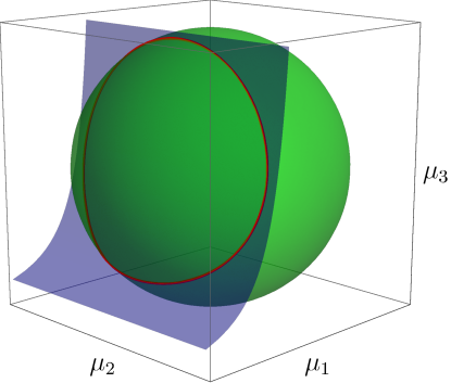
Figure 1. The Kummer shape is regularized to be the sphere (green), and the reduced dynamics (red) (11) is at the intersection of the sphere and the level set (blue) of the Hamiltonian $h$.

2.6. $n:-m$ Resonances

We may easily extend the above construction to those cases where one of the frequencies of resonance is negative. Without loss of generality, let us consider $n:-m$ resonances with $n,m\in\mathbb{N}$. So we consider the action

$$\Psi^{n:-m}_{(\cdot)}\colon\mathbb{S}^{1}\times\mathbb{C}_{\times}^{2}\to\mathbb{C}_{\times}^{2};\qquad(e^{{\rm i}\theta},(a_{1},a_{2}))\mapsto(e^{{\rm i}n\theta}a_{1},e^{-{\rm i}m\theta}a_{2}).$$

on $\mathbb{C}_{\times}^{2}$ equipped with (1). However, equivalently, one may redefine $\bar{a}_{2}$ as $a_{2}$ and instead consider the action $\Psi^{n:m}$ given in (2) on $\mathbb{C}_{\times}^{2}$ equipped with the symplectic form

$$\Omega_{\mathbb{C}_{\times}^{2}}^{1:-1}\mathrel{\mathop{:}}=-\frac{{\rm i}}{2}\sum_{j=1}^{2}k_{j}\mathbf{d}b_{j}\wedge\mathbf{d}\bar{b}_{j}=-\mathbf{d}\Theta_{\mathbb{C}_{\times}^{2}}^{1:-1}$$

with $(k_{1},k_{2})=(1,-1)$, where

$$\Theta_{\mathbb{C}_{\times}^{2}}^{1:-1}\mathrel{\mathop{:}}=\frac{1}{2}\sum_{j=1}^{2}k_{j}\operatorname{Im}(\bar{b}_{j}\mathbf{d}b_{j}).$$

It is a straightforward computation as in $n:m$ resonances to check that $f_{n:m}$ is a local symplectomorphism with respect to $\Omega_{\mathbb{C}_{\times}^{2}}^{1:-1}$ as well as that $f_{n:m}$ is Poisson with respect to the corresponding Poisson bracket: Defining

$$\left\{F,G\right\}_{\mathbb{C}_{\times}^{2}}^{1:-1}\mathrel{\mathop{:}}=2{\rm i}\sum_{j=1}^{2}k_{j}\!\left(\dfrac{\partial F}{\partial b_{j}}\dfrac{\partial G}{\partial\bar{b}_{j}}-\dfrac{\partial G}{\partial b_{j}}\dfrac{\partial F}{\partial\bar{b}_{j}}\right)$$

with $(k_{1},k_{2})=(1,-1)$, we have

$$\left\{F\circ f_{n:m},G\circ f_{n:m}\right\}_{\mathbb{C}_{\times}^{2}}^{1:-1}=\left\{F,G\right\}_{\mathbb{C}_{\times}^{2}}^{1:-1}\circ f_{n:m}.$$

We also define $R_{n:-m}\colon\mathbb{C}_{\times}^{2}\to\mathbb{R}$ as

$$R_{n:-m}(\mathbf{a})\mathrel{\mathop{:}}=\frac{1}{2}\!\left(\frac{|a_{1}|^{2}}{m}-\frac{|a_{2}|^{2}}{n}\right),$$

which satisfies $R_{n:-m}=R_{1:-1}\circ f_{n:m}$.

Let $K\mathrel{\mathop{:}}=\operatorname{diag}(k_{1},k_{2})=\left[\begin{smallmatrix}1&0\\ 0&-1\end{smallmatrix}\right]$ and

$$\mathsf{SU}(1,1) \mathrel{\mathop{:}}=\left\{U\in\mathbb{C}^{2\times 2}\ |\ U^{*}KU=K,\,\det U=1\right\}$$

$$=\left\{\begin{bmatrix}\alpha&\beta\\ \bar{\beta}&\bar{\alpha}\end{bmatrix}\ |\ \alpha,\beta\in\mathbb{C},\,|\alpha|^{2}-|\beta|^{2}=1\right\},$$

and consider the natural action of $\mathsf{SU}(1,1)$ on $(\mathbb{C}_{\times}^{2},\Omega_{\mathbb{C}_{\times}^{2}}^{1:-1})$. Then the corresponding momentum map $\mathbf{J}_{1:-1}\colon\mathbb{C}_{\times}^{2}\to\mathfrak{su}(1,1)^{*}$ is given by

$$\mathbf{J}_{1:-1}(\mathbf{b}) ={\rm i}\!\left(K\mathbf{b}\mathbf{b}^{*}-\frac{1}{2}\mathop{\mathrm{tr}}\nolimits(K\mathbf{b}\mathbf{b}^{*})I\right)$$

$$=\!\left(\operatorname{Re}(b_{1}\bar{b}_{2}),\,-\operatorname{Im}(b_{1}\bar{b}_{2}),\,\frac{1}{2}(|b_{1}|^{2}+|b_{2}|^{2})\right),$$

It is clearly equivariant and thus $\mathbf{J}_{1:-1}$ is a Poisson map with respect to $\Omega_{\mathbb{C}_{\times}^{2}}^{1:-1}$ and the $(+)$-Lie–Poisson bracket on $\mathfrak{su}(1,1)^{*}$. We denote $\mathfrak{su}(1,1)^{*}$ with the $(+)$-Lie–Poisson bracket by $\mathfrak{su}(1,1)^{*}_{+}$ below.

As shown in Holm and Vizman [Holm and Vizman(2012), Theorem 8.1] (see also Iwai [Iwai(1985)]), $R_{1:-1}$ and $\mathbf{J}_{1:-1}$ constitute a dual pair. Hence so do $R_{n:-m}$ and $\mathbf{J}_{n:-m}$ as well, following the same argument as in $n:m$ resonance case. The diagram below summarizes this result.

The Kummer shape in this case is a paraboloid for any $(n,m)\in\mathbb{N}^{2}$. In fact, setting $\mu=\mathbf{J}_{n:-m}(\mathbf{a})$, we have

$$\mu_{3}^{2}-\mu_{1}^{2}-\mu_{2}^{2}=R_{n:-m}(\mathbf{a})^{2}.$$

3. Generalization to Multi-dimensional Resonance

3.1. Setup

Let $\mathbf{a}=(a_{1},\dots,a_{d})$ be coordinates for $\mathbb{C}_{\times}^{d}$, and generalize the symplectic form (1) to $\mathbb{C}_{\times}^{d}$ as follows:

$$\Omega_{\mathbb{C}_{\times}^{d}}\mathrel{\mathop{:}}=-\frac{{\rm i}}{2}\sum_{j=1}^{d}\mathbf{d}a_{j}\wedge\mathbf{d}\bar{a}_{j}=-\mathbf{d}\Theta_{\mathbb{C}_{\times}^{d}},$$ (12)

where

$$\Theta_{\mathbb{C}_{\times}^{d}}\mathrel{\mathop{:}}=\frac{1}{2}\sum_{j=1}^{d}\operatorname{Im}(\bar{a}_{j}\mathbf{d}a_{j}).$$

The associated Poisson bracket is

$$\left\{F,G\right\}_{\mathbb{C}_{\times}^{d}}\mathrel{\mathop{:}}=2{\rm i}\sum_{j=1}^{d}\!\left(\dfrac{\partial F}{\partial a_{j}}\dfrac{\partial G}{\partial\bar{a}_{j}}-\dfrac{\partial G}{\partial a_{j}}\dfrac{\partial F}{\partial\bar{a}_{j}}\right).$$ (13)

We can also generalize the map $f_{n:m}$ introduced in (4) earlier as follows:

Proposition 3.1.

Given a multi-index of natural numbers $\mathbf{n}\mathrel{\mathop{:}}=(n_{1},\dots,n_{d})\in\mathbb{N}^{d}$, let us define $\{\nu_{j}\}_{j\in\{1,\dots,d\}}\subset\mathbb{N}$ by

$$\nu_{j}\mathrel{\mathop{:}}=\prod_{\begin{subarray}{c}1\leq i\leq d\\ i\neq j\end{subarray}}n_{i},$$

and consider the map

$$f_{\mathbf{n}}\colon\mathbb{C}_{\times}^{d}\to\mathbb{C}_{\times}^{d};\qquad\mathbf{a}\mapsto\!\left(\frac{a_{1}^{\nu_{1}}}{\sqrt{\nu_{1}}\,|a_{1}|^{\nu_{1}-1}},\dots,\frac{a_{d}^{\nu_{d}}}{\sqrt{\nu_{d}}\,|a_{d}|^{\nu_{d}-1}}\right).$$

Then $f_{\mathbf{n}}$ is a Poisson map as well as a local symplectomorphism.

Proof.

let $\mathbf{b}=(b_{1},\dots,b_{d})$ be the coordinates for the second copy of $\mathbb{C}_{\times}^{d}$. Then the map $f_{\mathbf{n}}$ is written as $\mathbf{b}=f_{\mathbf{n}}(\mathbf{a})$, and one sees that, for any $j\in\{1,\dots,d\}$,

$$\dfrac{\partial b_{j}}{\partial a_{j}}=\frac{\nu_{j}+1}{2\sqrt{\nu_{j}}}\!\left(\frac{a_{j}}{|a_{j}|}\right)^{\nu_{j}-1},\qquad\dfrac{\partial b_{j}}{\partial\bar{a}_{j}}=-\frac{\nu_{j}-1}{2\sqrt{\nu_{j}}}\!\left(\frac{a_{j}}{|a_{j}|}\right)^{\nu_{j}+1},$$

where the summation on $j$ is not assumed. This implies that, for any $F,G\in C^{\infty}(\mathbb{C}_{\times}^{d})$,

$$\dfrac{\partial(F\circ f_{\mathbf{n}})}{\partial a_{j}}\dfrac{\partial(G\circ f_{\mathbf{n}})}{\partial\bar{a}_{j}}-\dfrac{\partial(G\circ f_{\mathbf{n}})}{\partial a_{j}}\dfrac{\partial(F\circ f_{\mathbf{n}})}{\partial\bar{a}_{j}}=\dfrac{\partial F}{\partial b_{j}}\dfrac{\partial G}{\partial\bar{b}_{j}}-\dfrac{\partial G}{\partial b_{j}}\dfrac{\partial F}{\partial\bar{b}_{j}}$$

as well as

$$\bar{b}_{j}\mathbf{d}b_{j}-b_{j}\mathbf{d}\bar{b}_{j}=\bar{a}_{j}\mathbf{d}a_{j}-a_{j}\mathbf{d}\bar{a}_{j}\iff\operatorname{Im}(\bar{b}_{j}\mathbf{d}b_{j})=\operatorname{Im}(\bar{a}_{j}\mathbf{d}a_{j}).$$

The former equality implies

$$\left\{(F\circ f_{\mathbf{n}}),(G\circ f_{\mathbf{n}})\right\}_{\mathbb{C}_{\times}^{d}}=\left\{F,G\right\}_{\mathbb{C}_{\times}^{d}}\circ f_{\mathbf{n}},$$

and hence $f_{\mathbf{n}}$ is Poisson, whereas the latter implies that $f_{\mathbf{n}}$—which is a local diffeomorphism although it is not globally one-to-one—locally leaves $\Theta_{\mathbb{C}_{\times}^{d}}$ invariant and hence $\Omega_{\mathbb{C}_{\times}^{d}}$ as well. ∎

3.2. Momentum Maps

Let us consider the $\mathbb{S}^{1}$-action

$$\Psi^{\mathbf{n}}_{(\cdot)}\colon\mathbb{S}^{1}\times\mathbb{C}_{\times}^{d}\to\mathbb{C}_{\times}^{d};\qquad(e^{{\rm i}\theta},\mathbf{a})\mapsto(e^{{\rm i}n_{1}\theta}a_{1},\dots,e^{{\rm i}n_{d}\theta}a_{d})=\mathrel{\mathop{:}}\Psi^{\mathbf{n}}_{\theta}(\mathbf{a}).$$ (14)

It is clear that $\Psi^{\mathbf{n}}_{(\cdot)}$ leaves the canonical one-form $\Theta_{\mathbb{C}_{\times}^{d}}$ invariant, i.e., $(\Psi^{\mathbf{n}}_{\theta})^{*}\Theta_{\mathbb{C}_{\times}^{d}}=\Theta_{\mathbb{C}_{\times}^{d}}$ for any $e^{{\rm i}\theta}\in\mathbb{S}^{1}$, and hence is symplectic with respect to $\Omega_{\mathbb{C}_{\times}^{d}}$. The corresponding momentum map is

$$\frac{1}{2}\sum_{j=1}^{d}n_{j}|a_{j}|^{2}=\mathcal{N}\,R_{\mathbf{n}}(\mathbf{a}),$$

where $\mathcal{N}\mathrel{\mathop{:}}=\prod_{j=1}^{d}n_{j}$ and we defined $R_{\mathbf{n}}\colon\mathbb{C}_{\times}^{d}\to\mathbb{R}$ as

$$R_{\mathbf{n}}(\mathbf{a})\mathrel{\mathop{:}}=\frac{1}{2}\sum_{j=1}^{d}\frac{|a_{j}|^{2}}{\nu_{j}}.$$ (15)

Clearly we have $R_{\mathbf{n}}=R_{\mathbf{1}}\circ f_{\mathbf{n}}$.

Let us also consider a natural $\mathsf{SU}(d)$-action on $\mathbb{C}_{\times}^{d}$, i.e.,

$$\Phi_{(\cdot)}\colon\mathsf{SU}(d)\times\mathbb{C}_{\times}^{d}\to\mathbb{C}_{\times}^{d},\qquad(U,\mathbf{b})\mapsto U\mathbf{b}.$$ (16)

and find an expression for the corresponding momentum map for the special case $\mathbf{n}=\mathbf{1}\mathrel{\mathop{:}}=(1,\dots,1)\in\mathbb{N}^{d}$:

Lemma 3.2.

The momentum map $\mathbf{J}_{\mathbf{1}}\colon\mathbb{C}_{\times}^{d}\to\mathfrak{su}(d)^{*}$ corresponding to the above $\mathsf{SU}(d)$-action (16) is given by

$$\mathbf{J}_{\mathbf{1}}(\mathbf{b})={\rm i}\!\left(\mathbf{b}\mathbf{b}^{*}-\frac{1}{d}|\mathbf{b}|^{2}I\right).$$

It is a Poisson map with respect to $\Omega_{\mathbb{C}_{\times}^{d}}$ and the $(+)$-Lie–Poisson bracket on $\mathfrak{su}(d)^{*}$.

Proof.

Let us first find the momentum map $\tilde{\mathbf{J}}\colon\mathbb{C}_{\times}^{d}\to\mathfrak{u}(d)^{*}$ corresponding to the $\mathsf{U}(d)$-action defined the same manner as (16). Let $\xi\in\mathfrak{u}(d)$ be arbitrary. Then the corresponding infinitesimal generator is given by $\xi_{\mathbb{C}_{\times}^{d}}(\mathbf{b})=\xi\mathbf{b}$. Since this action clearly leaves $\Theta_{\mathbb{C}_{\times}^{d}}$ invariant, the momentum map $\tilde{\mathbf{J}}$ is defined by

$$\left\langle\tilde{\mathbf{J}}(\mathbf{b}),\xi\right\rangle=\left\langle\Theta_{\mathbb{C}_{\times}^{d}}(\mathbf{b}),\xi\mathbf{b}\right\rangle,$$

where we define an inner product on $\mathfrak{u}(d)$ as follows:

$$\left\langle\eta,\xi\right\rangle\mathrel{\mathop{:}}=\frac{1}{2}\mathop{\mathrm{tr}}\nolimits(\eta^{*}\xi).$$

We may then identify $\mathfrak{u}(d)^{*}$ with $\mathfrak{u}(d)$ and $\mathfrak{su}(d)^{*}$ with $\mathfrak{su}(d)$ via the above inner product. Now,

$$\left\langle\Theta_{\mathbb{C}_{\times}^{d}}(\mathbf{b}),\xi\mathbf{b}\right\rangle =\frac{1}{2}\operatorname{Im}(\mathbf{b}^{*}\xi\mathbf{b})$$

$$=-\frac{{\rm i}}{2}\mathbf{b}^{*}\xi\mathbf{b}$$

$$=-\frac{{\rm i}}{2}\mathop{\mathrm{tr}}\nolimits(\mathbf{b}\mathbf{b}^{*}\xi)$$

$$=\frac{1}{2}\mathop{\mathrm{tr}}\nolimits\!\left(({\rm i}\mathbf{b}\mathbf{b}^{*})^{*}\xi\right)$$

$$=\left\langle{\rm i}\mathbf{b}\mathbf{b}^{*},\xi\right\rangle,$$

where we used the fact that $\xi^{*}=-\xi$ and hence $\mathbf{b}^{*}\xi\mathbf{b}$ is a pure imaginary number. So we have $\tilde{\mathbf{J}}(\mathbf{b})={\rm i}\,\mathbf{b}\mathbf{b}^{*}$.

Now note that the action $\Phi$ in (16) is the induced subgroup action of of the above $\mathsf{U}(d)$-action. Let $\iota\colon\mathfrak{su}(d)\to\mathfrak{u}(d)$ be the inclusion and $\iota^{*}\colon\mathfrak{u}(d)^{*}\to\mathfrak{su}(d)^{*}$ be its dual. Then the momentum map $\mathbf{J}_{\mathbf{1}}$ is given by $\mathbf{J}_{\mathbf{1}}=\iota^{*}\circ\tilde{\mathbf{J}}$; see, e.g., Marsden and Ratiu [Marsden and Ratiu(1999), Exercise 11.4.2].

By definition, the dual map $\iota^{*}\colon\mathfrak{u}(d)^{*}\to\mathfrak{su}(d)^{*}$ satisfies

$$\left\langle\iota^{*}(\mu),\xi\right\rangle=\left\langle\mu,\iota(\xi)\right\rangle=\left\langle\mu|_{\mathfrak{su}(d)},\xi\right\rangle,$$

and hence $\iota^{*}(\mu)=\mu|_{\mathfrak{su}(d)}$. It is easy to see that the orthogonal complement of $\mathfrak{su}(d)$ in $\mathfrak{u}(d)$ in terms of the above inner product is given by

$$\mathfrak{su}(d)^{\perp}=\operatorname{span}\!\left\{{\rm i}\sqrt{\frac{2}{d}}\,I\right\}.$$

Therefore, using the identification $\mathfrak{u}(d)^{*}\cong\mathfrak{u}(d)$ and $\mathfrak{su}(d)^{*}\cong\mathfrak{su}(d)$, the dual map $\iota^{*}$ is given by the orthogonal projection onto $\mathfrak{su}(d)$:

$$\iota^{*}(\mu) =\mu|_{\mathfrak{su}(d)}$$

$$=\mu-\left\langle{\rm i}\sqrt{\frac{2}{d}}\,I,\mu\right\rangle{\rm i}\sqrt{\frac{2}{d}}\,I$$

$$=\mu-\frac{1}{d}\mathop{\mathrm{tr}}\nolimits(\mu)I.$$

Therefore, we obtain

$$\mathbf{J}_{\mathbf{1}}(\mathbf{b})=\iota^{*}\circ\tilde{\mathbf{J}}(\mathbf{b})={\rm i}\!\left(\mathbf{b}\mathbf{b}^{*}-\frac{1}{d}|\mathbf{b}|^{2}I\right).\qed$$

3.3. Dual Pairs

Now we are ready to generalize Theorem 2.1 to the above multi-dimensional setting. Let $\mathfrak{su}(d)^{*}_{+}$ denote $\mathfrak{su}(d)^{*}$ equipped with the $(+)$-Lie–Poisson bracket on $\mathfrak{su}(d)^{*}$, and define $\mathbf{J}_{\mathbf{n}}\colon\mathbb{C}_{\times}^{d}\to\mathfrak{su}(d)^{*}_{+}$ as $\mathbf{J}_{\mathbf{n}}\mathrel{\mathop{:}}=\mathbf{J}_{\mathbf{1}}\circ f_{\mathbf{n}}$. Then we have the following generalization:

Theorem 3.3.

The Poisson maps $R_{\mathbf{n}}\colon\mathbb{C}_{\times}^{d}\to\mathbb{R}$ and $\mathbf{J}_{\mathbf{n}}\colon\mathbb{C}_{\times}^{d}\to\mathbf{J}_{\mathbf{1}}(\mathbb{C}_{\times}^{d})\subset\mathfrak{su}(d)^{*}_{+}$ are a dual pair for any multi-index $\mathbf{n}\in\mathbb{N}^{d}$ of $d$ natural numbers, i.e., for any $\mathbf{a}\in\mathbb{C}_{\times}^{d}$, $\ker T_{\mathbf{a}}R_{\mathbf{n}}$ and $\ker T_{\mathbf{a}}\mathbf{J}_{\mathbf{n}}$ are symplectic orthogonal complements to each other. Moreover, the dual pair of Poisson maps for the $\mathbf{n}$ resonances is related to the dual pair of momentum maps $R_{\mathbf{1}}$ and $\mathbf{J}_{\mathbf{1}}$ for the $\mathbf{1}$-resonance as is shown in the diagram below.

Proof.

First consider the special case with $\mathbf{n}=\mathbf{1}$. We note in passing that this case is also treated in Cariñena et al. [Cariñena et al.(2014)Cariñena, Ibort, Marmo, and Morandi, Section 5.4.5.3]. It is clear from (15) that $R_{\mathbf{1}}$ is $\mathbb{S}^{1}$ invariant as well as $\mathsf{SU}(d)$ invariant, whereas $\mathbf{J}_{\mathbf{1}}$ is equivariant: From Lemma 3.2, for any $U\in\mathsf{SU}(d)$, we have

$$\mathbf{J}_{\mathbf{1}}(\Phi_{U}(\mathbf{b}))=\operatorname{Ad}_{U^{-1}}^{*}\mathbf{J}_{\mathbf{1}}(\mathbf{b}).$$

Therefore, both $R_{\mathbf{1}}$ and $\mathbf{J}_{\mathbf{1}}$ are Poisson maps; particularly the latter is Poisson with respect to the canonical Poisson bracket (13) on $\mathbb{C}_{\times}^{d}$ and the $(+)$-Lie–Poisson bracket on $\mathfrak{su}(d)^{*}$.

One also sees that $\mathsf{SU}(d)$ acts on the level sets of $R_{\mathbf{1}}$ transitively via the above action $\Phi$ as follows: The level set $R_{\mathbf{1}}^{-1}(r)$ of $R_{\mathbf{1}}$ with any $r>0$ is a $(2d-1)$-dimensional sphere in $\mathbb{C}_{\times}^{d}$ (those points corresponding to the removed origins of the copies of $\mathbb{C}_{\times}$ are removed) centered at the (removed) origin, and thus $\mathsf{SU}(d)$ acts on each level set transitively. It is also clear that every point in $\mathbb{C}_{\times}^{d}$ is a regular point of $R_{\mathbf{1}}$ and $\mathbf{J}_{\mathbf{1}}$; notice that the codomain of $\mathbf{J}_{\mathbf{1}}$ is restricted to the image $\mathbf{J}_{\mathbf{1}}(\mathbb{C}_{\times}^{d})$ in $\mathfrak{su}(d)^{*}_{+}$. Therefore, by Theorem 2.1 of [Holm and Vizman(2012)], $R_{\mathbf{1}}$ and $\mathbf{J}_{\mathbf{1}}$ constitute a dual pair.

The extension to an arbitrary $\mathbf{n}\in\mathbb{N}^{d}$ is a simple generalization of the proof of Theorem 2.1 using Proposition 3.1 as the above diagram shows: Note that we have $R_{\mathbf{n}}=R_{\mathbf{1}}\circ f_{\mathbf{n}}$ and $\mathbf{J}_{\mathbf{n}}=\mathbf{J}_{\mathbf{1}}\circ f_{\mathbf{n}}$ here. ∎

Example 3.4 (1:1:2 resonance).

Let $d=3$ and consider the dynamics in $\mathbb{C}_{\times}^{3}$ with respect to the symplectic structure (12) and the Hamiltonian

$$H(\mathbf{a})=\operatorname{Re}\!\left(a_{1}^{2}(\bar{a}_{2}^{2}+\bar{a}_{3})\right).$$

The Hamiltonian system ${\bf i}_{X_{H}}\Omega_{\mathbb{C}_{\times}^{3}}=\mathbf{d}{H}$ yields

$$\dot{a}_{1}=2{\rm i}\,\bar{a}_{1}(a_{2}^{2}+a_{3}),\qquad\dot{a}_{2}=2{\rm i}\,a_{1}^{2}\bar{a}_{2},\qquad\dot{a}_{3}={\rm i}\,a_{1}^{2}.$$

The Hamiltonian $H$ has $1:1:2$ resonant symmetry, i.e., $H\circ\Psi^{\mathbf{n}}_{\theta}=H$ with $\mathbf{n}=(1,1,2)$ for any $e^{{\rm i}\theta}\in\mathbb{S}^{1}$ (see (14) for the definition of the action $\Psi$), and thus

$$R_{\mathbf{n}}(\mathbf{a})=\frac{1}{4}\!\left(|a_{1}|^{2}+|a_{2}|^{2}+2|a_{3}|^{2}\right)$$

is a conserved quantity for the dynamics.

Let us use a variant $\{\gamma_{j}\}_{j=1}^{8}\subset\mathfrak{su}(3)$ of the Gell-Mann matrices [Gell-Mann(1962)] as a basis for $\mathfrak{su}(3)$ to identify $\mathfrak{su}(3)$ with $\mathbb{R}^{8}$: For any $\xi\in\mathfrak{su}(3)$,

$$\xi=\sum_{j=1}^{8}\xi_{j}\gamma_{j}={\rm i}\begin{bmatrix}\xi_{3}+{\xi_{8}}/{\sqrt{3}}&\xi_{1}+{\rm i}\xi_{2}&\xi_{4}+{\rm i}\xi_{5}\vskip 3.0pt plus 1.0pt minus 1.0pt\\ \xi_{1}-{\rm i}\xi_{2}&{\xi_{8}}/{\sqrt{3}}-\xi_{3}&\xi_{6}+{\rm i}\xi_{7}\vskip 3.0pt plus 1.0pt minus 1.0pt\\ \xi_{4}-{\rm i}\xi_{5}&\xi_{6}-{\rm i}\xi_{7}&-{2\xi_{8}}/{\sqrt{3}}\end{bmatrix}\mapsto\boldsymbol{\xi}=(\xi_{1},\dots,\xi_{8})\in\mathbb{R}^{8}.$$ (17)

We also identify $\mathfrak{su}(3)^{*}$ with $\mathfrak{su}(3)$ as well just as described in the proof of Lemma 3.2.

The map $f_{\mathbf{n}}\colon\mathbb{C}_{\times}^{3}\to\mathbb{C}_{\times}^{3}$ is defined as

$$f_{\mathbf{n}}(\mathbf{a})\mathrel{\mathop{:}}=\!\left(\frac{a_{1}^{2}}{\sqrt{2}\,|a_{1}|},\,\frac{a_{2}^{2}}{\sqrt{2}\,|a_{2}|},\,a_{3}\right),$$

and $\mathbf{J}_{\mathbf{n}}\colon\mathbb{C}_{\times}^{3}\to\mathfrak{su}(3)^{*}$ takes the form

$$\mathbf{J}_{\mathbf{n}}(\mathbf{a})=\Biggl{(}\operatorname{Re}\!\left(\frac{a_{1}^{2}\bar{a}_{2}^{2}}{2|a_{1}||a_{2}|}\right),\,\operatorname{Im}\!\left(\frac{a_{1}^{2}\bar{a}_{2}^{2}}{2|a_{1}||a_{2}|}\right),\,\frac{1}{4}\!\left(|a_{1}|^{2}-|a_{2}|^{2}\right),\,\\ \operatorname{Re}\!\left(\frac{a_{1}^{2}\bar{a}_{3}}{\sqrt{2}|a_{1}|}\right),\,\operatorname{Im}\!\left(\frac{a_{1}^{2}\bar{a}_{3}}{\sqrt{2}|a_{1}|}\right),\,\operatorname{Re}\!\left(\frac{a_{2}^{2}\bar{a}_{3}}{\sqrt{2}|a_{2}|}\right),\,\operatorname{Im}\!\left(\frac{a_{2}^{2}\bar{a}_{3}}{\sqrt{2}|a_{2}|}\right),\,\\ \frac{1}{4\sqrt{3}}\!\left(|a_{1}|^{2}+|a_{2}|^{2}-4|a_{3}|^{2}\right)\Biggr{)}.$$

We define the reduced Hamiltonian

$$h(\mu)\mathrel{\mathop{:}}=4\mu_{1}\sqrt{\mu_{1}^{2}+\mu_{2}^{2}}+2\mu_{4}\!\left(\frac{(\mu_{1}^{2}+\mu_{2}^{2})(\mu_{4}^{2}+\mu_{5}^{2})}{\mu_{6}^{2}+\mu_{7}^{2}}\right)^{1/4}$$

on the open subset

$$\left\{\mu\in\mathfrak{su}(3)^{*}\ |\ (\mu_{1},\mu_{2})\neq 0,\,(\mu_{4},\mu_{5})\neq 0,\,(\mu_{6},\mu_{7})\neq 0\right\}$$

so that it satisfies $h\circ\mathbf{J}_{\mathbf{n}}=H$. The reduced dynamics is then given by the Lie–Poisson equation

$$\dot{\mu}=-\operatorname{ad}_{\partial h/\partial\mu}^{*}\mu.$$

One advantage of our formulation is that one can find the Casimirs relatively easily because the Lie–Poisson bracket is standard. In fact, it is well known that $\mathfrak{su}(3)^{*}$ has quadratic and cubic Casimirs:

$$C_{2}(\mu)\mathrel{\mathop{:}}=\sum_{j=1}^{8}\mu_{j}^{2},\qquad C_{3}(\mu)\mathrel{\mathop{:}}=\sum_{1\leq j,k,l\leq 8}d_{jkl}\mu_{j}\mu_{k}\mu_{l},$$

where the coefficients $\{d_{jkl}\}_{1\leq j,k,l\leq 8}$ are defined so that the basis $\{\gamma_{j}\}_{j=1}^{8}$ for $\mathfrak{su}(3)$ defined in (17) satisfies, for any $j,k\in\{1,\dots,8\}$,

$$\gamma_{j}\gamma_{k}+\gamma_{k}\gamma_{j}=-\frac{4}{3}\delta_{jk}I+2{\rm i}\sum_{l=1}^{8}d_{jkl}\gamma_{l}.$$

This results in the following non-zero coefficients (all the others vanish):

$$d_{118}=d_{228}=d_{338}=-d_{888}=\frac{1}{\sqrt{3}},$$

$$d_{146}=d_{157}=-d_{247}=d_{256}=d_{344}=d_{355}=-d_{366}=-d_{377}=\frac{1}{2},$$

$$d_{448}=d_{558}=d_{668}=d_{778}=-\frac{1}{2\sqrt{3}}.$$

These two Casimirs are conserved along the Lie–Poisson dynamics.

While the geometry of the multi-dimensional generalization of the dual pairs works out nicely, it is not clear if this dual pair is particularly effective in understanding multi-dimensional dynamics in resonance. In fact, in the above example, the resulting Lie–Poisson equation is defined in a higher-dimensional space, $\mathfrak{su}(3)^{*}\cong\mathbb{R}^{8}$, than the original one, $\mathbb{C}_{\times}^{3}$. The extra conserved quantities $C_{2}$ and $C_{3}$ compensate for this increase in dimension, but unfortunately it is not evident whether the Lie–Poisson formulation has a clear advantage over the original formulation.

Received xxxx 20xx; revised xxxx 20xx.

References

• [Cariñena et al.(2014)Cariñena, Ibort, Marmo, and Morandi] J.F. Cariñena, A. Ibort, G. Marmo, and G. Morandi. Geometry from Dynamics, Classical and Quantum. Springer, 2014.
• [Churchill et al.(1983)Churchill, Kummer, and Rod] R. C. Churchill, M. Kummer, and D. L. Rod. On averaging, reduction, and symmetry in Hamiltonian systems. Journal of Differential Equations, 49(3):359–414, 1983.
• [Dullin et al.(2004)Dullin, Giacobbe, and Cushman] H. Dullin, A. Giacobbe, and R. Cushman. Monodromy in the resonant swing spring. Physica D: Nonlinear Phenomena, 190(1):15–37, 2004.
• [Gell-Mann(1962)] M. Gell-Mann. Symmetries of baryons and mesons. Physical Review, 125(3):1067–1084, 1962.
• [Golubitsky et al.(1987)Golubitsky, Stewart, and Marsden] M. Golubitsky, I. Stewart, and J. E. Marsden. Generic bifurcation of Hamiltonian systems with symmetry. Physica D: Nonlinear Phenomena, 24(1–3):391–405, 1987.
• [Haller(1999)] G. Haller. Chaos Near Resonance. Applied Mathematical Sciences. Springer, New York, 1999.
• [Holm(2011)] D. D. Holm. Geometric Mechanics, Part I: Dynamics and Symmetry. Imperial College Press, 2nd edition, 2011.
• [Holm and Vizman(2012)] D. D. Holm and C. Vizman. Dual pairs in resonances. Journal of Geometric Mechanics, 4(3):297–311, 2012.
• [Iwai(1985)] T. Iwai. On reduction of two degrees of freedom Hamiltonian systems by an $S^{1}$ action, and $SO_{0}(1,2)$ as a dynamical group. Journal of Mathematical Physics, 26(5):885–893, 1985.
• [Kirillov(2004)] A. A. Kirillov. Lectures on the Orbit Method. Graduate Studies in Mathematics. American Mathematical Society, 2004.
• [Kummer(1981)] M. Kummer. On the construction of the reduced phase space of a Hamiltonian system with symmetry. Indiana Univ. Math. J., 30:281–291, 1981.
• [Kummer(1986)] M. Kummer. Lecture 1: On resonant hamiltonian systems with finitely many degrees of freedom., volume 252 of Lecture Notes in Physics, pages 19–31. Springer Berlin/Heidelberg, 1986.
• [Kummer(1987)] M. Kummer. On resonant Hamiltonians with $n$ frequencies, volume 278, pages 63–65. Springer Berlin/Heidelberg, 1987.
• [Marsden and Ratiu(1999)] J. E. Marsden and T. S. Ratiu. Introduction to Mechanics and Symmetry. Springer, 1999.
• [Ortega and Ratiu(2004)] J. P. Ortega and T. S. Ratiu. Momentum Maps and Hamiltonian Reduction, volume 222 of Progress in Mathematics. Birkhäuser, 2004.
• [Weinstein(1983)] A. Weinstein. The local structure of Poisson manifolds. Journal of Differential Geometry, 18:523–557, 1983.