Gravitational wave forms, polarizations, response functions and energy losses of triple systems in Einstein-Aether theory

Abstract

Gravitationally bound hierarchies containing three or more components are very common in our Universe. In this paper we study periodic gravitational wave (GW) form, their polarizations, response function, its Fourier transform, and energy loss rate of a triple system through three different channels of radiation, the scalar, vector and tensor modes, in Einstein-aether theory of gravity. The theory violates locally the Lorentz symmetry, and yet satisfies all the theoretical and observational constraints by properly choosing its four coupling constants $c_{i}$’s. In particular, in the weak-field approximations and with the recently obtained constraints of the theory, we first analyze the energy loss rate of a binary system, and find that the dipole contributions from the scalar and vector modes could be of the order of ${\cal{O}}\left(c_{14}\right){\cal{O}}\left(G_{N}m/d\right)^{2}$, where $c_{14}\;(\equiv c_{1}+c_{4})$ is constrained to $c_{14}\lesssim{\cal{O}}\left(10^{-5}\right)$ by current observations, and $G_{N},\;m$ and $d$ are, respectively, the Newtonian constant, mass and size of the source. On the other hand, the “strong-field” effects for a binary system of neutron stars are about six orders lower than that of GR. So, in this paper we ignore these “strong-field” effects and first develop the general formulas to the lowest post-Newtonian order, by taking the coupling of the aether field with matter into account. Within this approximation, we find that the scalar breather mode and the scalar longitudinal mode are all suppressed by a factor of ${\cal{O}}\left(c_{14}\right)$ with respect to the transverse-traceless modes ($h_{+}$ and $h_{\times}$), while the vectorial modes $(h_{X}$ and $h_{Y}$) are suppressed by a factor of $c_{13}\lesssim{\cal{O}}\left(10^{-15}\right)$. Applying the general formulas to a triple system with periodic orbits, we find that the corresponding GW form, response function, and its Fourier transform depend sensitively on the configuration of the triple system, their orientation with respect to the detectors, and the binding energies of the three compact bodies.

I Introduction

The detection of the gravitational wave from the coalescing of two massive black holes (one with mass $36^{+5}_{-4}\;M_{\bigodot}$ and the other with mass $29^{+4}_{-4}\;M_{\bigodot}$) by the advanced Laser Interferometer Gravitational-Wave Observatory (aLIGO) marked the beginning of the era of the gravitational wave (GW) astronomy GW150914 . Following it, five more GWs were detected GW151226 ; GW170104 ; GW170608 ; GW170814 ; GW170817 , and one candidate was identified LVT151012 . The Advanced Virgo detector (aVirgo) aVIRGO joined the second observation run of aLIGO on August 1, 2017, and jointly detected the last two GWs, GW170814 and GW170817 GW170814 ; GW170817 . Except GW170817, which was produced by the merger of binary neutron stars (BNSs) GW170817 , all the rest were produced during the mergers of binary black holes (BBHs). The detection of GW170817 is important, not only because it confirmed that BNSs are indeed one of the most promising sources of GWs, but also because it was companied by a short-duration gamma-ray burst (SGRB) GRB170817 , which enables a wealth of science unavailable from either messenger alone. In particular, it allows us simultaneously to measure both distance and redshift of the source, with which we can study, for example, cosmology.

With the promise of increasing duration, observational sensitivity and the number of detectors, many more events are expected to be detected. In particular, the Laser Interferometer Space Antenna (LISA) LISA is expected to observe tens of thousands of compact galactic binaries during its nominal four year mission lifetime CR17 . As a matter of fact, because of its high mass, GW150914 would have been visible to LISA for several years prior to their coalescence Sesana16 .

Despite significant investigations, the origins of these binary systems, particularly the heavier BBHs, remain an open question (see, for example, Wang18 and references therein). Not only from the point of view of theoretical simulations but also from the observational estimates, it is found very difficult to have such heavy black holes (BHs). On the one hand, most of BHs obtained from numerical simulations have masses lower than $10M_{\bigodot}$, unless the stellar metallicity is very low Fryer12 . On the other hand, Özel et al examined 16 low-mass X-ray binary systems containing BHs, and found that the masses of BHs hardly exceeded $20M_{\bigodot}$, and that there was a strongly peaked distribution at $7.8\pm 1.2M_{\bigodot}$ Ozel10 . Similar results were obtained by Farr et al Farr11 .

To reconcile the above mentioned problem, one of the mechanisms Wang18 is to consider a series mergers of such binary systems in a dense star cluster SH93 ; Banerjee17 . Assuming that such a merger initially occurred with stellar mass ($\simeq 10M_{\bigodot}$) BHs, due to the presence of many massive stars/BHs in the dense cluster, the merger product could easily combine with a third massive companion to trigger another merger. One of the interesting properties of this scenario is that such formed BHs usually have very high spins, and can be easily identified with future aLIGO/aVirgo detections ASTA14 ; LLY15 ; FHF17 ; GB17 . Recently, Rodriguez et al RACR18 considered realistic models of globular clusters with fully post-Newtonian (PN) stellar dynamics for three- and four-body encounters, and found that nearly half of all binary BH mergers occur inside the cluster, and with about 10 $\%$ of those mergers entering the aLIGO/aVirgo band with eccentricities greater than $0.1$. In particular, in-cluster mergers lead to the birth of a second generation (2G) of BHs with larger masses and high spins. These 2G BHs can reconcile the upper BH mass limit $\left(\lesssim 50M_{\bigodot}\right)$ created by the pair-instability supernovae Woosley16 .

Gravitationally bound hierarchies containing three or more components are very common in our Universe Naoz16 . Roughly speaking, about $13\%$ of low-mass stelar systems contains three or more stars FC17 , and $96\%$ of low-mass binaries with periods shorter than 3 days are part of a larger hierarchy Tok06 . The simplest example is the 3-body system of our Sun, Earth and Moon. In fact, any star in the vicinity of a supermassive BH binary naturally forms a triple system.

Recently, a realistic triple system was observed, named as PRS J0337 + 1715 Ransom14 , which consists of an inner binary and a third companion. The inner binary consists of a pulsar with mass $m_{1}=1.44M_{\bigodot}$ and a white dwarf with mass $m_{2}=0.20M_{\bigodot}$ in a 1.6 day orbit. The outer binary consists of the inner binary and a second dwarf with mass $m_{3}=0.41M_{\bigodot}$ in a 327 day orbit. The two orbits are very circular with its eccentricities $e_{I}\simeq 6.9\times 10^{-4}$ for the inner binary and $e_{O}\simeq 3.5\times 10^{-2}$ for the outer orbit. The two orbital planes are remarkably coplanar with an inclination $\lesssim 0.01^{o}$. A triple system is an ideal place to test the strong equivalence principle Shao16 . Remarkably, after 6-year observations, lately it was found that the accelerations of the pulsar and its nearby white-dwarf companion differ fractionally by no more than $2.6\times 10^{-6}$ Archibald18 , which provides the most severe constraint on the violation of the strong equivalence principle.

In a triple system, the existence of the third companion can undertake the Lidov-Kozai oscillations Lidov61 ; Kozai62 , and cause the orbit of the inner binary to become nearly radial, whereby a rapid merger due to GW emissions can be resulted ST17 ; HN18 . Such a system can emit GWs in the 10 Hz frequency band Wen03 ; MKL17 ; Samsing18 , which are potential sources for the current ground-based detectors, such as aLIGO, aVirgo and KAGRA KAGRA . It can also emit GWs in the frequency bands to be detectable by LISA AS12 , and pulsar timing arrays Kocsis12 . In particular, with such a high detectable event rate, it is expected that LISA will detect many triple or higher multiple systems RCTT18 .

In this paper, we shall study the periodic gravitational wave forms, response functions, and energy losses of triple systems in Einstein-aether theory JM01 . This problem is interesting particularly for the orbits in which two of the bodies pass each other very closely and yet avoid their collisions, so they can produce periodic gravitational waves with intension, which are the natural sources for the future detections of GWs. Certainly, this problem is also very challenging, as even in Newtonian theory, the systems allow chaotic and singular solutions, and only few periodic solutions are known MQ14 ; THZ16 . When one of the 3-bodies is a test mass, it reduces to the restricted 3-body problem, and a collinear solution was found by Euler Euler1767 . In 1772 Lagrange found a second class of periodic orbits for an equilateral triangle configuration Lagrange1772 (A historic review of the subject can be found in MQ14 ).

Gravitational wave forms of 3-body systems in general relativity (GR) were calculated up to the 1PN approximations with the orbits of the 3-bodies are still Newtonian THA09 ; DSH14 . In GR, neither analytical nor numerical solutions of 3-body problem of the full theory have been found, and most of the studies were restricted to PN approximations, see, for example, Refs.ICA07 ; LN08 ; Brum03 ; Naoz16 ; BED17 ; RX18 and references therein. In particular, the 1PN collinear solution was found in YA10 and proved that it is unique in YA11 . The 1PN triangular solution and stability were studied, respectively, in IYA11 ; YA12 and YTA15 ; YT17 . Lately, the existence and uniqueness of the 1PN collinear solution in the scalar-tensor theory were studied in ZCX16 ; CZX17 .

In the framework of Einstein-aether theory, Foster Foster07 and Yagi et al Yagi14 derived the metric and equations of motion to the 1PN order for a N-body system. Recently, Will applied them to study the 3-body problem and obtained the accelerations of a 2-body system in the presence of the third body at the quasi-Newtonian order Will18 . For nearly circular coplanar orbits, he also calculated the “strong-field” Nordtvedt parameter $\hat{\eta}_{N}$. For the PRS J0337 + 1715 system, ignoring the sensitivities of the two white-dwarf companions, Will found that $\hat{\eta}_{N}$ is given by $\hat{\eta}_{N}=s_{1}/(1-s_{1})$, where $s_{1}$ denotes the sensitivity of the pulsar.

In this paper, we shall focus ourselves on periodic GWs in the framework of Einstein-aether theory. The theory breaks locally the Lorentz symmetry by the presence of a globally time-like unit vector field - the aether, and allows three different types of gravitational modes, the scalar, vector and tensor JM04 , and all the modes in principle move at different speeds Jacobson . Recently, it was found OMW18 that the four independent coupling constants of the theory must satisfy the constraints of Eq.(2.17) given below, after several conditions are imposed. In the vacuum, GWs were also studied in JM04 ; GHLP18 , while GW forms and angular momentum loss were studied for binary systems in HYY15 ; SY18 , respectively.

The rest of the paper is organized as follows: in Sec. II we give a brief introduction to the Einstein-aether theory, and in Sec. III we first study the effects of the gravitational radiations from the scalar and vector modes to the energy loss for a binary system to the lowest PN order Foster06 , and find that for a neutron star binary system their contributions to the quadrupole, monopole and dipole are, respectively, the orders of ${\cal{O}}\left(10^{-5}\right),\;{\cal{O}}\left(10^{-5}\right)$ and ${\cal{O}}\left({10^{-2}}\right)$ lower than the quadrupole contributions of GR (in which the scalar and vector modes are absent) [cf. Eq.(III)], while the strong field effects are, respectively, the orders of ${\cal{O}}\left({10^{-6}}\right),\;{\cal{O}}\left({10^{-6}}\right)$ and ${\cal{O}}\left({10^{-7}}\right)$ lower. Additionally, the order for the cross term is of ${\cal{O}}\left({10^{-6}}\right)$ lower [cf. Eq.(III.1)]. Similar conclusions can also be obtained by analyzing the amplitudes of polarization modes of a binary system with non-vanishing sensitivities given in HYY15 . Therefore, to the current (second) generation of GW detectors Schutz18 , we can safely ignore these strong field effects. Then, in Sec. IV we consider the lowest PN approximations by taking the coupling of the aether with matter fields into account. When such couplings are turned off, our formulas reduce to the ones presented in Foster06 , subjected to some corrections of typos. From the general expressions for the polarization modes $h_{N}$ given by Eq.(IV.1), we can see that the scalar breather and the scalar longitudinal modes are always proportional to each other, so only five of the six polarization modes are independent. In addition, the two scalar modes are all suppressed by a factor of ${\cal{O}}\left(c_{14}\right)\lesssim{\cal{O}}\left(10^{-5}\right)$ with respect to the transverse-traceless modes ($h_{+}$ and $h_{\times}$), while the vectorial modes $(h_{X}$ and $h_{Y}$) are suppressed by a factor of ${\cal{O}}\left(c_{13}\right)\lesssim{\cal{O}}\left(10^{-15}\right)$. In Sec. V, we apply these formulas to triple systems and obtain the GW forms, response functions, their Fourier transforms, and energy losses for three representative cases. Our results show that the GW forms sensitively depend on not only the configurations of the 3-body orbits, but also their relative positions to the detectors, sharply in contrast to the 2-body problem Mag08 ; PW14 . Our paper is ended with Sec. VI, in which we present our main conclusions.

II Einstein-Aether Theory

In Einstein-aether ($\ae$-) theory, the fundamental variables of the gravitational sector are JM01 ,

$$\left(g_{\mu\nu},u^{\mu},\lambda\right),$$ (2.1)

with the Greek indices $\mu,\nu=0,1,2,3$, and $g_{\mu\nu}$ is the four-dimensional metric of the space-time with the signature $(-,+,+,+)$ Foster06 ; GEJ07 , $u^{\mu}$ is the aether four-velocity, and $\lambda$ is a Lagrangian multiplier, which guarantees that the aether four-velocity is always timelike. In this paper, we will adopt the following conventions: all the repeated indices $i,j,k,l\;(i,j,k,l=1,2,3)$ will be summed over regardless they are up or down, but, repeated indices $a,b,c\;(a,b,c=1,2,3)$ will not be summed over, unless the summation is explicitly indicated. In this paper, we also adopt units so that the speed of light is one ($c=1$). The general action of the theory is given by Jacobson ,

$$S=S_{\ae}+S_{m},$$ (2.2)

where $S_{m}$ denotes the action of matter, and $S_{\ae}$ the gravitational action of the $\ae$-theory, given, respectively, by

$$S_{\ae} = \frac{1}{16\pi G_{\ae}}\int{\sqrt{-g}\;d^{4}x\Big{[}R(g_{\mu\nu})+{\cal{L}}_{\ae}\left(g_{\mu\nu},u^{\alpha},{\lambda}\right)\Big{]}},$$

$$S_{m} = \int{\sqrt{-g}\;d^{4}x\Big{[}{\cal{L}}_{m}\left(g_{\mu\nu},u^{\alpha};\psi\right)\Big{]}}.$$ (2.3)

Here $\psi$ collectively denotes the matter fields, $R$ and $g$ are, respectively, the Ricci scalar and determinant of $g_{\mu\nu}$, and

$${\cal{L}}_{\ae}\equiv-M^{\alpha\beta}_{~{}~{}~{}~{}\mu\nu}\left(D_{\alpha}u^{\mu}\right)\left(D_{\beta}u^{\nu}\right)+\lambda\left(g_{\alpha\beta}u^{\alpha}u^{\beta}+1\right),$$ (2.4)

where $D_{\mu}$ denotes the covariant derivative with respect to $g_{\mu\nu}$, and $M^{\alpha\beta}_{~{}~{}~{}~{}\mu\nu}$ is defined as

$$M^{\alpha\beta}_{~{}~{}~{}~{}\mu\nu}\equiv c_{1}g^{\alpha\beta}g_{\mu\nu}+c_{2}\delta^{\alpha}_{\mu}\delta^{\beta}_{\nu}+c_{3}\delta^{\alpha}_{\nu}\delta^{\beta}_{\mu}-c_{4}u^{\alpha}u^{\beta}g_{\mu\nu}.$$

Note that here we assume that matter fields couple not only to $g_{\mu\nu}$ but also to the aether field $u^{\mu}$, in order to model effectively the radiation of a compact object, such as a neutron star Ed75 . The four coupling constants $c_{i}$’s are all dimensionless, and $G_{\ae}$ is related to the Newtonian constant $G_{N}$ via the relation CL04 ,

$$G_{N}=\frac{G_{\ae}}{1-\frac{1}{2}c_{14}},$$ (2.6)

where $c_{ij}\equiv c_{i}+c_{j}$.

The variations of the total action with respect to $g_{\mu\nu},\;u^{\mu}$ and $\lambda$ yield, respectively, the field equations,

$$R^{\mu\nu}-\frac{1}{2}g^{\mu\nu}R-S^{\mu\nu} = 8\pi G_{\ae}T^{\mu\nu},$$ (2.7)

$$\AE_{\mu} = 8\pi G_{\ae}T_{\mu},$$ (2.8)

$$g_{\alpha\beta}u^{\alpha}u^{\beta} = -1,$$ (2.9)

where

$$S_{\alpha\beta} \equiv D_{\mu}\Big{[}J^{\mu}_{\;\;\;(\alpha}u_{\beta)}+J_{(\alpha\beta)}u^{\mu}-u_{(\beta}J_{\alpha)}^{\;\;\;\mu}\Big{]}$$

$$+c_{1}\Big{[}\left(D_{\alpha}u_{\mu}\right)\left(D_{\beta}u^{\mu}\right)-\left(D_{\mu}u_{\alpha}\right)\left(D^{\mu}u_{\beta}\right)\Big{]}$$

$$+c_{4}a_{\alpha}a_{\beta}+\lambda u_{\alpha}u_{\beta}-\frac{1}{2}g_{\alpha\beta}J^{\delta}_{\;\;\sigma}D_{\delta}u^{\sigma},$$

$$\AE_{\mu} \equiv D_{\alpha}J^{\alpha}_{\;\;\;\mu}+c_{4}a_{\alpha}D_{\mu}u^{\alpha}+\lambda u_{\mu},$$

$$T^{\mu\nu} \equiv \frac{2}{\sqrt{-g}}\frac{\delta\left(\sqrt{-g}{\cal{L}}_{m}\right)}{\delta g_{\mu\nu}},$$

$$T_{\mu} \equiv -\frac{1}{\sqrt{-g}}\frac{\delta\left(\sqrt{-g}{\cal{L}}_{m}\right)}{\delta u^{\mu}},$$ (2.10)

with

$$J^{\alpha}_{\;\;\;\mu}\equiv M^{\alpha\beta}_{~{}~{}~{}~{}\mu\nu}D_{\beta}u^{\nu}\,,\quad a^{\mu}\equiv u^{\alpha}D_{\alpha}u^{\mu}.$$ (2.11)

From Eq.(2.8), we find that

$$\lambda=u_{\beta}D_{\alpha}J^{\alpha\beta}+c_{4}a^{2}-8\pi G_{\ae}T_{\alpha}u^{\alpha},$$ (2.12)

where $a^{2}\equiv a_{\lambda}a^{\lambda}$.

It is easy to show that the Minkowski spacetime is a solution of the Einstein-aether theory, in which the aether is aligned along the time direction, $\bar{u}_{\mu}=\delta^{0}_{\mu}$. Then, the linear perturbations around the Minkowski background show that the theory in general possess three types of excitations, scalar, vector and tensor modes JM04 , with their squared speeds given, respectively, by

$$c_{S}^{2} = \frac{c_{123}(2-c_{14})}{c_{14}(1-c_{13})(2+c_{13}+3c_{2})}\,,$$

$$c_{V}^{2} = \frac{2c_{1}-c_{13}(2c_{1}-c_{13})}{2c_{14}(1-c_{13})}\,,$$

$$c_{T}^{2} = \frac{1}{1-c_{13}},$$ (2.13)

where $c_{ijk}\equiv c_{i}+c_{j}+c_{k}$.

In addition, among the 10 parameterized post-Newtonian (PPN) parameters Will06 , in the Einstein-aether theory the only two parameters that deviate from GR are $\alpha_{1}$ and $\alpha_{2}$, which measure the preferred frame effects. In terms of the four dimensionless coupling constants $c_{i}$’s, they are given by FJ06 ,

$$\alpha_{1} = -\frac{8\left(c_{1}c_{14}-c_{-}c_{13}\right)}{2c_{1}-c_{-}c_{13}},$$

$$\alpha_{2} = \frac{1}{2}\alpha_{1}+\frac{\left(c_{14}-2c_{13}\right)\left(3c_{2}+c_{13}+c_{14}\right)}{c_{123}(2-c_{14})},~{}~{}~{}~{}~{}~{}~{}~{}$$ (2.14)

where $c_{-}\equiv c_{1}-c_{3}$. In the weak-field regime, using lunar laser ranging and solar alignment with the ecliptic, Solar System observations constrain these parameters to very small values Will06 ,

$$\left|\alpha_{1}\right|\leq 10^{-4},\quad\left|\alpha_{2}\right|\leq 10^{-7}.$$ (2.15)

Recently, the combination of the gravitational wave event GW170817 GW170817 , observed by the LIGO/Virgo collaboration, and the event of the gamma-ray burst GRB 170817A GRB170817 provides a remarkably stringent constraint on the speed of the spin-2 mode,

$$-3\times 10^{-15}<c_{T}-1<7\times 10^{-16},$$ (2.16)

which, together with Eq.(II), implies that

$$\left|c_{13}\right|<10^{-15}.$$ (2.17)

Imposing further the following conditions: (a) the theory is free of ghosts; (b) the squared speeds $c_{I}^{2}\;(I=S,V,T)$ must be non-negative; (c) $c_{I}^{2}-1$ must be greater than $-10^{-15}$ or so, in order to avoid the existence of the vacuum gravi-Čerenkov radiation by matter such as cosmic rays EMS05 ; and (d) the theory must be consistent with the current observations on the primordial helium abundance $\left|G_{cos}/G_{N}-1\right|\lesssim 1/8$, where $G_{cos}\equiv G_{\ae}/(1+(c_{13}+3c_{2})/2)$ CL04 , together with Eqs.(2.15) and (2.17), it was found that the parameter space of the theory is restricted to OMW18 ,

$$0\lesssim c_{14}\lesssim c_{1},\quad c_{14}\lesssim c_{2}\lesssim 0.095,\quad c_{14}\lesssim 2.5\times 10^{-5}.$$ (2.18)

Note that the above limits do not include the strong-field constraints SW13 ,

$$\left|\hat{\alpha}_{1}\right|\leq 10^{-5},\quad\left|\hat{\alpha}_{2}\right|\leq 10^{-9},\;(\mbox{at $95\%$ confidence}),$$ (2.19)

obtained from the isolated millisecond pulsars PSR B1937 + 21 SPulsarA and PSR J17441134 SPulsarB , where ($\hat{\alpha}_{1},\hat{\alpha}_{2}$) denotes the strong-field generalization of ($\alpha_{1},\alpha_{2}$) DEF92 , because they depend on the sensitivity $\sigma_{\ae}$, which is not known for the new constraints of Eq.(2.18). In fact, in the Einstein-$\ae$ther theory, they are given by Yagi14 ,

$$\hat{\alpha}_{1} = \alpha_{1}+\frac{c_{-}(8+\alpha_{1})\sigma_{\ae}}{2c_{1}},$$

$$\hat{\alpha}_{2} = \alpha_{2}+\frac{\hat{\alpha}_{1}-\alpha_{1}}{2}-\frac{(c_{14}-2)(\alpha_{1}-2\alpha_{2})\sigma_{\ae}}{2(c_{14}-2c_{13})}.~{}~{}~{}~{}~{}$$ (2.20)

For details, we refer interested readers to OMW18 .

III Effects of the Aether field on Energy Loss Rate

Before proceeding further, let us pause here for a while to consider the effects of the aether field on energy loss of a given system, in order to have a better understanding of the approximations to be taken in this paper. Although in this section we shall restrict ourselves only to binary systems, we believe that such estimations are also valid for other systems, as long as they are weak enough, so the PN approximations are applicable. In particular, our studies of triple systems are consistent with such estimations as to be shown below.

To the lowest PN order (by setting the sensitivity $\sigma_{\ae}=0$), Foster found that the energy loss rate in Einstein-Æther gravity is given by Foster06 (See also Yagi14 for the correction of a typo in the expression of $Z$ given below.),

$$\dot{\cal E}=-G_{N}\left\langle\frac{\cal A}{5}\dddot{Q}_{ij}\dddot{Q}_{ij}+{\cal B}\dddot{I}\dddot{I}+{\cal C}\dot{\Sigma}_{i}\dot{\Sigma}_{i}\right\rangle,$$ (3.1)

where

$$Q_{ij} \equiv I_{ij}-\frac{1}{3}I\delta_{ij},\quad I_{ij}\equiv\int{d^{3}x\;\rho x_{i}x_{j}},$$

$$I \equiv I_{ii},\quad\Sigma_{i}\equiv\int{d^{3}x\;t_{i}},$$ (3.2)

and

$$\cal A = \left(1-\frac{c_{14}}{2}\right)\left(\frac{1}{c_{T}}+\frac{2c_{14}c_{13}^{2}}{(2c_{1}-c_{13}c_{-})^{2}c_{V}}\right.$$

$$\left.+\frac{3(Z-1)^{2}c_{14}}{2(2-c_{14})c_{S}}\right),$$

$$\cal B = \frac{Z^{2}c_{14}}{8c_{S}},\quad Z\equiv\frac{(\alpha_{1}-2\alpha_{2})(1-c_{13})}{3(2c_{13}-c_{14})},$$

$$\cal C = \frac{2}{3c_{14}}\left(\frac{2-c_{14}}{c_{V}^{3}}+\frac{1}{c_{S}^{3}}\right).$$ (3.3)

Here $\rho=T_{00}$ to the lowest order, and $t_{i}$ denotes the quadratic terms given in Eq.(4.15).

It should be noted that the scalar (monopole) perturbations have contributions to all the three parts, quadrupole ($\dddot{Q}_{ij}$), dipole ($\dot{\Sigma}_{i}$) and monopole ($\dddot{I}$). The vector (dipole) perturbations have contributions to both quadrupole and dipole terms, while the tensor perturbations have only contributions to the quadrupole term. This can be seen clearly from the expressions for $\int{d\Omega\dot{\phi}_{ij}\dot{\phi}_{ij}}$, $\int{d\Omega\dot{\nu}_{i}\dot{\nu}_{i}}$ and $\int{d\Omega\dot{F}\dot{F}}$, given by Eqs.(102)-(104) in Foster06 , where $F\equiv\Delta f$ and $\phi_{ij},\;\nu_{i}$ and $f$ are all defined in Eq.(IV) below.

In the case of GR ($c_{i}=0$), we have,

$${\cal{A}}^{GR}=1,\quad{\cal{B}}^{GR}={\cal{C}}^{GR}=0.$$ (3.4)

To see clearly the effects of the aether field, in the rest of this section let us restrict ourselves only to a binary system, for which Eq.(3.1) takes the form,

$$\dot{\cal E} = -G_{N}\left\langle\left(\frac{G_{N}\mu m}{r^{2}}\right)^{2}\Bigg{[}\frac{8}{15}{\cal A}\left(12v^{2}-11\dot{r}^{2}\right)\right.$$ (3.5)

$$~{}~{}~{}~{}~{}~{}~{}~{}~{}\left.+4{\cal{B}}\dot{r}^{2}+{\cal C}\Sigma^{2}\Bigg{]}\right\rangle,$$

where $m\equiv m_{1}+m_{2}$, $\mu\equiv m_{1}m_{2}/m$, ${\bf r}\equiv{\bf r}_{1}-{\bf r}_{2}$, ${\bf v}\equiv\dot{\bf r}$, $r\equiv|{\bf r}|$, and

$${\Sigma\equiv\left(\alpha_{1}-\frac{2}{3}\alpha_{2}\right)\left(\frac{\Omega_{1}}{m_{1}}-\frac{\Omega_{2}}{m_{2}}\right)},$$ (3.6)

with $\Omega_{a}$ denoting the binding energy of the a-th compact body, and

$$\frac{\Omega_{a}}{m_{a}}\simeq{\cal{O}}\left(\frac{G_{N}m_{a}}{d_{a}}\right)\simeq\begin{cases}10^{-3},&{\mbox{white dwarfs}},\cr 0.1\sim 0.3,&{\mbox{pulsars}},\cr\end{cases}$$ (3.7)

where $d_{a}$ denotes the size of the a-th body.

For double pulsars, we have $v^{2}\simeq 10^{-6}\sim 10^{-5}$ Stairs03 . In addition, without loss of the generality, we assume that $v^{2}$ and $\dot{r}^{2}$ are of the same order, ${\cal{O}}(v^{2})\simeq{\cal{O}}(\dot{r}^{2})$. Then, from the constraint $|c_{13}|<10^{-15}$ [cf.(2.17)], we find that

$$c_{T}\simeq 1,\quad c_{V}\simeq{\cal{O}}\left(\frac{c_{1}}{c_{14}}\right)^{1/2},\quad c_{S}\simeq{\cal{O}}\left(\frac{c_{2}}{c_{14}}\right)^{1/2}.$$ (3.8)

Hence, we obtian

$${\cal{A}} = 1+{\cal{O}}\left(c_{14}\right)\Big{[}{1}+{\cal{O}}\left(c_{S}^{-5}\right)\Big{]},$$

$${\cal{B}} = {\cal{O}}\left(c_{14}\right){\cal{O}}\left(c_{S}^{-1}\right),$$

$${\cal{C}} = {\cal{O}}\left(c_{14}^{-1}\right)\left[{\cal{O}}\Big{(}c_{V}^{-3}\right)+{\cal{O}}\left(c_{S}^{-3}\right)\Big{]},$$ (3.9)

where $c_{I}\gtrsim 1\;(I=S,V,T)$ because of the vacuum gravi-Čerenkov effects EMS05 . Then, comparing Eq.(3.4) and Eq.(III), we can see that the contributions of the aether field to both of the quadrupole and monopole radiations are at most of the order of ${\cal{O}}\left(c_{14}\right)\lesssim 10^{-5}$. To see its contributions to the dipole radiation, we first note that

$$\alpha_{1}-\frac{2}{3}\alpha_{2}\lesssim{\cal{O}}\left(c_{14}\right),$$

$$\Sigma\lesssim{\cal{O}}\left({c_{14}}\right){\cal{O}}\left(\frac{G_{N}m}{d}\right).$$ (3.10)

Thus, we find that

$${\cal{W}}_{\cal{C}}\equiv{\cal{C}}\Sigma^{2} \lesssim {\cal{O}}\left({c_{14}}\right){\cal{O}}\left(\frac{G_{N}m}{d}\right)^{2}$$ (3.11)

$$\lesssim 10^{{-5}}\;{\cal{O}}\left(\frac{G_{N}m}{d}\right)^{2}.$$

On the other hand, the quadrupole and monopole radiations are given, respectively, by

$${\cal{W}}_{\cal{A}} \equiv \frac{8}{15}{\cal{A}}\left(12v^{2}-11\dot{r}^{2}\right){\lesssim}\Big{[}1+{\cal{O}}\left(c_{14}\right)\Big{]}{\cal{O}}\left(v^{2}\right),$$

$${\cal{W}}_{\cal{B}} \equiv 4{\cal{B}}\dot{r}^{2}\lesssim{\cal{O}}\left(c_{14}\right)\;{\cal{O}}\left(v^{2}\right).$$ (3.12)

In particular, for a binary system of neutron stars, taking ${\cal{O}}\left(v^{2}\right)\simeq 10^{-5}$ and ${\cal{O}}\left(\frac{G_{N}m}{d}\right)\simeq 10^{-1}$, we find that

$${\cal{W}}_{\cal{A}}^{\mathrm{NS}} \simeq \Big{[}1+{\cal{O}}\left(10^{-5}\right)\Big{]}{\cal{O}}\left(10^{-5}\right),$$

$${\cal{W}}_{\cal{B}}^{\mathrm{NS}} \lesssim {\cal{O}}\left(10^{-10}\right),\quad{\cal{W}}_{\cal{C}}^{\mathrm{NS}}\lesssim{\cal{O}}\left(10^{{-7}}\right).$$ (3.13)

III.1 Strong Field Effects

Strong field effects can be important in the vicinity of the compact bodies, such as neutron stars, as the fields inside such bodies can be very strong. Following Eardley Ed75 , these effects can be included by considering the action of one-particle Foster07 ,

$$S_{A} = -\int{d\tau_{A}\tilde{m}_{A}[{\gamma_{A}}]}$$ (3.14)

$$= -\tilde{m}_{A}\int{d\tau_{A}\Bigg{[}1+\sigma_{A}(1-{\gamma_{A}})}$$

$$+\frac{1}{2}(\sigma_{A}+\sigma_{A}^{2}+\bar{\sigma}_{A})(1-{\gamma_{A}})^{2}+...\Big{]}.$$

Here ${\gamma_{A}}=-u^{\mu}v^{A}_{\mu}$, where $v^{A}_{\mu}$ is the four-velocity of the body, and $A$ labels the body, $\tau_{A}$ is the proper time along the body’s curve. When the body is at rest with respect to the aether, we have ${\gamma_{A}}|_{v^{A}_{\mu}=u_{\mu}}=1$ and $\tilde{m}_{A}=\tilde{m}_{A}[{\gamma_{A}}]|_{{\gamma_{A}}=1}$. The sensitivities $\sigma_{A}$ and $\bar{\sigma}_{A}$ are defined as,

$$\sigma_{A} \equiv -\left.\frac{d\ln\tilde{m}_{A}[{\gamma_{A}}]}{d\ln{\gamma_{A}}}\right|_{{\gamma_{A}}=1},$$

$$\bar{\sigma}_{A} \equiv \left.\frac{d^{2}\ln\tilde{m}_{A}[{\gamma_{A}}]}{d\ln{\gamma_{A}}^{2}}\right|_{{\gamma_{A}}=1},$$ (3.15)

which can be determined by considering asymptotic properties of perturbations of static stellar configurations. Indeed, $\sigma_{A}$ was calculated for neutron stars in Yagi14 . But, unfortunately, the calculations were done by setting $\alpha_{1}=\alpha_{2}=0$, which are no longer valid when the new constraint (2.17) is taken into account . However, to our current purpose, the exact values of $\sigma_{A}$ is not important, and we can simply use the expression of the small $\sigma_{A}$ limit Foster07 ; Yagi14 ,

$$s_{A}={\left(\alpha_{1}-\frac{2}{3}\alpha_{2}\right)\frac{\Omega_{A}}{m_{A}}}+{\cal{O}}\left(\frac{G_{N}m}{d}\right)^{2},$$ (3.16)

where $s_{A}\equiv\sigma_{A}/(1+\sigma_{A})$.

After taking the strong field effects into account, Eq.(3.5) got four different kinds of corrections, one to each of the three terms presented in Eq.(3.5), plus a crossing term. It is given explicitly by Eq.(116) in Yagi14 . In the following, let us consider these corrections term by term. First, to the first term of Eq.(3.5), the coefficient ${\cal{A}}$ is replaced by $({\cal{A}}+{\cal{S}}{\cal{A}}_{2}+{\cal{S}}^{2}{\cal{A}}_{3})$, where

$${\cal{S}}\equiv s_{1}\mu_{2}+{s_{2}\mu_{1}},$$ (3.17)

with $\mu_{A}=m_{A}/m\simeq{\cal{O}}(1)$. Thus, we have

$${\cal{S}}\simeq{\cal{O}}\left(s_{A}\right)\lesssim{\cal{O}}\left({c_{14}}\right)\;{\cal{O}}\left(\frac{G_{N}m}{d}\right).$$ (3.18)

In addition, we also have,

$$Z \simeq {\cal{O}}(1),$$

$${\cal{A}}_{2} \equiv \frac{2(Z-1)}{(c_{14}-2)c_{S}^{3}}+\frac{2c_{13}}{(2c_{1}-c_{-}c_{13})c_{V}^{3}}$$

$$\simeq {\cal{O}}\left(c_{S}^{{-5}}\right),$$

$${\cal{A}}_{3} \equiv \frac{1}{2c_{14}c_{V}^{5}}+\frac{2}{3c_{14}(2-c_{14})c_{S}^{5}}$$ (3.19)

$$\simeq {\cal{O}}(c_{14}^{-1})\Big{[}{\cal{O}}\left(c_{V}^{-5}\right)+{\cal{O}}\left(c_{S}^{-5}\right)\Big{]}.$$

Thus, we find that the correction to the quadrupole term is given by

$$\delta{\cal{W}}_{\cal{A}} \equiv \left({\cal{S}}{\cal{A}}_{2}+{\cal{S}}^{2}{\cal{A}}_{3}\right)\left(12v^{2}-11\dot{r}^{2}\right)$$ (3.20)

$$\simeq {\cal{O}}({c_{14}})\Big{[}{\cal{O}}\left(c_{V}^{-5}\right)+{\cal{O}}\left(c_{S}^{-5}\right)\Big{]}{\cal{O}}\left(\frac{G_{N}m}{d}\right)^{2}{\cal{O}}\left(v^{2}\right)$$

$$+{\cal{O}}({c_{14}}){\cal{O}}\left(c_{S}^{{-5}}\right){\cal{O}}\left(\frac{G_{N}m}{d}\right)\;{\cal{O}}\left(v^{2}\right)$$

$$\lesssim {\cal{O}}({c_{14}}){\cal{O}}\left(\frac{G_{N}m}{d}\right)\;{\cal{O}}\left(v^{2}\right)$$

$$\lesssim 10^{{-5}}\;{\cal{O}}\left(\frac{G_{N}m}{d}\right)\;{\cal{O}}\left(v^{2}\right).$$

Second, the correction to the coefficient ${\cal{B}}$ is $({\cal{S}}{\cal{B}}_{2}+{\cal{S}}^{2}{\cal{B}}_{3})$, where

$${\cal{B}}_{2} \equiv \frac{Z}{3(c_{14}-2)c_{S}^{3}}\simeq{\cal{O}}\left(c_{S}^{-3}\right),$$

$${\cal{B}}_{3} \equiv \frac{1}{9c_{14}(2-c_{14})c_{S}^{5}}\simeq{\cal{O}}(c_{14}^{-1})\;{\cal{O}}\left(c_{S}^{-5}\right).$$ (3.21)

Therefore, we have

$$\delta{\cal{W}}_{\cal{B}} \equiv 4\left({\cal{S}}{\cal{B}}_{2}+{\cal{S}}^{2}{\cal{B}}_{3}\right)\dot{r}^{2}$$ (3.22)

$${\lesssim} \Bigg{[}{\cal{O}}({c_{14}}){\cal{O}}\left(c_{S}^{-3}\right){\cal{O}}\left(\frac{G_{N}m}{d}\right)$$

$$+{\cal{O}}({c_{14}}){\cal{O}}\left(c_{S}^{-5}\right){\cal{O}}\left(\frac{G_{N}m}{d}\right)^{2}\Bigg{]}{\cal{O}}\left(v^{2}\right)$$

$$\lesssim {\cal{O}}({c_{14}})\;{\cal{O}}\left(\frac{G_{N}m}{d}\right)\;{\cal{O}}\left(v^{2}\right)$$

$$\lesssim 10^{{-5}}\;{\cal{O}}\left(\frac{G_{N}m}{d}\right)\;{\cal{O}}\left(v^{2}\right),$$

which has the same order as that of $\delta{{\cal{W}}_{\cal{A}}}$, as shown by Eq.(3.20).

For the third kind of corrections, they are involved with the velocity $V^{i}$ of the center-of-mass and $V^{i}n^{i}$, where $n^{i}$ is the unity vector, defined by $n^{i}\equiv r^{i}/r$ , where $r$ is the module of the vector $r^{i}$. As pointed out by Foster in Foster07 , $V^{i}$ is not directly measurable, but the validity of leading PN order for the double pulsar Kramer06 requires $V^{2}\lesssim 3v^{2}$, while for other systems, they require $V^{2}\lesssim{\cal{O}}(100)v^{2}$. In any case, without loss of the generality, we assume that ${\cal{O}}\left(V^{i}n^{i}\right)^{2}\simeq{\cal{O}}\left(V^{2}\right)$. In addition,

$${\cal{C}}_{2} \equiv \frac{1}{6c_{14}c_{V}^{5}}\lesssim{\cal{O}}(c_{14}^{-1})\;{\cal{O}}\left(c_{V}^{-5}\right).$$ (3.23)

Thus, we find that

$$\delta{\cal{W}}_{\cal{C}} \equiv \left(s_{1}-s_{2}\right)^{2}\Bigg{[}\left(\frac{18}{5}{\cal{A}}_{3}+2{\cal{C}}_{2}\right)V^{2}$$ (3.24)

$$+\left(\frac{6}{5}{\cal{A}}_{3}+36{\cal{B}}_{3}-2{\cal{C}}_{2}\right)\left(V^{i}n^{i}\right)^{2}\Bigg{]}$$

$${\lesssim} {{\cal{O}}(c_{14})\Bigg{[}{\cal{O}}\left(c_{S}^{-3}\right)+{\cal{O}}\left(c_{V}^{-3}\right)\Bigg{]}}$$

$$\times{\cal{O}}\left(\frac{G_{N}m}{d}\right)^{2}{\cal{O}}\left(V^{2}\right)$$

$$\lesssim {{\cal{O}}(c_{14})\;{\cal{O}}\left(\frac{G_{N}m}{d}\right)^{2}\;{\cal{O}}\left(V^{2}\right)}$$

$$\lesssim 10^{{-5}}\;{\cal{O}}\left(\frac{G_{N}m}{d}\right)^{2}\;{\cal{O}}\left(V^{2}\right).$$

The fourth kind of corrections is involved with the crossing terms, $(V^{i}n^{i}v^{j}n^{j})$ and $(v^{i}V^{i})$. Again, without loss of the generality, we assume that ${\cal{O}}(V^{i}n^{i}v^{j}n^{j})\simeq{\cal{O}}\left(V^{i}v^{i}\right)$. Then, the fourth kind of corrections is given by

$$\delta{\cal{W}}_{\cal{D}} \equiv \left(s_{1}-s_{2}\right)\Bigg{[}12\left({\cal{B}}_{2}+2{\cal{S}}{\cal{B}}_{3}\right)(V^{i}n^{i}v^{j}n^{j})$$ (3.25)

$$+\frac{8}{5}\left({\cal{A}}_{2}+2{\cal{S}}{\cal{A}}_{3}\right)V^{i}\left(3v^{i}-2n^{i}v^{j}n^{j}\right)\Bigg{]}$$

$${\lesssim} {\cal{O}}\left({c_{14}}\right){\cal{O}}\left(\frac{G_{N}m}{d}\right){\cal{O}}\left(v^{i}V^{i}\right)\Bigg{\{}{\cal{O}}\left(c_{S}^{-3}\right)$$

$$+{\cal{O}}\left(c_{14}\right){\cal{O}}\left(\frac{G_{N}m}{d}\right)\Big{[}{\cal{O}}\left(c_{S}^{-5}\right)+{\cal{O}}\left(c_{V}^{-5}\right)\Big{]}\Bigg{\}}$$

$$\lesssim {\cal{O}}\left({c_{14}}\right){\cal{O}}\left(\frac{G_{N}m}{d}\right){\cal{O}}\left(v^{i}V^{i}\right)$$

$$\lesssim 10^{{-5}}\;{\cal{O}}\left(\frac{G_{N}m}{d}\right){\cal{O}}\left(v^{i}V^{i}\right).$$

For the binary system of neutron stars, taking ${\cal{O}}\left(v^{i}V^{i}\right)\simeq{\cal{O}}\left(v^{2}\right)\simeq{\cal{O}}\left(V^{2}\right)\simeq{\cal{O}}\left(10^{-5}\right)$ and ${\cal{O}}\left({G_{N}m}/{d}\right)\simeq 10^{-1}$, we find that

$$\delta{\cal{W}}^{\mathrm{NS}}_{\cal{A}} \lesssim {\cal{O}}\left(10^{{-11}}\right),\quad\delta{\cal{W}}^{\mathrm{NS}}_{\cal{B}}\lesssim{\cal{O}}\left(10^{{-11}}\right),$$

$$\delta{\cal{W}}^{\mathrm{NS}}_{\cal{C}} \lesssim {\cal{O}}\left(10^{{-12}}\right),\quad\delta{\cal{W}}^{\mathrm{NS}}_{\cal{D}}\lesssim{\cal{O}}\left(10^{{-11}}\right),$$ (3.26)

which are all smaller than the quadrupole, monopole and dipole terms ${\cal{W}}^{\mathrm{NS}}_{\cal{A}}$, ${\cal{W}}^{\mathrm{NS}}_{\cal{B}}$ and ${\cal{W}}^{\mathrm{NS}}_{\cal{C}}$. With the current accuracy of GW observations, it is hard to detect these effects Schutz18 ; PW14 . This justifies our current studies of triple systems only up to the lowest PN order.

It should be noted that similar conclusions can also be obtained by analyzing the the polarization modes of a binary system with non-vanishing sensitivities given in HYY15 .

IV Gravitational Radiation in Einstein-aether Theory

As shown in the last section, the strong field effects are very small with the current constraints of Eq.(2.17) OMW18 , and can be safely ignored for the current generation of detectors. So, in the rest of this paper, we shall consider gravitational radiation in Einstein-aether theory to the lowest PN order, similar to what was already done in Foster06 , but without setting ${T}_{\mu}=0$ for our future studies. Recall that ${T}_{\mu}$ originates from the direct coupling between matter and aether. Therefore, in the following we shall try to provide some detailed derivations of the formulas with the risk of repeating some materials already presented previously in Foster06 , although we shall try to limit these to their minimum .

As mentioned in the previous section, the Minkowski spacetime is a vacuum solution of the Einstein-aether theory with the aether being along the time direction, i.e.,

$$\left(\bar{g}_{\mu\nu},\bar{u}^{\alpha},\bar{\lambda},\bar{T}_{\mu\nu},\bar{T}_{\mu}\right)=\left(\eta_{\mu\nu},\delta^{\alpha}_{0},0,0,0\right),$$ (4.1)

where $\eta_{\mu\nu}\equiv{\mbox{diag.}}\left(-1,1,1,1\right)$ represents the Minkowski spacetime metric in the Cartesian coordinates $x^{\mu}=(t,x^{i})$. Then, let us consider the linear perturbations,

$$h_{\mu\nu}=g_{\mu\nu}-\eta_{\mu\nu},~{}~{}~{}w^{0}=u^{0}-1,~{}~{}~{}w^{i}=u^{i},$$ (4.2)

where the perturbations $h_{\mu\nu}$, $w^{0}$ and $w^{i}$ are decomposed to the forms Foster06 ,

$$h_{0i} = \gamma_{i}+\gamma_{,i},~{}~{}~{}w_{i}=\nu_{i}+\nu_{,i},$$

$$h_{ij} = \phi_{,ij}+\frac{1}{2}P_{ij}[f]+2\phi_{(i,j)}+\phi_{ij},$$ (4.3)

with $i,j=1,2,3$, $(a,b)\equiv(ab+ba)/2$, and

$$\partial^{i}\gamma_{i}=\partial^{i}\nu_{i}=\partial^{i}\phi_{i}=0,\quad\partial^{j}\phi_{ij}=0,\quad\phi_{i}^{\;\;i}=0,$$

$$P_{ij}[f]\equiv\delta_{ij}\Delta f-f_{,ij},\quad\Delta\equiv\delta^{ij}\partial_{i}\partial_{j}.$$ (4.4)

All spatial indices are raised or lowered by $\delta^{ij}$ and $\delta_{ij}$, respectively. For example, $\partial^{i}\equiv\delta^{ij}\partial_{j}$, and so on. Therefore, we have six scalars, $h_{00}$, $w^{0}$, $\gamma$, $\nu$, $f$ and $\phi$; three transverse vectors, $\gamma_{i}$, $\nu_{i}$ and $\phi_{i}$; and one transverse-traceless tensor, $\phi_{ij}$.

Note that, to the zeroth-order, $T_{\mu\nu}$ and $T_{\mu}$ all vanish identically, while to the first-order, we can decompose them as,

$$T_{0i}=\Psi_{,i}+\Psi_{i},\quad T_{i}=\Theta_{,i}+\Theta_{i},$$

$$T_{ij}=\Pi_{,ij}+\frac{1}{2}P_{ij}[\Upsilon]+2\Pi_{(i,j)}+\Pi_{ij},$$ (4.5)

where

$$\partial^{i}\Psi_{i}=\partial^{i}\Theta_{i}=\partial^{i}\Pi_{i}=0,$$

$$\partial^{j}\Pi_{ij}=0,\quad\Pi_{i}^{\;\;i}=0.$$ (4.6)

Therefore, in the matter sector, in general we have six scalars, $T_{00}$, $T_{0}$, $\Psi$, $\Theta$, $\Pi$ and $\Upsilon$; three vectors, $\Psi_{i}$, $\Theta_{i}$ and $\Pi_{i}$; and one tensor $\Pi_{ij}$.

Under the following coordinate transformations,

$$\tilde{t}=t+\xi^{0}\,,\quad\tilde{x}^{i}=x^{i}+\xi^{i}+\partial^{i}\xi\,,$$ (4.7)

where $\partial_{i}\xi^{i}=0$, we find

$$\tilde{h}_{00}=h_{00}+2\dot{\xi^{0}},\quad\tilde{w}^{0}=w^{0}+\dot{\xi^{0}},$$

$$\tilde{\gamma}=\gamma+\xi^{0}-\dot{\xi},\quad\tilde{\nu}=\nu+\dot{\xi},$$

$$\tilde{f}=f,\quad\tilde{\phi}=\phi-2\xi,$$ (4.8)

$$\tilde{\gamma}_{i}=\gamma_{i}-\dot{\xi_{i}},\quad\tilde{\nu}_{i}=\nu_{i}+\dot{{\xi_{i}}},$$

$$\tilde{\phi}_{i}=\phi_{i}-\xi_{i},$$ (4.9)

$$\tilde{\phi}_{ij}=\phi_{ij}.$$ (4.10)

Thus, out of the six scalar fields, we can construct four gauge-invariant quantities, while out of the three vector fields, two gauge-invariant quantities can be constructed, which can be chosen, respectively, by

$$\Phi^{\mathrm{I}}\equiv h_{00}-2w^{0},\quad\Phi^{\mathrm{II}}\equiv\frac{1}{2}\Delta{f},$$

$$\Phi^{\mathrm{III}}\equiv\nu+\frac{1}{2}\dot{\phi}-\frac{1}{4}\dot{f},$$

$$\Phi^{\mathrm{IV}}\equiv\dot{\gamma}-w^{0}-\frac{1}{2}\ddot{\phi}+\frac{1}{4}\ddot{f},$$ (4.11)

and

$$\Psi^{\mathrm{I}}_{i} \equiv \gamma_{i}+\nu_{i},\quad\Psi^{\mathrm{II}}_{i}\equiv\gamma_{i}-\dot{\phi}_{i}.$$ (4.12)

Clearly, the tensor mode $\phi_{ij}$ is already gauge-invariant.

On the other hand, since $T_{\mu\nu}={\cal{O}}\left(\epsilon\right)$ and $T_{\mu}={\cal{O}}\left(\epsilon\right)$, where $\epsilon={\cal{O}}(\xi_{\mu})\ll 1$, we find that

$$\tilde{T}_{\mu\nu}\left(\tilde{x}\right)=T_{\alpha\beta}\left(x\right)\frac{\partial x^{\alpha}}{\partial\tilde{x}^{\mu}}\frac{\partial x^{\beta}}{\partial\tilde{x}^{\nu}}=T_{\mu\nu}\left(x\right)+{\cal{O}}\left(\epsilon^{2}\right),$$

$$\tilde{T}_{\mu}\left(\tilde{x}\right)=T_{\alpha}\left(x\right)\frac{\partial x^{\alpha}}{\partial\tilde{x}^{\mu}}=T_{\mu}\left(x\right)+{\cal{O}}\left(\epsilon^{2}\right),$$ (4.13)

that is, to the first-order of $\epsilon$, all the quantities of the matter sector remain the same, and are gauge-invariant.

With the above analysis in mind, to the leading order, we find that Eqs.(2.7) - (2.9) reduce to,

$${G}_{\mu\nu}-S_{\mu\nu}=8\pi G_{\ae}\left(T_{\mu\nu}+t_{\mu\nu}\right),$$ (4.14)

$${\AE}_{\mu}=8\pi G_{\ae}(T_{\mu}+t_{\mu}),$$ (4.15)

$$h_{00}=2w^{0},$$ (4.16)

where, to simplify the notations and without causing any confusions, except $t_{\mu\nu}$ and $t_{\mu}$, we use the same notations of Eqs.(2.7) - (2.9) to denote the linearized ones, as they all vanish for the Minkowski background. The quantities $t_{\mu\nu}$ and $t_{\mu}$ represent the nonlinear source terms Foster06 . In particular, to the linear order, we have

$$\lambda = \partial_{\alpha}J^{\alpha}_{\;\;\;0}-8\pi{G_{\ae}}T_{0},$$

$$\AE_{\mu} = \partial_{\alpha}J^{\alpha}_{\;\;\;\mu}-\left(\partial_{\alpha}J^{\alpha}_{\;\;\;0}-8\pi{G_{\ae}}T_{0}\right)\delta^{0}_{\mu},$$ (4.17)

and

$${G}_{00} = -\frac{1}{2}\Delta^{2}f,$$

$${G}_{0i} = -\frac{1}{2}\Delta(\gamma_{i}-\dot{\phi}_{i})-\frac{1}{2}\Delta\dot{f}_{,i},$$

$${G}_{ij} = -\frac{1}{2}(\Delta\phi_{ij}-\ddot{\phi}_{ij})+(\ddot{\phi}_{(i,j)}-\dot{\gamma}_{(i,j)})-\frac{1}{2}\ddot{f}_{,ij}$$

$$+\frac{1}{4}P_{ij}[\Delta f-4w^{0}+4\dot{\gamma}-\ddot{f}-2\ddot{\phi}],$$

$$S_{00} = c_{14}\Delta(\dot{\nu}+\dot{\gamma}-w^{0})-{\AE}_{0},$$

$$S_{0i} = c_{14}(\ddot{\nu}_{i}+\ddot{\gamma}_{i})-\frac{c_{-}}{2}\Delta(\nu_{i}+\gamma_{i})$$

$$+c_{14}\partial_{i}\left(\ddot{\nu}+\ddot{\gamma}-\dot{w}^{0}\right)$$

$$= \frac{1}{2}\Delta\left[c_{13}(\nu_{i}+\dot{\phi}_{i})+c_{123}(2\nu+\dot{\phi})_{,i}+c_{2}\dot{f}_{,i}\right]$$

$$-{\AE}_{i},$$

$$S_{ij} = \frac{c_{13}}{2}\ddot{\phi}_{ij}+c_{13}\left(\dot{\nu}_{(i,j)}+\ddot{\phi}_{(i,j)}\right)$$ (4.18)

$$+\frac{1}{2}P_{ij}\left[c_{2}(2\dot{\nu}+\ddot{\phi}+\ddot{f})\right.$$

$$+\left.\frac{c_{13}}{2}\ddot{f}\right]+\frac{1}{2}\left[c_{123}(\ddot{\phi}+2\dot{\nu})+c_{2}\ddot{f}\right]_{,ij}.$$

Setting

$$\tau_{\mu\nu}\equiv T_{\mu\nu}-T_{\mu}\delta^{0}_{\nu}+\left(t_{\mu\nu}-t_{\mu}\delta^{0}_{\nu}\right),$$ (4.19)

we find that Eq.(4.14) can be cast in the form,

$${G}_{\mu\nu}-S_{\mu\nu}-\AE_{\mu}\delta^{0}_{\nu}=8\pi{G_{\ae}}\tau_{\mu\nu}.$$ (4.20)

It should be noted that $\tau_{\mu\nu}$ defined by Eq.(4.19) in general is not symmetric. In particular, we have $\tau_{0i}\not=\tau_{i0}$. Then, it can be shown that the left-hand side of the above equation satisfies,

$$\partial^{\nu}\left({G}_{\mu\nu}-S_{\mu\nu}-\AE_{\mu}\delta^{0}_{\nu}\right)=0,$$ (4.21)

which leads to the following conservation laws,

$$\partial^{\nu}\tau_{\mu\nu}=\partial_{i}\tau_{\mu i}-\dot{\tau}_{\mu 0}=0.$$ (4.22)

When $T_{\mu}=0$, it can be shown that the above equations reduce to the ones given in Foster06 .

Similar to the linearized terms $T_{\mu\nu}$ and $T_{\mu}$, we can also decompose the nonlinear terms $t_{\mu\nu}$ and $t_{\mu}$ in the forms of Eqs.(IV) and (IV),

$$t_{0i}=\psi_{,i}+\psi_{i},\quad t_{i}=\theta_{,i}+\theta_{i},$$

$$t_{ij}=\pi_{,ij}+\frac{1}{2}P_{ij}[\upsilon]+2\pi_{(i,j)}+\pi_{ij},$$ (4.23)

where

$$\partial^{i}\psi_{i}=\partial^{i}\theta_{i}=\partial^{i}\pi_{i}=0,$$

$$\partial^{j}\pi_{ij}=0,\quad\pi^{i}_{\;\;i}=0.$$ (4.24)

Then, we find that $\tau_{\mu\nu}$ has the following non-vanishing components,

$$\tau_{00} = T_{00}-T_{0}+\left(t_{00}-t_{0}\right)$$

$$\tau_{0i} = T_{0i}+t_{0i}$$

$$= \Psi_{,i}+\Psi_{i}+\left(\psi_{,i}+\psi_{i}\right)$$

$$\equiv \tau_{,i}+\tau_{i},$$

$$\tau_{i0} = T_{0i}-T_{i}+\left(t_{0i}-t_{i}\right)$$

$$= \Psi_{,i}-\Theta_{,i}+\Psi_{i}-\Theta_{i}+\left[\left(\psi-\theta\right)_{,i}+\left(\psi_{i}-\theta_{i}\right)\right]$$

$$\equiv \chi_{,i}+\chi_{i},$$

$$\tau_{ij} = T_{ij}+t_{ij}$$ (4.25)

$$= \digamma_{,ij}+\frac{1}{2}P_{ij}[\varrho]+2\digamma_{(i,j)}+\digamma_{ij},$$

where

$$\tau\equiv\Psi+\psi,\quad\tau_{i}\equiv\Psi_{i}+\psi_{i},$$

$$\chi\equiv\tau-\Theta-\theta,\quad\chi_{i}\equiv\tau_{i}-\Theta_{i}-\theta_{i},$$

$$\digamma\equiv\Pi+\pi,\quad\varrho\equiv\Upsilon+\upsilon,$$

$$\digamma_{i}\equiv\Pi_{i}+\pi_{i},\quad\digamma_{ij}\equiv\Pi_{ij}+\pi_{ij}.$$ (4.26)

Clearly, such defined three vectors $\tau_{i}$, $\chi_{i}$ and $\digamma_{i}$ are transverse, and the tensor $\digamma_{ij}$ is traceless and transverse, i.e.,

$$\partial^{i}\tau_{i}=\partial^{i}\chi_{i}=\partial^{i}\digamma_{i}=0,$$

$$\partial^{i}\digamma_{ij}=0,\quad\digamma^{i}_{\;\;\;i}=0.$$ (4.27)

With the above decompositions, it can be shown that the field equations can be divided into two groups, one represents the propagation equations for the scalar, vector and tensor modes, and the other represents the type of Poisson equations. In terms of the gauge-invariant quantities defined in Eqs.(IV) and (4.12), the first group is given by

$$\Box_{S}\Phi^{\mathrm{II}}=-\frac{16\pi G_{\ae}c_{14}}{2-c_{14}}\Bigg{[}\frac{1}{2}\Delta\varrho-\frac{1+c_{2}}{c_{123}}\Delta\digamma$$

$$~{}~{}~{}~{}~{}~{}~{}~{}~{}~{}~{}~{}~{}~{}~{}~{}~{}~{}~{}~{}~{}~{}~{}~{}~{}~{}+\frac{1}{c_{14}}\left(\tau_{0}-\Gamma_{0}\right)\Bigg{]},$$ (4.28)

$$\Box_{V}\Psi^{\mathrm{I}}_{i}=-\frac{16\pi G_{\ae}}{2c_{1}-c_{-}c_{13}}\left(c_{13}\tau_{i}-\Gamma_{i}\right),$$ (4.29)

$$\Box_{T}\phi_{ij}=-16\pi G_{\ae}\digamma_{ij},$$ (4.30)

where $\Box_{I}\equiv\Delta-c_{I}^{-2}\partial_{t}^{2}$, and

$$\tau_{0} \equiv T_{00}+t_{00},\quad\Gamma_{0}\equiv T_{0}+t_{0},$$

$$\Gamma \equiv \Theta+\theta,\quad\Gamma_{i}\equiv\Theta_{i}+\theta_{i},$$ (4.31)

with $c_{I}$’s being given by Eq.(II).

The second group is given by,

$$\Delta\left[c_{13}(\nu_{i}+\dot{\phi}_{i})+\gamma_{i}-\dot{\phi}_{i}\right]=-16\pi G_{\ae}\left(\tau_{i}-\Gamma_{i}\right),$$

(4.32)

$$\Delta\left[F-2c_{14}w^{0}+2c_{14}(\dot{\gamma}+\dot{\nu})\right]=-16\pi G_{\ae}\left(\tau_{0}-\Gamma_{0}\right),$$

(4.33)

$$\Delta\left[(1+c_{2})\dot{f}+c_{123}(\dot{\phi}+2\nu)\right]_{,i}=-16\pi G_{\ae}\left(\tau-\Gamma\right)_{,i},$$

(4.34)

$$\Delta\left[(1+c_{2})\ddot{f}+c_{123}(\ddot{\phi}+2\dot{\nu})\right]=-16\pi G_{\ae}\Delta\digamma,$$

which all take the form,

$$\Delta\psi=-4\pi\tau.$$ (4.36)

When far away from the source, the above Poisson equations have solutions of the form,

$$\psi(t,\vec{x})=\frac{1}{R}\int_{V^{\prime}}{d^{3}x^{\prime}\tau(t,x^{\prime})}+{\cal{O}}\left(\frac{1}{R^{2}}\right),$$ (4.37)

where $R\equiv|\vec{x}|\gg d$, with $d$ denoting the size of the source. As argued in Foster06 , the contributions of this part to the wave forms are negligible, and without loss of the generality, we can safely set it to zero,

$$\psi(t,\vec{x})\simeq 0,\;(R\gg d),$$ (4.38)

in the wave zone.

IV.1 Polarizations of Gravitational Waves in Einstein-aether Theory

To consider the polarizations of gravitational waves in Einstein-aether theory, let us consider the time-like geodesic deviations. In the spacetime described by the metric, $g_{\mu\nu}=\eta_{\mu\nu}+h_{\mu\nu}$, the spatial part, $\zeta_{i}$, takes the form GHLP18 ,

$$\ddot{\zeta}_{i}=-R_{0i0j}\zeta^{j}\equiv\frac{1}{2}\ddot{{\cal{P}}}_{ij}\zeta^{j},$$ (4.39)

where $\zeta_{\mu}$ describes the deviation vector between two nearby trajectories of test particles, and

$$R_{0i0j} \simeq \frac{1}{2}(h_{0j,0i}+h_{0i,0j}-h_{ij,00}-h_{00,ij})$$ (4.40)

$$= \frac{1}{2}\Big{[}2\dot{\gamma}_{(i,j)}+2\dot{\gamma}_{,ij}-2w^{0}_{,ij}-\ddot{\phi}_{ij}$$

$$-2\ddot{\phi}_{(i,j)}-\ddot{\phi}_{,ij}-\frac{1}{2}\delta_{ij}\Delta\ddot{f}+\frac{1}{2}\ddot{f}_{,ij}\Big{]}$$

$$= -\frac{1}{2}\ddot{\phi}_{ij}+\dot{\Psi}^{\mathrm{II}}_{(i,j)}+\Phi^{\mathrm{IV}}_{,ij}-\frac{1}{2}\delta_{ij}\ddot{\Phi}^{\mathrm{II}}.$$

When deriving the last expression of the above equation, we had used Eqs.(IV) and (4.12).

In the wave zone ($R\gg d$), Eqs.(4.38) and (IV)-(IV) imply that

$$c_{13}(\nu_{i}+\dot{\phi}_{i})+\gamma_{i}-\dot{\phi}_{i}=0,$$ (4.41)

$$F-2c_{14}w^{0}+2c_{14}(\dot{\gamma}+\dot{\nu})=0,$$ (4.42)

$$(1+c_{2})\dot{f}+c_{123}(\dot{\phi}+2\nu)=0.$$ (4.43)

From Eq.(4.41), we find that

$$\dot{\phi}_{i}=\frac{\gamma_{i}+c_{13}\nu_{i}}{1-c_{13}}.$$ (4.44)

Inserting it into Eq.(4.12), we obtain

$$\Psi^{\mathrm{II}}_{i}=-\frac{c_{13}}{1-c_{13}}\Psi^{\mathrm{I}}_{i}.$$ (4.45)

On the other hand, the combination of Eqs.(IV) and (4.42) yields,

$$\Phi^{\mathrm{II}}=-c_{14}\left(\Phi^{\mathrm{IV}}+\dot{\Phi}^{\mathrm{III}}\right),$$ (4.46)

while from Eq.(4.43) we obtain,

$$2c_{123}{\Phi}^{\mathrm{III}}+\left(1+c_{2}+\frac{c_{123}}{2}\right)\dot{f}=0.$$ (4.47)

Then, combining it with Eq.(IV) we have

$$2c_{123}\Delta\dot{\Phi}^{\mathrm{III}} = -\left(1+c_{2}+\frac{c_{123}}{2}\right)\Delta\ddot{f}$$

$$= -2\left(1+c_{2}+\frac{c_{123}}{2}\right)\ddot{\Phi}^{\mathrm{II}}$$

$$= -2\left(1+c_{2}+\frac{c_{123}}{2}\right)c_{S}^{2}\Delta\Phi^{\mathrm{II}}$$

$$= -\frac{c_{123}\left(2-c_{14}\right)}{c_{14}\left(1-c_{13}\right)}\Delta\Phi^{\mathrm{II}},$$

that is,

$$\dot{\Phi}^{\mathrm{III}}=-\frac{2-c_{14}}{2c_{14}\left(1-c_{13}\right)}\Phi^{\mathrm{II}}.$$ (4.48)

Note that in writing the above expressions, we had used ${\square}_{S}\Phi^{\mathrm{II}}=0$ in the wave zone. The combination of Eqs.(4.46) and (4.48) yields,

$$\Phi^{\mathrm{IV}} = \frac{c_{14}-2c_{13}}{2-c_{14}}\dot{\Phi}^{\mathrm{III}}=\frac{c_{14}-2c_{13}}{2c_{14}(c_{13}-1)}\Phi^{\mathrm{II}}.$$

In the wave zone, we also have Foster06 ,

$$\Psi^{\mathrm{I}}_{i,j} = -\frac{1}{c_{V}}\dot{\Psi}^{\mathrm{I}}_{i}N_{j},$$

$$\Phi^{\mathrm{II}}_{,i} = -\frac{1}{c_{S}}\dot{\Phi}^{\mathrm{II}}N_{i},$$ (4.50)

where $N_{k}$ denotes the unit vector along the direction between the source and the observer. Then, inserting the above expressions into Eq.(4.39) we obtain

$${{\cal{P}}}_{ij} = \phi_{ij}-\frac{2c_{13}}{(1-c_{13})c_{V}}\Psi^{\mathrm{I}}_{(i}N_{j)}$$ (4.51)

$$-\frac{c_{14}-2c_{13}}{c_{14}(c_{13}-1)c^{2}_{S}}\Phi^{\mathrm{II}}N_{i}N_{j}+\delta_{ij}\Phi^{\mathrm{II}}.$$

Assuming that (${\bf e}_{X},{\bf e}_{Y},{\bf e}_{Z}$) are three unity vectors and form an orthogonal basis with ${\bf e}_{Z}\equiv\bf{N}$, so that (${\bf e}_{X},{\bf e}_{Y}$) lay on the plane orthogonal to the propagation direction $\bf{N}$ of the gravitational wave, we find that, in the coordinates $x^{\mu}=(t,x^{i})$, these three vectors can be specified by two angles, $\vartheta$ and $\varphi$, via the relations PW14 ,

$${\bf e}_{X} = \left(\cos\vartheta\cos\varphi,\cos\vartheta\sin\varphi,-\sin\vartheta\right),$$

$${\bf e}_{Y} = \left(-\sin\varphi,\cos\varphi,0\right),$$

$${\bf e}_{Z} = \left(\sin\vartheta\cos\varphi,\sin\vartheta\sin\varphi,\cos\vartheta\right).$$ (4.52)

Then, we can define the six polarizations $h_{N}$’s by

$$h_{+} \equiv \frac{1}{2}\left({\cal{P}}_{XX}-{\cal{P}}_{YY}\right),\quad h_{\times}\equiv\frac{1}{2}\left({\cal{P}}_{XY}+{\cal{P}}_{YX}\right),$$

$$h_{b} \equiv \frac{1}{2}\left({\cal{P}}_{XX}+{\cal{P}}_{YY}\right),\quad h_{L}\equiv{\cal{P}}_{ZZ},$$

$$h_{X} \equiv \frac{1}{2}\left({\cal{P}}_{XZ}+{\cal{P}}_{ZX}\right),\quad h_{Y}\equiv\frac{1}{2}\left({\cal{P}}_{YZ}+{\cal{P}}_{ZY}\right),$$

where ${\cal{P}}_{XY}\equiv{\cal{P}}_{ij}e^{i}_{X}e^{j}_{Y}$, and so on. However, in Einstein-aether theory, only five of them are independent: two from each of the vector and tensor modes, and one from the scalar mode.

In order to calculate the wave forms, let us first assume that the detector is located at ${\bf{x}}$ with $R\equiv|{\bf{x}}|\gg d$, where $d$ denotes the size of the source. Then, under the gauge,

$$\phi_{i}=0,\;\nu=\gamma=0,$$ (4.54)

we find

$$\phi_{ij} = \frac{2{G_{\ae}}}{R}(\ddot{Q}_{ij})^{TT},$$ (4.55)

$$\nu_{i} = -\frac{2{G_{\ae}}}{(2c_{1}-c_{13}c_{-})R}\left(\frac{c_{13}\ddot{Q}_{ij}N_{j}}{(1-c_{13})c_{V}}-2\Sigma_{i}\right)^{T},$$

$$\gamma_{i} = -c_{13}\nu_{i},$$ (4.56)

$${F} = \frac{{G_{\ae}}}{R}\frac{c_{14}}{2-c_{14}}\left(6(Z-1)\ddot{Q}_{ij}N_{i}N_{j}\right.$$

$$\left.-\frac{8}{c_{14}c_{S}}\Sigma_{i}N_{i}+2Z\ddot{I}\right),$$

$$h_{00} = 2\omega^{0}=\frac{1}{c_{14}}F,~{}~{}~{}~{}\phi=-\frac{1+c_{2}}{c_{123}}f,$$ (4.57)

$$\Psi^{\mathrm{I}}_{i} = (1-c_{13})\nu_{i},\quad\Phi^{\mathrm{II}}=\frac{1}{2}F,$$ (4.58)

where, for any given symmetric tensor $S_{ij}$, we have $S_{ij}^{TT}=\Lambda_{ij,kl}S_{kl}$ and $S_{i}^{T}=P_{ij}S_{j}$, where $\Lambda_{ij,kl}$ and $P_{ij}$ are the projection operators defined, respectively, by Eqs.(1.35) and (1.39) in Mag08 .

Inserting Eq.(4.51) into Eq.(IV.1) and using the above equations, we find that

$$h_{+} = \frac{{G_{\ae}}}{R}\ddot{Q}_{kl}e_{+}^{kl},\quad h_{\times}=\frac{{G_{\ae}}}{R}\ddot{Q}_{kl}e_{\times}^{kl},$$

$$h_{b} = \frac{{c_{14}G_{\ae}}}{R(2-c_{14})}\Bigg{[}3(Z-1)\ddot{Q}_{ij}e_{Z}^{i}e_{Z}^{j}$$

$$~{}~{}~{}~{}~{}~{}~{}~{}~{}~{}~{}~{}~{}~{}~{}~{}-\frac{4}{c_{14}c_{S}}\Sigma_{i}e_{Z}^{i}+Z\ddot{I}\Bigg{]},$$

$$h_{L} = \left[1-\frac{c_{14}-2c_{13}}{c_{14}(c_{13}-1)c_{S}^{2}}\right]h_{b},$$

$$h_{X} = {\frac{2c_{13}{G_{\ae}}}{(2c_{1}-c_{13}c_{-})c_{V}R}}$$

$$\times\left[\frac{c_{13}\ddot{Q}_{jk}e_{Z}^{k}}{(1-c_{13})c_{V}}-2\Sigma_{j}\right]e_{X}^{j},$$

$$h_{Y} = \frac{2c_{13}G_{\ae}}{(2c_{1}-c_{13}c_{-})c_{V}R}$$ (4.59)

$$\times\left[\frac{c_{13}\ddot{Q}_{jk}e_{Z}^{k}}{(1-c_{13})c_{V}}-2\Sigma_{j}\right]e_{Y}^{j},$$

where $e_{+}^{kl}\equiv e_{X}^{k}e_{X}^{l}-e_{Y}^{k}e_{Y}^{l}$ and $e_{\times}^{kl}\equiv e_{X}^{k}e_{Y}^{l}+e_{Y}^{k}e_{X}^{l}$. From the above expressions we can see that the scalar longitudinal mode $h_{L}$ is proportional to the scalar breather mode $h_{b}$. So, out of these six components, only five of them are independent.

It is remarkable to note that both of the scalar breather and the scalar longitudinal modes are suppressed by a factor $c_{14}\lesssim{\cal{O}}\left(10^{-5}\right)$ with respect to the transverse-traceless modes $h_{+}$ and $h_{\times}$, while the vectorial modes $h_{X}$ and $h_{Y}$ are suppressed by a factor $c_{13}\lesssim{\cal{O}}\left(10^{-15}\right)$.

IV.2 Response Function

To study the GW forms, an important quantity is the response function $h(t)$, with respect to a specific detector, which, for the sake of simplicity, is assumed to have two orthogonal arms, such as aLIGO, aVIRGO or KAGRA. Assume that the two arms of a detector are along, respectively, ${\bf e}_{1}$- and ${\bf e}_{2}$-directions. Then, from them we can construct another unity (space-like) vector ${\bf e}_{3}$ that forms an orthogonal basis together with $(\bf{e}_{1},\;\bf{e}_{2}$), that is, ${\bf e}_{i}\cdot{\bf e}_{j}=\delta_{ij}$. The choice of this frame is independent of the one (${\bf e}_{X},{\bf e}_{Y},{\bf e}_{Z}$), which we just introduced in the last subsection. But, we can always rotate properly from one frame to get the other with three independent angles, $\theta,\phi$ and $\psi$ [cf. Fig. 11.5 and Eqs.(11.319a)-(11.319c) of PW14 ], given by,

$${\bf e}_{1} = \left(\cos\theta\cos\phi\cos\psi-\sin\phi\sin\psi\right){\bf e}_{X}$$

$$+\left(\cos\theta\cos\phi\sin\psi+\sin\phi\cos\psi\right){\bf e}_{Y}$$

$$-\sin\theta\cos\phi\;{\bf e}_{Z},$$

$${\bf e}_{2} = \left(\cos\theta\sin\phi\cos\psi+\cos\phi\sin\psi\right){\bf e}_{X}$$

$$+\left(\cos\theta\sin\phi\sin\psi-\cos\phi\cos\psi\right){\bf e}_{Y}$$

$$-\sin\theta\sin\phi\;{\bf e}_{Z},$$

$${\bf e}_{3} = -\sin\theta\cos\psi\;{\bf e}_{X}-\sin\theta\sin\psi\;{\bf e}_{Y}$$ (4.60)

$$-\cos\theta\;{\bf e}_{Z}.$$

Then, the response function $h(t)$ is defined as,

$$h(t) \equiv \frac{1}{2}\left(e^{i}_{1}e^{j}_{1}-e^{i}_{2}e^{j}_{2}\right){\cal{P}}^{ij}$$ (4.61)

$$= F_{+}h_{+}+F_{\times}h_{\times}+F_{b}h_{b}+F_{L}h_{L}$$

$$+F_{X}h_{X}+F_{Y}h_{Y},$$

where

$$F_{+} \equiv \frac{1}{2}\left(1+\cos^{2}\theta\right)\cos 2\phi\cos 2\psi-\cos\theta\sin 2\phi\sin 2\psi,$$

$$F_{\times} \equiv \frac{1}{2}\left(1+\cos^{2}\theta\right)\cos 2\phi\sin 2\psi+\cos\theta\sin 2\phi\cos 2\psi,$$

$$F_{b} \equiv -\frac{1}{2}\sin^{2}\theta\cos 2\phi,$$

$$F_{L} \equiv \frac{1}{2}\sin^{2}\theta\cos 2\phi,$$

$$F_{X} \equiv -\sin\theta\left(\cos\theta\cos 2\phi\cos\psi-\sin 2\phi\sin\psi\right),$$

$$F_{Y} \equiv -\sin\theta\left(\cos\theta\cos 2\phi\sin\psi+\sin 2\phi\cos\psi\right).$$ (4.62)

Hence, its Fourier transformation takes the form,

$$\tilde{h}(f)={\frac{1}{2\pi}\int{h(t)e^{-i2\pi ft}dt}}.$$ (4.63)

V Gravitational Wave Forms and Radiations of Triple Systems

Consider a triple system with masses $m_{a}$ and positions ${\bf x}_{a}(t)$, where $a$ specifies the three bodies, $a=1,2,3$. Defining ${\bf r}_{1}\equiv{\bf x}_{2}-{\bf x}_{3}$, ${\bf r}_{2}\equiv{\bf x}_{3}-{\bf x}_{1}$, ${\bf r}_{3}\equiv{\bf x}_{1}-{\bf x}_{2}$, and $r_{a}\equiv|{\bf r}_{a}|$, we find that

$$\dddot{Q}_{ij} = \frac{2}{3}G_{N}\sum\limits_{a}P^{a}_{ij},$$

$$\dddot{I} = -2G_{N}\Bigg{(}m_{2}m_{3}\frac{\dot{r}_{1}}{(r_{1})^{2}}+m_{1}m_{3}\frac{\dot{r}_{2}}{(r_{2})^{2}}$$

$$~{}~{}~{}~{}~{}~{}~{}~{}~{}~{}~{}~{}+m_{1}m_{2}\frac{\dot{r}_{3}}{(r_{3})^{2}}\Bigg{)},$$

$${\Sigma}_{i} = {\left(\alpha_{1}-\frac{2}{3}\alpha_{2}\right)\sum\limits_{a}\left(v^{i}_{a}\Omega_{a}\right)},$$

$$\dot{\Sigma}_{i} = -\left(\alpha_{1}-\frac{2}{3}\alpha_{2}\right)G_{N}\sum\limits_{a}\left({\cal D}_{a}\frac{r^{i}_{a}}{(r_{a})^{3}}\right),$$ (5.1)

where $\Omega_{a}$ is the binding energy of the a-th body, as mentioned previously, and

$${\cal D}_{c} \equiv {\sum\limits_{a,b}}\epsilon^{abc}\Omega_{a}m_{b},$$

$$P^{c}_{ij} \equiv {\sum\limits_{a,b}}\frac{\left|\epsilon^{abc}\right|m_{a}m_{b}}{2(r_{c})^{4}}\Bigg{[}(r_{c})^{2}\dot{r}_{c}\delta_{ij}-6r_{c}\frac{d\left(r^{i}_{c}r^{j}_{c}\right)}{dt}$$ (5.2)

$$~{}~{}~{}~{}~{}~{}~{}~{}~{}~{}~{}~{}~{}~{}~{}~{}~{}~{}+9\dot{r}_{c}r^{i}_{c}r^{j}_{c}\Bigg{]}.$$

Here $\epsilon^{abc}$ is the Levi-Civita symbol. Setting $r_{a}^{i}r_{a}^{i}\equiv(r_{a})^{2}$, ${r_{a}^{i}\dot{r}_{a}^{i}\equiv r_{a}\dot{r}_{a},}$ and $\dot{r}_{a}^{i}\dot{r}_{a}^{i}\equiv(v_{a})^{2}$, we obtain

$$\left(\dddot{Q}_{ij}\right)^{2} = \frac{8}{3}G_{N}^{2}\Bigg{\{}\left[\frac{m_{2}^{2}m_{3}^{2}}{(r_{1})^{4}}\left(12v_{1}^{2}-11(\dot{r}_{1})^{2}\right)+\frac{1}{3}P^{2}_{ij}P^{3}_{ij}\right]$$

$$+\left[\frac{m_{1}^{2}m_{2}^{2}}{(r_{3})^{4}}\left(12v_{3}^{2}-11(\dot{r}_{3})^{2}\right)+\frac{1}{3}P^{1}_{ij}P^{2}_{ij}\right]$$

$$+\left[\frac{m_{1}^{2}m_{3}^{2}}{(r_{2})^{4}}\left(12v_{2}^{2}-11(\dot{r}_{2})^{2}\right)+\frac{1}{3}P^{1}_{ij}P^{3}_{ij}\right]\Bigg{\}},$$

$$\left(\dddot{I}\right)^{2} = 4G_{N}^{2}\Bigg{\{}\left[m_{2}^{2}m_{3}^{2}\frac{(\dot{r}_{1})^{2}}{(r_{1})^{4}}+2m_{2}m_{3}m_{1}^{2}\frac{\dot{r}_{2}\dot{r}_{3}}{(r_{2})^{2}(r_{3})^{2}}\right]$$

$$+\left[m_{1}^{2}m_{3}^{2}\frac{(\dot{r}_{2})^{2}}{(r_{2})^{4}}+2m_{1}m_{3}m_{2}^{2}\frac{\dot{r}_{1}\dot{r}_{3}}{(r_{1})^{2}(r_{3})^{2}}\right]$$

$$+\left[m_{1}^{2}m_{2}^{2}\frac{(\dot{r}_{3})^{2}}{(r_{3})^{4}}+2m_{1}m_{2}m_{3}^{2}\frac{\dot{r}_{1}\dot{r}_{2}}{(r_{1})^{2}(r_{2})^{2}}\right]\Bigg{\}},$$

$$\left(\dot{\Sigma}_{i}\right)^{2} = \left(\alpha_{1}-\frac{2}{3}\alpha_{2}\right)^{2}G_{N}^{2}\Bigg{\{}\left[\frac{{\cal D}_{1}^{2}}{(r_{1})^{4}}+\frac{2{\cal D}_{2}{\cal D}_{3}}{(r_{2})^{3}(r_{3})^{3}}r_{2}^{i}r_{3}^{i}\right]$$

$$+\left[\frac{{\cal D}_{2}^{2}}{(r_{2})^{4}}+\frac{2{\cal D}_{1}{\cal D}_{3}}{(r_{1})^{3}(r_{3})^{3}}r_{1}^{i}r_{3}^{i}\right]$$

$$+\left[\frac{{\cal D}_{3}^{2}}{(r_{3})^{4}}+\frac{2{\cal D}_{1}{\cal D}_{2}}{(r_{1})^{3}(r_{2})^{3}}r_{1}^{i}r_{2}^{i}\right]\Bigg{\}},$$

where

$$P^{1}_{ij}P^{2}_{ij} = m_{1}m_{2}m_{3}^{2}\left[\frac{36}{(r_{1})^{3}(r_{2})^{3}}\frac{d\left(r_{1}^{i}r_{1}^{j}\right)}{dt}\frac{d\left(r_{2}^{i}r_{2}^{j}\right)}{dt}\right.$$ (5.6)

$$-\frac{54r_{1}^{i}r_{1}^{j}\dot{r}_{1}}{(r_{1})^{4}(r_{2})^{3}}\frac{d\left(r_{2}^{i}r_{2}^{j}\right)}{dt}-\frac{54r_{2}^{i}r_{2}^{j}\dot{r}_{2}}{(r_{1})^{3}(r_{2})^{4}}\frac{d\left(r_{1}^{i}r_{1}^{j}\right)}{dt}$$

$$\left.+\frac{81r_{1}^{i}r_{1}^{j}r_{2}^{i}r_{2}^{j}\dot{r}_{1}\dot{r}_{2}}{(r_{1})^{4}(r_{2})^{4}}-\frac{3\dot{r}_{1}\dot{r}_{2}}{(r_{1})^{2}(r_{2})^{2}}\right],$$

and so on.

Then, from Eqs.(IV.1) we can see that $h_{N}({\bf x};{\bf x}_{a}(t))$, where ${\bf x}_{a}(t)$’s are the trajectories of the three bodies. So, once ${\bf x}_{a}(t)$’s are known, from Eqs.(IV.1) and (V) we can study the polarizations of GWs emitted by this triple system. On the other hand, inserting Eqs.(V) - (5.6) into Eq.(3.1) we obtain the energy loss rate $\dot{\cal{E}}(t)$.

However, in the framework of Einstein-aether theory the trajectories of a triple system have not been studied, yet. So, in this paper we shall use the Newtonian trajectories of the triple systems , which have been intensively studied in the past three hundred years, and various periodic solutions have been found, see for example, LL17 and references therein. Some of them have been also used to study the GW forms in the framework of GR. In particular, in THA09 it was shown that the quadrupole GW form of a figure eight trajectory discovered by Moore in 1993 Moore93 is indistinguishable from that of a binary system. In addition, Dmitrasinovic, Suvakov and Hodomal calculated the quadrupole wave forms and the corresponding luminosities for the $13+11$ periodic orbits of three-body problems in Newtonian gravity DSH14 , discovered, respectively, in SD13 and S14 . Among other things, they found that all these $13+11$ orbits produce different waveforms and their luminosities vary by up to 13 order of magnitude in the mean, and up to 20 order for the peak values.

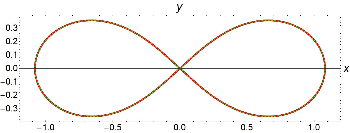
Figure 1: Trajectory of the Simo’s figure-eight 3-body system Simo02 . In this plot, we set $m=1$.

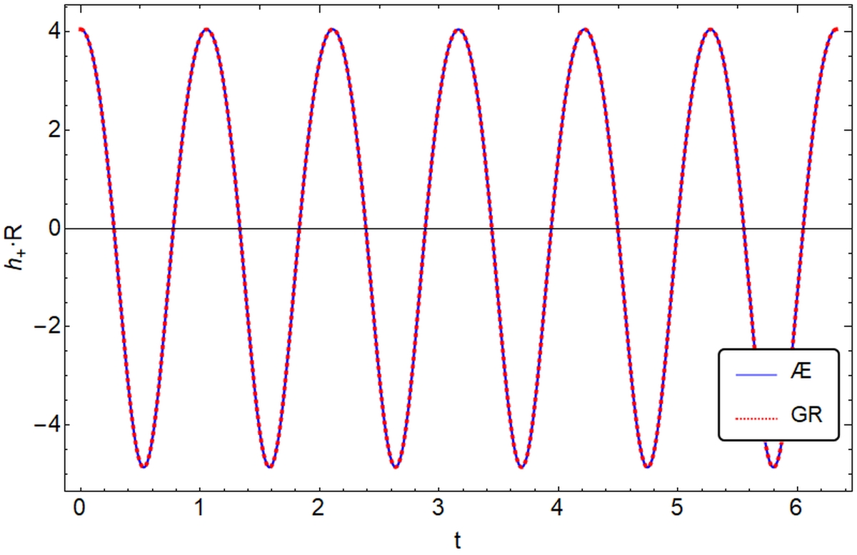
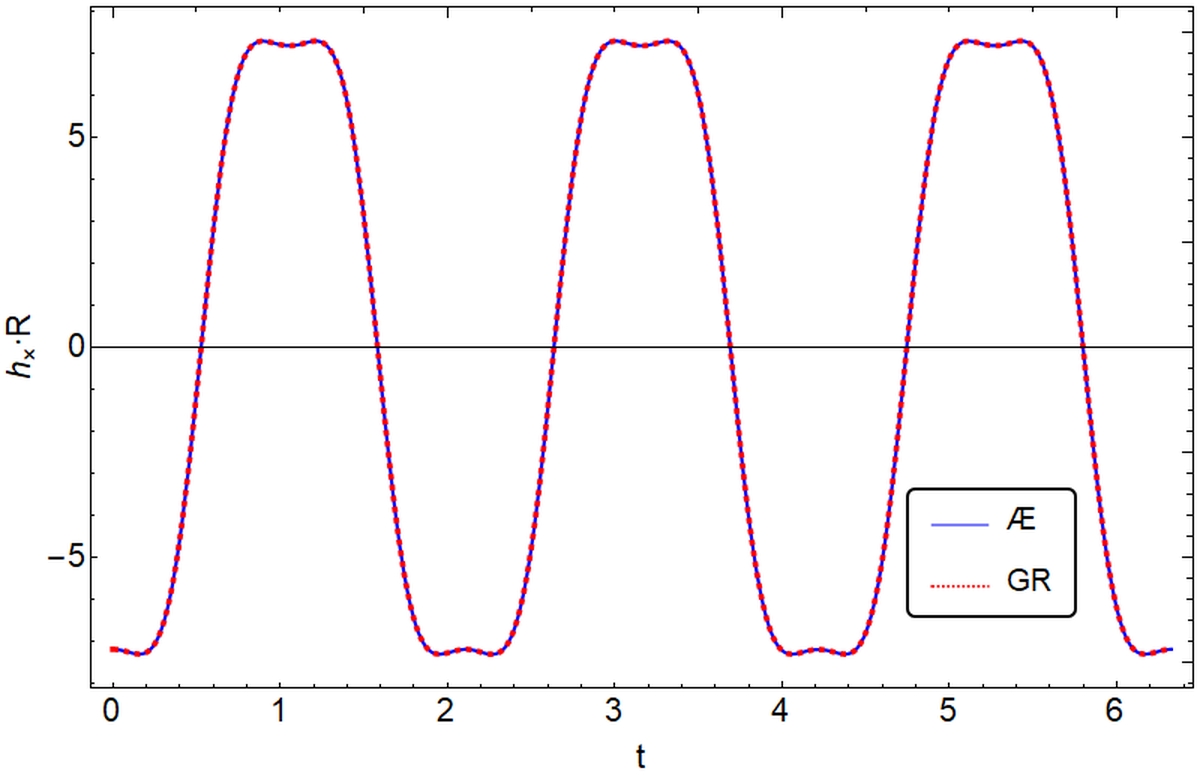
Figure 2: The polarization modes $h_{+}$ and $h_{\times}$ defined in Eq.(IV.1) for the Simo’s figure-eight 3-body system in both GR and $\ae$-theory, where the modes are propagating along the positive $z$-direction, and $(\Omega_{1},\;\Omega_{2},\;\Omega_{3})=(-0.1,\;-2.76\times 10^{-6},\;-2.9\times 10^{-5})$.

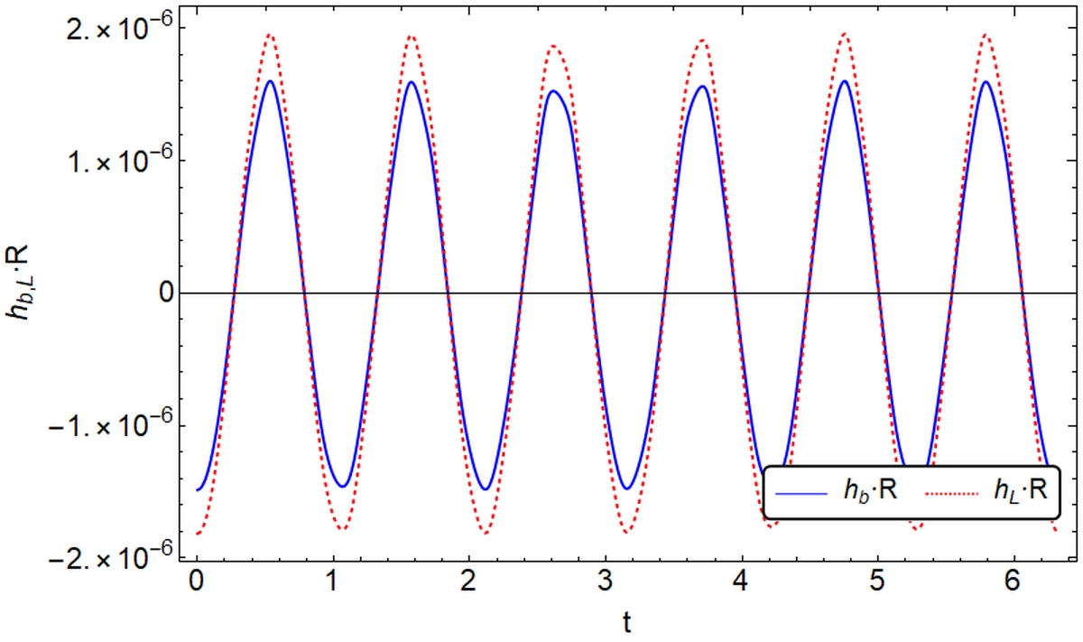
Figure 3: The polarization modes $h_{b}$ and $h_{L}$ defined in Eq.(IV.1) for the Simo’s figure-eight 3-body system in $\ae$-theory, where the modes are propagating along the positive $z$-direction., and $(\Omega_{1},\;\Omega_{2},\;\Omega_{3})=(-0.1,\;-2.76\times 10^{-6},\;-2.9\times 10^{-5})$.

In this paper, we shall consider some of the trajectories provided in Website .

Before doing so, let us first consider the GW form of the Simo’s figure-eight trajectory Simo02 , studied in DSH14 . In Fg. 1, the trajectory of the 3-body problem is plotted out in the ($x,y$)-plane for many periods, in order to make sure that our numerical codes converge well after a sufficiently long run. Assuming that the detector is along the $z$-axis, we plot out the polarization modes $h_{+}$ and $h_{\times}$ in Fig. 2. In this figure, we plot these modes given in GR as well as in Einstein-aether theory. As we noted previously, the contributions from the aether field is of the order of ${\cal{O}}\left(10^{-5}\right)$ lower than that of GR. This can be seen clearly from this figure, in which the lines are almost identical in both of theories. Note that when plotting these figures, we assumed that the binding energies of the three bodies are, respectively, $\Omega_{1}=-0.1,\;\Omega_{2}=-2.76\times 10^{-6}$ and $\Omega_{1}=-2.9\times 10^{-5}$, which are the same as these given for the PRS J0337+ 1715 Ransom14 , although here the three masses are assumed to be equal.

In Fig. 3 we plot out the polarization modes $h_{b}$ and $h_{L}$ in $\ae$-theory, which all vanish in GR. Comparing it with Fig. 2 it can be seen that the amplitudes of these modes are about five orders lower than $h_{+}$ and $h_{\times}$, which is again consistent with our analysis given in Sec. III.

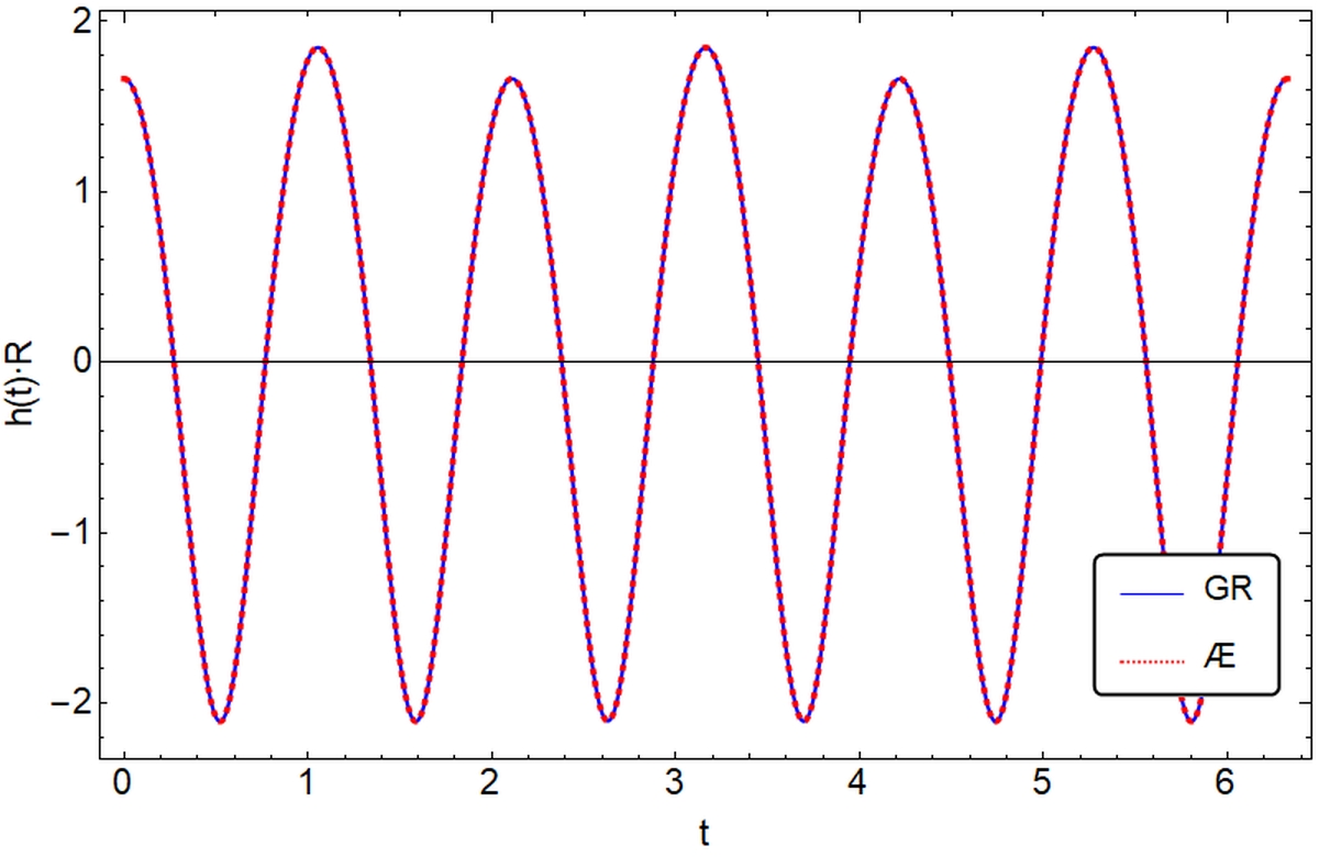
Figure 4: The response function $h(t)$ for the Simo’s figure-eight 3-body system in GR and $\ae$-theory, where the modes are propagating along the positive $z$-direction, and $(\Omega_{1},\;\Omega_{2},\;\Omega_{3})=(-0.1,\;-2.76\times 10^{-6},\;-2.9\times 10^{-5})$.

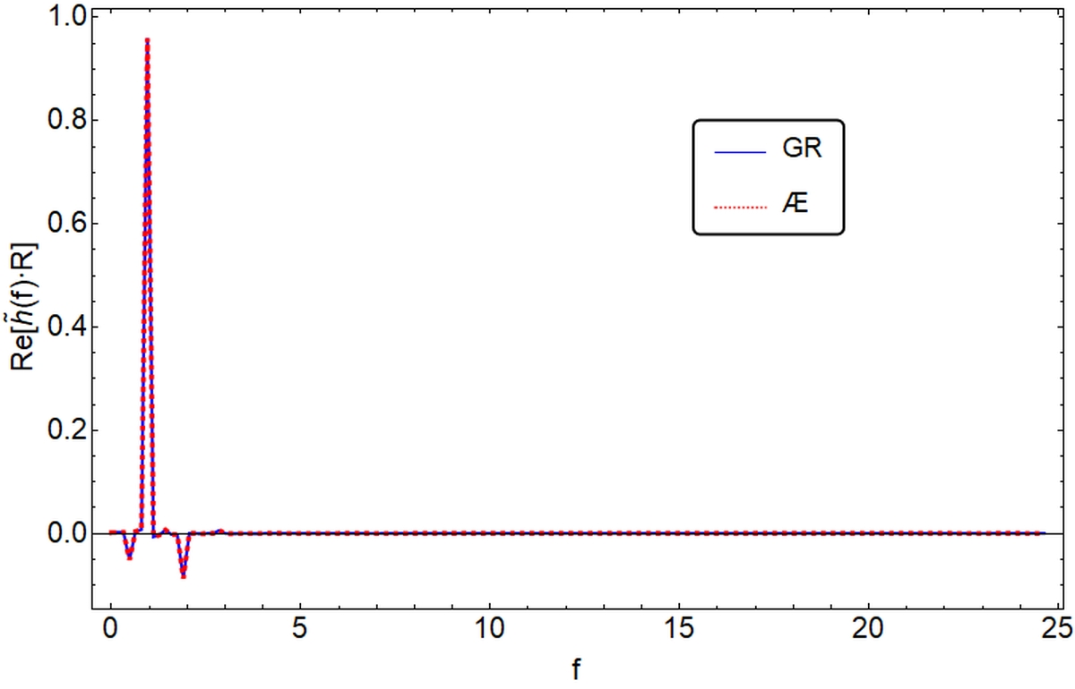
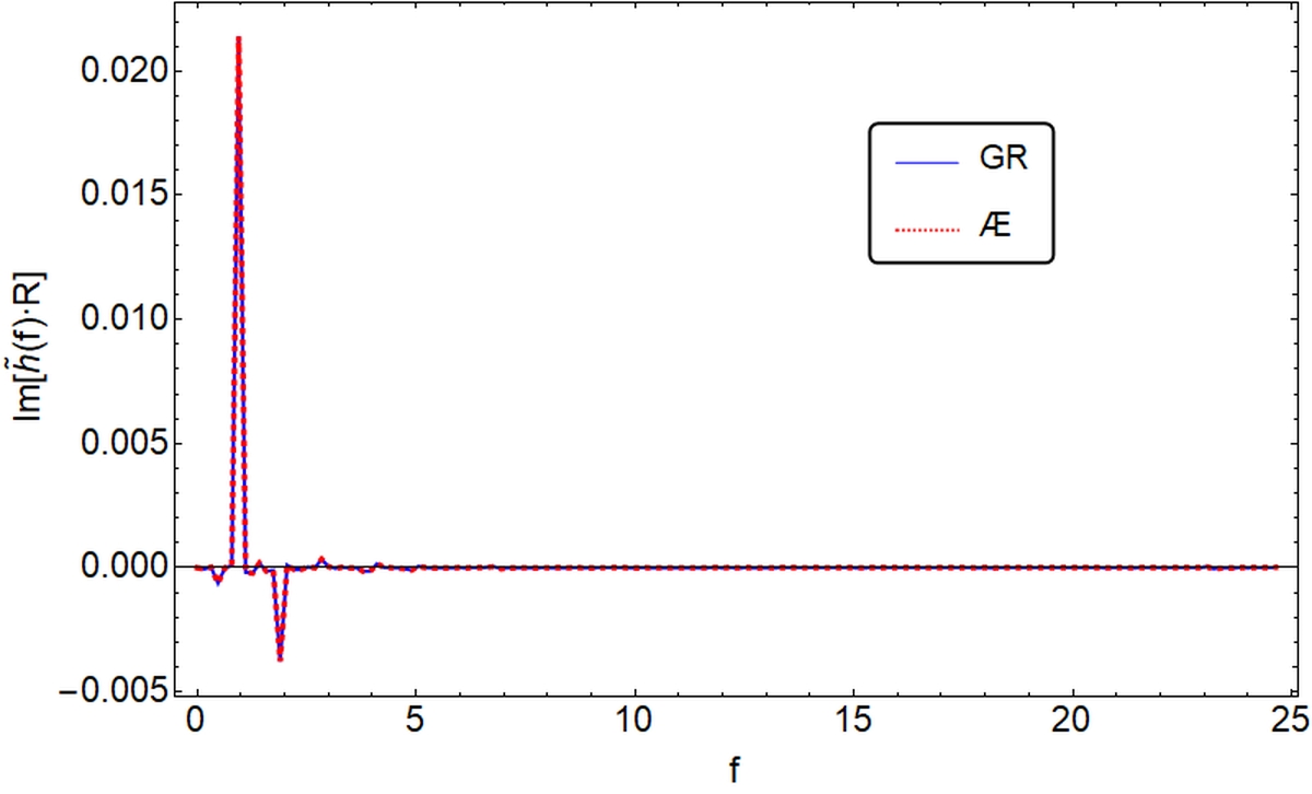
Figure 5: The Fourier transform $\tilde{h}(f)$ of the response function $h(t)$ for the Simo’s figure-eight 3-body system in GR and $\ae$-theory, where the modes are propagating along the positive $z$-direction, and $(\Omega_{1},\;\Omega_{2},\;\Omega_{3})=(-0.1,\;-2.76\times 10^{-6},\;-2.9\times 10^{-5})$.

Figure 6: The radiation power $P(\equiv-\dot{\cal{E}})$ of the Simo’s figure-eight 3-body system in $\ae$-theory, where the modes are all propagating along the positive $z$-direction, and $(\Omega_{1},\;\Omega_{2},\;\Omega_{3})=(-0.1,\;-2.76\times 10^{-6},\;-2.9\times 10^{-5})$. The dotted (blue), dash-dotted (red) and solid (green) lines denote, respectively, the parts of quadrupole, monopole and dipole radiations given in Eq.(3.1).

In Figs. 4, 5 and 6, we plot out the corresponding response function $h(t)$, its Fourier transform $\tilde{h}(f)$ and the radiation power $P(\equiv-\dot{\cal{E}})$ for the Simo’s figure-eight 3-body system. From Fig. 6 we can see that both of the dipole and monopole contributions are suppressed with the orders given in Section III.

Note that in drawing the above figures, we had set $c_{1}=4\times 10^{-5},c_{2}=9\times 10^{-5},c_{3}=-c_{1}$, and $c_{4}=-2\times 10^{-5}$, a condition that will be adopted for the rest of this paper. For such choices, the coupling constants $c_{i}$’s clearly satisfy the theoretical and observational constraints of the $\ae$-theory OMW18 , given by Eq.(2.18).

In addition, with these choices, we have $c_{13}=0$, and then from Eq.(IV.1) we find that the vectorial modes $h_{X}$ and $h_{Y}$ are identically zero,

$$h_{X}=h_{Y},\;(c_{13}=0).$$ (5.7)

So, in the rest of this paper we only need to consider the $h_{+},\;h_{\times},\;h_{b}$ and $h_{L}$ modes.

Yet, we also plot the above figures by assuming that the orbit is in the ($x,y$)-plane, while the detector is along the $z$-axis. The same conditions were also assumed in DSH14 . However, as we mentioned in the last section, the locations and orientations of the sources as well as the detectors are all independent, which are specified by the five angles $(\vartheta,\varphi;\theta,\phi,\psi)$, defined in Eqs.(IV.1) and (IV.2). For different choices of these parameters, the wave forms and response function will be also different. In Figs. 7-11 we plot the mode functions $h_{N}$, response function $h(t)$, its Fourier transform $\tilde{h}(f)$ and the radiation powers $P_{{\cal{A}}}$, $P_{{\cal{B}}}$ and $P_{{\cal{C}}}$, respectively, for $(\vartheta,\varphi;\theta,\phi,\psi)=(0.6,5.2;1.3,1.2,1.8)$, while still chose $(\Omega_{1},\;\Omega_{2},\;\Omega_{3})=(-0.1,\;-2.76\times 10^{-6},\;-2.9\times 10^{-5})$. Clearly, the corresponding mode functions, response function and its Fourier transform are all different from the case in which the 3-bodies are in the $(x,y$)-plane, while the detector is localized along the $z$-axis. However, the radiation powers are the same and are independent of the choice of these five angular parameters, as can be seen from Figs. 6 and 11.

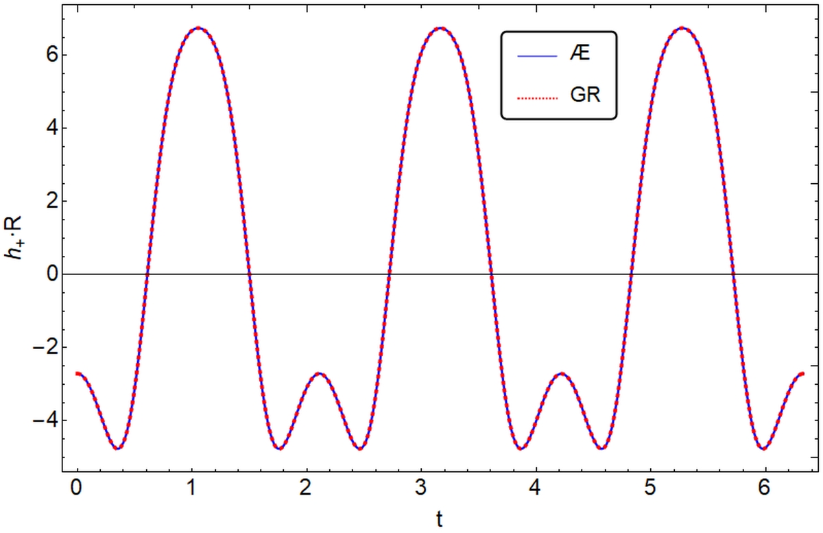
Figure 7: The polarization modes $h_{+}$ and $h_{\times}$ defined in Eq.(IV.1) for the Simo’s figure-eight 3-body system in both GR and $\ae$-theory, where the modes are propagating along the direction specified by $(\vartheta,\varphi;\theta,\phi,\psi)=(0.6,5.2;1.3,1.2,1.8)$ with $\left(\Omega_{1},\;\Omega_{2},\;\Omega_{3})=(-0.1,\;-2.76\times 10^{-6},\;-2.9\times 10^{-5}\right)$.

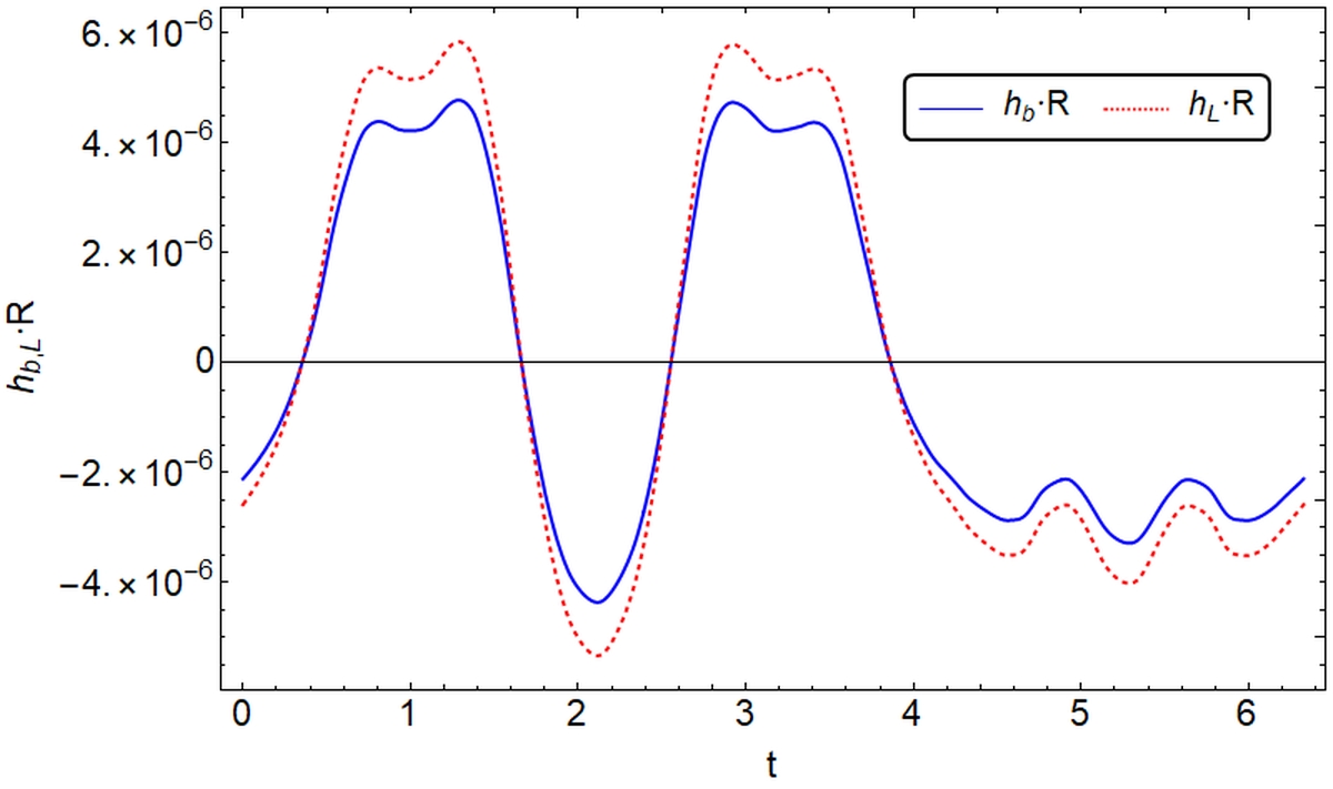
Figure 8: The polarization modes $h_{b}$ and $h_{L}$ defined in Eq.(IV.1) for the Simo’s figure-eight 3-body system in $\ae$-theory, where the modes are propagating along the direction specified by $(\vartheta,\varphi;\theta,\phi,\psi)=(0.6,5.2;1.3,1.2,1.8)$ with $\left(\Omega_{1},\;\Omega_{2},\;\Omega_{3})=(-0.1,\;-2.76\times 10^{-6},\;-2.9\times 10^{-5}\right)$.

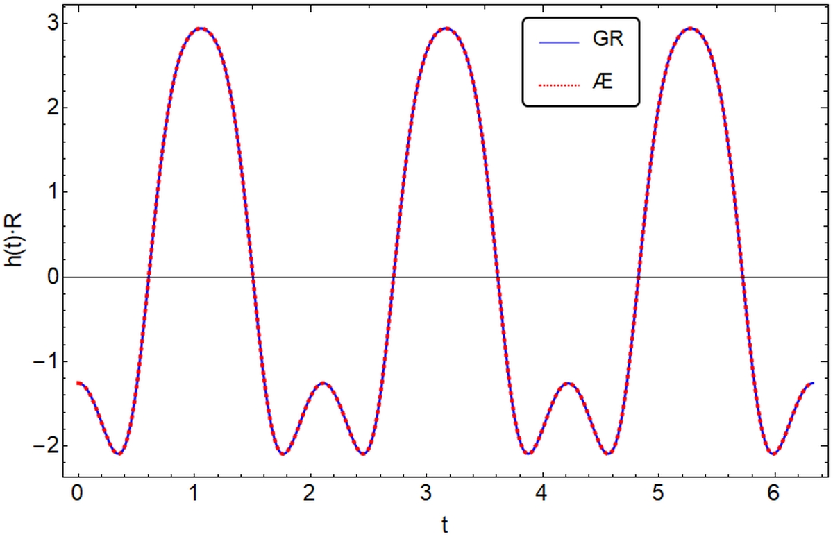
Figure 9: The response function $h(t)$ for the Simo’s figure-eight 3-body system in GR and $\ae$-theory, where the modes are propagating along the direction specified by $(\vartheta,\varphi;\theta,\phi,\psi)=(0.6,5.2;1.3,1.2,1.8)$ with $\left(\Omega_{1},\;\Omega_{2},\;\Omega_{3})=(-0.1,\;-2.76\times 10^{-6},\;-2.9\times 10^{-5}\right)$.

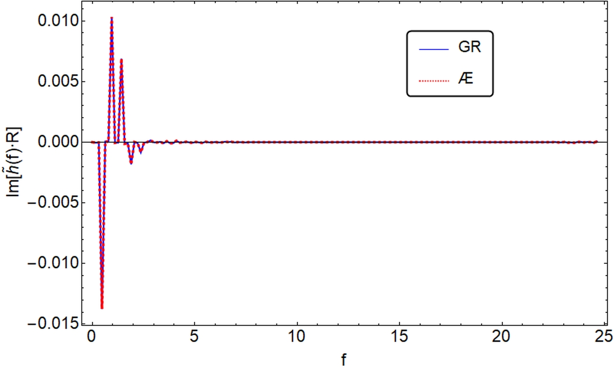
Figure 10: The Fourier transform $\tilde{h}(f)$ of the response function $h(t)$ for the Simo’s figure-eight 3-body system in GR and $\ae$-theory, where the modes are propagating along the direction specified by $(\vartheta,\varphi;\theta,\phi,\psi)=(0.6,5.2;1.3,1.2,1.8)$ with $\left(\Omega_{1},\;\Omega_{2},\;\Omega_{3})=(-0.1,\;-2.76\times 10^{-6},\;-2.9\times 10^{-5}\right)$.

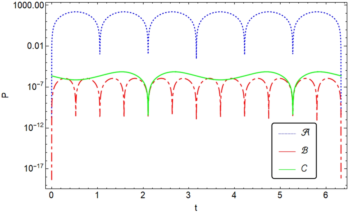
Figure 11: The radiation power $P(\equiv-\dot{\cal{E}})$ of the Simo’s figure-eight 3-body system in $\ae$-theory, where the modes are propagating along the direction specified by $(\vartheta,\varphi;\theta,\phi,\psi)=(0.6,5.2;1.3,1.2,1.8)$ with $\left(\Omega_{1},\;\Omega_{2},\;\Omega_{3})=(-0.1,\;-2.76\times 10^{-6},\;-2.9\times 10^{-5}\right)$. The dotted (blue), dash-dotted (red) and solid (green) lines denote, respectively, the parts of quadrupole, monopole and dipole radiations given in Eq.(3.1).

To study the effects of the binding energies of the three bodies on the wave forms and energy losses, let us consider the same case as shown by Figs. 7 - 11 but now with the same binding energy, $\Omega_{a}=-10^{-2}$. With this choice, the dipole contributions are identically zero, as one can see from Eqs.(V) and (V), since now we have ${\cal D}_{c}=0,\;(c=1,2,3)$ and $\dot{\Sigma}_{i}^{2}=0$. This does not contradict with the results given by Eq.(III), as there we assumed that $\Omega_{1}/m_{1}-\Omega_{2}/m_{2}\simeq{\cal{O}}\left(\Omega/m\right)$ [cf. Eqs.(3.6) and (III)]. But, here due to our choice of $\Omega_{a}$ and $m_{a}$, we have $\Omega_{1}/m_{1}-\Omega_{2}/m_{2}=0$ and so on. In Figs. 12 - 16 we plot the mode functions $h_{N}$, response function $h(t)$, its Fourier transform $\tilde{h}(f)$ and the radiation powers $P_{{\cal{A}}}$ and $P_{{\cal{B}}}$, respectively, for $(\vartheta,\varphi;\theta,\phi,\psi)=(0.6,5.2;1.3,1.2,1.8)$, while setting $(\Omega_{1},\;\Omega_{2},\;\Omega_{3})=(-10^{-2},-10^{-2},-10^{-2})$. Clearly, the corresponding mode functions, response function, its Fourier transform and radiation powers are all different from the case in which the 3-bodies are in the $(x,y$)-plane, while the detector is localized along the $z$-axis. In particular, the dipole contributions vanish now, as explained above.

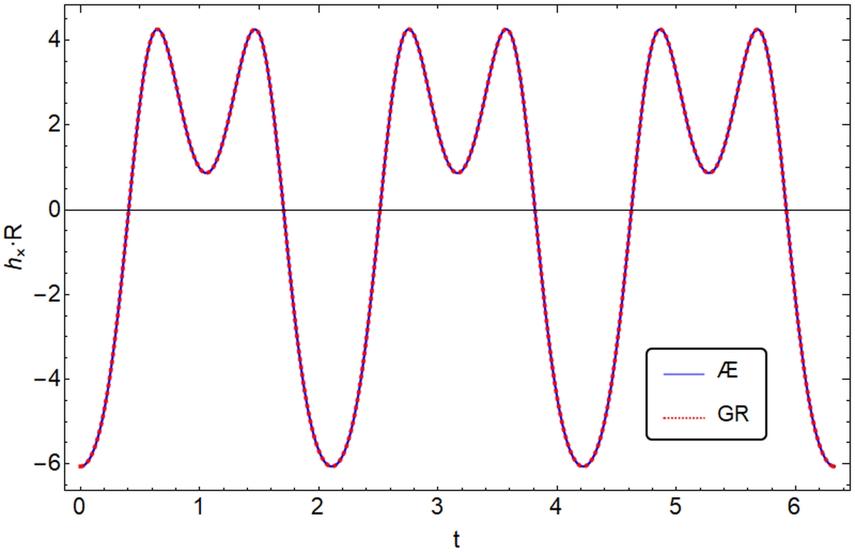
Figure 12: The polarization modes $h_{+}$ and $h_{\times}$ defined in Eq.(IV.1) for the Simo’s figure-eight 3-body system in both GR and $\ae$-theory, where the modes are propagating along the direction specified by $(\vartheta,\varphi;\theta,\phi,\psi)=(0.6,5.2;1.3,1.2,1.8)$, with $\Omega_{1}=\Omega_{2}=\Omega_{3}=-10^{-2}$.

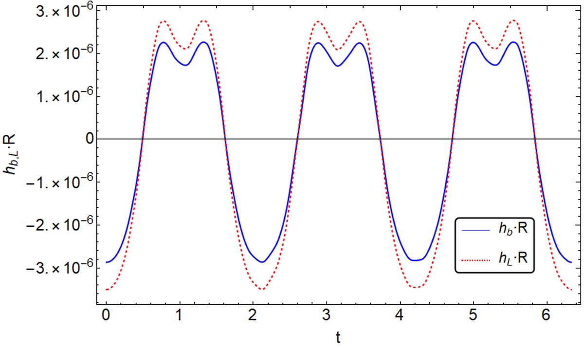
Figure 13: The polarization modes $h_{b}$ and $h_{L}$ defined in Eq.(IV.1) for the Simo’s figure-eight 3-body system in $\ae$-theory, where the modes are propagating along the direction specified by $(\vartheta,\varphi;\theta,\phi,\psi)=(0.6,5.2;1.3,1.2,1.8)$, with $\Omega_{1}=\Omega_{2}=\Omega_{3}=-10^{-2}$.

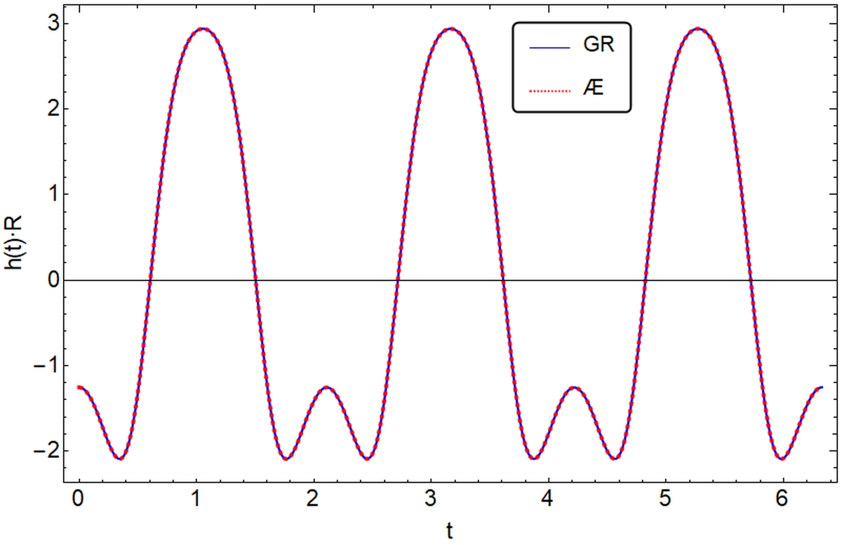
Figure 14: The response function $h(t)$ for the Simo’s figure-eight 3-body system in GR and $\ae$-theory, where the modes are propagating along the direction specified by $(\vartheta,\varphi;\theta,\phi,\psi)=(0.6,5.2;1.3,1.2,1.8)$, with $\Omega_{1}=\Omega_{2}=\Omega_{3}=-10^{-2}$.

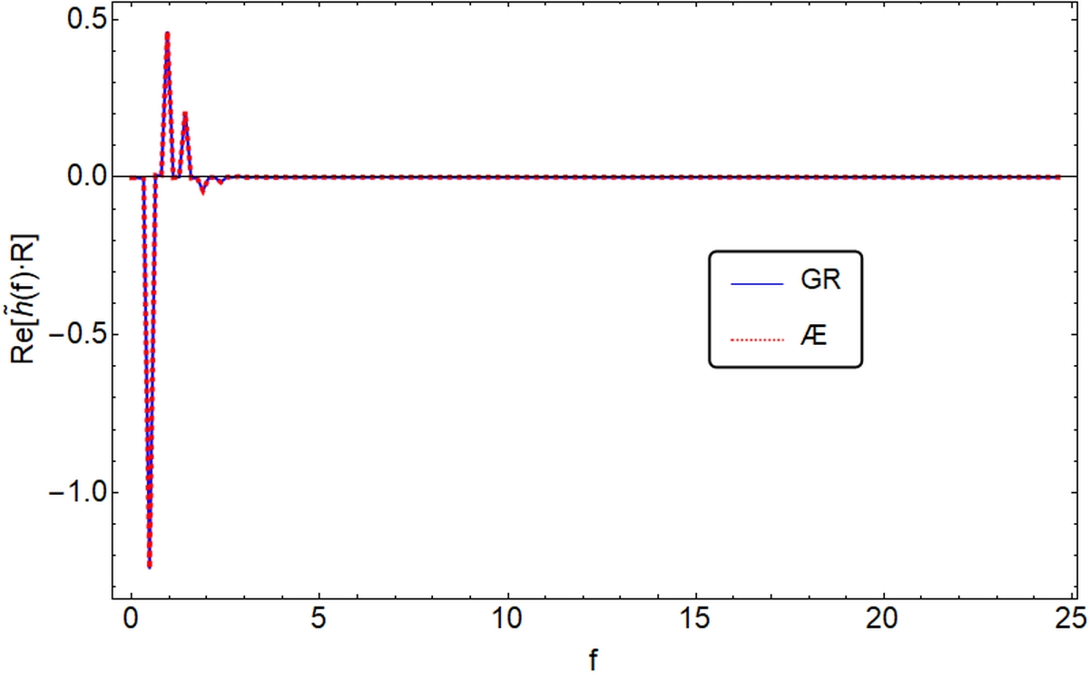
Figure 15: The Fourier transform $\tilde{h}(f)$ of the response function $h(t)$ for the Simo’s figure-eight 3-body system in GR and $\ae$-theory, where the modes are propagating along the direction specified by $(\vartheta,\varphi;\theta,\phi,\psi)=(0.6,5.2;1.3,1.2,1.8)$, with $\Omega_{1}=\Omega_{2}=\Omega_{3}=-10^{-2}$.

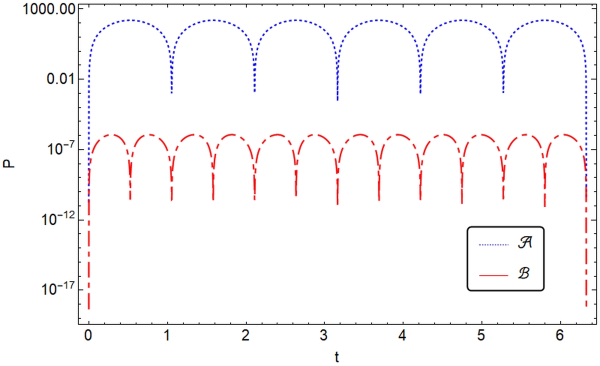
Figure 16: The radiation power $P(\equiv-\dot{\cal{E}})$ of the Simo’s figure-eight trajectory of 3-body system in GR and $\ae$-theory, where the modes are propagating along the direction specified by $(\vartheta,\varphi;\theta,\phi,\psi)=(0.6,5.2;1.3,1.2,1.8)$, with $\Omega_{1}=\Omega_{2}=\Omega_{3}=-10^{-2}$. The dotted (blue) and solid (red) lines denote, respectively, the parts of quadrupole and monopole radiations given in Eq.(3.1). Because of the choice of the binding energies $\Omega_{a}$ and masses $m_{a}$ are all the same for the three compact objects, the dipole contributions, denoted by the ${\cal{C}}$ part in Eq.(3.1), are identically zero.

In Figs. 17-21, we plot out, respectively, the trajectory of the Broucke R7 3-body system provided in Website , the polarization modes $h_{N}$, the response function $h(t)$, its Fourier transform $\tilde{h}(f)$ and the radiation powers $P_{{\cal{A}}}$, $P_{{\cal{B}}}$ and $P_{{\cal{C}}}$, for $(\vartheta,\varphi;\theta,\phi,\psi)=(0.6,5.2;1.3,1.2,1.8)$, and $(\Omega_{1},\;\Omega_{2},\;\Omega_{3})=(-0.1,\;-2.76\times 10^{-6},\;-2.9\times 10^{-5})$.

In Fig. 22 we plot out the trajectory of the Broucke A16 3-body system provided in Website , while in Fig. 23-26 we plot out the corresponding physical quantities for the same choice of the five angular parameters as selected in the case for the Broucke R7 3-body system in both GR and $\ae$-theory with $(\Omega_{1},\;\Omega_{2},\;\Omega_{3})=(-0.1,\;-2.76\times 10^{-6},\;-2.9\times 10^{-5})$.

From these figures we can see clearly that the GW forms and radiation powers not only depend on the relative positions, orientations between the source and detector, but also depend on the configurations of the orbits of the 3-body system. In addition, they also depend on their binding energies of the three compact bodies.

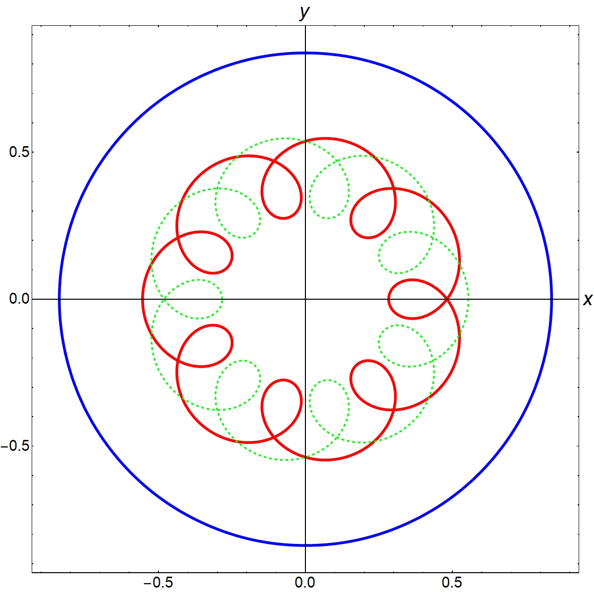
Figure 17: Trajectory of the 3-body system for the Broucke R7 figure provided in Website .

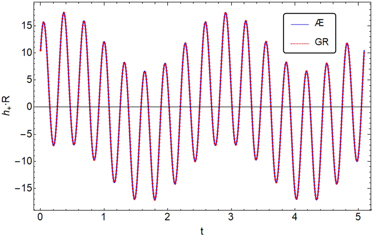
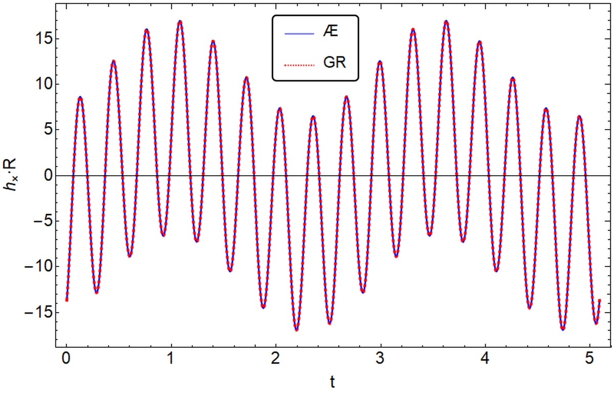
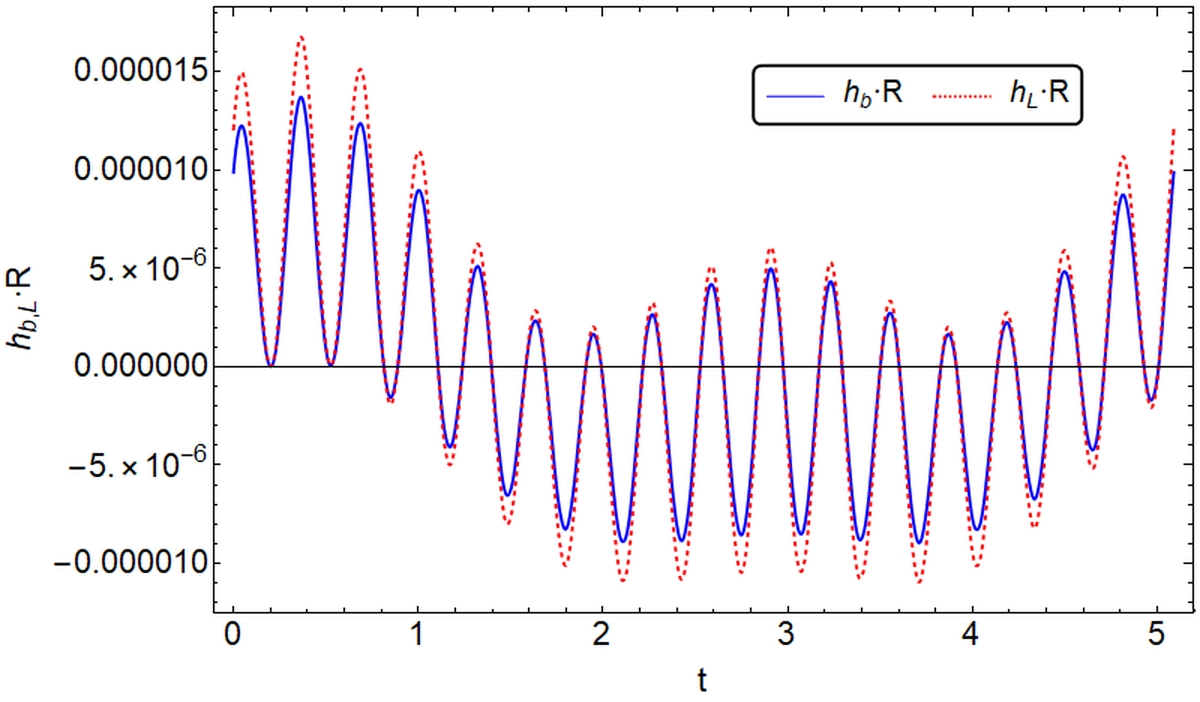
Figure 18: The polarization modes $h_{N}$ defined in Eq.(IV.1) for the Broucke R7 3-body system with the choice, $(\vartheta,\varphi;\theta,\phi,\psi)=(0.6,5.2;1.3,1.2,1.8)$ and $(\Omega_{1},\;\Omega_{2},\;\Omega_{3})=(-0.1,\;-2.76\times 10^{-6},\;-2.9\times 10^{-5})$.

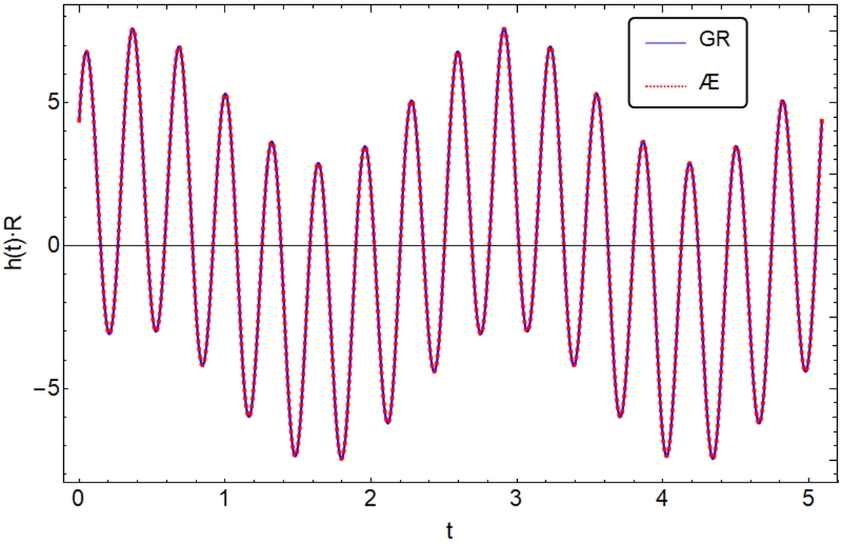
Figure 19: The response function $h(t)$ for the Broucke R7 3-body system with the choice, $(\vartheta,\varphi;\theta,\phi,\psi)=(0.6,5.2;1.3,1.2,1.8)$ and $(\Omega_{1},\;\Omega_{2},\;\Omega_{3})=(-0.1,\;-2.76\times 10^{-6},\;-2.9\times 10^{-5})$.

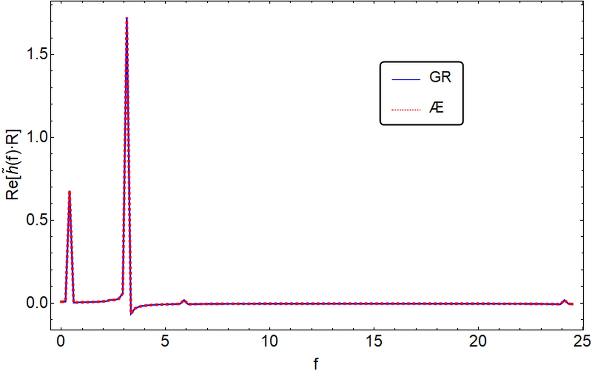
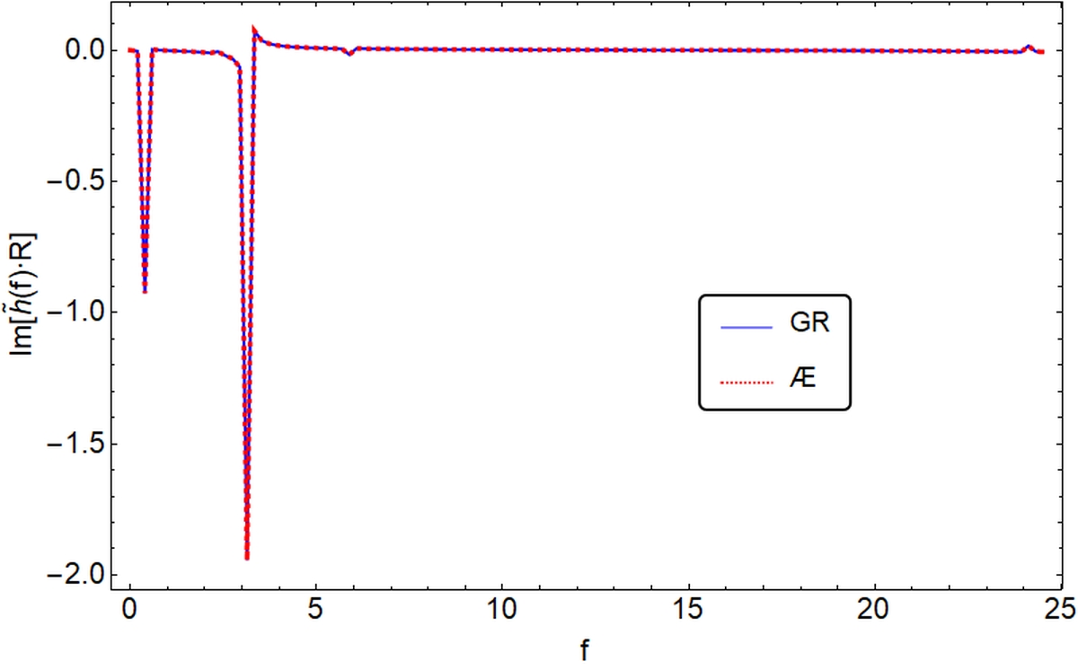
Figure 20: The Fourier transform $\tilde{h}(f)$ of the response function $h(t)$ for the Broucke R7 3-body system with the choice, $(\vartheta,\varphi;\theta,\phi,\psi)=(0.6,5.2;1.3,1.2,1.8)$ and $(\Omega_{1},\;\Omega_{2},\;\Omega_{3})=(-0.1,\;-2.76\times 10^{-6},\;-2.9\times 10^{-5})$.

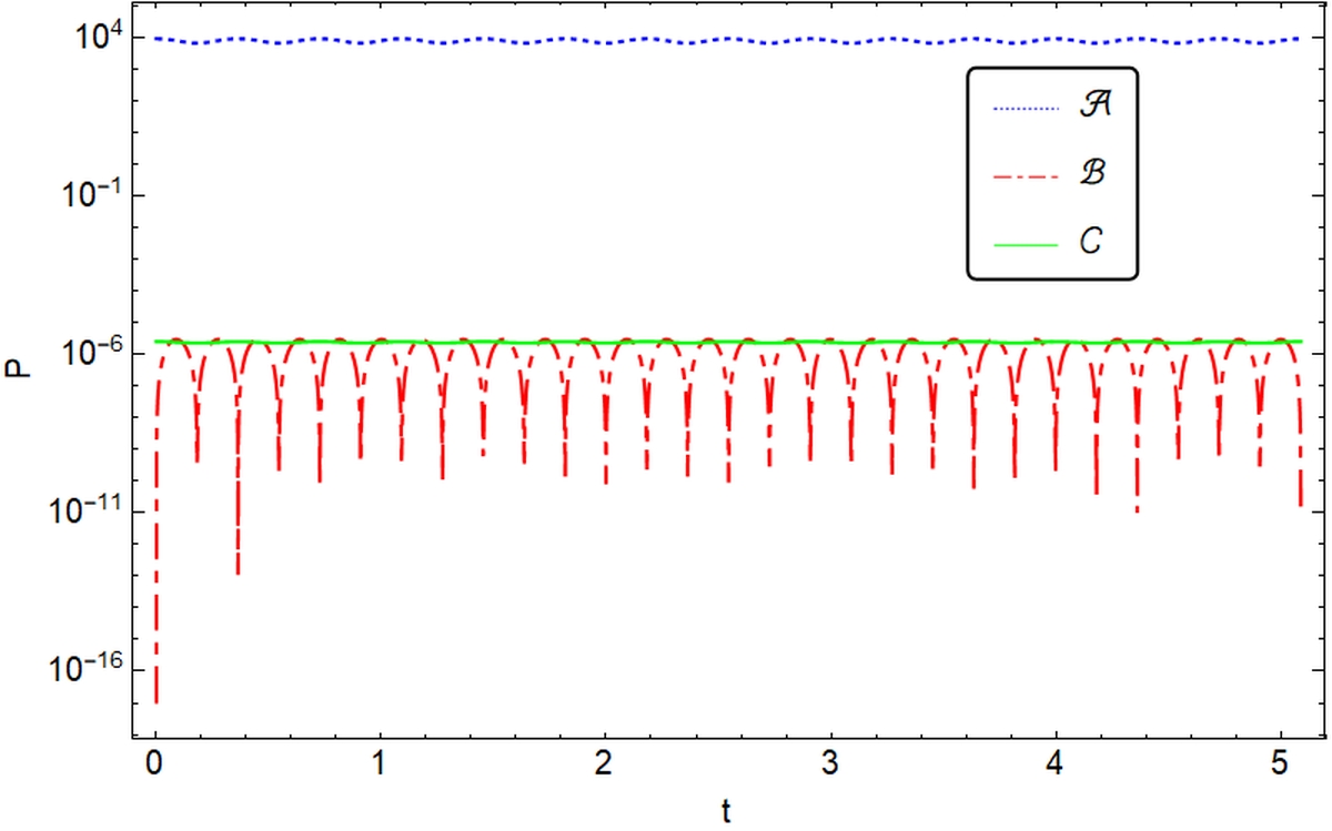
Figure 21: The radiation power $P(\equiv-\dot{\cal{E}})$ of the 3-body system of the Broucke R7 figure with the choice, $(\vartheta,\varphi;\theta,\phi,\psi)=(0.6,5.2;1.3,1.2,1.8)$ and $(\Omega_{1},\;\Omega_{2},\;\Omega_{3})=(-0.1,\;-2.76\times 10^{-6},\;-2.9\times 10^{-5})$. The dotted (blue), dash-dotted (red) and solid (green) lines denote, respectively, the parts of quadrupole, monopole and dipole radiations given in Eq.(3.1).

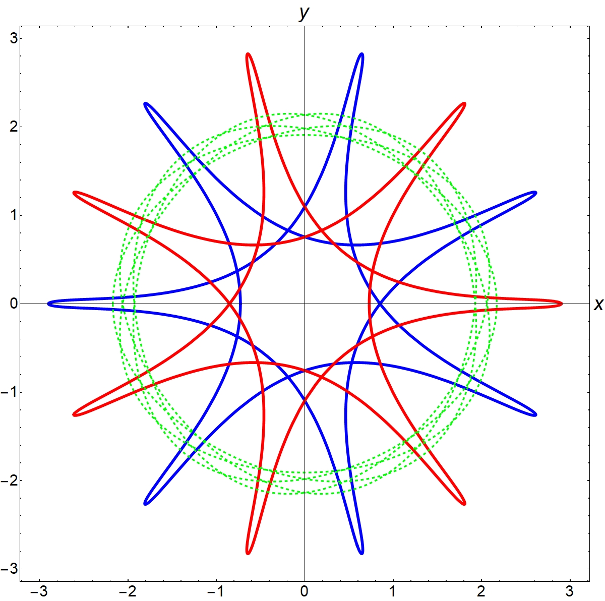
Figure 22: Trajectory of the 3-body system for the Broucke A16 figure provided in Website .

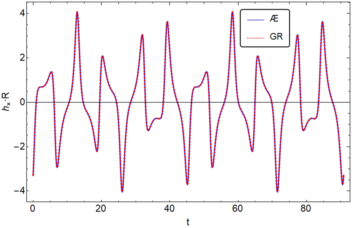
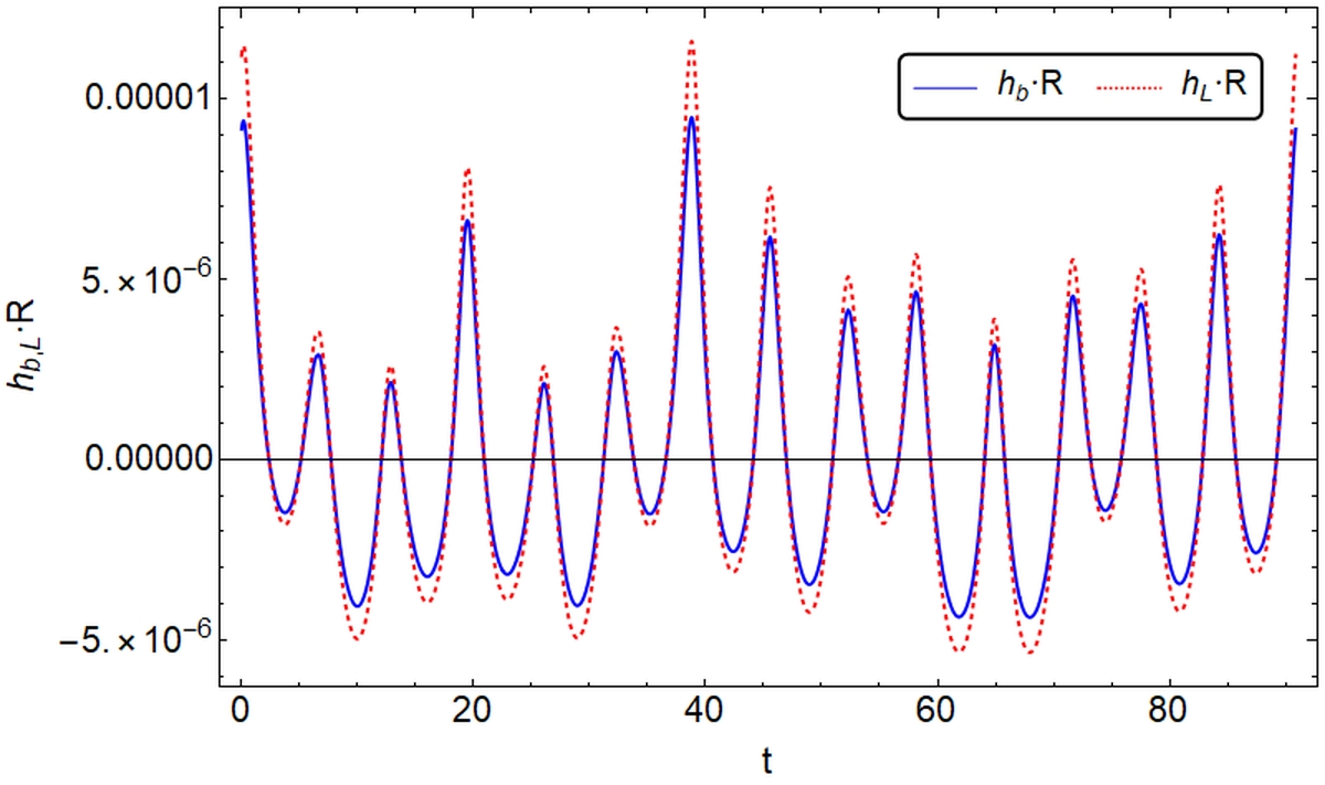
Figure 23: The polarization modes $h_{N}$ defined in Eq.(IV.1) for the Broucke A16 3-body system with the choice, $(\vartheta,\varphi;\theta,\phi,\psi)=(0.6,5.2;1.3,1.2,1.8)$ and $(\Omega_{1},\;\Omega_{2},\;\Omega_{3})=(-0.1,\;-2.76\times 10^{-6},\;-2.9\times 10^{-5})$.

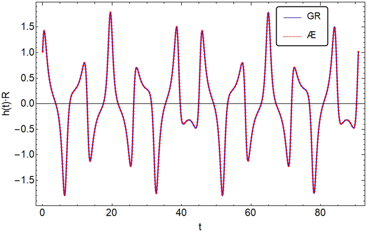
Figure 24: The response function $h(t)$ for the Broucke A16 3-body system with the choice, $(\vartheta,\varphi;\theta,\phi,\psi)=(0.6,5.2;1.3,1.2,1.8)$ and $(\Omega_{1},\;\Omega_{2},\;\Omega_{3})=(-0.1,\;-2.76\times 10^{-6},\;-2.9\times 10^{-5})$.

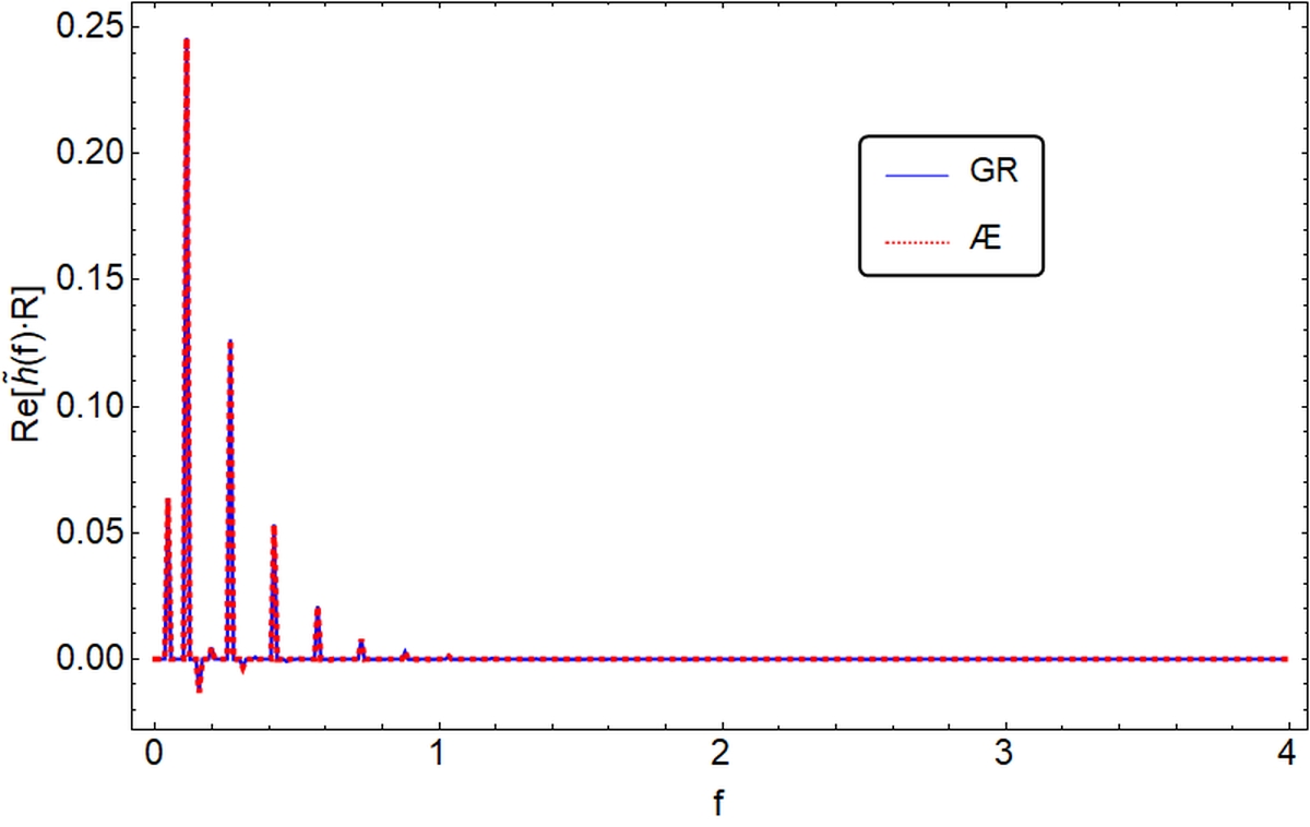
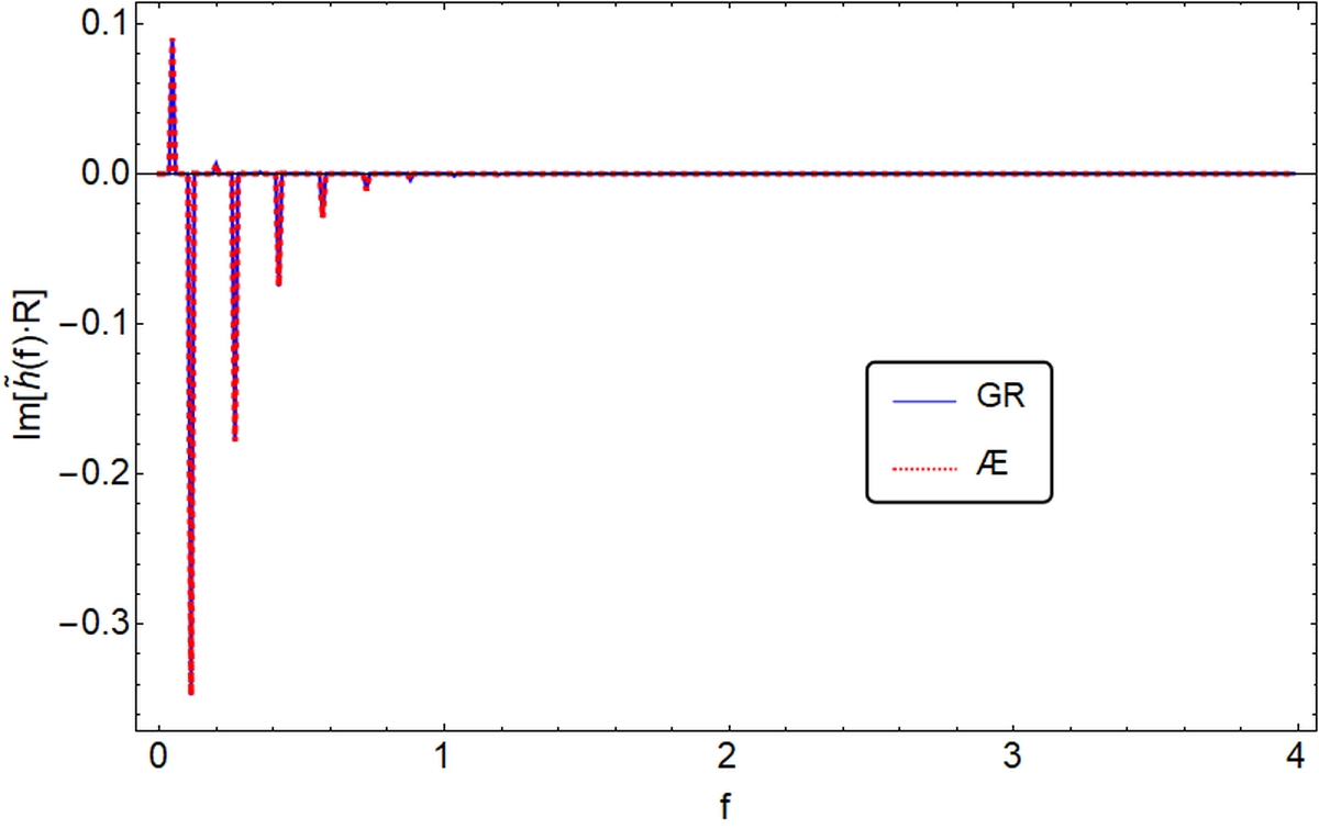
Figure 25: The Fourier transform $\tilde{h}(f)$ of the response function $h(t)$ for the Broucke A16 3-body system with the choice, $(\vartheta,\varphi;\theta,\phi,\psi)=(0.6,5.2;1.3,1.2,1.8)$ and $(\Omega_{1},\;\Omega_{2},\;\Omega_{3})=(-0.1,\;-2.76\times 10^{-6},\;-2.9\times 10^{-5})$.

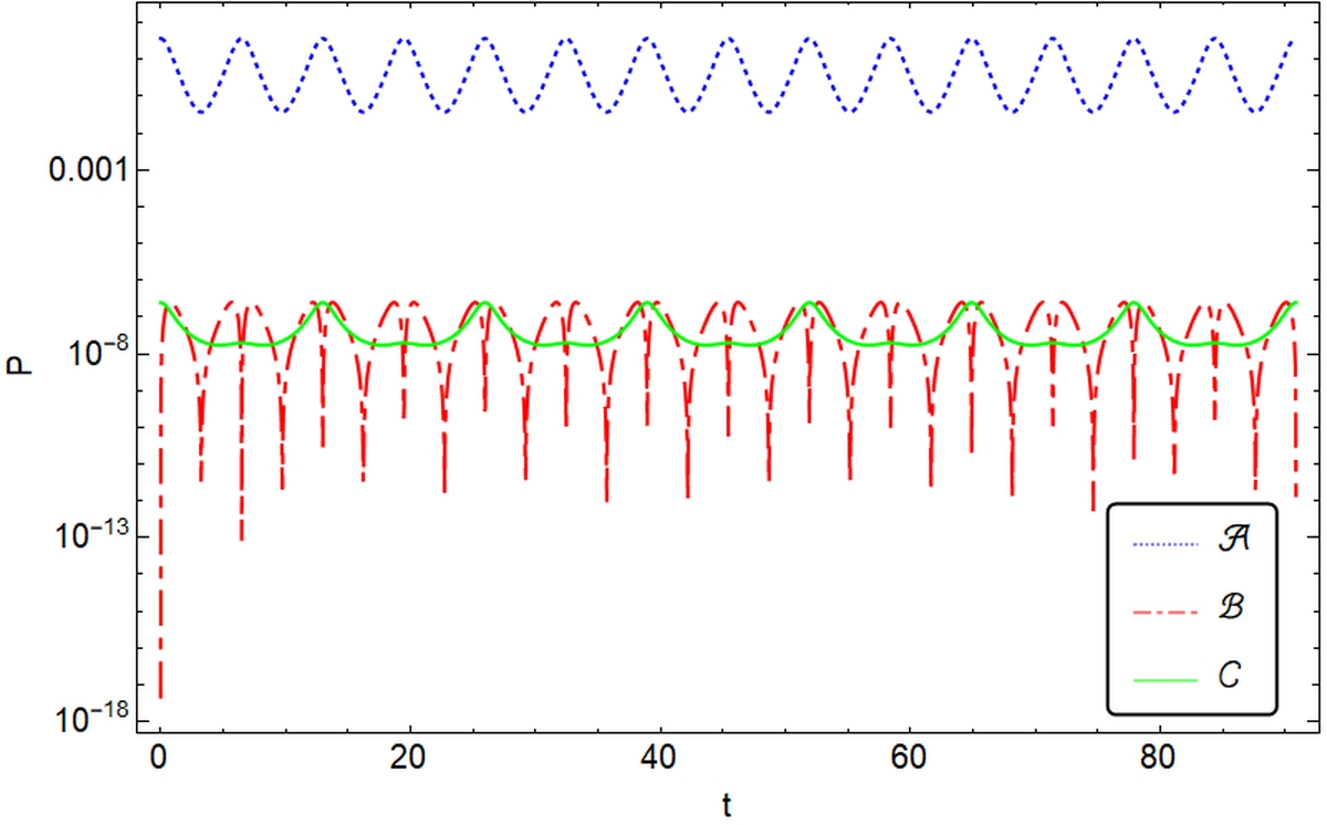
Figure 26: The radiation power $P(\equiv-\dot{\cal{E}})$ of the 3-body system of the Broucke A16 figure with the choice, $(\vartheta,\varphi;\theta,\phi,\psi)=(0.6,5.2;1.3,1.2,1.8)$ and $(\Omega_{1},\;\Omega_{2},\;\Omega_{3})=(-0.1,\;-2.76\times 10^{-6},\;-2.9\times 10^{-5})$. The dotted (blue), dash-dotted (red) and solid (green) lines denote, respectively, the parts of quadrupole, monopole and dipole radiations given in Eq.(3.1).

VI Conclusions

Three-body systems have been attracting more and more attention recently Naoz16 , specially after the detections of GWs from binary systems GW150914 ; GW151226 ; GW170104 ; GW170608 ; GW170814 ; GW170817 , as they are common in our Universe FC17 , and can be ideal sources for periodic GWs. In particular, we are very much interested in the cases in which the orbits of two bodies pass each other very closely and yet avoid collisions, so they can produce intense periodic gravitational waves and provide natural sources for the future detections of GWs.

In this paper, we have studied the lowest PN order of three-body problems in the framework of Einstein-aether theory Jacobson , a theory that violates locally the Lorentz symmetry and yet passes all the theoretical and observational tests carried out so far OMW18 . Although these tests were mainly in the weak field limits, strong-field effects of binary neutron stars systems have been also investigated Foster07 ; Yagi14 ; HYY15 ; SY18 . In particular, the accelerations and “strong-field” Nordtvedt parameter were calculated recently for a triple system to the quasi-Newtonian order Will18 .

In this paper, we have first shown that the contributions of the presence of the aether field to the quadruple part of the energy loss rate of a binary system is the order of ${\cal{O}}\left(c_{14}\right)\lesssim{\cal{O}}\left(10^{-5}\right)$ lower than that of GR when only the lowest PN order is taken into account [cf. Eq.(III)]. Due to the presence of two additional modes, the scalar and vector, in Einstein-aether theory, two additional parts also appear in the energy loss rate of a binary system Foster06 , given respectively by the second and third terms in Eq.(3.1), representing the monopole and dipole contributions. In comparison with the quadruple contributions of GR, which is the order of ${\cal{O}}\left(v^{2}\right)$, the monopole contributions is only of the order of ${\cal{O}}\left(c_{14}\right){\cal{O}}\left(v^{2}\right)$, that is, it is about ${\cal{O}}\left(c_{14}\right)\lesssim{\cal{O}}\left(10^{-5}\right)$ order lower than that of GR. Here $v$ is the relative velocity of the two compact objects. However, the dipole contributions can be much larger than those of monopole. In particular, for a binary system with large differences between their binding energies, the dipole part can be as large as ${\cal{O}}\left(c_{14}\right){\cal{O}}\left(G_{N}m/d\right)$, where $m$ denotes the mass of a binary system and $d$ the distance between the two stars. For a realistic neutron star, we have ${\cal{O}}\left(G_{N}m/d\right)\simeq 0.1\sim 0.3$, so that ${\cal{O}}\left(c_{14}\right){\cal{O}}\left(G_{N}m/d\right)\simeq 10^{-2}{\cal{O}}\left(v^{2}\right)$. It should be noted that the scalar mode has contributions to all the three parts, quadrupole, dipole and monopole, while the vector mode has contributions only to the quadrupole and dipole parts, as can be seen clearly from Eqs.(102)-(104) of Ref. Foster06 . On the other hand, the strong-field contributions are only of the orders of

$$\delta{\cal{W}}^{\mathrm{NS}}_{\cal{A}} \lesssim {\cal{O}}\left(10^{{-11}}\right),\quad\delta{\cal{W}}^{\mathrm{NS}}_{\cal{B}}\lesssim{\cal{O}}\left(10^{{-11}}\right),$$

$$\delta{\cal{W}}^{\mathrm{NS}}_{\cal{C}} \lesssim {\cal{O}}\left(10^{{-12}}\right),\quad\delta{\cal{W}}^{\mathrm{NS}}_{\cal{D}}\lesssim{\cal{O}}\left(10^{{-11}}\right),$$ (6.1)

for a binary neutron star system, where $\delta{\cal{W}}^{\mathrm{NS}}_{\cal{A}},\;\delta{\cal{W}}^{\mathrm{NS}}_{\cal{B}}$ and $\delta{\cal{W}}^{\mathrm{NS}}_{\cal{C}}$ represent the contributions of the strong-field effects to the quadrupole, monopole and dipole parts of Eq.(3.1), while $\delta{\cal{W}}^{\mathrm{NS}}_{\cal{D}}$ denotes a cross term due to the motion of the center-of-mass of the system Yagi14 . Clearly, these effects are much smaller than the ones mentioned above, and are out of the detectability of the current generation of detectors.

So, in this paper we have ignored these effects, and simply set the sensitivities $s_{A}$ of the compact bodies to zero. However, in the development of the general formulas, we have kept $T_{\mu}$ not zero to its first-order of perturbations in Sec. IV, for our later applications of the formulas. Here $T_{\mu}$ represents the coupling between aether and matter fields [cf. Eq.(II)]. Setting $T_{\mu}=0$, our results presented in Sec. IV reduce to the ones of Ref. Foster06 , subjected to some corrections of typos. From the expressions of the six polarization modes of Eq.(IV.1) we can see that the scalar longitudinal mode $h_{L}$ is proportional to the scalar breather mode $h_{b}$. Therefore, out of these six components, only five of them are independent. In addition, the scalar breather and the scalar longitudinal modes are all suppressed by a factor ${\cal{O}}\left(c_{14}\right)\lesssim{\cal{O}}\left(10^{-5}\right)$ with respect to the transverse-traceless modes $h_{+}$ and $h_{\times}$, while the vectorial modes $h_{X}$ and $h_{Y}$ are suppressed by a factor ${\cal{O}}\left(c_{13}\right)\lesssim{\cal{O}}\left(10^{-15}\right)$. These conclusions should be also valid for general cases, and consistent with the analysis of triple systems presented in Section V.

Applying the general formulas developed in Sec. IV to a triple system, in Sec. V we have studied the GW forms, response function, its Fourier transform, and the energy loss rates due to each part of the GW radiations given in Eq.(3.1) for three different kinds of periodic orbits of three-body problems: one is the Simo’s figure-eight configuration Simo02 , given by Fig. 1, and the other two are, respectively, the Broucke R7 and A16 configurations provided in Website and illustrated by Figs. 17 and 22 in the current paper. In the case of the Simo’s figure-eight configuration, we have studied the effects of the relative orientations between the source and detector, as well as the effects of binding energies of the three compact bodies. Through this case, we have shown explicitly that the GW form, response function and its Fourier transform all depend on the relative orientations and binding energies, as they are expected from Eq.(3.1) [cf. Figs. 7 and 26]. In the cases of the Broucke R7 and A16 configurations, the five angles are chosen as the same as in the second case of the Simo’s figure-eight configuration, and the corresponding GW form, response function, its Fourier transform and powers of radiation are given, respectively, by Figs. 18 - 21 and Figs. 23 - 26. From these figures we find that all these physical quantities are different. Therefore, the GW form, response function, its Fourier transform of a triple system depend not only on their configuration of orbits, but also on their orientation with respect to the detector and binding energies of the three compact bodies.

References

(1) B.P. Abbott, et al., [LIGO Scientific and Virgo Collaborations] Phys. Rev. Lett. 116, 061102 (2016).
(2) B.P. Abbott, et al., [LIGO Scientific and Virgo Collaborations] Phys. Rev. Lett. 116, 241103 (2016).
(3) B.P. Abbott, et al., [LIGO Scientific and Virgo Collaborations] Phys. Rev. Lett. 118, 221101 (2017).
(4) B.P. Abbott, et al., [LIGO Scientific and Virgo Collaborations] Astrophys. J. 851, L35 (2017).
(5) B.P. Abbott, et al., [LIGO Scientific and Virgo Collaborations] Phys. Rev. Lett. 119, 141101 (2017).
(6) B.P. Abbott, et al., [LIGO Scientific and Virgo Collaborations] Phys. Rev. Lett. 119, 161101 (2017).
(7) B.P. Abbott, et al., [LIGO Scientific and Virgo Collaborations] Phys. Rev. X6, 041015 (2016).
(8) F. Acernese et al., Class. Quantum Grav. 32 (2015) 024001.
(9) B. P. Abbott et. al., Virgo, Fermi-GBM, INTEGRAL, LIGO Scientific Collaboration,
Gravitational Waves and Gamma-rays from a Binary Neutron Star Merger: GW170817 and GRB 170817A,
Astrophys. J. 848 (2017) L13 [arXiv:1710.05834].
(10) K. Danzmann et al., Laser Interferometer Space Antenna, arXiv:1702.00786.
(11) N. Cornish and T. Robson, J. Phys. Conf. Ser. 840, 012024 (2017).
(12) A. Sesana, Phys. Rev. Lett. 116, 231102 (2016).
(13) T.-Z. Wang, et al., Astrophys. J. 863, 17 (2018).
(14) C.L. Fryer, K. Belczynski, G. Wiktorowicz, et al., Astrophys. J. 749, 91 (2012).
(15) F. Özel, D. Psaltis, R. Narayan, J.E. McClintock, Astrophys. J. 725, 1918 (2010).
(16) W.M. Farr, N. Sravan, A. Cantrell, A., et al., Astrophys. J. 741, 103 (2011).
(17) S. Sigurdsson and L. Hernquist, Nature (London) 364, 423 (1993).
(18) S. Banerjee, Mon. Not. R. Astron. Soc. 467, 524 (2017); and references therein.
(71) D. Hansen, N. Yunes, and K. Yagi, Phys. Rev. D91, 082003 (2015).
(72) A. Saffer and N. Yunes, arXiv:1807.08049.
(73) B. Z. Foster, Radiation Damping in Einstein-Aether Theory, arXiv:gr-qc/0602004v5.
(74) B.F. Schutz, Gravitational-wave astronomy: delivering on the promises,
Phil. Trans. R. Soc. A376, 20170279 (2018).
(75) M. Maggiore, Gravitational Waves Volume 1: Theory and Experiments (Oxford University Press,New York,2016).
(76) E. Poisson and C. Will, Gravity, Newtonian, Post-Newtonian, Relativistic (Cambridge University Press, Cambridge, 2014).
(77) D. Garfinkle, C. Eling and T. Jacobson, Phys. Rev. D76, 024003 (2007).
(78) D. Eardley, Astrophys. J. 196, L59 (1975).
(79) S. M. Carroll and E. A. Lim, Phys. Rev. D70, 123525 (2004).
(80) C. M. Will, Living Reviews in Relativity 9, 3 (2006).
(81) B. Z. Foster and T. Jacobson, Phys. Rev. D73, 064015 (2006).
(82) J. W. Elliott, G. D. Moore and H. Stoica, JHEP 0508, 066 (2005) [arXiv:hep-ph/0505211].
(83) L. Shao and N. Wex, Classical Quantum Gravity 29, 215018 (2012);
L. Shao, R. N. Caballero, M. Kramer, N. Wex, D. J. Champion, and A. Jessner, ibid.,
30, 165019 (2013).
(84) R. E. Rutledge, D.W. Fox, S. R. Kulkarni, B. A. Jacoby, I. Cognard, D. C. Backer, and S. S. Murray, Astrophys. J. 613, 522 (2004).
(85) M. Bailes, S. Johnston, J. F. Bell, D. R. Lorimer, B.W. Stappers, R. N. Manchester, A. G. Lyne, L. Nicastro, N. DAmico, and B. M. Gaensler, Astrophys. J. 481,
386 (1997).
(86) T. Damour and G. Esposito-Farese, Phys. Rev. D46, 4128 (1992).
(87) I.H. Stairs, Living Rev. Relativity, 6 (2003) 5.
(88) M. Kramer, et al., Science 314 (2006) 97.
(89) B. Z. Foster, Radiation Damping in Einstein-Aether Theory, Phys. Rev. D73, 104012 (2006).
(90) C. Moore, Phys. Rev. Lett. 70, 3675 (1993).
(91) M. Suvakov, Celest. Mech. Dyn. Astron. 119, 369 (2014).
(92) http://three-body.ipb.ac.rs.
(93) C. Simò, in Celestial Mechanics, edited by A. Chenciner, R. Cushman, C. Robinson, and Z. J. Xia (Am. Math. Soc., Providence, RI, 2002).