Abstract

We present a global likelihood function in the space of dimension-six Wilson coefficients in the Standard Model Effective Field Theory (SMEFT). The likelihood includes contributions from flavour-changing neutral current $B$ decays, lepton flavour universality tests in charged- and neutral-current $B$ and $K$ decays, meson-antimeson mixing observables in the $K$, $B$, and $D$ systems, direct CP violation in $K\to\pi\pi$, charged lepton flavour violating $B$, tau, and muon decays, electroweak precision tests on the $Z$ and $W$ poles, the anomalous magnetic moments of the electron, muon, and tau, and several other precision observables, 265 in total. The Wilson coefficients can be specified at any scale, with the one-loop running above and below the electroweak scale automatically taken care of. The implementation of the likelihood function is based on the open source tools flavio and wilson as well as the open Wilson coefficient exchange format (WCxf) and can be installed as a Python package. It can serve as a basis either for model-independent fits or for testing dynamical models, in particular models built to address the anomalies in $B$ physics. We discuss a number of example applications, reproducing results from the EFT and model building literature.

1 Introduction

Precision tests at low energies, such as flavour physics in the quark and lepton sectors, as well as precision tests at the electroweak (EW) scale, such as $Z$ pole observables, are important probes of physics beyond the Standard Model (SM). The absence of a direct discovery of any particle beyond the SM spectrum at the LHC makes these indirect tests all the more important. Effective field theories (EFTs) are a standard tool to describe new physics (NP) effects in these precision observables. For low-energy quark flavour physics, their use is mandatory to separate the long-distance QCD dynamics from the short-distance NP of interest. But also for precision tests at electroweak-scale energies, EFTs have become increasingly popular, given the apparent scale separation between the EW scale and the scale of the NP. With mild assumptions, namely the absence of non-SM states below or around the EW scale as well as a linear realization of EW symmetry breaking, NP effects in precision observables can be described in the context of the Standard Model effective field theory (SMEFT), that extends the SM by the full set of dimension-6 operators allowed by the SM gauge symmetry [1, 2] (see [3, 4, 5] for reviews). While this description facilitates model-independent investigations of NP effects in precision observables, a perhaps even more important virtue is that SMEFT can serve as an intermediate step between dynamical models in the UV and the low-energy precision phenomenology. Computing all the relevant precision observables in a given UV model and comparing the predictions to experiment is a formidable task. Employing SMEFT, this task can be separated in two: computing the SMEFT Wilson coefficients at the UV scale is model-dependent but straightforward, while computing all the precision observables in terms of these Wilson coefficients and comparing them to experiment is challenging but, importantly, model-independent.

Eventually, to test a UV model given the plethora of existing precision measurements, we require a likelihood function that quantifies the agreement of all existing precision observable measurements to the model’s predictions. This likelihood function $L$ is a function of the model’s Lagrangian parameters $\vec{\lambda}$ and certain model-independent phenomenological parameters $\vec{\theta}$ (form factors, decay constants, etc.), $L=L(\vec{\lambda},\vec{\theta})$. Using SMEFT to describe NP effects in precision observables model-independently in terms of the Wilson coefficients $\vec{C}$, the likelihood can be reexpressed as

$$L(\vec{\lambda},\vec{\theta})=L_{\text{SMEFT}}(\vec{C}(\vec{\lambda}),\vec{\theta})\,,$$ (1)

where $L_{\text{SMEFT}}(\vec{C},\vec{\theta})$ is the global SMEFT likelihood in the space of Wilson coefficients and phenomenological parameters. Having this function at hand, the problem of testing any UV model is reduced to computing the SMEFT Wilson coefficients $\vec{C}(\vec{\lambda})$ (and suitably accounting for the uncertainties in the parameters $\vec{\theta}$).

A major challenge in obtaining this global likelihood function is that the SMEFT renormalization group evolution from the NP scale down to the EW scale does not preserve flavour, such that the likelihood in the space of SMEFT Wilson coefficients does not factorize into sectors with definite flavour quantum numbers. This is in contrast to the weak effective theory (WET) below the EW scale, that is frequently employed in low-energy flavour physics, where QCD and QED renormalization is flavour-blind. Thanks to the calculation of the complete one-loop SMEFT RGEs [6, 7, 8, 9], the complete matching from SMEFT onto WET [10, 11] and the complete one-loop QCD and QED RGEs within WET [12, 13] that have been incorporated in the public code wilson [14] leveraging the open Wilson coefficient exchange format (WCxf) [15], the relation between high-scale SMEFT Wilson coefficients and the coefficients in the appropriate low-energy EFT can now be automatized.

Having obtained the Wilson coefficients at the appropriate scales, the precision observables must be calculated and compared to the experimental measurements to obtain the likelihood function. This programme has been carried out in the literature for various subsets of observables or Wilson coefficients, e.g.

• simultaneous fits to Higgs and EW precision data have been performed by many groups, see [4] and references therein,

• a fit to $Z$ pole observables not assuming lepton flavour universality (LFU) [16],

• a likelihood incorporating low-energy precision measurements (but not flavour-changing neutral currents) [17],

• fits of semi-leptonic operators to beta decays [18, 19],

• fits of triple gauge boson coupling operators [20, 21],

• a fit of four-lepton operators [22].

So far, no global likelihood has been constructed however that contains the observables relevant for the anomalies in $B$ physics or the numerous measurements of flavour-changing neutral current (FCNC) processes that are in principle sensitive to very high scales. The main aim of the present work is thus to provide a likelihood function that also takes into account a large number of observables in flavour physics, with a focus on the ones that are relevant in models motivated by the anomalies recently observed in $B$ decays based on the $b\to c\tau\nu$ and $b\to s\mu\mu$ transition. Our results build on the open source code flavio [23], that computes a large number of observables in flavour physics as a function of dimension-6 Wilson coefficients beyond the SM and contains a database of relevant experimental measurements. To incorporate constraints beyond quark flavour physics, we have also implemented EW precision tests, lepton flavour violation, and various other precision observables in flavio. By using open source software throughout, we hope our results can serve as the basis for a more and more global SMEFT likelihood emerging as a community effort.

The rest of this paper is organized as follows. In section 2, we describe the statistical formalism, in section 3, we list the observables included in our likelihood function, in section 4, we discuss several example applications relevant for the $B$ physics anomalies, in section 5, we describe the usage of the Python package provided by us, and finally we summarize in section 6.

2 Formalism

Given a set of independent precision measurements $\vec{O}_{\text{exp}}$ and the corresponding theory predictions $\vec{O}_{\text{th}}$ in the presence of NP described model-independently by dimension-6 SMEFT Wilson coefficients, the general form of the SMEFT likelihood reads

$$L_{\text{SMEFT}}(\vec{C},\vec{\theta})=\prod_{i}L_{\text{exp}}^{i}\left(\vec{O}^{\text{exp}},\vec{O}^{\text{th}}\left(\vec{C},\vec{\theta}\right)\right)\times L_{\theta}(\vec{\theta})\,,$$ (2)

where $L_{\text{exp}}^{i}$ are the distribution functions of the experimental measurements and $L_{\theta}(\vec{\theta})$ are experimental or theoretical constraints on the theory parameters $\theta$. Since we are interested in the likelihood as a function of the Wilson coefficients, all parameters $\theta$ are nuisance parameters that have to be removed by an appropriate procedure.

In a Bayesian approach, $L_{\theta}(\vec{\theta})$ would be a prior probability distribution for the theory parameters and the appropriate procedure would be to obtain the posterior probability by means of Bayes’ theorem, integrating over the $\theta$ directions. In a frequentist approach, one would instead determine the profile likelihood, i.e. for a given Wilson coefficient point $\vec{C}$ maximize the likelihood with respect to all the $\vec{\theta}$.

While both the Bayesian and the frequentist treatment are valid approaches, they both have the drawback that they are computationally very expensive for a large number of parameters. Even if one were to succeed in deriving the Bayesian posterior distribution or the profile likelihood in the entire space of interest, the procedure would have to be repeated anytime the experimental data changes, which in practice happens frequently given the large number of relevant constraints.

Due to these challenges, here we opt for a more approximate, but much faster approach. We split all the observables of interest into two categories,

1. Observables where the theoretical uncertainty can be neglected at present compared to the experimental uncertainty.

2. Observables where both the theoretical and experimental uncertainty can be approximated as (possibly multivariate) Gaussian and where the theoretical uncertainty is expected to be weakly dependent on $\vec{C}$ and $\vec{\theta}$.

We then write the nuisance-free likelihood

$$L_{\text{SMEFT}}(\vec{C})=\prod_{i\,\in\,1.}L_{\text{exp}}\left(\vec{O}^{\text{exp}}_{i},\vec{O}^{\text{th}}_{i}\left(\vec{C},\vec{\theta}_{0}\right)\right)\prod_{i\,\in\,2.}\widetilde{L}_{\text{exp}}\left(\vec{O}^{\text{exp}}_{i},\vec{O}^{\text{th}}_{i}\left(\vec{C},\vec{\theta}_{0}\right)\right).$$ (3)

The first product contains the full experimental likelihood for a fixed value of the theory parameters $\theta_{0}$, effectively ignoring theoretical uncertainties. The second product contains a modified experimental likelihood. Assuming the measurements of $\vec{O}_{i}^{\text{exp}}$ to be normally distributed with the covariance matrix $C_{\text{exp}}$ and the theory predictions to be normally distributed as well with covariance $C_{\text{th}}$, $\widetilde{L}_{\text{exp}}$ has the form

$$-2\ln\widetilde{L}_{\text{exp}}=\vec{x}^{T}(C_{\text{exp}}+C_{\text{th}})^{-1}\vec{x}\,,$$ (4)

where

$$\vec{x}=\vec{O}^{\text{exp}}_{i}-\vec{O}^{\text{th}}_{i}\,.$$ (5)

Effectively, the theoretical uncertainties stemming from the uncertainties in the theory parameters $\theta$ are “integrated out” and treated as additional experimental uncertainties.

These two different approaches of getting rid of nuisance parameters are frequently used in phenomenological analyses. Neglecting theory uncertainties is well-known to be a good approximation in EFT fits to electroweak precision tests (see e.g. [16, 17]). The procedure of “integrating out” nuisance parameters has been applied to EFT fits of rare $B$ decays first in [25] and subsequently also applied elsewhere (see e.g. [26]).

While the nuisance-free likelihood is a powerful tool for fast exploration of the parameter space of SMEFT or any UV theory matched to it, we stress that there are observables where none of the two above assumptions are satisfied and which thus cannot be taken into account in our approach, for instance:

• We treat the four parameters of the CKM matrix as nuisance parameters, but these parameters are determined from tree-level processes that can be affected by dimension-6 SMEFT contributions themselves, e.g. $B$ decays based on the $b\to c\ell\nu$ [27] or $b\to u\ell\nu$ transition, charged-current kaon decays [28], or the CKM angle $\gamma$ [29]. Thus to take these processes into account, one would have to treat the CKM parameters as floating nuisance parameters. We do however take into account tests of lepton flavour universality (LFU) in these processes where the CKM elements drop out.

• The electric dipole moments (EDMs) of the neutron or of diamagnetic atoms are afflicted by sizable hadronic uncertainties, but are negligibly small in the SM. Thus the uncertainty can neither be neglected nor assumed to be SM-like and the poorly known matrix elements would have to be treated as proper nuisance parameters.

We will comment on partial remedies for these limitations in section 6.

3 Observables

Having defined the general form of the global, nuisance-free SMEFT likelihood (3) and the two different options for treating theory uncertainties, we now discuss the precision observables that are currently included in our likelihood.

Generally, the observables we consider can be separated into two classes:

• Electroweak precision observables (EWPOs) on the $Z$ or $W$ pole. In this case we evolve the SMEFT Wilson coefficients from the input scale to the $Z$ mass and then compute the NP contributions directly in terms of them.

• Low-energy precision observables. In this case we match the SMEFT Wilson coefficients onto the weak effective theory (WET) where the electroweak gauge bosons, the Higgs boson and the top quark have been integrated out. We then run the WET Wilson coefficients down to the scale appropriate for the process. For decays of particles without $b$ flavour, we match to the appropriate 4- or 3-flavour effective theories.

The Python package to be described in section 5 also allows to access a pure WET likelihood. In this case the constraints in the first category are ignored. The complete tree-level matching from SMEFT onto WET [10, 11] as well as the one-loop running in SMEFT [8, 6, 7] and WET [12, 13] is done with the wilson package [14].

In appendix D, we list all the observables along with their experimental measurements and SM predictions.

3.1 Electroweak precision observables

To consistently include EWPOs, we follow [5] by parameterizing the shifts in SM parameters and couplings as linear functions of SMEFT Wilson coefficients. Terms quadratic in the dimension-6 Wilson coefficients are of the same order in the EFT power counting as the interference of the SM amplitude with dimension-8 operators and thus should be dropped. We use the $\{\hat{\alpha}_{e},\hat{G}_{F},\hat{m}_{Z}\}$ input parameter scheme. We include the full set of $Z$ pole pseudo-observables measured at LEP-I without assuming lepton flavour universality. Following [16] we also include $W$ branching ratios, the $W$ mass (cf. [31]), and the $W$ width. As a non-trivial cross-check, we have confirmed that the electroweak part of our likelihood exhibits the reparametrization invariance pointed out in [32]. Finally, we include LEP and LHC constraints on LFV $Z$ decays. The total number of observables in this sector is 25. For all these observables, we neglected the theoretical uncertainties, which are in all cases much smaller than the experimental uncertainties.

3.2 Rare $B$ decays

Measurements of rare $B$ decays based on the $b\to s$ transition are of particular interest as several deviations from SM expectations have been observed there, most notably the anomalies in $\mu$/$e$ universality tests in $B\to K^{(*)}\ell^{+}\ell^{-}$ [33, 34] and the anomalies in angular observables in $B\to K^{*}\mu^{+}\mu^{-}$ [35]. We include the following observables.

• All relevant CP-averaged observables in inclusive and exclusive semi-leptonic $b\to s\mu\mu$ decays that have also been included in the global fit [36]. In this case the theoretical uncertainties are sizable and strongly correlated and we use the second approach described in section 2.

• T-odd angular CP asymmetries in $B\to K^{*}\mu^{+}\mu^{-}$. These are tiny in the SM and we neglect the theory uncertainty.

• High-$q^{2}$ branching ratios and angular observables of $\Lambda_{b}\to\Lambda\mu^{+}\mu^{-}$ [37, 38].

• The branching ratios of the leptonic decays $B^{0}\to\mu^{+}\mu^{-}$ and $B_{s}\to\mu^{+}\mu^{-}$ [39, 40].

• The $\mu$/$e$ universality tests $R_{K}$ and $R_{K^{*}}$ following [41]. Here we neglect the tiny theory uncertainties [42].

• The branching ratio of the inclusive decay $B\to X_{s}e^{+}e^{-}$ [43].

• All observables in inclusive and exclusive radiative $b\to s\gamma$ decays [44] (including $B\to K^{*}e^{+}e^{-}$ at very low $q^{2}$) that have also been included in the global fit in [45].

• Bounds on the exclusive decays $B\to K^{(*)}\nu\bar{\nu}$ [46]. Even though these have sizable uncertainties in the SM, they can be neglected compared to the experimental precision (which in turn allows us to take into account the non-Gaussian form of the likelihoods). A sum over the unobserved neutrino flavours is performed, properly accounting for models where wrong-flavour neutrino modes can contribute.

• Bounds on tauonic $B$ decays: $B\to K\tau^{+}\tau^{-}$, $B^{0}\to\tau^{+}\tau^{-}$, $B_{s}\to\tau^{+}\tau^{-}$. We neglect theoretical uncertainties.

• Bounds on LFV $B$ decays: $B\to(\pi,K,K^{*})\ell\ell^{\prime}$ [47] for all cases where bounds exist. We neglect theoretical uncertainties.

In contrast to EWPOs, in flavour physics there is no formal need to drop terms quadratic in the dimension-6 SMEFT Wilson coefficients. For processes that are forbidden in the SM, such as LFV decays, this is obvious since the leading contribution is the squared dimension-6 amplitude and the dimension-8 contribution is relatively suppressed by four powers of the NP scale. But also for processes that are not forbidden but suppressed by a mechanism that does not have to hold beyond the SM, the dimension-8 contributions are subleading. Schematically, the amplitude reads $\epsilon A_{\text{SM}}+v^{2}/\Lambda^{2}A_{6}+v^{4}/\Lambda^{2}A_{8}+\ldots$, where $\epsilon$ is a SM suppression factor (e.g. GIM or CKM suppression) and $A_{6,8}$ the dimension-6 and 8 contributions without the dimensional suppression factors, respectively. Obviously, in the squared amplitude the $A_{\text{SM}}A_{8}^{*}$ interference term is suppressed by $\epsilon$ compared to the $|A_{6}|^{2}$ term, so it is consistent to only keep the latter.

3.3 Semi-leptonic $B$ and $K$ decays

As discussed at the end of section 2, we cannot use the semi-leptonic charged-current $B$ and $K$ decays with light leptons in our approach since we do not allow the CKM parameters to float. Nevertheless, we can include tests of LFU in $b\to q\ell\nu$ decays where the CKM elements drop out. We include:

• The ratio of $K^{+}\to e^{+}\nu$ and $K^{+}\to\mu^{+}\nu$,

• The branching ratios of $B\to\pi\tau\nu$, $B^{+}\to\tau^{+}\nu$, $B^{+}\to\mu^{+}\nu$, and $B^{+}\to e^{+}\nu$,

• The ratios $R_{D^{(*)}}=\text{BR}{(B\to D^{(*)}\tau\nu)}/{\text{BR}(B\to D^{(*)}\ell\nu)}$, where the deviations from SM expectations are observed,

• The $q^{2}$ distributions of $B\to D^{(*)}\tau\nu$ from Belle [48] and BaBar [49].

For the latter, we use the results of[50], where these are given for an arbitrary normalization. For our purpose we normalize these values in each bin by the integrated rate, in order to leave $R_{D^{(*)}}$ as independent observables.

For the form factors of the $B\to D$ and $B\to D^{*}$ transition, we use the results of [27], combining results from lattice QCD, light-cone sum rules, and heavy quark effective theory but not using any experimental data on $b\to c\ell\nu$ decays to determine the form factors. This leads to a larger SM uncertainty (and also lower central values) for $R_{D}$ and $R_{D^{*}}$. Even though we require $b\to c\ell\nu$ with $\ell=e,\mu$ to be mostly SM-like for consistency as discussed in section 2, we prefer to use the form factors from pure theory predictions to facilitate a future treatment of the CKM elements as nuisance parameters (see section 6).

3.4 Meson-antimeson mixing

We include the following observables related to meson-antimeson mixing in the $K^{0}$, $B^{0}$, $B_{s}$, and $D^{0}$ systems:

• The $B^{0}$ and $B_{s}$ mass differences $\Delta M_{d}$ and $\Delta M_{s}$,

• The mixing-induced CP asymmetries $S_{\psi K_{S}}$ and $S_{\psi\phi}$ (neglecting contributions to the penguin amplitude from four-quark operators),

• The CP-violating parameter $\epsilon_{K}$ in the $K^{0}$ system,

• The CP-violating parameter $x_{12}^{\text{Im}}$ in the $D^{0}$ system defined as in [51].

We include the SM uncertainties as described in section 2.

3.5 FCNC $K$ decays

We include the following observables in flavour-changing neutral current kaon decays.

• The branching ratios of $K^{+}\to\pi^{+}\nu\bar{\nu}$ and $K_{L}\to\pi^{0}\nu\bar{\nu}$.

• The branching ratios of $K_{L,S}\to\ell^{+}\ell^{-}$ [52].

• The bound on the LFV decay $K_{L}\to e^{\pm}\mu^{\mp}$.

• The parameter $\varepsilon^{\prime}/\varepsilon$ measuring the ratio of direct to indirect CP violation in $K_{L}\to\pi\pi$ [53, 51, 54, 55, 56].

For $\varepsilon^{\prime}/\varepsilon$, using our approach described in section 2 to assume the uncertainties to be SM-like also beyond the SM is borderline since beyond the SM, other matrix elements become relevant, some of them not known from lattice QCD [53]. We stress however that we do not make use of the partial cancellations of matrix element uncertainties between the real and imaginary parts of the SM amplitudes [57], so our SM uncertainty is conservative in this respect. Moreover, visible NP effects in $\varepsilon^{\prime}/\varepsilon$ typically come from operators contributing to the $\Delta I=3/2$ amplitude, where the matrix elements are known to much higher precision from lattice QCD [54], such that also in these cases our approach can be considered conservative.

3.6 Tau and muon decays

We include the following LFV decays of taus and muons:

• $\mu\to 3e$ [58], $\tau\to 3\mu$ [59, 58], $\tau^{-}\to\mu^{-}e^{+}e^{-}$ [58],

• $\tau^{-}\to e^{-}\mu^{+}e^{-}$, $\tau^{-}\to\mu^{-}e^{+}\mu^{-}$,

• $\mu\to e\gamma$, $\tau\to\ell\gamma$ [58],

• $\tau\to\rho\ell$, $\tau\to\phi\ell$,

where $\ell=e$ or $\mu$. Theoretical uncertainties can be neglected.

For $\tau\to\rho\ell$ and $\tau\to\phi\ell$, we have calculated the full WET expressions of the decay widths including contributions from semi-leptonic vector and tensor operators as well as leptonic dipole operators. In all expressions, we have kept the full dependence on the mass of the light lepton $\ell$. The results, which to our knowledge have not been presented in this generality in the literature before, are given in appendix B. As expected, considering only the dipole contributions, $\tau\to\rho\ell$ and $\tau\to\phi\ell$ are not competitive with $\tau\to\ell\gamma$. Interestingly, the semi-leptonic tensor operators are generated in the tree-level SMEFT matching only for up-type quarks (semi-leptonic down-type tensor operators violate hypercharge). This means that in a SMEFT scenario and neglecting loop effects, tensor operators do contribute to $\tau\to\rho\ell$ but do not contribute to $\tau\to\phi\ell$.

In addition we include the charged-current tau decays

• $\tau\to\ell\nu\nu$ [60],

which represent important tests of lepton flavour universality (LFU). Since these are present in the SM and measured precisely, theory uncertainties cannot be neglected and we include them as described in section 2. A sum over unobserved neutrino flavours is performed, properly accounting for models where wrong-flavour neutrino modes can contribute.

Note that the branching ratio of $\mu\to e\nu\nu$ is not a constraint in our likelihood as it is used to define the input parameter $G_{F}$ via the muon lifetime. Potential NP contributions to this decay enter the EWPOs of section 3.1 via effective shifts of the SM input parameters.

3.7 Low-energy precision observables

Finally, we include the following flavour-blind low-energy observables:

• the anomalous magnetic moments of the electron, muon, and tau, $a_{\ell}=(g_{\ell}-2)/2$,

• the neutrino trident production cross section [61].

4 Applications

In this section, we demonstrate the usefulness of the global likelihood with a few example applications motivated in particular by the $B$ anomalies. While we restrict ourselves to simplistic two-parameter scenarios for reasons of presentation, we stress that the power of the global likelihood is that it can be used to test models beyond such simplified scenarios.

4.1 Electroweak precision analyses

A non-trivial check of our implementation of EWPOs discussed in sec. 3.1 is to compare the pulls between the SM prediction and measurement for individual observables to sophisticated EW fits as performed e.g. by the Gfitter collaboration [62]. We show theses pulls in fig. 1 left and observe good agreement with the literature. The largest pull is in the forward-backward asymmetry in $Z\to b\bar{b}$.

Figure 1: Left: pulls for individual $Z$- and $W$-pole observables for the SM point. Right: 1–3$\sigma$ likelihood contours in the plane of two Warsaw-basis Wilson coefficients that are proportional to the oblique parameters $S$ and $T$, assuming all other coefficients to vanish.

Another well-known plot is the EWPO constraint on the oblique parameters $S$ and $T$, which are proportional to the SMEFT Warsaw basis Wilson coefficients $C_{\phi WB}$ and $C_{\phi D}$, respectively (see e.g. [63]). Their corresponding operators read:

$$O_{\phi WB}=\phi^{\dagger}\tau^{I}\phi W_{\mu\nu}^{I}B^{\mu\nu}\,,\quad O_{\phi D}=(\phi^{\dagger}D^{\mu}\phi)^{*}(\phi^{\dagger}D_{\mu}\phi)\,.$$ (6)

In fig. 1 right, we show likelihood contours in the plane of these coefficients at the scale $m_{Z}$, in good agreement with results in the literature [62, 64].

4.2 Model-independent analysis of $b\to s\ell\ell$ transitions

Model-independent fits of the WET Wilson coefficients $C_{9}^{bs\mu\mu}$ and $C_{10}^{bs\mu\mu}$ of the operators

$$O_{9}^{bs\mu\mu} =\frac{4G_{F}}{\sqrt{2}}V_{tb}V_{ts}^{*}\frac{e^{2}}{16\pi^{2}}(\bar{s}_{L}\gamma^{\rho}b_{L})(\bar{\mu}\gamma_{\rho}\mu)\,, O_{10}^{bs\mu\mu} =\frac{4G_{F}}{\sqrt{2}}V_{tb}V_{ts}^{*}\frac{e^{2}}{16\pi^{2}}(\bar{s}_{L}\gamma^{\rho}b_{L})(\bar{\mu}\gamma_{\rho}\gamma_{5}\mu)\,,$$ (7)

play an important role in the NP interpretation of the $B\to K^{*}\mu^{+}\mu^{-}$, $R_{K}$, and $R_{K^{*}}$ anomalies and have been performed by several groups (for recent examples see [41, 36, 65, 66, 67]). Since all relevant $b\to s\ell\ell$ observables are part of our global likelihood, we can plot the well-known likelihood contour plots in the space of two WET Wilson coefficients as a two-dimensional slice of the global likelihood. In fig. 2 left we plot contours in the $C_{9}^{bs\mu\mu}$-$C_{10}^{bs\mu\mu}$ plane, assuming them to be real and setting all other Wilson coefficients to zero. The result is equivalent to [41, 36] apart from the addition of the $\Lambda_{b}\to\Lambda\mu^{+}\mu^{-}$ decay. In fig. 2 right, we show the analogous plot for the SMEFT Wilson coefficients $[C_{lq}^{(1)}]_{2223}$ and $[C_{qe}]_{2322}$ of the operators

$$[O_{lq}^{(1)}]_{2223}=(\bar{\ell}_{2}\gamma^{\mu}\ell_{2})(\bar{q}_{2}\gamma_{\mu}q_{3})\,,\quad[O_{qe}]_{2322}=(\bar{q}_{2}\gamma^{\mu}q_{3})(\bar{e}_{2}\gamma_{\mu}e_{2})\,,$$ (8)

that match at tree level onto $C_{9}^{bs\mu\mu}$ and $C_{10}^{bs\mu\mu}$ (cf. [68]).

While the plot of the real parts of $C_{9}^{bs\mu\mu}$ and $C_{10}^{bs\mu\mu}$ is well known, the global likelihood allows to explore arbitrary scenarios with real or complex contributions to several Wilson coefficients.

Figure 2: Likelihood contours from $b\to s\mu\mu$ transitions and from $R_{K}$ and $R_{K^{*}}$ in the space of the two WET Wilson coefficients $C_{9}^{bs\mu\mu}$ and $C_{10}^{bs\mu\mu}$ at the $b$ quark scale (left) and the two SMEFT Wilson coefficients $[C_{lq}^{(1)}]_{2223}$ and $[C_{qe}]_{2322}$ at the scale 10 TeV. All other Wilson coefficients are assumed to vanish.

4.3 Model-independent analysis of $b\to c\tau\nu$ transitions

Model-independent EFT analyses of $b\to c\tau\nu$ transitions relevant for the $R_{D}$ and $R_{D^{*}}$ anomalies have been performed within the WET [69, 50, 70, 71] and SMEFT [72, 73].

Within simple two-coefficient scenarios, an interesting case is the one with new physics in the two WET Wilson coefficients $C_{S_{L}}^{bc\tau\nu_{\tau}}$ and $C_{S_{R}}^{bc\tau\nu_{\tau}}$. The corresponding operators are defined by

$$O_{S_{L}}^{bc\tau\nu_{\tau}} =-\frac{4G_{F}}{\sqrt{2}}V_{cb}(\bar{c}_{R}b_{L})(\bar{\tau}_{R}\nu_{\tau L})\,, O_{S_{R}}^{bc\tau\nu_{\tau}} =-\frac{4G_{F}}{\sqrt{2}}V_{cb}(\bar{c}_{L}b_{R})(\bar{\tau}_{R}\nu_{\tau L})\,.$$ (9)

The constraint from $B_{c}\to\tau\nu$ [74, 75] allows a solution to the $R_{D}$ anomaly only for $C_{S_{L}}^{bc\tau\nu_{\tau}}\approx C_{S_{R}}^{bc\tau\nu_{\tau}}$ and precludes a solution of the $R_{D^{*}}$ anomaly [76]. Additional disjoint solutions in the 2D Wilson coefficient space are excluded by the $B\to D\tau\nu$ differential distributions [50]. Both effects are visible in figure 3 left. The preferred region is only improved slightly more than $2\sigma$ compared to the SM, signaling that the $R_{D}$ and $R_{D^{*}}$ anomalies, that have a combined significance of around $4\sigma$, cannot be solved simultaneously.

Even this less-than-perfect solution turns out to be very difficult to realize in SMEFT. In fact, the immediate choice for SMEFT Wilson coefficients matching onto $C_{S_{L}}^{bc\tau\nu_{\tau}}$ and $C_{S_{R}}^{bc\tau\nu_{\tau}}$ would be $[C_{ledq}]_{3332}$ and $[C_{lequ}^{(1)}]_{3332}$, respectively, defined by the operators

$$[O_{ledq}]_{3332}=(\bar{\ell}_{3}e_{3})(\bar{d}_{3}q_{2})\,,\quad[O_{lequ}^{(1)}]_{3332}=(\bar{\ell}_{3}^{j}e_{3})\epsilon_{jk}(\bar{q}_{3}^{k}u_{2})\,.$$ (10)

However, $[C_{ledq}]_{3332}$ also generates the FCNC decay $B_{s}\to\tau^{+}\tau^{-}$, and even though this has not been observed yet, the existing bound puts strong constraints. Choosing instead $[C_{ledq}]_{3333}$, the Wilson coefficient has to be larger by a factor $1/V_{cb}$ and leads to a sizable NP effect in the decay $B^{+}\to\tau\nu_{\tau}$ based on the $b\to u\tau\nu$ transition. These effects are demonstrated in fig. 3 right, where the relation between the left- and right-handed coefficients that evades the $B_{c}\to\tau\nu$ constraint,

$$[C_{lequ}^{(1)}]_{3332}=[C_{ledq}]_{3332}+V_{cb}\,[C_{ledq}]_{3332}\,,$$ (11)

has been imposed.

Figure 3: Left: Likelihood contours in the space of the $b\to c\tau\nu_{\tau}$ WET scalar operators from $R_{D}$ and $R_{D^{*}}$ (blue), the combination of $B_{c}\to\tau\nu$, $B\to D^{(*)}\tau\nu$ differential rates and $F_{L}(B\to D^{*}\tau\nu)$ (green) and the global likelihood (red). Right: Likelihood contours for the SMEFT Wilson coefficients matching onto the WET scalar operators for two choices of flavour indices, imposing the relation between coefficients (11) that evades the $B_{c}\to\tau\nu$ constraint. The purple region is allowed by $B_{s}\to\tau^{+}\tau^{-}$ and $B^{+}\to\tau\nu$.

Another interesting two-coefficient scenario is the one with new physics in $C_{S_{L}}^{bc\tau\nu_{\tau}}$ and the tensor Wilson coefficient $C_{T}^{bc\tau\nu_{\tau}}$, that are generated with the relation $C_{S_{L}}^{bc\tau\nu_{\tau}}=-4C_{T}^{bc\tau\nu_{\tau}}$ at the matching scale in the scalar singlet leptoquark $S_{1}$ scenario [69]. In fig. 4 left, we show the constraints on this scenario. A new finding, that to our knowledge has not been discussed in the literature before, is that a second, disjoint solution with large tensor Wilson coefficient is excluded by the new, preliminary Belle measurement of the longitudinal polarization fraction $F_{L}$ in $B\to D^{*}\tau\nu$ [78], which is included in our likelihood and enters the green contour in the plot.

The analogous scenario in SMEFT with the Wilson coefficients $[C_{lequ}^{(1)}]_{3332}$ and $[C_{lequ}^{(3)}]_{3332}$ does not suffer from the constraints of the scenario with $C_{S_{R}}$ as the operator involves a right-handed up-type quark, so is not related by $SU(2)_{L}$ rotations to any FCNC operator in the down-type sector. Here the Wilson coefficient $[C_{lequ}^{(3)}]_{3332}$ is defined by the operator

$$[O_{lequ}^{(3)}]_{3332}=(\bar{\ell}_{3}^{j}\sigma_{\mu\nu}e_{3})\epsilon_{jk}(\bar{q}_{3}^{k}\sigma^{\mu\nu}u_{2})\,.$$ (12)

Consequently, the constraints are qualitatively similar as for WET, as shown in fig. 4 right. Note that we have included the anomalous magnetic muon and tau in our likelihood, but do not find a relevant constraint for this simple scenario (cf. [72]).

Figure 4: Left: Likelihood contours in the space of $b\to c\tau\nu_{\tau}$ WET scalar and tensor operator from $R_{D}$ and $R_{D^{*}}$ (blue), the combination of $B_{c}\to\tau\nu$, $B\to D^{(*)}\tau\nu$ differential rates and $F_{L}(B\to D^{*}\tau\nu)$ (green) and the global likelihood (red). Right: Likelihood contours for the SMEFT Wilson coefficients matching onto the WET scalar and tensor operators.

4.4 $B$ anomalies from new physics in top

A new physics effect in the semi-leptonic SMEFT operator $[C_{lu}]_{2233}$ involving two left-handed muons and two right-handed top quarks was suggested in [68] as a solution to the neutral-current $B$ anomalies, as it induces a $b\to s\mu\mu$ transition at low-energies via electroweak renormalization effects. This effect can be realized in $Z^{\prime}$ models [79]. It was subsequently shown however that the effect is strongly constrained by the effects it induces in $Z\to\mu^{+}\mu^{-}$ [80], which can be cancelled by a simultaneous contribution to $[C_{eu}]_{2233}$. The result obtained there can be reproduced with our likelihood by plotting likelihood contours in the plane of these two Wilson coefficients at 1 TeV, see fig. 5 left. Here the operators for the Wilson coefficients $[C_{eu}]_{2233}$ and $[C_{lu}]_{2233}$ are given by

$$[O_{eu}]_{2233}=(\bar{e}_{2}\gamma_{\mu}e_{2})(\bar{u}_{3}\gamma^{\mu}u_{3})\,,\quad[O_{lu}]_{2233}=(\bar{\ell}_{2}\gamma_{\mu}\ell_{2})(\bar{u}_{3}\gamma^{\mu}u_{3})\,.$$ (13)

At $2\sigma$, the two constraints cannot be brought into agreement and the global likelihood is optimized at an intermediate point.

Figure 5: Left: Likelihood contours in the plane of the SMEFT Wilson coefficients $[C_{lu}]_{2233}$ and $[C_{eu}]_{2233}$ at 1 TeV. Right: Likelihood contours in the plane of the SMEFT Wilson coefficients $[C_{lq}^{(1)}]_{3323}$ and $[C_{lq}^{(3)}]_{3323}$ at 1 TeV.

4.5 Tauonic vector operators for charged-current anomalies

The SMEFT operator $[C_{lq}^{(3)}]_{3323}$ can interfere coherently with the SM contribution to the $b\to c\tau\nu_{\tau}$ process, does not suffer from any CKM suppression and is thus a good candidate to explain the $R_{D}$ and $R_{D^{*}}$ anomalies. However, a strong constraint is given by the limits on the $B\to K^{(*)}\nu\bar{\nu}$ decays, which can receive contributions from tau neutrinos [46]. At tree level and in the absence of RG effects, this constraint can be avoided in models that predict $[C_{lq}^{(3)}]_{3323}=[C_{lq}^{(1)}]_{3323}$. The modification of this constrain in the presence of SMEFT RG effects above the EW scale can be seen in fig. 5 right. The Wilson coefficients $[C_{lq}^{(1)}]_{3323}$ and $[C_{lq}^{(3)}]_{3323}$ are defined by the operators

$$[O_{lq}^{(1)}]_{3323}=(\bar{\ell}_{3}\gamma_{\mu}\ell_{3})(\bar{q}_{2}\gamma^{\mu}q_{3})\,,\quad[O_{lq}^{(3)}]_{3323}=(\bar{\ell}_{3}\gamma_{\mu}\tau^{I}\ell_{3})(\bar{q}_{2}\gamma^{\mu}\tau^{I}q_{3})\,.$$ (14)

Recently, it has been pointed out that the large value of the tauonic Wilson coefficient required to accommodate $R_{D}$ and $R_{D^{*}}$ induces a LFU contribution to the $b\to s\ell\ell$ Wilson coefficient $C_{9}$ at the one loop level [81], an effect discussed for the first time in [82]. This effect can be reproduced by taking into account the SMEFT and QED running. In agreement with [81], fig. 5 right shows that the $b\to s\mu\mu$ anomalies as well as $R_{D}$ and $R_{D^{*}}$ can be explained simultaneously without violating the $B\to K^{(*)}\nu\bar{\nu}$ constraint. Note that $R_{K}$ and $R_{K^{*}}$ are SM-like in this simple scenario.

4.6 Flavour vs. electroweak constraints on modified top couplings

Another nice example of the interplay between flavour and EW precision constraints was presented in [83]. The Wilson coefficients corresponding to modified couplings of the $Z$ boson to left- and right-handed top quarks, $[\widehat{C}_{\phi q}^{(1)}]_{33}$ (in the Warsaw-up basis where the up-type quark mass matrix is diagonal, see appendix A) and $[C_{\phi u}]_{33}$, defined by

$$[O_{\phi q}^{(1)}]_{33}=(\phi^{\dagger}i\overset{\text{$\leftrightarrow$}}{D_{\mu}}\phi)(\bar{q}_{3}\gamma^{\mu}q_{3})\,,\quad[O_{\phi u}]_{33}=(\phi^{\dagger}i\overset{\text{$\leftrightarrow$}}{D_{\mu}}\phi)(\bar{u}_{3}\gamma^{\mu}u_{3})\,,$$ (15)

induce on the one hand effects in flavour-changing neutral currents in $K$ and $B$ physics such as $B_{s}\to\mu^{+}\mu^{-}$ and $K^{+}\to\pi^{+}\nu\bar{\nu}$, on the other hand radiatively induce a correction to the Wilson coefficient of the bosonic operator $O_{\phi D}$ that corresponds to the oblique $T$ parameter. This interplay is reproduced in fig. 6 left.

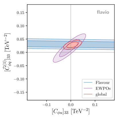
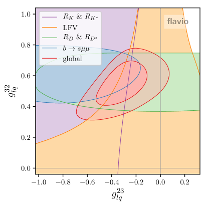
Figure 6: Left: Likelihood contours in the space of the two SMEFT Wilson coefficients that correspond to modified $Z$ couplings to left- or right-handed top quarks. The constraints from flavour physics (dominated by $B_{s}\to\mu^{+}\mu^{-}$) and EWPOs are complementary. Right: Likelihood contours in the plane of the couplings $g_{lq}^{23}$ and $g_{lq}^{32}$ of the $U_{1}$ vector leptoquark model at $1\sigma$ level.

4.7 Vector leptoquark solution to the $B$ anomalies

The $U_{1}$ vector leptoquark transforming as $(3,1)_{\frac{2}{3}}$ under the SM gauge group is the phenomenologically most successful single-multiplet scenario that simultaneously solves the charged- and neutral-current $B$ anomalies [84] as it does not give rise to $b\to s\nu\bar{\nu}$ at tree level [46] and is still allowed by direct searches [85].

Writing the leptoquark’s couplings to left-handed fermions as

$$\mathcal{L}_{U_{1}}\supset g_{lq}^{ji}\,\left(\bar{q}_{L}^{i}\gamma^{\mu}l_{L}^{j}\right)\,U_{\mu}+\text{h.c.}\,,$$ (16)

the solution of the neutral-current $B$ anomalies depends on the coupling combination $g_{lq}^{22}g_{lq}^{23*}$, while the charged-current anomalies require a sizable $g_{lq}^{32}g_{lq}^{33*}$.

Fig. 6 right shows the likelihood contours for the $U_{1}$ scenario in the plane $g_{lq}^{32}$ vs. $g_{lq}^{23}$ where we have fixed

$$m_{U_{1}} =2\,\text{TeV}\,, g_{lq}^{33} =1\,, g_{lq}^{22} =0.04^{2}\approx V_{cb}^{2}\,.$$ (17)

The LFV decays are important constraints to determine the allowed pattern of the couplings $g_{lq}^{ij}$ [87]. This can be seen from the orange contour in Fig. 6 right, which shows constraints from BR$(B\to K\tau^{+}\mu^{-})$, BR$(B\to K\mu^{+}\tau^{-})$, and BR$(\tau\to\phi\mu)$. The former two depend on the coupling combinations $g_{lq}^{33}g_{lq}^{22}$ and $g_{lq}^{23}g_{lq}^{32}$ respectively, whereas the latter is controlled by $g_{lq}^{32}g_{lq}^{22}$.

4.8 $B$ anomalies from third generation couplings

An interesting EFT scenario for the combined explanation of the $B$ anomalies in the neutral and charged currents is to assume TeV-scale NP in the purely third generation operators $[O_{lq}^{(1)}]_{3333}$ and $[O_{lq}^{(3)}]_{3333}$ in the interaction basis [88]. The effective Lagrangian in the Warsaw basis (as defined in WCxf [15]) can be written as

$$\mathcal{L}_{\text{eff}}\supset\frac{\lambda^{ij}_{\ell}\lambda^{kl}_{q}}{\Lambda^{2}}\left(C_{1}\bar{\ell}_{iL}\gamma_{\mu}\ell_{jL}\bar{q}_{kL}\gamma^{\mu}q_{lL}+C_{3}\bar{\ell}_{iL}\gamma_{\mu}\tau^{I}\ell_{jL}\bar{q}_{kL}\gamma^{\mu}\tau^{I}q_{lL}\right),$$ (18)

where $\lambda_{\ell}$ and $\lambda_{q}$ parameterize the mismatch between the interaction basis and the basis where the down-type quark mass matrix is diagonal.

As required by the data, purely third generation operators induce a large NP contribution in $b\to c\tau\bar{\nu}$, whereas in $b\to s\mu^{+}\mu^{-}$ comparatively smaller effects arise due to mixing on rotating to the mass basis.

In this context, ref. [89] found that electroweak corrections can lead to important effects in $Z$ pole observables and $\tau$ decays challenging this simultaneous solution for the $B$ anomalies. Since all the relevant observables as well as the SMEFT RG evolution are included in our global likelihood, we can reproduce these conclusions.

Figure 7: Likelihood contours at $2\sigma$ for various sets of observables for the scenario with mostly third generation couplings defined in eq. (18).

In figure 7 we show likelihood contours of the various observables in the plane of $C_{1}=C_{3}$ and $\lambda_{\ell}^{23}$. We have set $\Lambda=1$ TeV, $\lambda_{q}^{23}=-0.008$ and the relations $\lambda_{\ell,q}^{22}=(\lambda_{\ell,q}^{23})^{2}$, $\lambda_{\ell}^{33}=\lambda_{q}^{33}=1$ are imposed. Like [89], we find that the $2\sigma$ region for the precision $\tau$ decays does not overlap with the $2\sigma$ regions preferred by $R_{D^{(*)}}$ and $R_{K^{(*)}}$. Furthermore, the $2\sigma$ region from EWPOs has only a very small overlap with the $2\sigma$ region preferred by $R_{D^{(*)}}$. Compared to [89], we find a stronger constraint on the shift in the tau neutrino’s electroweak coupling. We have traced this difference back to the treatment of the LEP constraint in the invisible $Z$ width. [89] uses the invisible $Z$ width extracted by LEP [90], corresponding to the effective number of neutrino species $N_{\nu}=2.984\pm 0.008$, which favours a destructive interference with the SM at $2\sigma$. This number is obtained exclusively from $\sigma_{\text{had}}$, using the measured value of $R_{l}$ (assuming lepton flavour universality). Our treatment differs in two respects. First, since both $\sigma_{\text{had}}$ and $R_{e,\mu,\tau}$ are among the observables in the likelihood, we effectively use the SM values of $R_{e,\mu,\tau}$ rather than the measured ones when shifting only the neutrino coupling. This leads to a value $N_{\nu}=2.990\pm 0.007$, in better agreement with the SM value. Second, we include additional observables sensitive to the electroweak coupling of the tau neutrino, notably the total $Z$ width $\Gamma_{Z}$ and the $W\to\tau\nu$ branching ratio. Figure 8 shows the contributions of these three observables to the likelihood as well as their combination. While $\sigma_{\text{had}}$ alone favours a slightly shifted coupling (less significant than $2\sigma$ due to the different treatment of $R_{l}$), the combined constraints are in agreement with the SM at $1\sigma$ and more strongly disfavour a positive shift in $[C_{\phi l}^{(1)}]_{33}=-[C_{\phi l}^{(3)}]_{33}$.

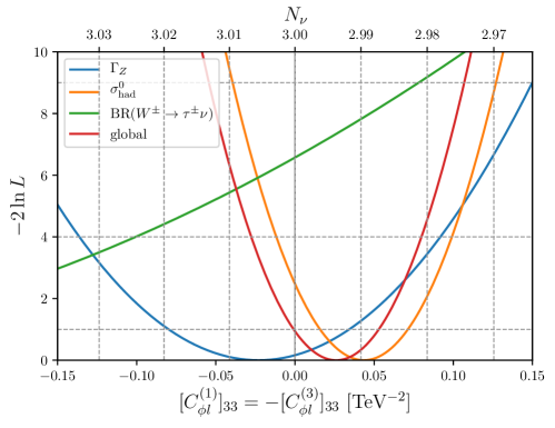
Figure 8: Contributions to the log-likelihood $\ln L$ from the observables sensitive to a shift in the tau neutrino’s electroweak coupling and their combination, relative to their respective extrema. The axis on top shows the effective number of neutrino species that would correspond to the relative modification of the $Z$ boson’s invisible width.

5 Usage

The global likelihood is accessed via the Python package smelli (SMEFT likelihood). Given a working installation of Python version 3.5 or above, the package can be installed with the simple command
⬇ 1python3 -m pip install smelli --user that downloads it from the Python package archive (PyPI) along with all required dependencies and installs it in the user’s home directory (no administrator privileges required). The source code of the package can be browsed via a public Github repository.

As with any Python package, smelli can be used as library imported from other scripts, directly in the command line interpreter, or in an interactive session. For interactive use, we recommend the Jupyter notebook that runs in a web browser. In all cases, the first step is to import the package and to initialize the class GlobalLikelihood,
⬇ 1import smelli 2gl = smelli.GlobalLikelihood() The initialization function takes two optional arguments:

• The argument eft (default value: 'SMEFT') can be set to 'WET' to obtain a likelihood in the parameter space of WET rather than SMEFT Wilson coefficients. In this case EWPOs are ignored.

• The argument basis allows to select a different WCxf basis (default: 'Warsaw' in the case of SMEFT, 'flavio' in the case of WET).

By default, smelli uses the leading logarithmic approximation for the SMEFT RG evolution, since it is faster than the full numerical solution of the coupled RGEs. This behaviour can be changed by setting the corresponding option of the wilson package after importing smelli, e.g.

⬇

1import smelli, wilson

2wilson.Wilson.set_default_option(’smeft_accuracy’, ’integrate’)

The next step is to select a point in Wilson coefficient space by using the parameter_point method. The Wilson coefficients must be provided in the EFT and basis fixed in the first step. There are three possible input formats:

• a Python dictionary (containing Wilson coefficient name/value pairs) and an input scale,

• as a WCxf data file in YAML or JSON format (specified by its file path as a string),

• as an instance of wilson.Wilson defined by the wilson package.

Using the first option, fixing the Wilson coefficient $[C_{lq}^{(1)}]_{2223}$ to $10^{-8}\,\text{GeV}^{-2}$ at the scale 1 TeV is achieved with

⬇

1glp = gl.parameter_point({’lq1_2223’: 1e-8}, scale=1000)

Note that, consistently with the WCxf format, all dimensionful values are expected to be in appropriate powers of GeV. The same result could be achieved with a WCxf file in YAML format,

⬇

1eft SMEFT

2basis Warsaw

3scale 1000

4values

5 lq1_2223 1e-8

that is imported as

⬇

1glp = gl.parameter_point(’my_wc.yaml’)

The variable glp defined above holds an instance of the GlobalLikelihoodPoint class that gives access to the results for the chosen parameter point. Its most important methods are

• glp.log_likelihood_global() returns the numerical value of the logarithm of the likelihood minus its SM value $\ln\Delta L$, i.e. the logarithm of the likelihood ratio or $-\Delta\chi^{2}/2$ when writing the likelihood as $L=e^{-\chi^{2}/2}$.

• glp.log_likelihood_dict() returns a dictionary with the contributions to $\ln\Delta L$ from the individual products in (3).

• glp.obstable() returns a pandas.DataFrame table-like object that lists all the individual observables with their experimental and theoretical central values and uncertainties ordered by their “pull” that is defined by $\sqrt{|\Delta\chi^{2}_{i}|}$ where $-\chi^{2}_{i}/2$ is their individual contribution to the log-likelihood neglecting all correlations. This table can be useful to get a better understanding of the likelihood value at a given point. However it should be used with caution. In particular, the log-likelihood is not equal to the sum of the individual contributions obtained from the pulls, as there can be significant correlations between them. Also, the uncertainties listed in this table can be inaccurate in the case of strongly non-Gaussian probability distributions.

The observables with the highest pulls in the SM as obtained by this method are shown for illustration in table 1. A few comments are in order.

• The largest deviation is in the branching ratio of $B_{s}\to\phi\mu^{+}\mu^{-}$ at low $q^{2}$, where the prediction relies strongly on the form factors from [91].

• The observable $R_{\tau\ell}(B\to D^{\ast}\ell^{+}\nu)$ is nothing but $R_{D^{\ast}}$, while $\langle R_{\mu e}\rangle(B^{\pm}\to K^{\pm}\ell^{+}\ell^{-})^{[1.0,6.0]}$ and $\langle R_{\mu e}\rangle(B^{0}\to K^{\ast 0}\ell^{+}\ell^{-})^{[a,b]}$ are $R_{K}$ and $R_{K^{\ast}}$, respectively. $\langle A_{\text{FB}}^{\ell h}\rangle(\Lambda_{b}\to\Lambda\mu^{+}\mu^{-})$ is denoted $K_{6}$ in [92]. We use the full observable names as defined in flavio here.

• The SM uncertainties in $\epsilon^{\prime}/\epsilon$ are entirely due to matrix elements from lattice QCD [54, 55].

Observable	Prediction	Measurement		Pull
$\langle\frac{d\overline{\text{BR}}}{dq^{2}}\rangle(B_{s}\to\phi\mu^{+}\mu^{-})^{[1.0,6.0]}$	$\left(5.39\pm 0.66\right)\times 10^{-8}\ \frac{1}{\text{GeV}^{2}}$	$\left(2.57\pm 0.37\right)\times 10^{-8}\ \frac{1}{\text{GeV}^{2}}$	[93, 94]	$3.7\sigma$
$a_{\mu}$	$\left(1.1659182\pm 0.0000004\right)\times 10^{-3}$	$\left(1.1659209\pm 0.0000006\right)\times 10^{-3}$	[95]	$3.4\sigma$
$\langle P_{5}^{\prime}\rangle(B^{0}\to K^{\ast 0}\mu^{+}\mu^{-})^{[4,6]}$	$-0.757\pm 0.074$	$-0.21\pm 0.15$	[96, 35]	$3.3\sigma$
$R_{\tau\ell}(B\to D^{\ast}\ell^{+}\nu)$	$0.255$	$0.306\pm 0.018$	[97, 48, 49, 98]	$2.9\sigma$
$\langle A_{\text{FB}}^{\ell h}\rangle(\Lambda_{b}\to\Lambda\mu^{+}\mu^{-})^{[15,20]}$	$0.1400\pm 0.0074$	$0.249\pm 0.040$	[92]	$2.7\sigma$
$\epsilon^{\prime}/\epsilon$	$\left(-0.3\pm 5.9\right)\times 10^{-4}$	$\left(1.66\pm 0.23\right)\times 10^{-3}$	[99]	$2.7\sigma$
$\langle R_{\mu e}\rangle(B^{\pm}\to K^{\pm}\ell^{+}\ell^{-})^{[1.0,6.0]}$	$1.001$	$0.745\pm 0.097$	[33]	$2.6\sigma$
$\text{BR}(W^{\pm}\to\tau^{\pm}\nu)$	$0.1084$	$0.1138\pm 0.0021$	[100]	$2.6\sigma$
$\langle R_{\mu e}\rangle(B^{0}\to K^{\ast 0}\ell^{+}\ell^{-})^{[1.1,6.0]}$	$1.00$	$0.68\pm 0.12$	[34]	$2.5\sigma$
$A_{\text{FB}}^{0,b}$	$10.31\times 10^{-2}$	$\left(9.92\pm 0.16\right)\times 10^{-2}$	[90]	$2.4\sigma$
$\langle R_{\mu e}\rangle(B^{0}\to K^{\ast 0}\ell^{+}\ell^{-})^{[0.045,1.1]}$	$0.93$	$0.65\pm 0.12$	[34]	$2.4\sigma$

Table 1: Observables with highest pulls in the SM.

6 Conclusions

In this paper we have presented a likelihood function in the space of dimension-6 Wilson coefficients of the SMEFT. This function is made publicly available in the form of the Python package smelli, building on the existing public codes flavio and wilson. At present, the likelihood includes numerous observables from $B$ and $K$ decays, EWPOs, neutral meson mixing, LFV and CP violating processes and many more, counting a total of 265 observables. We have demonstrated its validity and usefulness by reproducing various results given in the literature. In passing, we have also pointed out new results, in particular the fact that one of the two possible solutions to the $R_{D}$ and $R_{D^{*}}$ anomalies involving the tensor operator is excluded by the recent Belle measurement of the longitudinal polarization fraction in $B\to D^{*}\tau\nu$, which is included in our likelihood (see section 4.3).

Clearly, the 265 observables do not constrain the entire 2499-dimensional parameter space of SMEFT Wilson coefficients yet. Observables that are still missing include

• Higgs production and decay [101, 102, 64] including $h\to\gamma\gamma$ [103, 104, 105],

• top physics [106, 107, 108, 109],

• further low-energy observables [17], such as neutrino scattering, parity violation in atoms, and quark pair production in $e^{+}e^{-}$ collisions,

• non-leptonic $B$ decays [110],

• rare $D$ decays [111, 112, 113, 114],

• further hadronic tau decays [115, 116],

• beta decay [117, 18, 19],

• paramagnetic EDMs [118, 30],

among others. Furthermore, as discussed at the end of section 2, a major limitation of the nuisance-free likelihood we have constructed is that several classes of observables cannot be incorporated consistently without scanning over nuisance parameters. The next step in generalizing our results would be to allow the 4 parameters of the CKM matrix to vary in addition to the Wilson coefficients. This would make it possible to consistently include semi-leptonic charged-current $B$ and $K$ decays with general NP effects.

We hope that the groundwork laid by us will allow the community to build a more and more global likelihood as a powerful tool to constrain UV models from precision measurements.

Note added

After our preprint was published, ref. [119] appeared that proposes a procedure for a consistent treatment of the CKM matrix in the presence of dimension-6 contributions. Implemented in our framework, this would allow to include semi-leptonic charged-current decays without the need to scan over nuisance parameters.

Appendix A Conventions and caveats

In this appendix, we fix some of our conventions necessary for a consistent usage of the likelihood function and recall a few caveats when dealing with different bases of Wilson coefficients.

A.1 SMEFT flavour basis

Within SMEFT, a complete basis of gauge-invariant operators has to be chosen. Here we adopt the “Warsaw basis”, as defined in [2]. This basis is defined in the interaction basis above the electroweak scale. Having fixed this basis, there remains a continuous choice for the basis in flavour space, parameterized by the $U(3)^{5}$ flavour symmetry of unitary fermion field rotations. Anticipating spontaneous symmetry breaking at the EW scale motivates the choice of basis closely related to the mass eigenbasis. Due to the misalignment of the up- and down sector, a choice has to be made concerning the diagonality of the mass matrices. Above the electroweak scale, only five instead of the usual six fermion-field rotation matrices can be used to diagonalize the three mass matrices of the SM. This is because left-handed up- and down-type quarks form doublets of the unbroken $SU(2)_{L}$ symmetry and therefore have to be rotated by the same matrix. Denoting the quark rotations by

$$\psi\to U_{\psi}\psi\,,\hskip 28.45274pt\psi=q,u,d,$$ (19)

leads to the following quark masses including dimension-6 corrections [120]:

$$M_{u} =\frac{v}{\sqrt{2}}U_{q}^{{\dagger}}\left(Y_{u}-\frac{v^{2}}{2}C_{u\phi}\right)U_{u}\,,$$ (20)

$$M_{d} =\frac{v}{\sqrt{2}}U_{q}^{{\dagger}}\left(Y_{d}-\frac{v^{2}}{2}C_{d\phi}\right)U_{d}\,.$$ (21)

Choosing the up-type mass matrix to be diagonal results in the “Warsaw-up” basis, such defined in the Wilson coefficient exchange format (WCxf) [15]. This is equivalent of choosing $U_{q}=U_{u_{L}}=U_{d_{L}}V^{{\dagger}}$, where $U_{u_{L}},U_{d_{L}}$ are the rotation matrices of the left-handed up- and down-quarks, which diagonalize the corresponding mass matrices, and $V$ is the CKM matrix. Therefore, in the Warsaw-up basis, the mass matrices read:

$$M_{u} =\hat{M}_{u}\,,$$ (22)

$$M_{d} =V\hat{M}_{d}\,,$$ (23)

with the diagonal matrices $\hat{M}_{u},\hat{M}_{d}$.

Furthermore, all operators containing left-handed down-type quarks are rotated by $V$ compared to the usual Warsaw basis, after having absorbed factors of $U_{u_{L}}$ in the Wilson coefficients. For example the operator $O_{qe}^{ijkl}=(\bar{q}_{i}\gamma_{\mu}q_{j})(\bar{e}_{k}\gamma^{\mu}e_{l})$ in the Warsaw basis

$$C_{qe}^{ijkl}O_{qe}^{ijkl}=C_{qe}^{ijkl}(\bar{u}_{L}^{i}\gamma_{\mu}u_{L}^{j}+\bar{d}_{L}^{i}\gamma_{\mu}d_{L}^{j})(\bar{e}_{R}^{k}\gamma^{\mu}e_{R}^{l})\,,$$ (24)

will read after performing quark rotations and choosing the Warsaw-up basis (denoted by a hat):

$$C_{qe}^{ijkl}O_{qe}^{ijkl}\to \,C_{qe}^{ijkl}\left((U^{{\dagger}}_{u_{L}})_{ia}(U_{u_{L}})_{jb}\bar{u}_{L}^{a}\gamma_{\mu}u_{L}^{b}\,+(U^{{\dagger}}_{d_{L}})_{ia}(U_{d_{L}})_{jb}(\bar{d}_{L}^{a}\gamma_{\mu}d_{L}^{b})\right)(\bar{e}_{R}^{k}\gamma^{\mu}e_{R}^{l})$$ (25)

$$= \underbrace{C_{qe}^{ijkl}(U^{{\dagger}}_{d_{L}})_{ia}(U_{d_{L}})_{jb}}_{=:\,\widehat{C}_{qe}^{ijkl}}\underbrace{(\bar{u}_{L}^{a}\gamma_{\mu}u_{L}^{b}+(V^{{\dagger}})_{af}(V)_{bg}\bar{d}_{L}^{f}\gamma_{\mu}d_{L}^{g})(\bar{e}_{R}^{k}\gamma^{\mu}e_{R}^{l})}_{=:\,\widehat{O}_{qe}^{ijkl}}$$

$$= \,\widehat{C}_{qe}^{ijkl}\widehat{O}_{qe}^{ijkl}\,.$$

A.2 Non-redundant SMEFT basis

To derive the complete anomalous dimension matrix [8, 6, 7] as well as the complete tree-level matching [13] of the SMEFT onto WET it is convenient to allow for all possible flavour combinations in the SMEFT operators. Nevertheless, many operators are symmetric under the exchange of flavour indices. This is for example the case for four-fermi operators consisting of two identical fermion currents, like the operator $O_{dd}^{ijkl}$:

$$O_{dd}^{ijkl}=(\bar{d}^{i}_{R}\gamma_{\mu}d^{j}_{R})(\bar{d}^{k}_{R}\gamma^{\mu}d^{l}_{R})\,,$$ (26)

for which clearly

$$O_{dd}^{abcd}=O_{dd}^{cdab}\,.$$ (27)

For the computation of physical processes it can however be more convenient to choose a minimal basis, in which all operators are independent of each other. Such a choice avoids unwanted symmetry factors in the Lagrangian. For example the Lagrangian written in a redundant basis featuring the operator $O_{dd}$ would contain terms of the form

$$\mathcal{L}_{\text{red}}\supset \,C^{1122}_{dd}O^{1122}_{dd}+C^{2211}_{dd}O^{2211}_{dd}$$ (28)

$$= \,C^{1122}_{dd}O^{1122}_{dd}+C^{2211}_{dd}O^{1122}_{dd}$$

$$= \,\left(C^{1122}_{dd}+C^{2211}_{dd}\right)O^{1122}_{dd}$$

$$= \,2C^{1122}_{dd}O^{1122}_{dd}$$

$$= \,2C^{2211}_{dd}O^{2211}_{dd}\,,$$

whereas in a non-redundant basis only one flavour combination is taken into account:

$$\mathcal{L}\supset C^{1122}_{dd}O^{1122}_{dd}\,,$$ (29)

and the redundant contribution is not part of the Lagrangian.

Furthermore, such symmetry factors can also enter the beta functions of the Wilson coefficients, since contributions from operators that are not linearly independent are counted individually. For example the beta function of the Wilson coefficient $C_{dd}$ in a redundant SMEFT basis contains terms of the form [8]:

$$\dot{C}_{dd}^{prst}=\frac{2}{3}g_{1}^{2}N_{c}y_{d}^{2}(C_{dd}^{prww}+C_{dd}^{wwpr})\delta_{st}+\ldots\,\,\,.$$ (30)

Therefore, operators with symmetric index combinations, like f.e. $prst=aabb,\,a\neq b$, get the same contribution from $C_{dd}^{aaww}$ and $C_{dd}^{wwaa}$, whereas in a non-redundant basis, only one of such contributions is present. The operator corresponding to the second contribution is not included in the Lagrangian.

This issue has to be taken into account when using the results of [8, 6, 7, 11, 13] together with a non-redundant basis, like the one defined in [9]. All operators of the non-redundant basis exhibiting such symmetries have to be divided by their corresponding symmetry factor $S$ before the running and multiplied by $S$ after the running to cancel the effect of the redundant operators in the RGEs. Similar comments apply to the matching at the EW scale and the running below the EW scale.

Moreover, the choice of basis has to be made before making it minimal by discarding redundant operators, since a basis change can reintroduce redundant operators. Looking at the example of $O^{(1),prst}_{qq}$ in the Warsaw basis with diagonal up quark mass matrix (denoted with a hat) and diagonal down quark mass matrix (no hat), respectively, one finds for the index combination $prst=1122$ [10]:

$$\widehat{O}_{qq}^{(1),1122}=V_{ui}\,V^{*}_{uj}\,V_{ck}\,V^{*}_{cl}\,O_{qq}^{(1),ijkl}\,.$$ (31)

The operator $\widehat{O}_{qq}^{(1),1122}$ in the Warsaw-up basis therefore depends in particular on the operator $O_{qq}^{(1),1122}$ and its redundant counterpart $O_{qq}^{(1),2211}$.

We stress that, being based on WCxf, the input to our likelihood function always refers to the basis without any redundant operators.

A.3 Definitions

A frequently overlooked ambiguity is the sign convention for the covariant derivative, that affects the overall sign of all dipole and triple gauge boson operators in both SMEFT and WET (see e.g. [2]). For definiteness, we specify our conventions here:

$$D_{\mu}\psi =\partial_{\mu}+ieQ_{\psi}A_{\mu}+ig_{s}T^{A}G^{A}_{\mu}\,,$$ (32)

$$F_{\mu\nu} =\partial_{\mu}A_{\nu}-\partial_{\nu}A_{\mu}\,,$$ (33)

$$G_{\mu\nu}^{A} =\partial_{\mu}G_{\nu}^{A}-\partial_{\nu}G_{\mu}^{A}-g_{s}f^{ABC}G_{\mu}^{B}G_{\nu}^{C}\,,$$ (34)

$$\sigma_{\mu\nu} =\frac{i}{2}\left[\gamma_{\mu},\gamma_{\nu}\right]\,.$$ (35)

This sign convention for the covariant derivative is prevalent in the flavour physics literature and corresponds to the “usual” sign of the $b\to s\gamma$ dipole Wilson coefficient in the SM, but differs from several textbooks, see [121] for an overview. The convention for $\sigma_{\mu\nu}$ is also the most common one, but there are notable exceptions, e.g. [122].

With these conventions, one obtains the following relation between the effective Lagrangian in the WCxf flavio basis

$$\mathcal{L}\supset i\bar{\psi}\not{D}\psi+\left[C_{\gamma}^{\psi}~{}(\bar{\psi}\sigma_{\mu\nu}P_{R}\psi)~{}F^{\mu\nu}+C_{g}^{\psi}~{}(\bar{\psi}\sigma_{\mu\nu}T^{A}P_{R}\psi)~{}G^{A\,\mu\nu}+\text{h.c.}\right]$$ (36)

and the the anomalous magnetic moment of a fermion $\psi$ with electric charge $Q_{\psi}$,

$$a_{\psi}=-\frac{4m}{eQ_{\psi}}\,\text{Re}(C_{\gamma}^{\psi})\,.$$ (37)

Appendix B $\tau\to\ell V$ decays

In the following, we summarize the full tree-level results of the $\tau\to\ell V$ decay width $\Gamma_{\tau\to\ell V}$ in the WET, where $V\in\{\rho,\phi\}$ is a vector meson and $\ell\in\{e,\mu\}$ is a lepton. The decay width can be expressed in terms of the squared amplitude $\overline{|\mathcal{M}_{\tau\to\ell V}|}^{2}$, which has been averaged over initial spins and summed over final spins and polarizations. One finds (cf. [123])

$$\Gamma_{\tau\to\ell V}=\frac{\sqrt{\lambda(m_{\tau}^{2},m_{\ell}^{2},m_{V}^{2})}}{16\,\pi\,m_{\tau}^{3}}\,\overline{|\mathcal{M}_{\tau\to\ell V}|}^{2},$$ (38)

where

$$\lambda(a,b,c)=a^{2}+b^{2}+c^{2}-2(ab+ac+bc)$$ (39)

is the Källén function[124].

B.1 Squared amplitudes

The $\tau\to\ell V$ matrix element due to generic couplings of the vector meson to the leptonic vector current can be written as

$$\mathcal{M}^{\text{VC}}_{\tau\to\ell V}=\epsilon_{\mu}^{*}(p_{V})\,\bar{\ell}(p_{\ell})\,\gamma^{\mu}\left(g_{L}^{\tau\ell V}\,P_{L}+g_{R}^{\tau\ell V}\,P_{R}\right)\tau(p_{\tau}),$$ (40)

where $p_{\tau}$, $p_{\ell}$, and $p_{V}$ are the momenta of $\tau$, $\ell$, and $V$, respectively, and $g_{L}^{\tau\ell V}$ and $g_{R}^{\tau\ell V}$ are effective coupling constants. Squaring this matrix element, averaging over initial spins, and summing over final spins and polarizations yields

$$\overline{|\mathcal{M}^{\text{VC}}_{\tau\to\ell V}|}^{2}=\frac{1}{2}\Bigg{\{} \left(\left|g_{L}^{\tau\ell V}\right|^{2}+\left|g_{R}^{\tau\ell V}\right|^{2}\right)\left(\frac{\left(m_{\tau}^{2}-m_{\ell}^{2}\right)^{2}}{m_{V}^{2}}+m_{\tau}^{2}+m_{\ell}^{2}-2\,m_{V}^{2}\right)$$ (41)

$$-12\,m_{\tau}\,m_{\ell}\,\operatorname{Re}\Bigg{(}g_{R}^{\tau\ell V}\,\left(g_{L}^{\tau\ell V}\right)^{\!*}\Bigg{)}\Bigg{\}}.$$

The $\tau\to\ell V$ matrix element due to generic couplings of the vector meson to the leptonic tensor current can be written as

$$\mathcal{M}^{\text{TC}}_{\tau\to\ell V} =i\,p_{V}^{\alpha}\,\epsilon^{*\beta}(p_{V})\,$$ (42)

$$\times\bar{\ell}(p_{\ell})\,\sigma^{\mu\nu}\left(g_{\alpha\mu}\,g_{\beta\nu}\left(g_{TL}^{\tau\ell V}\,P_{L}+g_{TR}^{\tau\ell V}\,P_{R}\right)+\frac{i}{2}\,\epsilon_{\alpha\beta\mu\nu}\left(\tilde{g}_{TL}^{\tau\ell V}\,P_{L}+\tilde{g}_{TR}^{\tau\ell V}\,P_{R}\right)\right)\tau(p_{\tau}),$$

where $g_{TL}^{\tau\ell V}$, $g_{TR}^{\tau\ell V}$, $\tilde{g}_{TL}^{\tau\ell V}$, and $\tilde{g}_{TR}^{\tau\ell V}$ are effective coupling constants. Squaring this matrix element, averaging over initial spins, and summing over final spins and polarizations yields

$$\overline{|\mathcal{M}^{\text{TC}}_{\tau\to\ell V}|}^{2}=\frac{m_{V}^{2}}{2}\Bigg{\{} \left(\frac{2\left(m_{\tau}^{2}-m_{\ell}^{2}\right)^{2}}{m_{V}^{2}}-m_{\tau}^{2}-m_{\ell}^{2}-m_{V}^{2}\right)\left(\left|g_{TL}^{\tau\ell V}-\tilde{g}_{TL}^{\tau\ell V}\right|^{2}+\left|g_{TR}^{\tau\ell V}+\tilde{g}_{TR}^{\tau\ell V}\right|^{2}\right)$$ (43)

$$-12\,m_{\tau}\,m_{\ell}\,\operatorname{Re}\Bigg{(}\left(g_{TR}^{\tau\ell V}+\tilde{g}_{TR}^{\tau\ell V}\right)\left(g_{TL}^{\tau\ell V}-\tilde{g}_{TL}^{\tau\ell V}\right)^{\!\!*}\Bigg{)}\Bigg{\}}.$$

The full $\tau\to\ell V$ amplitude $\mathcal{M}^{\text{full}}_{\tau\to\ell V}$ is given by the sum of the vector current amplitude $\mathcal{M}^{\text{VC}}_{\tau\to\ell V}$ and the tensor current amplitude $\mathcal{M}^{\text{TC}}_{\tau\to\ell V}$,

$$\mathcal{M}^{\text{full}}_{\tau\to\ell V}=\mathcal{M}^{\text{VC}}_{\tau\to\ell V}+\mathcal{M}^{\text{TC}}_{\tau\to\ell V}.$$ (44)

Squaring the full amplitude, averaging over initial spins, and summing over final spins and polarizations yields

$$\overline{|\mathcal{M}^{\text{full}}_{\tau\to\ell V}|}^{2}=\overline{|\mathcal{M}^{\text{VC}}_{\tau\to\ell V}|}^{2}+\overline{|\mathcal{M}^{\text{TC}}_{\tau\to\ell V}|}^{2}+\mathcal{I},$$ (45)

where the interference term $\mathcal{I}$ is given by

$$\mathcal{I}= 3\,m_{\tau}\left(m_{\tau}^{2}-m_{\ell}^{2}-m_{V}^{2}\right)\!\!\!\!\!\! \operatorname{Re}\Bigg{(}g_{L}^{\tau\ell V}\left(g_{TR}^{\tau\ell V}+\tilde{g}_{TR}^{\tau\ell V}\right)^{*}+g_{R}^{\tau\ell V}\left(g_{TL}^{\tau\ell V}-\tilde{g}_{TL}^{\tau\ell V}\right)^{*}\Bigg{)}$$ (46)

$$+ 3\,m_{\ell}\left(m_{\ell}^{2}-m_{\tau}^{2}-m_{V}^{2}\right)\!\!\!\!\!\! \operatorname{Re}\Bigg{(}g_{R}^{\tau\ell V}\left(g_{TR}^{\tau\ell V}+\tilde{g}_{TR}^{\tau\ell V}\right)^{*}+g_{L}^{\tau\ell V}\left(g_{TL}^{\tau\ell V}-\tilde{g}_{TL}^{\tau\ell V}\right)^{*}\Bigg{)}.$$

B.2 Effective coupling constants in the WET

B.2.1 Vector operators

The semi-leptonic vector operators

$$\mathcal{L}_{\text{eff}}\subset\ \sum_{\ell\in\{e,\mu\},q\in\{u,d,s\}}\Big{\{} C_{VLL}^{\tau\ell qq} \!\!(\bar{\ell}_{L}\gamma^{\mu}\tau_{L})(\bar{q}_{L}\gamma_{\mu}q_{L})$$ (47)

$$+ C_{VLR}^{\tau\ell qq} \!\!(\bar{\ell}_{L}\gamma^{\mu}\tau_{L})(\bar{q}_{R}\gamma_{\mu}q_{R})$$

$$+ C_{VLR}^{qq\tau\ell} \!\!\vphantom{\Bigg{\{}}(\bar{\ell}_{R}\gamma^{\mu}\tau_{R})(\bar{q}_{L}\gamma_{\mu}q_{L})$$

$$+ C_{VRR}^{\tau\ell qq} \!\!(\bar{\ell}_{R}\gamma^{\mu}\tau_{R})(\bar{q}_{R}\gamma_{\mu}q_{R})\Big{\}}+\text{h.c.}$$

contribute to the vector current amplitude $\mathcal{M}^{\text{VC}}_{\tau\to\ell V}$. Using the vacuum to vector meson matrix element of the quark vector current for the case $V=\phi$ (cf. e.g. [125]),

$$\left<\phi|\bar{s}\gamma_{\mu}s|0\right>=m_{\phi}\,f_{\phi}\,\epsilon_{\mu}^{*},$$ (48)

where $f_{\phi}$ is the $\phi$ decay constant and $m_{\phi}$ the $\phi$ mass, the effective couplings $g_{L}^{\tau\ell\phi}$ and $g_{R}^{\tau\ell\phi}$ are given by

$$g_{L}^{\tau\ell\phi} =\frac{1}{2}\,m_{\phi}\,f_{\phi}\,\left(C_{VLL}^{\tau\ell ss}+C_{VLR}^{\tau\ell ss}\right),$$ (49)

$$g_{R}^{\tau\ell\phi} =\frac{1}{2}\,m_{\phi}\,f_{\phi}\,\left(C_{VRR}^{\tau\ell ss}+C_{VLR}^{ss\tau\ell}\right).$$

In the case $V=\rho$, the vacuum to vector meson matrix element is

$$\left<\rho\left|\frac{\bar{u}\gamma_{\mu}u-\bar{d}\gamma_{\mu}d}{\sqrt{2}}\right|0\right>=m_{\rho}\,f_{\rho}\,\epsilon_{\mu}^{*},$$ (50)

and the effective couplings $g_{L}^{\tau\ell\rho}$ and $g_{R}^{\tau\ell\rho}$ are given by

$$g_{L}^{\tau\ell\rho} =\frac{1}{2}\,m_{\rho}\,f_{\rho}\,\left(\frac{C_{VLL}^{\tau\ell uu}-C_{VLL}^{\tau\ell dd}}{\sqrt{2}}+\frac{C_{VLR}^{\tau\ell uu}-C_{VLR}^{\tau\ell dd}}{\sqrt{2}}\right),$$ (51)

$$g_{R}^{\tau\ell\rho} =\frac{1}{2}\,m_{\rho}\,f_{\rho}\,\left(\frac{C_{VRR}^{\tau\ell u}-C_{VRR}^{\tau\ell dd}}{\sqrt{2}}+\frac{C_{VLR}^{uu\tau\ell}-C_{VLR}^{dd\tau\ell}}{\sqrt{2}}\right),$$

where $f_{\rho}$ and $m_{\rho}$ are the $\rho$’s decay constant and mass.

B.2.2 Dipole and tensor operators

The leptonic dipole operators

$$\mathcal{L}_{\text{eff}}\subset\ \sum_{\ell\in\{e,\mu\}}\Big{\{} C_{\gamma}^{\tau\ell} \!\!\!\!(\bar{\ell}_{L}\sigma^{\mu\nu}\tau_{R})\,F_{\mu\nu}$$ (52)

$$+ C_{\gamma}^{\ell\tau} \!\!\!\!(\bar{\tau}_{L}\sigma^{\mu\nu}\ell_{R})\,F_{\mu\nu}\Big{\}}+\text{h.c.}\,,$$

as well as the semi-leptonic tensor operators

$$\mathcal{L}_{\text{eff}}\subset\ \sum_{\ell\in\{e,\mu\},q\in\{u,d,s\}}\Big{\{} C_{TRR}^{\tau\ell qq} \!\!\!\!(\bar{\ell}_{L}\sigma^{\mu\nu}\tau_{R})\,(\bar{q}_{L}\sigma_{\mu\nu}q_{R})$$ (53)

$$+ C_{TRR}^{\ell\tau qq} \!\!\!\!(\bar{\tau}_{L}\sigma^{\mu\nu}\ell_{R})\,(\bar{q}_{L}\sigma_{\mu\nu}q_{R})\Big{\}}+\text{h.c.}\,,$$

contribute to the tensor current amplitude $\mathcal{M}^{\text{TC}}_{\tau\to\ell V}$. Following [58], the vacuum to vector meson matrix element of the electromagnetic field strength tensor $F_{\mu\nu}$ can be written as

$$\left<V\left|F_{\mu\nu}\right|0\right> =\frac{i\,f_{V}\,K_{V}}{m_{V}}\left({p_{V}}_{\mu}\,\epsilon_{\nu}^{*}-{p_{V}}_{\nu}\,\epsilon_{\mu}^{*}\right),$$ (54)

where ${p_{V}}_{\mu}$ is the outgoing momentum of the vector meson and the constant $K_{V}$ depends on the fermion content of the meson $V$ and the electric charges $Q_{f}$ of its constituent fermions. For $V=\phi$ and $V=\rho$, one finds

$$K_{\phi}=-e\,Q_{s}=\frac{1}{3}\,e,\quad\quad K_{\rho}=-e\frac{Q_{u}-Q_{d}}{\sqrt{2}}=-\frac{1}{\sqrt{2}}\,e.$$ (55)

The vacuum to vector meson matrix element of the quark tensor current for the case $V=\phi$ is given by (cf. e.g. [125])

$$\left<\phi|\bar{s}\sigma_{\mu\nu}s|0\right>=i\,{f_{T}}_{\phi}(\mu)\left({p_{\phi}}_{\mu}\,\epsilon_{\nu}^{*}-{p_{\phi}}_{\nu}\,\epsilon_{\mu}^{*}\right),$$ (56)

where ${p_{\phi}}_{\mu}$ is the outgoing momentum of the $\phi$ and ${f_{T}}_{\phi}(\mu)$ is its transverse decay constant, which depends on the scale $\mu$ at which the corresponding operator is renormalized. For $\tau$ decays, we set $\mu=1.8\,\text{GeV}$ and define

$${f_{T}}_{V}^{\tau}={f_{T}}_{V}(1.8\,\text{GeV}),\quad V\in\{\phi,\rho\}.$$ (57)

The contributions from dipole and tensor Wilson coefficients to the coupling constants $g_{TL}^{\tau\ell\phi}$, $g_{TR}^{\tau\ell\phi}$, $\tilde{g}_{TL}^{\tau\ell\phi}$, and $\tilde{g}_{TR}^{\tau\ell\phi}$ are thus given by

$$g_{TL}^{\tau\ell\phi} ={f_{T}}_{\phi}^{\tau}\,{C_{TRR}^{\ell\tau ss}}^{*}+\frac{2\,f_{\phi}\,K_{\phi}}{m_{\phi}}{C_{\gamma}^{\ell\tau}}^{*}, \quad\quad\tilde{g}_{TL}^{\tau\ell\phi} =-{f_{T}}_{\phi}^{\tau}\,{C_{TRR}^{\ell\tau ss}}^{*},$$ (58)

$$g_{TR}^{\tau\ell\phi} ={f_{T}}_{\phi}^{\tau}\,C_{TRR}^{\tau\ell ss}+\frac{2\,f_{\phi}\,K_{\phi}}{m_{\phi}}C_{\gamma}^{\tau\ell}, \quad\quad\tilde{g}_{TR}^{\tau\ell\phi} ={f_{T}}_{\phi}^{\tau}\,C_{TRR}^{\tau\ell ss}.$$

In the case $V=\rho$, the vacuum to vector meson matrix element of the quark tensor current is

$$\left<\rho\left|\frac{\bar{u}\sigma_{\mu\nu}u-\bar{d}\sigma_{\mu\nu}d}{\sqrt{2}}\right|0\right>=i\,{f_{T}}_{\rho}(\mu)\left({p_{\rho}}_{\mu}\,\epsilon_{\nu}^{*}-{p_{\rho}}_{\nu}\,\epsilon_{\mu}^{*}\right),$$ (59)

where ${f_{T}}_{\rho}(\mu)$ is the $\rho$ transverse decay constant and ${p_{\rho}}_{\mu}$ is its outgoing momentum. The effective couplings $g_{TL}^{\tau\ell\rho}$, $g_{TR}^{\tau\ell\rho}$, $\tilde{g}_{TL}^{\tau\ell\rho}$, and $\tilde{g}_{TR}^{\tau\ell\rho}$ are thus given by

$$g_{TL}^{\tau\ell\rho} ={f_{T}}_{\rho}^{\tau}\,\frac{{C_{TRR}^{\ell\tau uu}}^{*}-{C_{TRR}^{\ell\tau dd}}^{*}}{\sqrt{2}}+\frac{2\,f_{\rho}\,K_{\rho}}{m_{\rho}}{C_{\gamma}^{\ell\tau}}^{*}, \quad\tilde{g}_{TL}^{\tau\ell\rho} =-{f_{T}}_{\rho}^{\tau}\,\frac{{C_{TRR}^{\ell\tau uu}}^{*}-{C_{TRR}^{\ell\tau dd}}^{*}}{\sqrt{2}},$$ (60)

$$g_{TR}^{\tau\ell\rho} ={f_{T}}_{\rho}^{\tau}\,\frac{C_{TRR}^{\tau\ell uu}-C_{TRR}^{\tau\ell dd}}{\sqrt{2}}+\frac{2\,f_{\rho}\,K_{\rho}}{m_{\rho}}C_{\gamma}^{\tau\ell}, \quad\tilde{g}_{TR}^{\tau\ell\rho} ={f_{T}}_{\rho}^{\tau}\,\frac{C_{TRR}^{\tau\ell uu}-C_{TRR}^{\tau\ell dd}}{\sqrt{2}}.$$

Appendix C $\tau\to P\ell$ decays

C.1 $\tau\to\ell\pi^{0}$: Effective coupling constants in the WET

The matrix elements in this case can be defined as[126]

$$\left<\pi^{0}|\bar{u}\gamma_{\mu}\gamma_{5}u|0\right>=\frac{if_{\pi}p_{\pi\mu}}{\sqrt{2}},\ \ \ \ \ \left<\pi^{0}|\bar{d}\gamma_{\mu}\gamma_{5}d|0\right>=-\frac{if_{\pi}p_{\pi\mu}}{\sqrt{2}},$$ (61)

$$\left<\pi^{0}|\bar{u}\gamma_{5}u|0\right>=\frac{if_{\pi}m_{\pi}^{2}}{\sqrt{2}(m_{u}+m_{d})},\ \ \ \ \ \left<\pi^{0}|\bar{d}\gamma_{5}d|0\right>=-\frac{if_{\pi}m_{\pi}^{2}}{\sqrt{2}(m_{u}+m_{d})}.$$ (62)

here $f_{\pi}=130.2$MeV. For the process $\tau\to\pi^{0}\ell$, the relevant part of the WET Lagrangian reads

$$\mathcal{L}_{eff} \supset C_{VLL}^{\tau\ell qq}(\bar{\ell}_{L}\gamma^{\mu}\tau_{L})(\bar{q}_{L}\gamma_{\mu}q_{L})+C_{VLR}^{\tau\ell qq}(\bar{\ell}_{L}\gamma^{\mu}\tau_{L})(\bar{q}_{R}\gamma_{\mu}q_{R})$$

$$+ C_{VLR}^{qq\tau\ell}(\bar{\ell}_{R}\gamma^{\mu}\tau_{R})(\bar{q}_{L}\gamma_{\mu}q_{L})+C_{VRR}^{\tau\ell qq}(\bar{\ell}_{R}\gamma^{\mu}\tau_{R})(\bar{q}_{R}\gamma_{\mu}q_{R})$$

$$+ C_{SRL}^{\tau\ell qq}(\bar{\ell}_{L}\tau_{R})(\bar{q}_{R}q_{L})+C_{SRR}^{\tau\ell qq}(\bar{\ell}_{L}\tau_{R})(\bar{q}_{L}q_{R})$$

$$+ C_{SRR}^{*\ell\tau qq}(\bar{\ell}_{R}\tau_{L})(\bar{q}_{R}q_{L})+C_{SRL}^{*\ell\tau qq}(\bar{\ell}_{R}\tau_{L})(\bar{q}_{L}q_{R})+\text{h.c.}\ .$$

From $\mathcal{L}_{eff}$ using eqs. (61) and (62) and the momentum conservation, $p_{\pi}^{\mu}=p_{\tau}^{\mu}-p_{\ell}^{\mu}$, we can define the matrix element as

$${\mathcal{M}}_{\tau\ell\pi^{0}} = i(g_{L}^{\tau\ell\pi^{0}}\bar{\ell}P_{L}\tau+g_{R}^{\tau\ell\pi^{0}}\bar{\ell}P_{R}\tau)\,.$$ (64)

Here the couplings $g_{L}^{\tau\ell\pi^{0}}$ and $g_{R}^{\tau\ell\pi^{0}}$ are given by

$$g_{L}^{\tau\ell\pi^{0}}=s_{L}^{\tau\ell\pi^{0}}+(-v_{L}^{\tau\ell\pi^{0}}m_{l}+v_{R}^{\tau\ell\pi^{0}}m_{\tau}),\ \ g_{R}^{\tau\ell\pi^{0}}=s_{R}^{\tau\ell\pi^{0}}+(-v_{R}^{\tau\ell\pi^{0}}m_{l}+v_{L}^{\tau\ell\pi^{0}}m_{\tau}).$$ (65)

with the vector $v_{L}^{\tau\ell\pi^{0}}$, $v_{R}^{\tau\ell\pi^{0}}$ and scalar $s_{L}^{\tau\ell\pi^{0}}$, $s_{R}^{\tau\ell\pi^{0}}$ couplings

$$v_{L}^{\tau\ell\pi^{0}} = \frac{f_{\pi}}{\sqrt{2}}\left(\frac{C_{VLR}^{\tau\ell uu}-C_{VLL}^{\tau\ell uu}}{2}-\frac{C_{VLR}^{\tau\ell dd}-C_{VLL}^{\tau\ell dd}}{2}\right),$$ (66)

$$v_{R}^{\tau\ell\pi^{0}} = \frac{f_{\pi}}{\sqrt{2}}\left(\frac{C_{VRR}^{\tau\ell uu}-C_{VLR}^{uu\tau\ell}}{2}-\frac{C_{VRR}^{\tau\ell dd}-C_{VLR}^{dd\tau\ell}}{2}\right),$$ (67)

$$s_{R}^{\tau\ell\pi^{0}} = \frac{f_{\pi}m_{\pi}^{2}}{\sqrt{2}(m_{u}+m_{d})}\left(\frac{C_{SRR}^{\tau\ell uu}-C_{SRL}^{\tau\ell uu}}{2}-\frac{C_{SRR}^{\tau\ell dd}-C_{SRL}^{\tau\ell dd}}{2}\right),$$ (68)

$$s_{L}^{\tau\ell\pi^{0}} = \frac{f_{\pi}m_{\pi}^{2}}{\sqrt{2}(m_{u}+m_{d})}\left(\frac{C_{SRL}^{*\ell\tau uu}-C_{SRR}^{*\ell\tau uu}}{2}-\frac{C_{SRL}^{*\ell\tau dd}-C_{SRR}^{*\ell\tau dd}}{2}\right).$$ (69)

C.2 $\tau\to\ell K^{0}$: Effective coupling constants in the WET

For $K^{0}$ the pseudo vector matrix element is defined as[127]

$$\left<K^{0}(p)|\bar{d}\gamma_{\mu}\gamma_{5}s|0\right>=-if_{K}p_{K\mu},$$ (70)

and for the scalar current

$$\left<K^{0}(p)|\bar{d}\gamma_{5}s|0\right>=-\frac{if_{K}m_{K}^{2}}{m_{d}+m_{s}}.$$ (71)

The relevant part of the WET Lagrangian reads

$$\mathcal{L}_{eff} \supset K_{v}C_{9}^{sd\tau\ell}(\bar{d}_{L}\gamma_{\mu}s_{L})(\bar{\ell}\gamma^{\mu}\tau)+K_{v}C_{10}^{sd\tau\ell}(\bar{d}_{L}\gamma_{\mu}s_{L})(\bar{\ell}\gamma^{\mu}\gamma_{5}\tau)$$

$$+ K_{v}C_{9}^{{}^{\prime}sd\tau\ell}(\bar{d}_{R}\gamma_{\mu}s_{R})(\bar{\ell}\gamma^{\mu}\tau)+K_{v}C_{10}^{{}^{\prime}sd\tau\ell}(\bar{d}_{R}\gamma_{\mu}s_{R})(\bar{\ell}\gamma^{\mu}\gamma_{5}\tau)$$

$$+ K_{s}C_{S}^{sd\tau\ell}(\bar{d}_{L}s_{R})(\bar{\ell}\tau)+K_{s}C_{S}^{{}^{\prime}sd\tau\ell}(\bar{d}_{R}s_{L})(\bar{\ell}\tau)$$

$$+ K_{s}C_{P}^{sd\tau\ell}(\bar{d}_{L}s_{R})(\bar{\ell}\gamma_{5}\tau)+K_{s}C_{P}^{{}^{\prime}sd\tau\ell}(\bar{d}_{R}s_{L})(\bar{\ell}\gamma_{5}\tau),$$

here $K_{v}=\frac{4G_{F}}{\sqrt{2}}V_{ts}V_{td}^{*}\frac{e^{2}}{16\pi^{2}}$ and $K_{s}=m_{s}K_{v}$. The matrix element is given by

$$\mathcal{M}_{\tau\ell K^{0}} = ip_{K\mu}\left(g_{V}^{\tau\ell K^{0}}\bar{\ell}\gamma^{\mu}\tau+g_{A}^{\tau\ell K^{0}}\bar{\ell}\gamma^{\mu}\gamma_{5}\tau\right)+i\left(g_{S}^{\tau\ell K^{0}}\bar{\ell}\tau+g_{P}^{\tau\ell K^{0}}\bar{\ell}\gamma_{5}\tau\right),$$ (73)

with

$$g_{V}^{\tau\ell K^{0}} = \frac{-f_{K}K_{v}(-C_{9}^{sd\tau\ell}+C_{9}^{{}^{\prime}sd\tau\ell})}{2},\ \ \ \ g_{A}^{\tau\ell K^{0}}=\frac{-f_{K}K_{v}(-C_{10}^{sd\tau\ell}+C_{10}^{{}^{\prime}sd\tau\ell})}{2},$$ (74)

$$g_{S}^{\tau\ell K^{0}} = \frac{-K_{s}f_{K}m_{K}^{2}(C_{S}^{sd\tau\ell}-C_{S}^{{}^{\prime}sd\tau\ell})}{2(m_{s}+m_{d})},\ \ \ \ g_{P}^{\tau\ell K^{0}}=\frac{-K_{s}f_{K}m_{K}^{2}(C_{P}^{sd\tau\ell}-C_{P}^{{}^{\prime}sd\tau\ell})}{2(m_{s}+m_{d})}.$$ (75)

Using the momentum conservation, $p_{K}^{\mu}=p_{\tau}^{\mu}-p_{\ell}^{\mu}$, in Eq. 73, we can redefine the matrix element as

$${\mathcal{M}}_{\tau\ell K^{0}}=i\left(g_{L}^{\tau\ell K^{0}}\bar{\ell}P_{L}\tau+g_{R}^{\tau\ell K^{0}}\bar{\ell}P_{R}\tau\right)$$ (76)

here

$$g_{L}^{\tau\ell K^{0}}=\left(g_{VS}^{\tau\ell K^{0}}-g_{AP}^{\tau\ell K^{0}}\right)\ \ \ \ g_{R}^{\tau\ell K^{0}}=\left(g_{VS}^{\tau\ell K^{0}}+g_{AP}^{\tau\ell K^{0}}\right)$$ (77)

and the couplings $g_{VS}^{\tau\ell K^{0}}$ and $g_{AP}^{\tau\ell K^{0}}$ are given by

$$g_{VS}^{\tau\ell K^{0}}=g_{S}^{\tau\ell K^{0}}+g_{V}^{\tau\ell K^{0}}\left(m_{\tau}-m_{l}\right),\ \ g_{AP}^{\tau\ell K^{0}}=g_{P}^{\tau\ell K^{0}}-g_{A}^{\tau\ell K^{0}}\left(m_{l}+m_{\tau}\right).$$ (78)

C.3 Squared amplitude

The squared matrix element, summed over the final states and averaged over the initial states, is given by

$$|{\mathcal{M}}_{\tau\ell P}|^{2}= \frac{1}{2}\left(|g_{L}^{\tau\ell P}|^{2}+|g_{R}^{\tau\ell P}|^{2}\right)\left(m_{\tau}^{2}+m_{l}^{2}-m_{P}^{2}\right)$$ (79)

$$+2m_{l}m_{\tau}\left(\operatorname{Im}(g_{L}^{\tau\ell P})\operatorname{Im}(g_{R}^{\tau\ell P})+\operatorname{Re}(g_{L}^{\tau\ell P})\operatorname{Re}(g_{R}^{\tau\ell P})\right).$$

Appendix D List of observables

In this appendix we collect the SM predictions, uncertainties, experimental measurements (combinations in case of multiple measurements) and uncertainties for each individual observable. This table roughly corresponds to the output of the GlobalLikelihoodPoint.obstable method. It is only approximate in several cases, e.g. in case of non-Gaussian uncertainties present in the code. The “pull” ignores any correlations with other observables and is just meant as an indication of the agreement of an individual measurement with the SM. For observables where we neglect theory uncertainties, the predictions are just given as numbers. In the case of upper limits, we give the 95% confidence level limits in all cases.

Observable	Prediction	Measurement		Pull
$\langle A_{\text{FB}}\rangle(B^{0}\to K^{\ast 0}\mu^{+}\mu^{-})^{[0,2]}$	$-0.104\pm 0.011$	$0.07\pm 0.31$	[94]	$0.6\sigma$
$\langle A_{\text{FB}}\rangle(B^{0}\to K^{\ast 0}\mu^{+}\mu^{-})^{[2,4.3]}$	$\left(-2.6\pm 3.1\right)\times 10^{-2}$	$-0.11\pm 0.12$	[94, 128]	$0.7\sigma$
$\langle A_{\text{FB}}\rangle(B^{0}\to K^{\ast 0}\mu^{+}\mu^{-})^{[1,2]}$	$-0.156\pm 0.031$	$-0.28\pm 0.17$	[128]	$0.7\sigma$
$\langle A_{\text{FB}}\rangle(B^{0}\to K^{\ast 0}\mu^{+}\mu^{-})^{[4.3,6]}$	$0.133\pm 0.042$	$0.01\pm 0.15$	[128]	$0.8\sigma$
$\langle A_{\text{FB}}^{h}\rangle(\Lambda_{b}\to\Lambda\mu^{+}\mu^{-})^{[15,20]}$	$-0.272\pm 0.011$	$-0.299\pm 0.053$	[92]	$0.5\sigma$
$\langle A_{\text{FB}}^{\ell}\rangle(\Lambda_{b}\to\Lambda\mu^{+}\mu^{-})^{[15,20]}$	$-0.353\pm 0.021$	$-0.390\pm 0.041$	[92]	$0.8\sigma$
$\langle A_{\text{FB}}^{\ell h}\rangle(\Lambda_{b}\to\Lambda\mu^{+}\mu^{-})^{[15,20]}$	$0.1400\pm 0.0074$	$0.249\pm 0.040$	[92]	$2.7\sigma$
$\langle A_{T}^{\text{Im}}\rangle(B^{0}\to K^{\ast 0}e^{+}e^{-})^{[0.002,1.12]}$	$\left(3.2\pm 6.4\right)\times 10^{-4}$	$0.14\pm 0.23$	[129]	$0.6\sigma$
$\langle\text{BR}\rangle(B\to X_{s}e^{+}e^{-})^{[1.0,6.0]}$	$\left(1.74\pm 0.18\right)\times 10^{-6}$	$\left(2.01\pm 0.53\right)\times 10^{-6}$	[130]	$0.5\sigma$
$\langle\text{BR}\rangle(B\to X_{s}e^{+}e^{-})^{[14.2,25.0]}$	$\left(3.01\pm 0.34\right)\times 10^{-7}$	$\left(5.7\pm 1.9\right)\times 10^{-7}$	[130]	$1.4\sigma$
$\langle\text{BR}\rangle(B\to X_{s}\mu^{+}\mu^{-})^{[1.0,6.0]}$	$\left(1.67\pm 0.17\right)\times 10^{-6}$	$\left(7.5\pm 8.2\right)\times 10^{-7}$	[130]	$1.1\sigma$
$\langle\text{BR}\rangle(B\to X_{s}\mu^{+}\mu^{-})^{[14.2,25.0]}$	$\left(3.46\pm 0.39\right)\times 10^{-7}$	$\left(6.3\pm 3.0\right)\times 10^{-7}$	[130]	$0.9\sigma$
$\langle F_{L}\rangle(B^{0}\to K^{\ast 0}\mu^{+}\mu^{-})^{[0.04,2]}$	$0.388\pm 0.059$	$0.44\pm 0.11$	[96]	$0.4\sigma$
$\langle F_{L}\rangle(B^{0}\to K^{\ast 0}\mu^{+}\mu^{-})^{[2,4]}$	$0.799\pm 0.036$	$0.64\pm 0.12$	[96]	$1.3\sigma$
$\langle F_{L}\rangle(B^{0}\to K^{\ast 0}\mu^{+}\mu^{-})^{[4,6]}$	$0.711\pm 0.049$	$0.596\pm 0.053$	[96, 35]	$1.6\sigma$
$\langle F_{L}\rangle(B^{0}\to K^{\ast 0}\mu^{+}\mu^{-})^{[0,2]}$	$0.388\pm 0.059$	$0.27\pm 0.14$	[94]	$0.8\sigma$
$\langle F_{L}\rangle(B^{0}\to K^{\ast 0}\mu^{+}\mu^{-})^{[2,4.3]}$	$0.793\pm 0.036$	$0.758\pm 0.080$	[94, 128]	$0.4\sigma$
$\langle F_{L}\rangle(B^{0}\to K^{\ast 0}\mu^{+}\mu^{-})^{[1,2]}$	$0.725\pm 0.050$	$0.63\pm 0.10$	[128]	$0.8\sigma$
$\langle F_{L}\rangle(B^{0}\to K^{\ast 0}\mu^{+}\mu^{-})^{[4.3,6]}$	$0.703\pm 0.050$	$0.63\pm 0.12$	[128]	$0.6\sigma$
$\langle F_{L}\rangle(B^{0}\to K^{\ast 0}\mu^{+}\mu^{-})^{[1.1,2.5]}$	$0.760\pm 0.045$	$0.660\pm 0.083$	[35]	$1.1\sigma$
$\langle F_{L}\rangle(B^{0}\to K^{\ast 0}\mu^{+}\mu^{-})^{[2.5,4]}$	$0.796\pm 0.036$	$0.87\pm 0.10$	[35]	$0.7\sigma$
$\langle F_{L}\rangle(B^{0}\to K^{\ast 0}\mu^{+}\mu^{-})^{[15,19]}$	$0.340\pm 0.022$	$0.345\pm 0.030$	[35]	$0.1\sigma$
$\langle\overline{F_{L}}\rangle(B_{s}\to\phi\mu^{+}\mu^{-})^{[2.0,5.0]}$	$0.811\pm 0.019$	$0.68\pm 0.15$	[93]	$0.9\sigma$
$\langle\overline{F_{L}}\rangle(B_{s}\to\phi\mu^{+}\mu^{-})^{[15.0,19.0]}$	$0.341\pm 0.015$	$0.288\pm 0.068$	[93]	$0.8\sigma$
$\langle P_{1}\rangle(B^{0}\to K^{\ast 0}e^{+}e^{-})^{[0.002,1.12]}$	$\left(3.6\pm 2.3\right)\times 10^{-2}$	$-0.24\pm 0.24$	[129]	$1.2\sigma$
$\langle P_{1}\rangle(B^{0}\to K^{\ast 0}\mu^{+}\mu^{-})^{[0.04,2]}$	$\left(4.3\pm 2.9\right)\times 10^{-2}$	$-0.06\pm 0.31$	[96]	$0.3\sigma$
$\langle P_{1}\rangle(B^{0}\to K^{\ast 0}\mu^{+}\mu^{-})^{[2,4]}$	$\left(-9.5\pm 3.8\right)\times 10^{-2}$	$-0.78\pm 0.65$	[96]	$1.1\sigma$
$\langle P_{1}\rangle(B^{0}\to K^{\ast 0}\mu^{+}\mu^{-})^{[4,6]}$	$-0.178\pm 0.048$	$0.12\pm 0.30$	[96, 35]	$1.0\sigma$
$\langle P_{1}\rangle(B^{0}\to K^{\ast 0}\mu^{+}\mu^{-})^{[1,2]}$	$\left(4.4\pm 4.8\right)\times 10^{-2}$	$0.12\pm 0.47$	[131]	$0.2\sigma$
$\langle P_{1}\rangle(B^{0}\to K^{\ast 0}\mu^{+}\mu^{-})^{[2,4.3]}$	$-0.106\pm 0.038$	$-0.44\pm 0.45$	[131]	$0.7\sigma$
$\langle P_{1}\rangle(B^{0}\to K^{\ast 0}\mu^{+}\mu^{-})^{[4.3,6]}$	$-0.180\pm 0.049$	$0.45\pm 0.34$	[131]	$1.8\sigma$
$\langle P_{1}\rangle(B^{0}\to K^{\ast 0}\mu^{+}\mu^{-})^{[1.1,2.5]}$	$\left(2.3\pm 4.7\right)\times 10^{-2}$	$-0.45\pm 0.58$	[35]	$0.8\sigma$
$\langle P_{1}\rangle(B^{0}\to K^{\ast 0}\mu^{+}\mu^{-})^{[2.5,4]}$	$-0.116\pm 0.039$	$0.6\pm 2.0$	[35]	$0.4\sigma$
$\langle P_{1}\rangle(B^{0}\to K^{\ast 0}\mu^{+}\mu^{-})^{[15,19]}$	$-0.623\pm 0.043$	$-0.50\pm 0.10$	[35]	$1.1\sigma$
$\langle P_{2}\rangle(B^{0}\to K^{\ast 0}\mu^{+}\mu^{-})^{[1.1,2.5]}$	$-0.451\pm 0.014$	$-0.38\pm 0.17$	[35]	$0.4\sigma$
$\langle P_{2}\rangle(B^{0}\to K^{\ast 0}\mu^{+}\mu^{-})^{[2.5,4]}$	$-0.06\pm 0.10$	$-0.63\pm 0.87$	[35]	$0.6\sigma$
$\langle P_{2}\rangle(B^{0}\to K^{\ast 0}\mu^{+}\mu^{-})^{[4,6]}$	$0.292\pm 0.074$	$\left(3.2\pm 8.8\right)\times 10^{-2}$	[35]	$2.3\sigma$
$\langle P_{2}\rangle(B^{0}\to K^{\ast 0}\mu^{+}\mu^{-})^{[15,19]}$	$0.373\pm 0.017$	$0.361\pm 0.027$	[35]	$0.4\sigma$
$\langle P_{4}^{\prime}\rangle(B^{0}\to K^{\ast 0}\mu^{+}\mu^{-})^{[0.04,2]}$	$0.150\pm 0.018$	$0.36\pm 0.57$	[96]	$0.4\sigma$
$\langle P_{4}^{\prime}\rangle(B^{0}\to K^{\ast 0}\mu^{+}\mu^{-})^{[2,4]}$	$-0.349\pm 0.049$	$-0.98\pm 0.46$	[96]	$1.4\sigma$
$\langle P_{4}^{\prime}\rangle(B^{0}\to K^{\ast 0}\mu^{+}\mu^{-})^{[4,6]}$	$-0.504\pm 0.027$	$-0.30\pm 0.16$	[96, 35]	$1.2\sigma$
$\langle P_{4}^{\prime}\rangle(B^{0}\to K^{\ast 0}\mu^{+}\mu^{-})^{[1.1,2.5]}$	$\left(-6.4\pm 4.4\right)\times 10^{-2}$	$-0.17\pm 0.24$	[35]	$0.4\sigma$

Table 2: Quark flavour observables where theory uncertainties are taken into account (part 1/3).

Observable	Prediction	Measurement		Pull
$\langle P_{4}^{\prime}\rangle(B^{0}\to K^{\ast 0}\mu^{+}\mu^{-})^{[2.5,4]}$	$-0.393\pm 0.046$	$-0.72\pm 0.74$	[35]	$0.4\sigma$
$\langle P_{4}^{\prime}\rangle(B^{0}\to K^{\ast 0}\mu^{+}\mu^{-})^{[15,19]}$	$-0.6351\pm 0.0088$	$-0.598\pm 0.084$	[35]	$0.4\sigma$
$\langle P_{5}^{\prime}\rangle(B^{0}\to K^{\ast 0}\mu^{+}\mu^{-})^{[0.04,2]}$	$0.513\pm 0.036$	$0.67\pm 0.30$	[96]	$0.5\sigma$
$\langle P_{5}^{\prime}\rangle(B^{0}\to K^{\ast 0}\mu^{+}\mu^{-})^{[2,4]}$	$-0.41\pm 0.11$	$-0.33\pm 0.33$	[96]	$0.2\sigma$
$\langle P_{5}^{\prime}\rangle(B^{0}\to K^{\ast 0}\mu^{+}\mu^{-})^{[4,6]}$	$-0.757\pm 0.074$	$-0.21\pm 0.15$	[96, 35]	$3.3\sigma$
$\langle P_{5}^{\prime}\rangle(B^{0}\to K^{\ast 0}\mu^{+}\mu^{-})^{[1,2]}$	$0.288\pm 0.068$	$0.11\pm 0.34$	[131]	$0.5\sigma$
$\langle P_{5}^{\prime}\rangle(B^{0}\to K^{\ast 0}\mu^{+}\mu^{-})^{[2,4.3]}$	$-0.45\pm 0.10$	$-0.54\pm 0.36$	[131]	$0.2\sigma$
$\langle P_{5}^{\prime}\rangle(B^{0}\to K^{\ast 0}\mu^{+}\mu^{-})^{[4.3,6]}$	$-0.769\pm 0.072$	$-0.96\pm 0.26$	[131]	$0.7\sigma$
$\langle P_{5}^{\prime}\rangle(B^{0}\to K^{\ast 0}\mu^{+}\mu^{-})^{[1.1,2.5]}$	$0.139\pm 0.084$	$0.29\pm 0.21$	[35]	$0.7\sigma$
$\langle P_{5}^{\prime}\rangle(B^{0}\to K^{\ast 0}\mu^{+}\mu^{-})^{[2.5,4]}$	$-0.50\pm 0.10$	$-0.07\pm 0.35$	[35]	$1.2\sigma$
$\langle P_{5}^{\prime}\rangle(B^{0}\to K^{\ast 0}\mu^{+}\mu^{-})^{[15,19]}$	$-0.594\pm 0.035$	$-0.684\pm 0.082$	[35]	$1.0\sigma$
$\langle\overline{S_{3}}\rangle(B_{s}\to\phi\mu^{+}\mu^{-})^{[2.0,5.0]}$	$\left(-8.7\pm 3.9\right)\times 10^{-3}$	$-0.06\pm 0.21$	[93]	$0.3\sigma$
$\langle\overline{S_{3}}\rangle(B_{s}\to\phi\mu^{+}\mu^{-})^{[15.0,19.0]}$	$-0.2098\pm 0.0067$	$-0.09\pm 0.12$	[93]	$1.0\sigma$
$\langle\overline{S_{4}}\rangle(B_{s}\to\phi\mu^{+}\mu^{-})^{[2.0,5.0]}$	$-0.148\pm 0.018$	$-0.46\pm 0.36$	[93]	$0.9\sigma$
$\langle\overline{S_{4}}\rangle(B_{s}\to\phi\mu^{+}\mu^{-})^{[15.0,19.0]}$	$-0.3017\pm 0.0044$	$-0.14\pm 0.11$	[93]	$1.4\sigma$
$\langle\frac{d\text{BR}}{dq^{2}}\rangle(B^{+}\to K^{\ast+}\mu^{+}\mu^{-})^{[2.0,4.0]}$	$\left(4.87\pm 0.74\right)\times 10^{-8}\ \frac{1}{\text{GeV}^{2}}$	$\left(5.6\pm 1.6\right)\times 10^{-8}\ \frac{1}{\text{GeV}^{2}}$	[132]	$0.5\sigma$
$\langle\frac{d\text{BR}}{dq^{2}}\rangle(B^{+}\to K^{\ast+}\mu^{+}\mu^{-})^{[4.0,6.0]}$	$\left(5.43\pm 0.82\right)\times 10^{-8}\ \frac{1}{\text{GeV}^{2}}$	$\left(2.6\pm 1.0\right)\times 10^{-8}\ \frac{1}{\text{GeV}^{2}}$	[132]	$2.1\sigma$
$\langle\frac{d\text{BR}}{dq^{2}}\rangle(B^{+}\to K^{\ast+}\mu^{+}\mu^{-})^{[15.0,19.0]}$	$\left(6.44\pm 0.68\right)\times 10^{-8}\ \frac{1}{\text{GeV}^{2}}$	$\left(4.01\pm 0.83\right)\times 10^{-8}\ \frac{1}{\text{GeV}^{2}}$	[132]	$2.3\sigma$
$\langle\frac{d\text{BR}}{dq^{2}}\rangle(B^{+}\to K^{\ast+}\mu^{+}\mu^{-})^{[0,2]}$	$\left(8.7\pm 1.2\right)\times 10^{-8}\ \frac{1}{\text{GeV}^{2}}$	$\left(7.3\pm 4.8\right)\times 10^{-8}\ \frac{1}{\text{GeV}^{2}}$	[94]	$0.3\sigma$
$\langle\frac{d\text{BR}}{dq^{2}}\rangle(B^{+}\to K^{\ast+}\mu^{+}\mu^{-})^{[2,4.3]}$	$\left(4.90\pm 0.74\right)\times 10^{-8}\ \frac{1}{\text{GeV}^{2}}$	$\left(5.0\pm 3.7\right)\times 10^{-8}\ \frac{1}{\text{GeV}^{2}}$	[94]	$0.0\sigma$
$\langle\frac{d\text{BR}}{dq^{2}}\rangle(B^{\pm}\to K^{\pm}\mu^{+}\mu^{-})^{[1.1,2.0]}$	$\left(3.53\pm 0.62\right)\times 10^{-8}\ \frac{1}{\text{GeV}^{2}}$	$\left(2.33\pm 0.19\right)\times 10^{-8}\ \frac{1}{\text{GeV}^{2}}$	[132]	$1.8\sigma$
$\langle\frac{d\text{BR}}{dq^{2}}\rangle(B^{\pm}\to K^{\pm}\mu^{+}\mu^{-})^{[2.0,3.0]}$	$\left(3.51\pm 0.61\right)\times 10^{-8}\ \frac{1}{\text{GeV}^{2}}$	$\left(2.82\pm 0.21\right)\times 10^{-8}\ \frac{1}{\text{GeV}^{2}}$	[132]	$1.1\sigma$
$\langle\frac{d\text{BR}}{dq^{2}}\rangle(B^{\pm}\to K^{\pm}\mu^{+}\mu^{-})^{[3.0,4.0]}$	$\left(3.50\pm 0.60\right)\times 10^{-8}\ \frac{1}{\text{GeV}^{2}}$	$\left(2.54\pm 0.20\right)\times 10^{-8}\ \frac{1}{\text{GeV}^{2}}$	[132]	$1.5\sigma$
$\langle\frac{d\text{BR}}{dq^{2}}\rangle(B^{\pm}\to K^{\pm}\mu^{+}\mu^{-})^{[4.0,5.0]}$	$\left(3.47\pm 0.59\right)\times 10^{-8}\ \frac{1}{\text{GeV}^{2}}$	$\left(2.21\pm 0.18\right)\times 10^{-8}\ \frac{1}{\text{GeV}^{2}}$	[132]	$2.0\sigma$
$\langle\frac{d\text{BR}}{dq^{2}}\rangle(B^{\pm}\to K^{\pm}\mu^{+}\mu^{-})^{[5.0,6.0]}$	$\left(3.45\pm 0.59\right)\times 10^{-8}\ \frac{1}{\text{GeV}^{2}}$	$\left(2.31\pm 0.18\right)\times 10^{-8}\ \frac{1}{\text{GeV}^{2}}$	[132]	$1.9\sigma$
$\langle\frac{d\text{BR}}{dq^{2}}\rangle(B^{\pm}\to K^{\pm}\mu^{+}\mu^{-})^{[15.0,22.0]}$	$\left(1.51\pm 0.17\right)\times 10^{-8}\ \frac{1}{\text{GeV}^{2}}$	$\left(1.210\pm 0.072\right)\times 10^{-8}\ \frac{1}{\text{GeV}^{2}}$	[132]	$1.6\sigma$
$\langle\frac{d\text{BR}}{dq^{2}}\rangle(B^{\pm}\to K^{\pm}\mu^{+}\mu^{-})^{[0,2]}$	$\left(3.54\pm 0.63\right)\times 10^{-8}\ \frac{1}{\text{GeV}^{2}}$	$\left(2.56\pm 0.41\right)\times 10^{-8}\ \frac{1}{\text{GeV}^{2}}$	[94]	$1.3\sigma$
$\langle\frac{d\text{BR}}{dq^{2}}\rangle(B^{\pm}\to K^{\pm}\mu^{+}\mu^{-})^{[2,4.3]}$	$\left(3.50\pm 0.61\right)\times 10^{-8}\ \frac{1}{\text{GeV}^{2}}$	$\left(3.14\pm 0.56\right)\times 10^{-8}\ \frac{1}{\text{GeV}^{2}}$	[94]	$0.4\sigma$
$\langle\frac{d\text{BR}}{dq^{2}}\rangle(B^{0}\to K^{\ast 0}\mu^{+}\mu^{-})^{[1.1,2.5]}$	$\left(4.66\pm 0.68\right)\times 10^{-8}\ \frac{1}{\text{GeV}^{2}}$	$\left(3.27\pm 0.40\right)\times 10^{-8}\ \frac{1}{\text{GeV}^{2}}$	[133]	$1.8\sigma$
$\langle\frac{d\text{BR}}{dq^{2}}\rangle(B^{0}\to K^{\ast 0}\mu^{+}\mu^{-})^{[2.5,4.0]}$	$\left(4.49\pm 0.69\right)\times 10^{-8}\ \frac{1}{\text{GeV}^{2}}$	$\left(3.33\pm 0.41\right)\times 10^{-8}\ \frac{1}{\text{GeV}^{2}}$	[133]	$1.4\sigma$
$\langle\frac{d\text{BR}}{dq^{2}}\rangle(B^{0}\to K^{\ast 0}\mu^{+}\mu^{-})^{[4.0,6.0]}$	$\left(5.02\pm 0.76\right)\times 10^{-8}\ \frac{1}{\text{GeV}^{2}}$	$\left(3.54\pm 0.37\right)\times 10^{-8}\ \frac{1}{\text{GeV}^{2}}$	[133]	$1.7\sigma$
$\langle\frac{d\text{BR}}{dq^{2}}\rangle(B^{0}\to K^{\ast 0}\mu^{+}\mu^{-})^{[15.0,19.0]}$	$\left(5.94\pm 0.63\right)\times 10^{-8}\ \frac{1}{\text{GeV}^{2}}$	$\left(4.36\pm 0.36\right)\times 10^{-8}\ \frac{1}{\text{GeV}^{2}}$	[133]	$2.2\sigma$
$\langle\frac{d\text{BR}}{dq^{2}}\rangle(B^{0}\to K^{\ast 0}\mu^{+}\mu^{-})^{[0,2]}$	$\left(8.3\pm 1.2\right)\times 10^{-8}\ \frac{1}{\text{GeV}^{2}}$	$\left(9.4\pm 2.0\right)\times 10^{-8}\ \frac{1}{\text{GeV}^{2}}$	[94]	$0.5\sigma$
$\langle\frac{d\text{BR}}{dq^{2}}\rangle(B^{0}\to K^{\ast 0}\mu^{+}\mu^{-})^{[1,2]}$	$\left(4.86\pm 0.70\right)\times 10^{-8}\ \frac{1}{\text{GeV}^{2}}$	$\left(4.71\pm 0.70\right)\times 10^{-8}\ \frac{1}{\text{GeV}^{2}}$	[128]	$0.2\sigma$
$\langle\frac{d\text{BR}}{dq^{2}}\rangle(B^{0}\to K^{\ast 0}\mu^{+}\mu^{-})^{[2,4.3]}$	$\left(4.50\pm 0.69\right)\times 10^{-8}\ \frac{1}{\text{GeV}^{2}}$	$\left(3.54\pm 0.46\right)\times 10^{-8}\ \frac{1}{\text{GeV}^{2}}$	[94, 128]	$1.2\sigma$
$\langle\frac{d\text{BR}}{dq^{2}}\rangle(B^{0}\to K^{\ast 0}\mu^{+}\mu^{-})^{[4.3,6]}$	$\left(5.07\pm 0.77\right)\times 10^{-8}\ \frac{1}{\text{GeV}^{2}}$	$\left(3.40\pm 0.58\right)\times 10^{-8}\ \frac{1}{\text{GeV}^{2}}$	[128]	$1.7\sigma$
$\langle\frac{d\text{BR}}{dq^{2}}\rangle(B^{0}\to K^{0}\mu^{+}\mu^{-})^{[2.0,4.0]}$	$\left(3.25\pm 0.56\right)\times 10^{-8}\ \frac{1}{\text{GeV}^{2}}$	$\left(1.93\pm 0.53\right)\times 10^{-8}\ \frac{1}{\text{GeV}^{2}}$	[132]	$1.7\sigma$
$\langle\frac{d\text{BR}}{dq^{2}}\rangle(B^{0}\to K^{0}\mu^{+}\mu^{-})^{[4.0,6.0]}$	$\left(3.21\pm 0.55\right)\times 10^{-8}\ \frac{1}{\text{GeV}^{2}}$	$\left(1.77\pm 0.51\right)\times 10^{-8}\ \frac{1}{\text{GeV}^{2}}$	[132]	$1.9\sigma$
$\langle\frac{d\text{BR}}{dq^{2}}\rangle(B^{0}\to K^{0}\mu^{+}\mu^{-})^{[15.0,22.0]}$	$\left(1.39\pm 0.15\right)\times 10^{-8}\ \frac{1}{\text{GeV}^{2}}$	$\left(9.6\pm 1.6\right)\times 10^{-9}\ \frac{1}{\text{GeV}^{2}}$	[132]	$1.9\sigma$
$\langle\frac{d\text{BR}}{dq^{2}}\rangle(B^{0}\to K^{0}\mu^{+}\mu^{-})^{[0,2]}$	$\left(3.28\pm 0.58\right)\times 10^{-8}\ \frac{1}{\text{GeV}^{2}}$	$\left(2.4\pm 1.6\right)\times 10^{-8}\ \frac{1}{\text{GeV}^{2}}$	[94]	$0.5\sigma$
$\langle\frac{d\text{BR}}{dq^{2}}\rangle(B^{0}\to K^{0}\mu^{+}\mu^{-})^{[2,4.3]}$	$\left(3.25\pm 0.56\right)\times 10^{-8}\ \frac{1}{\text{GeV}^{2}}$	$\left(2.6\pm 1.8\right)\times 10^{-8}\ \frac{1}{\text{GeV}^{2}}$	[94]	$0.4\sigma$
$\langle\frac{d\overline{\text{BR}}}{dq^{2}}\rangle(B_{s}\to\phi\mu^{+}\mu^{-})^{[1.0,6.0]}$	$\left(5.39\pm 0.66\right)\times 10^{-8}\ \frac{1}{\text{GeV}^{2}}$	$\left(2.57\pm 0.37\right)\times 10^{-8}\ \frac{1}{\text{GeV}^{2}}$	[93, 94]	$3.7\sigma$

Table 3: Quark flavour observables where theory uncertainties are taken into account (part 2/3).

Observable	Prediction	Measurement		Pull
$\langle\frac{d\overline{\text{BR}}}{dq^{2}}\rangle(B_{s}\to\phi\mu^{+}\mu^{-})^{[15.0,19.0]}$	$\left(5.57\pm 0.46\right)\times 10^{-8}\ \frac{1}{\text{GeV}^{2}}$	$\left(4.05\pm 0.50\right)\times 10^{-8}\ \frac{1}{\text{GeV}^{2}}$	[93]	$2.2\sigma$
$\langle\frac{d\text{BR}}{dq^{2}}\rangle(\Lambda_{b}\to\Lambda\mu^{+}\mu^{-})^{[1.1,6]}$	$\left(1.04\pm 0.56\right)\times 10^{-8}\ \frac{1}{\text{GeV}^{2}}$	$\left(9.7\pm 6.0\right)\times 10^{-9}\ \frac{1}{\text{GeV}^{2}}$	[134]	$0.1\sigma$
$\langle\frac{d\text{BR}}{dq^{2}}\rangle(\Lambda_{b}\to\Lambda\mu^{+}\mu^{-})^{[15,20]}$	$\left(7.11\pm 0.77\right)\times 10^{-8}\ \frac{1}{\text{GeV}^{2}}$	$\left(1.19\pm 0.27\right)\times 10^{-7}\ \frac{1}{\text{GeV}^{2}}$	[134]	$1.7\sigma$
$A_{\text{CP}}(B\to X_{s+d}\gamma)$	$\left(-3.7\pm 2.5\right)\times 10^{-18}$	$\left(3.2\pm 3.4\right)\times 10^{-2}$	[135]	$0.9\sigma$
$\text{BR}(B^{+}\to K^{*+}\gamma)$	$\left(4.25\pm 0.89\right)\times 10^{-5}$	$\left(4.21\pm 0.18\right)\times 10^{-5}$	[135]	$0.0\sigma$
$\text{BR}(B^{+}\to e^{+}\nu_{e})$	$\left(9.46\pm 0.83\right)\times 10^{-12}$	$\left(4.7\pm 3.6\right)\times 10^{-7}$	[136]	$1.3\sigma$
$\text{BR}(B^{+}\to\mu^{+}\nu_{\mu})$	$\left(4.04\pm 0.36\right)\times 10^{-7}$	$\left(4.9\pm 3.7\right)\times 10^{-7}$	[136]	$0.2\sigma$
$\text{BR}(B^{+}\to\tau^{+}\nu_{\tau})$	$\left(8.99\pm 0.79\right)\times 10^{-5}$	$\left(1.09\pm 0.24\right)\times 10^{-4}$	[95]	$0.7\sigma$
$\text{BR}(B\to X_{s}\gamma)$	$\left(3.29\pm 0.22\right)\times 10^{-4}$	$\left(3.27\pm 0.14\right)\times 10^{-4}$	[137]	$0.1\sigma$
$\text{BR}(B^{0}\to K^{*0}\gamma)$	$\left(4.18\pm 0.85\right)\times 10^{-5}$	$\left(4.34\pm 0.15\right)\times 10^{-5}$	[135]	$0.2\sigma$
$\text{BR}(B^{0}\to\mu^{+}\mu^{-})$	$\left(1.17\pm 0.13\right)\times 10^{-10}$	$\left(1.5\pm 1.1\right)\times 10^{-10}$	[138, 139, 140]	$0.3\sigma$
$\text{BR}(B^{0}\to\pi^{-}\tau^{+}\nu_{\tau})$	$\left(8.42\pm 0.92\right)\times 10^{-5}$	$\left(1.51\pm 0.73\right)\times 10^{-4}$	[141]	$0.9\sigma$
$\overline{\text{BR}}(B_{s}\to\mu^{+}\mu^{-})$	$\left(3.61\pm 0.19\right)\times 10^{-9}$	$\left(2.88\pm 0.42\right)\times 10^{-9}$	[138, 139, 140]	$1.6\sigma$
$\overline{\text{BR}}(B_{s}\to\phi\gamma)$	$\left(4.01\pm 0.52\right)\times 10^{-5}$	$\left(3.52\pm 0.36\right)\times 10^{-5}$	[142, 143]	$0.8\sigma$
$\text{BR}(K^{+}\to\pi^{+}\nu\bar{\nu})$	$\left(9.24\pm 0.83\right)\times 10^{-11}$	$\left(1.8\pm 1.1\right)\times 10^{-10}$	[144]	$0.8\sigma$
$\text{BR}(K_{L}\to e^{+}e^{-})$	$\left(1.93\pm 0.34\right)\times 10^{-13}$	$\left(1.06\pm 0.51\right)\times 10^{-11}$	[95]	$2.1\sigma$
$\text{BR}(K_{L}\to\mu^{+}\mu^{-})$	$\left(7.5\pm 1.3\right)\times 10^{-9}$	$\left(6.84\pm 0.11\right)\times 10^{-9}$	[95]	$0.5\sigma$
$\text{BR}(K_{L}\to\pi^{0}\nu\bar{\nu})$	$\left(3.32\pm 0.37\right)\times 10^{-11}$	$\left(1.4\pm 1.1\right)\times 10^{-9}$	[145]	$1.3\sigma$
$\text{BR}(K_{S}\to e^{+}e^{-})$	$\left(1.625\pm 0.016\right)\times 10^{-16}$	$\left(4.4\pm 3.3\right)\times 10^{-9}$	[95]	$1.3\sigma$
$\text{BR}(K_{S}\to\mu^{+}\mu^{-})$	$\left(5.193\pm 0.053\right)\times 10^{-12}$	$\left(3.9\pm 2.9\right)\times 10^{-10}$	[95]	$1.3\sigma$
$\Delta M_{d}$	$\left(0.617\pm 0.083\right)\,\frac{1}{\text{ps}}$	$\left(0.5054\pm 0.0020\right)\,\frac{1}{\text{ps}}$	[135]	$1.3\sigma$
$\Delta M_{s}$	$\left(18.7\pm 1.3\right)\,\frac{1}{\text{ps}}$	$\left(17.76\pm 0.02\right)\,\frac{1}{\text{ps}}$	[135]	$0.7\sigma$
$S_{K^{*}\gamma}$	$\left(-2.3\pm 1.5\right)\times 10^{-2}$	$-0.16\pm 0.22$	[135]	$0.6\sigma$
$S_{\psi K_{S}}$	$0.706\pm 0.025$	$0.679\pm 0.020$	[135]	$0.8\sigma$
$S_{\psi\phi}$	$\left(3.87\pm 0.23\right)\times 10^{-2}$	$\left(3.3\pm 3.3\right)\times 10^{-2}$	[135]	$0.2\sigma$
$|\epsilon_{K}|$	$\left(1.81\pm 0.20\right)\times 10^{-3}$	$\left(2.228\pm 0.011\right)\times 10^{-3}$	[95]	$2.1\sigma$
$\epsilon^{\prime}/\epsilon$	$\left(-0.3\pm 5.9\right)\times 10^{-4}$	$\left(1.66\pm 0.23\right)\times 10^{-3}$	[99]	$2.7\sigma$
$x_{12}^{\text{Im},D}$	$\left(0.0\pm 5.9\right)\times 10^{-6}$	$\left(0.0\pm 2.4\right)\times 10^{-4}$	[136]	$0.0\sigma$

Table 4: Quark flavour observables where theory uncertainties are taken into account (part 3/3).

Observable	Prediction	Measurement		Pull
$\text{BR}(\tau^{+}\to K^{+}\bar{\nu})$	$\left(7.119\pm 0.083\right)\times 10^{-3}$	$\left(6.961\pm 0.099\right)\times 10^{-3}$	[99]	$1.2\sigma$
$\text{BR}(\tau^{-}\to e^{-}\nu\bar{\nu})$	$0.1778\pm 0.0003$	$0.1782\pm 0.0004$	[99]	$0.8\sigma$
$\text{BR}(\tau^{-}\to\mu^{-}\nu\bar{\nu})$	$0.1729\pm 0.0003$	$0.1739\pm 0.0004$	[99]	$2.0\sigma$
$\text{BR}(\tau^{+}\to\pi^{+}\bar{\nu})$	$0.1090\pm 0.0013$	$0.1082\pm 0.0005$	[99]	$0.5\sigma$
$a_{e}$	$\left(1.1596521816\pm 0.0000000002\right)\times 10^{-3}$	$\left(1.1596521809\pm 0.0000000003\right)\times 10^{-3}$	[95]	$1.9\sigma$
$a_{\mu}$	$\left(1.1659182\pm 0.0000004\right)\times 10^{-3}$	$\left(1.1659209\pm 0.0000006\right)\times 10^{-3}$	[95]	$3.4\sigma$
$a_{\tau}$	$\left(1.17721\pm 0.00005\right)\times 10^{-3}$	$\left(-1.8\pm 1.7\right)\times 10^{-2}$	[95]	$1.1\sigma$

Table 5: Leptonic observables where theory uncertainties are taken into account.

Observable	Prediction	Measurement		Pull
$\sigma_{\text{trident}}/\sigma_{\text{trident}}^{\text{SM}}$	$1.00$	$0.97\pm 0.25$	[146, 147]	$0.1\sigma$

Table 6: Observable: neutrino trident production.

Observable	Prediction	Measurement		Pull
$\frac{\langle\text{BR}\rangle}{\text{BR}}(B\to D^{\ast}\tau^{+}\nu)^{[4.0,4.53]}$	$2.6\times 10^{-2}$	$\left(3.0\pm 5.5\right)\times 10^{-2}$	[48]	$0.1\sigma$
$\frac{\langle\text{BR}\rangle}{\text{BR}}(B\to D^{\ast}\tau^{+}\nu)^{[4.53,5.07]}$	$4.4\times 10^{-2}$	$\left(1.9\pm 4.7\right)\times 10^{-2}$	[48]	$0.5\sigma$
$\frac{\langle\text{BR}\rangle}{\text{BR}}(B\to D^{\ast}\tau^{+}\nu)^{[5.07,5.6]}$	$6.0\times 10^{-2}$	$\left(-2.1\pm 4.0\right)\times 10^{-2}$	[48]	$2.0\sigma$
$\frac{\langle\text{BR}\rangle}{\text{BR}}(B\to D^{\ast}\tau^{+}\nu)^{[5.6,6.13]}$	$7.4\times 10^{-2}$	$\left(6.6\pm 4.9\right)\times 10^{-2}$	[48]	$0.2\sigma$
$\frac{\langle\text{BR}\rangle}{\text{BR}}(B\to D^{\ast}\tau^{+}\nu)^{[6.13,6.67]}$	$8.8\times 10^{-2}$	$\left(4.4\pm 5.5\right)\times 10^{-2}$	[48]	$0.8\sigma$
$\frac{\langle\text{BR}\rangle}{\text{BR}}(B\to D^{\ast}\tau^{+}\nu)^{[6.67,7.2]}$	$0.095$	$0.135\pm 0.048$	[48]	$0.8\sigma$
$\frac{\langle\text{BR}\rangle}{\text{BR}}(B\to D^{\ast}\tau^{+}\nu)^{[7.2,7.73]}$	$10.2\times 10^{-2}$	$\left(1.5\pm 4.6\right)\times 10^{-2}$	[48]	$1.9\sigma$
$\frac{\langle\text{BR}\rangle}{\text{BR}}(B\to D^{\ast}\tau^{+}\nu)^{[7.73,8.27]}$	$0.108$	$0.157\pm 0.054$	[48]	$0.9\sigma$
$\frac{\langle\text{BR}\rangle}{\text{BR}}(B\to D^{\ast}\tau^{+}\nu)^{[8.27,8.8]}$	$0.106$	$0.168\pm 0.049$	[48]	$1.3\sigma$
$\frac{\langle\text{BR}\rangle}{\text{BR}}(B\to D^{\ast}\tau^{+}\nu)^{[8.8,9.33]}$	$0.101$	$0.136\pm 0.045$	[48]	$0.8\sigma$
$\frac{\langle\text{BR}\rangle}{\text{BR}}(B\to D^{\ast}\tau^{+}\nu)^{[9.33,9.86]}$	$9.1\times 10^{-2}$	$\left(8.2\pm 4.0\right)\times 10^{-2}$	[48]	$0.2\sigma$
$\frac{\langle\text{BR}\rangle}{\text{BR}}(B\to D^{\ast}\tau^{+}\nu)^{[9.86,10.4]}$	$7.1\times 10^{-2}$	$\left(8.1\pm 3.0\right)\times 10^{-2}$	[48]	$0.3\sigma$
$\frac{\langle\text{BR}\rangle}{\text{BR}}(B\to D^{\ast}\tau^{+}\nu)^{[10.4,10.93]}$	$2.0\times 10^{-2}$	$\left(8.9\pm 3.0\right)\times 10^{-2}$	[48]	$2.3\sigma$
$\frac{\langle\text{BR}\rangle}{\text{BR}}(B\to D^{\ast}\tau^{+}\nu)^{[4.0,4.5]}$	$2.4\times 10^{-2}$	$\left(0.1\pm 2.1\right)\times 10^{-2}$	[49]	$1.1\sigma$
$\frac{\langle\text{BR}\rangle}{\text{BR}}(B\to D^{\ast}\tau^{+}\nu)^{[4.5,5.0]}$	$4.0\times 10^{-2}$	$\left(5.7\pm 2.9\right)\times 10^{-2}$	[49]	$0.6\sigma$
$\frac{\langle\text{BR}\rangle}{\text{BR}}(B\to D^{\ast}\tau^{+}\nu)^{[5.0,5.5]}$	$5.4\times 10^{-2}$	$\left(5.4\pm 2.4\right)\times 10^{-2}$	[49]	$0.0\sigma$
$\frac{\langle\text{BR}\rangle}{\text{BR}}(B\to D^{\ast}\tau^{+}\nu)^{[5.5,6.0]}$	$6.7\times 10^{-2}$	$\left(5.0\pm 2.4\right)\times 10^{-2}$	[49]	$0.7\sigma$
$\frac{\langle\text{BR}\rangle}{\text{BR}}(B\to D^{\ast}\tau^{+}\nu)^{[6.0,6.5]}$	$7.8\times 10^{-2}$	$\left(4.8\pm 2.3\right)\times 10^{-2}$	[49]	$1.3\sigma$
$\frac{\langle\text{BR}\rangle}{\text{BR}}(B\to D^{\ast}\tau^{+}\nu)^{[6.5,7.0]}$	$8.7\times 10^{-2}$	$\left(9.3\pm 2.6\right)\times 10^{-2}$	[49]	$0.2\sigma$
$\frac{\langle\text{BR}\rangle}{\text{BR}}(B\to D^{\ast}\tau^{+}\nu)^{[7.0,7.5]}$	$0.094$	$0.107\pm 0.028$	[49]	$0.5\sigma$
$\frac{\langle\text{BR}\rangle}{\text{BR}}(B\to D^{\ast}\tau^{+}\nu)^{[7.5,8.0]}$	$0.099$	$0.119\pm 0.031$	[49]	$0.7\sigma$
$\frac{\langle\text{BR}\rangle}{\text{BR}}(B\to D^{\ast}\tau^{+}\nu)^{[8.0,8.5]}$	$10.0\times 10^{-2}$	$\left(9.6\pm 2.9\right)\times 10^{-2}$	[49]	$0.1\sigma$
$\frac{\langle\text{BR}\rangle}{\text{BR}}(B\to D^{\ast}\tau^{+}\nu)^{[8.5,9.0]}$	$9.9\times 10^{-2}$	$\left(9.0\pm 2.9\right)\times 10^{-2}$	[49]	$0.3\sigma$
$\frac{\langle\text{BR}\rangle}{\text{BR}}(B\to D^{\ast}\tau^{+}\nu)^{[9.0,9.5]}$	$9.3\times 10^{-2}$	$\left(9.2\pm 3.0\right)\times 10^{-2}$	[49]	$0.0\sigma$
$\frac{\langle\text{BR}\rangle}{\text{BR}}(B\to D^{\ast}\tau^{+}\nu)^{[9.5,10.0]}$	$8.1\times 10^{-2}$	$\left(7.6\pm 3.3\right)\times 10^{-2}$	[49]	$0.2\sigma$
$\frac{\langle\text{BR}\rangle}{\text{BR}}(B\to D^{\ast}\tau^{+}\nu)^{[10.0,10.5]}$	$5.9\times 10^{-2}$	$\left(7.7\pm 3.1\right)\times 10^{-2}$	[49]	$0.6\sigma$
$\frac{\langle\text{BR}\rangle}{\text{BR}}(B\to D^{\ast}\tau^{+}\nu)^{[10.5,11.0]}$	$1.0\times 10^{-2}$	$\left(4.0\pm 3.1\right)\times 10^{-2}$	[49]	$0.9\sigma$
$\frac{\langle\text{BR}\rangle}{\text{BR}}(B\to D\tau^{+}\nu)^{[4.0,4.53]}$	$3.9\times 10^{-2}$	$\left(7.8\pm 5.7\right)\times 10^{-2}$	[48]	$0.7\sigma$
$\frac{\langle\text{BR}\rangle}{\text{BR}}(B\to D\tau^{+}\nu)^{[4.53,5.07]}$	$6.1\times 10^{-2}$	$\left(9.1\pm 5.4\right)\times 10^{-2}$	[48]	$0.6\sigma$
$\frac{\langle\text{BR}\rangle}{\text{BR}}(B\to D\tau^{+}\nu)^{[5.07,5.6]}$	$7.5\times 10^{-2}$	$\left(7.2\pm 5.0\right)\times 10^{-2}$	[48]	$0.1\sigma$
$\frac{\langle\text{BR}\rangle}{\text{BR}}(B\to D\tau^{+}\nu)^{[5.6,6.13]}$	$8.6\times 10^{-2}$	$\left(9.3\pm 5.1\right)\times 10^{-2}$	[48]	$0.1\sigma$
$\frac{\langle\text{BR}\rangle}{\text{BR}}(B\to D\tau^{+}\nu)^{[6.13,6.67]}$	$9.4\times 10^{-2}$	$\left(5.3\pm 5.2\right)\times 10^{-2}$	[48]	$0.8\sigma$
$\frac{\langle\text{BR}\rangle}{\text{BR}}(B\to D\tau^{+}\nu)^{[6.67,7.2]}$	$0.095$	$0.145\pm 0.055$	[48]	$0.9\sigma$
$\frac{\langle\text{BR}\rangle}{\text{BR}}(B\to D\tau^{+}\nu)^{[7.2,7.73]}$	$9.4\times 10^{-2}$	$\left(4.6\pm 5.7\right)\times 10^{-2}$	[48]	$0.8\sigma$
$\frac{\langle\text{BR}\rangle}{\text{BR}}(B\to D\tau^{+}\nu)^{[7.73,8.27]}$	$9.2\times 10^{-2}$	$\left(-1.0\pm 5.4\right)\times 10^{-2}$	[48]	$1.9\sigma$
$\frac{\langle\text{BR}\rangle}{\text{BR}}(B\to D\tau^{+}\nu)^{[8.27,8.8]}$	$8.4\times 10^{-2}$	$\left(5.3\pm 5.4\right)\times 10^{-2}$	[48]	$0.6\sigma$
$\frac{\langle\text{BR}\rangle}{\text{BR}}(B\to D\tau^{+}\nu)^{[8.8,9.33]}$	$0.076$	$0.122\pm 0.055$	[48]	$0.8\sigma$
$\frac{\langle\text{BR}\rangle}{\text{BR}}(B\to D\tau^{+}\nu)^{[9.33,9.86]}$	$6.6\times 10^{-2}$	$\left(6.3\pm 5.4\right)\times 10^{-2}$	[48]	$0.0\sigma$
$\frac{\langle\text{BR}\rangle}{\text{BR}}(B\to D\tau^{+}\nu)^{[9.86,10.4]}$	$0.055$	$0.121\pm 0.055$	[48]	$1.2\sigma$
$\frac{\langle\text{BR}\rangle}{\text{BR}}(B\to D\tau^{+}\nu)^{[10.4,10.93]}$	$4.0\times 10^{-2}$	$\left(-0.3\pm 5.0\right)\times 10^{-2}$	[48]	$0.9\sigma$
$\frac{\langle\text{BR}\rangle}{\text{BR}}(B\to D\tau^{+}\nu)^{[10.93,11.47]}$	$2.4\times 10^{-2}$	$\left(6.5\pm 4.6\right)\times 10^{-2}$	[48]	$0.9\sigma$
$\frac{\langle\text{BR}\rangle}{\text{BR}}(B\to D\tau^{+}\nu)^{[11.47,12.0]}$	$0.3\times 10^{-2}$	$\left(1.1\pm 3.9\right)\times 10^{-2}$	[48]	$0.2\sigma$

Table 7: Charged-current LFU-testing observables except $R_{D^{(*)}}$ (part 1/2).

Observable	Prediction	Measurement		Pull
$\frac{\langle\text{BR}\rangle}{\text{BR}}(B\to D\tau^{+}\nu)^{[4.0,4.5]}$	$3.6\times 10^{-2}$	$\left(6.2\pm 4.0\right)\times 10^{-2}$	[49]	$0.7\sigma$
$\frac{\langle\text{BR}\rangle}{\text{BR}}(B\to D\tau^{+}\nu)^{[4.5,5.0]}$	$5.4\times 10^{-2}$	$\left(4.4\pm 3.9\right)\times 10^{-2}$	[49]	$0.3\sigma$
$\frac{\langle\text{BR}\rangle}{\text{BR}}(B\to D\tau^{+}\nu)^{[5.0,5.5]}$	$6.9\times 10^{-2}$	$\left(7.3\pm 3.4\right)\times 10^{-2}$	[49]	$0.1\sigma$
$\frac{\langle\text{BR}\rangle}{\text{BR}}(B\to D\tau^{+}\nu)^{[5.5,6.0]}$	$0.079$	$0.118\pm 0.043$	[49]	$0.9\sigma$
$\frac{\langle\text{BR}\rangle}{\text{BR}}(B\to D\tau^{+}\nu)^{[6.0,6.5]}$	$0.086$	$0.122\pm 0.044$	[49]	$0.8\sigma$
$\frac{\langle\text{BR}\rangle}{\text{BR}}(B\to D\tau^{+}\nu)^{[6.5,7.0]}$	$0.089$	$0.104\pm 0.044$	[49]	$0.3\sigma$
$\frac{\langle\text{BR}\rangle}{\text{BR}}(B\to D\tau^{+}\nu)^{[7.0,7.5]}$	$8.9\times 10^{-2}$	$\left(8.3\pm 4.1\right)\times 10^{-2}$	[49]	$0.2\sigma$
$\frac{\langle\text{BR}\rangle}{\text{BR}}(B\to D\tau^{+}\nu)^{[7.5,8.0]}$	$0.087$	$0.124\pm 0.049$	[49]	$0.8\sigma$
$\frac{\langle\text{BR}\rangle}{\text{BR}}(B\to D\tau^{+}\nu)^{[8.0,8.5]}$	$8.3\times 10^{-2}$	$\left(8.8\pm 4.6\right)\times 10^{-2}$	[49]	$0.1\sigma$
$\frac{\langle\text{BR}\rangle}{\text{BR}}(B\to D\tau^{+}\nu)^{[8.5,9.0]}$	$7.6\times 10^{-2}$	$\left(4.6\pm 4.3\right)\times 10^{-2}$	[49]	$0.7\sigma$
$\frac{\langle\text{BR}\rangle}{\text{BR}}(B\to D\tau^{+}\nu)^{[9.0,9.5]}$	$6.8\times 10^{-2}$	$\left(-0.2\pm 4.3\right)\times 10^{-2}$	[49]	$1.6\sigma$
$\frac{\langle\text{BR}\rangle}{\text{BR}}(B\to D\tau^{+}\nu)^{[9.5,10.0]}$	$5.9\times 10^{-2}$	$\left(1.8\pm 4.7\right)\times 10^{-2}$	[49]	$0.9\sigma$
$\frac{\langle\text{BR}\rangle}{\text{BR}}(B\to D\tau^{+}\nu)^{[10.0,10.5]}$	$4.8\times 10^{-2}$	$\left(9.2\pm 5.3\right)\times 10^{-2}$	[49]	$0.8\sigma$
$\frac{\langle\text{BR}\rangle}{\text{BR}}(B\to D\tau^{+}\nu)^{[10.5,11.0]}$	$3.6\times 10^{-2}$	$\left(0.7\pm 4.0\right)\times 10^{-2}$	[49]	$0.7\sigma$
$\frac{\langle\text{BR}\rangle}{\text{BR}}(B\to D\tau^{+}\nu)^{[11.0,11.5]}$	$2.1\times 10^{-2}$	$\left(0.4\pm 3.7\right)\times 10^{-2}$	[49]	$0.5\sigma$
$\frac{\langle\text{BR}\rangle}{\text{BR}}(B\to D\tau^{+}\nu)^{[11.5,12.0]}$	$0.2\times 10^{-2}$	$\left(1.7\pm 2.9\right)\times 10^{-2}$	[49]	$0.5\sigma$
$\text{BR}(B_{c}\to\tau^{+}\nu_{\tau})$	$0.02$	$<0.1\ \text{@ 95\% CL}$	[75]	$0.5\sigma$
$\text{BR}(\pi^{+}\to e^{+}\nu)$	$1.234\times 10^{-4}$	$\left(1.233\pm 0.002\right)\times 10^{-4}$	[123, 148]	$0.5\sigma$
$F_{L}(B^{0}\to D^{\ast-}\tau^{+}\nu_{\tau})$	$0.442$	$0.600\pm 0.089$	[78]	$1.8\sigma$
$R_{e\mu}(K^{+}\to\ell^{+}\nu)$	$2.475\times 10^{-5}$	$\left(2.488\pm 0.009\right)\times 10^{-5}$	[123]	$1.4\sigma$

Table 8: Charged-current LFU-testing observables except $R_{D^{(*)}}$ (part 2/2).

Observable	Prediction	Measurement		Pull
$R_{\mu e}(B\to D^{\ast}\ell^{+}\nu)$	$0.997$	$0.982\pm 0.027$	[149, 150]	$0.6\sigma$
$R_{\tau\ell}(B\to D^{\ast}\ell^{+}\nu)$	$0.255$	$0.306\pm 0.018$	[97, 48, 49, 98]	$2.9\sigma$
$R_{\tau\ell}(B\to D\ell^{+}\nu)$	$0.303$	$0.406\pm 0.050$	[48, 49]	$2.1\sigma$
$R_{\tau\mu}(B\to D^{\ast}\ell^{+}\nu)$	$0.255$	$0.310\pm 0.026$	[151, 152]	$2.1\sigma$

Table 9: Charged-current LFU-testing observables $R_{D^{(*)}}$.

Observable	Prediction	Measurement		Pull
$\langle R_{\mu e}\rangle(B^{\pm}\to K^{\pm}\ell^{+}\ell^{-})^{[1.0,6.0]}$	$1.001$	$0.745\pm 0.097$	[33]	$2.6\sigma$
$\langle R_{\mu e}\rangle(B^{0}\to K^{\ast 0}\ell^{+}\ell^{-})^{[0.045,1.1]}$	$0.93$	$0.65\pm 0.12$	[34]	$2.4\sigma$
$\langle R_{\mu e}\rangle(B^{0}\to K^{\ast 0}\ell^{+}\ell^{-})^{[1.1,6.0]}$	$1.00$	$0.68\pm 0.12$	[34]	$2.5\sigma$
$\text{BR}(B^{\pm}\to K^{\pm}\tau^{+}\tau^{-})$	$0.0002\times 10^{-3}$	$\left(1.31\pm 0.77\right)\times 10^{-3}$	[153]	$2.0\sigma$
$\text{BR}(B^{0}\to\tau^{+}\tau^{-})$	$0.00002\times 10^{-3}$	$<1.8\times 10^{-3}\ \text{@ 95\% CL}$	[154, 155]	$0.0\sigma$
$\overline{\text{BR}}(B_{s}\to\tau^{+}\tau^{-})$	$0.0008\times 10^{-3}$	$\left(-0.8\pm 3.5\right)\times 10^{-3}$	[154]	$0.3\sigma$

Table 10: Neutral-current LFU-testing observables.

Observable	Prediction	Measurement		Pull
$\text{BR}(B^{+}\to K^{*+}\nu\bar{\nu})$	$1.0\times 10^{-5}$	$<4.8\times 10^{-5}\ \text{@ 95\% CL}$	[156, 157, 158]	$1.1\sigma$
$\text{BR}(B^{+}\to K^{+}\nu\bar{\nu})$	$0.4\times 10^{-5}$	$<1.7\times 10^{-5}\ \text{@ 95\% CL}$	[156, 157, 158, 159]	$1.4\sigma$
$\text{BR}(B^{+}\to\pi^{+}\nu\bar{\nu})$	$0.01\times 10^{-5}$	$<1.8\times 10^{-5}\ \text{@ 95\% CL}$	[156, 158]	$0.7\sigma$
$\text{BR}(B^{+}\to\rho^{+}\nu\bar{\nu})$	$0.04\times 10^{-5}$	$<3.7\times 10^{-5}\ \text{@ 95\% CL}$	[156, 158]	$0.7\sigma$
$\text{BR}(B^{0}\to K^{*0}\nu\bar{\nu})$	$1.0\times 10^{-5}$	$<2.0\times 10^{-5}\ \text{@ 95\% CL}$	[156, 157, 158]	$1.3\sigma$
$\text{BR}(B^{0}\to K^{0}\nu\bar{\nu})$	$0.4\times 10^{-5}$	$<2.9\times 10^{-5}\ \text{@ 95\% CL}$	[156, 157, 158, 159]	$0.5\sigma$
$\text{BR}(B^{0}\to\pi^{0}\nu\bar{\nu})$	$0.006\times 10^{-5}$	$<1.3\times 10^{-5}\ \text{@ 95\% CL}$	[156, 158]	$0.6\sigma$
$\text{BR}(B^{0}\to\rho^{0}\nu\bar{\nu})$	$0.02\times 10^{-5}$	$<4.6\times 10^{-5}\ \text{@ 95\% CL}$	[156, 158]	$1.3\sigma$

Table 11: $b\to q\nu\nu$ observables.

Observable	Prediction	Measurement		Pull
$\langle A_{7}\rangle(B^{0}\to K^{\ast 0}\mu^{+}\mu^{-})^{[1.1,6]}$	$0.2\times 10^{-2}$	$\left(-4.5\pm 5.0\right)\times 10^{-2}$	[35]	$0.9\sigma$
$\langle A_{7}\rangle(B^{0}\to K^{\ast 0}\mu^{+}\mu^{-})^{[15,19]}$	$0.010\times 10^{-2}$	$\left(-4.0\pm 4.5\right)\times 10^{-2}$	[35]	$0.9\sigma$
$\langle A_{8}\rangle(B^{0}\to K^{\ast 0}\mu^{+}\mu^{-})^{[1.1,6]}$	$0.1\times 10^{-2}$	$\left(-4.7\pm 5.8\right)\times 10^{-2}$	[35]	$0.8\sigma$
$\langle A_{8}\rangle(B^{0}\to K^{\ast 0}\mu^{+}\mu^{-})^{[15,19]}$	$0.007\times 10^{-2}$	$\left(2.5\pm 4.8\right)\times 10^{-2}$	[35]	$0.5\sigma$
$\langle A_{9}\rangle(B^{0}\to K^{\ast 0}\mu^{+}\mu^{-})^{[1.1,6]}$	$0.01\times 10^{-2}$	$\left(-3.3\pm 4.1\right)\times 10^{-2}$	[35]	$0.8\sigma$
$\langle A_{9}\rangle(B^{0}\to K^{\ast 0}\mu^{+}\mu^{-})^{[15,19]}$	$0.006\times 10^{-2}$	$\left(6.1\pm 4.4\right)\times 10^{-2}$	[35]	$1.4\sigma$

Table 12: $B$ decays CPV observables.

Observable	Prediction	Measurement		Pull
$A_{b}$	$0.935$	$0.923\pm 0.020$	[90]	$0.6\sigma$
$A_{c}$	$0.668$	$0.670\pm 0.027$	[90]	$0.1\sigma$
$A_{e}$	$0.1470$	$0.1513\pm 0.0019$	[90]	$2.2\sigma$
$A_{\mu}$	$0.147$	$0.142\pm 0.015$	[90]	$0.3\sigma$
$A_{\tau}$	$0.1470$	$0.1433\pm 0.0041$	[90]	$0.9\sigma$
$A_{\text{FB}}^{0,b}$	$10.31\times 10^{-2}$	$\left(9.92\pm 0.16\right)\times 10^{-2}$	[90]	$2.4\sigma$
$A_{\text{FB}}^{0,c}$	$7.36\times 10^{-2}$	$\left(7.07\pm 0.35\right)\times 10^{-2}$	[90]	$0.8\sigma$
$A_{\text{FB}}^{0,e}$	$1.62\times 10^{-2}$	$\left(1.45\pm 0.25\right)\times 10^{-2}$	[90]	$0.7\sigma$
$A_{\text{FB}}^{0,\mu}$	$1.62\times 10^{-2}$	$\left(1.69\pm 0.13\right)\times 10^{-2}$	[90]	$0.5\sigma$
$A_{\text{FB}}^{0,\tau}$	$1.62\times 10^{-2}$	$\left(1.88\pm 0.17\right)\times 10^{-2}$	[90]	$1.5\sigma$
$\text{BR}(W^{\pm}\to e^{\pm}\nu)$	$0.1084$	$0.1071\pm 0.0016$	[100]	$0.8\sigma$
$\text{BR}(W^{\pm}\to\mu^{\pm}\nu)$	$0.1084$	$0.1063\pm 0.0015$	[100]	$1.4\sigma$
$\text{BR}(W^{\pm}\to\tau^{\pm}\nu)$	$0.1084$	$0.1138\pm 0.0021$	[100]	$2.6\sigma$
$\Gamma_{W}$	$2.092$	$2.085\pm 0.042$	[99]	$0.2\sigma$
$\Gamma_{Z}$	$2.494$	$2.495\pm 0.002$	[90]	$0.5\sigma$
$R_{b}^{0}$	$0.2158$	$0.2163\pm 0.0007$	[90]	$0.7\sigma$
$R_{c}^{0}$	$0.1722$	$0.1721\pm 0.0030$	[90]	$0.0\sigma$
$R_{e}^{0}$	$20.73$	$20.80\pm 0.05$	[90]	$1.4\sigma$
$R_{\mu}^{0}$	$20.73$	$20.78\pm 0.03$	[90]	$1.5\sigma$
$R_{\tau}^{0}$	$20.78$	$20.76\pm 0.04$	[90]	$0.4\sigma$
$m_{W}$	$80.36$	$80.38\pm 0.01$	[160, 161]	$1.7\sigma$
$\sigma_{\text{had}}^{0}$	$1.0654\times 10^{-4}$	$\left(1.0668\pm 0.0009\right)\times 10^{-4}$	[90]	$1.5\sigma$

Table 13: Electroweak precision observables.

Observable	Prediction	Measurement		Pull
$\text{BR}(B^{-}\to K^{*-}e^{+}\mu^{-})$	$0$	$\left(0.9\pm 6.9\right)\times 10^{-7}$	[162]	$0.2\sigma$
$\text{BR}(B^{-}\to K^{*-}\mu^{+}e^{-})$	$0$	$\left(-3.2\pm 6.5\right)\times 10^{-7}$	[162]	$0.4\sigma$
$\text{BR}(B^{-}\to K^{-}e^{+}\mu^{-})$	$0$	$\left(-1.21\pm 0.78\right)\times 10^{-7}$	[162]	$1.5\sigma$
$\text{BR}(B^{-}\to K^{-}e^{+}\tau^{-})$	$0$	$\left(0.2\pm 2.1\right)\times 10^{-5}$	[163]	$0.2\sigma$
$\text{BR}(B^{-}\to K^{-}\mu^{+}e^{-})$	$0$	$\left(-2.9\pm 7.7\right)\times 10^{-8}$	[162]	$0.3\sigma$
$\text{BR}(B^{-}\to K^{-}\mu^{+}\tau^{-})$	$0$	$\left(0.8\pm 1.9\right)\times 10^{-5}$	[163]	$0.6\sigma$
$\text{BR}(B^{-}\to K^{-}\tau^{+}e^{-})$	$0$	$\left(-1.3\pm 1.8\right)\times 10^{-5}$	[163]	$0.9\sigma$
$\text{BR}(B^{-}\to K^{-}\tau^{+}\mu^{-})$	$0$	$\left(-0.4\pm 1.4\right)\times 10^{-5}$	[163]	$0.3\sigma$
$\text{BR}(B^{-}\to\pi^{-}e^{\pm}\mu^{\mp})$	$0$	$<2.0\times 10^{-7}\ \text{@ 95\% CL}$	[164]	$0.0\sigma$
$\text{BR}(B^{-}\to\pi^{-}e^{+}\tau^{-})$	$0$	$\left(2.8\pm 2.4\right)\times 10^{-5}$	[163]	$1.5\sigma$
$\text{BR}(B^{-}\to\pi^{-}\mu^{+}\tau^{-})$	$0$	$\left(0.4\pm 3.1\right)\times 10^{-5}$	[163]	$0.2\sigma$
$\text{BR}(B^{-}\to\pi^{-}\tau^{+}e^{-})$	$0$	$\left(-3.1\pm 2.4\right)\times 10^{-5}$	[163]	$1.3\sigma$
$\text{BR}(B^{-}\to\pi^{-}\tau^{+}\mu^{-})$	$0$	$\left(0.0\pm 2.6\right)\times 10^{-5}$	[163]	$0.0\sigma$
$\text{BR}(\bar{B}^{0}\to\bar{K}^{*0}e^{+}\mu^{-})$	$0$	$\left(0.7\pm 2.4\right)\times 10^{-7}$	[162]	$0.5\sigma$
$\text{BR}(\bar{B}^{0}\to\bar{K}^{*0}\mu^{+}e^{-})$	$0$	$\left(-0.7\pm 2.3\right)\times 10^{-7}$	[162]	$0.2\sigma$
$\text{BR}(\bar{B}^{0}\to e^{\pm}\mu^{\mp})$	$0$	$<1.3\times 10^{-9}\ \text{@ 95\% CL}$	[165]	$0.0\sigma$
$\text{BR}(\bar{B}^{0}\to e^{\pm}\tau^{\mp})$	$0$	$\left(0.0\pm 1.5\right)\times 10^{-5}$	[166]	$0.0\sigma$
$\text{BR}(\bar{B}^{0}\to\mu^{\pm}\tau^{\mp})$	$0$	$\left(0.0\pm 1.1\right)\times 10^{-5}$	[166]	$0.0\sigma$
$\text{BR}(\bar{B}^{0}\to\pi^{0}e^{\pm}\mu^{\mp})$	$0$	$<1.7\times 10^{-7}\ \text{@ 95\% CL}$	[164]	$0.0\sigma$
$\text{BR}(\bar{B}_{s}\to e^{\pm}\mu^{\mp})$	$0$	$<6.3\times 10^{-9}\ \text{@ 95\% CL}$	[165]	$0.0\sigma$
$\text{BR}(K_{L}\to e^{\pm}\mu^{\mp})$	$0$	$<5.6\times 10^{-12}\ \text{@ 95\% CL}$	[95]	$0.0\sigma$
$\text{BR}(\mu^{-}\to e^{-}e^{+}e^{-})$	$0$	$<1.2\times 10^{-12}\ \text{@ 95\% CL}$	[99]	$0.0\sigma$
$\text{BR}(\mu\to e\gamma)$	$0$	$<5.0\times 10^{-13}\ \text{@ 95\% CL}$	[99]	$0.0\sigma$
$\text{BR}(\tau\to e\gamma)$	$0$	$<3.9\times 10^{-8}\ \text{@ 95\% CL}$	[99]	$0.0\sigma$
$\text{BR}(\tau^{-}\to e^{-}\mu^{+}e^{-})$	$0$	$<2.0\times 10^{-8}\ \text{@ 95\% CL}$	[167]	$0.6\sigma$
$\text{BR}(\tau^{-}\to e^{-}\mu^{+}\mu^{-})$	$0$	$<3.5\times 10^{-8}\ \text{@ 95\% CL}$	[167]	$0.0\sigma$
$\text{BR}(\tau^{-}\to\mu^{-}e^{+}e^{-})$	$0$	$<2.3\times 10^{-8}\ \text{@ 95\% CL}$	[167]	$0.5\sigma$
$\text{BR}(\tau^{-}\to\mu^{-}e^{+}\mu^{-})$	$0$	$<2.2\times 10^{-8}\ \text{@ 95\% CL}$	[167]	$0.5\sigma$
$\text{BR}(\tau\to\mu\gamma)$	$0$	$<5.2\times 10^{-8}\ \text{@ 95\% CL}$	[99]	$0.0\sigma$
$\text{BR}(\tau^{-}\to\mu^{-}\mu^{+}\mu^{-})$	$0$	$<2.7\times 10^{-8}\ \text{@ 95\% CL}$	[167]	$0.0\sigma$
$\text{BR}(\tau^{+}\to\phi e^{+})$	$0$	$<3.7\times 10^{-8}\ \text{@ 95\% CL}$	[99]	$0.0\sigma$
$\text{BR}(\tau^{+}\to\phi\mu^{+})$	$0$	$<1.0\times 10^{-7}\ \text{@ 95\% CL}$	[99]	$0.0\sigma$
$\text{BR}(\tau^{+}\to\rho^{0}e^{+})$	$0$	$<2.1\times 10^{-8}\ \text{@ 95\% CL}$	[99]	$0.0\sigma$
$\text{BR}(\tau^{+}\to\rho^{0}\mu^{+})$	$0$	$<1.4\times 10^{-8}\ \text{@ 95\% CL}$	[99]	$0.0\sigma$

Table 14: LFV observables.

Observable	Prediction	Measurement		Pull
$\text{BR}(Z^{0}\to e^{\pm}\mu^{\mp})$	$0$	$<5.2\times 10^{-7}\ \text{@ 95\% CL}$	[168, 169, 170]	$0.0\sigma$
$\text{BR}(Z^{0}\to e^{\pm}\tau^{\mp})$	$0$	$<6.8\times 10^{-6}\ \text{@ 95\% CL}$	[169, 170]	$0.0\sigma$
$\text{BR}(Z^{0}\to\mu^{\pm}\tau^{\mp})$	$0$	$<7.0\times 10^{-6}\ \text{@ 95\% CL}$	[169, 170]	$0.0\sigma$

Table 15: $Z$ decay LFV observables.

References

• [1] W. Buchmuller and D. Wyler, Effective Lagrangian Analysis of New Interactions and Flavor Conservation, Nucl. Phys. B268 (1986) 621–653.
• [2] B. Grzadkowski, M. Iskrzynski, M. Misiak, and J. Rosiek, Dimension-Six Terms in the Standard Model Lagrangian, JHEP 10 (2010) 085, [arXiv:1008.4884].
• [3] A. David and G. Passarino, Through precision straits to next standard model heights, Rev. Phys. 1 (2016) 13–28, [arXiv:1510.00414].
• [4] LHC Higgs Cross Section Working Group Collaboration, D. de Florian et al., Handbook of LHC Higgs Cross Sections: 4. Deciphering the Nature of the Higgs Sector, arXiv:1610.07922.
• [5] I. Brivio and M. Trott, The Standard Model as an Effective Field Theory, arXiv:1706.08945.
• [6] E. E. Jenkins, A. V. Manohar, and M. Trott, Renormalization Group Evolution of the Standard Model Dimension Six Operators I: Formalism and lambda Dependence, JHEP 10 (2013) 087, [arXiv:1308.2627].
• [7] E. E. Jenkins, A. V. Manohar, and M. Trott, Renormalization Group Evolution of the Standard Model Dimension Six Operators II: Yukawa Dependence, JHEP 01 (2014) 035, [arXiv:1310.4838].
• [8] R. Alonso, E. E. Jenkins, A. V. Manohar, and M. Trott, Renormalization Group Evolution of the Standard Model Dimension Six Operators III: Gauge Coupling Dependence and Phenomenology, JHEP 04 (2014) 159, [arXiv:1312.2014].
• [9] A. Celis, J. Fuentes-Martin, A. Vicente, and J. Virto, DsixTools: The Standard Model Effective Field Theory Toolkit, Eur. Phys. J. C77 (2017), no. 6 405, [arXiv:1704.04504].
• [10] J. Aebischer, A. Crivellin, M. Fael, and C. Greub, Matching of gauge invariant dimension-six operators for $b\to s$ and $b\to c$ transitions, JHEP 05 (2016) 037, [arXiv:1512.02830].
• [11] E. E. Jenkins, A. V. Manohar, and P. Stoffer, Low-Energy Effective Field Theory below the Electroweak Scale: Operators and Matching, JHEP 03 (2018) 016, [arXiv:1709.04486].
• [12] J. Aebischer, M. Fael, C. Greub, and J. Virto, B physics Beyond the Standard Model at One Loop: Complete Renormalization Group Evolution below the Electroweak Scale, JHEP 09 (2017) 158, [arXiv:1704.06639].
• [13] E. E. Jenkins, A. V. Manohar, and P. Stoffer, Low-Energy Effective Field Theory below the Electroweak Scale: Anomalous Dimensions, JHEP 01 (2018) 084, [arXiv:1711.05270].
• [14] J. Aebischer, J. Kumar, and D. M. Straub, Wilson: a Python package for the running and matching of Wilson coefficients above and below the electroweak scale, arXiv:1804.05033.
• [15] J. Aebischer et al., WCxf: an exchange format for Wilson coefficients beyond the Standard Model, Comput. Phys. Commun. 232 (2018) 71–83, [arXiv:1712.05298].
• [16] A. Efrati, A. Falkowski, and Y. Soreq, Electroweak constraints on flavorful effective theories, JHEP 07 (2015) 018, [arXiv:1503.07872].
• [17] A. Falkowski, M. González-Alonso, and K. Mimouni, Compilation of low-energy constraints on 4-fermion operators in the SMEFT, JHEP 08 (2017) 123, [arXiv:1706.03783].
• [18] S. Alioli, V. Cirigliano, W. Dekens, J. de Vries, and E. Mereghetti, Right-handed charged currents in the era of the Large Hadron Collider, JHEP 05 (2017) 086, [arXiv:1703.04751].
• [19] M. Gonzalez-Alonso, O. Naviliat-Cuncic, and N. Severijns, New physics searches in nuclear and neutron $\beta$ decay, Prog. Part. Nucl. Phys. 104 (2019) 165–223, [arXiv:1803.08732].
• [20] A. Falkowski, M. Gonzalez-Alonso, A. Greljo, and D. Marzocca, Global constraints on anomalous triple gauge couplings in effective field theory approach, Phys. Rev. Lett. 116 (2016), no. 1 011801, [arXiv:1508.00581].
• [21] C. Bobeth and U. Haisch, Anomalous triple gauge couplings from $B$-meson and kaon observables, JHEP 09 (2015) 018, [arXiv:1503.04829].
• [22] A. Falkowski and K. Mimouni, Model independent constraints on four-lepton operators, JHEP 02 (2016) 086, [arXiv:1511.07434].
• [23] D. M. Straub et al., “flavio – flavour phenomenology in the standard model and beyond.”
• [24] J. Charles, S. Descotes-Genon, V. Niess, and L. Vale Silva, Modeling theoretical uncertainties in phenomenological analyses for particle physics, Eur. Phys. J. C77 (2017), no. 4 214, [arXiv:1611.04768].
• [25] W. Altmannshofer and D. M. Straub, New physics in $b\rightarrow s$ transitions after LHC run 1, Eur. Phys. J. C75 (2015), no. 8 382, [arXiv:1411.3161].
• [26] S. Descotes-Genon, L. Hofer, J. Matias, and J. Virto, Global analysis of $b\to s\ell\ell$ anomalies, JHEP 06 (2016) 092, [arXiv:1510.04239].
• [27] M. Jung and D. M. Straub, Constraining new physics in $b\to c\ell\nu$ transitions, arXiv:1801.01112.
• [28] M. González-Alonso and J. Martin Camalich, Global Effective-Field-Theory analysis of New-Physics effects in (semi)leptonic kaon decays, JHEP 12 (2016) 052, [arXiv:1605.07114].
• [29] J. Brod, A. Lenz, G. Tetlalmatzi-Xolocotzi, and M. Wiebusch, New physics effects in tree-level decays and the precision in the determination of the quark mixing angle $\gamma$, Phys. Rev. D92 (2015), no. 3 033002, [arXiv:1412.1446].
• [30] W. Dekens, J. de Vries, M. Jung, and K. K. Vos, The phenomenology of electric dipole moments in models of scalar leptoquarks, JHEP 01 (2019) 069, [arXiv:1809.09114].
• [31] M. Bjørn and M. Trott, Interpreting $W$ mass measurements in the SMEFT, Phys. Lett. B762 (2016) 426–431, [arXiv:1606.06502].
• [32] I. Brivio and M. Trott, Scheming in the SMEFT… and a reparameterization invariance!, JHEP 07 (2017) 148, [arXiv:1701.06424]. [Addendum: JHEP05,136(2018)].
• [33] LHCb Collaboration, R. Aaij et al., Test of lepton universality using $B^{+}\rightarrow K^{+}\ell^{+}\ell^{-}$ decays, Phys. Rev. Lett. 113 (2014) 151601, [arXiv:1406.6482].
• [34] LHCb Collaboration, R. Aaij et al., Test of lepton universality with $B^{0}\rightarrow K^{*0}\ell^{+}\ell^{-}$ decays, JHEP 08 (2017) 055, [arXiv:1705.05802].
• [35] LHCb Collaboration, R. Aaij et al., Angular analysis of the $B^{0}\to K^{*0}\mu^{+}\mu^{-}$ decay using 3 fb-1 of integrated luminosity, JHEP 02 (2016) 104, [arXiv:1512.04442].
• [36] W. Altmannshofer, P. Stangl, and D. M. Straub, Interpreting Hints for Lepton Flavor Universality Violation, Phys. Rev. D96 (2017), no. 5 055008, [arXiv:1704.05435].
• [37] P. Böer, T. Feldmann, and D. van Dyk, Angular Analysis of the Decay $\Lambda_{b}\to\Lambda(\to N\pi)\ell^{+}\ell^{-}$, JHEP 01 (2015) 155, [arXiv:1410.2115].
• [38] W. Detmold and S. Meinel, $\Lambda_{b}\to\Lambda\ell^{+}\ell^{-}$ form factors, differential branching fraction, and angular observables from lattice QCD with relativistic $b$ quarks, Phys. Rev. D93 (2016), no. 7 074501, [arXiv:1602.01399].
• [39] K. De Bruyn, R. Fleischer, R. Knegjens, P. Koppenburg, M. Merk, and N. Tuning, Branching Ratio Measurements of $B_{s}$ Decays, Phys. Rev. D86 (2012) 014027, [arXiv:1204.1735].
• [40] K. De Bruyn, R. Fleischer, R. Knegjens, P. Koppenburg, M. Merk, A. Pellegrino, and N. Tuning, Probing New Physics via the $B^{0}_{s}\to\mu^{+}\mu^{-}$ Effective Lifetime, Phys. Rev. Lett. 109 (2012) 041801, [arXiv:1204.1737].
• [41] W. Altmannshofer, C. Niehoff, P. Stangl, and D. M. Straub, Status of the $B\rightarrow K^{*}\mu^{+}\mu^{-}$ anomaly after Moriond 2017, Eur. Phys. J. C77 (2017), no. 6 377, [arXiv:1703.09189].
• [42] M. Bordone, G. Isidori, and A. Pattori, On the Standard Model predictions for $R_{K}$ and $R_{K^{*}}$, Eur. Phys. J. C76 (2016), no. 8 440, [arXiv:1605.07633].
• [43] T. Huber, T. Hurth, and E. Lunghi, Inclusive $\overline{B}\to{X}_{s}{\ell}^{+}{\ell}^{-}$ : complete angular analysis and a thorough study of collinear photons, JHEP 06 (2015) 176, [arXiv:1503.04849].
• [44] M. Misiak et al., Updated NNLO QCD predictions for the weak radiative B-meson decays, Phys. Rev. Lett. 114 (2015), no. 22 221801, [arXiv:1503.01789].
• [45] A. Paul and D. M. Straub, Constraints on new physics from radiative $B$ decays, JHEP 04 (2017) 027, [arXiv:1608.02556].
• [46] A. J. Buras, J. Girrbach-Noe, C. Niehoff, and D. M. Straub, $B\to{K}^{\left(\ast\right)}\nu\overline{\nu}$ decays in the Standard Model and beyond, JHEP 02 (2015) 184, [arXiv:1409.4557].
• [47] D. Bečirević, O. Sumensari, and R. Zukanovich Funchal, Lepton flavor violation in exclusive $b\rightarrow s$ decays, Eur. Phys. J. C76 (2016), no. 3 134, [arXiv:1602.00881].
• [48] Belle Collaboration, M. Huschle et al., Measurement of the branching ratio of $\bar{B}\to D^{(\ast)}\tau^{-}\bar{\nu}_{\tau}$ relative to $\bar{B}\to D^{(\ast)}\ell^{-}\bar{\nu}_{\ell}$ decays with hadronic tagging at Belle, Phys. Rev. D92 (2015), no. 7 072014, [arXiv:1507.03233].
• [49] BaBar Collaboration, J. P. Lees et al., Measurement of an Excess of $\bar{B}\to D^{(*)}\tau^{-}\bar{\nu}_{\tau}$ Decays and Implications for Charged Higgs Bosons, Phys. Rev. D88 (2013), no. 7 072012, [arXiv:1303.0571].
• [50] A. Celis, M. Jung, X.-Q. Li, and A. Pich, Scalar contributions to $b\to c(u)\tau\nu$ transitions, Phys. Lett. B771 (2017) 168–179, [arXiv:1612.07757].
• [51] J. Aebischer, C. Bobeth, A. J. Buras, and D. M. Straub, Anatomy of $\varepsilon^{\prime}/\varepsilon$ beyond the Standard Model, arXiv:1808.00466.
• [52] V. Chobanova, G. D’Ambrosio, T. Kitahara, M. Lucio Martinez, D. Martinez Santos, I. S. Fernandez, and K. Yamamoto, Probing SUSY effects in $K_{S}^{0}\rightarrow\mu^{+}\mu^{-}$, JHEP 05 (2018) 024, [arXiv:1711.11030].
• [53] J. Aebischer, C. Bobeth, A. J. Buras, J.-M. Gérard, and D. M. Straub, Master formula for $\varepsilon^{\prime}/\varepsilon$ beyond the Standard Model, arXiv:1807.02520.
• [54] T. Blum et al., $K\rightarrow\pi\pi$ $\Delta I=3/2$ decay amplitude in the continuum limit, Phys. Rev. D91 (2015), no. 7 074502, [arXiv:1502.00263].
• [55] RBC, UKQCD Collaboration, Z. Bai et al., Standard Model Prediction for Direct CP Violation in $K\to\pi\pi$ Decay, Phys. Rev. Lett. 115 (2015), no. 21 212001, [arXiv:1505.07863].
• [56] J. Aebischer, A. J. Buras, and J.-M. Gérard, BSM Hadronic Matrix Elements for $\epsilon^{\prime}/\epsilon$ and $K\to\pi\pi$ Decays in the Dual QCD Approach, arXiv:1807.01709.
• [57] A. J. Buras, M. Gorbahn, S. Jäger, and M. Jamin, Improved anatomy of $\varepsilon^{\prime}/\varepsilon$ in the Standard Model, JHEP 11 (2015) 202, [arXiv:1507.06345].
• [58] A. Brignole and A. Rossi, Anatomy and phenomenology of mu-tau lepton flavor violation in the MSSM, Nucl. Phys. B701 (2004) 3–53, [hep-ph/0404211].
• [59] Y. Kuno and Y. Okada, Muon decay and physics beyond the standard model, Rev. Mod. Phys. 73 (2001) 151–202, [hep-ph/9909265].
• [60] A. Pich, Precision Tau Physics, Prog. Part. Nucl. Phys. 75 (2014) 41–85, [arXiv:1310.7922].
• [61] W. Altmannshofer, S. Gori, M. Pospelov, and I. Yavin, Neutrino Trident Production: A Powerful Probe of New Physics with Neutrino Beams, Phys. Rev. Lett. 113 (2014) 091801, [arXiv:1406.2332].
• [62] J. Haller, A. Hoecker, R. Kogler, K. Mönig, T. Peiffer, and J. Stelzer, Update of the global electroweak fit and constraints on two-Higgs-doublet models, Eur. Phys. J. C78 (2018), no. 8 675, [arXiv:1803.01853].
• [63] J. D. Wells and Z. Zhang, Effective theories of universal theories, JHEP 01 (2016) 123, [arXiv:1510.08462].
• [64] J. Ellis, C. W. Murphy, V. Sanz, and T. You, Updated Global SMEFT Fit to Higgs, Diboson and Electroweak Data, JHEP 06 (2018) 146, [arXiv:1803.03252].
• [65] M. Ciuchini, A. M. Coutinho, M. Fedele, E. Franco, A. Paul, L. Silvestrini, and M. Valli, On Flavourful Easter eggs for New Physics hunger and Lepton Flavour Universality violation, Eur. Phys. J. C77 (2017), no. 10 688, [arXiv:1704.05447].
• [66] T. Hurth, F. Mahmoudi, D. Martinez Santos, and S. Neshatpour, Lepton nonuniversality in exclusive $b{\rightarrow}s{\ell}{\ell}$ decays, Phys. Rev. D96 (2017), no. 9 095034, [arXiv:1705.06274].
• [67] B. Capdevila, A. Crivellin, S. Descotes-Genon, J. Matias, and J. Virto, Patterns of New Physics in $b\to s\ell^{+}\ell^{-}$ transitions in the light of recent data, JHEP 01 (2018) 093, [arXiv:1704.05340].
• [68] A. Celis, J. Fuentes-Martin, A. Vicente, and J. Virto, Gauge-invariant implications of the LHCb measurements on lepton-flavor nonuniversality, Phys. Rev. D96 (2017), no. 3 035026, [arXiv:1704.05672].
• [69] M. Freytsis, Z. Ligeti, and J. T. Ruderman, Flavor models for $\bar{B}\to D^{(*)}\tau\bar{\nu}$, Phys. Rev. D92 (2015), no. 5 054018, [arXiv:1506.08896].
• [70] S. Bhattacharya, S. Nandi, and S. Kumar Patra, $b\to c\tau\nu_{\tau}$ Decays: A Catalogue to Compare, Constrain, and Correlate New Physics Effects, arXiv:1805.08222.
• [71] A. Celis, M. Jung, X.-Q. Li, and A. Pich, Sensitivity to charged scalars in $\boldsymbol{B\to D^{(*)}\tau\nu_{\tau}}$ and $\boldsymbol{B\to\tau\nu_{\tau}}$ decays, JHEP 01 (2013) 054, [arXiv:1210.8443].
• [72] F. Feruglio, P. Paradisi, and O. Sumensari, Implications of scalar and tensor explanations of $R_{D^{(\ast)}}$, arXiv:1806.10155.
• [73] Q.-Y. Hu, X.-Q. Li, and Y.-D. Yang, $b\to c\tau\nu$ Transitions in the Standard Model Effective Field Theory, arXiv:1810.04939.
• [74] X.-Q. Li, Y.-D. Yang, and X. Zhang, Revisiting the one leptoquark solution to the $R(D^{(*)})$ anomalies and its phenomenological implications, JHEP 08 (2016) 054, [arXiv:1605.09308].
• [75] A. G. Akeroyd and C.-H. Chen, Constraint on the branching ratio of $B_{c}\to\tau\bar{\nu}$ from LEP1 and consequences for $R(D^{(*)})$ anomaly, Phys. Rev. D96 (2017), no. 7 075011, [arXiv:1708.04072].
• [76] R. Alonso, B. Grinstein, and J. Martin Camalich, Lifetime of $B_{c}^{-}$ Constrains Explanations for Anomalies in $B\to D^{(*)}\tau\nu$, Phys. Rev. Lett. 118 (2017), no. 8 081802, [arXiv:1611.06676].
• [77] D. Bečirević, I. Doršner, S. Fajfer, N. Košnik, D. A. Faroughy, and O. Sumensari, Scalar leptoquarks from grand unified theories to accommodate the $B$-physics anomalies, Phys. Rev. D98 (2018), no. 5 055003, [arXiv:1806.05689].
• [78] Belle, Belle II Collaboration, K. Adamczyk, Semitauonic $B$ decays at Belle/Belle II, in 10th International Workshop on the CKM Unitarity Triangle (CKM 2018) Heidelberg, Germany, September 17-21, 2018, 2019. arXiv:1901.06380.
• [79] J. F. Kamenik, Y. Soreq, and J. Zupan, Lepton flavor universality violation without new sources of quark flavor violation, Phys. Rev. D97 (2018), no. 3 035002, [arXiv:1704.06005].
• [80] J. E. Camargo-Molina, A. Celis, and D. A. Faroughy, Anomalies in Bottom from new physics in Top, Phys. Lett. B784 (2018) 284–293, [arXiv:1805.04917].
• [81] A. Crivellin, C. Greub, F. Saturnino, and D. Müller, Importance of Loop Effects in Explaining the Accumulated Evidence for New Physics in B Decays with a Vector Leptoquark, arXiv:1807.02068.
• [82] C. Bobeth and U. Haisch, New Physics in $\Gamma_{12}^{s}$: ($\bar{s}b$)$(\bar{\tau}\tau)$ Operators, Acta Phys. Polon. B44 (2013) 127–176, [arXiv:1109.1826].
• [83] J. Brod, A. Greljo, E. Stamou, and P. Uttayarat, Probing anomalous $t\overline{t}Z$ interactions with rare meson decays, JHEP 02 (2015) 141, [arXiv:1408.0792].
• [84] R. Barbieri, G. Isidori, A. Pattori, and F. Senia, Anomalies in $B$-decays and $U(2)$ flavour symmetry, Eur. Phys. J. C76 (2016), no. 2 67, [arXiv:1512.01560].
• [85] D. Buttazzo, A. Greljo, G. Isidori, and D. Marzocca, B-physics anomalies: a guide to combined explanations, JHEP 11 (2017) 044, [arXiv:1706.07808].
• [86] D. A. Faroughy, A. Greljo, and J. F. Kamenik, Confronting lepton flavor universality violation in B decays with high-$p_{T}$ tau lepton searches at LHC, Phys. Lett. B764 (2017) 126–134, [arXiv:1609.07138].
• [87] J. Kumar, D. London, and R. Watanabe, Combined Explanations of the $b\to s\mu^{+}\mu^{-}$ and $b\to c\tau^{-}{\bar{\nu}}$ Anomalies: a General Model Analysis, arXiv:1806.07403.
• [88] B. Bhattacharya, A. Datta, D. London, and S. Shivashankara, Simultaneous Explanation of the $R_{K}$ and $R(D^{(*)})$ Puzzles, Phys. Lett. B742 (2015) 370–374, [arXiv:1412.7164].
• [89] F. Feruglio, P. Paradisi, and A. Pattori, On the Importance of Electroweak Corrections for B Anomalies, JHEP 09 (2017) 061, [arXiv:1705.00929].
• [90] SLD Electroweak Group, DELPHI, ALEPH, SLD, SLD Heavy Flavour Group, OPAL, LEP Electroweak Working Group, L3 Collaboration, S. Schael et al., Precision electroweak measurements on the $Z$ resonance, Phys. Rept. 427 (2006) 257–454, [hep-ex/0509008].
• [91] A. Bharucha, D. M. Straub, and R. Zwicky, $B\to V\ell^{+}\ell^{-}$ in the Standard Model from light-cone sum rules, JHEP 08 (2016) 098, [arXiv:1503.05534].
• [92] LHCb Collaboration, R. Aaij et al., Angular moments of the decay $\Lambda_{b}^{0}\rightarrow\Lambda\mu^{+}\mu^{-}$ at low hadronic recoil, Submitted to: JHEP (2018) [arXiv:1808.00264].
• [93] LHCb Collaboration, R. Aaij et al., Angular analysis and differential branching fraction of the decay $B^{0}_{s}\to\phi\mu^{+}\mu^{-}$, JHEP 09 (2015) 179, [arXiv:1506.08777].
• [94] CDF Collaboration, C. Collaboration, Precise Measurements of Exclusive $b\to s\mu^{+}\mu^{-}$ Decay Amplitudes Using the Full CDF Data Set, .
• [95] Particle Data Group Collaboration, M. Tanabashi et al., Review of Particle Physics, Phys. Rev. D98 (2018), no. 3 030001.
• [96] ATLAS Collaboration, M. Aaboud et al., Angular analysis of $B^{0}_{d}\rightarrow K^{*}\mu^{+}\mu^{-}$ decays in $pp$ collisions at $\sqrt{s}=8$ TeV with the ATLAS detector, arXiv:1805.04000.
• [97] Belle Collaboration, S. Hirose et al., Measurement of the $\tau$ lepton polarization and $R(D^{*})$ in the decay $\bar{B}\to D^{*}\tau^{-}\bar{\nu}_{\tau}$, Phys. Rev. Lett. 118 (2017), no. 21 211801, [arXiv:1612.00529].
• [98] Belle Collaboration, Y. Sato et al., Measurement of the branching ratio of $\bar{B}^{0}\rightarrow D^{*+}\tau^{-}\bar{\nu}_{\tau}$ relative to $\bar{B}^{0}\rightarrow D^{*+}\ell^{-}\bar{\nu}_{\ell}$ decays with a semileptonic tagging method, Phys. Rev. D94 (2016), no. 7 072007, [arXiv:1607.07923].
• [99] Particle Data Group Collaboration, C. Patrignani et al., Review of Particle Physics, Chin. Phys. C40 (2016), no. 10 100001.
• [100] DELPHI, OPAL, LEP Electroweak, ALEPH, L3 Collaboration, S. Schael et al., Electroweak Measurements in Electron-Positron Collisions at W-Boson-Pair Energies at LEP, Phys. Rept. 532 (2013) 119–244, [arXiv:1302.3415].
• [101] ATLAS, CMS Collaboration, G. Aad et al., Measurements of the Higgs boson production and decay rates and constraints on its couplings from a combined ATLAS and CMS analysis of the LHC pp collision data at $\sqrt{s}=7$ and 8 TeV, JHEP 08 (2016) 045, [arXiv:1606.02266].
• [102] A. Butter, O. J. P. Éboli, J. Gonzalez-Fraile, M. C. Gonzalez-Garcia, T. Plehn, and M. Rauch, The Gauge-Higgs Legacy of the LHC Run I, JHEP 07 (2016) 152, [arXiv:1604.03105].
• [103] C. Hartmann and M. Trott, Higgs Decay to Two Photons at One Loop in the Standard Model Effective Field Theory, Phys. Rev. Lett. 115 (2015), no. 19 191801, [arXiv:1507.03568].
• [104] C. Hartmann and M. Trott, On one-loop corrections in the standard model effective field theory; the $\Gamma(h\rightarrow\gamma\,\gamma)$ case, JHEP 07 (2015) 151, [arXiv:1505.02646].
• [105] A. Dedes, M. Paraskevas, J. Rosiek, K. Suxho, and L. Trifyllis, The decay $h\to\gamma\gamma$ in the Standard-Model Effective Field Theory, JHEP 08 (2018) 103, [arXiv:1805.00302].
• [106] J. A. Aguilar-Saavedra, Effective four-fermion operators in top physics: A Roadmap, Nucl. Phys. B843 (2011) 638–672, [arXiv:1008.3562]. [Erratum: Nucl. Phys.B851,443(2011)].
• [107] A. Buckley, C. Englert, J. Ferrando, D. J. Miller, L. Moore, M. Russell, and C. D. White, Global fit of top quark effective theory to data, Phys. Rev. D92 (2015), no. 9 091501, [arXiv:1506.08845].
• [108] J. de Blas, M. Chala, and J. Santiago, Renormalization Group Constraints on New Top Interactions from Electroweak Precision Data, JHEP 09 (2015) 189, [arXiv:1507.00757].
• [109] D. Barducci et al., Interpreting top-quark LHC measurements in the standard-model effective field theory, arXiv:1802.07237.
• [110] C. Bobeth, M. Gorbahn, and S. Vickers, Weak annihilation and new physics in charmless $B\to MM$ decays, Eur. Phys. J. C75 (2015), no. 7 340, [arXiv:1409.3252].
• [111] S. Fajfer and N. Košnik, Prospects of discovering new physics in rare charm decays, Eur. Phys. J. C75 (2015), no. 12 567, [arXiv:1510.00965].
• [112] S. de Boer and G. Hiller, Flavor and new physics opportunities with rare charm decays into leptons, Phys. Rev. D93 (2016), no. 7 074001, [arXiv:1510.00311].
• [113] A. A. Petrov, New Physics from rare decays of charm, PoS BEAUTY2016 (2016) 011, [arXiv:1609.04448].
• [114] S. de Boer and G. Hiller, Rare radiative charm decays within the standard model and beyond, JHEP 08 (2017) 091, [arXiv:1701.06392].
• [115] A. Celis, V. Cirigliano, and E. Passemar, Lepton flavor violation in the Higgs sector and the role of hadronic $\tau$-lepton decays, Phys. Rev. D89 (2014) 013008, [arXiv:1309.3564].
• [116] V. Cirigliano, A. Falkowski, M. González-Alonso, and A. Rodríguez-Sánchez, Hadronic tau decays as New Physics probes in the LHC era, arXiv:1809.01161.
• [117] V. Cirigliano, M. Gonzalez-Alonso, and M. L. Graesser, Non-standard Charged Current Interactions: beta decays versus the LHC, JHEP 02 (2013) 046, [arXiv:1210.4553].
• [118] V. Cirigliano, W. Dekens, J. de Vries, and E. Mereghetti, Constraining the top-Higgs sector of the Standard Model Effective Field Theory, Phys. Rev. D94 (2016), no. 3 034031, [arXiv:1605.04311].
• [119] S. Descotes-Genon, A. Falkowski, M. Fedele, M. González-Alonso, and J. Virto, The CKM parameters in the SMEFT, arXiv:1812.08163.
• [120] A. Dedes, W. Materkowska, M. Paraskevas, J. Rosiek, and K. Suxho, Feynman rules for the Standard Model Effective Field Theory in $R_{\xi}$ -gauges, JHEP 06 (2017) 143, [arXiv:1704.03888].
• [121] J. C. Romao and J. P. Silva, A resource for signs and Feynman diagrams of the Standard Model, Int. J. Mod. Phys. A27 (2012) 1230025, [arXiv:1209.6213].
• [122] A. J. Buras, S. Jager, and J. Urban, Master formulae for Delta F=2 NLO QCD factors in the standard model and beyond, Nucl. Phys. B605 (2001) 600–624, [hep-ph/0102316].
• [123] Particle Data Group Collaboration, K. A. Olive et al., Review of Particle Physics, Chin. Phys. C38 (2014) 090001.
• [124] G. Källén, Elementary Particle Physics. Addison-Wesley, 1964.
• [125] D. Becirevic, V. Lubicz, F. Mescia, and C. Tarantino, Coupling of the light vector meson to the vector and to the tensor current, JHEP 05 (2003) 007, [hep-lat/0301020].
• [126] A. Celis, V. Cirigliano, and E. Passemar, Model-discriminating power of lepton flavor violating $\tau$ decays, Phys. Rev. D89 (2014), no. 9 095014, [arXiv:1403.5781].
• [127] D. Black, T. Han, H.-J. He, and M. Sher, tau - mu flavor violation as a probe of the scale of new physics, Phys. Rev. D66 (2002) 053002, [hep-ph/0206056].
• [128] CMS Collaboration, V. Khachatryan et al., Angular analysis of the decay $B^{0}\to K^{*0}\mu^{+}\mu^{-}$ from pp collisions at $\sqrt{s}=8$ TeV, Phys. Lett. B753 (2016) 424–448, [arXiv:1507.08126].
• [129] LHCb Collaboration, R. Aaij et al., Angular analysis of the $B^{0}\to K^{*0}e^{+}e^{-}$ decay in the low-q2 region, JHEP 04 (2015) 064, [arXiv:1501.03038].
• [130] BaBar Collaboration, J. P. Lees et al., Measurement of the $B\to X_{s}l^{+}l^{-}$ branching fraction and search for direct CP violation from a sum of exclusive final states, Phys. Rev. Lett. 112 (2014) 211802, [arXiv:1312.5364].
• [131] CMS Collaboration, C. Collaboration, Measurement of the $P_{1}$ and $P_{5}^{\prime}$ angular parameters of the decay $\mathrm{B}^{0}\to\mathrm{K}^{*0}\mu^{+}\mu^{-}$ in proton-proton collisions at $\sqrt{s}=8~{}\mathrm{TeV}$, .
• [132] LHCb Collaboration, R. Aaij et al., Differential branching fractions and isospin asymmetries of $B\to K^{(*)}\mu^{+}\mu^{-}$ decays, JHEP 06 (2014) 133, [arXiv:1403.8044].
• [133] LHCb Collaboration, R. Aaij et al., Measurements of the S-wave fraction in $B^{0}\rightarrow K^{+}\pi^{-}\mu^{+}\mu^{-}$ decays and the $B^{0}\rightarrow K^{\ast}(892)^{0}\mu^{+}\mu^{-}$ differential branching fraction, JHEP 11 (2016) 047, [arXiv:1606.04731]. [Erratum: JHEP04,142(2017)].
• [134] LHCb Collaboration, R. Aaij et al., Differential branching fraction and angular analysis of $\Lambda^{0}_{b}\rightarrow\Lambda\mu^{+}\mu^{-}$ decays, JHEP 06 (2015) 115, [arXiv:1503.07138].
• [135] Heavy Flavor Averaging Group (HFAG) Collaboration, Y. Amhis et al., Averages of $b$-hadron, $c$-hadron, and $\tau$-lepton properties as of summer 2014, arXiv:1412.7515.
• [136] HFLAV Collaboration, Y. Amhis et al., Averages of $b$-hadron, $c$-hadron, and $\tau$-lepton properties as of summer 2016, Eur. Phys. J. C77 (2017), no. 12 895, [arXiv:1612.07233].
• [137] M. Misiak and M. Steinhauser, Weak radiative decays of the B meson and bounds on $M_{H^{\pm}}$ in the Two-Higgs-Doublet Model, Eur. Phys. J. C77 (2017), no. 3 201, [arXiv:1702.04571].
• [138] ATLAS Collaboration, M. Aaboud et al., Study of the rare decays of $B^{0}_{s}$ and $B^{0}$ mesons into muon pairs using data collected during 2015 and 2016 with the ATLAS detector, Submitted to: JHEP (2018) [arXiv:1812.03017].
• [139] LHCb Collaboration, R. Aaij et al., Measurement of the $B^{0}_{s}\to\mu^{+}\mu^{-}$ branching fraction and effective lifetime and search for $B^{0}\to\mu^{+}\mu^{-}$ decays, Phys. Rev. Lett. 118 (2017), no. 19 191801, [arXiv:1703.05747].
• [140] CMS Collaboration, S. Chatrchyan et al., Measurement of the $B_{s}\to\mu^{+}\mu^{-}$ branching fraction and search for $B^{0}\to\mu^{+}\mu^{-}$ with the CMS Experiment, Phys. Rev. Lett. 111 (2013) 101804, [arXiv:1307.5025].
• [141] Belle Collaboration, P. Hamer et al., Search for $B^{0}\to\pi^{-}\tau^{+}\nu_{\tau}$ with hadronic tagging at Belle, Phys. Rev. D93 (2016), no. 3 032007, [arXiv:1509.06521].
• [142] LHCb Collaboration, R. Aaij et al., Measurement of the ratio of branching fractions $BR(B_{0}\to K^{\star 0}\gamma)/BR(B_{s0}\to\phi\gamma)$ and the direct CP asymmetry in $B_{0}\to K^{\star 0}\gamma$, Nucl. Phys. B867 (2013) 1–18, [arXiv:1209.0313].
• [143] Belle Collaboration, D. Dutta et al., Search for $B_{s}^{0}\rightarrow\gamma\gamma$ and a measurement of the branching fraction for $B_{s}^{0}\rightarrow\phi\gamma$, Phys. Rev. D91 (2015), no. 1 011101, [arXiv:1411.7771].
• [144] BNL-E949 Collaboration, A. V. Artamonov et al., Study of the decay $K^{+}\to\pi^{+}\nu\bar{\nu}$ in the momentum region $140<P_{\pi}<199$ MeV/c, Phys. Rev. D79 (2009) 092004, [arXiv:0903.0030].
• [145] KOTO Collaboration, J. K. Ahn et al., Search for the $K_{L}\!\to\!\pi^{0}\nu\overline{\nu}$ and $K_{L}\!\to\!\pi^{0}X^{0}$ decays at the J-PARC KOTO experiment, Phys. Rev. Lett. 122 (2019), no. 2 021802, [arXiv:1810.09655].
• [146] CHARM-II Collaboration, D. Geiregat et al., First observation of neutrino trident production, Phys. Lett. B245 (1990) 271–275.
• [147] CCFR Collaboration, S. R. Mishra et al., Neutrino tridents and W Z interference, Phys. Rev. Lett. 66 (1991) 3117–3120.
• [148] PiENu Collaboration, A. Aguilar-Arevalo et al., Improved Measurement of the $\pi\to\mbox{e}\nu$ Branching Ratio, Phys. Rev. Lett. 115 (2015), no. 7 071801, [arXiv:1506.05845].
• [149] Belle Collaboration, A. Abdesselam et al., Precise determination of the CKM matrix element $\left|V_{cb}\right|$ with $\bar{B}^{0}\to D^{*\,+}\,\ell^{-}\,\bar{\nu}_{\ell}$ decays with hadronic tagging at Belle, arXiv:1702.01521.
• [150] Belle Collaboration, A. Abdesselam et al., Measurement of CKM Matrix Element $|V_{cb}|$ from $\bar{B}\to D^{*+}\ell^{-}\bar{\nu}_{\ell}$, arXiv:1809.03290.
• [151] LHCb Collaboration, R. Aaij et al., Measurement of the ratio of branching fractions $\mathcal{B}(\bar{B}^{0}\to D^{*+}\tau^{-}\bar{\nu}_{\tau})/\mathcal{B}(\bar{B}^{0}\to D^{*+}\mu^{-}\bar{\nu}_{\mu})$, Phys. Rev. Lett. 115 (2015), no. 11 111803, [arXiv:1506.08614]. [Erratum: Phys. Rev. Lett.115,no.15,159901(2015)].
• [152] LHCb Collaboration, R. Aaij et al., Measurement of the ratio of the $B^{0}\to D^{*-}\tau^{+}\nu_{\tau}$ and $B^{0}\to D^{*-}\mu^{+}\nu_{\mu}$ branching fractions using three-prong $\tau$-lepton decays, Phys. Rev. Lett. 120 (2018), no. 17 171802, [arXiv:1708.08856].
• [153] BaBar Collaboration, J. P. Lees et al., Search for $B^{+}\rightarrow K^{+}\tau^{+}\tau^{-}$ at the BaBar experiment, Phys. Rev. Lett. 118 (2017), no. 3 031802, [arXiv:1605.09637].
• [154] LHCb Collaboration, R. Aaij et al., Search for the decays $B_{s}^{0}\to\tau^{+}\tau^{-}$ and $B^{0}\to\tau^{+}\tau^{-}$, Phys. Rev. Lett. 118 (2017), no. 25 251802, [arXiv:1703.02508].
• [155] BaBar Collaboration, B. Aubert et al., A search for the rare decay $B^{0}\to\tau^{+}\tau^{-}$ at BABAR, Phys. Rev. Lett. 96 (2006) 241802, [hep-ex/0511015].
• [156] Belle Collaboration, J. Grygier et al., Search for $\boldsymbol{B\to h\nu\bar{\nu}}$ decays with semileptonic tagging at Belle, Phys. Rev. D96 (2017), no. 9 091101, [arXiv:1702.03224]. [Addendum: Phys. Rev.D97,no.9,099902(2018)].
• [157] BaBar Collaboration, J. P. Lees et al., Search for $B\to K^{(*)}\nu\overline{\nu}$ and invisible quarkonium decays, Phys. Rev. D87 (2013), no. 11 112005, [arXiv:1303.7465].
• [158] Belle Collaboration, O. Lutz et al., Search for $B\to h^{(*)}\nu\bar{\nu}$ with the full Belle $\Upsilon(4S)$ data sample, Phys. Rev. D87 (2013), no. 11 111103, [arXiv:1303.3719].
• [159] BaBar Collaboration, P. del Amo Sanchez et al., Search for the Rare Decay $B\to K\nu\bar{\nu}$, Phys. Rev. D82 (2010) 112002, [arXiv:1009.1529].
• [160] ATLAS Collaboration, M. Aaboud et al., Measurement of the $W$-boson mass in pp collisions at $\sqrt{s}=7$ TeV with the ATLAS detector, Eur. Phys. J. C78 (2018), no. 2 110, [arXiv:1701.07240].
• [161] CDF, D0 Collaboration, T. A. Aaltonen et al., Combination of CDF and D0 $W$-Boson Mass Measurements, Phys. Rev. D88 (2013), no. 5 052018, [arXiv:1307.7627].
• [162] BaBar Collaboration, B. Aubert et al., Measurements of branching fractions, rate asymmetries, and angular distributions in the rare decays $B\to K\ell^{+}\ell^{-}$ and $B\to K^{*}\ell^{+}\ell^{-}$, Phys. Rev. D73 (2006) 092001, [hep-ex/0604007].
• [163] BaBar Collaboration, J. P. Lees et al., A search for the decay modes $B^{+-}\to h^{+-}\tau^{+-}l$, Phys. Rev. D86 (2012) 012004, [arXiv:1204.2852].
• [164] BaBar Collaboration, B. Aubert et al., Search for the rare decay $B\to\pi l^{+}l^{-}$, Phys. Rev. Lett. 99 (2007) 051801, [hep-ex/0703018].
• [165] LHCb Collaboration, R. Aaij et al., Search for the lepton-flavour violating decays $B_{(s)}^{0}\to e^{\pm}\mu^{\mp}$, JHEP 03 (2018) 078, [arXiv:1710.04111].
• [166] BaBar Collaboration, B. Aubert et al., Searches for the decays $B^{0}\to\ell^{\pm}\tau^{\mp}$ and $B^{+}\to\ell^{+}\nu$ (l=e, $\mu^{)}$ using hadronic tag reconstruction, Phys. Rev. D77 (2008) 091104, [arXiv:0801.0697].
• [167] K. Hayasaka et al., Search for Lepton Flavor Violating Tau Decays into Three Leptons with 719 Million Produced Tau+Tau- Pairs, Phys. Lett. B687 (2010) 139–143, [arXiv:1001.3221].
• [168] ATLAS Collaboration, G. Aad et al., Search for the lepton flavor violating decay $Z\to e\mu$ in $pp$ collisions at $\sqrt{s}$ TeV with the ATLAS detector, Phys. Rev. D90 (2014), no. 7 072010, [arXiv:1408.5774].
• [169] DELPHI Collaboration, P. Abreu et al., Search for lepton flavor number violating Z0 decays, Z. Phys. C73 (1997) 243–251.
• [170] OPAL Collaboration, R. Akers et al., A Search for lepton flavor violating Z0 decays, Z. Phys. C67 (1995) 555–564.