Schwarzschild Quantum Fluctuations from Regge-Wheeler Scattering

Abstract

We apply a multichannel variable phase method to scattering from Regge-Wheeler potentials. Using a reduced version of the WKB subtraction developed by Candelas and Howard, this approach allows for efficient numerical calculations of scattering data for imaginary wave number, making it possible to compute quantum expectation values in a Schwarzschild curved spacetime background through Wick rotation to the imaginary frequency axis. These scattering theory techniques are also potentially applicable to a variety of other problems involving wave propagation in curved spacetime.

I Introduction

The Regge-Wheeler formalism Regge and Wheeler (1957) expresses fluctuations propagating in a Schwarzschild spacetime background in terms of ordinary scattering from a family of asymmetric one-dimensional potentials, one for each partial wave. This approach can be used to analyze many aspects of wave propagation in the Schwarzschild geometry, including orbits, wave scattering, and quasi-normal modes (see for example Refs. Sanchez (1976, 1977, 1978); Ferrari and Mashhoon (1984); Matzner et al. (1985); Anninos et al. (1992); Andersson (1995); Kokkotas and Schmidt (1999); Motl and Neitzke (2003); van den Brink (2004); Dolan et al. (2006); Dolan and Ottewill (2011); Konoplya and Zhidenko (2011); Batic et al. (2012); Raffaelli (2013)). By summing over fluctuation spectra, one can use these results to obtain quantum expectation values. For example, the luminosity of Hawking radiation can be expressed in terms of the transmission coefficient of Regge-Wheeler scattering Candelas (1980). Calculations of local densities can then allow for detailed exploration of the black hole “atmosphere,” the region extending significantly beyond the event horizon from which Hawking radiation originates (see for example Ref. Giddings (2016)).

While it is fairly straightforward to obtain expressions for quantum expectation values of local densities in terms of the fluctuation Green’s function, in curved spacetime backgrounds these calculations typically become finite only as a result of numerically ill-conditioned cancellations. As a result, it is common to develop approximate expansions that can either be subtracted and then added back in analytically to improve the convergence of the calculation, or simply used on their own Candelas (1980); Page (1982); Candelas and Howard (1984); Howard and Candelas (1984); Jensen and Ottewill (1989); Anderson (1990); Anderson et al. (1993, 1995); Sushkov (2000); Popov (2003); Levi and Ori (2015). Here we take an approach that makes use of simple forms of these expansions, particularly those developed in Ref. Candelas and Howard (1984), combined with computational techniques to compute scattering data for Regge-Wheeler potentials. The result provides a more generic framework for calculations of this kind, at the cost of greater demands on the numerical computation. We demonstrate this approach in typical quantum field theory calculations, focusing on the expectation values $\langle\Phi^{2}\rangle_{B}$ and $\langle\dot{\Phi}^{2}\rangle_{B}$ for a massless scalar field in the Boulware vacuum of Schwarzschild spacetime.

These techniques make it possible to compute scattering data for complex wave number, which we take advantage of in Wick rotating the quantum field theory calculation to the imaginary frequency axis $k=i\kappa$. This capability is also potentially applicable to problems formulated directly on the imaginary axis, such as calculations of quasi-normal modes and problems in thermal field theory at temperature $T$, where the integral over wave number $k$ is replaced by a sum over Matsubara modes given by $k=2\pi inT$ for integer $n$. The latter case tends to arise naturally in analyzing vacua in black hole spacetimes with different thermal boundary conditions.

II Scattering From Regge-Wheeler Potentials

We consider a free massless scalar field $\Phi$ propagating in a Schwarzschild metric background, so that its dynamics are given by the Klein-Gordon equation in curved spacetime

$$g^{\mu\nu}\nabla_{\mu}\nabla_{\nu}\Phi=0\,,$$ (1)

where $g_{\mu\nu}={\rm diag}(-f(r),f(r)^{-1},r^{2},r^{2}\sin^{2}\theta)$ with

$$f(r)=1-\frac{2GM}{r}$$ (2)

is the Schwarzschild metric in the coordinates $t$, $r$, $\theta$, and $\varphi$, and $\nabla_{\mu}$ is the associated covariant derivative.

Because the system is symmetric under both rotation and time translation, we can separate variables in the Klein-Gordon equation to obtain solutions of the form

$$\Phi_{\ell}(k,r)=\frac{1}{\sqrt{4\pi k}}\psi_{\ell}(k,r)e^{-ikt}Y_{\ell}^{m}(\theta,\varphi)\,,$$ (3)

where we have introduced the usual spherical harmonic functions $Y_{\ell}^{m}(\theta,\varphi)$ and chosen convenient normalization conventions. These solutions are then given in terms of the angular quantum numbers $\ell$ and $m$ and the frequency $k=\omega$. (We work in natural units where the speed of light $c$ and the reduced Planck constant $\hbar$ are both equal to one, but include Newton’s constant $G$ explicitly.) Analytic continuation in $k$ will play a key role in the subsequent analysis.

After some algebra making use of the standard Schwarzschild metric and connection, we obtain the radial equation

$$-\frac{f(r)}{r^{2}}\frac{\partial}{\partial r}\left(r^{2}f(r)\frac{\partial\psi_{\ell}}{\partial r}\right)+\frac{f(r)\ell(\ell+1)}{r^{2}}\psi_{\ell}(k,r)=k^{2}\psi_{\ell}(k,r)$$ (4)

for fluctuations of the $\Phi$ field. We restrict our attention to the region outside the event horizon, $r>2GM$, and introduce the Regge-Wheeler “tortoise” radial coordinate $r_{*}$, given by

$$r_{*}=r+2GM\log\left(\frac{r}{2GM}-1\right)\qquad r=2GM\left(1+{\rm W}\left(e^{r_{*}/(2GM)-1}\right)\right)\,,$$ (5)

where ${\rm W}(z)$ is the Lambert product logarithm function Lambert (1758); Euler (1783); Corless et al. (1996). Note that $r_{*}$ is defined on the whole real line, with $r_{*}\to-\infty$ corresponding to $r\to 2GM$ and $r_{*}\to+\infty$ corresponding to $r\approx r_{*}$. It obeys

$$\frac{dr}{dr_{*}}=f(r)\,,$$ (6)

so that the Klein-Gordon equation becomes

$$-\frac{\partial^{2}\phi_{\ell}}{\partial r_{*}^{2}}+V_{\ell}(r_{*})\phi_{\ell}(k,r_{*})=k^{2}\phi_{\ell}(k,r_{*})\,,$$ (7)

where $\psi_{\ell}(k,r_{*})=\phi_{\ell}(k,r_{*})/r$, and the Regge-Wheeler potential is given by

$$V_{\ell}(r_{*})=\left(1-\frac{2GM}{r}\right)\left(\frac{\ell(\ell+1)}{r^{2}}+\frac{2GM}{r^{3}}\right)\,.$$ (8)

In these expressions $r$ is now a function of $r_{*}$, as given above. For each $\ell$, we have thus obtained a set of ordinary one-dimensional scattering problems in the repulsive “centrifugal” potential $V_{\ell}(r_{*})$. The first few such potentials are shown in Fig. 1. As $\ell$ increases, this potential grows in height, and the location of its maximum approaches the radius of the circular photon orbit at $r=r_{C}=3GM$.

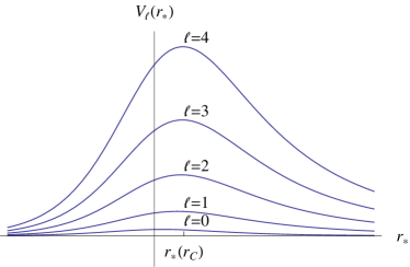
Figure 1: Regge-Wheeler potentials $V_{\ell}(r_{*})$.

One may immediately be concerned that one-dimensional scattering on the real line represents a two-channel problem, while an individual partial wave in three dimensions represents only a single scattering channel. This discrepancy is addressed by imposing appropriate boundary conditions at $r_{*}=\pm\infty$. In the study of black hole thermodynamics, it is instructive to compare results for vacuum states defined through different choices of these boundary conditions; particular cases of interest are the Boulware, Unruh, and Hartle-Hawking vacua. The Boulware vacuum corresponds to a state with no radiation at infinity, but with divergent energy density at $r=2GM$, while the Unruh and Hartle-Hawking vacua avoid this pathology at the expense of introducing radiation at $r=\infty$. The Unruh vacuum corresponds to our expectation for a physical black hole, with an outgoing flux of Hawking radiation at infinity, while the Hartle-Hawking vacuum corresponds to a black hole with outgoing radiation at $r=\infty$ in equilibrium with a corresponding external source of incoming radiation at the same temperature. As a result, we will consider the full one-dimensional scattering problem and later project onto the relevant subspace for a particular problem.

In the standard approach (see for example Refs. Candelas (1980); Candelas and Howard (1984); Anderson (1990); Levi and Ori (2015)), one defines the usual reflection and transmission components of one-dimensional scattering for two channels representing incoming waves from the left and right with the asymptotic behavior

$$\overrightarrow{\phi_{\ell}}(k,r_{*})=\left\{\begin{array}[]{l@{\quad}l}e^{ikr_{*}}+\overrightarrow{A_{\ell}}e^{-ikr_{*}}&r_{*}\to-\infty\cr B_{\ell}e^{ikr_{*}}&r_{*}\to+\infty\end{array}\right.\qquad\hbox{and}\qquad\overleftarrow{\phi_{\ell}}(k,r_{*})=\left\{\begin{array}[]{l@{\quad}l}B_{\ell}e^{-ikr_{*}}&r_{*}\to-\infty\cr e^{-ikr_{*}}+\overleftarrow{A_{\ell}}e^{ikr_{*}}&r_{*}\to+\infty\end{array}\right.\,,$$ (9)

where the transmission coefficient $B_{\ell}$ is the same in both cases. (There has also been more recent work Gray and Visser (2018) applying a formalism based on path-ordered exponentials and transfer matrices.)

For numerical calculations, we will apply methods of analytic scattering theory based on the variable phase approach Calogero (1967); Graham et al. (2002). We will first show how these techniques apply to scattering in the standard basis, and then discuss modifications of this approach that are advantageous for our problem. To begin, we choose an arbitrary “origin” $z_{*,\ell}$. We then define the outgoing wave solution $f_{+,\ell}(k,r_{*})$, which approaches $e^{ikr_{*}}$ as $r_{*}\to+\infty$, and the outgoing wave solution $f_{-,\ell}(k,r_{*})$, which approaches $e^{-ikr_{*}}$ as $r_{*}\to-\infty$. To apply the variable phase method, we parameterize $f_{\pm,\ell}(k,r_{*})=g_{\pm,\ell}(k,r_{*})e^{\pm ikr_{*}}$ and solve for $g_{\pm,\ell}(k,r_{*})$ by integrating Eq. (7) inward from $r_{*}=\pm\infty$, with the boundary condition that $g_{\pm,\ell}(k,r_{*})$ goes to the identity at $r_{*}=\pm\infty$. Since the functions $f_{\pm,\ell}(-k,r_{*})=f_{\pm,\ell}(k,r_{*})^{*}$ also solve the same differential equation, we have a total of four incoming and outgoing wave solutions. To form regular solutions as in Eq. (9), we impose continuity of the wavefunction and first derivative as boundary conditions at $r_{*}=z_{*,\ell}$, together with one additional boundary condition at infinity in each channel: for the regular solution representing scattering of a wave incoming from the left, we require that there be no incident wave from the right, and, similarly, for the regular solution representing scattering of a wave incoming from the right, we require that there be no incident wave from the left.

The equation for $g_{\pm,\ell}(k,r_{*})$ becomes

$$-g_{\pm,\ell}^{\prime\prime}(k,r_{*})-2ikg_{\pm,\ell}(k,r_{*})+v_{\ell}(r_{*})g_{\pm,\ell}(k,r_{*})=0\,,$$ (10)

with boundary conditions at large $|R_{*}|$,

$$g_{+,\ell}(k,R_{*})=\frac{i^{\ell+1}kR_{*}h^{(1)}_{\ell}(kR_{*})}{e^{ikR_{*}}} g_{+,\ell}^{\prime}(k,R_{*})=\frac{i^{\ell+1}k\left((1-ikR_{*}+\ell)h^{(1)}_{\ell}(kR_{*})-kR_{*}h^{(1)}_{\ell+1}(kR_{*})\right)}{e^{ikR_{*}}}$$ (11)

$$g_{-,\ell}(k,-R_{*})=1 g_{-,\ell}^{\prime}(k,-R_{*})=0\,,$$ (12)

where the values for $g_{+,\ell}(k,R_{*})$ represent an improved estimate taking into account the leading behavior of the potential at large $r$, as described in the Appendix. To improve the numerical precision of the calculation, it is also helpful to take advantage of the Wronskian relations between the solutions in each region,

$$g_{\pm,\ell}(k,z_{*,\ell})g_{\pm,\ell}^{\prime}(-k,z_{*,\ell})-g_{\pm,\ell}^{\prime}(k,z_{*,\ell})g_{\pm,\ell}(-k,z_{*,\ell})=2ik\left(g_{\pm,\ell}(k,z_{*,\ell})g_{\pm,\ell}(-k,z_{*,\ell})-1\right)\,,$$ (13)

evaluated at the origin $z_{*,\ell}$.

Using this formalism, we can compute the outgoing wave solutions $f_{\pm,\ell}(k,r_{*})$ and the regular solutions $\overleftarrow{\phi_{\ell}}(k,r_{*})$ and $\overrightarrow{\phi_{\ell}}(k,r_{*})$, along with the $S$-matrix

$$\hat{S}_{\ell}(k)=\begin{pmatrix}B_{\ell}&\overrightarrow{A_{\ell}}\cr\overleftarrow{A_{\ell}}&B_{\ell}\end{pmatrix}\,,$$ (14)

which is unitary for real $k$, and the corresponding eigenphase shifts, which are the eigenvalues of $\frac{1}{2i}\log\hat{S}$. For thermal quantities, the exponential damping due to the Boltzmann factor tends to eliminate subtleties involved with potentially divergent quantities. For example, we can obtain the luminosity of Hawking radiation at infinity as Candelas (1980)

$$L_{\rm tot}=\int_{0}^{\infty}L(k)\,dk=\frac{1}{2\pi}\int_{0}^{\infty}k\sum_{\ell=0}^{\infty}\frac{(2\ell+1)|B_{\ell}(k)|^{2}}{\exp(k/T)-1}dk\,,$$ (15)

where $T=\frac{1}{8\pi GM}$ is the Hawking temperature. As shown in Fig. 2, the variable phase approach yields a calculation that agrees with standard results; roughly, it describes a spectrum that corresponds to the luminosity of Stefan-Boltzmann radiation

$$L_{\rm SB,tot}=\int_{0}^{\infty}L_{\rm SB}(k)\,dk=\int_{0}^{\infty}\frac{27(GM)^{2}k^{3}\,dk}{2\pi(e^{8\pi GMk}-1)}=\frac{9}{40960\pi(GM)^{2}}\,,$$ (16)

at temperature $T$ emitted by a sphere of radius $r=3\sqrt{3}GM$, the geometric-optics limit for the scattering cross section, that is then modified by “gray-body” factors representing the scattering of the outgoing radiation in the Schwarzschild background.

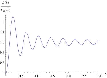
Figure 2: For a massless real scalar field, luminosity of Hawking radiation $L(k)$ at frequency $k$ compared to the luminosity of Stefan-Boltzmann radiation $L_{\rm SB}(k)$ from a blackbody sphere of radius $r=3\sqrt{3}GM$ and temperature $T=\frac{1}{8\pi GM}$. The ratio is plotted as a function of $k$, in units where $2GM=1$.

III Quantum Expectation Values in Curved Spacetime

Renormalized densities can be expressed in terms of sums over the corresponding mode functions. For example, Ref. Candelas (1980) computes the expectation value of $\Phi^{2}$ in the Boulware vacuum as

$$\langle\Phi(r)^{2}\rangle_{B}=\frac{1}{16\pi^{2}r^{2}}\int_{0}^{\infty}\frac{dk}{k}\left[\sum_{\ell=0}^{\infty}(2\ell+1)\left(|\overrightarrow{\phi}_{\ell}(k,r)|^{2}+|\overleftarrow{\phi}_{\ell}(k,r)|^{2}\right)-\frac{4k^{2}r^{2}}{1-\frac{2GM}{r}}\right]-\frac{(GM)^{2}}{48\pi^{2}r^{4}(1-\frac{2GM}{r})}$$ (17)

where the last two terms represent renormalization counterterms, which are found by point-splitting Christensen (1976). The last term is a finite renormalization that arises from the expansion

$$\frac{1}{8\pi^{2}\sigma(\epsilon)}=\frac{1}{4\pi^{2}}\left[\frac{1}{\left(1-\frac{2GM}{r}\right)}\frac{1}{\epsilon^{2}}+\frac{(GM)^{2}}{12r^{4}\left(1-\frac{2GM}{r}\right)}+\frac{(GM)^{3}(4r-7GM)}{240r^{8}\left(1-\frac{2GM}{r}\right)}\epsilon^{2}+{\cal O}(\epsilon^{4})\right]\,,$$ (18)

where $\sigma(\epsilon)$ is the invariant distance squared between the infinitesimally separated points $(t,r,\theta,\varphi)$ and $(t+\epsilon,r,\theta,\varphi)$. The ${\cal O}(\epsilon^{2})$ term in Eq. (18) is not needed for the present calculation, but is included for use below. This expansion is obtained by writing $\sigma(\epsilon)=\frac{1}{2}\sigma_{\mu}(\epsilon)\sigma^{\mu}(\epsilon)$, with Anderson et al. (1995)

$$\sigma^{\mu}(\epsilon)=\delta_{t}^{\mu}\epsilon-\frac{1}{2}\Gamma_{tt}^{\mu}\epsilon^{2}+\frac{1}{6}\Gamma_{tt}^{\rho}\Gamma_{\rho t}^{\mu}\epsilon^{3}-\frac{1}{24}\Gamma_{tt}^{\rho}\left(R^{\mu}_{t\rho t}+\Gamma_{\rho t}^{\lambda}\Gamma_{\lambda t}^{\mu}\right)\epsilon^{4}+\frac{1}{120}\Gamma_{tt}^{r}\left(2\Gamma_{rt}^{\mu}R^{r}_{trt}-\Gamma^{r}_{tt}R^{\mu}_{rtr}+\Gamma^{r}_{tt}\Gamma_{rt}^{t}\Gamma_{rt}^{\mu}\right)\epsilon^{5}+{\cal O}(\epsilon^{6})\,,$$ (19)

where $\Gamma_{\alpha\beta}^{\gamma}$ and $R^{\lambda}_{\alpha\beta\gamma}$ represent the components of the Schwarzschild connection and curvature respectively. The point splitting method then gives the result in Eq. (17) as the limit Candelas (1980)

$$\langle\Phi(r)^{2}\rangle_{B}=\lim_{\epsilon\to 0}\left[\int_{0}^{\infty}\frac{dk}{k}e^{-ik\epsilon}\frac{1}{16\pi^{2}r^{2}}\sum_{\ell=0}^{\infty}(2\ell+1)\left(|\overrightarrow{\phi}_{\ell}(k,r)|^{2}+|\overleftarrow{\phi}_{\ell}(k,r)|^{2}\right)-\frac{1}{8\pi^{2}\sigma(\epsilon)}\right]\,.$$ (20)

As in Ref. Graham et al. (2002), the squared wavefunctions can be re-expressed in terms of the Green’s function at coincident points,

$$|\overrightarrow{\phi}_{\ell}(k,r)|^{2}+|\overleftarrow{\phi}_{\ell}(k,r)|^{2}=2k{\,\rm Im\,}G_{\ell}(r,r,k)\,,$$ (21)

which in turn can be obtained as a product of the regular and outgoing solutions normalized by the Jost function, yielding a form that is amenable to analytic continuation into the upper half-plane.

For numerical calculations of quantities like those in Eq. (17), however, we can anticipate difficulties that arise as a combination of the usual field theory divergences together with the growing strength of the Regge-Wheeler potential for increasing $\ell$. In particular, the sum over partial waves of the Green’s function yields a quadratic divergence in $k$, which then cancels with the first renormalization counterterm. The remaining integral is in principle convergent, but in practice converges only as a result of the cancellation of oscillating contributions in $k$. It is thus not amenable to numerical calculation, but rather can be analyzed in terms of asymptotic limits Candelas (1980) in which one can extract leading analytic behavior.

Motivated by the Born subtraction approach in ordinary quantum field theory Graham et al. (2009), we aim to improve this situation by implementing local subtractions that then allow for a Wick rotation to imaginary wave number; as indicated above, the behavior of the Green’s function in the complex $k$-plane is of interest for its own sake as well. We begin by defining the local spectral density

$$\rho_{\ell}(k,r)=\frac{2k}{i}G_{\ell}(r,r,k)\,,$$ (22)

so that for $k$ real,

$${\,\rm Re\,}\rho_{\ell}(k,r)=|\overrightarrow{\phi}_{\ell}(k,r)|^{2}+|\overleftarrow{\phi}_{\ell}(k,r)|^{2}\,.$$ (23)

While these definitions are written in terms of $r$, in practice we will compute the scattering data in terms of $r_{*}$ and then convert to the corresponding $r$. Using this definition, we rewrite Eq. (17) as

$$\langle\Phi(r)^{2}\rangle_{B} = \frac{1}{16\pi^{2}r^{2}}\int_{0}^{\infty}\frac{dk}{k}\left[\sum_{\ell=0}^{\infty}(2\ell+1){\,\rm Re\,}\rho_{\ell}(k,r)-\frac{4k^{2}r^{2}}{1-\frac{2GM}{r}}\right]-\frac{(GM)^{2}}{48\pi^{2}r^{4}(1-\frac{2GM}{r})}$$ (24)

$$= \frac{1}{32\pi^{2}r^{2}}\int_{-\infty}^{\infty}\frac{dk}{\sqrt{k^{2}}}\left[\sum_{\ell=0}^{\infty}(2\ell+1)\rho_{\ell}(k,r)-\frac{4k^{2}r^{2}}{1-\frac{2GM}{r}}\right]-\frac{(GM)^{2}}{48\pi^{2}r^{4}(1-\frac{2GM}{r})}\,,$$ (25)

where we have used that $\rho_{\ell}(-k,r_{*})=\rho_{\ell}(k,r_{*})^{*}$. However, we must be careful to note a subtlety of this calculation: while the sum over $\ell$ of the real part of $\rho_{\ell}(k,r_{*})$ converges, the sum over the imaginary part does not, even though the contribution from each term cancels between $k$ and $-k$. If we consider the large-$\ell$ limit by setting $k=0$ in Eq. (4), we find Candelas (1980); Candelas and Howard (1984); Anderson (1990); Levi and Ori (2015) that this equation has solutions given by the Legendre functions $P_{\ell}(\xi)$ and $Q_{\ell}(\xi)$, with $\xi=\frac{r}{GM}-1$. Using

$$P_{\ell}(z)Q_{\ell}(z)\approx\frac{1}{\sqrt{z^{2}-1}(2\ell+1)}\hbox{\qquad for $\ell$ large with $z>1$ real,}$$ (26)

and normalizing the solutions using the Wronskian

$$P_{\ell}(z)Q_{\ell}^{\prime}(z)-P_{\ell}^{\prime}(z)Q_{\ell}(z)=\frac{1}{1-z^{2}}\,,$$ (27)

we find that the summand in Eq. (25) approaches the imaginary quantity $\frac{4kr}{i\sqrt{1-\frac{2GM}{r}}}$ for large $\ell$. Thus we can rewrite Eq. (25) as Candelas (1980); Candelas and Howard (1984); Anderson (1990); Levi and Ori (2015)

$$\langle\Phi(r)^{2}\rangle_{B} = \frac{1}{32\pi^{2}r^{2}}\int_{-\infty}^{\infty}\frac{dk}{\sqrt{k^{2}}}\left[\sum_{\ell=0}^{\infty}(2\ell+1)\left(\rho_{\ell}(k,r)-\frac{4kr^{2}}{iGM}P_{\ell}(\xi)Q_{\ell}(\xi)\right)-\frac{4k^{2}r^{2}}{1-\frac{2GM}{r}}\right]-\frac{(GM)^{2}}{48\pi^{2}r^{4}(1-\frac{2GM}{r})}$$ (28)

$$= \frac{1}{32\pi^{2}r^{2}}\int_{-\infty}^{\infty}\frac{dk}{\sqrt{k^{2}}}\left[\sum_{\ell=0}^{\infty}\left((2\ell+1)\rho_{\ell}(k,r)-\frac{4kr}{i\sqrt{1-\frac{2GM}{r}}}\right)-\frac{4k^{2}r^{2}}{1-\frac{2GM}{r}}\right]-\frac{(GM)^{2}}{48\pi^{2}r^{4}(1-\frac{2GM}{r})}\,,$$ (29)

where we have used the identity Candelas and Howard (1984)

$$\sum_{\ell=0}^{\infty}\left[(2\ell+1)P_{\ell}(\xi)Q_{\ell}(\xi)-\frac{1}{\sqrt{\xi^{2}-1}}\right]=0$$ (30)

to equate these two expressions. The subtraction we have introduced in Eq. (29) does not change our original result, since it is purely imaginary and its contribution cancels between $-k$ and $+k$, but the the sums over $\ell$ in Eq. (29) are now convergent.

The subtraction linear in $k$ in Eq. (29) cancels the quadratic divergence in the mode sum. However, this cancellation of large quantities is still ill-behaved numerically; we would strongly prefer to implement this subtraction term by term. We do so by adding and subtracting the leading WKB approximation Candelas and Howard (1984); Maassen van den Brink (2004)

$$\rho_{\ell}^{\rm WKB}(k,r)=\frac{2r^{2}k}{iGM\chi_{\ell}(k,r)}\hbox{\qquad with \qquad}\chi_{\ell}(k,r)=\frac{rk}{iGM}\sqrt{\left(\ell+\frac{1}{2}\right)^{2}\left(1-\frac{2GM}{r}\right)\left(\frac{i}{k}\right)^{2}+r^{2}}$$ (31)

so that Eq. (29) becomes

$$\langle\Phi(r)^{2}\rangle_{B} = \frac{1}{32\pi^{2}r^{2}}\int_{-\infty}^{\infty}\frac{dk}{\sqrt{k^{2}}}\left[\sum_{\ell=0}^{\infty}(2\ell+1)\left(\rho_{\ell}(k,r)-\rho_{\ell}^{\rm WKB}(k,r)\right)\right.$$ (33)

$$\qquad\left.+\sum_{\ell=0}^{\infty}\left((2\ell+1)\rho_{\ell}^{\rm WKB}(k,r)-\frac{4kr}{i\sqrt{1-\frac{2GM}{r}}}\right)-\frac{4k^{2}r^{2}}{1-\frac{2GM}{r}}\right]-\frac{(GM)^{2}}{48\pi^{2}r^{4}(1-\frac{2GM}{r})}\,.$$

As shown in Ref. Candelas and Howard (1984), by turning the sum over $\ell$ into a contour integral, we obtain

$$u(k,r)=\sum_{\ell=0}^{\infty}\left((2\ell+1)\rho^{\rm WKB}_{\ell}(k,r)-\frac{4kr}{i\sqrt{1-\frac{2GM}{r}}}\right)-\frac{4k^{2}r^{2}}{1-\frac{2GM}{r}}=\frac{8kr}{i\sqrt{1-\frac{2GM}{r}}}\int_{0}^{\Lambda(k,r)}\frac{\lambda\,d\lambda}{(e^{2\pi\lambda}+1)\sqrt{\Lambda(k,r)^{2}-\lambda^{2}}}$$ (34)

with

$$\Lambda(k,r)=\frac{k}{i}\frac{r}{\sqrt{1-\frac{2GM}{r}}}\,,$$ (35)

and so we have

$$\langle\Phi(r)^{2}\rangle_{B}=\frac{1}{32\pi^{2}r^{2}}\int_{-\infty}^{\infty}\frac{dk}{\sqrt{k^{2}}}\left[u(k,r)+\sum_{\ell=0}^{\infty}(2\ell+1)\left(\rho_{\ell}(k,r)-\rho_{\ell}^{\rm WKB}(k,r)\right)\right]-\frac{(GM)^{2}}{48\pi^{2}r^{4}(1-\frac{2GM}{r})}\,.$$ (36)

Closing the contour in the upper-half plane, we can then convert this expression into an integral along the branch cut on the imaginary axis $k=i\kappa$,

$$\langle\Phi(r)^{2}\rangle_{B}=\frac{1}{32\pi^{2}r^{2}}\int_{0}^{\infty}\frac{d\kappa}{\kappa}\left[u(i\kappa,r)+\sum_{\ell=0}^{\infty}(2\ell+1)\left(\rho_{\ell}(i\kappa,r)-\rho_{\ell}^{\rm WKB}(i\kappa,r)\right)\right]-\frac{(GM)^{2}}{48\pi^{2}r^{4}(1-\frac{2GM}{r})}\,.$$ (37)

Although this form can in principle be used directly for numerical calculations, an additional subtraction introduced in Ref. Candelas and Howard (1984) significantly improves its convergence. This change consists of subtracting the leading contribution to the second-order WKB approximation along with the first order WKB subtraction, and again adding this contribution back as a contour integral, which can be also expressed in a numerically tractable form. Doing so, we can use the identity Candelas and Howard (1984)

$$\sum_{\ell=0}^{\infty}(2\ell+1)\frac{2r^{2}\kappa}{8GM\chi_{\ell}(i\kappa,r)^{3}}=-\frac{(GM)^{2}}{r^{2}\left(1-\frac{2GM}{r}\right)}{\,\rm Re\,}\int_{0}^{\pi}\frac{\tanh\left[\frac{(e^{i\theta}-1)\pi\kappa r}{\sqrt{1-\frac{2GM}{r}}}\right]\sin\frac{\theta}{2}}{\left(2-e^{i\theta}\right)^{3/2}}\,d\theta$$ (38)

to obtain

$$\langle\Phi(r)^{2}\rangle_{B}=\frac{1}{32\pi^{2}r^{2}}\int_{0}^{\infty}\frac{d\kappa}{\kappa}\left[\tilde{u}(i\kappa,r)+\sum_{\ell=0}^{\infty}(2\ell+1)\left(\rho_{\ell}(i\kappa,r)-\tilde{\rho}_{\ell}^{\rm WKB}(i\kappa,r)\right)\right]-\frac{(GM)^{2}}{48\pi^{2}r^{4}(1-\frac{2GM}{r})}\,,$$ (39)

with

$$\tilde{\rho}_{\ell}^{\rm WKB}(i\kappa,r)=\frac{2r^{2}\kappa}{GM\chi_{\ell}(i\kappa,r)}\left(1+\frac{1}{8\chi_{\ell}(i\kappa,r)^{2}}\right)$$ (40)

and

$$\tilde{u}(i\kappa,r) = \sum_{\ell=0}^{\infty}\left((2\ell+1)\tilde{\rho}^{\rm WKB}_{\ell}(i\kappa,r)-\frac{4\kappa r}{\sqrt{1-\frac{2GM}{r}}}\right)+\frac{4\kappa^{2}r^{2}}{1-\frac{2GM}{r}}$$ (41)

$$= \frac{4r^{2}\kappa^{2}}{1-\frac{2GM}{r}}\int_{0}^{\pi}\frac{\sin\frac{\theta}{2}\,d\theta}{\exp\left(\frac{2\pi\kappa r}{\sqrt{1-\frac{2GM}{r}}}\sin\frac{\theta}{2}\right)+1}-\frac{(GM)^{2}}{r^{2}\left(1-\frac{2GM}{r}\right)}{\,\rm Re\,}\int_{0}^{\pi}\frac{\tanh\left[\frac{(e^{i\theta}-1)\pi\kappa r}{\sqrt{1-\frac{2GM}{r}}}\right]\sin\frac{\theta}{2}}{\left(2-e^{i\theta}\right)^{3/2}}\,d\theta\,,$$ (42)

where we have also substituted $\displaystyle\lambda=\frac{\kappa r}{\sqrt{1-\frac{2GM}{r}}}\sin\frac{\theta}{2}$ in the first term to bring the integrals into a similar form. As described in Ref. Candelas and Howard (1984), these integrals are then straightforward to compute numerically.

IV Computational Scattering Theory Formalism

In the standard scattering basis of Eq. (9), we can write the spectral density in terms of regular and outgoing solutions as

$$\rho_{\ell}(k,r_{*})=f_{+,\ell}(k,r_{*})\overleftarrow{\phi_{\ell}}(k,r_{*})+f_{-,\ell}(-k,r_{*})\overrightarrow{\phi_{\ell}}(k,r_{*})\,.$$ (43)

However, especially for complex $k$, this form can lead to problems in numerical calculation, because it requires integrating one of the outgoing wave solutions through the peak of the Regge-Wheeler potential, which for large $\ell$ becomes strongly repulsive. Although this feature presents a challenge for any numerical computation, the numerical behavior can be improved by switching from a basis consisting of left- and right-moving wavefunctions to a basis of symmetric and antisymmetric wavefunctions. In this approach, the outgoing wave solution and the regular solution are each given by a single $2\times 2$ matrix-valued function that is defined only for $r_{*}\geq z_{*,\ell}$. The four entries of these matrices then represent the symmetric and antisymmetric components of the wavefunctions in the symmetric and antisymmetric scattering channels. The asymmetric potential is then decomposed into a symmetric component, which acts within the symmetric and antisymmetric channels, and an antisymmetric component, which mixes the two channels. Analogously to a spherical problem, where the mixing would be given in terms of Wigner 3-$j$ symbols, this mixing is governed by the overlap integrals of three normalized wavefunctions, which in this case are all equal to zero or $\pm 1$.

The key advantage of this basis is that the variable phase calculation can then be reformulated in terms of a combination of the outgoing wave solution, which is integrated in from infinity, and the regular solution, which is integrated out from the origin Graham et al. (2002); Forrow and Graham (2012); Graham (2014). The resulting improvement in the numerical behavior makes the calculations of the previous section tractable, although in practice it remains helpful to use quadruple precision arithmetic. The detailed algorithm is given in the Appendix. Using this approach, in Fig. 3 we graph

$$\Delta(r) = (2GM)^{2}\left(\langle\Phi(r)^{2}\rangle_{B}+\frac{(GM)^{2}}{48\pi^{2}r^{4}(1-\frac{2GM}{r})}\right)$$ (44)

$$= \frac{(2GM)^{2}}{32\pi^{2}r^{2}}\int_{0}^{\infty}\frac{d\kappa}{\kappa}\left[\tilde{u}(i\kappa,r)+\sum_{\ell=0}^{\infty}(2\ell+1)\left(\rho_{\ell}(i\kappa,r)-\tilde{\rho}_{\ell}^{\rm WKB}(i\kappa,r)\right)\right]\,,$$ (45)

which gives a dimensionless representation of the right-hand side of Eq. (39) without the finite renormalization; this term remains finite at the event horizon $r=2GM$.

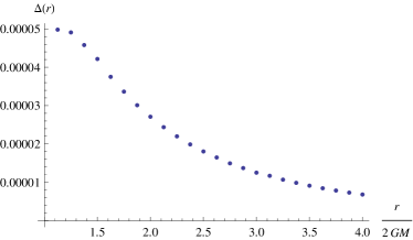
Figure 3: Plot of $\Delta(r)=(2GM)^{2}\left(\langle\Phi(r)^{2}\rangle_{B}+\frac{(GM)^{2}}{48\pi^{2}r^{4}(1-\frac{2GM}{r})}\right)$ as a function of $r$, in units where $2GM=1$.

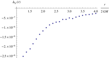
Figure 4: Plot of $\Delta_{k^{2}}(r)=(2GM)^{4}\left(\langle\dot{\Phi}(r)^{2}\rangle_{B}+\frac{(GM)^{3}(4r-7GM)}{480\pi^{2}r^{8}(1-\frac{2GM}{r})}\right)$ as a function of $r$, in units where $2GM=1$.

By applying $-\frac{d^{2}}{d\epsilon^{2}}$ before taking $\epsilon\to 0$ in Eq. (20), we can similarly write the expectation value of $\langle\dot{\Phi}(r)^{2}\rangle_{B}$, where dot denotes the derivative with respect to $t$, as

$$\langle\dot{\Phi}(r)^{2}\rangle_{B}=\frac{1}{16\pi^{2}r^{2}}\int_{0}^{\infty}kdk\left[\sum_{\ell=0}^{\infty}(2\ell+1)\left(|\overrightarrow{\phi}_{\ell}(k,r)|^{2}+|\overleftarrow{\phi}_{\ell}(k,r)|^{2}\right)-\frac{4k^{2}r^{2}}{1-\frac{2GM}{r}}\right]+\frac{(GM)^{3}(4r-7GM)}{480\pi^{2}r^{8}(1-\frac{2GM}{r})}\,,$$ (46)

which we can then calculate via the same approach, yielding

$$\langle\dot{\Phi}(r)^{2}\rangle_{B}=-\frac{1}{32\pi^{2}r^{2}}\int_{0}^{\infty}\kappa d\kappa\left[\tilde{u}(i\kappa,r)+\sum_{\ell=0}^{\infty}(2\ell+1)\left(\rho_{\ell}(i\kappa,r)-\tilde{\rho}_{\ell}^{\rm WKB}(i\kappa,r)\right)\right]+\frac{(GM)^{3}(4r-7GM)}{480\pi^{2}r^{8}(1-\frac{2GM}{r})}\,.$$ (47)

Again in this case it is helpful to define a quantity proportional to the expectation value without the finite renormalization,

$$\Delta_{k^{2}}(r)=(2GM)^{4}\left(\langle\dot{\Phi}(r)^{2}\rangle_{B}-\frac{(GM)^{3}(4r-7GM)}{480\pi^{2}r^{8}(1-\frac{2GM}{r})}\right)\,,$$ (48)

which is shown in Fig. 4. Other contributions to the stress-energy tensor Howard and Candelas (1984) are given by similar calculations, but those cases require additional modifications of the WKB subtraction procedure used above.

V Discussion

We have shown how to use a multichannel variable phase method to compute scattering data for Regge-Wheeler potentials arising from quantum fluctuations in Schwarzschild spacetime. In each channel, this approach uses a basis of symmetric and antisymmetric waves, which are coupled by the asymmetric potential. These techniques are applicable to a broad range of problems involving wave scattering in an asymptotically flat curved spacetime background, including cases where the frequency becomes complex, such as quasi-normal modes or thermal field theory. This approach can also potentially be applied to other geometries that still allow for a partial wave decomposition of the fluctuation spectrum, such as cosmic string spacetimes Allen and Ottewill (1990). Extensions of this calculation to the stress-energy tensor could also offer the opportunity to explore energy condition violation in the Schwarzschild background Visser (1996a, b, c, 1997); pointwise conditions on $\langle T_{\mu\nu}\rangle$ that are strong enough to rule out exotic phenomena such as closed timelike curves, traversable wormholes, and superluminal communication Penrose (1965); Hawking (1965); Tipler (1979); Roman (1986) are typically violated by quantum effects, but motivated by quantum inequalities Ford (1991); Ford and Roman (1995) and information-theoretic arguments, weaker averaged conditions may remain viable in flat Graham and Olum (2005); Fewster et al. (2007); Kelly and Wall (2014); Bousso et al. (2016); Hartman et al. (2017) and curved Graham and Olum (2007); Wall (2010); Kontou and Olum (2013, 2015) spacetime.

Because scattering theory methods are restricted to asymptotically flat spacetimes, they apply to cases in which it is possible to consider global quantities as well. They are given in terms of the global density of states, which in turn is related to the scattering phase shift in each channel. As shown in the Appendix, computing this quantity requires greater care than in standard scattering theory because one cannot easily separate the angular momentum barrier from the potential; as a result, the potential falls off only as the inverse square of distance at large positive $r_{*}$, and the additional phase shift due to the angular momentum barrier, represented by the phase difference of $\ell\pi/2$ between the spherical Hankel function and the ordinary exponential at large distances, shows up as a modification of Levinson’s theorem for the phase shift at $k=0$.

VI Acknowledgments

It is a pleasure to thank E. N. Blose and N. Sadeh for assistance in an earlier stage of this project, and R. L. Jaffe, M. Kardar, and K. Olum for discussions. N. G. was supported in part by the National Science Foundation (NSF) through grants PHY-1520293 and PHY-1820700.

Appendix A Symmetric/Antisymmetric wave basis

In this Appendix we describe the technical details of the scattering calculation using the basis of symmetric and antisymmetric wavefunctions around $z_{*,\ell}$. In this approach, all of the scattering functions become $2\times 2$ matrices, defined only for $r_{*}\geq z_{*,\ell}$, with the actual wavefunction given by one-half the sum of the symmetric and antisymmetric components for $r_{*}>z_{*,\ell}$ and one-half the difference for $r_{*}<z_{*,\ell}$. In this basis, the asymmetric Regge-Wheeler potential contains off-diagonal terms mixing these two channels, analogously to the case of asymmetric objects in a spherical basis Forrow and Graham (2012) (the analogs of the 3-$j$ symbols are zero or $\pm 1$). Again using the variable phase method, we now obtain a single matrix-valued outgoing wave solution and, by applying boundary conditions at $z_{*,\ell}$, the corresponding matrix-valued regular solution. A key advantage of this approach is that we can take advantage of the inward/outward parameterization developed in Ref. Graham et al. (2002).

We take as the arbitrary “origin” the value of $r_{*}$ corresponding to the leading estimate for the maximum of the Regge-Wheeler potential, $z_{*,\ell}=r_{*}(r_{\ell}^{\rm peak})$, where Boonserm and Visser (2008)

$$r_{\ell}^{\rm peak}=3GM\left(1-\frac{1}{9\ell(\ell+1)}\right)\hbox{\quad for $\ell\neq 0$, and \quad}r_{0}^{\rm peak}=\frac{8GM}{3}\hbox{\quad for $\ell=0$.}$$ (49)

We work with matrix wavefunctions $\hat{\psi}_{\ell}(k,r_{*})$ that are defined only for $r_{*}\geq z_{*,\ell}$; to obtain the actual scalar wavefunction, we project out the value on the left or right of the “origin” by

$$\psi_{\ell}(k,r_{*})=\left\{\begin{array}[]{ll}{\,\rm tr\,}\left[\hat{P}_{-}\hat{\psi}_{\ell}(k,2z_{*,\ell}-r_{*})\right]&r_{*}<z_{*,\ell}\\ {\,\rm tr\,}\left[\hat{P}_{+}\hat{\psi}_{\ell}(k,r_{*})\right]&r_{*}\geq z_{*,\ell}\\ \end{array}\right.\,,$$ (50)

with $\hat{P}_{\pm}=\frac{1}{2}\begin{pmatrix}1&\pm 1\cr\pm 1&1\end{pmatrix}$.

Following Graham et al. (2002); Forrow and Graham (2012); Graham (2014), we parameterize the matrix outgoing wave solution to Eq. (7) as

$$\hat{\psi}_{\ell}^{\rm out}(k,r_{*})=e^{ikr_{*}}\hat{g}_{\ell}(k,r_{*})\,,$$ (51)

where we have factored out the free wavefunction $e^{ikr_{*}}$. Then $\hat{g}_{\ell}(k,r_{*})$ obeys the differential equation

$$-\hat{g}_{\ell}^{\prime\prime}(k,r_{*})-2ik\hat{g}_{\ell}^{\prime}(k,r_{*})+\hat{v}_{\ell}(r_{*})\hat{g}_{\ell}(k,r_{*})=0\,,$$ (52)

where prime denotes derivative with respect to $r_{*}$ and the elements of the potential matrix are given by

$$\hat{v}_{\ell}(r_{*})_{bc}=\sum_{a=1}^{2}\left(\frac{V_{\ell}(r_{*})+(-1)^{a}V_{\ell}(2z_{*,\ell}-r_{*})}{2}\right)\left(\frac{(-1)^{a+b+c}+1}{2}\right)\,.$$ (53)

Here $a=1$ is the antisymmetric channel and $a=2$ is the symmetric channel. Imposing outgoing wave boundary conditions for $r_{*}\to\infty$, we formally would have $\hat{g}_{\ell}(k,r_{*}\to\infty)=\hat{1}$ and $\hat{g}_{\ell}^{\prime}(k,r_{*}\to\infty)=\hat{0}$. However, because of the slow falloff of the potential, for the large but finite $r_{*}$ that arise in numerical calculations, it is advantageous to use a better estimate of the outgoing wavefunctions for large $r_{*}$. On the right the wavefunction approaches the spherical Hankel function solution $i^{\ell+1}kr_{*}h^{(1)}_{\ell}(kr_{*})$, while on the left the wavefunction approaches the exponential solution used above. As a result, in the matrix formalism a better estimate at $r_{*}=R_{*}$ for large positive $R_{*}$ is given by

$$\hat{g}_{\ell}(k,R_{*})=\frac{1}{2}\left[\frac{i^{\ell+1}kR_{*}h^{(1)}_{\ell}(kR_{*})}{e^{ikR_{*}}}\begin{pmatrix}1&1\cr 1&1\end{pmatrix}+\begin{pmatrix}1&-1\cr-1&1\end{pmatrix}\right]\,,$$ (54)

and correspondingly, after some simplification,

$$\hat{g}_{\ell}^{\prime}(k,R_{*})=\frac{i^{\ell+1}k\left((1-ikR_{*}+\ell)h^{(1)}_{\ell}(kR_{*})-kR_{*}h^{(1)}_{\ell+1}(kR_{*})\right)}{2e^{ikR_{*}}}\begin{pmatrix}1&1\cr 1&1\end{pmatrix}\,.$$ (55)

Again following Refs. Graham et al. (2002); Forrow and Graham (2012); Graham (2014), we can parameterize the regular solution as

$$\hat{\psi}_{\ell}^{\rm reg}(k,r_{*})=e^{-ik(r_{*}-z_{*,\ell})}\hat{h}_{\ell}(k,r_{*})\,,$$ (56)

where $\hat{h}_{\ell}(k,r_{*})$ obeys the differential equation (note the reversed order of the matrix multiplication in the potential term)

$$-\hat{h}_{\ell}^{\prime\prime}(k,r_{*})+2ik\hat{h}_{\ell}^{\prime}(k,r_{*})+\hat{h}_{\ell}(k,r_{*})\hat{v}_{\ell}(r_{*})=0\,.$$ (57)

The regular solution obeys boundary conditions at the “origin” $z_{*,\ell}$ such that the function and first derivative match the solution in the absence of the potential,

$$\hat{h}_{\ell}^{\rm free}(k,r_{*})=\frac{e^{ik(r_{*}-z_{*,\ell})}}{k}\begin{pmatrix}\sin k(r_{*}-z_{*,\ell})&0\cr 0&\frac{1}{i}\cos k(r_{*}-z_{*,\ell})\end{pmatrix}\,.$$ (58)

In terms of these functions, the matrix-valued local spectral density in the symmetric/antisymmetric matrix basis is given by

$$\hat{\rho}_{\ell}(k,r_{*})=4ik\hat{F}_{\ell}(k)^{-1}\hat{h}_{\ell}(k,r_{*})\hat{g}_{\ell}(k,r_{*})\,,$$ (59)

where the matrix-valued Jost function $\hat{F}_{\ell}(k)$ is given in terms of the Wronskian of the regular and outgoing solutions as

$$\hat{F}_{\ell}(k)=2ik\hat{h}_{\ell}(k,x_{*})\hat{g}_{\ell}(k,x_{*})+\hat{h}_{\ell}(k,x_{*})\hat{g}_{\ell}^{\prime}(k,x_{*})-\hat{h}^{\prime}(k,x_{*})\hat{g}_{\ell}(k,x_{*})\,,$$ (60)

which can be evaluated at any fitting point $x_{*}$; we choose $x_{*}=r_{*}$ so that no new calculation is necessary. The scalar spectral density of Eq. (22) is then obtained using the same projection procedure as that described in Eq. (50) above for the scattering wavefunctions. We note that on the imaginary $k$-axis, the Jost function matrix can become ill-conditioned for large $\ell$, so we compute the matrix inverse using a singular value decomposition.

Although it is not needed in the calculation of local densities, we can also use the Jost function to obtain the $S$-matrix as

$$\hat{S}_{\ell}(k)=\hat{F}_{\ell}(k)^{-1}\hat{M}\hat{F}_{\ell}(-k)\hat{M}$$ (61)

where $\hat{M}$ is the constant matrix $\hat{M}=\begin{pmatrix}-1&0\\ 0&1\end{pmatrix}$. We can then obtain the total phase shift as

$$\delta_{\ell}(k)=\frac{1}{2i}\log\det\hat{S}_{\ell}(k)$$ (62)

which is in turn related to the global density of states by

$$\rho_{\ell}(k)=\frac{1}{\pi}\frac{d\delta_{\ell}}{dk}\,.$$ (63)

In order to resolve ambiguities in the branch cut of the logarithm, we define $\beta_{\ell}(k,r_{*})=\log\det\hat{g}_{\ell}(k,r_{*})$, which we can calculate by solving

$$\beta_{\ell}^{\prime}(k,r_{*})=\frac{1}{2i}{\,\rm tr\,}\hat{g}_{\ell}^{\prime}(k,r_{*})\hat{g}_{\ell}(k,r_{*})^{-1}$$ (64)

subject to the boundary condition $\beta_{\ell}(k,R_{*})=0$. Then by choosing the branch of the logarithm such that $|\delta_{\ell}(k)-\beta_{\ell}(k,z_{*,\ell})|<\pi$, we obtain a continuous phase shift that goes to zero for $k\to\infty$. We note that at $k=0$, the phase shift goes to $-\pi(\ell+1)/2$. This result differs from the behavior of a standard potential in one dimension, which would approach $-\pi/2$ for a repulsive potential, because of the leading $\ell(\ell+1)/r_{*}^{2}$ behavior of the potential at large positive $r_{*}$; the difference of $\ell\pi/2$ corresponds to the phase shift of the spherical Hankel function compared to the ordinary exponential.

References

- Regge and Wheeler (1957) T. Regge and J. A. Wheeler, Phys. Rev. 108, 1063 (1957).
- Sanchez (1976) N. G. Sanchez, J. Math. Phys. 17, 688 (1976).
- Sanchez (1977) N. G. Sanchez, Phys. Rev. D 16, 937 (1977).
- Sanchez (1978) N. G. Sanchez, Phys. Rev. D 18, 1030 (1978).
- Ferrari and Mashhoon (1984) V. Ferrari and B. Mashhoon, Phys. Rev. Lett. 52, 1361 (1984).
- Matzner et al. (1985) R. A. Matzner, C. DeWitte-Morette, B. Nelson, and T.-R. Zhang, Phys. Rev. D 31, 1869 (1985).
- Anninos et al. (1992) P. Anninos, C. DeWitt-Morette, R. A. Matzner, P. Yioutas, and T. R. Zhang, Phys. Rev. D 46, 4477 (1992).
- Andersson (1995) N. Andersson, Phys. Rev. D 52, 1808 (1995).
- Kokkotas and Schmidt (1999) K. D. Kokkotas and B. Schmidt, Living Reviews in Relativity 2 (1999).
- Motl and Neitzke (2003) L. Motl and A. Neitzke, Adv. Theor. Math. Phys. 7, 307 (2003).
- van den Brink (2004) A. M. van den Brink, Journal of Mathematical Physics 45, 327 (2004).
- Dolan et al. (2006) S. Dolan, C. Doran, and A. Lasenby, Phys. Rev. D 74, 064005 (2006).
- Dolan and Ottewill (2011) S. R. Dolan and A. C. Ottewill, Phys. Rev. D 84, 104002 (2011).
- Konoplya and Zhidenko (2011) R. A. Konoplya and A. Zhidenko, Rev. Mod. Phys. 83, 793 (2011).
- Batic et al. (2012) D. Batic, N. G. Kelkar, and M. Nowakowski, Phys. Rev. D 86, 104060 (2012).
- Raffaelli (2013) B. Raffaelli, Journal of High Energy Physics 2013, 188 (2013).
- Candelas (1980) P. Candelas, Phys. Rev. D 21, 2185 (1980).
- Giddings (2016) S. B. Giddings, Phys. Lett. B 754, 39 (2016).
- Page (1982) D. N. Page, Phys. Rev. D 25, 1499 (1982).
- Candelas and Howard (1984) P. Candelas and K. W. Howard, Phys. Rev. D 29, 1618 (1984).
- Howard and Candelas (1984) K. W. Howard and P. Candelas, Phys. Rev. Lett. 53, 403 (1984).
- Jensen and Ottewill (1989) B. P. Jensen and A. Ottewill, Phys. Rev. D 39, 1130 (1989).
- Anderson (1990) P. R. Anderson, Phys. Rev. D 41, 1152 (1990).
- Anderson et al. (1993) P. R. Anderson, W. A. Hiscock, and D. A. Samuel, Phys. Rev. Lett. 70, 1739 (1993).
- Anderson et al. (1995) P. R. Anderson, W. A. Hiscock, and D. A. Samuel, Phys. Rev. D 51, 4337 (1995).
- Sushkov (2000) S. V. Sushkov, Phys. Rev. D 62, 064007 (2000).
- Popov (2003) A. A. Popov, Phys. Rev. D 67, 044021 (2003).
- Levi and Ori (2015) A. Levi and A. Ori, Phys. Rev. D 91, 104028 (2015).
- Lambert (1758) J. H. Lambert, Acta Helvetica 3, 128 (1758).
- Euler (1783) L. Euler, Acta Academiae Scientiarum Imperialis Petropolitanae 2, 29 (1783).
- Corless et al. (1996) R. M. Corless, G. H. Gonnet, D. E. Hare, D. J. Jeffrey, and D. E. Knuth, Advances in Computational Mathematics 5, 329 (1996).
- Gray and Visser (2018) F. Gray and M. Visser, Universe 4, 93 (2018).
- Calogero (1967) F. Calogero, Variable Phase Approach to Potential Scattering (Academic Press, New York, 1967).
- Graham et al. (2002) N. Graham, R. L. Jaffe, V. Khemani, M. Quandt, M. Scandurra, and H.Weigel, Nucl. Phys. B645, 49 (2002).
- Christensen (1976) S. M. Christensen, Phys. Rev. D 14, 2490 (1976).
- Graham et al. (2009) N. Graham, M. Quandt, and H. Weigel, Spectral Methods in Quantum Field Theory (Springer-Verlag, Berlin, 2009).
- Maassen van den Brink (2004) A. Maassen van den Brink, J. Math. Phys. 45, 327 (2004).
- Forrow and Graham (2012) A. Forrow and N. Graham, Phys. Rev. A 86, 062715 (2012).
- Graham (2014) N. Graham, Phys. Rev. A 90, 032507 (2014).
- Allen and Ottewill (1990) B. Allen and A. C. Ottewill, Phys. Rev. D 42, 2669 (1990).
- Visser (1996a) M. Visser, Phys. Rev. D 54, 5103 (1996a).
- Visser (1996b) M. Visser, Phys. Rev. D 54, 5116 (1996b).
- Visser (1996c) M. Visser, Phys. Rev. D 54, 5123 (1996c).
- Visser (1997) M. Visser, Phys. Rev. D 56, 936 (1997).
- Penrose (1965) R. Penrose, Phys. Rev. Lett. 14, 57 (1965).
- Hawking (1965) S. W. Hawking, Phys. Rev. Lett. 15, 689 (1965).
- Tipler (1979) F. J. Tipler, General Relativity and Gravitation 10, 985 (1979).
- Roman (1986) T. A. Roman, Phys. Rev. D 33, 3526 (1986).
- Ford (1991) L. H. Ford, Phys. Rev. D 43, 3972 (1991).
- Ford and Roman (1995) L. H. Ford and T. A. Roman, Phys. Rev. D 51, 4277 (1995).
- Graham and Olum (2005) N. Graham and K. D. Olum, Phys. Rev. D 72, 025013 (2005).
- Fewster et al. (2007) C. J. Fewster, K. D. Olum, and M. J. Pfenning, Phys. Rev. D 75, 025007 (2007).
- Kelly and Wall (2014) W. R. Kelly and A. C. Wall, Phys. Rev. D 90, 106003 (2014).
- Bousso et al. (2016) R. Bousso, Z. Fisher, J. Koeller, S. Leichenauer, and A. C. Wall, Phys. Rev. D 93, 024017 (2016).
- Hartman et al. (2017) T. Hartman, S. Kundu, and A. Tajdini, JHEP 07, 066 (2017).
- Graham and Olum (2007) N. Graham and K. D. Olum, Phys. Rev. D 76, 064001 (2007).
- Wall (2010) A. C. Wall, Phys. Rev. D 81, 024038 (2010).
- Kontou and Olum (2013) E.-A. Kontou and K. D. Olum, Phys. Rev. D 87, 064009 (2013).
- Kontou and Olum (2015) E.-A. Kontou and K. D. Olum, Phys. Rev. D 92, 124009 (2015).
- Boonserm and Visser (2008) P. Boonserm and M. Visser, Phys. Rev. D 78, 101502 (2008).