Measures of path-based nonlinear expansion rates and Lagrangian uncertainty in stochastic flows

Abstract.

We develop a probabilistic characterisation of trajectorial expansion rates in non-autonomous stochastic dynamical systems that can be defined over a finite time interval and used for the subsequent uncertainty quantification in Lagrangian (trajectory-based) predictions. These expansion rates are quantified via certain divergences (pre-metrics) between probability measures induced by the laws of the stochastic flow associated with the underlying dynamics. We construct scalar fields of finite-time divergence/expansion rates, show their existence and space-time continuity for general stochastic flows. Combining these divergence rate fields with information inequalities derived in [17] allows for quantification and mitigation of the uncertainty in path-based observables estimated from simplified models in a way that is amenable to algorithmic implementations, and it can be utilised in information-geometric analysis of statistical estimation and inference, as well as in a data-driven machine/deep learning of coarse-grained models. We also derive a link between the divergence rates and finite-time Lyapunov exponents for probability measures and for path-based observables.

Keywords: Lagrangian uncertainty, stochastic flows, dynamical systems, information inequalities, expansion rates, $\varphi$-divergence rates, Lyapunov exponents.

1. Introduction

Consider a dynamical system on a smooth finite-dimensional manifold $\mathcal{M}$ generated by the map, $\phi_{t_{0},t}\,{:}\;\mathcal{M}\,{\times}\,\Omega\rightarrow\mathcal{M}$, $t\in\mathcal{I}:=[t_{0},\,T\hskip 0.56917pt)$, such that

$$\phi_{t_{0},t_{0}}(\,\cdot\,,\omega)=\textrm{id}_{\mathcal{M}},\quad\phi_{t_{0},t}(\,\cdot\,,\omega)=\phi_{u,t}(\phi_{t_{0},u}(\,\cdot\,,\omega),\omega)\quad\textrm{a.a.}\;\,\omega\in\Omega\quad\forall\,t,u\in\mathcal{I},$$ (1.1)

where $(\Omega,\mathcal{F},\mathbb{P})$ is a complete probability space. It is a basic fact that for any fixed $y$, $x+y\in\mathcal{M}$, and the paths $t\mapsto\phi_{t_{0},t}(x,\omega)$, $t\mapsto\phi_{t_{0},t}(x+y,\omega)$ the distance $\|\phi_{t_{0},t}(x,\omega)-\phi_{t_{0},t}(x+y,\omega)\|$ can be large (on the scale of $\mathcal{M}$) after some finite time even if $|y|\ll 1$. More importantly, it is also well known that for two distinct measurable families of maps $\{\phi_{t_{0},t}^{\mu}\}_{t\in\mathcal{I}}$, $\{\phi^{\nu}_{t_{0},t}\}_{t\in\mathcal{I}}$ generated by difference or differential equations the paths $t\mapsto\phi^{\mu}_{t_{0},t}(x,\omega)$, $t\mapsto\phi^{\nu}_{t_{0},t}(x,\omega)$ can be very different so that $\|\phi_{t_{0},t}^{\mu}(x,\omega)-\phi_{t_{0},t}^{\nu}(x,\omega)\|\gg 1$ $\mathbb{P}$ - a.s. for a non-negligible set of initial conditions $x\in\mathcal{M}$ even if the vector fields generating these maps are arbitrarily $L^{p}$-close (but not identical); see, e.g., [50, 8, 57, 70, 49, 61, 15]) amongst a vast literature concerned with dynamical systems theory. In other words, for a generic dynamical system even small uncertainties in the initial condition or in the underlying dynamics are likely to result in a drastically different fate of the corresponding trajectories/paths and thus lead to significant errors in predictions based on the trajectories of the underlying dynamical system.

Given the paths, $t\mapsto\phi_{t_{0},t}(x,\omega)$, $\omega\in\Omega$, labelled by the (potentially uncertain) initial conditions $x\in\mathcal{M}$, and a measurable functional $f$ on these paths, we refer to the estimation of observables $x\mapsto\mathbb{E}\big{[}f\big{(}\phi_{t_{0},\scaleobj{1.25}{\,\cdot\,}}(x)\big{)}\big{]}$ as a Lagrangian prediction. In contrast, estimation of vector fields generating the family of maps $(\phi_{t_{0},t})_{t\in\mathcal{I}}$ is referred to as an Eulerian prediction; see [17]. This work is motivated by the desire to devise a systematic approach to improving path-based/Lagrangian predictions in complex dynamical systems based on simplified, data-driven models. Thus, our main objective, following on from [17], is to develop a general framework for quantification and mitigation of error in Lagrangian predictions which are obtained from (Eulerian) vector fields generating the underlying dynamical system in a way which naturally applies to both the deterministic and stochastic settings. Importantly, as highlighted above, the effects of uncertainties on the skill of Lagrangian predictions are distinctly different from uncertainties affecting approximations of the Eulerian fields (generating the maps $\{\phi^{\nu}_{t_{0},t}\}_{t\in\mathcal{I}}$) and different ‘metrics’ have to be developed for estimating and mitigating the error in path-based observables. These issues are naturally addressed in the probabilistic setting, where information-theoretic/geometric tools can be used to bound and minimise the lack of information in Lagrangian estimates obtained from uncertain Eulerian fields. The following major steps are needed to achieve this objective:

• Determination of an appropriate measure of discrepancy between two Lagrangian predictions which is analytically and computationally tractable, and such that it can be utilised in information-geometric analysis of statistical estimation and inference on families of models.

• Derivation of bounds on the error in Lagrangian observables estimated from approximate models of the original dynamics, and bounding errors in the underlying probability measures.

• Identification of the most important Lagrangian structures, i.e., subsets of true and approximate trajectories which need to be systematically ‘tuned’ in order to minimise the loss of information in Lagrangian predictions based on approximate Eulerian fields.

A framework addressing (i)-(ii) was developed in [17]. Here, we address step (iii) above and consider fields of trajectorial expansion/divergence rates (around every $x\in\mathcal{M}$) which utilise the evolution of time-marginal probability associated with the (path space) law of the stochastic flow. It turns out minimising the discrepancy between such fields generated by the true dynamics and its approximations can be used to systematically bound the uncertainty the Lagrangian predictions and minimise the error in path space observables. Importantly, this procedure can be carried out within the statistical estimation/inference framework or within a purely data-driven setting. As illustrated later on, the features which models have to reproduce for best Lagrangian prediction skill are generally very different from the Eulerian features one would optimise for when predicting, say, the evolution of velocity fields in atmosphere-ocean science applications. Apart from purely theoretical aspects relevant for finite-dimensional dynamical systems (e.g., [57, 70, 49, 61, 15, 7, 11, 12, 22, 29]), Hamiltonian PDEs, or some parabolic PDEs (e.g., [27, 28]), a major motivation for these efforts arose from the desire to provide Lagrangian/path-based predictions in geophysical flows or in molecular dynamics.

In what follows, we first construct scalar fields of finite-time expansion/divergence rates based on the evolution of time-marginal probability measures associated with projections of path space measures induced by the underlying dynamics. We then focus on the analytical issues related to the existence and properties of such fields. At this stage we do not consider the Lagrangian ‘tuning’ of the divergence rate fields, nor do we focus on approaches to estimating the fields generated by the true dynamics which is, in applications, likely to be only sampled through partial and noisy observations. These practically important but also numerically involved issues are postponed to a subsequent publication devoted to applications. The use of the bound on the discrepancy between the divergence rate fields as a loss function in machine/deep learning of coarse-grained models is of special interest and is a subject on an ongoing work.

The contents of this article are as follows. Section 2 outlines the general setup, the hierarchy of main results and notation. In section 3 we introduce the main tools and background results which are needed for the subsequent derivations. Section 4 is devoted to the main results. The finite-time divergence rates ($\varphi$-DR) are defined in §4.1 and their general properties are outlined in §4.2. Fields of finite-time divergence rates ($\varphi$-DRF) are discussed in §4.3. A tangential but interesting issue concerned with the links between $\varphi$-DRF and the fields of finite-time Lyapunov exponents is discussed in §5. Section 6 is devoted to numerical examples illustrating the finite-time divergence rate fields for several dynamical systems. We close with some remarks on future work in section 7. Several technical proofs are delegated to the Appendix to improve the read.

2. Main results

The setup and the main results of this work are outlined below. Frequently used notation is summarised in the Glossary at the end of the paper.

2.1. Basic setup and notation

For the most part, either for convenience or by necessity, we will assume that the dynamics is generated by the Stratonovich stochastic differential equation (SDE) on $\mathcal{M}$, that is

$$dX_{t}^{t_{0},x}=\mathring{b}\big{(}t,X_{t}^{t_{0},x}\big{)}dt+\sigma\big{(}t,X_{t}^{t_{0},x}\big{)}\circ dW_{t-t_{0}},\qquad X_{t_{0}}^{t_{0},x}\sim\mu_{t_{0}}\in\mathord{\raisebox{-0.95001pt}{\scaleobj{.86}{\includegraphics[width=10.00002pt]{PP.pdf}}}}\hskip 0.56917pt(\mathcal{M}),\quad t\in\mathcal{I}:=[t_{0},\,T\hskip 0.56917pt),$$ (2.1)

where $W_{t}$ is an m-dimensional Wiener process and the uncertainty in the initial conditions, or a distribution of initial conditions of interest, is prescribed by $\mu_{t_{0}}\in\mathord{\raisebox{-0.95001pt}{\scaleobj{.86}{\includegraphics[width=10.00002pt]{PP.pdf}}}}\hskip 0.56917pt(\mathcal{M})$, where $\mathord{\raisebox{-0.95001pt}{\scaleobj{.86}{\includegraphics[width=10.00002pt]{PP.pdf}}}}\hskip 0.56917pt(\mathcal{M})$ is the space of Borel probability measures on $\mathcal{M}$. Throughout, $\mathcal{M}=\mathbb{R}^{d}$ or a flat torus $\mathcal{M}\,{=}\,\bar{\mathbb{T}}^{d}$ and all probability measures defined on the appropriate Borel $\mathfrak{S}$-algebra. In this case $(\Omega,\mathcal{F},\mathbb{P})$ associated with (1.1) is the Wiener probability space and the law of $X_{t}^{t_{0},x}$ is given by ${\mathfrak{P}\hskip 0.28436pt}_{t_{0}}\simeq\mu_{t_{0}}\otimes\mathbb{P}$. Furthermore, $\Omega\simeq\mathcal{C}_{0}(\mathbb{R};\mathbb{R}^{m})$ is identified with a subspace of continuous functions $\mathcal{C}(\mathbb{R};\mathbb{R}^{m})$ which vanish at zero (e.g., [6]), and $\mathbb{P}$ is the Wiener measure on $\mathcal{F}$, where $\mathcal{F}$ is the Borel $\mathfrak{S}$-algebra on $\Omega$ generated by the Wiener process. In what follows, we will consider $(\mathring{b},\sigma)$ such that (2.1) has unique global solutions which can be represented by stochastic flows (§3); namely

$$X^{t_{0},x}_{t}(\omega)=\phi_{t_{0},t}(x,\omega)\quad\mathbb{P}\,\textrm{-\,a.s.}\quad t\in\mathcal{I},\;x\in\mathcal{M}.$$

Under some weak assumptions specified in §3 the family of maps $\big{\{}\phi_{t_{0},t}(\,\cdot\,,\,\cdot\,)\big{\}}_{t\in\mathcal{I}}$ represents a stochastic flow of homeomorphisms on $\mathcal{M}$; we will exploit this fact extensively. Many results derived in the sequel apply to a broader class of flows than those induced by solutions of SDEs in the Markovian setting but the outlined case serves as a useful reference setup.

Given the family of time-marginal probability measures $(\mu_{t})_{t\in\mathcal{I}}$, $\mu_{t}\in\mathord{\raisebox{-0.95001pt}{\scaleobj{.86}{\includegraphics[width=10.00002pt]{PP.pdf}}}}\hskip 0.56917pt(\mathcal{M})$ generated, for example, by the law of $\phi_{t_{0},\scaleobj{1.25}{\,\cdot\,}}$ on $\mathcal{M}$, a unified probabilistic approach to studying trajectorial expansion rates and uncertainty associated with the paths $x\mapsto\phi_{t_{0},t}(x,\omega)$ is based on utilising the so-called $\varphi$-divergencies $D_{\varphi}(\mu_{t}\|\mu_{t_{0}})$ which are defined as

$$\mathcal{D}_{\varphi}(\mu_{t}\|\mu_{t_{0}})=\scaleobj{.9}{\int_{\mathcal{M}}}\,\varphi\big{(}d\mu_{t}/d\mu_{t_{0}}\big{)}d\mu_{t_{0}},$$ (2.2)

where $d\mu_{t}/d\mu_{t_{0}}$ is the Radon-Nikodym derivative, and $\varphi\in\mathcal{C}^{2}(\mathbb{R}^{+})$ is a strictly convex scalar function (see §4). This probabilistic notion of trajectorial expansion rates has an information-theoretic interpretation as the loss of information in the measure $\mu_{t_{0}}$ on the initial conditions for approximating $\mu_{t}$ and it is used in [17] for Lagrangian uncertainty quantification in path-based predictions. Here, we further develop the link between Lagrangian uncertainty and certain fields of $\varphi$-divergences which can be utilised in data-driven model learning and optimization.

2.2. Outline of main results

Our results can be summarised as follows:

• We define and study nonlinear expansion rates, termed the $\varphi$-divergence rates ($\varphi$-DR), which are based on the evolution of time-marginal probability measures $(\mu_{t})_{t\in\mathcal{I}}$, ${\mu_{t}\in\mathord{\raisebox{-0.95001pt}{\scaleobj{.86}{\includegraphics[width=10.00002pt]{PP.pdf}}}}\hskip 0.56917pt(\mathcal{M})}$ in terms of $\mathcal{D}_{\varphi}(\mu_{t}\|\mu_{t_{0}})$. Then, we construct scalar $\varphi$-DR fields, $x\mapsto\mathcal{D}_{\varphi}^{t_{0},t}(\mu^{x}_{t}\|\mu^{x}_{t_{0}})$, where $\mu^{x}_{t_{0}}$ is a probability measure localised around $x\in\mathcal{M}$, and $\mathcal{D}^{t_{0},t}_{\varphi}:=|t-t_{0}|^{-1}\mathcal{D}_{\varphi}$. These fields are defined for any family $(\mu_{t})_{t\in\mathcal{I}}$ such that $\mu_{t}\ll\mu_{t_{0}}$ but we focus on time-marginal measures of the (path space) law ${\mathfrak{P}\hskip 0.28436pt}_{t_{0}}$ of the stochastic flow $\big{\{}\phi_{t_{0},t}\big{\}}_{t\in\mathcal{I}}$ in which case ${\mathfrak{P}\hskip 0.28436pt}_{t_{0}}\circ\phi^{-1}_{t_{0},t}=\mu_{t}$, thus providing a trajectorial interpretation. In section 4 (Theorem 4.12) we show that the $\varphi$-DR fields exist and are space-time continuous under fairly general conditions, and that they provide a computable diagnostic of nonlinear expansion induced by the stochastic flow.

  Importantly, $\varphi$-DR fields can be viewed as a general measure-based diagnostic of the growth of uncertainty in stochastic flows that operates in both the deterministic and the stochastic settings. The information-theoretic loss of information in $\mu^{x}_{t}\in\mathord{\raisebox{-0.95001pt}{\scaleobj{.86}{\includegraphics[width=10.00002pt]{PP.pdf}}}}\hskip 0.56917pt(\mathcal{M})$ for describing the initial probability measure $\mu^{x}_{t_{0}}$ is used in [17] for uncertainty quantification in path-based predictions of statistical observables. These results rely on the hierarchy of bounds on statistical observables based on two different flows, $\{\phi_{t_{0},t}^{\mu}\}_{t\in\mathcal{I}}$ and $\{\phi_{t_{0},t}^{\nu}\}_{t\in\mathcal{I}}$, which employ general information bounds/inequalities in the form

  $$\hat{\mathcal{K}}_{\varphi,f}^{\nu}\big{(}-\mathcal{D}_{\varphi}(\mu_{t}\|\nu_{t})\big{)}\leqslant\mathbb{E}^{\mu_{t}}[f]-\mathbb{E}^{\nu_{t}}[f]\leqslant\mathcal{K}_{\varphi,f}^{\nu}\big{(}\mathcal{D}_{\varphi}(\mu_{t}\|\nu_{t})\big{)},\quad t\in\mathcal{I},$$ (2.3)

  where $\mathbb{E}^{\mu_{t}}[f]=\mathbb{E}^{\mu_{t_{0}}\otimes\mathbb{P}}\big{[}f\big{(}\phi_{t_{0},t}^{\mu}\big{)}\big{]}$, $\mathbb{E}^{\nu_{t}}[f]=\mathbb{E}^{\mu_{t_{0}}\otimes\mathbb{P}}\big{[}f\big{(}\phi_{t_{0},t}^{\nu}\big{)}\big{]}$ (see (3.17)), $\mu_{t},\nu_{t}\in\mathord{\raisebox{-0.95001pt}{\scaleobj{.86}{\includegraphics[width=10.00002pt]{PP.pdf}}}}\hskip 0.56917pt(\mathcal{M})$, and $\mathcal{K}_{\varphi,f}^{\nu}$, $\hat{\mathcal{K}}_{\varphi,f}^{\nu}$ are bounded and such that $\mathcal{K}_{\varphi,f}^{\nu}(u)\rightarrow 0$, $\hat{\mathcal{K}}_{\varphi,f}^{\nu}(-u)\rightarrow 0$ as $u\,{\downarrow}\,0$. In particular, setting $f=\textrm{Id}_{\mathscr{A}}$ corresponds to estimating the fate of trajectories with initial conditions supported on the set $\mathscr{A}$. Importantly, it turns out [17, §5.2] that for two families of probability measures $(\mu^{x}_{t})_{t\in\mathcal{I}}$, $(\nu^{x}_{t})_{t\in\mathcal{I}}$ such that $\mu^{x}_{t_{0}}=\nu^{x}_{t_{0}}$, $\mu^{x}_{t}\ll\mu^{x}_{t_{0}}$, $\nu^{x}_{t}\ll\mu^{x}_{t_{0}}$ one has

  $$\mathcal{D}_{\varphi}^{t-t_{0}}(\mu^{x}_{t}\|\nu^{x}_{t})\leqslant\big{|}\mathcal{D}_{\varphi}^{t-t_{0}}(\mu^{x}_{t}\|\mu^{x}_{t_{0}})-\mathcal{D}_{\varphi}^{t-t_{0}}(\nu^{x}_{t}\|\mu^{x}_{t_{0}})\big{|},\quad\forall\;x\in\mathcal{M},\,t\in\mathcal{I},$$ (2.4)

  so that the combination of (2.3) and (2.4) allows for quantification of uncertainty in approximations of the observables $\mathbb{E}^{\mu_{t}}[f]$, by considering discrepancies between the $\varphi$-DR fields $\mathcal{D}_{\varphi}^{t-t_{0}}(\mu^{x}_{t}\|\mu^{x}_{t_{0}})$ and $\mathcal{D}_{\varphi}^{t-t_{0}}(\nu^{x}_{t}\|\mu^{x}_{t_{0}})$ defined over $\mathcal{M}$. Thus, given a parametric family of models, one can choose (in the simplest case) the model generating $\big{(}\nu^{x}_{t}(\eta^{\dagger};dy)\big{)}_{t\in\mathcal{I}}$ where

  $$\eta^{\dagger}=\min_{\eta}\int_{\mathcal{I}}\int_{\mathcal{M}}\big{|}\mathcal{D}_{\varphi}^{t_{0},t}(\mu^{x}_{t}\|\mu^{x}_{t_{0}})-\mathcal{D}_{\varphi}^{t_{0},t}(\nu^{x}_{t}(\eta)\|\mu^{x}_{t_{0}})\big{|}^{p}\kappa(dx)dt,\qquad\kappa\in\mathord{\raisebox{-0.95001pt}{\scaleobj{.86}{\includegraphics[width=10.00002pt]{PP.pdf}}}}\hskip 0.56917pt(\mathcal{M}).$$ (2.5)

  As mentioned earlier, the practically important but also numerically involved issues related to model optimisation are postponed to a separate publication devoted to applications. In particular, the use of the bound (2.5) as a loss function in machine/deep learning of coarse-grained models is of special interest for the subsequent work.

• In addition to the above, the $\varphi$-DR framework elucidates trajectorial connections between the evolution of time-marginal probability measures on $\mathcal{M}$ and average local stretching rates obtained from general Lyapunov exponents for probability measures. Moreover, it turns out that for a specific $\varphi$-divergence, namely the KL-vivergence $\mathcal{D}_{\textsc{kl}}$, and a probability measure $\mu_{t}^{x}$ evolving from $\mu^{x}_{t_{0}}$ concentrated on a neighbourhood of $x\in\mathcal{M}$ the map $x\mapsto\mathcal{D}_{\textsc{kl}}^{t_{0},t}\big{(}{\mu}^{x}_{t}\|{\mu}^{x}_{t_{0}}\big{)}$ can be related to fields of the so-called finite-time Lyapunov exponents which for deterministic dynamics are defined as (see §5)

  $$\Lambda^{t-t_{0}}_{t_{0}}(x,y)=\scaleobj{.8}{\frac{1}{|t-t_{0}|}}\log\frac{|Y_{t}^{t_{0},y}(x)|}{|y|},\qquad y\neq 0,\;y\in\mathcal{M},$$

  and are commonly used in applications to assess the linearised growth of a perturbation about solutions with the initial condition $x\in\mathcal{M}$; i.e., for $\mathcal{Y}^{t_{0},y}_{t}(x)=\phi_{t_{0},t}(x)-\phi_{t_{0},t}(x+y)$ we have ${Y}^{t_{0},y}_{t}(x)=D\phi_{t_{0},t}(x)y$. The bounds on the average finite-time Lyapunov exponent turn out to have the same form as those in (2.3); namely

  $${\mathcal{K}}^{x}_{\scaleobj{1}{-}}\big{(}-\mathcal{D}_{\textsc{kl}}^{t_{0},t}\big{(}\tilde{\mu}^{x}_{t}\|\tilde{\mu}^{x}_{t_{0}}\big{)}\big{)}\leqslant\mathbb{E}^{\tilde{\mu}^{x}_{t_{0}}}\big{[}{\Lambda}^{t-t_{0}}_{t_{0}}(x)\big{]}\leqslant\mathcal{K}^{x}_{+}\big{(}\mathcal{D}_{\textsc{kl}}^{t_{0},t}\big{(}\tilde{\mu}^{x}_{t}\|\tilde{\mu}^{x}_{t_{0}}\big{)}\big{)},\hskip 22.76228pt\forall\,t\in\mathcal{I},$$ (2.6)

  where ${\mathcal{K}}^{x}_{\scaleobj{1}{-}}$, ${\mathcal{K}}^{x}_{\scaleobj{1}{+}}$ are bounded and such that ${\mathcal{K}}^{x}_{\scaleobj{1}{-}}(-u)\rightarrow 0$, ${\mathcal{K}}^{x}_{\scaleobj{1}{+}}(u)\rightarrow 0$ as $u\,{\downarrow}\,0$, and the locally averaged Lyapunov exponent is given by ${\mathbb{E}^{\tilde{\mu}^{x}_{t_{0}}}\big{[}{\Lambda}^{t-t_{0}}_{t_{0}}(x)\big{]}=\int_{\mathcal{M}}{\Lambda}^{t-t_{0}}_{t_{0}}(x,y)\mu^{x}_{t_{0}}(dy)}$. A more general version for in the fully stochastic case is given in §5. These result further highlights the utility and universality of the general information bounds (2.3)-(2.4) derived in [17].

It is worth stressing that this study is aimed systematising the link (2.3)-(2.4) between the expected error in path-based predictions and $\varphi$-DR fields in the context of Lagrangian uncertainty quantification [17] and our results are predominantly concerned with the existence and properties of $\varphi$-DR fields as measures of trajectorial expansion rates and uncertainty in stochastic dynamics. We are not concerned with the so-called Lagrangian transport analysis. Thus, we neither discuss nor prove any relationship between $\varphi$-DR fields and (approximately) flow-invariant structures in stochastic or deterministic flows, which is a topic for another study.

3. General framework and background results

In order to make the presentation relatively self-contained for the target audience, we gather below several general results (some well known, some new) and assumptions that are needed in the subsequent sections.

Definition 3.1 (Stochastic flow [52, 51]).

For any $s,t\in\mathcal{I}\subseteq\mathbb{R}$, $x\in\mathcal{M}$, let $\phi_{s,t}(x,\omega)\in\mathcal{M}$ be a random field on some probability space $(\Omega,\mathcal{F},\mathbb{P})$. The two-parameter family $\{\phi_{s,t}\!:\,s,t\in\mathcal{I}\subseteq\mathbb{R}\}$ is called a stochastic flow of homeomorphisms if there exists a null set $\mathfrak{N}\subset\Omega$ such that for any $\omega\,{\notin}\,\mathfrak{N},$ there exists a family of continuous maps $\{\phi_{s,t}(\,\cdot\,,\omega)\!:\,s,t\in\mathcal{I}\}$ on $\mathcal{M}$ satisfying

• $\phi_{s,t}(\,\cdot\,,\omega)=\phi_{u,t}(\phi_{s,u}(\,\cdot\,,\omega),\omega)$ holds for any $s,t,u\in\mathcal{I},$

• $\phi_{s,s}(\,\cdot\,,\omega)=\textup{id}_{\mathcal{M}}$, for all $s\in\mathcal{I},$

• $\phi_{s,t}(\,\cdot\,,\omega):\mathcal{M}\rightarrow\mathcal{M}$ is a homeomorphism for any $t,s\in\mathcal{I}$.

The map $\phi_{s,t}(\,\cdot\,,\omega)$ is a stochastic flow of $\mathcal{C}^{l}$-diffeormorphismson $\mathcal{M}$, if it is a homeomorphism and $\phi_{s,t}(x,\omega)$ is $l$-times continuously differentiable with respect to $x\in\mathcal{M}$ for all $s,t\in\mathcal{I}\subseteq\mathbb{R}$. The two-parameter filtration $\{\mathcal{F}_{s}^{\hskip 0.56917ptt}:s\leqslant t\}$ is the smallest complete sub $\mathfrak{S}$-algebra of $\mathcal{F}$ s.t.  $\cap_{\varepsilon>0}\,\mathfrak{S}\big{(}\phi_{u,v}\!:\;s-\varepsilon\leqslant u,v\leqslant t+\varepsilon\big{)}$. The flow is referred to as ‘forward’ for $s\leqslant t$, and as ‘backward’ for $t\leqslant s$.

Definition 3.2 (Transition kernel induced by a stochastic flow).

Consider the stochastic flow $\big{\{}\phi_{s,t}(\,\cdot\,,\,\cdot\,)\!:\,s,t\in\mathcal{I}\big{\}}$. Given the Borel-measurable space $\big{(}\mathcal{M},\mathcal{B}(\mathcal{M}\hskip 0.85355pt)\big{)}$, the transition probability kernel $P(s,x;t,\,\cdot\,)$ induced by the stochastic flow is given by

$$P(s,x;t,A)=\mathbb{P}\big{(}\{\omega\in\Omega:\phi_{s,t}(x,\omega)\in A\}\big{)},\quad\forall\;s,t\in\mathcal{I},\;A\in\mathcal{B}\big{(}\mathcal{M}\hskip 0.85355pt\big{)}.$$ (3.1)

The transition kernel generated by a forward stochastic flow satisfies the Chapman-Kolmogorov equation (e.g., [52, 13, 14]); note that $\{\phi_{s,t}\}_{s,t\in\mathcal{I}}$ is not required to be Markov w.r.t $(\mathcal{F}_{s}^{\hskip 0.56917ptt})_{s\leqslant t}$.

Definition 3.3 (Transition evolution and its dual).

Given the stochastic flow $\big{\{}\phi_{s,t}\}_{s,t\in\mathcal{I}}$ and the transition kernel (3.1), the operator $\mathcal{P}_{s,t}:\mathbb{M}_{\infty}(\mathcal{M})\rightarrow\mathbb{M}_{\infty}(\mathcal{M})$, $s,t\in\mathcal{I}$, called the transition evolution is defined by

$$\big{(}\mathcal{P}_{s,t}f\big{)}(x)=\int_{\mathcal{M}}f(y)P(s,x;t,dy)=\mathbb{E}\big{[}f\big{(}\phi_{s,t}(x,\,\cdot\,)\big{)}\big{]},\quad\quad\forall\,s,t\in\mathcal{I},\;x\in\mathcal{M}.$$ (3.2)

For any Borel probability measure $\mu_{s}\in\mathord{\raisebox{-0.95001pt}{\scaleobj{.86}{\includegraphics[width=10.00002pt]{PP.pdf}}}}\hskip 0.56917pt(\mathcal{M})$, $s\in\mathcal{I}$, on $\big{(}\mathcal{M},\mathcal{B}(\mathcal{M})\big{)}$, the (formal) $L^{1}(\mathcal{M},\mu_{s})$ dual $\mathcal{P}_{s,t}^{*}$ of the transition evolution $\mathcal{P}_{s,t}$ is defined as

$$\big{(}\mathcal{P}_{s,t}^{*}\mu_{s}\big{)}(A)=\int_{\mathcal{M}}P(s,x;t,A)\mu_{s}(dx),\qquad\quad\forall\;s,t\in\mathcal{I},\;A\in\mathcal{B}\big{(}\mathcal{M}\big{)}.$$ (3.3)

Consequently, for any $s,u,t\,{\in}\,\mathcal{I}$ and for all $A\in\mathcal{B}(\mathcal{M})$ we can formally write

$$\mu_{t}(A)=\big{(}\mathcal{P}_{s,t}^{*}\mu_{s}\big{)}(A)=\big{(}\mathcal{P}_{u,t}^{*}\mathcal{P}_{s,u}^{*}\hskip 0.85355pt\mu_{s}\big{)}(A)=\big{(}\mathcal{P}_{u,t}^{*}\hskip 0.85355pt\mu_{u}\big{)}(A).$$ (3.4)

Definition 3.4 (Random probability measures).

Given the probability measure $\mu_{s}\in\mathord{\raisebox{-0.95001pt}{\scaleobj{.86}{\includegraphics[width=10.00002pt]{PP.pdf}}}}\hskip 0.56917pt(\mathcal{M})$ and the stochastic flow $\big{\{}\phi_{s,t}(\,\cdot\,,\,\cdot\,)\!:\,s,t\in\mathcal{I}\big{\}}$, the pushforward of $\mu_{s}$ by, respectively, $\phi_{s,t}(\,\cdot\,,\omega)$ and its inverse $\phi_{s,t}^{-1}(\,\cdot\,,\omega):=\phi_{s,t}(\,\cdot\,,\omega)^{-1}$ given by

$$\Pi_{s,t}(A,\omega):=(\phi_{s,t}\mu_{s})(A)=\mu_{s}\big{(}\phi_{s,t}^{-1}(A,\omega)\big{)},\qquad A\in\mathcal{B}(\mathcal{M}),$$ (3.5)

$$\check{\Pi}_{s,t}(A,\omega):=(\phi_{s,t}^{-1}\mu_{s})(A)=\mu_{s}\big{(}\phi_{s,t}(A,\omega)\big{)},\qquad A\in\mathcal{B}(\mathcal{M}),$$ (3.6)

are referred to as random probability measures induced by the stochastic flow $\{\phi_{s,t}\}_{s,t\in\mathcal{I}}$.

Proposition 3.5.

Assume that $\mu_{s}\ll m_{d}$, $d\mu_{s}/dm_{d}>0$. If $\big{\{}\phi_{s,t}\}_{s,t\in\mathcal{I}}$ is a stochastic flow of diffeomorphisms on $\mathcal{M}$, then the densities $\pi_{s,t}=d\Pi_{s,t}/d\mu_{s}$ and $\alpha_{s,t}=d\check{\Pi}_{s,t}/d\mu_{s}$ are related by

$$\pi_{s,t}(x,\omega)^{-1}=\alpha_{s,t}(\phi_{s,t}^{-1}(x,\omega),\omega)\qquad\mathbb{P}\,\textrm{\rm-\,a.s.}$$ (3.7)

Proof. See Appendix A.1.

Theorem 3.6.

Assume that $d\mu_{s}/dm_{d}>0$ and $\big{\{}\phi_{s,t}\}_{s,t\in\mathcal{I}}$ is a stochastic flow of diffeomorphisms on $\mathcal{M}$. Then, the time-marginals $\mu_{t}=\mathcal{P}_{s,t}^{*}\mu_{s}$ of the law of $\phi_{s,\scaleobj{.9}{\mathcal{I}}}$ are such that $\mu_{t}\ll m_{d}$ $\forall t\in\mathcal{I}$ and the density $\rho_{t}=d\mu_{t}/dm_{d}>0$ is given by

$$\rho_{t}(x)=\rho_{s}(x)\mathbb{E}\big{[}\pi_{s,t}(x)\big{]}.$$ (3.8)

Proof. See Appendix A.2.

Remark 3.7.

The random, path-dependent measures (3.5) and (3.6) are needed in the subsequent uncertainty quantification in Lagrangian considerations, since they enable a unified treatment of both the deterministic and stochastic dynamics. The relationship in (3.7) is important, since it is generally not possible to write the stochastic integral governing $\pi_{s,t}$, as opposed to $\alpha_{s,t}$ (see (4.4)), and both are needed later on.

Consider the dynamics (2.1) in the Itô form either on $\mathcal{M}=\mathbb{R}^{d}$ or $\mathcal{M}=\bar{\mathbb{T}}^{d}$ given by

$$dX_{t}^{t_{0},x}=b\big{(}t,X_{t}^{t_{0},x}\big{)}dt+\sigma\big{(}t,X_{t}^{t_{0},x}\big{)}dW_{t-t_{0}},\qquad X_{t_{0}}^{t_{0},x}\sim\mu_{t_{0}}\in\mathord{\raisebox{-0.95001pt}{\scaleobj{.86}{\includegraphics[width=10.00002pt]{PP.pdf}}}}\hskip 0.56917pt(\mathcal{M}),\quad t\in\mathcal{I},$$ (3.9)

where $b_{i}(t,x)\,{:=}\,\mathring{b}_{i}(t,x)\,{+}\,c_{i}(t,x)$, $c_{i}(t,x):=\frac{1}{2}\sum_{k,j=1}^{m,d}\sigma_{jk}(t,x)\partial_{x_{j}}\sigma_{ik}(t,x)$ is the Stratonovich correction, and $W_{t}$ is an $m$-dimensional Wiener process.

Theorem 3.8 (Representation of solutions to SDE’s via stochastic flows).

Consider the dynamics (3.9) with $b(t,\,\cdot\,):\mathcal{M}\rightarrow\mathcal{M}$, and $\sigma(t,\,\cdot\,):\mathcal{M}\rightarrow\mathcal{M}^{\otimes m}$ measurable functions for all $t\in\mathcal{I}=[t_{0},\,T)$, and $t\mapsto b(t,\,\cdot\,)$, $t\mapsto\sigma(t,\,\cdot\,)$ continuous on $\mathcal{I}$ such that 

$$|\langle b(t,x),x\rangle|+\|\sigma(t,x)\|^{2}_{\textsc{hs}}\leqslant C(1+|x|^{2}), x\in\mathcal{M},\,t\in\mathcal{I},$$ (3.10)

$$|b(t,x)-b(t,y)|+\|\sigma(t,x)-\sigma(t,y)\|_{\textsc{hs}}\leqslant L_{K}|x-y|, x,y\in\mathcal{M},\,t\in\mathcal{I},\;L_{K}>0,$$ (3.11)

where $K$ is any compact subset of $\mathcal{M}$. Then, the solutions to (3.9) can be represented (have a continuous modification) as a stochastic flow of homeomorphisms, i.e.,

$$X^{t_{0},x}_{t}(x,\omega)=\phi_{t_{0},t}(x,\omega)\quad\mathbb{P}\,\textrm{\rm-\,a.s.},$$ (3.12)

see, e.g., [52, Theorem 4.7.1 combined with Theorem 3.4.6]. Moreover, $\phi_{t_{0},t}(\,\cdot\,,\omega)$ in (3.12) is a $C^{l}$-diffeomorphism on $\mathcal{M}$ if, in addition to (3.10)-(3.11), the $l$-th derivatives of $b(t,\,\cdot\,)$ and $\sigma(t,\,\cdot\,)$ are $\delta$-Hölder continuous for all $t\in\mathcal{I}$ and $0<\delta\leqslant 1$ (e.g., [52, Theorem 4.7.2 combined with Theorem 3.4.6 giving global solutions on $\mathcal{I}$]). The same holds for solutions of (2.1) with $l$ derivatives of $\mathring{b}(t,\,\cdot\,)$ and $l+1$ derivatives of $\sigma(t,\,\cdot\,)$ $\delta$-Hölder continuous for all $t\in\mathcal{I}$, $\delta>0$.

Assumption 1.

Specific function spaces of interest that contain the coefficients of (2.1) or (3.9) that generate flows of homeomorphisms/diffeomorphisms are denoted by $\tilde{\mathcal{C}}^{l,\delta}(\mathcal{M})$, $\bar{\mathcal{C}}^{l,\delta}(\mathcal{M})$, $l\in\mathbb{N}_{0}$, $0<\delta\leqslant 1$ (see the Glossary). The solutions of (2.1) are represented by a flow of $C^{l}$-diffeomorphisms for $t$-continuous $(\mathring{b},\sigma)$ such that

$$\mathring{b}(t,\,\cdot\,)\in\tilde{\mathcal{C}}^{l,\delta}(\mathcal{M}),\qquad\sigma_{k}(t,\,\cdot\,)\in\bar{\mathcal{C}}^{l+1,\delta}(\mathcal{M}),\qquad l\geqslant 2,\;k=1,\dots,m,\;t\in\mathcal{I},$$ (3.13)

where $\sigma_{k}$, $1\leqslant k\leqslant m$, are the columns of $\sigma$. For the solutions of (3.9) one needs

$$b(t,\,\cdot\,)\in\tilde{\mathcal{C}}^{l,\delta}(\mathcal{M}),\qquad\sigma_{k}(t,\,\cdot\,)\in\bar{\mathcal{C}}^{l,\delta}(\mathcal{M}),\qquad l\geqslant 2,\;k=1,\dots,m,\;t\in\mathcal{I}.$$ (3.14)

We will assume throughout that (3.13) holds since it implies (3.14).

Remark 3.9.

Largely analogous results to those in Theorem 3.8 hold for SDE’s driven by more general semimartingales than $F(t,x)=\int_{t_{0}}^{t}b(s,x)dt+\int_{t_{0}}^{t}\sigma(s,x)dW_{s}$ as long as their mean is in $\tilde{\mathcal{C}}^{l,\delta}(\mathcal{M})$ and the covariance is in $\bar{{\mathcal{C}}}^{l,\delta}(\mathcal{M})$ (see [52, §4.4]).

If the flow $\big{\{}\phi_{t_{0},t}\}_{t\in\mathcal{I}}$ is generated by the SDE (2.1) or (3.9) with sufficiently regular coefficients (e.g., (3.14) or (3.13)), the time-marginal probability measures $(\mu_{t})_{t\in\mathcal{I}}$ of the law of $\phi_{t_{0},\scaleobj{.9}{\mathcal{I}}}$ satisfy uniquely (in the distributional sense) the forward Kolmogorov equation (e.g., [14, 36, 69])

$$\partial_{t}\mu_{t}=\mathcal{L}_{t}^{*}\mu_{t},\qquad\mu_{t_{0}}\in\mathord{\raisebox{-0.95001pt}{\scaleobj{.86}{\includegraphics[width=10.00002pt]{PP.pdf}}}}\hskip 0.56917pt(\mathcal{M}),\qquad t\in\mathcal{I},$$ (3.15)

where $\mathcal{L}^{*}_{t}$ is the formal $L^{1}(\mathcal{M},\mu_{t})$ dual of

$$\mathcal{L}_{t}f(x)=\sum_{i=1}^{\ell}b_{i}(t,x)\partial_{x_{i}}f(x)+\frac{1}{2}\sum_{i,j=1}^{\ell}a_{ij}(t,x)\partial^{2}_{x_{i}x_{j}}f(x),\qquad f\in\mathcal{C}^{2}(\mathcal{M}),$$ (3.16)

with $b_{i}(t,x)\,{:=}\,\mathring{b}_{i}(t,x)\,{+}\,c_{i}(t,x)$, $c_{i}(t,x):=\frac{1}{2}\sum_{k,j=1}^{m,d}\sigma_{jk}(t,x)\partial_{x_{j}}\sigma_{ik}(t,x)$, and $a_{ij}:=\sum_{k=1}^{m}\sigma_{ik}\sigma_{jk}$. When $\big{\{}\mathcal{P}_{t_{0},t}\big{\}}_{t\in\mathcal{I}}$ are generated by the flow of solutions of (2.1) or (3.9), $\mu_{t}=\mathcal{P}^{*}_{t_{0},t}\mu_{t_{0}}$ solves (3.15) and it can be represented as (e.g., [36, Theorem 2.6] for finite measures or [14])

$$\int_{\mathcal{M}}f(x)\mu_{t}(dx)=\int_{\mathcal{M}}\int_{\Omega}f\big{(}\phi_{t_{0},t}(x,\omega)\big{)}{\mathfrak{P}\hskip 0.28436pt}_{t_{0},x}(d\omega)\mu_{t_{0}}(dx),\qquad\forall\;f\in\mathcal{C}_{\infty}^{2}(\mathcal{M}),$$ (3.17)

where ${\mathfrak{P}\hskip 0.28436pt}_{t_{0},x}$ is the martingale solution for $\mathcal{L}_{t}$ starting at $x\in\mathcal{M}$ (e.g., [69]); here, given the existence of the flow generated by (2.1), ${\mathfrak{P}\hskip 0.28436pt}_{t_{0},x}\circ\phi^{-1}_{t_{0},t}(x,\,\cdot\,)=\mathbb{P}\circ\phi^{-1}_{t_{0},t}(x,\,\cdot\,)$.

In many cases the forward Kolmogorov equation (3.15) can be written in terms of the density of $\mu_{t}$ w.r.t. the Lebesgue measure $m_{d}$ on $\mathcal{M}$, and one seeks the (distributional) solutions to (e.g., [14, 36, 69])

$$\partial_{t}\rho_{t}(x)=\mathcal{L}_{t}^{*}\rho_{t}(x),\qquad\rho_{t_{0}}\in L^{1}_{+}(\mathcal{M};m_{d})\cap L^{\infty}(\mathcal{M};m_{d}).$$ (3.18)

In the sequel we will need the following result which links the evolution of random probability measures $\Pi_{t_{0},t}$ in (3.5) transported by the stochastic flow $\big{\{}\phi_{t_{0},t}\big{\}}_{t\in\mathcal{I}}$ of solutions of the SDE (2.1) to the solutions of the forward Kolmogorov equation (3.15):

Theorem 3.10 (Solutions of PDE (3.15)).

Suppose the coefficients in (2.1) satisfy Assumption 1. Then, for any $\mu_{t_{0}}\in\mathord{\raisebox{-0.95001pt}{\scaleobj{.86}{\includegraphics[width=10.00002pt]{PP.pdf}}}}\hskip 0.56917pt(\mathcal{M})$ the PDE (3.15) has a unique $($weak$-^{*}$$)$ solution ${\mu_{t}\in\mathord{\raisebox{-0.95001pt}{\scaleobj{.86}{\includegraphics[width=10.00002pt]{PP.pdf}}}}\hskip 0.56917pt(\mathcal{M})}$ on $\mathcal{I}$. If $\mu_{t_{0}}\ll m_{d}$ and the (Lebesgue) density $\rho_{t_{0}}\in\mathcal{C}^{2}_{\infty}(\mathcal{M};\mathbb{R}^{+})\cap L^{1}_{+}(\mathcal{M};dx)$, the solution to (3.15) is absolutely continuous with respect to $m_{d}$ with $\rho_{t}\in\mathcal{C}^{2}_{\infty}(\mathcal{M};\mathbb{R}^{+})\cap L^{1}_{+}(\mathcal{M};dx)$, $t\in\mathcal{I}$, and it coincides with  (3.8). If, in addition, $\sigma\sigma^{*}$ is uniformly elliptic, then (3.18) has a unique classical solution $\rho_{t}=d\mu_{t}/dm_{d}\in\mathcal{C}_{\infty}^{2}(\mathcal{M};\mathbb{R}^{+})\cap L^{1}_{+}(\mathcal{M};dx)$, $t>t_{0}$, even if the density of the initial measure $\mu_{t_{0}}$ is a Dirac mass (in the sense of Schwarz distributions).

Proof. These are well known results (e.g., [14, 69, 36, 20, 52]) but additional comments on this compressed statement are listed in Appendix A.3.

Theorem 3.11.

(Derivative flow [52, Theorem 3.3.4 and Corollary 4.6.7] If the coefficients of the SDE (2.1) satisfy Assupmtion 1, there exists a (stochastic) derivative flow of diffeomorphisms $\big{\{}D\phi_{t_{0},t}\big{\}}_{t\in\mathcal{I}}$ on $\mathcal{M}$, associated with the flow $\big{\{}\phi_{t_{0},t}\big{\}}_{t\in\mathcal{I}}$ of solutions of (2.1) that satisfies

$$D\phi_{t_{0},t}(x,\omega) ={\rm id}_{\mathcal{M}}\;{+}\int_{t_{0}}^{t}\big{(}\nabla_{\!x}\mathring{b}\,\big{)}(\xi,\phi_{t_{0},\xi}(x,\omega))D\phi_{t_{0},\xi}(x,\omega)d\xi$$

$$\hskip 56.9055pt+\sum_{k=1}^{d}\int_{t_{0}}^{t}\big{(}\nabla_{\!x}\sigma_{k}\big{)}(\xi,\phi_{t_{0},\xi}(x,\omega))D\phi_{t_{0},\xi}(x,\omega)\circ dW_{\xi}^{k}\quad\mathbb{P}\,\textrm{\rm-\,a.s.}$$ (3.19)

Definition 3.12 (Centred two-point motion).

Consider the stochastic flow $\big{\{}\phi_{t_{0},t}\big{\}}_{t\in\mathcal{I}}$ on $\mathcal{M}$. The family $\big{\{}\Phi_{t_{0},t}^{x}\big{\}}_{t\in\mathcal{I}}$, where $\Phi^{x}_{t_{0},t}:\,\mathcal{M}\times\Omega\,{\rightarrow}\,\mathcal{M}$ is given by

$$\Phi_{t_{0},t}^{x}(y,\omega):=\phi_{t_{0},t}(x+y,\omega)-\phi_{t_{0},t}(x,\omega),\qquad x,y\in\mathcal{M},$$ (3.20)

is called the centred two-point motion associated with the stochastic flow $\big{\{}\phi_{t_{0},t}\big{\}}_{t\in\mathcal{I}}$ on $\mathcal{M}$.

Proposition 3.13.

Consider the stochastic flow $\big{\{}\phi_{t_{0},t})\big{\}}_{t\in\mathcal{I}}$ of diffeomorphisms. Then, the centred two-point motion $\big{\{}\Phi_{t_{0},t}^{x}\big{\}}_{t\in\mathcal{I}}$ is such that

$$D\Phi^{x}_{t_{0},t}(\omega)=D\phi_{t_{0},t}(x,\omega)\qquad\mathbb{P}\,\textrm{\rm-\,a.s.}\;\;\forall\;x\in\mathcal{M},t\in\mathcal{I},$$ (3.21)

and is nonsingular. Moreover, $\big{\{}D\Phi^{x}_{t_{0},t}\big{\}}_{t\in\mathcal{I}}$ is a stochastic flow satisfying (3.11), and it induces the transition evolution

$$\big{(}\mathcal{P}^{\Phi^{x}}_{t_{0},t}g\big{)}(y)=\mathbb{E}\big{[}g\big{(}\varPhi^{x}_{t_{0},t}(y)\big{)}\big{]},\qquad g\in\mathbb{M}(\mathcal{M}),\quad t\in\mathcal{I}.$$ (3.22)

If $\big{\{}\phi_{t_{0},t}\big{\}}_{t\in\mathcal{I}}$ is induced by the SDE (2.1) with coefficients satisfying Assumption 1, then the generator $\mathcal{L}^{x}_{t}$ of $\varPhi^{x}_{t_{0},t}$ is given by

$$\mathcal{L}^{x}_{t}g(y) ={b}_{i}^{x}(t,y)\partial_{y_{i}}\,g(y)+{\textstyle\frac{1}{2}}\text{tr}\Big{(}(\sigma^{x}(t,y))^{T}\mathcal{H}_{g}(y)\sigma^{x}(t,y)\Big{)},$$ (3.23)

where ${b}^{x}(t,y)={b}(t,x+y)-{b}(t,x)$, $\sigma^{x}(t,y)=\sigma(t,x+y)-\sigma(t,x)$, and $\mathcal{H}_{g}(v)$ is the Hessian of $g$.

Proof. See Appendix A.4.

4. Finite-time expansion rates in stochastic flows

The new probabilistic measure of nonlinear expansion in stochastic flows is based on what we term $\varphi$-divergence rates ($\varphi$-DR). This approach allows to consider finite-time expansion rates for both deterministic and stochastic flows in a unified framework without the need for linearisation of the underlying dynamics. Moreover, this framework is amenable to systematic extensions to flows on non-Euclidean manifolds which is a subject of ongoing work. This probabilistic/information-theoretic approach is well-suited for deriving bounds in the Lagrangian Uncertainty Quantification (LUQ) [17]. In addition, some specific connections of the $\varphi$-divergence rates to some other descriptors of Lagrangian expansion are discussed in §5.

Let $\varphi\!:\,\mathcal{J}\,{\subset}\,\mathbb{R}\,{\rightarrow}\,\mathbb{R}$ be a strictly convex, locally bounded function satisfying

$$\varphi(1)=0,\quad\varphi^{\prime}(1)=0,\quad\inf_{a>0}\varphi(a)>-\infty,$$ (4.1)

and let $\mu,\nu\in\mathord{\raisebox{-0.95001pt}{\scaleobj{.86}{\includegraphics[width=10.00002pt]{PP.pdf}}}}\hskip 0.56917pt(\mathcal{M})$ be two probability measures on a measurable space $(\mathcal{M},\mathcal{B}(\mathcal{M}))$. Then, the $\varphi$-divergence $\mathcal{D}_{\varphi}\!:\,\mathord{\raisebox{-0.95001pt}{\scaleobj{.86}{\includegraphics[width=10.00002pt]{PP.pdf}}}}\hskip 0.56917pt(\mathcal{M})\times\mathord{\raisebox{-0.95001pt}{\scaleobj{.86}{\includegraphics[width=10.00002pt]{PP.pdf}}}}\hskip 0.56917pt(\mathcal{M})\rightarrow\mathbb{R}^{+}$ between $\mu$ and $\nu$ is defined by

$$\mathcal{D}_{\varphi}(\mu\|\nu)=\begin{cases}\int_{\mathcal{M}}\varphi\left(\frac{d\mu}{d\gamma}\big{/}\frac{d\nu}{d\gamma}\right)d\nu,&\;\;\ \textrm{if }\;\mu,\nu\ll\gamma,\;\varphi\left(\frac{d\mu}{d\gamma}\big{/}\frac{d\nu}{d\gamma}\right)\in L^{1}(\mathcal{M},\nu),\\ +\infty,&\;\;\;\textrm{otherwise},\end{cases}$$ (4.2)

where $\gamma$ is any dominating measure on $(\mathcal{M},\mathcal{B}(\mathcal{M}))$. Note that the definition in (4.2) is independent of the choice of the dominating measure due to the properties of the Radon-Nikodym derivative. Clearly, $\mathcal{D}_{\varphi}$ in (4.2) is generally not symmetric and it does not satisfy the triangle inequality. However, $\mathcal{D}_{\varphi}$ is information monotone in the sense that $\mathcal{D}_{\varphi}(\mu\|\nu)\geqslant\mathcal{D}_{\varphi}(\mu_{\mathcal{A}}\|\nu_{\mathcal{A}}),$ for $\mu_{\mathcal{A}}(B)=\mu(A_{n}\cap B)$, $\nu_{\mathcal{A}}(B)=\nu(A_{n}\cap B)$ for all $B\in\mathcal{B}(\mathcal{M})$ and for any measurable partition $\mathcal{A}=\{A_{n}:n\in\mathbb{N}\}$ of $\mathcal{M}$. Information monotonicity is naturally imposed by physical constraints when coarse-graining the underlying dynamics and it implies that $\mathcal{D}_{\varphi}$ is a premetric; i.e., $\mathcal{D}_{\varphi}(\mu\|\nu)\geqslant 0$ and $\mathcal{D}_{\varphi}(\mu\|\nu)=0$ iff $\mu=\nu$ almost everywhere. Moreover, $\mathcal{D}_{\varphi}$ is jointly convex and lower semi-continuous in its arguments. These properties follow readily from the following variational representation (e.g., [5])

$$\mathcal{D}_{\varphi}(\mu\|\nu) =\sup_{f\in\mathcal{C}_{\infty}(\mathcal{M})}\bigg{\{}\int_{\mathcal{M}}f(x)\mu(dx)-\int_{\mathcal{M}}\varphi^{*}(f(x))\nu(dx)\bigg{\}}=:\sup_{f\in\mathcal{C}_{\infty}(\mathcal{M})}\Big{\{}\big{\langle}f,\mu\big{\rangle}-\big{\langle}\varphi^{*}(f),\nu\big{\rangle}\Big{\}},$$ (4.3)

where $\varphi^{*}$ is the Legendre-Fenchel dual of $\varphi$. Various well-known divergencies (some of them proper metrics) used in information theory, probability theory and statistics are obtained from (4.2) with an appropriate choice of the convex function $\varphi$. In particular, the Kullback-Leibler divergence, $\mathcal{D}_{\textsc{kl}}$, is obtained by setting $\varphi(u)=u\log u-u+1$ for $u>0$ in (4.2) so that

$$\mathcal{D}_{\textsc{kl}}(\mu\|\nu)=\int_{\mathcal{M}}\log\left(\frac{d\mu}{d\lambda}\Big{/}\frac{d\nu}{d\lambda}\right)d\mu.$$ (4.4)

The variational representation of the KL-divergence is given by

$$\mathcal{D}_{\textsc{kl}}(\mu\|\nu)=\sup_{f\in\mathcal{C}_{\infty}(\mathcal{M})}\Big{(}\big{\langle}f,\mu\big{\rangle}-\big{\langle}e^{f},\nu\big{\rangle}+1\Big{)}.$$ (4.5)

Information-monotonicity of $\varphi$-divergencies allows one to construct (e.g., [25]) a special Riemannian geometry on the manifold of probability measures in which a Pythagorean-like decomposition and (non-metric) geodesic projections are crucial in applications of information-geometric framework to statistical estimation and model selection (e.g., [25, 4, 1, 3, 2]). The suitability of the geometry induced by a given $\varphi$-divergence in applications depends on the considered submanifold of probability measures (e.g., [4, 1, 2, 30, 31, 32]). Given that we aim to exploit these geometric properties in future work on uncertainty quantification in reduced-order models, we consider the whole family of $\varphi$-divergencies in the framework developed in the subsequent sections .

4.1. Divergence rates ($\boldsymbol{\varphi}\hskip 1.13791pt$-DR)

The Stroock-Varadhan martingale solutions and the support theorem [69, 68] provide a link between path-space interpretation of SDE’s, stochastic flows and time-marginal probability of their laws (see (3.17) and, e.g., [36, 14, 20]). Thus, it is natural to quantify average trajectorial expansion rates in stochastic flows via the associated time-marginal probability measures. Here, we define expansion rates in stochastic flows as follows:

Definition 4.1 ($\boldsymbol{\varphi}$-divergence rate; $\boldsymbol{\varphi}\hskip 1.13791pt$-DR).

Let $(\mu_{t})_{t\in\mathcal{I}}$, $\mathcal{I}=[t_{0},\,T)$, be a measurable family of probability measures in $\mathord{\raisebox{-0.95001pt}{\scaleobj{.86}{\includegraphics[width=10.00002pt]{PP.pdf}}}}\hskip 0.56917pt(\mathcal{M})$ generated by $\big{(}\mathcal{P}_{t_{0},t}^{*}\big{)}_{t\in\mathcal{I}}$ so that $\mu_{t}=\mathcal{P}_{t_{0},t}^{*}\mu_{t_{0}}$. The divergence rate between $\mu_{t}$ and $\mu_{t_{0}}$ for $t\in\mathcal{I}$ is given by

$$\mathcal{D}^{t_{0},t}_{\varphi}(\mu_{t}\|\mu_{t_{0}}):=\scaleobj{.85}{\frac{1}{t-t_{0}}}\,\mathcal{D}_{\varphi}(\mu_{t}\|\mu_{t_{0}}),\qquad t\in\mathcal{I}.$$ (4.6)

We will show in the subsequent sections (see §5-6) that divergence rates can be used to generalise the standard notions of expansion rates based (finite-time) Lyapunov exponents. For KL-divergence, the rate $\mathcal{D}^{t_{0},t}_{\textsc{kl}}$ can be interpreted as the rate of loss of information in the measure $\mu_{t}$ relative to the initial measure $\mu_{t_{0}}$, thus providing a direct information-theoretic characterisation of dynamic uncertainty in Lagrangian/path-based predictions due to errors in the initial conditions characterised by $\mu_{t_{0}}$.

Remark 4.2.

• Note that $\mathcal{D}^{t_{0},t}_{\varphi}$ in (4.6) is well defined any measurable family $(\mu_{t})_{t\in\mathcal{I}}$ in $\mathord{\raisebox{-0.95001pt}{\scaleobj{.86}{\includegraphics[width=10.00002pt]{PP.pdf}}}}\hskip 0.56917pt(\mathcal{M})$ as long as the absolute continuity conditions in (4.2) are satisfied and $\varphi\in L^{1}(\mathcal{M};\mu_{t_{0}})$. In particular, this includes the case of more general semimatringale flows and martingale solutions of SDE’s with less regularity than required in Assumption 1. Additional conditions on the moments of $\mu_{t}$ are typically needed for $\varphi(d\mu_{t}/d\mu_{t_{0}})\in L^{1}(\mathcal{M};\mu_{t_{0}})$ as $T\rightarrow\infty$ (see, e.g., [16]).

• Analogously to (4.6), one can define a (time) backward divergence rate between as

  $$\mathcal{D}^{T,T-u}_{\varphi}(\mu_{T-u}\|\mu_{T}):=\scaleobj{.85}{\frac{1}{u}}\,\mathcal{D}_{\varphi}(\mu_{T-u}\|\mu_{T}),\qquad u\in[0,\,T-t_{0}].$$ (4.7)

  Most properties of the forward rates $\mathcal{D}^{t_{0},t}_{\varphi}(\mu_{t}\|\mu_{t_{0}})$ discussed in the sequel can be shown to hold for the backward rates $\mathcal{D}^{T,T-u}_{\varphi}(\mu_{T-u}\|\mu_{T})$. However, the backward divergence rates do not seem to be important when considering the growth of uncertainty in Lagrangian prediction problems and we do not delve into the analytical treatment of this setup. We consider some numerical examples in §6.1 as the backward rates might be of use in the analysis of the so-called Lagrangian transport which is tangential to our considerations.

• A measure of expansion/stretching rates known as the finite-time entropy (FTE) was considered and applied to transport in deterministic problems in [38]; this measure is defined as

  $$\text{FTE}(\mu_{t_{0}},\mu_{t}):=\lim_{\varepsilon\rightarrow 0}\frac{1}{\scriptstyle|t-t_{0}|}\Big{[}\mathcal{H}(\mathcal{A}_{\varepsilon}\mu_{t})-\mathcal{H}(\mu_{t_{0}})\Big{]},\quad\mathcal{H}(\mu):=-\int_{\mathbb{R}^{d}}\log\left(\frac{d\mu}{dm_{d}}\right)\mu(dx),$$

  where $\mathcal{H}$ is the differential entropy and $\mathcal{A}_{\varepsilon}$ is some averaging operator with a symmetric kernel. FTE can be naturally extended to apply to stochastic flows. However, it requires an ad-hoc introduction of the operator $\mathcal{A}_{\varepsilon}$ in order to avoid a trivial behaviour for incompressible flows (i.e., flows that preserve the Lebesque measure) in which case $\mathcal{H}(\mu_{t})=\mathcal{H}(\mu_{t_{0}})$. The class of expansion rates defined in (4.6) is devoid of such problems, and its properties are naturally suited for Lagrangian uncertainty quantification considered in [17].

4.2. General properties of $\boldsymbol{\varphi}$-divergence rates

The expansion rate $\mathcal{D}_{\varphi}^{t_{0},t}(\mu_{t}\|\mu_{t_{0}})$ introduced in (4.6) is well defined when $\mu_{t},\mu_{t_{0}}\ll\gamma$ for all $t\in\mathcal{I}$ and for some strictly positive dominating measure $\gamma$ on $(\mathcal{M},\mathcal{B}(\mathcal{M}))$; however, even if $\mu_{t_{0}}\ll\gamma$ the absolute continuity $\mu_{t}\ll\gamma$ is not guaranteed and it depends on the underlying dynamics. If the family $(\mu_{t})_{t\in\mathcal{I}}$, $\mu_{t}\in\mathord{\raisebox{-0.95001pt}{\scaleobj{.86}{\includegraphics[width=10.00002pt]{PP.pdf}}}}\hskip 0.56917pt(\mathcal{M})$, is associated with a stochastic flow generated by the SDE  (2.1) or (3.9), there is a wide range of configurations where the absolute continuity w.r.t. the Lebesgue measure $m_{d}$ on $\mathcal{M},$ is automatically satisfied.

We begin the analysis with some general bounds on $\mathcal{D}_{\varphi}^{t_{0},t}(\mu_{t}\|\mu_{t_{0}})$ and proceed to certain localised measures which are suitable for numerical approximations of $\varphi$-FTDR in §4.3.

Proposition 4.3.

Assume that the coefficients of the SDE (2.1) are sufficiently regular (e.g., they satisfy (3.13)) so that the dynamics generates a global flow of $\mathcal{C}^{2}$-diffeomorphisms on $\mathcal{M}$, and $\rho_{t_{0}}{=}d\mu_{t_{0}}/dm_{d}\in\mathcal{C}^{2}_{\infty}(\mathcal{M};\mathbb{R}^{+})\cap L^{1}_{+}(\mathcal{M};dx)$. Then

$$\mathcal{D}_{\varphi}^{t_{0},t}(\mu_{t}\|\mu_{t_{0}})=\scaleobj{.9}{\frac{1}{|t-t_{0}|}}\int_{\mathcal{M}}\varphi\left(\frac{\rho_{t}(x)}{\rho_{t_{0}}(x)}\right)\rho_{t_{0}}(x)m_{d}(dx)<\infty.$$

Proof. Given that $\rho_{t_{0}}\in\mathcal{C}^{2}_{\infty}(\mathcal{M};\mathbb{R}^{+})\cap L^{1}_{+}(\mathcal{M};dx)$, the same holds for $\rho_{t}$, $t\in\mathcal{I}$, by Theorem 3.10, and $\varphi(\rho_{t}/\rho_{t_{0}})$ is bounded by Theorems 3.6, Proposition 3.5 and Lemma 4.4.

The following sequence of results provides bounds on $\mathcal{D}_{\varphi}^{t_{0},t}(\mu_{t}\|\mu_{t_{0}})$ in terms of a Lyapunov exponent of the random density $\alpha_{t_{0},t}$ in Proposition 3.5, and then in terms of the coefficients of (2.1). These bounds are reminiscent of bounds derived in [17, §5] and are utilised later.

Lemma 4.4 ([52], Lemma 4.3.4).

Assume that the conditions of Proposition 4.3 hold and ${\rho_{t_{0}}\in\mathcal{C}^{3}_{\infty}(\mathcal{M};\mathbb{R}^{+})\cap L^{1}_{+}(\mathcal{M};dx)}$. Then, the density $\alpha_{t_{0},t}=d\check{\Pi}_{t_{0},t}/d\mu_{t_{0}}$, $t\in\mathcal{I}$, of the random probability measure (3.6) on $(\mathcal{M},\mathcal{B}(\mathcal{M}))$ by the flow of solutions of (2.1) can be represented as

$$\alpha_{t_{0},t}(x,\omega) =\exp\bigg{\{}\int_{t_{0}}^{t}G\big{(}s,\phi_{t_{0},s}(x,\omega)\big{)}dW_{s}-\frac{1}{2}\int_{t_{0}}^{t}a^{\scriptscriptstyle G}_{s}\big{(}\phi_{t_{0},s}(x,\omega),\phi_{t_{0},s}(x,\omega)\big{)}ds\bigg{\}}$$

$$\hskip 85.35826pt\times\exp\bigg{\{}\int_{t_{0}}^{t}\frac{1}{\rho_{t_{0}}\big{(}\phi_{t_{0},s}(x,\omega)\big{)}}\check{\mathcal{L}}_{s}^{*}\rho_{t_{0}}\big{(}\phi_{t_{0},s}(x,\omega)\big{)}ds\bigg{\}},$$ (4.8)

where $\rho_{t_{0}}=d\mu_{t_{0}}/dm_{d}>0$, and $\check{\mathcal{L}}_{t}^{*}$ is the $L^{2}(\mathcal{M},\mu_{t})$ dual of the generator

$$\check{\mathcal{L}}_{t}f(x)=-\sum_{i=1}^{\ell}\mathring{b}_{i}(t,x)\partial_{x_{i}}f(x)+\frac{1}{2}\sum_{i,j=1}^{\ell}a_{ij}(t,x)\partial_{x_{i}x_{j}}f(x),\quad f\in\mathcal{C}^{2}(\mathcal{M}),$$ (4.9)

of the backward flow of solutions to (2.1), and $a^{\scriptscriptstyle G}_{t}(x,x){=}\langle G(\,\cdot\,,x)\rangle_{t}$ is the quadratic variation of $G(t,x)\,{=}\,\rho_{t_{0}}(x)^{-1}\textrm{\rm div}\big{(}\rho_{t_{0}}(x)M(t,x)\big{)}$, where $M(t,x)=\int_{t_{0}}^{t}\sigma(s,x)dW_{s}.$

Proposition 4.5.

Given the assumptions as in Proposition 4.3, the following holds

$$\mathcal{D}_{\varphi}^{t_{0},t}(\mu_{t}\|\mu_{t_{0}})\leqslant\scaleobj{.9}{\frac{1}{|t-t_{0}|}}\int_{\mathcal{M}}\mathbb{E}\big{[}\varphi_{\ddagger}(\alpha_{t_{0},t}(x))\big{]}\mu_{t_{0}}(dx),\quad t\in\mathcal{I},$$ (4.10)

where $\varphi_{\ddagger}(z)=z\varphi(z^{-1})\geqslant 0$ for all $z>0$, and $\mathbb{E}\big{[}\varphi_{\ddagger}(\alpha_{t_{0},t}(x))\big{]}:=\int_{\Omega}\varphi_{\ddagger}(\alpha_{t_{0},t}(x,\omega))\mathbb{P}(d\omega)$.

Proof. See Appendix A.5.

Theorem 4.6.

Suppose the drift and diffusion coefficients of (2.1) satisfy Assumption 1. If $\mu_{t_{0}}\ll m_{d}$ and $\rho_{t_{0}}\in\mathcal{C}^{3}(\mathcal{M},\mathbb{R}^{+})\cap L^{1}(\mathcal{M},\mathbb{R}^{+})$, then

$$\mathcal{D}_{\varphi}(\mu_{t}\|\mu_{t_{0}}) \leqslant\sum_{t_{0}\leqslant s\leqslant t}\mathbb{E}\big{[}\Delta\varphi_{\ddagger}(\alpha_{t_{0},s})\big{]}+\int_{\mathcal{M}}\mathbb{E}\left[\int_{t_{0}}^{t}D^{-}\varphi_{\ddagger}(\alpha_{t_{0},s})\alpha_{t_{0},s}\frac{\check{\mathcal{L}}_{s}^{*}\rho_{t_{0}}(\phi_{t_{0},s})}{\rho_{t_{0}}(\phi_{t_{0},s})}ds\right]d\mu_{t_{0}}$$

$$\qquad+\frac{1}{2}\int_{\mathcal{M}}\mathbb{E}\bigg{[}\int_{(0,\infty)}L^{\ell}_{t}(\alpha)\varphi^{\prime\prime}_{\ddagger}(d\ell)\bigg{]}d\mu_{t_{0}},\quad t,t_{0}\in\mathcal{I}.$$

where $\mathscr{L}^{\ell}_{t}(\alpha)$ is the local time of $\alpha_{t_{0},t}(x,\,\cdot\,)$ at level $\ell\geqslant 0$. Moreover, if $\varphi_{\ddagger}\in\mathcal{C}^{2}\big{(}(0,\infty),\mathbb{R}\big{)}$, then

$$\mathcal{D}_{\varphi}(\mu_{t}\|\mu_{t_{0}})\leqslant\int_{\mathcal{M}}\mathbb{E}\left[\int_{t_{0}}^{t}\Big{(}\varphi^{\prime}_{\ddagger}(\alpha_{t_{0},s})\alpha_{t_{0},s}\frac{\check{\mathcal{L}}_{s}^{*}\rho_{t_{0}}(\phi_{t_{0},s})}{\rho_{t_{0}}(\phi_{t_{0},s})}ds+\frac{1}{2}\varphi_{\ddagger}^{\prime\prime}(\alpha_{t_{0},s})\alpha^{2}_{t_{0},s}G^{2}(s,\phi_{t_{0},s})ds\Big{)}\right]\mu_{t_{0}}(dx).$$

Proof. See Appendix A.6.

Corollary 4.7.

Let $\varphi(u)=u\log u-u+1,$ $u>0$, so that $\varphi_{\ddagger}(u)=-\log u+u-1$ and $\varphi^{\prime\prime}_{\ddagger}(u)=u^{-2}$. Then, for $t\in\mathcal{I}$

$$\mathcal{D}_{\textsc{kl}}^{t_{0},t}(\mu_{t}\|\mu_{t_{0}})\leqslant\int_{\mathcal{M}}\left\{\scaleobj{.9}{\frac{1}{|t-t_{0}|}}\mathbb{E}\big{[}\alpha_{t_{0},t}-1\big{]}-\mathbb{E}\big{[}\Lambda^{\alpha}_{t_{0},t}\big{]}\right\}\mu_{t_{0}}(dx)ds,$$ (4.11)

where

$$\Lambda^{\alpha}_{t_{0},t}(x,\omega)=\scaleobj{.9}{\frac{1}{|t-t_{0}|}}\log\big{(}\alpha_{t_{0},t}(x,\omega)\big{)}$$

is the finite-time Lyapunov exponent for the random density $\alpha_{t_{0},t}$ (see [52]).

Proof. This follows by direct computation utilising the specific form of $\varphi$ in $\varphi_{\ddagger}$, and using the fact that $\mathbb{E}\big{[}\alpha_{t_{0},t}\big{]}=1+\int_{t_{0}}^{t}\alpha_{t_{0},s}\,\rho_{t_{0}}(\phi_{t_{0},s})^{-1}\check{\mathcal{L}}_{s}^{*}\rho_{t_{0}}(\phi_{t_{0},s})ds$ (see (A.14)).

Remark 4.8.

If the dynamics in (2.1) is autonomous and the transition semigroup $(\mathcal{P}_{t-t_{0}})_{t\in\mathcal{I}}$ admits a stationary ergodic probability measure $\bar{\mu}\in\mathord{\raisebox{-0.95001pt}{\scaleobj{.86}{\includegraphics[width=10.00002pt]{PP.pdf}}}}\hskip 0.56917pt(\mathcal{M})$, a related bound on $\mathbb{E}\big{[}\mathcal{D}^{t_{0},t}_{\textsc{kl}}(\Pi_{t_{0},t}\|\bar{\mu})\big{]}$ in terms of the sum $\lambda_{\Sigma}$ of (infinite-time) Lyapunov exponents was obtained in [11, Theorems 4.2, 4.3]. We will return to it in §5.1. See, also [22, 29] for an extensive discussion of Lyapunov exponents in stochastic flows in the ergodic setting.

4.3. Fields of finite-time divergence rates ($\boldsymbol{\varphi}$-DRF)

Here, we establish the existence and continuity of $\varphi\hskip 1.13791pt$-DR fields of locally averaged trajectorial expansion rates from a measure on the initial conditions that is localised around some $x\in\mathcal{M}$. These results are important for the subsequent use of $\varphi\hskip 1.13791pt$-DR fields in the bounds of the type (2.4) in [17], and for a systematic justification of computational approximations discussed in §6. In addition, we employ these results are to identify connections of $\varphi\hskip 1.13791pt$-DRD’s to other well-known descriptors of Lagrangian expansion in deterministic flows, which are subsequently generalised to stochastic flows.

Definition 4.9 (Regularised uniform measure).

Given the uniform probability measure

$$\mu_{B_{\varepsilon}(x)}(A)=\int_{A}\widehat{\mathbb{I}}_{B_{\varepsilon(x)}}(y)m_{d}(dy),\quad\widehat{\mathbb{I}}_{B_{\varepsilon(x)}}(y)=\frac{1}{m_{d}(B_{\varepsilon}(x))}\mathbb{I}_{B_{\varepsilon(x)}}(y)\qquad A\in\mathcal{B}(\mathcal{M}),$$ (4.12)

with the probability density $\widehat{\mathbb{I}}_{B_{\varepsilon(x)}}$ supported on the ball $B_{\varepsilon}(x)$, $0\leqslant\varepsilon<\infty$, $x\in\mathcal{M}$, the measure

$$\tilde{\mu}^{x,\varepsilon}(A)=\int_{A}\tilde{\rho}^{x,\varepsilon}(y)m_{d}(dy),\qquad\tilde{\rho}^{x,\varepsilon}(y)=\eta^{\varkappa}\star\widehat{\mathbb{I}}_{B_{\varepsilon(x)}}(y)=\int_{\mathbb{R}^{d}}\eta^{\varkappa}(y-z)\widehat{\mathbb{I}}_{B_{\varepsilon(x)}}(z)dz,$$ (4.13)

where

$$\eta^{\varkappa}(\xi)=\big{(}2\pi\varkappa^{2}\big{)}^{-d/2}\exp\Big{(}-|\xi|^{2}/2\varkappa^{2}\Big{)},\quad 0<\varkappa<\infty,$$ (4.14)

is referred to as the Gaussian-regularised uniform measure on $\mathcal{M}=\mathbb{R}^{d}$. Analogously, for $\mathcal{M}=\bar{\mathbb{T}}^{d}$ (a flat $d$-dimensional torus) and $\bar{B}_{\varepsilon}(x)$, $0\leqslant\varepsilon$, $x\in\bar{\mathbb{T}}$, a ball such that $\bar{B}_{\varepsilon}(x)\subseteq\bar{\mathbb{T}}$ the measure

$$\tilde{\mu}^{x,\varepsilon}(A)=\int_{A}\tilde{\rho}^{x,\varepsilon}(y)m_{d}|_{\bar{\mathbb{T}}}(dy),\qquad\tilde{\rho}^{x,\varepsilon}(y)=\eta^{\varkappa}\star\widehat{\mathbb{I}}_{\bar{B}_{\varepsilon(x)}}(y)=\int_{\bar{\mathbb{T}}}\eta^{\varkappa}(y-z)\widehat{\mathbb{I}}_{\bar{B}_{\varepsilon(x)}}(z)dz,$$ (4.15)

where $0<\varkappa<\infty$ such that $\textrm{supp}(\,\widehat{\mathbb{I}}_{\bar{B}_{\varkappa}})\in\bar{\mathbb{T}}$ and

$$\eta^{\varkappa}(\xi)=\mathcal{Z}_{\varkappa}^{-1}\Big{(}\varkappa+\mathbb{I}_{|\xi|\leqslant\varkappa}\exp\big{(}-1/(1-|\xi/\varkappa|^{2})\big{)}\Big{)},\qquad\mathcal{Z}_{\varkappa}=\int_{\bar{\mathbb{T}}}\eta^{\varkappa}(\xi)d\xi,$$ (4.16)

is referred to as the regularised uniform measure on $\mathcal{M}=\bar{\mathbb{T}}^{d}$.

Remark 4.10.

We skip the explicit dependence of $\tilde{\mu}^{x,\varepsilon}$ on $\varkappa$ in the subsequent derivations since all our results hold for any $0<\varkappa<\infty$. The choice of the regulariser $\eta^{\varkappa}$ is not restricted to (4.14) or (4.16) as long as $\eta^{\varkappa}>0$ is continuous, $\int_{\mathcal{M}}\eta^{\varkappa}(\xi)d\xi=1$ and $\lim_{\varkappa\rightarrow 0^{+}}\eta^{\varkappa}(x)=\delta(x)$ (in the distributional sense). We focus on $\varkappa\ll 1$ so that the measure $\tilde{\mu}^{x,\varepsilon}$ is localised on the ball $B_{\varepsilon}(x)$ with the (Lebesgue) density $\tilde{\rho}^{x,\varepsilon}>0$ but such that it is approximately uniform on $B_{\varepsilon}(x)$ to any computational accuracy.

Now, consider the measurable family of time-marginal probability measures $(\tilde{\mu}^{x,\varepsilon}_{t})_{t\in\mathcal{I}}$, $x\in\mathcal{M}$, such that $\tilde{\mu}^{x,\varepsilon}_{t}=\mathcal{P}^{\Phi^{x}*}_{t_{0},t}\tilde{\mu}^{x,\varepsilon}_{t_{0}}$, $\tilde{\mu}^{x,\varepsilon}_{t_{0}}\ll m_{d}$, and

$$\tilde{\mu}_{t}^{x,\varepsilon}(dy)=\tilde{\rho}^{x,\varepsilon}_{t}(y)m_{d}(dy),\quad\tilde{\rho}_{t}^{x,\varepsilon}(y)=\mathcal{P}^{\Phi^{x*}}_{t_{0},t}\int_{\mathcal{M}}\widehat{\mathbb{I}}_{B_{\varepsilon}(x)}(y-z)\eta^{\varkappa}(z)m_{d}(dz),\;\;0<\varkappa<\infty,$$ (4.17)

where $\mathcal{P}^{\Phi^{x}*}_{t_{0},t}$ is the $L^{1}(\mathcal{M},\mu_{t_{0}})$ dual of the transition evolution $\mathcal{P}^{\Phi^{x}}_{t_{0},t}$ in (3.22) and $\big{\{}\Phi^{x}_{t_{0},t}\big{\}}_{t\in\mathcal{I}}$ is the centred two-point motion (3.20) induced by the stochastic flow $\big{\{}\phi_{t_{0},t}\big{\}}_{t\in\mathcal{I}}$ on $\mathcal{M}$. In particular, the above holds if the family of measures $(\tilde{\mu}^{x,\varepsilon}_{t})_{t\in\mathcal{I}}$ is associated with a stochastic flow generated by an ODE/SDE with sufficiently regular coefficients (e.g., such as those in (3.13)); see Theorem 3.10.

Definition 4.11 ($\boldsymbol{\varphi}$-divergence rate field; $\boldsymbol{\varphi}$-DRF).

Let $(\tilde{\mu}^{x,\varepsilon}_{t})_{t\in\mathcal{I}}$ be a measurable family of Borel probability measures on $\mathcal{M}$. Denote the $\varphi$-divergence rate from the initial measure $\tilde{\mu}_{t_{0}}^{x,\varepsilon}\in\mathord{\raisebox{-0.95001pt}{\scaleobj{.86}{\includegraphics[width=10.00002pt]{PP.pdf}}}}\hskip 0.56917pt(\mathcal{M})$ localised at $x\in\mathcal{M}$ by

$$\mathcal{R}^{\Phi}_{\varphi,\varepsilon}(x,t_{0},t):=\mathcal{D}_{\varphi}^{t_{0},t}\big{(}\mathcal{P}^{\Phi^{x}*}_{t_{0},t}\tilde{\mu}_{t_{0}}^{x,\varepsilon}\|\tilde{\mu}_{t_{0}}^{x,\varepsilon}\big{)},\qquad t\in\mathcal{I}=[t_{0},\,T).$$ (4.18)

The map $x\mapsto\mathcal{R}^{\Phi}_{\varphi,\varepsilon}(x,t_{0},t)$ is referred to as the (time) forward $\varphi$-divergence rate field ($\varphi$-DRF) over the interval $[t_{0},\,t]\subseteq\mathcal{I}$.

Theorem 4.12.

Let $\big{\{}\phi_{t_{0},t}\big{\}}_{t\in\mathcal{I}}$ be a stochastic flow of diffeomorphisms on $\mathcal{M}$ with the associated time-marginal probability measures such that $\mathcal{D}^{t_{0},t}_{\varphi}\big{(}\mathcal{P}^{\Phi^{x}*}_{t_{0},t}\tilde{\mu}_{t_{0}}^{x,\varepsilon}\|\tilde{\mu}_{t_{0}}^{x,\varepsilon}\big{)}<\infty$ for all $t\in\mathcal{I}$, $x\in\mathcal{M}$. Then, for any $0\leqslant\varepsilon<\infty$ and all $x\in\mathcal{M}$ such that $B_{\varepsilon}(x)\subset\mathcal{M}$ the following hold:

• $t\mapsto\mathcal{R}_{\varphi,\varepsilon}^{\Phi}(x,t_{0},t)$ is continuous for all $x\in\mathcal{M}$,

• $x\mapsto\mathcal{R}_{\varphi,\varepsilon}^{\Phi}(x,t_{0},t)$ is continuous for all $t\in\mathcal{I}$,

• $\lim_{\varepsilon\rightarrow 0^{+}}\mathcal{R}_{\varphi,\varepsilon}^{\Phi}(x,t_{0},t)=\mathcal{R}^{D\Phi}_{\varphi}(x,t_{0},t)$.

Remark 4.13.

The following comments are in order:

• The $\varphi$-divergence rate fields $\mathcal{R}^{\Phi}_{\varphi,\varepsilon}$ are defined for a general stochastic flow. Thus, we study $\varphi$-DRF’s under weaker assumptions that are automatically satisfied for the dynamics in (2.1) when $(\mathring{b},\,\sigma)$ satisfy (3.13); see Proposition 4.3. In what follows, we consider initial probability measures with smooth Lebesgue densities but the results can be generalised to weak solutions of (3.18) as long as $\tilde{\rho}_{t}^{x,\varepsilon}>0$ for all $t\in\mathcal{I}$.

• It can be shown that analogous statements to those in Theorem 4.12 apply to time backward $\varphi$-divergence fields defined as

  $$\mathcal{R}^{\Phi}_{\varphi,\varepsilon}(x,T,T-t):=\mathcal{D}_{\varphi}^{t_{0},t}\big{(}\mathcal{P}^{\Phi^{x}*}_{t_{0},T-t}\tilde{\mu}_{t_{0}}^{x,\varepsilon}\|\mathcal{P}^{\Phi^{x}*}_{t_{0},T}\tilde{\mu}_{t_{0}}^{x,\varepsilon}\big{)},\qquad t\in[0,\,T-t_{0}].$$ (4.19)

  We do not elaborate on the backward $\varphi$-divergence rate fields since they do not seem important for uncertainty quantification in (forward) Lagrangian predictions (see also Remark 4.2(ii)). Some numerical examples are shown in §6.1, since these fields are related to fields of time-backward Lyapunov exponents which are used in Lagrangian transport analysis.

The proof of Theorem 4.12 is on the tedious side except for part (i) which follows from the strict convexity of $\varphi$ and time continuity of the centred two-point motion $\{\Phi^{x}_{t_{0},t}\}_{t\in\mathcal{I}}$, which implies time continuity of the transition evolutions $(\mathcal{P}_{t_{0},t}^{\Phi^{x}})_{t\in\mathcal{I}}$ in (3.22). The rest of the proof is split into two parts given in Propositions 4.14 and 4.15, corresponding to parts (ii)–(iii) of Theorem 4.12.

Proposition 4.14 (Property (ii) in Theorem 4.12).

Let $\big{\{}\phi_{t_{0},t}\big{\}}_{t\in\mathcal{I}}$ be a stochastic flow on $\mathcal{M}$ such that $\mathcal{D}^{t_{0},t}_{\varphi}\big{(}\mathcal{P}^{\Phi^{x}*}_{t_{0},t}\tilde{\mu}_{t_{0}}^{x,\varepsilon}\|\tilde{\mu}_{t_{0}}^{x,\varepsilon}\big{)}<\infty$ for all $t\in\mathcal{I}$, $x\in\mathcal{M}$. Then, the map $x\mapsto\mathcal{R}_{\varphi,\varepsilon}^{\Phi}(x,t_{0},t)$ is continuous for any $0\leqslant\varepsilon<\infty$ such that $B_{\varepsilon}(x)\subset\mathcal{M}$.

Proof. Given the definition of $\mathcal{R}_{\varphi,\varepsilon}^{\Phi}$ it is sufficient to prove the claim for the $\varphi$-divergence $\mathcal{D}_{\varphi}$.

Consider $\tilde{\mu}_{t_{0}}^{x,\varepsilon}\,{\in}\,\mathord{\raisebox{-0.95001pt}{\scaleobj{.86}{\includegraphics[width=10.00002pt]{PP.pdf}}}}\hskip 0.56917pt(\mathcal{M})$ in (4.17) and let $(x_{n})_{n\geq 1}$ be a sequence in $\mathcal{M}$ such that $x_{n}\rightarrow x\,{\in}\,\mathcal{M}$ as $n\rightarrow\infty.$ Given the assumptions $\mathcal{D}_{\varphi}\big{(}\mathcal{P}_{t_{0},t}^{\Phi^{x}*}\tilde{\mu}_{t_{0}}^{x,\varepsilon}\|\tilde{\mu}_{t_{0}}^{x,\varepsilon}\big{)}$ and $\mathcal{D}_{\varphi}\big{(}\mathcal{P}^{\Phi^{x_{n}}*}_{t_{0},t}\tilde{\mu}_{t_{0}}^{x,\varepsilon}\|\tilde{\mu}_{t_{0}}^{x,\varepsilon}\big{)}$ are well defined and finite for all $t_{0},t\in\mathcal{I}.$ First, we show that $x\mapsto\mathcal{D}_{\varphi}(\mathcal{P}^{\Phi^{x}*}_{t_{0},t}\tilde{\mu}_{t_{0}}^{x,\varepsilon}\|\tilde{\mu}_{t_{0}}^{x,\varepsilon})$ is lower semicontinuous for all $t_{0},t\in\mathcal{I}$. This property can be derived from the variational representation of $\mathcal{D}_{\varphi}$ which yields

$$\mathcal{D}_{\varphi}(\mathcal{P}^{\Phi^{x}*}_{t_{0},t}\tilde{\mu}_{t_{0}}^{x,\varepsilon}\|\tilde{\mu}_{t_{0}}^{x,\varepsilon}) =\sup_{h\in\mathcal{C}_{\infty}(\mathcal{M})}\bigg{\{}\langle\mathcal{P}^{\Phi^{x}}_{t_{0},t}h,\tilde{\mu}_{t_{0}}^{x,\varepsilon}\rangle-\langle\varphi^{*}(h),\tilde{\mu}_{t_{0}}^{x,\varepsilon}\rangle\bigg{\}}$$

$$\hskip 28.45274pt\leqslant\mathcal{D}_{\varphi}\big{(}\mathcal{P}^{\Phi^{x_{n}}*}_{t_{0},t}\tilde{\mu}_{t_{0}}^{x,\varepsilon}\|\tilde{\mu}_{t_{0}}^{x,\varepsilon}\big{)}+\sup_{h\in\mathcal{C}_{\infty}(\mathcal{M})}\bigg{\{}\big{\langle}\mathcal{P}^{\Phi^{x}}_{t_{0},t}h,\tilde{\mu}_{t_{0}}^{x,\varepsilon}\big{\rangle}-\big{\langle}\mathcal{P}_{t_{0},t}^{\Phi^{x_{n}}}h,\tilde{\mu}_{t_{0}}^{x,\varepsilon}\big{\rangle}\bigg{\}}.$$

Note that $\Phi_{t_{0},t}^{x}(v,\omega)=\phi_{t_{0},t}(x+v,\omega)-\phi_{t_{0},t}(x,\omega)$ and $\mathcal{P}^{\Phi^{x}}_{t_{0},t}h(v)=\mathbb{E}\big{[}h\big{(}\phi_{t_{0},t}(x+v)-\phi_{t_{0},t}(x)\big{)}\big{]}$ for $h\in\mathcal{C}_{\infty}(\mathcal{M})$ so that

$$\big{\langle}\mathcal{P}^{\Phi^{x}}_{t_{0},t}h,\tilde{\mu}_{t_{0}}^{x,\varepsilon}\big{\rangle}-\big{\langle}\mathcal{P}_{t_{0},t}^{\Phi^{x_{n}}}h,\tilde{\mu}_{t_{0}}^{x,\varepsilon}\big{\rangle}=\int_{\mathcal{M}}\mathbb{E}\big{[}h(\phi_{t_{0},t}(x+v)-\phi_{t_{0},t}(x))\big{]}\tilde{\mu}_{t_{0}}^{x,\varepsilon}(dv)$$

$$\hskip 170.71652pt-\int_{\mathcal{M}}\mathbb{E}\big{[}h(\phi_{t_{0},t}(x_{n}+v)-\phi_{t_{0},t}(x_{n}))\big{]}\tilde{\mu}_{t_{0}}^{x,\varepsilon}(dv),$$

which converges to zero wp1 (with probability 1) as $n\rightarrow\infty$ due to continuity of $x\mapsto\phi_{t_{0},t}(x,\,\cdot\,)$ for all $t_{0},t\in\mathcal{I}$. Then, by Fatou’s lemma, we have the required lower semicontinuity

$$\mathcal{D}_{\varphi}\big{(}\mathcal{P}^{\Phi^{x}*}_{t_{0},t}\tilde{\mu}_{t_{0}}^{x,\varepsilon}\|\tilde{\mu}_{t_{0}}^{x,\varepsilon}\big{)}\leqslant\liminf_{n\rightarrow\infty}\mathcal{D}_{\varphi}\big{(}\mathcal{P}^{\Phi^{x_{n}}*}_{t_{0},t}\tilde{\mu}_{t_{0}}^{x,\varepsilon}\|\tilde{\mu}_{t_{0}}^{x,\varepsilon}\big{)}\qquad\forall\;t,t_{0}\in\mathcal{I}.$$ (4.20)

In order to show that $x\mapsto\mathcal{D}_{\varphi}\big{(}\mathcal{P}^{\Phi^{x}*}_{t_{0},t}\tilde{\mu}_{t_{0}}^{x,\varepsilon}\|\tilde{\mu}_{t_{0}}^{x,\varepsilon}\big{)}$ is also upper semicontinuous, consider the function

$${H}_{\varphi}:\mathcal{M}\rightarrow[0,\infty),\quad x\mapsto H_{\varphi}(x):=\mathcal{D}_{\varphi}\big{(}\mathcal{P}^{\Phi^{x}*}_{t_{0},t}\tilde{\mu}_{t_{0}}^{x,\varepsilon}\|\tilde{\mu}_{t_{0}}^{x,\varepsilon}\big{)}.$$

By the properties of the $\varphi$-divergence and the assumptions of the proposition, $x\mapsto H_{\varphi}(x)$ is bounded from below and from above (i.e., $0\leqslant H_{\varphi}(x)<\infty$). Now, take $k\in\mathbb{N}$ such that $k|x-y|>H_{\varphi}(y)-H_{\varphi}(x)$. Then, we have

$$H_{\varphi}(x)+k|x-y|>H_{\varphi}(y).$$ (4.21)

Thus, for any sequence $(x_{n})_{n\geqslant 1}\subset\mathcal{M}$ we have from (4.21) that

$$H_{\varphi}(x)\geqslant H_{\varphi}(x_{n})-k|x-x_{n}|\quad\Longrightarrow\quad H_{\varphi}(x_{n})\leqslant H_{\varphi}(x)\quad\forall\;n\in\mathbb{N},$$

and consequently

$$\limsup_{k\rightarrow\infty}H_{\varphi}(x_{k})\leqslant H_{\varphi}(x).$$ (4.22)

Finally, comparing (4.20) and (4.22), we conclude that

$$\lim_{k\rightarrow\infty}H_{\varphi}(x_{k})=H_{\varphi}(x),$$

which implies that $x\mapsto\mathcal{D}_{\varphi}\big{(}\mathcal{P}^{\Phi^{x}*}\tilde{\mu}_{t_{0}}^{x,\varepsilon}\|\tilde{\mu}_{t_{0}}^{x,\varepsilon}\big{)}$ is continuous. ∎

Proposition 4.15 (Property (iii) in Theorem 4.12).

Let $\big{\{}\phi_{t_{0},t}\big{\}}_{t\in\mathcal{I}}$ be a stochastic flow of diffeomorphisms on $\mathcal{M}$ such that $\mathcal{D}_{\varphi}\big{(}\mathcal{P}^{\Phi^{x}*}_{t_{0},t}\tilde{\mu}_{t_{0}}^{x,\varepsilon}\|\tilde{\mu}_{t_{0}}^{x,\varepsilon}\big{)}<\infty$ for all $t\in\mathcal{I}$, $x\in\mathcal{M}$. Then, the limit of $\mathcal{R}^{\Phi}_{\varphi,\varepsilon}(x;t_{0},t)$ as $\varepsilon\downarrow 0$ exists and it coincides with $\mathcal{R}^{D\phi}_{\varphi}(x,t_{0},t)$.

Proof. Given the variational representation of $\mathcal{D}_{\varphi}$ (4.3) and Proposition 3.13, we have

$$\mathcal{D}_{\varphi}\big{(}\mathcal{P}^{\Phi^{x}*}_{t_{0},t}\tilde{\mu}_{t_{0}}^{x,\varepsilon}\|\tilde{\mu}_{t_{0}}^{x,\varepsilon}\big{)} =\sup_{h\in\mathcal{C}_{\infty}(\mathcal{M})}\bigg{\{}\int_{\mathcal{M}}(\mathcal{P}^{\Phi^{x}}_{t_{0},t}h)(y)\tilde{\mu}_{t_{0}}^{x,\varepsilon}(dy)-\int_{\mathcal{M}}\varphi^{*}(h(y))\tilde{\mu}_{t_{0}}^{x,\varepsilon}(dy)\bigg{\}}$$

$$\leqslant\sup_{h\in\mathcal{C}_{\infty}(\mathcal{M})}\bigg{\{}\int_{\mathcal{M}}(\mathcal{P}^{\Phi^{x}}_{t_{0},t}h)(y)\tilde{\mu}_{t_{0}}^{x,\varepsilon}(dy)-\int_{\mathcal{M}}(\mathcal{P}^{D\phi}_{t_{0},t}h)(y)\tilde{\mu}_{t_{0}}^{x,\varepsilon}(dy)\bigg{\}}$$

$$\hskip 42.67912pt+\mathcal{D}_{\varphi}\big{(}\mathcal{P}_{t_{0},t}^{D\phi*}\tilde{\mu}_{t_{0}}^{x,\varepsilon}\|\tilde{\mu}_{t_{0}}^{x,\varepsilon}\big{)},$$ (4.23)

where $\mathcal{P}_{t_{0},t}^{D\phi}$ is the transition evolution of the derivative flow $D\Phi^{x}_{t_{0},t}=D\phi_{t_{0},t}(x)$ and $\mathcal{P}_{t_{0},t}^{D\phi*}$ is its dual. Given that we consider $\mathcal{M}=\mathbb{R}^{d}$ or $\mathcal{M}=\bar{\mathbb{T}}$ (so that the tangent bundle $T\mathcal{M}\simeq\mathcal{M}\times\mathcal{M}$), we do not explicitly operate on tangent spaces and tangent measures. On the other hand,

$$\mathcal{D}_{\varphi}\big{(}\mathcal{P}_{t_{0},t}^{D\phi*}\tilde{\mu}_{t_{0}}^{x,\varepsilon}\|\tilde{\mu}_{t_{0}}^{x,\varepsilon}\big{)} \leqslant\sup_{h\in\mathcal{C}_{\infty}(\mathcal{M})}\bigg{\{}\int_{\mathcal{M}}(\mathcal{P}_{t_{0},t}^{D\phi}h)(y)\tilde{\mu}_{t_{0}}^{x,\varepsilon}(dy)-\int_{\mathcal{M}}(\mathcal{P}_{t_{0},t}^{\Phi^{x}}h)(y)\tilde{\mu}_{t_{0}}^{x,\varepsilon}(dy)\bigg{\}}$$

$$\hskip 28.45274pt+\mathcal{D}_{\varphi}\big{(}\mathcal{P}^{\Phi^{x}*}_{t_{0},t}\tilde{\mu}_{t_{0}}^{x,\varepsilon}\|\tilde{\mu}_{t_{0}}^{x,\varepsilon}\big{)}.$$ (4.24)

Comparing (4.3) and (4.3), it is sufficient to show that for all $t\in\mathcal{I}$

$$\left|\int_{\mathcal{M}}(\mathcal{P}^{\Phi^{x}}_{t_{0},t}h)(y)\tilde{\mu}_{t_{0}}^{x,\varepsilon}(dy)-\int_{\mathcal{M}}(\mathcal{P}^{D\phi}_{t_{0},t}h)(y)\tilde{\mu}_{t_{0}}^{x,\varepsilon}(dy)\right|\underset{\varepsilon\rightarrow 0^{+}}{\longrightarrow}0\qquad\forall\,h\in\mathcal{C}_{\infty}(\mathcal{M}).$$

First, note that $\int_{\mathcal{M}}(\mathcal{P}^{\Phi^{x}}_{t_{0},t}h)(y)\tilde{\mu}_{t_{0}}^{x,\varepsilon}(dy)<\infty$ (by the properties of the transition evolution), and given the assumptions of the proposition, we have

$$\int_{\mathcal{M}}(\mathcal{P}^{\Phi^{x}}_{t_{0},t}h)(y)\tilde{\mu}_{t_{0}}^{x,\varepsilon}(dy) =\int_{\mathcal{M}}(\mathcal{P}^{\Phi^{x}}_{t_{0},t}h)(y)\tilde{\rho}_{t_{0}}^{x,\varepsilon}(y)m_{d}(dy)$$

$$= \int_{\mathcal{M}}\int_{\mathcal{M}}(\mathcal{P}^{\Phi^{x}}_{t_{0},t}h)(y)\widehat{\mathbb{I}}_{B_{\varepsilon}(x)}(y-z)\eta^{\varkappa}(z)m_{d}(dz)m_{d}(dy)$$

$$\overset{y=\varepsilon\zeta}{=} \int_{\mathcal{M}}\int_{\mathcal{M}}(\mathcal{P}^{\Phi^{x}}_{t_{0},t}h)(\varepsilon\zeta)\mathbb{I}_{B_{\varepsilon}(x)}(\varepsilon\zeta-z)\eta^{\varkappa}(z)m_{d}(dz)m_{d}(d\zeta).$$ (4.25)

Analogously,

$$\int_{\mathcal{M}}(\mathcal{P}^{D\phi}_{t_{0},t}h)(y)\tilde{\mu}_{t_{0}}^{x,\varepsilon}(dy)=\int_{\mathcal{M}}\int_{\mathcal{M}}(\mathcal{P}^{D\phi}_{t_{0},t}h)(\varepsilon\zeta)\mathbb{I}_{B_{\varepsilon}(x)}(\varepsilon\zeta-z)\,\eta^{\varkappa}(z)m_{d}(d\zeta)m_{d}(dz)<\infty.$$ (4.26)

Combining (4.3) and (4.26) leads to

$$\left|\int_{\mathcal{M}}(\mathcal{P}^{\Phi^{x}}_{t_{0},t}h)(y)\tilde{\mu}_{t_{0}}^{x,\varepsilon}(dy)-\int_{\mathcal{M}}(\mathcal{P}^{D\phi}_{t_{0},t}h)(y)\tilde{\mu}_{t_{0}}^{x,\varepsilon}(dy)\right|$$

$$\hskip 56.9055pt=\left|\int_{\mathcal{M}}\int_{\mathcal{M}}\left((\mathcal{P}^{\Phi^{x}}_{t_{0},t}h)(\varepsilon\zeta)-(\mathcal{P}^{D\phi}_{t_{0},t}h)(\varepsilon\zeta)\right)\mathbb{I}_{B_{\varepsilon}(x)}(\varepsilon\zeta-z)\,\eta^{\varkappa}(z)m_{d}(d\zeta)m_{d}(dz)\right|$$

$$\hskip 56.9055pt\leqslant\int_{\mathcal{M}}\int_{\mathcal{M}}\left|(\mathcal{P}^{\Phi^{x}}_{t_{0},t}h)(\varepsilon\zeta)-(\mathcal{P}^{D\phi}_{t_{0},t}h)(\varepsilon\zeta)\right|\mathbb{I}_{B_{\varepsilon}(x)}(\varepsilon\zeta-z)\,\eta^{\varkappa}(z)m_{d}(d\xi)m_{d}(dz)$$

$$\hskip 56.9055pt\leqslant\underset{\zeta\in\mathcal{M}}{\textrm{sup}}\left|(\mathcal{P}^{\Phi^{x}}_{t_{0},t}h)(\varepsilon\zeta)-(\mathcal{P}^{D\phi}_{t_{0},t}h)(\varepsilon\zeta)\right|.$$ (4.27)

Next, we have for any $t\in\mathcal{I}=[t_{0},\,t_{0}+T)$

$$\left|(\mathcal{P}_{t_{0},t}^{\Phi^{x}}h)(\varepsilon\zeta)-(\mathcal{P}_{t_{0},t}^{D\phi}h)(\varepsilon\zeta)\right| \leqslant\|h\|_{\infty}\,\mathbb{E}\left|\Phi^{x}_{t_{0},t}(\varepsilon\zeta)-D\phi_{t_{0},t}(x)\varepsilon\zeta\right|$$

$$\leqslant\|h\|_{\infty}\,\mathbb{E}\left|\phi_{t_{0},t}(x+\varepsilon\zeta)-\phi_{t_{0},t}(x)-D\phi_{t_{0},t}(x)\varepsilon\zeta\right|$$

$$\leqslant\mathfrak{C}\|h\|_{\infty}|\mathcal{O}(\varepsilon^{2})|,$$ (4.28)

where $\mathfrak{C}=\mathfrak{C}(x,\xi,\mathcal{I})$. Finally, combining (4.3) and (4.3), we have based on the dominated convergence theorem that for $t\in\mathcal{I}$

$$\left|\int_{\mathcal{M}}(\mathcal{P}^{\Phi^{x}}_{t_{0},t}h)(y)\tilde{\mu}_{t_{0}}^{x,\varepsilon}(dy)-\int_{\mathcal{M}}(\mathcal{P}^{D\phi}_{t_{0},t}h)(y)\tilde{\mu}_{t_{0}}^{x,\varepsilon}(dy)\right|\underset{\varepsilon\rightarrow 0^{+}}{\longrightarrow}0\qquad\forall\,h\in\mathcal{C}_{\infty}(\mathcal{M}),$$

which completes the proof in light of (4.3)–(4.3).∎

5. Divergence based expansion rates and Lyapunov functionals on a finite-time horizon for stochastic flows

In this section, we elucidate connections between the $\varphi$-divergence rates ($\varphi$-DR) introduced in §4 and some Lyapunov functionals for stochastic flows. The primary focus of this work lies in considering the properties of $\varphi$-DR fields and their subsequent applications in Lagrangian uncertainty quantification through the bounds (2.4) and (2.3) derived in [17]. However, it turns out that a restriction of the general bound (2.3) provides interesting links between $\varphi$-DR fields (4.18) based on the KL-divergence (4.4) and various Lyapunov functionals for both observables and probability measures. Such functionals play an important role in studies ranging from stochastic stability, multiplicative ergodic theory, large deviations, etc. (see, e.g., [6, 7, 52, 11, 12, 22, 29]). Here, as an prelude to future work devoted to the general treatment of such functionals, we focus on finite-time Lyapunov exponents (FTLE) which are frequently used in applications (predominantly in the deterministic setting) to estimate expansion rates in fluid flows and, to some extent, serve as a proxy for flow-invariant manifolds which represent barriers to trajectory-based/Lagrangian transport (see, e.g., [67, 37, 44, 42, 41] subject to several caveats). In many deterministic flows the time-forward/time-backward FTLE fields tend to align (though not provably) with flow-invariant stable/unstable manifolds of hyperbolic trajectories (see, e.g., [18]). In stochastic dynamical systems with small-amplitude noise a different approach for identifying (diffusive) barriers to Lagrangian transport was recently developed in [45, 46]. Although such considerations are tangential to our study (we do not look for transport barriers), the abundance and popularity of approaches to characterisation of expansion rates and transport barriers via Lyapunov exponents merits a systematic outline of general links between FTLE and $\varphi$-DR fields. This link is particularly relevant since the $\varphi$-DR fields are based on the general nonlinear flow (as opposed to the inherent linearisation in FTLE fields), and they have a clear probabilistic/information-theoretic interpretation in both the deterministic and a fully stochastic setting with no restriction on non-degeneracy of the diffusion term or its norm/amplitude.

5.1. KL-divergence rates and the largest Lyapunov exponent

Given a stochastic flow $\{\phi_{t_{0},t}\}_{t\in\mathcal{I}}$ of $\mathcal{C}^{1}$-diffeomorphisms on $\mathcal{M}$, we first establish two bounds on the empirical approximation of the largest finite-time Lyapunov exponent $\bar{\Lambda}^{t-t_{0}}_{t_{0}}(x)$ at $x\in\mathcal{M}$ over $[t_{0},\,t]\subseteq\mathcal{I}$ in terms of $\varphi$-DR fields (4.18) based on the KL-divergence (4.4) in the form (see Proposition 5.3)

$$-\mathfrak{C}_{-}^{t_{0},t}-\mathcal{R}^{D\Phi}_{\textsc{kl}}(x,t_{0},t)\leqslant\mathbb{E}^{\tilde{\mu}^{x}_{t_{0}}}\big{[}\bar{\Lambda}^{t-t_{0}}_{t_{0}}(x)\big{]}\leqslant\mathcal{R}^{D\Phi}_{\textsc{kl}}(x,t_{0},t)+\mathfrak{C}_{+}^{t-t_{0}}\quad\forall\;t\in\mathcal{I},$$ (5.1)

where the measure $\tilde{\mu}^{x}_{t_{0}}\in\mathord{\raisebox{-0.95001pt}{\scaleobj{.86}{\includegraphics[width=10.00002pt]{PP.pdf}}}}\hskip 0.56917pt(\mathcal{M})$ on the initial perturbation is localised at $x\in\mathcal{M}$, and the nonnegative constants $\mathfrak{C}_{\pm}^{t_{0},t}(\tilde{\mu}^{x}_{t_{0}})$ are such that $\mathfrak{C}_{\pm}^{t_{0},t}\rightarrow 0$ as $\tilde{\mu}^{x}_{t_{0}}\overset{\ast}{\rightharpoonup}\delta_{x}$. In addition, we show that the KL-divergence rate fields $\mathcal{R}^{D\Phi}_{\textsc{kl}}(x,t_{0},t)$ are bounded from above by expected divergence rates $\mathbb{E}\!\big{[}\mathcal{D}_{\textsc{kl}}^{t_{0},t}\big{(}{\Pi}^{x}_{t_{0},t}\|\tilde{\mu}^{x}_{t_{0}}\big{)}\big{]}$ based on random measures ${\Pi}^{x}_{t_{0},t}$ (3.5) carried by the derivative flow $\{D\phi_{t_{0},t}\}_{t\in\mathcal{I}}$. This bound is useful when considering links between FTLE’s and empirically averaged divergence rate fields estimated from multiple experiments. Finally, following on the results established in [17], we derive a tight bound

$$\hat{\mathcal{K}}_{\varphi}^{\mu}\big{(}-\mathcal{D}_{\textsc{kl}}(\tilde{\mu}^{x}_{t}\|\tilde{\mu}^{x}_{t_{0}})\big{)}\leqslant\mathbb{E}^{\tilde{\mu}^{x}_{t_{0}}}\big{[}\bar{\Lambda}^{t-t_{0}}_{t_{0}}\big{]}\leqslant\mathcal{K}_{\varphi}^{\mu}\big{(}\mathcal{D}_{\textsc{kl}}(\tilde{\mu}^{x}_{t}\|\tilde{\mu}^{x}_{t_{0}})\big{)},\quad t\in\mathcal{I},$$ (5.2)

where $\mathcal{K}_{\varphi}^{\mu}(u)\rightarrow 0$, $\hat{\mathcal{K}}_{\varphi}^{\mu}(-u)\rightarrow 0$ as $u\,{\downarrow}\,0$.

We start by considering the evolution of a perturbation $y\in\mathcal{M}$ given by

$$\mathcal{Y}_{t}^{t_{0},y}(x,\omega) :=\Phi^{x}_{t_{0},t}(y,\omega)=\phi_{t_{0},t}(x+y,\omega)-\phi_{t_{0},t}(x,\omega),\quad\,t\in\mathcal{I},$$

and its tangent approximation (see Proposition 3.13)

$$Y_{t}^{t_{0},y}(x,\omega)=D\Phi_{t_{0},t}^{x}(\omega)y,\quad\,t\in\mathcal{I},$$ (5.3)

so that

$$\big{|}Y^{t_{0},y}_{t}(x,\omega)\big{|} =\left(y^{T}M(t_{0},t,x,\omega)\,y\right)^{1/2},\quad M(t_{0},t,x,\omega)=\big{(}D\Phi^{x}_{t_{0},t}(\omega)\big{)}^{*}D\Phi_{t_{0},t}^{x}(\omega).$$ (5.4)

Definition 5.1 (Finite-time Lyapunov exponents).

Consider the centred two-point motion $\{\Phi^{x}_{t_{0},t}\}_{t\in\mathcal{I}}$ on $\mathcal{M}$ given by (3.20) and generated by a stochastic flow of $\mathcal{C}^{1}$-diffeomorphisms.

• The maximal stochastic time-forward Lyapunov exponent at $x\in\mathcal{M}$ over $[t_{0},\,t]\subseteq\mathcal{I}$ associated with a realisation of the stochastic flow $x\mapsto\phi_{t_{0},t}(x,\omega)$ is defined for almost all $\omega\in\Omega$ as

  $${\Lambda}^{t-t_{0}}_{t_{0}}(x,\omega):=\scaleobj{.9}{\frac{1}{t-t_{0}}}\log\|D\Phi_{t_{0},t}^{x}(\omega)\|_{2},$$ (5.5)

  where $D\Phi_{t_{0},t}^{x}(\omega)=D\phi_{t_{0},t}(x,\omega)$ and $\|\,\cdot\,\|_{2}$ is the operator spectral norm. The expected maximal time-forward Lyapunov exponent is defined as

  $$\bar{\Lambda}^{t-t_{0}}_{t_{0}}(x)\,{:=}\,\scaleobj{.9}{\frac{1}{t-t_{0}}}\mathbb{E}\left[\log\|D\Phi_{t_{0},t}^{x}\|_{2}\right],$$ (5.6)

  where the expectation is w.r.t. the law of $D\Phi_{t_{0},\scaleobj{.9}{\mathcal{I}}}^{x}$.

• The empirical stochastic time-forward Lyapunov exponent at $x\in\mathcal{M}$ over $[t_{0},\,t]\subseteq\mathcal{I}$ associated with the realisation of the stochastic flow $x\mapsto\phi_{t_{0},t}(x,\omega)$ and the initial perturbation $y\in\mathcal{M}$ is defined for almost all $\omega\in\Omega$ by

  $${\Lambda}^{t-t_{0}}_{t_{0}}(x,y,\omega) :=\scaleobj{.9}{\frac{1}{t-t_{0}}}\log\frac{|D\Phi_{t_{0},t}^{x}(\omega)y|+\gamma}{|y|+\gamma}=\scaleobj{.9}{\frac{1}{t-t_{0}}}\log\frac{|Y^{t_{0},y}_{t}(x,\omega)|+\gamma}{|y|+\gamma},\quad 0<\gamma\ll 1,$$ (5.7)

  where the integrand is regularised in order to relax the computationally cumbersome constraint $y\neq 0$ when carrying out spatial averaging. The expectation of ${\Lambda}^{t-t_{0}}_{t_{0}}(x,y,\omega)$ is denoted as $\bar{\Lambda}^{t-t_{0}}_{t_{0}}(x,y):=\mathbb{E}[{\Lambda}^{t-t_{0}}_{t_{0}}(x,y,\,\cdot\,)]$.

• The average empirical time-forward Lyapunov exponent at $x\in\mathcal{M}$ over $[t_{0},\,t]\subseteq\mathcal{I}$ associated with the stochastic flow $\{\phi_{t_{0},t}(x,\,\cdot\,)\}_{t\in\mathcal{I}}$ is defined as

  $$\qquad\mathbb{E}^{\tilde{\mu}^{x}_{t_{0}}}\big{[}\bar{\Lambda}^{t-t_{0}}_{t_{0}}(x)\big{]}:=\scaleobj{.9}{\frac{1}{t-t_{0}}}\int_{\mathcal{M}}\mathbb{E}\left[\log\frac{|D\Phi_{t_{0},t}^{x}\,y|+\gamma}{|y|+\gamma}\right]\tilde{\mu}^{x}_{t_{0}}(dy),\quad\;{\tilde{\mu}}^{x}_{t_{0}}\in\mathord{\raisebox{-0.95001pt}{\scaleobj{.86}{\includegraphics[width=10.00002pt]{PP.pdf}}}}\hskip 0.56917pt(\mathcal{M}),$$ (5.8)

  where $\tilde{\mu}^{x}_{t_{0}}$ is a probability measure on the initial perturbation localised at some $x\in\mathcal{M}$.

Remark 5.2.

Several remarks are in order:

• The finite-time Lyapunov exponents $\Lambda_{t_{0}}^{t-t_{0}},\tilde{\Lambda}_{t_{0}}^{t-t_{0}}$ are often defined at $(t_{0},x)$. However, such a definition is not unique and we thus define them for the interval $[t_{0},\,t]\subseteq\mathcal{I}$.

• In contrast to the linearisation of autonomous systems the finite-time maximal Lyapunov exponents are not guaranteed to be continuous in $(t_{0},t)$ [56, 66]. Moreover, these Lyapunov exponents are not guaranteed to exist for $t\rightarrow\infty$. They can exist, for example, if the conditions of the Osedelets theorem are satisfied (see, e.g., [60, 6, 65]).

Proposition 5.3.

Consider a stochastic flow of diffeomorphisms $\{\phi_{t_{0},t}\}_{t\in\mathcal{I}}$ on $\mathcal{M}$. Given the measurable family of time-marginal probability measures $(\tilde{\mu}^{x,\varepsilon}_{t})_{t\in\mathcal{I}}$ such that $\tilde{\mu}^{x,\varepsilon}_{t}=\mathcal{P}^{D\Phi^{x}*}_{t_{0},t}\tilde{\mu}^{x,\varepsilon}_{t_{0}}$ with $\tilde{\mu}^{x,\varepsilon}_{t_{0}}$ localised around $x\in\mathcal{M}$ as in (4.17), and $\mathcal{D}_{\textsc{kl}}^{t_{0},t}\big{(}\tilde{\mu}^{x,\varepsilon}_{t}\|\tilde{\mu}^{x,\varepsilon}_{t_{0}}\big{)}<\infty$, the following holds:

$$-\mathfrak{C}_{-}^{t_{0},t}-\mathcal{D}_{\textsc{kl}}^{t_{0},t}\big{(}\tilde{\mu}^{x,\varepsilon}_{t}\|\tilde{\mu}^{x,\varepsilon}_{t_{0}}\big{)}\leqslant\mathbb{E}^{\tilde{\mu}^{x,\varepsilon}_{t_{0}}}\big{[}\bar{\Lambda}^{t-t_{0}}_{t_{0}}(x)\big{]}\leqslant\mathcal{D}_{\textsc{kl}}^{t_{0},t}\big{(}\tilde{\mu}^{x,\varepsilon}_{t}\|\tilde{\mu}^{x,\varepsilon}_{t_{0}}\big{)}+\mathfrak{C}_{+}^{t_{0},t}\quad\forall\;t\in\mathcal{I},$$ (5.9)

where $0\leqslant\mathfrak{C}_{\pm}^{t_{0},t}(\tilde{\mu}^{x,\varepsilon}_{t_{0}})<\infty$ and $\mathfrak{C}_{\pm}^{t_{0},t}\rightarrow 0$ as $\tilde{\mu}^{x,\varepsilon}_{t_{0}}\overset{\ast}{\rightharpoonup}\delta_{x}$. Moreover,

$$-\mathfrak{C}_{-}^{t_{0},t}-\mathcal{R}^{D\Phi}_{\textsc{kl}}(x,t_{0},t)\leqslant\mathbb{E}^{\tilde{\mu}^{x}_{t_{0}}}\big{[}\bar{\Lambda}^{t-t_{0}}_{t_{0}}(x)\big{]}\leqslant\mathcal{R}^{D\Phi}_{\textsc{kl}}(x,t_{0},t)+\mathfrak{C}_{+}^{t-t_{0}}\quad\forall\;t\in\mathcal{I},$$ (5.10)

where $\mathcal{R}^{D\Phi}_{\textsc{kl}}$ is defined in (4.18), and $(\mathcal{P}^{\Phi^{x}*}_{t_{0},t})_{t\in\mathcal{I}}$ are the duals of transition evolutions $(\mathcal{P}^{\Phi^{x}}_{t_{0},t})_{t\in\mathcal{I}}$ induced by the centred two-point motion $\{\Phi^{x}_{t_{0},t}\}_{t\in\mathcal{I}}$. The required assumptions are automatically satisfied for flows induced by SDEs with sufficiently regular coefficients (such as those in (3.13)).

Furthermore, we have the following bound which should be important in applications when one deals with empirical uncertainties and ensemble averages over multiple experiments performed on the underlying flows (e.g., [40, 35]):

Corollary 5.4.

Assumming that the conditions of Proposition 5.3 hold, the bound (5.9) implies

$$-\mathfrak{C}_{-}^{t_{0},t}-\mathbb{E}\!\left[\mathcal{D}_{\textsc{kl}}^{t_{0},t}\big{(}{\Pi}^{x,\varepsilon}_{t_{0},t}\|\tilde{\mu}^{x,\varepsilon}_{t_{0}}\big{)}\right]\leqslant\mathbb{E}^{\tilde{\mu}^{x,\varepsilon}_{t_{0}}}\big{[}\bar{\Lambda}^{t-t_{0}}_{t_{0}}(x)\big{]}\leqslant\mathbb{E}\!\left[\mathcal{D}_{\textsc{kl}}^{t_{0},t}\big{(}{\Pi}^{x,\varepsilon}_{t_{0},t}\|\tilde{\mu}^{x,\varepsilon}_{t_{0}}\big{)}\right]+\mathfrak{C}_{+}^{t_{0},t},$$ (5.11)

where ${\Pi}^{x}_{t_{0},t}=\tilde{\mu}^{x,\varepsilon}_{t_{0}}\circ(D\Phi^{x}_{t_{0},t})^{-1}$ is the forward random measure (3.5) induced by $\{D\Phi^{x}_{t_{0},t}\}_{t\in\mathcal{I}}$.

Remark 5.5.

Recall from Remark 4.8 that if the dynamics has a stationary ergodic measure $\bar{\mu}$, then under relatively mild conditions $\mathbb{E}\big{[}\mathcal{D}_{\textsc{kl}}^{t_{0},t}\big{(}{\Pi}^{x,\varepsilon}_{t_{0},t}\|\bar{\mu}\big{)}\big{]}$ is bounded by the sum of (infinite-time) Lyapunov exponents.

Finally, we derive tight bounds on the average Lyapunov exponents using a more general information inequality established in [17].

Proposition 5.6.

Consider a stochastic flow of $\mathcal{C}^{1}$-diffeomorphisms $\{\phi_{t_{0},t}\}_{t\in\mathcal{I}}$ on $\mathcal{M}$. Given the measurable family of time-marginal probability measures $(\tilde{\mu}^{x,\varepsilon}_{t})_{t\in\mathcal{I}}$, $\tilde{\mu}^{x,\varepsilon}_{t}=\mathcal{P}^{D\Phi^{x}*}_{t_{0},t}\tilde{\mu}^{x,\varepsilon}_{t_{0}}$ such that $\mathcal{D}_{\textsc{kl}}^{t-t_{0}}\big{(}\tilde{\mu}^{x,\varepsilon}_{t}\|\tilde{\mu}^{x,\varepsilon}_{t_{0}}\big{)}<\infty$, the following hold:

$${\mathcal{K}}^{x,\varepsilon}_{\scaleobj{1}{-}}\big{(}-\mathcal{D}_{\textsc{kl}}^{t_{0},t}\big{(}\tilde{\mu}^{x,\varepsilon}_{t}\|\tilde{\mu}^{x,\varepsilon}_{t_{0}}\big{)}\big{)}\leqslant\mathbb{E}^{\tilde{\mu}^{x,\varepsilon}_{t_{0}}}\big{[}\bar{\Lambda}^{t-t_{0}}_{t_{0}}(x)\big{]}\leqslant\mathcal{K}^{x,\varepsilon}_{+}\big{(}\mathcal{D}_{\textsc{kl}}^{t_{0},t}\big{(}\tilde{\mu}^{x,\varepsilon}_{t}\|\tilde{\mu}^{x,\varepsilon}_{t_{0}}\big{)}\big{)},\hskip 22.76228pt\forall\,t\in\mathcal{I},$$ (5.12)

and

$${\mathcal{K}}^{x,\varepsilon}_{\scaleobj{.8}{-}}\big{(}-\mathcal{R}^{D\Phi}_{\textsc{kl}}(x,t_{0},t)\big{)}\leqslant\mathbb{E}^{\tilde{\mu}^{x}_{t_{0}}}\big{[}\bar{\Lambda}^{t-t_{0}}_{t_{0}}(x)\big{]}\leqslant\mathcal{K}^{x,\varepsilon}_{+}\big{(}\mathcal{R}^{D\Phi}_{\textsc{kl}}(x,t_{0},t)\big{)},\hskip 22.76228pt\forall\,t\in\mathcal{I},$$ (5.13)

where $\mathcal{K}^{x,\varepsilon}_{\pm}(\pm s)\rightarrow 0$, as $s\,{\downarrow}\,0$ with

$${\mathcal{K}}^{x,\varepsilon}_{\pm}(s) =\frac{1}{\mathscr{F}^{-1}_{x,\varepsilon,\pm}(\pm s)}\bigg{(}\mathbb{E}^{\tilde{\mu}^{x,\varepsilon}_{t_{0}}}\Big{[}\exp\big{(}\mathscr{F}^{-1}_{x,\varepsilon,\pm}(\pm s)\big{)}F\big{)}\Big{]}-1+s\bigg{)},\qquad s\geqslant 0,$$ (5.14)

where $\mathscr{F}^{-1}_{x,\varepsilon,\pm}$ are the respective inverses of $\mathscr{F}_{x,\varepsilon,\pm}(\lambda)=\pm\int_{\mathcal{M}}(\pm\lambda F-1)e^{\pm\lambda F}d\tilde{\mu}^{x,\varepsilon}_{t_{0}}\pm 1$, $\lambda>0$, and $F(y)=\log\big{(}|y|+\gamma\big{)}-\mathbb{E}^{\tilde{\mu}^{x,\varepsilon}_{t_{0}}}\big{[}\log\big{(}|y|+\gamma\big{)}\,\big{]},\;0<\gamma\ll 1$. The bounds (5.12) and (5.13) are tight and the required assumptions hold automatically for flows induced by SDEs with sufficiently regular coefficients; e.g., (3.13).

5.1.1. Proofs of Proposition 5.3, Corollary 5.4 and

Proof of Proposition 5.3. For any strictly convex, locally bounded function $\varphi$ satisfying the normality conditions (4.1), the Fenchel-Young inequality $\eta f\leqslant\varphi^{*}(f)+\varphi\big{(}\eta\big{)}$, $f,\eta\in\mathbb{M}_{\infty}(\mathcal{M})$, implies that

$$\int_{\mathcal{M}}\eta fd\nu-\int_{\mathcal{M}}\varphi^{*}(f)d\nu\leqslant\int_{\mathcal{M}}\varphi(\eta)d\nu\quad\forall\;\nu\in\mathord{\raisebox{-0.95001pt}{\scaleobj{.86}{\includegraphics[width=10.00002pt]{PP.pdf}}}}\hskip 0.56917pt(\mathcal{M}).$$ (5.15)

In particular, given the assumptions of the proposition, we can set $\nu=\tilde{\mu}^{x,\varepsilon}_{t_{0}}$ localised around some $x\in\mathcal{M}$ (see (4.17)) and $\eta=d\tilde{\mu}^{x,\varepsilon}_{t}/d\tilde{\mu}^{x,\varepsilon}_{t_{0}}$ so that (5.15) becomes

$$\int_{\mathcal{M}}fd\tilde{\mu}^{\varepsilon}_{t}-\int_{\mathcal{M}}\varphi^{*}(f)d\tilde{\mu}^{\varepsilon}_{t_{0}}\leqslant\mathcal{D}_{\varphi}\big{(}\tilde{\mu}^{\varepsilon}_{t}\|\tilde{\mu}^{\varepsilon}_{t_{0}}\big{)}.$$ (5.16)

To simplify notation, we skip the superscripts until they become relevant.

Next, set $\varphi(u)=u\log u-u+1$ so that (5.17) yields a lower bound on the KL-divergence

$$\int_{\mathcal{M}}fd\mu_{t}-\int_{\mathcal{M}}\big{(}\exp(f)-1\big{)}d\mu_{t_{0}}\leqslant\mathcal{D}_{\textsc{kl}}\big{(}\mu_{t}\|\mu_{t_{0}}\big{)}.$$ (5.17)

Take $f(y)=\log\big{(}|y|+\gamma\big{)}-\mathbb{E}^{\mu_{t_{0}}}\big{[}\log\big{(}|y|+\gamma\big{)}\,\big{]}$, $0<\gamma\ll 1$. Then, (5.17) can be written as

$$\mathbb{E}^{\mu_{t}}\big{[}\log(|y|+\gamma)\,\big{]}-\mathbb{E}^{\mu_{t_{0}}}\big{[}\log(|y|+\gamma)\,\big{]} \leqslant\mathcal{D}_{\textsc{kl}}\big{(}\mu_{t}\|\mu_{t_{0}}\big{)}+\mathfrak{C}_{+}\big{(}\mu_{t_{0}}\big{)},$$ (5.18)

where $\mathfrak{C}_{+}(\mu_{t_{0}})=\mathbb{E}^{\mu_{t_{0}}}\big{[}|y|+\gamma\big{]}/\exp\big{(}\,\mathbb{E}^{\mu_{t_{0}}}\big{[}\log|y|+\gamma\,\big{]}\big{)}-1\geqslant 0$; $\mathfrak{C}_{+}\geqslant 0$ can be asserted from the Jensen’s inequality.

On the other hand, take $\hat{f}(y)=-f(y)=\mathbb{E}^{{\mu}_{t_{0}}}\big{[}\log\big{(}|y|+\gamma\big{)}\big{]}-\log\big{(}|y|+\gamma\big{)}$, $0<\gamma\ll 1$. Then, the bound (5.17) becomes

$$-\int_{\mathcal{M}}fd\mu_{t}-\int_{\mathcal{M}}\big{(}\exp(-f)-1\big{)}d\mu_{t_{0}}\leqslant\mathcal{D}_{\textsc{kl}}\big{(}\mu_{t}\|\mu_{t_{0}}\big{)},$$ (5.19)

and, consequently

$$\mathbb{E}^{\mu_{t}}\big{[}\log\big{(}|y|+\gamma\big{)}\,\big{]}-\mathbb{E}^{\mu_{t_{0}}}\big{[}\log\big{(}|y|+\gamma\big{)}\big{]} \geqslant-\mathcal{D}_{\textsc{kl}}\big{(}\mu_{t}\|\mu_{t_{0}}\big{)}-\mathfrak{C}_{-}\big{(}\mu_{t_{0}}\big{)},$$ (5.20)

where $\mathfrak{C}_{-}(\mu_{t_{0}})=\exp\big{(}\mathbb{E}^{\mu_{t_{0}}}\big{[}\log\big{(}|y|+\gamma\big{)}\big{]}\big{)}\mathbb{E}^{\mu_{t_{0}}}\big{[}\big{(}|y|+\gamma\big{)}^{-1}\big{]}-1\geqslant 0$. Combining (5.18) and (5.20) leads to

$$-\mathcal{D}_{\textsc{kl}}\big{(}\mu_{t}\|\mu_{t_{0}}\big{)}-\mathfrak{C}_{-}\big{(}\mu_{t_{0}}\big{)}\leqslant\mathbb{E}^{\mu_{t}}\big{[}\log\big{(}|y|+\gamma\big{)}\big{]}-\mathbb{E}^{\mu_{t_{0}}}\big{[}\log\big{(}|y|+\gamma\big{)}\big{]}\leqslant\mathcal{D}_{\textsc{kl}}\big{(}\mu_{t}\|\mu_{t_{0}}\big{)}+\mathfrak{C}_{+}\big{(}\mu_{t_{0}}\big{)}.$$ (5.21)

Thus, the first claim is obtained by noting that

$$\mathbb{E}^{\mu_{t_{0}}}[\tilde{\Lambda}_{t_{0}}^{t-t_{0}}(x)] =\int_{\mathcal{M}}\int_{\Omega}\tilde{\Lambda}_{t_{0}}^{t-t_{0}}(x,y,\omega){\mathfrak{P}\hskip 0.28436pt}^{\prime}_{t_{0},y}(d\omega)\mu_{t_{0}}(dy)$$

$$=\scaleobj{.8}{\frac{1}{|t-t_{0}|}}\left(\int_{\mathcal{M}}\int_{\Omega}\log\big{(}|Y_{t}^{t_{0},y}|+\gamma\big{)}{\mathfrak{P}\hskip 0.28436pt}^{\prime}_{t_{0},y}(d\omega)\mu_{t_{0}}(dy)-\int_{\mathcal{M}}\log\big{(}|y|+\gamma\big{)}\mu_{t_{0}}(dy)\right)$$

$$=\scaleobj{.8}{\frac{1}{|t-t_{0}|}}\left(\int_{\mathcal{M}}\log\big{(}|y|+\gamma\big{)}\tilde{\mu}^{\varepsilon}_{t}(dy)-\int_{\mathcal{M}}\log\big{(}|y|+\gamma\big{)}\tilde{\mu}^{\varepsilon}_{t_{0}}(dy)\right)$$

$$=\scaleobj{.8}{\frac{1}{|t-t_{0}|}}\Big{(}\mathbb{E}^{\mu_{t}}\big{[}\log\big{(}|y|+\gamma\big{)}\big{]}-\mathbb{E}^{\mu_{t_{0}}}\big{[}\log\big{(}|y|+\gamma\big{)}\big{]}\Big{)},$$

which follows from the fact that (see (3.17))

$$\mathbb{E}^{\mu_{t}}[f] =\!\scaleobj{.92}{\int_{\mathcal{M}}}f(y)\mu_{t}(dy)=\!\scaleobj{.92}{\int_{\mathcal{M}}}\scaleobj{.92}{\int_{\Omega}}f\big{(}D\Phi_{t_{0},t}(\omega)y\big{)}{\mathfrak{P}\hskip 0.28436pt}^{\prime}_{t_{0},y}(d\omega)\mu_{t_{0}}(dy),\quad\,\,f\in\mathcal{C}^{2}_{\infty}(\mathcal{M}),$$ (5.22)

which follows from the representation of the solutions $\mu_{t}$ of (3.15) via the solution ${\mathfrak{P}\hskip 0.28436pt}^{\prime}_{t_{0},y}$ of the martingale problem for the linearised SDE (see Theorem 3.13 or [52, Theorem 3.3.4])

$$dY_{t}^{t_{0},y}=(\nabla_{x}b)\big{(}t,X_{t}^{t_{0},x}\big{)}Y_{t}^{t_{0},y}\,dt+(\nabla_{x}\sigma)\big{(}t,X_{t}^{t_{0},x}\big{)}Y_{t}^{t_{0},y}dW_{t-t_{0}},\quad Y_{t_{0}}^{t_{0},y}\sim\tilde{\mu}^{x,\varepsilon}_{t_{0}}\in\mathord{\raisebox{-0.95001pt}{\scaleobj{.86}{\includegraphics[width=10.00002pt]{PP.pdf}}}}\hskip 0.56917pt(\mathcal{M}),$$ (5.23)

where $X_{t}^{t_{0},x}$ solves (2.1); see, e.g., [36, 69]. The bound (5.10) follows from (5.21) with $\mu_{t}=\tilde{\mu}^{x,\varepsilon}_{t}$, $\mu_{t_{0}}=\tilde{\mu}^{x,\varepsilon}_{t_{0}}$, and property (iii) of $\varphi$-DRF in Theorem 4.12 for $\varepsilon\rightarrow 0^{+}$. Finally, the boundedness of $\mathfrak{C}_{\pm}^{t_{0},t}=\mathfrak{C}_{\pm}/(t-t_{0})\geqslant 0$ is clear from the fact that $|y|+\gamma,(|y|+\gamma)^{-1},\log(|y|+\gamma)\in L^{1}_{loc}(\mathbb{R}^{n},\mu_{t_{0}})$, and $\mathfrak{C}_{\pm}^{t_{0},t}\rightarrow 0$ as $\mu_{t_{0}}\overset{\ast}{\rightharpoonup}\delta_{0}$ follows from standard Taylor expansions of $(|y|+\gamma)^{-1}$ and $\log(|y|+\gamma)$.

∎

Proof of Corollary 5.4. Given the assumptions, we have by Theorem 3.6 that

$$\mathcal{D}_{\textsc{kl}}(\tilde{\mu}^{x,\varepsilon}_{t}\|\tilde{\mu}^{x,\varepsilon}_{t_{0}})=\!\int_{\mathcal{M}}\varphi\!\left(\mathbb{E}\big{[}{\pi}^{x,\varepsilon}_{t_{0},t}(y)\big{]}\right)\!\tilde{\mu}^{x,\varepsilon}_{t_{0}}(dy)\leqslant\int_{\mathcal{M}}\!\!\mathbb{E}\big{[}\varphi\big{(}{\pi}_{t_{0},t}^{x,\varepsilon}(y)\big{)}\big{]}\tilde{\mu}^{x,\varepsilon}_{t_{0}}(dy)=\mathbb{E}\big{[}\mathcal{D}_{\textsc{kl}}({\Pi}^{x,\varepsilon}_{t_{0},t}\|\tilde{\mu}^{x,\varepsilon}_{t_{0}})\big{]},$$

which follows by Jensen’s inequality and Fubini’s theorem. Combining the above bound with the results in Proposition 5.3 leads to

$$-\mathfrak{C}_{-}^{t_{0},t}-\mathbb{E}\!\left[\mathcal{D}_{\textsc{kl}}^{t_{0},t}\big{(}{\Pi}^{x,\varepsilon}_{t_{0},t}\|\tilde{\mu}^{x,\varepsilon}_{t_{0}}\big{)}\right]\leqslant\mathbb{E}^{\tilde{\mu}^{x,\varepsilon}_{t_{0}}}\big{[}\tilde{\Lambda}^{t-t_{0}}_{t_{0}}(x)\big{]}\leqslant\mathbb{E}\!\left[\mathcal{D}_{\textsc{kl}}^{t_{0},t}\big{(}{\Pi}^{x,\varepsilon}_{t_{0},t}\|\tilde{\mu}^{x,\varepsilon}_{t_{0}}\big{)}\right]+\mathfrak{C}_{+}^{t-t_{0}},$$ (5.24)

where $0\leqslant\mathfrak{C}_{\pm}^{t_{0},t}(\tilde{\mu}^{x,\varepsilon}_{t_{0}})<\infty$ and $\mathfrak{C}_{\pm}^{t_{0},t}\rightarrow 0$ as $\tilde{\mu}^{x,\varepsilon}_{t_{0}}\overset{\ast}{\rightharpoonup}\delta_{0}$ are the same as those in Proposition 5.3.

Proof of Proposition 5.6. The proof follows by evaluating the general bounds established in [17, Theorem 3.1 and Proposition 3.3] in the form

$$\mathfrak{B}_{\varphi,-}(\mu\|\nu;f)\leqslant\mathbb{E}^{\mu}[f]-\mathbb{E}^{\nu}[f]\leqslant\mathfrak{B}_{\varphi,+}(\mu\|\nu;f),\quad f\in L_{\varphi*}(\mathcal{M};\nu),$$ (5.25)

where

$$\mathfrak{B}_{\varphi,\pm}(\mu\|\nu;f):=\pm\inf_{\lambda>0}\bigg{\{}\frac{1}{\lambda}\int_{\mathcal{M}}\varphi^{*}\big{(}\pm\lambda\big{(}f-\mathbb{E}^{\nu}[f]\big{)}\big{)}d\nu+\frac{1}{\lambda}\mathcal{D}_{\varphi}(\mu\|\nu)\bigg{\}},$$ (5.26)

$$\mathfrak{B}_{\varphi,+}(\mu\|\nu;f)=\mathfrak{B}_{\varphi,-}(\mu\|\nu;f)=0,\;\;\textrm{iff}\;\mu=\nu;\;\textrm{ or if $f$\! is constant}\;\nu\text{-a.s.},$$ (5.27)

and $L_{\varphi*}(\mathcal{M};\nu)$ is a subspace of an Orlicz space associated with $\varphi,\nu$ and given by

$$L_{\varphi*}(\mathcal{M};\nu):=\Big{\{}f\in\mathbb{M}(\mathcal{M}):\;\forall\gamma>0,\;\int_{\mathcal{M}}\varphi^{*}(\gamma f)d\nu+\int_{\mathcal{M}}\varphi^{*}(-\gamma f)d\nu<\infty\Big{\}},\quad\nu\in\mathord{\raisebox{-0.95001pt}{\scaleobj{.86}{\includegraphics[width=10.00002pt]{PP.pdf}}}}\hskip 0.56917pt(\mathcal{M}).$$

For $\varphi(u)=u\log u-u+1$, $u>0$ in (4.2), and $\varphi^{*}(v)=\exp(v)-1$ we have

$$\mathfrak{B}_{\varphi,\pm}(\mu\|\nu;f) =\pm\inf_{\lambda>0}\frac{1}{\lambda}\bigg{\{}\int_{\mathcal{M}}\exp\big{(}\pm\lambda\big{(}f-\mathbb{E}^{\nu}[f]\big{)}\big{)}d\nu-1+\mathcal{D}_{\textsc{kl}}(\mu\|\nu)\bigg{\}}.$$ (5.28)

For $f\neq const$, $\mu\neq\nu$ the respective infima are attained at $0<\lambda<\infty$ satisfying

$$\mathscr{F}_{\nu,\pm}(\lambda)=\pm\mathcal{D}_{\textsc{kl}}(\mu\|\nu),$$ (5.29)

where

$$\mathscr{F}_{\nu,\pm}(\lambda):=\pm\int_{\mathcal{M}}(\pm\lambda F-1)e^{\pm\lambda F}d\nu\pm 1,\qquad F=f-\mathbb{E}^{\nu}[f].$$ (5.30)

The respective solutions in (5.29) are unique since by Jensen’s inequality $\mathscr{F}_{\nu,+}>0$, $\mathscr{F}_{\nu,-}<0$, and $\partial_{\lambda}\mathscr{F}_{\nu,\pm}(\lambda)=\pm\lambda\int_{\mathcal{M}}F^{2}e^{\lambda F}d\nu\neq 0$. Finally, it remains to set $\mu=\tilde{\mu}^{x,\varepsilon}_{t}$, $\nu=\tilde{\mu}^{x,\varepsilon}_{t_{0}}$ in (5.25), and $F(y)=\log\big{(}|y|+\gamma\big{)}-\mathbb{E}^{\tilde{\mu}^{x,\varepsilon}_{t_{0}}}\big{[}\log\big{(}|y|+\gamma\big{)}\,\big{]},0<\gamma\ll 1$, in (5.25) to obtain the claim. ∎

6. Computational aspects

In order to provide computational examples of the results obtained in §4 and §5, we to consider expansion rates based on the KL-divergence (other choices are clearly possible depending on the divergence suitable for applications). First, we recall a result which is useful in numerical approximations which are necessarily carried out at a finite resolution.

Lemma 6.1 (Set-oriented KL-divergence [34]).

Let $\mu,\nu$ be probability measures on a Polish space $\mathcal{M}$ ($\mathbb{R}^{d}$ or $\bar{\mathbb{T}}^{d}$). Let $\mathfrak{A}$ denote the class of all finite measurable partitions of $\mathcal{M}$. Then

$$\mathcal{D}_{\textsc{kl}}(\mu\|\nu)=\sup_{\mathfrak{a}\in\mathfrak{A}}\sum_{A\in\mathfrak{a}}\mu(A)\log\frac{\mu(A)}{\nu(A)},$$

where

$$\mu(A)\log\frac{\mu(A)}{\nu(A)}=\begin{cases}0,\quad\quad\;\text{if}\;\mu(A)=0,\\ +\infty,\quad\text{if}\;\mu(A)>0\;\text{and}\;\nu(A)=0.\end{cases}$$

The above lemma provides a more appropriate starting point for numerical approximations compared direct discretisations of divergences that can be shown to converge in the limit if infinitely fine mesh. However, even in this case we chose a single partition instead of considering the supremum over all $\mathfrak{a}\in\mathfrak{A}$ and we do not consider the error of the approximation since we are concerned with an illustration of the analytical results established in §4 and §5 and not with the accuracy of numerical approximations.

Given the above set-oriented representation of KL-divergence, take $\mu_{t_{0}}\in\mathord{\raisebox{-0.95001pt}{\scaleobj{.86}{\includegraphics[width=10.00002pt]{PP.pdf}}}}\hskip 0.56917pt(\mathcal{M})$ and a countable measurable partition $\mathfrak{A}$ of $\mathcal{M}$ such that $\mu_{t_{0}}(A)\neq 0$ for all $A\in\mathfrak{A}$. Then, we have

$$\mathcal{D}_{\textsc{kl}}(\mathcal{P}^{*}_{t_{0},t}\mu_{t_{0}}\|\mu_{t_{0}}) \approx\sum_{A\in\mathfrak{A}}\big{(}\mathcal{P}^{*}_{t_{0},t}\mu_{t_{0}}\big{)}(A)\log\left(\frac{\big{(}\mathcal{P}^{*}_{t_{0},t}\mu_{t_{0}}\big{)}(A)}{\mu_{t_{0}}(A)}\right),\quad t\in\mathcal{I}=[t_{0},\;t_{0}+T),$$ (6.1)

where $\mathcal{P}^{*}_{t_{0},t}:\;\mathord{\raisebox{-0.95001pt}{\scaleobj{.86}{\includegraphics[width=10.00002pt]{PP.pdf}}}}\hskip 0.56917pt(\mathcal{M})\rightarrow\mathord{\raisebox{-0.95001pt}{\scaleobj{.86}{\includegraphics[width=10.00002pt]{PP.pdf}}}}\hskip 0.56917pt(\mathcal{M})$, defined in (3.3) and often referred to as the transfer operator, is the formal $L^{2}(\mathcal{M},\mu_{t_{0}})$ dual of the transition evolution $\mathcal{P}_{t_{0},t}:\mathbb{M}(\mathcal{M})\rightarrow\mathbb{M}(\mathcal{M})$ in (3.2). Recall that in our setup $\mathcal{P}^{*}_{t_{0},t}\mu_{t_{0}}\ll m_{d}\;\,\forall t\in\mathcal{I}$ if $\mu_{t_{0}}\ll m_{d}$, since the transition evolutions are induced by a global flow of diffeomorphisms generated by solutions of the SDE (2.1) with sufficiently regular coefficients that satisfy (3.13); see also Theorem 3.10.

In order to derive numerical approximations of the FDTR fields $\mathcal{R}_{\textsc{kl}}^{\Phi}(x,t_{0},t)$ defined in (4.18) we utilise a discrete, finite-rank approximation of $\big{\{}\mathcal{P}^{\Phi^{x}*}_{t_{0},t}\big{\}}_{t\in\mathcal{I}}$ (see §4.3) induced by the centred motion $\big{\{}\Phi^{x}_{t_{0},t}\}_{t\in\mathcal{I}}$ given by (3.20). A standard approach to approximation/coarse-graining the action of any transfer operator $\mathcal{P}^{*}_{t_{0},t}$ is Ulam’s method which is obtained via a projection on a measurable partition of $\mathcal{M}$ (we will return to the specific operators $\{\mathcal{P}^{\Phi^{x}*}_{t_{0},t}\}_{t\in\mathcal{I}}$ later on). First, we partition $\mathcal{M}$ into a finite collection of measurable simply connected, closed sets $\mathfrak{A}_{N}=\{A_{1},A_{2},\cdots,A_{N}\}$ such that $\cup_{i=1}^{N}\,A_{i}=\mathcal{M}$, $\mu_{t_{0}}(A_{i})\neq 0$ for all $i=1,\dots,N$, and $\mu_{t_{0}}(A_{i}\cap A_{j})=0$ for $i\neq j$. Then, given the transition evolutions $\{\mathcal{P}_{t_{0},t}\}_{t\in\mathcal{I}}$ and its duals $\{\mathcal{P}_{t_{0},t}^{*}\}_{t\in\mathcal{I}}$, we have that for $\mu_{t_{0}}\in\mathord{\raisebox{-0.95001pt}{\scaleobj{.86}{\includegraphics[width=10.00002pt]{PP.pdf}}}}\hskip 0.56917pt(\mathcal{M})$

$$\int_{\mathcal{M}}f(x)(\mathcal{P}^{*}_{t_{0},t}\mu_{t_{0}})(d\xi)=\int_{\mathcal{M}}\big{(}\mathcal{P}_{t_{0},t}f\big{)}(\xi)\mu_{t_{0}}(d\xi),\quad\big{(}\mathcal{P}_{t_{0},t}f\big{)}(\xi)=\mathbb{E}\big{[}f\big{(}\phi_{t_{0},t}(\xi)\big{)}\big{]},\quad f\in\mathbb{M}_{\infty}(\mathcal{M}),$$

and, in particular, for $f=\mathbb{I}_{\mathcal{X}}$, $\mathcal{X}\in\mathcal{B}(\mathcal{M})$ one has

$$\mu_{t}(\mathcal{X})=(\mathcal{P}^{*}_{t_{0},t}\mu_{t_{0}})(\mathcal{X}) =\int_{\mathcal{M}}\mathbb{E}\big{[}\mathbb{I}_{\mathcal{X}}\big{(}\phi_{t_{0},t}(\xi)\big{)}\big{]}\mu_{t_{0}}(d\xi)$$

$$=\sum_{i=1}^{N}\int_{\mathcal{M}}\mathbb{E}\big{[}\mathbb{I}_{\mathcal{X}}\big{(}\phi_{t_{0},t}(\xi)\big{)}\big{]}\mathbb{I}_{A_{i}}(\xi)\mu_{t_{0}}(d\xi)$$

$$=\sum_{i=1}^{N}\mathbb{E}\big{[}\mu_{t_{0}}(A_{i}\cap\phi^{-1}_{t_{0},t}(\mathcal{X}))\big{]},$$ (6.2)

where $\phi^{-1}_{t_{0},t}:=(\phi_{t_{0},t})^{-1}$. Furthermore, since for $\mu_{t}\in\mathord{\raisebox{-0.95001pt}{\scaleobj{.86}{\includegraphics[width=10.00002pt]{PP.pdf}}}}\hskip 0.56917pt(\mathcal{M})$, $t\in\mathcal{I}$

$$\mu_{t}(\mathcal{X})=\mu_{t}\left(\sum_{i=1}^{N}\mathcal{X}\cap A_{i}\right)=\sum_{i=1}^{N}\mu_{t}\left(\mathcal{X}\cap A_{i}\right),$$ (6.3)

we have, by combining (6.3) and (6), that for $\mathcal{X}=A_{j}$

$$\mu_{t}\left(A_{j}\right)=\big{(}\mathcal{P}^{*}_{t_{0},t}\mu_{t_{0}}\big{)}(A_{j})=\sum_{i=1}^{N}\mathbb{E}\big{[}\mu_{t_{0}}\big{(}A_{i}\cap\phi^{-1}_{t_{0},t}(A_{j})\big{)}\big{]}.$$

The above relationship can be written concisely as

$$\widehat{\mu}_{t}=\widehat{\mu}_{t_{0}}P_{t_{0},t},$$ (6.4)

where $\widehat{\mu}_{t}:=(\hat{\mu}_{t}^{1},\hat{\mu}_{t}^{2},\dots,\hat{\mu}_{t}^{N})$, $\hat{\mu}_{t}^{j}:=\mu_{t}(A_{j})=\sum_{i}\hat{\mu}^{i}_{t_{0}}P_{t_{0},t}^{ij}$ and the transition matrix

$$P_{t_{0},t}^{ij}=\frac{\mathbb{E}\big{[}\mu_{t_{0}}\big{(}A_{i}\cap\phi_{t_{0},t}^{-1}(A_{j})\big{)}\big{]}}{\mu_{t_{0}}(A_{i})}.$$

Discrete-time, iterative updates of $\widehat{\mu}_{t}$ can be obtained by setting the sequence $t_{0}<t_{1}<\dots<t_{M}$, $\{t_{k}\}_{k=0}^{M}\subset\mathcal{I}$ where, for simplicity, $t_{k+1}-t_{k}=\Delta t$ so that

$$\textstyle\widehat{\mu}_{t_{0}+k\Delta t}=\widehat{\mu}_{t_{0}}P_{t_{0},t_{0}+k\Delta t}=\widehat{\mu}_{t_{0}}\prod_{\ell=1}^{k}P_{t_{0}+(\ell-1)\Delta t,t_{0}+\ell\Delta t}.$$ (6.5)

The transition matrix $P_{s,t},\,s,t\in\mathcal{I}$, can be numerically/empirically approximated using standard sampling techniques, especially since in our setting $\mu_{t_{0}}\ll m_{d}$ and $\rho_{t_{0}}=d\mu_{t_{0}}/dm_{d}>0$. However, the use of the iterative formula (6.5) requires estimation of the whole family of operators $\big{\{}P_{t_{0}+(\ell-1)\Delta t,t_{0}+\ell\Delta t}\big{\}}\!\!\phantom{|}_{\ell=1}^{M}$ for any given $t_{0}$, unless the dynamics is autonomous (in which case $\textstyle\widehat{\mu}_{t_{0}+k\Delta t}=\widehat{\mu}_{t_{0}}P_{t_{0},t_{0}+\Delta t}^{(k)}$). Therefore, we directly estimate $\{P_{t_{0},t_{0}+k\Delta t}\}_{k=1}^{M}$ in (6.5).

In order to derive a set-oriented approximation of the KL-divergence rate field in (4.18) we consider the following steps:

• Choose a finite (Lebesgue) measurable partition $\mathfrak{A}_{N}=\{A_{i}\}_{i=1}^{N}$ of $\mathcal{M}$ (which is necessarily bounded in all computations).

• Chose a collection of points $\{x_{i}\}_{i=1}^{N}\subset\mathcal{M}$ such that $x_{i}\in A_{i}$ is the barycentre of $A_{i}$.

• Set the family of probability measures $\{\tilde{\mu}^{n}_{t_{0}}\}_{n=1}^{N}$ on $\mathcal{M}$, where $\tilde{\mu}^{n}_{t_{0}}:=\tilde{\mu}^{x_{n},\varepsilon_{n}}_{t_{0}}$ are the regularised uniform measures (4.17) with $\varepsilon_{n}\leqslant\textrm{diam}(A_{n})$.

• Define a family of transition matrices

  $$\tilde{P}_{t_{0},t}^{n,ij}=\frac{\mathbb{E}\big{[}\tilde{\mu}^{n}_{t_{0}}\big{(}A_{i}\cap\Phi_{t_{0},t}^{x_{i},-1}(A_{j})\big{)}\big{]}}{\tilde{\mu}^{n}_{t_{0}}(A_{i})},\quad n=1,\dots,N.$$

Refinements of the above procedure are possible and, in fact, necessary in high-dimensional applications (e.g., utilising adaptive techniques akin to those [37, 38, 33] in a different setup, and for approximating the probability measures as in [23, 24]). However, this is beyond the scope of what is an illustration of the analytical results. More advanced computational approaches to estimating the $\varphi$-DR fields and utilisation of the bound (2.4) as a loss function in statistical and machine/deep learning of coarse-grained models are postponed to a subsequent publication devoted to applications.

Given the above setting, we define the set-oriented counterpart of the KL-divergence rate field (4.18) as follows:

Definition 6.2 (KL-divergence rate field on partition $\mathfrak{A}$).

The KL-divergence rate on a finite $\mu_{t_{0}}$-measurable partition $\mathfrak{A}_{N}=\{A_{i}\}_{i=1}^{N}$ of $\mathcal{M}$ is given by (cf. (6.1))

$$\mathcal{R}^{\Phi}_{\textsc{kl},\varepsilon}(A_{n},t_{0},t)=\scaleobj{.9}{\frac{1}{|t-t_{0}|}}\sum_{j=1}^{N}\tilde{\mu}^{n}_{t}(A_{j})\log\frac{\tilde{\mu}^{n}_{t}(A_{j})}{\tilde{\mu}^{n}_{t_{0}}(A_{j})}=\scaleobj{.9}{\frac{1}{|t-t_{0}|}}\sum_{i,j=1}^{N}\hat{\mu}^{n,i}_{t_{0}}\tilde{P}_{t,t_{0}}^{n,ij}\log\frac{\sum_{i=1}^{N}\hat{\mu}^{n,i}_{t_{0}}\tilde{P}_{t,t_{0}}^{n,ij}}{\hat{\mu}^{n,j}_{t_{0}}},$$ (6.6)

where $\hat{\mu}^{n,j}_{t_{0}}:=\tilde{\mu}^{n}_{t_{0}}(A_{j})$.

In what follows we consider a few concrete examples illustrating the finite-time KL-divergence fields on finite partitions of $\mathcal{M}$ in the sense of Definition 6.2.

6.1. Case study

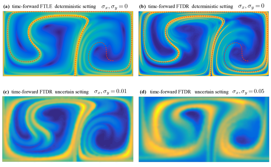
Figure 1. Time-forward FTLE (5.8) and kl-DR fields (4.18) in deterministic and stochastic flows generated by (6.7). The fields are computed over the interval $[t_{0},\,T]=[0,\,8]$ for a non-autonomous flows induced by (6.7) with parameters $\mathfrak{B}\,{=}\,1$, $\delta\,{=}\,0.25$ and $\Omega\,{=}\,2$. The top row shows the FTLE and kl-DR fields in a deterministic setting; the dashed-red line represents a stable flow-invariant manifold. The good qualitative agreement between agreement the two fields is in line with the bounds (5.9) and (5.12). The bottom row shows kl-DR fields in uncertain velocity field in (6.7) for two different values of noise amplitude. The ridges (yellow) in both types of fields indicate regions of maximal Lagrangian expansion.

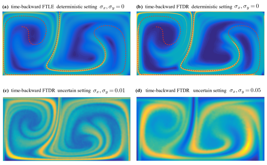
Figure 2. Time-backward FTLE (5.8) and kl-DR fields (4.19) in deterministic and stochastic flows generated by the dynamics (6.7); the fields are computed over the interval $[t_{0},\,T]=[-8,\,0]$. The dashed-red line represents the unstable flow-invariant manifold. See figure 1 for more details.

The fields of finite-time divergence rates ($\varphi$-DRF in (4.18)) are needed in the computational approach to quantification and mitigation of uncertainty in Lagrangian predictions through the bounds (2.3)-(2.4). The analytical properties of $\varphi$-DRF’s were established in Theorem 4.12 of §4.3 and the set-oriented reformulation, which is amenable to numerical approximations, was outlined in earlier in this section (Lemma 6.1 and Definition 6.2), while the links to Lyapunov exponent fields were established in §5.1. It is worth reiterating that $\varphi$-DRF’s are well defined for a general nonlinear stochastic flow and no linearisation in the computations is required.

Here, we illustrate our probabilistic approach for determining the fields of path-based expansion rates via kl-DRF (i.e., divergence rate field based on the KL-divergence) on a number of low-dimensional examples, and we compare them with the corresponding FTLE fields. The relationship between kl-DR and FTLE fields, while interesting, is at best of secondary importance from the perspective of Lagrangian Uncertainty Quantification (LUQ) in reduced models [17]. However, the abundance and popularity of approaches based on finite-time Lyapunov exponents in the Lagrangian transport analysis merits a comparison. At the same time, it is worth stressing that the bounds (2.3)-(2.4) utilised in [17] generally rely on the global structure of the expansion/divergence rates (expressed via $\varphi$-DRF’s, not FTLE’s) and not on a detailed structure of their local maximisers and minimisers. Hence, extensions of Lyapunov exponent-based approaches to the stochastic case (e.g., via (5.8)) are not useful in our subsequent applications to LUQ due to the form of the bounds (2.3)-(2.4). Moreover, the $\varphi$-DR fields, including kl-DRF and their set-oriented approximations (6.6), rely on the evolution of the underlying time-marginal probability measures induced by an arbitrary nonlinear deterministic or stochastic flow.

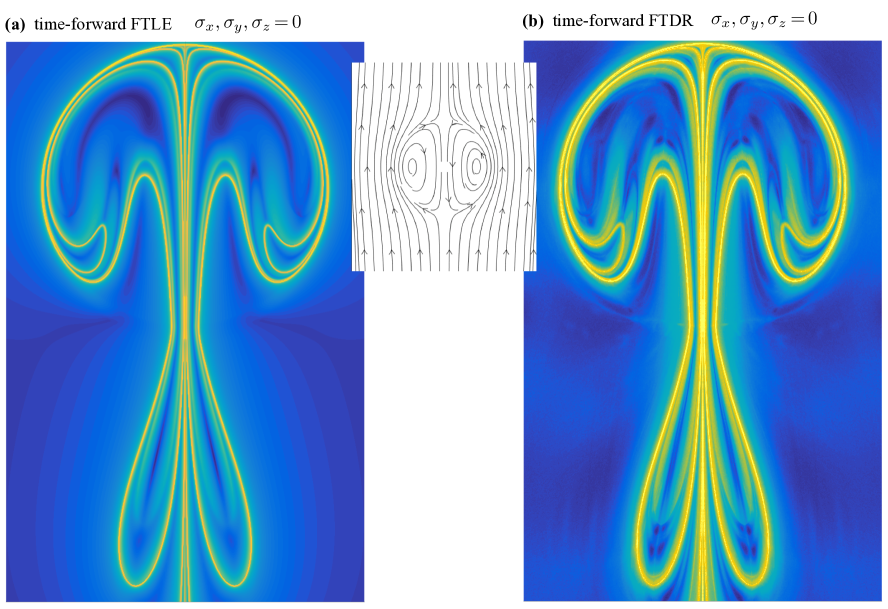
Figure 3. Time-forward FTLE (5.8) and kl-DR fields (4.18) in a deterministic flow generated by (6.8) for $\sigma_{x}\,{=}\,\sigma_{y}\,{=}\,\sigma_{z}\,{=}\,0$. The fields are computed over the interval $[t_{0},\,T]=[0,\,8]$ for a non-autonomous flow induced by (6.8). The ridges (yellow) in both types of maps indicate regions of maximal Lagrangian expansion; time-backward fields are shown in figure 5. See also figure 1.

To illustrate our methodology we consider two toy examples. First, we consider the following 2D system SDEs, which represents a periodically driven ‘double gyre’ flow with additive stochastic noise

$$\left.\begin{array}[]{l}dx=-\pi\mathfrak{B}\sin(\pi f(t,x))\cos(\pi y)+\sigma_{x}dW^{x}_{t},\\[8.5359pt] dy=\pi\mathfrak{B}\cos(\pi f(t,x))\sin(\pi y)\partial_{x}f(t,x)+\sigma_{y}dW^{y}_{t},\end{array}\right\}$$ (6.7)

where $f(x,t)=\delta\sin(\Omega t)x^{2}+(1-2\delta\sin(\Omega t))x$; the dynamics is defined on a two-dimensional flat torus, where we take $\mathcal{M}:=[0,\,2]\times[0,\,1]$ with doubly-periodic boundary conditions.

For $\sigma_{x}\,{=}\,\sigma_{y}\,{=}\,0$ the dynamics (6.7) reduces to the well-known benchmark for studying Lagrangian transport; note that in the deterministic case the boundary of $\mathcal{M}$ is invariant under the induced flow. When $\delta\,{=}\,0$ in $f(t,x)$ the system (6.7) is autonomous and it has two hyperbolic fixed points on the boundary at $(1,0)$ and $(0,1)$ whose stable and unstable manifolds partition $\mathcal{M}$. For $0<\epsilon\ll 1$ (i.e., the non-autonomous case) these two fixed points morph into non-trivial hyperbolic trajectories which are confined to the boundary of $\mathcal{M}$ which move along $[1,x]$ and $[0,x]$, $x\in[0,\;2]$ with a period $2\pi/\Omega$. For $t=0$ these hyperbolic trajectories are in the same position as the fixed points in the autonomous case, whereas for $t=2\pi/\Omega$ these trajectories are at their extreme locations. The stable and unstable manifolds of these two hyperbolic trajectories form a heteroclinic tangle which has been the focus of many computational studies (e.g., [18, 67, 37, 53]). In the presence of stochastic noise in (6.7) the above deterministic picture no longer applies but one is still interested in the spatial structure of local expansion rates.

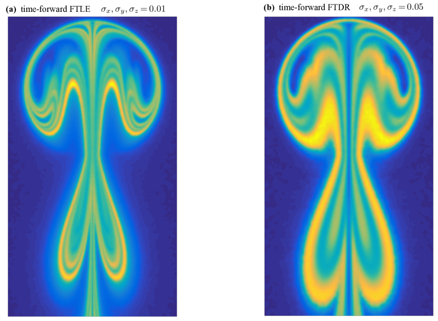
Figure 4. Time-forward FTLE (5.8) and kl-DR fields (4.18) in a stochastic flow generated by (6.8) for two different amplitudes of additive noise. The fields are computed over the interval $[t_{0},\,T]=[0,\,8]$ for a non-autonomous flow induced by (6.8). The ridges (yellow) indicate regions of maximal Lagrangian expansion. Compare these fields with those for the deterministic dynamics of (6.8) shown in figure 3.

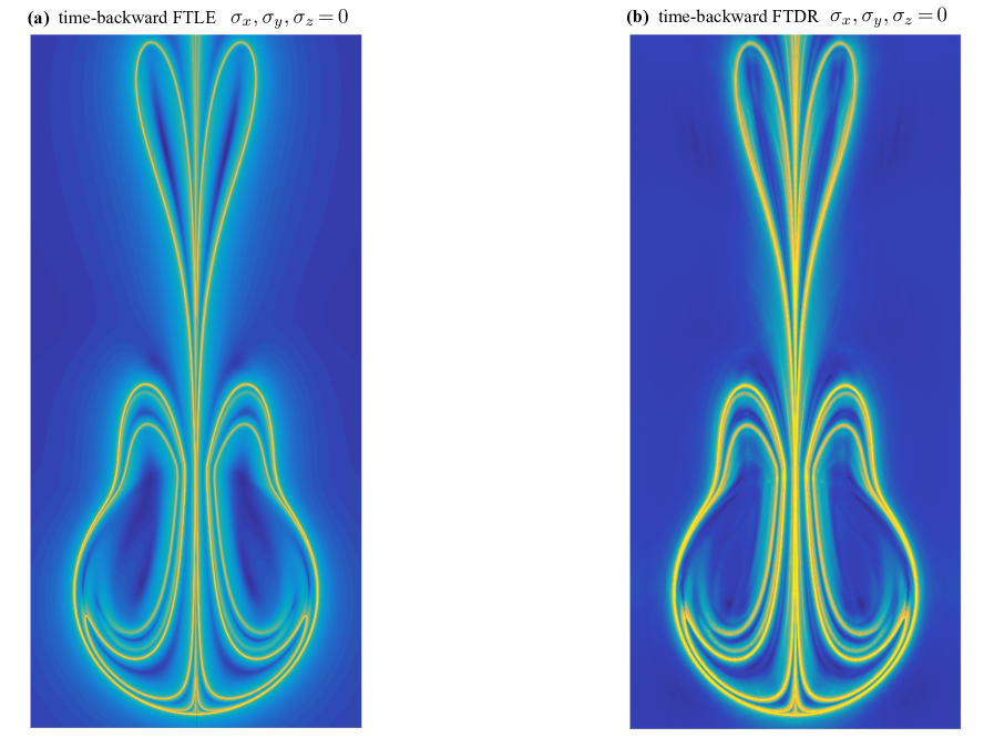
Figure 5. Time-backward FTLE (5.8) and kl-DR fields (4.19) and (4.4) in a deterministic flow generated by (6.8) for $\sigma_{x}\,{=}\,\sigma_{y}\,{=}\,\sigma_{z}\,{=}\,0$. The fields are computed over the interval $[t_{0},\,T]=[-8,\,0]$ for a non-autonomous flow induced by (6.8). The ridges (yellow) in both types of maps indicate regions of maximal Lagrangian expansion (backwards in time). See also figure 3 for the associated time-forward FDTR fields.

In Figures 1 and 2 we compare the numerical approximations of kl-DRF ((4.18) and (6.6)) and the average FTLE fields (5.8); where appropriate, we also determine the geometry of stable and unstable manifolds of the two hyperbolic trajectories confined to the top and bottom boundary of $\mathcal{M}$ based on methods described in [58, 59, 18]. We fix parameter values in (6.7) as $\mathfrak{B}\,{=}\,1$, $\delta\,{=}\,0.25$ and $\Omega\,{=}\,2$ and the results show FTLE and FTDR fields computed over the time interval $[t_{0},\;T]=[0,\,8]$ for the forward fields, and over $[t_{0},\;T]=[-8,\,0]$ for the backward fields. To create a numerical approximation of the transfer operators $(\mathcal{P}^{\Phi^{x}*}_{t,t_{0}})_{t\in\mathcal{I}}$, the domain $\mathcal{M}$ is partitioned into $N=1000^{2}$ boxes. The transition matrix $\tilde{\mathcal{P}}_{t,t_{0}}^{n}$ in (6.6) is estimated by numerically integrating the system with respect to $N^{2}=1000^{2}$ inner grid points per box using the 4th-order Runge-Kutta scheme in the deterministic case or the Euler-Maruyama scheme in the stochastic case (with time step chosen to guarantee numerical convergence and desired accuracy).

As a final example, consider the dynamical system associated with the well-known solution of the Euler’s equation of an inviscid incompressible fluid flow given by the Hill’s spherical vortex (e.g., [10]). The SDE associated with stochastically perturbed Hill’s vortex in Cartesian coordinates are

$$\left.\begin{array}[]{l}dx=\big{(}u_{r}(t)\sin\Theta+u_{\Theta}(t)\cos\Theta\big{)}\cos\Phi dx+\sigma_{x}dW_{t}^{x},\\[5.69046pt] dy=\big{(}u_{r}(t)\sin\Theta+u_{\Theta}(t)\cos\Theta\big{)}\sin\Phi dt+\sigma_{y}dW_{t}^{y},\\[5.69046pt] dz=\big{(}u_{r}(t)\cos\Theta-u_{\Theta}(t)\sin\Theta\big{)}dt+\sigma_{z}dW_{t}^{z},\end{array}\right\}$$ (6.8)

where $r=\sqrt{x^{2}+y^{2}+z^{2}}$, $\Theta=\textrm{acos(z/r)}$, $\Phi=\textrm{acos}(x/\sqrt{x^{2}+y^{2}})$. Assuming that $a>0$ denotes the radius of the vortex, the velocity components in the spherical coordinates are

$$u_{r}(t)=\begin{cases}\hskip 14.22636ptU\big{(}1-a^{3}(t)/r^{3}\big{)}\cos\Theta&\textrm{if}\quad r\geqslant a,\\[5.69046pt] -\textstyle{\frac{3}{2}}U\big{(}1-r^{2}/a^{2}(t)\big{)}\cos\Theta&\textrm{if}\quad r<a,\end{cases}$$

$$u_{\Theta}(t)=\begin{cases}-U\big{(}1+a(t)^{3}/(2r^{3})\big{)}\sin\Theta&\textrm{if}\quad r\geqslant a,\\[5.69046pt] \textstyle{\frac{3}{2}}U\big{(}1-2r^{2}/a^{2}(t)\big{)}\sin\Theta&\textrm{if}\quad r<a,\end{cases}$$

where we set $U=2$. In the deterministic, autonomous case the steady Hill’s vortex flow has two hyperbolic fixed points

$$h_{1}=(0,0,-a)^{T},\quad h_{2}=(0,0,a)^{T},$$

which are located on the (flow-invariant) axis of symmetry $\boldsymbol{e}_{z}$ of the vortex. The fixed point $h_{1}$ has a two-dimensional unstable manifold in $\mathbb{R}^{3}$ and the fixed point $h_{2}$ has a two-dimensional stable manifold in $\mathbb{R}^{3}$ ([18]). We consider a non-autonomous version of the dynamics (6.8) and set

$$a(t)=2+0.12\sin(2.2t).$$

This time-dependence does not break the axial symmetry of the dynamics and, consequently, any plane containing $\boldsymbol{e}_{z}$ is invariant under the (deterministic) flow. This, in turn, implies that the stable and unstable manifolds of hyperbolic trajectories, $\gamma_{h_{1}}(t),\gamma_{h_{2}}(t)$, confined to the axis of symmetry are foliated by planes containing $\boldsymbol{e}_{z}$ (i.e., at any fixed $t$, the stable and unstable manifolds of $\gamma_{h_{1}}(t),\gamma_{h_{2}}(t)$ intersect any invariant plane along a 1D curve). These trajectories can be computed using the algorithms of [47, 48]. Their stable and unstable manifolds are computed as in the previous examples using techniques described in [58, 59, 18]. In Figures 3–5 we compare numerical approximations of kl-DRF fields and FTLE fields associated with the dynamics (6.8); figures 3 and 5 correspond to the deterministic dynamics in (6.8) with $\sigma_{x}\,{=}\,\sigma_{y}\,{=}\,\sigma_{z}\,{=}\,0$, and figure 4 illustrates the structure of FTDR fields in the stochastic case.

For deterministic version of the dynamics in (6.7) and (6.8) both kl-DRF and FTLE fields match well the location of the stable and unstable manifolds of the two hyperbolic trajectories (see figures 1(a,b), 2(a,b), 3, and 5) which is in line with the bounds (5.9) and (5.12). Remnants of the deterministic Lagrangian structures persist for small values of the noise amplitude but they gradually degrade with increasing amplitude of the stochastic noise (Figures 1(c,d), 2(c,d), 4), and/or when the fields are computed over increasingly long time intervals. This behaviour is to be expected and it does invalidate the bounds (2.4) not their utility for tuning reduced models at finite times. For example, for ergodic dynamics the support of the measures $\mathcal{P}_{t,t_{0}}^{\Phi^{x}*}\tilde{\mu}^{x,\varepsilon}_{t_{0}}$ increases all of $\mathcal{M}$ as $t\,{\rightarrow}\,\infty$. Consequently, the KL-divergence $\mathcal{D}_{\textsc{kl}}(\mathcal{P}_{t,t_{0}}^{\Phi^{x}*}\tilde{\mu}^{x,\varepsilon}_{t_{0}}\|\tilde{\mu}^{x,\varepsilon}_{t_{0}})$ approaches its asymptotic value $\mathcal{D}_{\textsc{kl}}(\bar{\mu}\|\tilde{\mu}^{x,\varepsilon}_{t_{0}})$ for any $x\in\mathcal{M}$ so that the corresponding expansion rate field $\mathcal{R}^{\Phi}_{\textsc{kl},\varepsilon}(x;t_{0},t)$ in (4.18) decays to zero as $t\rightarrow\infty$ after reaching some intermediate maximum value.

More advanced approaches to estimating the $\varphi$-DR fields (utilising adaptive techniques akin to those [37, 38, 33] and for approximating the probability measures in higher dimension as in [23, 24]) and utilisation of the bound (2.4) as a loss function in statistical and machine/deep learning of coarse-grained models are postponed to a subsequent publication devoted to applications.

7. Conclusions and future work

We developed a new probabilistic framework for characterising nonlinear trajectorial expansion rates in non-autonomous stochastic dynamical systems that can be defined over a finite time interval and used for the subsequent uncertainty quantification in Lagrangian (trajectory-based) predictions. These nonlinear expansion rates are quantified via the family of $\varphi$-divergences between probability measures induced by the law of the stochastic flow associated with the underlying dynamics. The stochastic flow formulation elucidates connections between the path space measures, the evolution of their time-marginal probability measures, and path-based local stretching rates. We constructed scalar fields of local finite-time divergence/expansion rates termed ($\varphi$-DRF), showed their existence for general stochastic flows, continuity in time and the spatial parameter, and we derived a hierarchy of bounds that are important in practical uncertainty quantification tasks using $\varphi$-DRF. These fields can be subsequently combined with information inequalities (2.3)-(2.4) derived in [17] to mitigate the uncertainty in path-based observables estimated from approximations of the true dynamics in a way that is amenable to algorithmic implementations, and it can be utilised in information-geometric analysis of statistical estimation and inference on families of models, as well as in machine/deep learning approaches to the identification of accurate models for Lagrangian predictions.

Moreover, for the particular case of the Kullback-Leibler divergence the corresponding expansion rates were linked to the Lyapunov exponents for probability measures, as well as the finite-time Lyapunov exponents for path-based observables; the latter are commonly used for estimating expansion rates in Lagrangian transport considerations and our results should be relevant when considering some of its aspects in a more general probabilistic setting.

This work was motivated by the desire to quantify the evolution of uncertainty and improving path-based/Lagrangian predictions in complex dynamical systems based on simplified, data-driven models, especially in geophysical applications. A follow-up study combining the above results with the framework for Lagrangian uncertainty quantification [17], as outlined in §2.2, will focus on applications of these tools for deriving optimised models for accurate Lagrangian predictions over different time-horizons, and on understanding the role of both the Eulerian characteristics of the underlying dynamics and the dominant Lagrangian structures on the skill of path-based predictions in applications. In particular, the use of the bound (2.4) as a loss function in machine/deep learning of coarse-grained models is of special interest and will be discussed in a separate publication.

Acknowledgements. M.B. acknowledges the support of Office of Naval Research grant ONR N00014-15-1-2351. K.U. is funded as a postdoctoral researcher on the above grant.

Appendix A Further proofs

A.1. Proof of Proposition 3.5

The procedure is similar to derivations in [52, §4.3]. Densities of $\Pi_{t,s}$ and $\check{\Pi}_{t,s}$ w.r.t. $\mu_{s}\in\mathord{\raisebox{-0.95001pt}{\scaleobj{.86}{\includegraphics[width=10.00002pt]{PP.pdf}}}}\hskip 0.56917pt(\mathcal{M})$ are related by the stochastic flow of diffeomoprphisms $\big{\{}\phi_{s,t}\big{\}}_{s,t\in\mathcal{I}}$. In order to see this, recall the change-of-variable formula

$$\int_{\phi_{t,s}(A,\omega)}f(y)m_{d}(dy)=\int_{A}f(\phi_{t,s}(x,\omega))\big{|}\!\det D\phi_{t,s}(x,\omega)\big{|}m_{d}(dx)\quad\mathbb{P}\textrm{-a.s.},\quad f_{\infty}\in\mathcal{C}(\mathcal{M}).$$ (A.1)

If $\mu_{s}$ has a strictly positive density $\rho_{s}(x)=d\mu_{s}/dm_{d}>0$, then by (A.1) the measure $\check{\Pi}_{t,s}$ satisfies

$$\check{\Pi}_{t,s}(A,\omega)=\mu_{s}(\phi_{t,s}(A,\omega)) =\int_{A}\rho_{s}(\phi_{t,s}(x,\omega))\rho_{s}^{-1}(x)\big{|}\!\det D\phi_{t,s}(x,\omega)\big{|}\mu_{s}(dx),\quad\forall A\in\mathcal{B}(\mathcal{M}),$$

where $D\phi_{t,s}(x,\omega)$ denotes the Jacobian matrix of $\phi_{t,s}(x,\omega)$ and $|\det D\phi_{t,s}(x,\omega)|\neq 0\;\;\mathbb{P}\textrm{-a.s.,}$ and it follows that

$$\alpha_{t,s}(x,\omega):=\frac{d\check{\Pi}_{t,s}}{d\mu_{s}}=\rho^{-1}_{s}(x)\rho_{s}(\phi_{t,s}(x,\omega))\big{|}\!\det D\phi_{t,s}(x,\omega)\big{|},$$ (A.2)

is the Radon-Nikodym derivative of the probability measure $\check{\Pi}_{t,s}$ with respect to $\mu_{s}$. In fact, if $\rho_{s}\in\mathcal{C}^{3}(\mathcal{M};\mathbb{R}^{+})\cap L^{1}(\mathcal{M},\mathbb{R}^{+})$, then $\alpha_{t,s}(x)$ admits the integral representation [52, Lemma 4.3.1]

$$\alpha_{t,s}(x,\omega) =\exp\bigg{\{}\int_{s}^{t}\rho_{s}^{-1}(\phi_{s,\xi}(x,\omega))\,\text{div}(\rho_{s}b)(\xi,\phi_{\xi,s}(x,\omega))d\xi$$

$$\hskip 56.9055pt+\int_{s}^{t}\sum_{k=1}^{d}\rho_{s}^{-1}(\phi_{s,\xi}(x,\omega))\,\text{div}(\rho_{s}\sigma_{k})(\xi,\phi_{s,\xi}(x,\omega))\circ dW_{\xi}^{k}(\omega)\bigg{\}},$$ (A.3)

where $\sigma_{k}$ denote the columns of $\sigma$ in (2.1). Similarly, the random measure $\Pi_{t,s}$ is given by

$$\Pi_{t,s}(A,\omega)=\mu_{s}(\phi_{t,s}^{-1}(A,\omega)) =\int_{A}\frac{\rho_{s}(\phi_{t,s}^{-1}(x,\omega))}{|\!\det D\phi_{t,s}(\phi_{t,s}^{-1}(x,\omega),\omega)|\rho_{s}(x)}\mu_{s}(dx),$$

so that the Radon-Nikodym derivative of $\Pi_{t,s}$ with respect to $\mu_{s}$ is given by

$$\pi_{t,s}(x,\omega):=\frac{d\Pi_{t,s}}{d\mu}=\rho_{s}^{-1}(x)\rho_{s}(\phi_{t,s}^{-1}(x,\omega))\big{|}\!\det D\phi_{t,s}(\phi_{t,s}^{-1}(x,\omega),\omega)\big{|}^{-1}.$$ (A.4)

The two densities in (A.2) and (A.4) are related by

$$\pi_{t,s}^{-1}(x,\omega)=\alpha_{t,s}(\phi_{t,s}^{-1}(x,\omega),\omega);$$ (A.5)

the above relationship is crucial as it is generally not possible to write the stochastic integral governing $\pi_{t,s}$ which we need in the derivations of §4.

A.2. Proof of Theorem 3.6

We present the proof of the second part of the theorem to make this article self-contained (see [52, 55] for more details). Under the imposed regularity assumptions on the coefficients of (2.1), the maps $\phi_{t_{0},t}(\,\cdot\,,\omega)$ and $\phi_{t_{0},t}^{-1}(\,\cdot\,,\omega)$ are $\mathcal{C}^{1}$- diffeomorphisms (e.g., [51, 52]) and there exist $K_{\omega}\in\cap_{p>1}L^{p}(\Omega)$ and $\alpha>1$ such that

$$|\phi_{t_{0},t}^{-1}(x,\omega)|\leqslant K_{\omega}(1+|x|^{\alpha}),\quad\text{for all $(t_{0},t,x)$}\in\mathcal{I}\times\mathcal{I}\times\mathcal{M}.$$ (A.6)

Let $B_{r}\subset\mathcal{M}\subseteq\mathbb{R}^{d}$ be a ball of radius $r>0$. The spatial estimate (A.6) implies that

$$\phi_{t_{0},t}^{-1}(B_{r},\omega)\subset B_{K_{\omega}(1+r^{\alpha})},$$

and, due to the monotone property of the finite positive measure $\mu_{t_{0}},$ we have

$$\mu_{t_{0}}(\phi_{t_{0},t}^{-1}(B_{r},\omega))\leqslant\mu_{t_{0}}(B_{K_{\omega}|1+r^{\alpha}|})=\!\!\int_{B_{K_{\omega}|1+r^{\alpha}|}}\rho_{t_{0}}(x)m_{d}(dx)\leqslant\!\!\sup_{x\in B_{K_{\omega}|1+r^{\alpha}|}}\!\!\!\!\big{\{}\rho_{t_{0}}(x)\big{\}}V_{d}(1)K_{\omega}^{d}|1+r^{\alpha}|^{d},$$

where $V_{d}(1)$ is the volume of the unit ball in $\mathbb{R}^{d}$. Therefore,

$$\mathbb{E}\Big{(}\sup_{t\in\mathcal{I}}\,\big{[}\mu_{t_{0}}(\phi_{t_{0},t}^{-1}(B_{r},\omega))\big{]}^{p}\Big{)}\leqslant V_{d}(1)^{p}(1+r^{\alpha})^{pd}\,\mathbb{E}\big{[}M^{p}K_{\omega}^{pd}\big{]}<\infty,\quad\forall\;p>1,$$ (A.7)

where $M:=\sup\{\rho_{t_{0}}(x):x\in B_{K_{\omega}|1+r^{\alpha}|}\}<\infty$. This procedure can be extended to a set of the form $\bigcup_{x\in S}B_{r(x)}(x)$ for some countable subset of $S\subset\mathcal{M}$ provided that the density of the initial measure is sufficiently smooth and strictly positive (see, e.g., [55] for details). Thus, by the covering lemma, the above construction can be extended to any Borel measurable subset $A\in\mathcal{B}(\mathcal{M})$ and we have that $\mu_{t}\ll m_{d},\;\mathbb{P}\,\textrm{-a.s.}$  for  $t\in\mathcal{I}.$

Finally, in order to derive (3.8), note that for any $f\in\mathcal{C}_{c}^{\infty}(\mathcal{M}),$

$$\int_{\mathcal{M}}f(\phi_{t_{0},t}(x,\omega))\mu_{t_{0}}(dx)=\int_{\mathcal{M}}f(y)\frac{d(\mu_{t_{0}}\circ\phi_{t_{0},t}^{-1})(y)}{d\mu_{t_{0}}}\mu_{t_{0}}(dy)=\int_{\mathcal{M}}f(y)\pi_{t_{0},t}(y,\omega)\mu_{t_{0}}(dy).$$ (A.8)

On the other hand, we have

$$\int_{\mathcal{M}}f(x)\mu_{t}(dx)=\int_{\mathcal{M}}\mathbb{E}\big{[}f\big{(}\phi_{t_{0},t}(x,\,\cdot\,)\big{)}\big{]}\mu_{t_{0}}(dx).$$ (A.9)

Combining (A.8) and (A.9) leads to

$$\int_{\mathcal{M}}f(x)\mu_{t}(dx)=\int_{\mathcal{M}}f(x)\mathbb{E}\big{[}\pi_{t_{0},t}(x,\,\cdot\,)\big{]}\rho_{t_{0}}(x)m_{d}(dx),\quad f\in\mathcal{C}_{c}^{\infty}(\mathcal{M}),$$

which gives

$$\hskip 113.81102pt\mu_{t}(dx)=\rho_{t_{0}}(x)\mathbb{E}\big{[}\pi_{t_{0},t}(x,\,\cdot\,)\big{]}m_{d}(dx),\quad t\in\mathcal{I}.\hskip 99.58464pt\qed$$

A.3. Comments on Theorem 3.10

The imposed regularity of the coefficients $(\mathring{b},\sigma)$ guarantees the existence of global strong solutions of the SDE (2.1) and the existence of the extremal solution of the martingale problem associated with $\mathcal{L}_{t}$ for $m_{d}$ - a.e. initial condition $x\in\mathcal{M}$, leading to the existence and uniqueness of the weak$-^{*}$ solution of the forward Kolmogorov equation (3.15); e.g., [36, 14, 69]. Then, the existence of the Lebesgue density $(\rho_{t})_{t\in\mathcal{I}}$ solving (3.18) when $\mu_{t_{0}}\ll m_{d}$, and the representation (3.8) follows from the existence of a stochastic flow of solutions of (2.1) and Theorem 3.6. If $\rho_{t_{0}}=d\mu_{t_{0}}/dm_{d}\in\mathcal{C}^{2}_{\infty}(\mathcal{M};\mathbb{R}^{+})\cap L^{1}(\mathcal{M};\mathbb{R}^{+})$, the existence of unique solutions $\rho_{t}\in\mathcal{C}^{2}_{\infty}(\mathcal{M};\mathbb{R}^{+})\cap L^{1}(\mathcal{M};\mathbb{R}^{+})$, $t\in\mathcal{I}$, follows from the Feller property of transition evolutions $(\mathcal{P}_{s,t})_{t\geqslant s}$ induced by the stochastic flow and Itô formula. Finally, the last statement follows from the smoothing property of transition evolutions in such a setup.

A.4. Proof of Proposition 3.13

Given the assumptions of the proposition, the derivative flow $\big{\{}D\phi_{t_{0},t}(\,\cdot\,,\,\cdot\,)\big{\}}_{t\in\mathcal{I}}$ exists and is bounded from below due to Theorem 3.11, and the map $y\mapsto\Phi^{x}_{t,t_{0}}(y,\omega)$ in (3.20) is a $\mathcal{C}^{1}$ -diffeomprphism. Differentiating $\Phi^{x}_{t_{0},t}(y,\omega)$ with respect to $y\in\mathcal{M}$ at $y=0$, (see, e.g., [52, Theorem 3.3.4]) yields for all $t\in\mathcal{I}$

$$D\Phi^{x}_{t_{0},t}(\omega)=D\phi_{t_{0},t}(x,\omega)\quad\mathbb{P}\,\textrm{-\,a.s.}$$ (A.10)

The relationship in (A.10) implies, in particular, that the solutions $y_{t}=D\phi_{t_{0},t}(x,\omega)y$ associated with (3.11) coincide $\mathbb{P}\,\textrm{-\,a.s.}$ with $y_{t}=D\Phi^{x}_{t,t_{0}}(\omega)y$ for $x,y\in\mathcal{M}$. Thus, if $D\phi_{t_{0},t}(x,\omega)$ is bounded away from zero for $t\in\mathcal{I}$, then $D\Phi_{t_{0},t}^{x}(\omega)^{-1}=D\phi_{t_{0},t}(x,\omega)^{-1}$ $\mathbb{P}$ - a.s. which implies that $D\Phi_{t_{0},t}^{x}(\omega)$ is nonsingular.

The rest of the proof exploits the Itô formula for continuous semimartingales obtained from the two-point motion $\big{\{}(\phi_{t,t_{0}}(x_{1},\omega),\phi_{t,t_{0}}(x_{2},\omega))\,{:}\;(x_{1},x_{2})\,{\in}\,\mathcal{M}\otimes\mathcal{M},\;t,t_{0}\,{\in}\,\mathcal{I}\big{\}}$.

First, consider a semi-martingale $V_{t}^{\scriptscriptstyle(N)}\!:\mathbb{R}^{Nd}\rightarrow\mathbb{R}^{Nd}$ with $V_{t,t_{0}}^{\scriptscriptstyle(N)}\!=(X^{x_{1}}_{t},\dots,X^{x_{N}}_{t})$, $(x_{1},\cdots x_{N})\in\otimes^{N}\mathcal{M}$, s.t. $X^{t_{0},x_{i}}_{t}$ solves (2.1) with the initial conditoin $x_{i}\in\mathcal{M}$. The continuous dependence the solutions $X^{t_{0},x_{i}}_{t}$ on the initial condition leads to the $N$-point motion generated by $\big{\{}(\phi_{t_{0},t}(x_{1},\omega),\cdots,\phi_{t_{0},t}(x_{N},\omega))\!\!:(x_{1},\cdots x_{N})\in\otimes^{N}\mathcal{M},\;t_{0},t\in\mathcal{I}\big{\}}$ which may be interpreted as a stochastic flow generated by ‘running’ (2.1) simultaneously from $N$ different initial conditions (see, e.g., [6, 52, 12] for details). The $N$-point motion of stochastic flows is a process on $\mathbb{R}^{Nd}$ with the generator $\mathcal{L}^{\scriptscriptstyle(N)}$ induced by (A.11) and transition evolutions $(\mathcal{P}^{\scriptscriptstyle(N)}_{t_{0},t})_{t\in\mathcal{I}}$ in the form (3.2) and generated by the transition kernel

$$P^{\scriptscriptstyle(N)}(t_{0},(x_{1},\dots,x_{N});t,E) :=\mathbb{P}\big{\{}\omega:(\phi_{t_{0},t}(x_{1},\omega),\dots,\phi_{t_{0},t}(x_{N},\omega)){\in}E\big{\}},\quad t_{0},t\in\mathcal{I},\;E\in\mathcal{B}({\otimes}^{\scriptscriptstyle N}\mathcal{M}).$$

Theorem A.1.

[Itô formula for continuous semimartingales [52]]. Let $V_{t,t_{0}}^{\scriptscriptstyle(N)}=(X^{x_{1}}_{t},\cdots,X_{t}^{x_{N}})$ be a continuous semi-martinagale with $X^{t_{0},x_{i}}_{t}=\phi_{t,t_{0}}(x_{i},\omega)$. If $g\in\mathcal{C}^{2}(\mathbb{R}^{Nd})$, then $g(V_{t}^{\scriptscriptstyle(N)})$ is a continuous semi-martingale which satisfies

$$g(V_{t,t_{0}}^{\scriptscriptstyle(N)})-g(V_{t_{0}}^{\scriptscriptstyle(N)})=\sum_{i=1}^{\scriptscriptstyle N}\int_{t_{0}}^{t}\partial_{x_{i}}g(V_{s,t_{0}}^{\scriptscriptstyle(N)})dX_{s}^{i}+\frac{1}{2}\sum_{i,j=1}^{\scriptscriptstyle N}\int_{t_{0}}^{t}\partial^{2}_{x_{i}x_{j}}g(V_{s,t_{0}}^{\scriptscriptstyle(N)})d\big{\langle}X_{s}^{i},X_{s}^{j}\big{\rangle}_{s}.$$ (A.11)

If $g\in\mathcal{C}^{3}(\mathbb{R}^{Nd})$, then we have

$$g(V_{t,t_{0}}^{\scriptscriptstyle(N)})-g(V_{t_{0}}^{\scriptscriptstyle(N)})={\sum_{i=1}^{\scriptscriptstyle N}}\int_{t_{0}}^{t}\partial_{x_{i}}g(V_{s,t_{0}}^{\scriptscriptstyle(N)})\circ dX_{s}^{i}.$$ (A.12)

Proof of Proposition 3.13: Consider the transition kernel for the two-point motion
$\big{\{}(\phi_{t_{0},t}(x_{1},\omega),\phi_{t_{0},t}(x_{2},\omega))\!:(x_{1},x_{2})\in\mathcal{M}\times\mathcal{M},\;t,t_{0}\in\mathcal{I}\big{\}}$ given by

$$P^{\scriptscriptstyle(2)}(t_{0},(x_{1},x_{2});t,E) :=\mathbb{P}\{\omega:(\phi_{t_{0},t}(x_{1},\omega),\phi_{t_{0},t}(x_{2},\omega))\in E\},\quad t_{0},t\in\mathcal{I},\quad E\in\mathcal{B}(\mathcal{M}{\times}\mathcal{M}),$$

and the corresponding transition evolution $\mathcal{P}_{t_{0},t}^{\scriptscriptstyle(2)}$ defined by

$$\mathcal{P}^{\scriptscriptstyle(2)}_{t,t_{0}}g(x_{1},x_{2}) :=\int_{\mathbb{R}^{2d}}g(u,z)P^{\scriptscriptstyle(2)}(t_{0},(x_{1},x_{2});t,du\otimes dz)=\mathbb{E}\big{[}g(\phi_{t_{0},t}(x_{1},\omega),\phi_{t_{0},t}(x_{2},\omega))\big{]},$$

for $g\in\mathbb{M}(\mathcal{M}\times\mathcal{M})$ and $\mu\otimes\nu\in\mathord{\raisebox{-0.95001pt}{\scaleobj{.86}{\includegraphics[width=10.00002pt]{PP.pdf}}}}\hskip 0.56917pt(\mathcal{M}\times\mathcal{M})$ with the dual

$$(\mathcal{P}^{\scriptscriptstyle(2)*}_{t,t_{0}}\mu\otimes\nu)(E)=\int_{\mathcal{M}\times\mathcal{M}}\!\!\!P^{\scriptscriptstyle(2)}(t_{0},(x_{1},x_{2});t,E)\mu\otimes\nu(dx_{1},dx_{2}),\quad t\geqslant t_{0},\quad E\in\mathcal{B}(\mathcal{M}{\times}\mathcal{M}),$$

where the extension of $g\in\mathbb{M}_{\infty}$ to $g\in\mathbb{M}$ is done in the standard way.

Now, let $X_{t}^{t_{0},x_{1}}(\omega)=\phi_{t_{0},t}(x_{1},\omega)$ and $X_{t}^{t_{0},x_{2}}(\omega)=\phi_{t_{0},t}(x_{2},\omega)$ be solutions of (2.1) starting from two initial conditions $x_{1},x_{2}\in\mathcal{M}$. Then, according to the Itô’s formula (A.12) with $g({x}_{1},x_{2})=x_{1}-x_{2}$, the process $V^{\scriptscriptstyle(2)}_{t,t_{0}}=\phi_{t_{0},t}(x_{1},\cdot)-\phi_{t_{0},t}(x_{2},\cdot)$ is a semimartingale and it can be represented as

$$V_{t,t_{0}}^{\scriptscriptstyle(2)}={x}_{1}{-}x_{2}+\!\!\int_{t_{0}}^{t}\!\Big{[}b(s,\phi_{s,t_{0}}(x_{1}))-b(s,\phi_{s,t_{0}}(x_{2}))\Big{]}ds+\!\!\int_{t_{0}}^{t}\!\Big{[}\sigma(s,\phi_{s,t_{0}}(x_{1}))-\sigma(s,\phi_{s,t_{0}}(x_{2}))\Big{]}{\circ}\,dW_{s}.$$ (A.13)

Next, for $g\in\mathcal{C}^{2}(\mathcal{M}\,{\times}\,\mathcal{M})$, define

$$\mathcal{P}^{\scriptscriptstyle(2)}_{t,t_{0}}\,g(x_{1}-x_{2}):=\mathbb{E}\Big{[}g\big{(}V_{t,t_{0}}^{\scriptscriptstyle(2)}\big{)}\Big{|}V_{t,t_{0}}^{\scriptscriptstyle(2)}=x_{1}-x_{2}\Big{]}=\int_{\mathcal{M}\times\mathcal{M}}g(y-u)P^{\scriptscriptstyle(2)}(t_{0},(x_{1},x_{2}));t,dy\otimes du).$$

Furthermore, the generator of the two-point motion $\{(\phi_{t_{0},t}(x,\omega),\phi_{t_{0},t}(y,\omega)):t_{0},t\in\mathcal{I},(x,y)\in\mathcal{M}\times\mathcal{M}\}$ is given by

$$\mathcal{L}^{\scriptscriptstyle(2)}_{t}:=\sum_{i=1}^{d}{b}_{i}(t,x)\partial_{x_{i}}+\sum_{i=1}^{d}{b}_{i}(t,y)\partial_{y_{i}}+{\textstyle\frac{1}{2}}\sum_{i,j=1}^{2d}\sum_{k=1}^{d}\sigma_{k,i}(t,x,y)\sigma_{k,j}(t,x,y)\partial^{2}_{x_{i}x_{k}},$$

where $\sigma_{k,i}(t,x,y):=\sigma_{ki}(t,x)$ and $\sigma_{k,i+d}(t,x,y):=\sigma_{kj}(t,y),$ $i=1,2,\cdots,d$. Finally, application of Itô’s formula (Theorem A.1) to the process $g\left(V^{\scriptscriptstyle(2)}_{t,t_{0}}(\omega)\right)=g\left(\phi_{t,t_{0}}(x_{1},\omega)-\phi_{t,t_{0}}(x_{2},\omega)\right),$ $t_{0},t\in\mathcal{I}$, for $g\in\mathcal{C}_{\infty}^{2}(\mathcal{M}\times\mathcal{M})$, gives a simplified form of the generator $\mathcal{L}_{t}^{\scriptscriptstyle(2)}$ as

$$\mathcal{L}^{\scriptscriptstyle(2)}_{t}g(x_{1}-x_{2}) =\left({b}(t,x_{1})-{b}(t,x_{2})\right)\partial_{x}\,g(x_{1}-x_{2})$$

$$\hskip 56.9055pt+{\textstyle\frac{1}{2}}\text{tr}\left(\big{[}\sigma(t,x_{1})-\sigma(t,x_{2})\big{]}^{T}\mathcal{H}_{g}(x_{1}-x_{2})\big{[}\sigma(t,x_{1})-\sigma(t,x_{2})\big{]}\right).$$

Setting $x_{1}=x+y$ and $x_{2}=x$ in the above two expressions for $\mathcal{P}^{\scriptscriptstyle(2)}_{t,t_{0}}$ and $\mathcal{L}^{\scriptscriptstyle(2)}_{t}$ yields, $\mathcal{P}^{\Phi^{x}}_{t,t_{0}}$ in (3.22) and $\mathcal{L}^{x}_{t}$ in (3.23). ∎

A.5. Proof of Lemma 4.5

Given the same assumptions as in Theorem 4.3 we have for $t,t_{0}\in\mathcal{I}$

$$\mathcal{D}_{\varphi}(\mu_{t}\|\mu_{t_{0}})= \int_{\mathcal{M}}\varphi\left(\rho_{t}(x)/\rho_{t_{0}}(x)\right)\rho_{t_{0}}(x)m_{d}(dx)$$

$$\underset{\textrm{Thm \ref{mut_rnd},\,\ref{FKPt1}}}{=}\int_{\mathcal{M}}\varphi\Big{(}\mathbb{E}[\pi_{t_{0},t}(x)]\Big{)}\rho_{t_{0}}(x)m_{d}(dx)$$

$$\underset{\text{Jensen's ineq.}}{\leqslant}\int_{\mathcal{M}}\mathbb{E}[\varphi\big{(}\pi_{t_{0},t}(x)\big{)}]\rho_{t_{0}}(x)m_{d}(dx)$$

$$\underset{\textrm{Thm \ref{al_pi}}}{=}\int_{\mathcal{M}}\mathbb{E}\Big{[}\varphi\Big{(}\alpha_{t_{0},t}^{-1}\big{(}\phi_{t_{0},t}^{-1}(x)\big{)}\Big{)}\Big{]}\rho_{t_{0}}(x)m_{d}(dx)$$

$$\underset{\text{Fubini's thm.}}{=}\mathbb{E}\bigg{[}\int_{\mathcal{M}}\varphi\Big{(}\alpha_{t_{0},t}^{-1}\big{(}\phi_{t_{0},t}^{-1}(x)\big{)}\Big{)}\rho_{t_{0}}(x)m_{d}(dx)\bigg{]}$$

$$=\mathbb{E}\bigg{[}\int_{\mathcal{M}}\varphi\big{(}\alpha_{t_{0},t}^{-1}(\xi)\big{)}\rho_{t_{0}}(\phi_{t_{0},t}(\xi))\big{|}\!\det D\phi_{t_{0},t}(\xi)\big{|}\rho_{t_{0}}^{-1}(\xi)\rho_{t_{0}}(\xi)m_{d}(d\xi)\bigg{]}$$

$$=\mathbb{E}\bigg{[}\int_{\mathcal{M}}\varphi\big{(}\alpha_{t,t_{0}}^{-1}(\xi)\big{)}\alpha_{t_{0},t}(\xi)\rho_{t_{0}}(\xi)m_{d}(d\xi)\bigg{]}=\int_{\mathcal{M}}\mathbb{E}\big{[}\varphi_{\ddagger}\big{(}\alpha_{t_{0},t}(\xi)\big{)}\big{]}\mu_{t_{0}}(d\xi),$$

where $\mathbb{E}[\pi_{t_{0},t}(x)]:=\int_{\Omega}\pi_{t_{0},t}(x,\omega)\mathbb{P}(d\omega)$, $\mathbb{E}[\alpha_{t_{0},t}(x)]:=\int_{\Omega}\alpha_{t_{0},t}(x,\omega)\mathbb{P}(d\omega)$, and similarly
$\mathbb{E}\big{[}\varphi\big{(}\alpha_{t_{0},t}^{-1}\big{(}\phi_{t_{0},t}^{-1}(x)\big{)}\big{)}\big{]}:=\int_{\Omega}\big{[}\varphi\big{(}\alpha_{t_{0},t}^{-1}\big{(}\phi_{t_{0},t}^{-1}(x,\omega),\omega\big{)}\big{)}\big{]}$ to simplify notation.

A.6. Proof of Theorem 4.6

First, note that for $\mu_{t_{0}}\in\mathord{\raisebox{-0.95001pt}{\scaleobj{.86}{\includegraphics[width=10.00002pt]{PP.pdf}}}}\hskip 0.56917pt(\mathcal{M})$ with strictly positive Lebesgue density $\rho_{t_{0}}>0$ the (random) density process $\{\alpha_{t_{0},t}(x,\omega)\!:\,t_{0},t\in\mathcal{I}\}$, $\alpha_{t_{0},t}=d\check{\Pi}_{t_{0},t}/d\mu_{t_{0}}$, given in (4.4) is a continuous semi-martingale w.r.t. the natural (complete, right-continuous) filtration $(\mathcal{F}_{t_{0}}^{\,t})_{t\in\mathcal{I}}$, since by Itô’s formula it satisfies (see also ([52, Corollary 4.3.5]))

$$\alpha_{t_{0},t}(x,\omega)=1+\int_{t_{0}}^{t}\alpha_{t_{0},s}(x,\omega)G(s,\phi_{t_{0},s}(x,\omega))dW_{s}+\int_{t_{0}}^{t}\alpha_{t_{0},s}(x,\omega)\frac{\check{\mathcal{L}}_{s}^{*}\rho_{t_{0}}(\phi_{t_{0},s}(x,\omega))}{\rho_{t_{0}}(\phi_{t_{0},s}(x,\omega))}ds.$$ (A.14)

Moreover, note that for any convex $\varphi(u)$, $u>0$, the function $\varphi_{\ddagger}(u)=u\varphi(u^{-1})$ is also convex and locally bounded. In what follows we consider functions $\varphi$ satisfying (4.1) so that $\varphi_{\ddagger}(1)=0$. Thus, by Itô-Tanaka-Meyer formula (e.g., [64]), we have for any $t\in\mathcal{I}$

$$\varphi_{\ddagger}(\alpha_{t_{0},t}) =\varphi_{\ddagger}(\alpha_{t_{0},t_{0}})+\int_{t_{0}}^{t}D^{-}\varphi_{\ddagger}(\alpha_{t_{0},s})d\alpha_{t_{0},s}$$

$$\hskip 56.9055pt+\frac{1}{2}\int_{(0,\infty)}L^{\ell}_{t}(\alpha)\varphi^{\prime\prime}_{\ddagger}(d\ell)+\sum_{t_{0}\leqslant s\leqslant t}\big{(}\Delta\varphi_{\ddagger}(\alpha_{t_{0},s})-\varphi^{\prime}_{\ddagger}(\alpha_{t_{0},s^{-}})\Delta\alpha_{t_{0},s}\big{)}$$

$$=\int_{t_{0}}^{t}D^{-}\varphi_{\ddagger}(\alpha_{t_{0},s})d\alpha_{t_{0},s}$$

$$\hskip 56.9055pt+\frac{1}{2}\int_{(0,\infty)}L^{\ell}_{t}(\alpha)\varphi^{\prime\prime}_{\ddagger}(d\ell)+\sum_{t_{0}\leqslant s\leqslant t}\Delta\varphi_{\ddagger}(\alpha_{t_{0},s}),$$ (A.15)

where $L^{\ell}_{t}(\alpha)$ is the local time of $\alpha_{t_{0},t}(x,\omega)$ at level $\ell\geqslant 0$ (e.g., [64]) given by

$$L_{t}^{\ell}(\alpha)=2\Big{[}(\alpha_{t,t_{0}}-\ell)_{+}-(\alpha_{t_{0},t_{0}}-\ell)_{+}-\int_{t_{0}}^{t}\mathbb{I}_{\{\alpha_{t_{0},s}>\ell\}}d\alpha_{t_{0},s}-\sum_{t_{0}\leqslant s\leqslant t}\Delta(\alpha_{t_{0},s}-\ell)_{+}\Big{]},$$

$\Delta(\,\cdot\,)$ denotes a pure jump of the argument and the left-sided derivative $D^{-}\varphi_{\ddagger}$ is bounded on $\mathcal{I}$ due to the convexity of $\varphi_{\ddagger}$ on $(0,\infty)$.

Taking the expectation of (A.6) conditioned on $\mathcal{F}_{t_{0}}^{t},$ we have that

$$\mathbb{E}\big{[}\varphi_{\ddagger}(\alpha_{t_{0},t})\big{]} =\sum_{t_{0}\leqslant s\leqslant t}\mathbb{E}\big{[}\Delta\varphi_{\ddagger}(\alpha_{t_{0},s})\big{]}+\mathbb{E}\left[\int_{t_{0}}^{t}D^{-}\varphi_{\ddagger}(\alpha_{t_{0},s})\alpha_{t_{0},s}\frac{\check{\mathcal{L}}_{s}^{*}\rho_{t_{0}}(\phi_{t_{0},s})}{\rho_{t_{0}}(\phi_{t_{0},s})}ds\right]$$

$$\qquad+\frac{1}{2}\mathbb{E}\bigg{[}\int_{(0,\infty)}L^{\ell}_{t}(\alpha)\varphi^{\prime\prime}_{\ddagger}(d\ell)\bigg{]},$$

which, combined with the inequality (4.10), leads to the first assertion

$$\mathcal{D}_{\varphi}(\mu_{t}||\mu_{t_{0}}) \leqslant\sum_{t_{0}\leqslant s\leqslant t}\mathbb{E}\big{[}\Delta\varphi_{\ddagger}(\alpha_{t_{0},s})\big{]}+\int_{\mathcal{M}}\mathbb{E}\left[\int_{t_{0}}^{t}D^{-}\varphi_{\ddagger}(\alpha_{t_{0},s})\alpha_{t_{0},s}\frac{\check{\mathcal{L}}_{s}^{*}\rho_{t_{0}}(\phi_{t_{0},s})}{\rho_{t_{0}}(\phi_{t_{0},s})}ds\right]d\mu_{t_{0}}$$

$$\qquad+\frac{1}{2}\int_{\mathcal{M}}\mathbb{E}\bigg{[}\int_{(0,\infty)}L^{\ell}_{t}(\alpha)\varphi^{\prime\prime}_{\ddagger}(d\ell)\bigg{]}d\mu_{t_{0}}.$$

Next, if $\varphi$ is twice continuously differentiable on $(0,\infty)$, we obtain

$$\hskip 56.9055pt\mathcal{D}_{\varphi}(\mu_{t}\|\mu_{t_{0}}) \leq\int_{\mathcal{M}}\mathbb{E}\left[\int_{t_{0}}^{t}\varphi^{\prime}_{\ddagger}(\alpha_{t_{0},s})\alpha_{t_{0},s}\frac{\check{\mathcal{L}}_{s}^{*}\rho_{t_{0}}(\phi_{t_{0},s})}{\rho_{t_{0}}(\phi_{t_{0},s})}ds\right]\mu_{t_{0}}(dx)$$

$$\qquad+\frac{1}{2}\int_{\mathcal{M}}\mathbb{E}\bigg{[}\int_{t_{0}}^{t}\varphi_{\ddagger}^{\prime\prime}(\alpha_{t_{0},s})d\langle\alpha_{t_{0},s}\rangle\bigg{]}\mu_{t_{0}}(dx)$$

$$=\int_{\mathcal{M}}\mathbb{E}\left[\int_{t_{0}}^{t}\varphi^{\prime}_{\ddagger}(\alpha_{t_{0},s})\alpha_{t_{0},s}\frac{\check{\mathcal{L}}_{s}^{*}\rho_{t_{0}}(\phi_{t_{0},s})}{\rho_{t_{0}}(\phi_{t_{0},s})}ds\right]\mu_{t_{0}}(dx)$$

$$\qquad+\frac{1}{2}\int_{\mathcal{M}}\mathbb{E}\bigg{[}\int_{t_{0}}^{t}\varphi_{\ddagger}^{\prime\prime}(\alpha_{t_{0},s})\alpha^{2}_{t_{0},s}G^{2}(s,\phi_{t_{0},s})ds\bigg{]}\mu_{t_{0}}(dx).\hskip 56.9055pt\qed$$

Glossary

Here, we list further definitions and notation which recurs throughout the paper.

(2) Probability spaces and function spaces

• Wiener space. We fix the probability space $(\Omega,\mathcal{F},\mathbb{P})$ as the Wiener space, i.e., $\Omega\simeq\mathcal{C}_{0}(\mathcal{I};\mathbb{R}^{m})$, $m\in\mathbb{N}$, $\mathcal{I}:=[t_{0},\,T\hskip 0.56917pt)\subset\mathbb{R}$, $T>0$, is a subspace of continuous functions $\mathcal{C}(\mathbb{R};\mathbb{R}^{m})$ which are zero at $t_{0}\in\mathcal{I}$. $\mathcal{F}$ is the Borel $\mathfrak{S}$-algebra generated by open subsets in the compact-open topology on $\Omega$ defined via

  $$\varrho(\omega,\hat{\omega})=\sum_{\ell=0}^{\infty}\frac{1}{2^{\ell}}\frac{\|\omega-\hat{\omega}\|_{\ell}}{1+\|\omega-\hat{\omega}\|_{\ell}},\qquad\|\omega-\hat{\omega}\|_{\ell}:=\sup_{t\in[-\ell,\,\ell\,]}|\omega(t)-\hat{\omega}(t)|,\quad\omega,\hat{\omega}\in\Omega,$$

  with $|{\,\cdot\,}|$ the Euclidean norm on $\mathbb{R}^{m}$. Finally, $\mathbb{P}$ is the Wiener measure on $\mathcal{F}$.

• $\mathcal{W}_{d}:=\mathcal{C}(\mathcal{I},\mathcal{M})$ is the path space defined over $\mathcal{M}$. The Borel $\mathfrak{S}$-algebra $\mathcal{B}(\mathcal{W}_{d})$ on $\mathcal{W}_{d}$ are defined analogously to those in the Wiener space.

• For $f\,{:}\;\mathcal{M}\rightarrow\mathbb{R}$, where $(\mathcal{M},\mathcal{B}(\mathcal{M}))$ is a Polish space equipped with a Borel $\mathfrak{S}$ - algebra, the following function spaces are relevant:

  • $\mathbb{M}_{\infty}(\mathcal{M})$ space of bounded Borel measurable functions $\mathbb{M}(\mathcal{M})$ on $\mathcal{M}$.

  • $\mathbb{M}^{+}(\mathcal{M})$ space of non-negative Borel measurable functions on $\mathcal{M}$.

  • $\mathcal{C}_{\infty}(\mathcal{M})$ space of bounded continuous functions on $\mathcal{M}$.

  • $\mathcal{C}^{l}(\mathcal{M})$, $l\geqslant 1$, space of $l$-times continuously differentiable functions on $\mathcal{M}$.

  • $\mathcal{C}^{k}_{\infty}(\mathcal{M})$, $l\geqslant 1$, functions in $\mathcal{C}^{l}(\mathcal{M})$ which are bounded with bounded derivatives up to order $l$ on $\mathcal{M}$.

  • $\mathcal{C}_{c}^{+}(\mathcal{M})$ space continuous non-negative functions on $\mathcal{M}$ with compact supports.

  • $\mathcal{C}_{c}^{\infty}(\mathcal{M})$ space of smooth functions on $\mathcal{M}$ with compact support.

• $\tilde{\mathcal{C}}^{l,\delta}(\mathcal{M})$, is the space of functions $f\,{:}\;\mathcal{M}\,{\rightarrow}\,\mathcal{M}$ with the countable family of semi-norms

  $$\tilde{\|}f\tilde{\|}_{l,\delta;N}:=\|f\|_{l;N}+\sum_{|\alpha|=l}\sup_{x,y\in\textsf{B}_{N}\!,\,x\neq y}\frac{|D^{\alpha}f(x)-D^{\alpha}f(y)|}{|x-y|^{\delta}}<\infty,\quad 0<\delta\leqslant 1,\;N_{1}\in\mathbb{N},\hskip 17.07182pt$$

  $$\tilde{\|}f\tilde{\|}_{l;N}:=\sup_{x\in\mathcal{M}}\frac{|\langle f(x),x\rangle|}{1+|x|^{2}}+\sum_{1\leqslant|\alpha|\leqslant l}\sup_{x\in\textsf{B}_{N}}|D^{\alpha}f(x)|,$$

  where $\textsf{B}_{N}:=\{x\in\mathcal{M}:|x|\leqslant N\}$, $\displaystyle D^{\alpha}f(x):=\frac{\partial^{|\alpha|}f}{(\partial x_{1})^{\alpha_{1}}\cdots(\partial x_{d})^{\alpha_{n}}},\;|\alpha|:=\sum_{i=1}^{n}\alpha_{i}$, $\alpha_{i}\in\mathbb{N}_{0}$, and  $D^{0}\equiv\textrm{Id}$.

• $\bar{\mathcal{C}}^{l,\delta}(\mathcal{M})$, is the space of functions $f\,{:}\;\mathcal{M}\,{\rightarrow}\,\mathcal{M}$ with the countable family of semi-norms

  $$\tilde{\|}f\tilde{\|}_{l,\delta;N}:=\|f\|_{l;N}+\sum_{|\alpha|=l}\sup_{x,y\in\textsf{B}_{N}\!,\,x\neq y}\frac{|D^{\alpha}f(x)-D^{\alpha}f(y)|}{|x-y|^{\delta}}<\infty,\quad 0<\delta\leqslant 1,\;N_{1}\in\mathbb{N},\hskip 17.07182pt$$

  $$\tilde{\|}f\tilde{\|}_{l;N}:=\sup_{x\in\mathcal{M}}\frac{|f(x)|}{1+|x|}+\sum_{1\leqslant|\alpha|\leqslant l}\sup_{x\in\mathcal{M}}|D^{\alpha}f(x)|,$$

• $\mathcal{C}\big{(}\mathcal{I};\bar{\mathcal{C}}^{l,\delta}(\mathcal{M})\big{)}$, $\mathcal{I}\subseteq\mathbb{R}$, is the set of all continuous fields $f\,{:}\;\mathbb{R}\times\mathcal{M}\rightarrow\mathcal{M}$ such that $f(t,\,\cdot\,)\in\bar{\mathcal{C}}^{l,\delta}(\mathcal{M})$.

(3) Frequently used notation

• $\mathord{\raisebox{-0.85501pt}{\scaleobj{.86}{\includegraphics[width=9.00002pt]{PP.pdf}}}}\hskip 0.56917pt(\mathcal{M})$ is a set of all Borel probability measures on $\mathcal{M}$.

• $\mathcal{D}_{\varphi}\big{(}\mu\|\nu\big{)}$ is a $\varphi$-divergence between measures in $\mathord{\raisebox{-0.85501pt}{\scaleobj{.86}{\includegraphics[width=9.00002pt]{PP.pdf}}}}\hskip 0.56917pt(\mathcal{M})$; $\varphi$ is a strictly convex function (see (4.2)).

• $\mathcal{D}_{\varphi}^{t_{0},t}\big{(}\mu\|\nu\big{)}=\scaleobj{.9}{|t-t_{0}|^{-1}}\hskip 0.11374pt\mathcal{D}_{\varphi}^{t_{0},t}\big{(}\mu\|\nu\big{)}$ is a $\varphi$-divergence rate between measures in $\mathord{\raisebox{-0.85501pt}{\scaleobj{.86}{\includegraphics[width=9.00002pt]{PP.pdf}}}}\hskip 0.56917pt(\mathcal{M})$.

• $\big{\{}\phi_{s,t}(\,\cdot\,,\omega)\,{:}\;s,t\in\mathcal{I}\big{\}}$, $\omega\in\Omega$, denotes a stochastic flow on $\mathcal{M}$ (usually, but not exclusively) generated by the SDE (2.1); see §3. $\{\Phi^{x}_{t_{0},t}\}_{t\in\mathcal{I}}$, $\Phi^{x}_{t_{0},t}(y,\omega)=\phi_{t_{0},t}(x+y,\omega)-\phi_{t_{0},t}(x,\omega)$, is the two-point motion associated with $\{\phi^{x}_{t_{0},t}\}_{t\in\mathcal{I}}$.

• $(\mathring{b},\sigma)$ are the drift and diffusion coefficients of the SDE (2.1). $\{\sigma_{k}\}_{k=1}^{m}$ stand for columns of the matrix field $\sigma$ with coefficients $\sigma_{ik}$.

• ${b}_{i}(t,x)\,{:=}\,\mathring{b}_{i}(t,x)\,{+}\,c_{i}(t,x)$, $c_{i}(t,x):=\frac{1}{2}\sum_{k,j=1}^{m,d}\sigma_{jk}(t,x)\partial_{x_{j}}\sigma_{ik}(t,x)$, $a_{ij}:=\sum_{k=1}^{m}\sigma_{ik}\sigma_{jk}$, $i=1,\dots,\ell$, is the Stratonovich-corrected drift in the Itô SDE (3.9).

• $\|\sigma\|^{2}_{\textsc{hs}}:=\sum_{i=1}^{n}\sum_{k=1}^{m}|\sigma_{ik}|^{2}$ is the Hilbert-Schmidt (or Frobenius) norm of the matrix field $\sigma$.

• $t\mapsto\phi_{t_{0},t}(x,\omega)$, $t\in\mathcal{I}$, $\phi_{t_{0},t_{0}}(x,\omega)=x\in\mathcal{M}$ is a random path of the original dynamical system on $\mathcal{M}$.

• $\mu_{t}\in\mathord{\raisebox{-0.85501pt}{\scaleobj{.86}{\includegraphics[width=9.00002pt]{PP.pdf}}}}\hskip 0.56917pt(\mathcal{M})$ is the time-marginal probability measure associated with the dynamics on $\mathcal{M}$. For dynamics induced by the SDE (2.1), $\mu_{t}$ solves (weakly) the forward Kolmogorov equation (3.15).

• $\rho_{t}$ is the density of $\mu_{t}$ w.r.t. Lebesgue measure $m_{\ell}$ on $\mathcal{M}$ (whenever $\mu_{t}\ll m_{\ell}$).

• $\tilde{\mu}^{x,\varepsilon}_{t_{0}}$ is a regularised uniform measure in $\mathord{\raisebox{-0.85501pt}{\scaleobj{.86}{\includegraphics[width=9.00002pt]{PP.pdf}}}}\hskip 0.56917pt(\mathcal{M})$ localised on the ball $B_{\varepsilon}(x)$; see Definition 4.9.

• $(\mathcal{P}_{t_{0},t})_{t\geqslant s}$ is a family of transition evolutions induced by $\{\phi_{t_{0},t}\}_{t\in\mathcal{I}}$, and acting on $f\in\mathbb{M}(\mathcal{M})$; see (3.2).

• $(\mathcal{P}^{\Phi^{x}}_{t_{0},t})_{t\geqslant s}$ is a family of transition evolutions induced by $\{\Phi_{t_{0},t}\}_{t\in\mathcal{I}}$.

• $\mathcal{P}^{*}_{t_{0},t}$ and $\mathcal{P}^{\Phi^{x}*}_{t_{0},t}$ are $L^{1}$ duals of $\mathcal{P}_{t_{0},t}$ and $\mathcal{P}^{\Phi^{x},}_{t_{0},t}$ acting on probability measures in $\mathord{\raisebox{-0.85501pt}{\scaleobj{.86}{\includegraphics[width=9.00002pt]{PP.pdf}}}}\hskip 0.56917pt(\mathcal{M})$; see (3.3).

• ${\mathfrak{P}\hskip 0.28436pt}_{t_{0},x}$ solves the martingale problem for the operator $\mathcal{L}_{t}$ starting at $(t_{0},x)\in\mathcal{I}\times\mathcal{M}$. ${\mathfrak{P}\hskip 0.28436pt}_{t_{0},x}$ is identified with a path space probability measure on $(\mathcal{W}_{d},\mathcal{B}(\mathcal{W}_{d}))$ s.t. ${\mathfrak{P}\hskip 0.28436pt}_{t_{0},x}((t_{0},x))=1$.

• ${\mathfrak{P}\hskip 0.28436pt}_{t_{0}}(d\omega):=\int_{\mathcal{M}}{\mathfrak{P}\hskip 0.28436pt}_{t_{0},x}(d\omega)\mu_{t_{0}}(dx)$ is a path space probability measure on $(\mathcal{W}_{d},\mathcal{B}(\mathcal{W}_{d}))$ which such that ${\mathfrak{P}\hskip 0.28436pt}_{t_{0}}\simeq\mu_{t_{0}}\otimes\mathbb{P}$ and (formally) ${\mathfrak{P}\hskip 0.28436pt}_{t_{0}}\circ\phi_{t_{0},t}^{-1}=\mu_{t}\in\mathord{\raisebox{-0.85501pt}{\scaleobj{.86}{\includegraphics[width=9.00002pt]{PP.pdf}}}}\hskip 0.56917pt(\mathcal{M})$; see (3.17).

• $\mathbb{E}[f(\phi_{t_{0},t}(x))]:=\int_{\Omega}f(\phi_{t_{0},t}(x,\omega)){\mathfrak{P}\hskip 0.28436pt}_{t_{0},x}(d\omega)=\int_{\Omega}f(\phi_{t_{0},t}(x,\omega))\mathbb{P}(d\omega)$ denotes an ‘observable’ based on $f\in\mathbb{M}(\mathcal{M})$, and defined on the paths $t\mapsto\phi_{t_{0},t}(x,\omega)$.

• $\mathbb{E}^{\mu_{t}}[f]:=\int_{\mathcal{M}}f(x)\mu_{t}(dx)=\int_{\mathcal{M}}\int_{\Omega}f(\phi_{t_{0},t}(x,\omega)){\mathfrak{P}\hskip 0.28436pt}_{t_{0},x}(d\omega)\mu_{t_{0}}(dx)$ is an observable based on $f\in\mathbb{M}(\mathcal{M})$, and evaluated on paths $t\mapsto\phi_{t_{0},t}(x,\omega)$.

• $\mathcal{R}^{\Phi}_{\varphi,\varepsilon}(x,t_{0},t)$ is a $\varphi$-divergence rate field at time $t\in\mathcal{I}$ given by $\mathcal{D}_{\varphi}^{t_{0},t}\big{(}\mathcal{P}^{\Phi^{x}*}_{t_{0},t}\tilde{\mu}_{t_{0}}^{x,\varepsilon}\|\tilde{\mu}_{t_{0}}^{x,\varepsilon}\big{)}$ (see (4.18)).

References

- Amari [2009] S. Amari. -divergence is unique, belonging to both -divergence and Bregman divergence classes. IEEE Trans. Inf. Theory, 55(11):4925–4931, 2009.
- Amari [2016] S. Amari. Information geometry and its applications. Springer, 2016.
- Amari and Cichocki [2010] S. Amari and A. Cichocki. Information geometry of divergence functions. Bull. Pol. Acad. Sci., Tech. Sci., 58(1):183–195, 2010.
- Amari and Nagaoka [2000] S. Amari and H. Nagaoka. Methods of information geometry. American Mathematical Society and Oxford University Press, 2000.
- Ambrosio et al. [2005] L. Ambrosio, N. Gigli, and G. Savare. Gradient Flows in Metric Spaces and in the Space of Probability Measures. Birkhauser Verlag, 2005.
- Arnold [1998] L. Arnold. Random Dynamical Systems. Springer, 1998.
- Arnold et al. [1986] L. Arnold, E. Oeljeklaus, and E. Pardoux. Almost sure and moment stability for itô equations. In L. Arnold and V. Wihstutz, editors, Lyapunov Exponents: Lectures Note in Mathematics, volume 1186, pages 129 –159, 1986.
- Arnold [1964] V. Arnold. Instability of dynamical systems with several degrees of freedom. J. Sov. Math., 5:581–585, 1964.
- Barndorff-Nielsen [1988] O. E. Barndorff-Nielsen. Parameteric statistical models and likelihood. Springer, 1988.
- Batchelor [1967] G. K. Batchelor. An Introduction to Fluid Dynamics. Cambridge University Press, Cambridge, 1967.
- Baxendale [1989] P. H. Baxendale. Lyapunov exponents and relative entropy for a stochastic flow of diffeomorphisms. Probability Theory and Related Fields, 81:521 – 554, 1989.
- Baxendale [1992] P. H. Baxendale. Properties of stochastic flows of diffeomorphisms. In M. A. Pinsky and V. Wihstutz, editors, Diffusion processes and related problems in analysis, volume II, pages 3 – 35. Birkhauser, 1992.
- Bogachev et al. [2010] V. Bogachev, G. Da Prato, and M. Röckner. Existence and uniqueness of solutions for Fokker–Planck equations on Hilbert spaces. J. Evol. Equ., 10:487–509, 2010.
- Bogachev et al. [2016] V. I. Bogachev, N. V. Krylov, M. Röckner, and S. V. Shaposhnikov. Fokker-Planck-Kolmogorov Equations, volume 207. American Mathematical Society, 2016.
- Bourgain [2000] J. Bourgain. On diffusion in high-dimensional Hamiltonian systems and PDE. Journal dAnalyse Mathematique, 80:1–35, 2000.
- Branicki and Uda [2021a] M. Branicki and K. Uda. Time-periodic measures, random periodic orbits, and the linear response for a class of non-autonomous stochastic differential equations. Res Math Sci, 8(42), 2021a.
- Branicki and Uda [2021b] M. Branicki and K. Uda. Lagrangian uncertainty quantification and information inequalities for stochastic flows. SIAM J. Uncertainity Quant., 9(3):1242–1313, 2021b.
- Branicki and Wiggins [2010] M. Branicki and S. Wiggins. Finite-time Lagrangian transport analysis: stable and unstable manifolds of hyperbolic trajectories and finite-time Lyapunov exponents. Nonlin Proc Geophys, 17:1–36, 2010.
- Bregman [1967] L. Bregman. The relaxation method of finding a common point of convex sets and its application to the solution of problems in convex programming. Comput. Math. Phys. USSR, 7:200–217, 1967.
- Bris and Lions [2008] C. Le Bris and P.L. Lions. Existence and uniqueness of solutions to Fokker–Planck type equations with irregular coefficients. Comm. Partial Diff. Equat. , 33(7–9):1272–1317, 2008.
- Burnham and Anderson [2002] K. P. Burnham and D. R. Anderson. Model selection and multimodel inference. Sringer, 2002.
- Carverhill [1985] A. Carverhill. Flows of stochastic dynamical systems; ergodic theory. Stochastics, 14:273–317, 1985.
- [23] N. Chen and A. J. Majda. Efficient statistically accurate algorithms for the Fokker-Planck equation in large dimensions. J Comp Phys, 354:242–268.
- [24] N. Chen, A. J. Majda, and X. T. Tong. Rigorous analysis for efficient statistically accurate algorithms for solving Fokker-Planck equations in large dimensions. SIAM/ASA J. Uncertainty Quantif., 6(3):1198–1223.
- Chentsov [1972] N. N. Chentsov. Statistical decision rules and optimal inference. Nauka, Moscov, 1972.
- Chernoff [1952] H. Chernoff. A measure of asymptotic efficiency for tests of a hypothesis based on a sum of observations. Ann. Math. Stat., 23:493–507, 1952.
- Constantin [2001a] P. Constantin. An Eulerian-Lagrangian approach for incompressible fluids: Local theory. J. Amer. Math. Soc., 14:263–278, 2001a.
- Constantin [2001b] P. Constantin. An Eulerian-Lagrangian approach for the Navier-Stokes equations. Commun. Math. Phys., 216:663–686, 2001b.
- Crauel [1990] H. Crauel. Extremal exponents of random dynamical systems do not vanish. Journal of Dynamics and Differential equations, 2(3):245 – 291, 1990.
- Csiszar [1972] I. Csiszar. A class of measures of informativity of observation channels. Period. Math. Hungar., 2:191–213, 1972.
- Csiszár [1991] I. Csiszár. Why least squares and maximum entropy? An axiomatic approach to inference for linear inverse problems. Ann. Statist., 19:2032–2066, 1991.
- Csiszár [2008] I. Csiszár. Axiomatic characterization of information measures. Entropy, 10:261–273, 2008.
- Dellnitz and Hohmann [1997] M. Dellnitz and A. Hohmann. A subdivision algorithm for the computation ofunstable manifolds and global attractors. Numer. Math., 75:293–317, 1997.
- Dupuis and Ellis [1997] P. Dupuis and R. S. Ellis. A Weak Convergence Approach to the Theory of Large Deviations. Wiley-Interscience, 1997.
- Duran et al. [2018] R. Duran, F. J. Beron-Vera, and M. J. Olascoaga. Extracting quasi-steady Lagrangian transport patterns from the oceancirculation: An application to the Gulf of Mexico. Sci. Rep., 8:5218, 2018.
- Figali [2008] A. Figali. Existence and uniqueness of martinagle solutions for SDE with rough or degenerate coefficients. J. Funct. Anal., 254:109–153, 2008.
- Froyland and Padberg [2009] G. Froyland and K. Padberg. Almost-invariant sets and invariant manifolds – connecting probabilistic and geometric descriptions of coherent structures in flows. Physica D, 238:1507–1523, 2009.
- Froyland and Padberg-Gehle [2012] G. Froyland and K. Padberg-Gehle. Finite-time entropy: A probabilistic approach for measuring nonlinear stretching. Physica D, 241:1612–1628, 2012.
- Gardiner [2010] C. Gardiner. Stochastic Methods: A Handbook for the Natural and Social Sciences. Springer Series in Synergetics. Springer, Berlin, 4 edition, 2010.
- Gough et al. [2019] M. K. Gough, F. J. Beron-Vera, M. J. Olascoaga, J. Sheinbaum, J. Jouanno, and R. Duran. Persistent Lagrangian Transport Patterns in the Northwestern Gulf of Mexico. J. Phys Ocean, 49(2):353–367, 2019.
- Hadjighasem et al. [2017] A. Hadjighasem, M. Farazmand, D. Blazevski, G. Froyland, and G. Haller. A critical comparison of Lagrangian methods for coherent structure detection. Chaos, 27:053104, 2017.
- Haller [2001] G. Haller. Distinguished material surfaces and coherent structures in three dimensional fluid flows. Physica D, 149:248 – 277, 2001.
- Haller [2011] G. Haller. A variational theory of Lagrangian coherent structures. Physica D, 240:574, 2011.
- Haller and Beron-Vera [2012] G. Haller and F. J. Beron-Vera. Geodesic theory of transport barriers in two-dimesnional flows. Physica D, 241:1680–1702, 2012.
- Haller et al. [2018] G. Haller, D. Karrasch, and F. Kogelbauer. Material barriers to diffusive and stochastic transport. Proc. Natl. Acad. Sci. U.S.A., 115(37):9074–9079, 2018.
- Haller et al. [2020] G. Haller, D. Karrasch, and F. Kogelbauer. Barriers to the transport of diffusive scalars in compressible flows. SIAM J. on Appl. Dynamical Systems, 19(1):85–123, 2020.
- Ide et al. [2002] K. Ide, D. Small, and S. Wiggins. Distinguished hyperbolic trajectories in time dependent fluid flows: analytical and computational approach for velocity fields defined as data sets. Nonlinear Processes in Geophysics, 9:237–263, 2002.
- Ju et al. [2003] N. Ju, D. Small, and S. Wiggins. Existence and Computation of Hyperbolic Trajectories of Aperiodically Time-Dependent Vector Fields and Their Approximations. Int. J. Bif. Chaos, 13:1449–1457, 2003.
- Katok and Hasselblatt [1997] A. Katok and B. Hasselblatt. Introduction to the Modern Theory of Dynamical Systems. Cambridge University Press, 1997.
- Kolmogorov [1954] A. N. Kolmogorov. On the Conservation of Conditionally Periodic Motions under Small Perturbation of the Hamiltonian. Dokl. Akad. Nauk SSR, 98, 1954.
- Kunita [1984] H. Kunita. Stochastic differential equations and stochastic flows of diffeomorphisms. In P.-L. Hennequin, editor, École d’Été de probabilités de Saint-Flour, pages 143–303. Springer, 1984.
- Kunita [1990] H. Kunita. Stochastic flows and stochastic differential equations. Cambridge University Press, 1990.
- Lekien and Coulliette [2007] F. Lekien and C. Coulliette. Chaotic stirring in quasi-turbulent flows. Phil. Trans. R. Soc. A, 365(1861):3061–3084, 2007.
- Liese and Vajda [2006] F. Liese and I. Vajda. On divergences and informations in statistics and information theory. IEEE Trans. Inform. Theory, 52(10):4394–4412, 2006.
- Luo [2009] D. Luo. Quasi-invariance of Lebesgue measure under the homeomorphic flow generated by SDE with non-Lipschitz coefficient. Bull. Sci. math., 133:205 – 228, 2009.
- Lyapunov [1956] A. M. Lyapunov. The general problem of the stability of motion. In Collected Works [in Russian], pages 7–263. Izd. Akad. Nauk SSSR, Moscow-Leningrad, 1956.
- MacKay and Meiss [1987] R.S MacKay and J.D Meiss, editors. Hamiltonian Dynamical Systems: A Repreint Selection. CRC Press, 1987.
- Mancho et al. [2003] A. M. Mancho, D. Small, S. Wiggins, and K. Ide. Computation of Stable and Unstable Manifolds of Hyperbolic Trajectories in Two-Dimensional, Aperiodically Time-Dependent Vector Fields. Physica D, 182:188–222, 2003.
- Mancho et al. [2004] A. M. Mancho, D. Small, and S. Wiggins. Computation of Hyperbolic and their Stable and Unstable Manifolds for Oceanographic Flows Represented as Data Sets. Nonlinear Processes in Geophysics, 11:17–33, 2004.
- Oseledets [1968] V. I. Oseledets. The multiplicative ergodic theorem. Characteristic Lyapunov exponents of dynamical systems. Trudy Mosk. Mat. Obshch., 19:179–210, 1968.
- Ottino [1989] J. Ottino. The Kinematics of Mixing: Stretching, Chaos, and Transport. Cambridge University Press, 1989.
- Peacock and Dabiri [2010] T. Peacock and J. Dabiri. Introduction to Focus issue: Lagrangian Coherent Structures. Chaos, 20:01750, 2010.
- Rényi [1960] A. Rényi. On measures of information and entropy. Proceedings of the fourth Berkeley Symposium on Mathematics, Statistics and Probability, pages 547–561, 1960.
- Revuz and Yor [1998] D. Revuz and M. Yor. Continuous Martingales and Brownian Motion. Springer, 1998.
- Ruelle [1979] D. Ruelle. Ergodic theory of differentiable dynamic systems. IHES Publ. Math., 50(1):27–58, 1979.
- Sergeev [1990] I. N. Sergeev. The Lyapunov exponents of regular systems under small on the average perturbations. J Math Sci, 50:1468–1476, 1990.
- Shadden et al. [2005] S. C. Shadden, F. Lekien, and J. E. Marsden. Definition and properties of Lagrangian coherent structures from finite-time Lyapunov exponents in two-dimensional aperiodic flows. Physica D, 212:271–304, 2005.
- Stroock and Varadhan [1972] D. W. Stroock and S. R. S. Varadhan. On the support of Diffusion Processes, with applications to strong maximum principle. In Sixth Barkeley Symp. on Math. Statist. and Prob, volume 3, pages 333–359. University of California Press, Berkeley, 1972.
- Stroock and Varadhan [1979] D. W. Stroock and S. R. S. Varadhan. Multidimensional Diffusion Processes. Springer-Verlag, 1979.
- Wiggins [1992] S. Wiggins. Chaotic Transport in Dynamical Systems. Springer-Verlag New York, 1992.