Artificial graphenes: Dirac matter beyond condensed matter

Abstract

After the discovery of graphene and its many fascinating properties, there has been a growing interest for the study of “artificial graphenes”. These are totally different and novel systems which bear exciting similarities with graphene. Among them are lattices of ultracold atoms, microwave or photonic lattices, “molecular graphene” or new compounds like phosphorene. The advantage of these structures is that they serve as new playgrounds for measuring and testing physical phenomena which may not be reachable in graphene, in particular: the possibility of controlling the existence of Dirac points (or Dirac cones) existing in the electronic spectrum of graphene, of performing interference experiments in reciprocal space, of probing geometrical properties of the wave functions, of manipulating edge states, etc. These cones, which describe the band structure in the vicinity of the two connected energy bands, are characterized by a topological “charge”. They can be moved in reciprocal space by appropriate modification of external parameters (pressure, twist, sliding, stress, etc.). They can be manipulated, created or suppressed under the condition that the total topological charge be conserved. In this short review, I discuss several aspects of the scenarios of merging or emergence of Dirac points as well as the experimental investigations of these scenarios in condensed matter and beyond.

I Introduction

Graphene is a two-dimensional solid constituted by a single layer of graphite, in which the carbon atoms are arranged in a regular honeycomb structure. One of the main interests of this ”wonder material”Rise ; grapheneRev isolated in 2004 is its very unusual electronic spectrum: Fig.1 presents the energy $\epsilon({\boldsymbol{k}})$ of an electronic state as a function of the electron momentum ${\boldsymbol{k}}$, a two-dimensional vector of the reciprocal lattice. As will be reminded in section II, it consists in two bands touching at two singular points, named ${\boldsymbol{K}}$ and ${\boldsymbol{K}}^{\prime}$, of the Brillouin zone. Around these points the spectrum is linear. These singularities are well described by the Dirac equation for massless particles in two dimensions. For this reason, these special points of the reciprocal space are usually called Dirac points and the associated cones are called Dirac cones. The term of Dirac matter is frequently used to characterize newly discovered condensed matter systems having electronic properties described by a Dirac-like equation.Diracmatter

Even more important is the structure of the electron wave functions. Graphene honeycomb lattice consists in a hexagonal Bravais latticeremark1 with an elementary pattern made of two inequivalent sites named $A$ and $B$ (fig.2). Therefore in the tight-binding approximation, the wave function has two components corresponding to its amplitude on $A$ and $B$ sites. The relative phase between these two components depends on the position of the momentum ${\boldsymbol{k}}$ , that is the position of the state in the Brillouin zone, see section II. Near the Dirac points, this phase has a special structure: it winds around each point and the winding is opposite ($2w\pi$ with $w=\pm 1$) for the two Dirac points (fig.1). Since the winding is a topological property, the Dirac points behave as topological charges in reciprocal space. These two charges $q$ have opposite signs. It is then natural to ask the question whether these two charges may be moved and even be annihilated. The theoretical and experimental answers to this question are the subject of this work. It has been proposed that the merging of a pair of such Dirac points follows a universal scenario, in the sense that it does not depend on the microscopic problem considered, it describes as well the dynamics of electrons as other waves like microwaves, light or matter waves, that is far beyond the field of graphene or even condensed matter.Montambaux:09

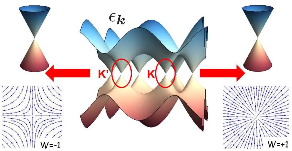
Figure 1: Top: the energy spectrum $\epsilon({\boldsymbol{k}})$ exhibits two inequivalent points K and K’ where the dispersion relation is linear. Bottom: representation of the vector field $(\cos\phi_{\boldsymbol{k}},\sin\phi_{\boldsymbol{k}})$ where $\phi_{\boldsymbol{k}}$ is the relative phase between the two components of the wave function. The winding of the wave function around K and K’ is characterized by a winding number $w=\pm 1$.

Such annihilation of Dirac points is not reachable in graphene because it would imply a large deformation of the lattice impossible to achieve.Pereira ; Goerbig:08 However it may be observed in various different physical systems, including several beyond condensed matter, which share common properties or interesting analogies with graphene. Such systems are now called ”artificial graphenes”. The list of such systems is now very long and has been reviewed in a recent paper.Polini:13 In the present paper, we will not address the huge literature on the subject but only restrict ourselves to several realizations of artificial graphenes in which the motion and merging of Dirac points has been achieved and studied.

The outline of this paper is as follows: we first start with a brief introduction to the electronic properties of graphene. Then we show that the motion and merging of Dirac points follows a universal scenario with a peculiar spectrum at the merging transition: it is quadratic along one direction and linear in the perpendicular direction. This peculiar structure of the spectrum, named semi-Dirac, is accompanied by the annihilation of the windings numbers attached to the Dirac points, signature of the topological character of the transitionVolovik . In the next sections, we consider several experimental works in which this transition has been observed. We emphasize that each experimental situation is not a simple reproduction of graphene physics, but either allows for the investigation of situations not reachable in graphene or opens new directions of research proper to this situation. We conclude by a generalization to various mechanisms of merging of Dirac points.

II Brief reminder about graphene

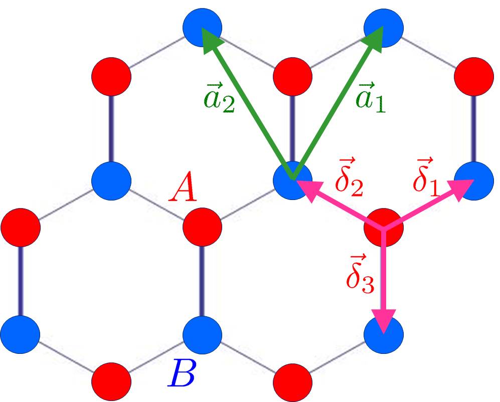
Figure 2: The ”honeycomb” lattice consists in an hexagonal Bravais lattice and two atoms per unit cell. We have represented the elementary vectors ${\boldsymbol{a}}_{1},{\boldsymbol{a}}_{2}$ of the Bravais lattice and the three vectors ${\boldsymbol{\delta}_{1}},{\boldsymbol{\delta}_{2}},{\boldsymbol{\delta}_{3}}$ connecting one site to its nearest neighbours.

The valence and conduction bands of graphene are described by a simple tight-binding Hamiltonian

$${\cal H}=-t\sum_{j,j^{\prime}}|\varphi_{j}^{A}\rangle\langle\varphi_{j^{\prime}}^{B}|+h.c.$$ (1)

where the parameter $t$ characterizes the hopping between nearest neighbouring sites. Additional hoppings between higher nearest neighbours exist but are omitted here since they do not change much the physics and do not affect the geometric structure of the wave functions. Here we choose to write the eigenfunctions in the form

$$\psi_{\boldsymbol{k}}({\boldsymbol{r}})=e^{i{\boldsymbol{k}}\cdot{\boldsymbol{R}}}u_{\boldsymbol{k}}({\boldsymbol{r}})\ ,$$ (2)

where the function $u_{\boldsymbol{k}}({\boldsymbol{r}})$ has the periodicity of the real Bravais lattice and of the reciprocal lattice (see discussion about this second statement in appendix A)

$$u_{\boldsymbol{k}}({\boldsymbol{r}}+{\boldsymbol{R}})=u_{\boldsymbol{k}}({\boldsymbol{r}})\qquad,\qquad u_{{\boldsymbol{k}}+{\boldsymbol{G}}}({\boldsymbol{r}})=u_{\boldsymbol{k}}({\boldsymbol{r}})\ .$$ (3)

${\boldsymbol{R}}$ is a vector of the Bravais lattice and ${\boldsymbol{G}}$ is a vector of the reciprocal lattice. In the tight-binding approximation, the cell-periodic part $u_{\boldsymbol{k}}$ is only defined on $A$ and $B$ sites and it is solution of ${\cal H_{\boldsymbol{k}}}u_{\boldsymbol{k}}=E_{\boldsymbol{k}}u_{\boldsymbol{k}}$ with the effective Hamiltonian

$${\cal H}_{\boldsymbol{k}}=\left(\begin{array}[]{cc}0&f_{\boldsymbol{k}}\\ f^{*}_{\boldsymbol{k}}&0\\ \end{array}\right)$$ (4)

and

$$f_{\boldsymbol{k}}=-t(1+e^{i{\boldsymbol{k}}\cdot{\boldsymbol{a}}_{1}}+e^{i{\boldsymbol{k}}\cdot{\boldsymbol{a}}_{2}})\ ,$$ (5)

where ${\boldsymbol{a}}_{1}$ and ${\boldsymbol{a}}_{2}$ are elementary vectors of the Bravais lattice (fig.2). The solutions are

$$u_{\boldsymbol{k}}={1\over\sqrt{2}}\left(\begin{array}[]{c}1\\ \pm e^{i\phi_{\boldsymbol{k}}}\\ \end{array}\right)$$ (6)

with the relative phase $\phi_{\boldsymbol{k}}=\arg(f^{*}_{\boldsymbol{k}})$. They are associated to the energies $\epsilon_{\boldsymbol{k}}=\pm|f_{\boldsymbol{k}}|$ represented in fig.1. The spectrum exhibits two bands touching linearly in two inequivalent points of the Brillouin zone. In the vicinity of these two ”Dirac points”, the Hamiltonian (4) takes the linear form:

$${\cal H}_{\boldsymbol{k}}=c\left(\begin{array}[]{cc}mc&\hbar(\pm q_{x}-iq_{y})\\ \hbar(\pm q_{x}-iq_{y})&-mc\\ \end{array}\right)$$ (7)

where ${\boldsymbol{q}}={\boldsymbol{k}}-{\boldsymbol{K}}^{(^{\prime})}$, $\hbar c=3ta/2$ and $m=0$. This is the form of the Dirac equation for massless particles ($m=0$) in two dimensions. The energy spectrum is linear

$$\epsilon_{\boldsymbol{q}}=\pm\hbar c|{\boldsymbol{q}}|$$ (8)

The velocity $c$ is $300$ smaller than the speed of light. The relative phase $\phi_{\boldsymbol{k}}$ is plotted in fig.3. The winding number around a contour $C$ in reciprocal space is defined asMarzari

$$w(C)={1\over 2\pi}\oint_{C}\vec{\nabla}\phi_{\boldsymbol{k}}\cdot d{\boldsymbol{k}}\ .$$ (9)

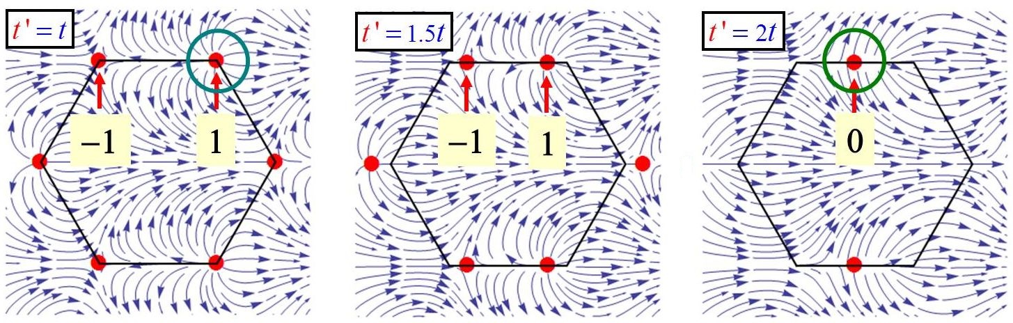
Figure 3: Evolution of the dependence $\phi_{\boldsymbol{k}}$ from the isotropic case $t^{\prime}=t$ to the merging topological transition $t^{\prime}=2t$. At the transition, the opposite winding numbers annihilate. These figures represent the vector field $(\cos\phi_{\boldsymbol{k}},\sin\phi_{k})$.

The two Dirac points are characterized by opposite winding numbers $w=\pm 1$. One important physical signature of this winding structure concerns the Landau levels spectrum $\epsilon_{n}$ obtained from the semi-classical Onsager relationOnsager

$$N(\epsilon_{n})=(n+\gamma){eB\over h}\ ,$$ (10)

where $eB/h$ is the degeneracy of a Landau level and $N(\epsilon)$ is the number of states below energy $\epsilon$, that is the integral of the density of states (These quantities are written by unit area). The phase factor $\gamma=1/2-w(C)/2$ contains the usual Maslov index $1/2$ of the harmonic oscillator and the winding number.Roth ; Fuchs:10 In the vicinity of the Dirac points, the spectrum being linear, the density of states is also linear ($=\epsilon/\hbar^{2}c^{2}$). Application of the Onsager formula leads to a sequence of Landau levels given by grapheneRev

$$\epsilon_{n}(B)=\pm c\sqrt{2n\hbar eB}\qquad,\qquad n\in\mathbb{N}\ .$$ (11)

The observation of this sequence of levels and in particular the existence of a zero energy level were one of the first signatures not only of the strictly 2D character of graphene but also of the spinorial character of the wave functions and the Dirac-like structure of the electronic equation of motion. kim

III Motion and merging of Dirac points

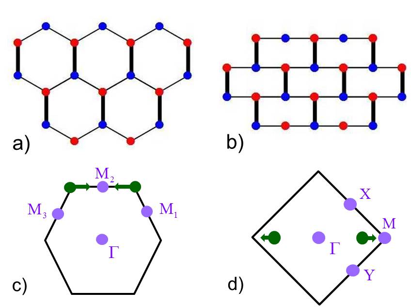
Figure 4: Top: Honeycomb (a) and brickwall (b) lattices. Bottom: position (green dots) of the Dirac points for the isotropic honeycomb and brickwall lattices. Their merging can occur at one of the four TRIMs pictured (purple dots) in the first Brillouin zones for the honeycomb (c) and the brickwall (d) lattices.

III.1 A toy model

It is first instructive to consider a toy model which consists in a slight variation of the graphene model.Montambaux:09 ; Hasegawa1 ; Dietl ; Guinea:08 One of the three hopping parameters introduced in eq.(5) is now fixed to a different value $t^{\prime}>t$ (the vertical bars in fig.4). The function $f_{\boldsymbol{k}}$ defined above is now given by

$$f_{\boldsymbol{k}}=-(t^{\prime}+te^{i{\boldsymbol{k}}\cdot{\boldsymbol{a}}_{1}}+te^{i{\boldsymbol{k}}\cdot{\boldsymbol{a}}_{2}})\ .$$ (12)

The position of the Dirac points being given by $f_{\boldsymbol{k}}=0$, it is easy to check, and this is shown of fig.5, that when the parameter $t^{\prime}$ increases, the Dirac points move until they merge at the M₂ point (as defined in fig.4-c). This happens for the critical value of the merging parameter $\beta\equiv t^{\prime}/t=2$. Above this value, $f_{\boldsymbol{k}}=0$ has no solution, implying the existence of a gap in the energy spectrum. The evolution of the spectrum is shown in fig.5: when $t^{\prime}$ increases, the two Dirac points tend to approach each other, the velocity along the merging line decreases until it vanishes at the transition $t^{\prime}=2t$. At the transition, the spectrum is quite interesting, it is quadratic along the direction of merging, but stays linear along the perpendicular direction. More precisely, it has the form

$$\epsilon({\boldsymbol{q}})=\pm\sqrt{\left({q_{x}^{2}\over 2m_{*}}\right)^{2}+c^{2}q_{y}^{2}}$$ (13)

where $m_{*}=2/(3ta^{2})$ and $c=3ta$ ($\hbar=1$). This hybrid spectrum, massive-massless, has been baptized ”semi-Dirac”. Pickett This critical spectrum corresponds to a topological Lifshitz transition, since the two winding numbers associated to the Dirac points have annihilated and the winding number around the point M is now $0$. At this point and in its vicinity, the thermodynamic and transport properties are quite new.Montambaux:09 ; Dietl ; Adroguer The density of states associated to this hybrid spectrum scales as $\sqrt{\epsilon}$ and since the winding number is zero, the Onsager-Roth formula leads to a dependence of the Landau levels of the form $\epsilon_{L}(B)\propto[(n+1/2)B]^{2/3}$.Dietl

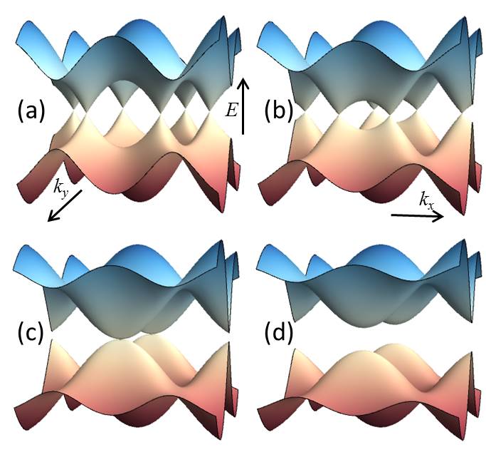
Figure 5: Evolution of the energy spectrum for the toy model (4,12), with $\beta=t^{\prime}/t=1(a),1.5(b),2(c),2.5(d)$. At the critical value $\beta=2$, the spectrum is semi-Dirac.

III.2 A universal Hamiltonian

A natural question now arises whether this toy model is generic of more general situations. We have shown that this scenario of merging is actually quite general.Montambaux:09 The demonstration is as follows. Consider a general situation where objects (these can be atoms, molecules, classical wave scatterers, semiconducting micropillars, etc.) on a lattice are described by a Hamiltonian whose general structure is given in eq.(4). The function $f$ describes the coupling between $A$ and $B$ sites. Quite generally, the function $f_{\boldsymbol{k}}$ can be written in the form (this function has the periodicity of the Bravais lattice, see Appendix A):

$$f_{\boldsymbol{k}}=\sum_{m,n}t_{mn}e^{i{\boldsymbol{k}}\cdot{\boldsymbol{R}}_{mn}}\ ,$$ (14)

where ${\boldsymbol{R}}_{mn}$ are vectors of a Bravais lattice. For example in the previous toy model, we have simply $t_{00}=t^{\prime}$, $t_{01}=t_{10}=t$ and other parameters $t_{mn}=0$. In general, depending on the values of these parameters, there may be either no Dirac point, one or several pairs $({\boldsymbol{D}},-{\boldsymbol{D}})$ of Dirac points. The merging of two partners necessarily occurs when ${\boldsymbol{D}}=-{\boldsymbol{D}}\ (\text{mod}\,{\boldsymbol{G}}^{pq})$ where ${\boldsymbol{G}}^{pq}=p{\boldsymbol{a}}^{*}_{1}+q{\boldsymbol{a}}^{*}_{2}$ is a reciprocal lattice vector. Therefore merging occurs at points ${\boldsymbol{D}}^{pq}={\boldsymbol{G}}^{pq}/2$. There are four inequivalent (they cannot be deduced from each other by a translation of a reciprocal lattice vector) such points called Time Reversal Invariant Momenta (TRIM) corresponding to $(p,q)=(0,0),(0,1),(1,0)$ or $(1,1)$. The merging of a pair of Dirac points occurs at such a point ${\boldsymbol{D}}^{pq}$ when the parameter $f_{{\boldsymbol{D}}^{pq}}=\sum_{m,n}t_{mn}e^{i{\boldsymbol{D}}^{pq}\cdot{\boldsymbol{R}}_{mn}}$ vanishes. Since the product ${\boldsymbol{G}}^{pq}\cdot{\boldsymbol{R}}_{mn}=2\pi(pm+qn)$, this parameter $f_{{\boldsymbol{D}}^{pq}}=\sum_{m,n}t_{mn}\beta^{pq}_{mn}$, where we have defined $\beta^{pq}_{mn}=(-1)^{pm+qn}$. In the previous example for graphene, merging at the M₂ point ($p=1,q=1$) occurs when the parameter $f_{{\boldsymbol{D}}^{pq}}=t_{00}-t_{01}-t_{10}=t^{\prime}-2t$ vanishes.

Let us now consider the vicinity of this merging point by an expansion of the wave vector. Writing ${\boldsymbol{k}}={\boldsymbol{D}}^{pq}+{\boldsymbol{q}}$, we find

$$f_{{\boldsymbol{D}}^{pq}+{\boldsymbol{q}}} = f_{{\boldsymbol{D}}^{pq}}+i{\boldsymbol{q}}\cdot\sum_{mn}\beta^{pq}_{mn}t_{mn}{\boldsymbol{R}}_{mn}$$ (15)

$$- {1\over 2}\sum_{mn}\beta^{pq}_{mn}t_{mn}({\boldsymbol{q}}\cdot{\boldsymbol{R}}_{mn})^{2}+\cdots\ .$$

The linear term is purely imaginary. It defines a direction $\hat{y}$ and a velocity

$$c^{pq}=\sum_{m,n}\beta^{pq}_{mn}t_{mn}R_{y,mn}\ .$$ (16)

Once this local axis is defined, consider the quadratic terms. They are of the form $q_{x}^{2},q_{x}q_{y},q_{y}^{2}$ where $\hat{x}$ is defined has the direction perpendicular to $\hat{y}$. At lowest order, we keep only the term $q_{x}^{2}$. Then the function $f_{{\boldsymbol{D}}^{pq}+{\boldsymbol{q}}}$ has the expansion

$$f_{{\boldsymbol{D}}^{pq}+{\boldsymbol{q}}}=f_{{\boldsymbol{D}}^{pq}}+ic^{pq}q_{y}+{q_{x}^{2}\over 2m^{pq}}\ .$$ (17)

Of course, the parameters $c^{pq}$, $m^{pq}$ and $\Delta^{pq}$ depend on the position $(p,q)$ of the merging point, and they will be now simply denoted by $c$, $m_{*}$ and $\Delta_{*}$. The effective mass $m_{*}$ and the merging parameter $\Delta_{*}$ are given by

$${1\over m_{*}} = -\sum_{mn}\beta^{pq}_{mn}t_{mn}R^{2}_{x,mn}\ ,$$ (18)

$$\Delta_{*} = \sum_{mn}\beta^{pq}_{mn}t_{mn}\ .$$ (19)

We conclude that, in the vicinity of the merging point at a TRIM, the Hamiltonian as the universal form:

$${\cal H}({\boldsymbol{q}})=\left(\begin{array}[]{cc}0&\Delta_{*}+{q_{x}^{2}\over 2m_{*}}+icq_{y}\\ \Delta_{*}+{q_{x}^{2}\over 2m_{*}}-icq_{y}&0\\ \end{array}\right)$$ (20)

where the parameters depend on the position of the merging point. In addition to being independent of the details of the microscopic parameters, we stress that this is the minimal Hamiltonian which describes the coupling between two Dirac points of opposites charges and their merging.Montambaux:09 The dispersion relation given by

$$\epsilon({\boldsymbol{q}})=\pm\sqrt{\left(\Delta_{*}+{q_{x}^{2}\over 2m_{*}}\right)^{2}+c^{2}q_{y}^{2}}\ .$$ (21)

is shown in fig.6.

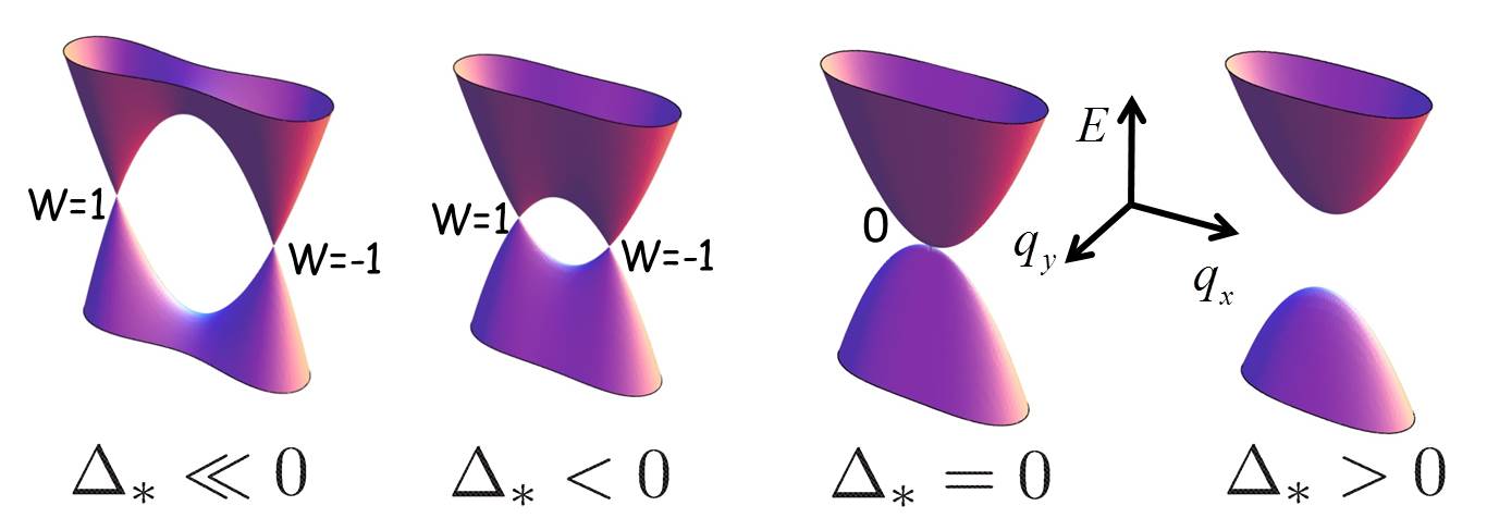
Figure 6: Universal scenario for the merging transition between the Dirac phase ($\Delta_{*}<0$) and the gapped phase ($\Delta_{*}>0$).

When $\Delta_{*}<0$, it describes a pair of massless Dirac points with opposite winding numbers.Montambaux:09 The two Dirac points at positions $\pm\sqrt{-2m^{*}\Delta_{*}}$ are separated by a saddle point (Van Hove singularity) at energy $|\Delta_{*}|$. At the critical value $\Delta_{*}=0$, the spectrum has the hybrid ”semi-Dirac” form, quadratic in the $\hat{x}$ direction and linear in the $\hat{y}$ direction. The density of states associated to this hybrid spectrum scales as $\sqrt{\epsilon}$. When $\Delta_{*}>0$, a gap opens. The Hamiltonian (20) describes a continuous cross-over between the limit of uncoupled valleys corresponding to the situation in graphene and the merging of the Dirac points. It allows for a continuous description of the coupling between valleys which increases as the energy of the saddle decreases.

In refs.Dietl, ; Montambaux:09, ; Adroguer, , we have studied the thermodynamic and transport properties of this Hamiltonian, in particular the spectrum in a magnetic field. The evolution of the Landau levels from the Dirac phase $\Delta_{*}<0$ to the gapped phase $\Delta_{*}>0$ is shown in fig.7. In the Dirac phase, the Landau levels vary as $\sqrt{nB}$ (eq.11) with a double valley degeneracy. When the energy of the Landau levels reaches the energy of the saddle point $|\Delta_{*}|$, the two-fold valley degeneracy is lifted. At the critical value $\Delta_{*}=0$, the energy levels scale as $[n+1/2)B]^{2/3}$, a consequence of the $\sqrt{\epsilon}$ dependence of the density of states and of the cancellation of the winding number. Above the transition, in the gapped phase, one recovers usual Landau levels varying linearly with the field.

Figure 7: Evolution of the Landau spectrum as a function of the parameter $\Delta^{*}/B^{2/3}$. The sequence of Hall numbers is indicated in the gaps. The blue line corresponds to the energy of the saddle point separating Dirac cones. For more details, see ref.Montambaux:09, .

In ref.Montambaux:09, it was proposed a slightly more general toy model than the one presented above. It consists of a lattice with four different hopping parameters $t_{00},t_{01},t_{10},t_{11}$. In this case, the merging parameter $\Delta_{*}$ depends on the merging point (one of the four TRIMs) and it is given by eq.(19), that is:

$$\Delta_{*}=t_{00}+(-1)^{p}t_{01}+(-1)^{q}t_{10}+(-1)^{p+q}t_{11}$$ (22)

Put it differently, the merging or emergence of Dirac points is possible at the TRIM $(p,q)$ where this parameter vanishes. Fig.8 shows the motion of the Dirac points between the four different TRIMs under appropriate variation of hopping parameters. We shall see in the next section that this tight-binding model has been achieved experimentally. The particular choice of parameters $t_{00}=t^{\prime}$, $t_{01}=t_{10}=t$, $t_{11}=0$ corresponds to the ”brickwall” lattice, very similar to graphene, but with a rectangular symmetry, see Figs. 4 and 9.

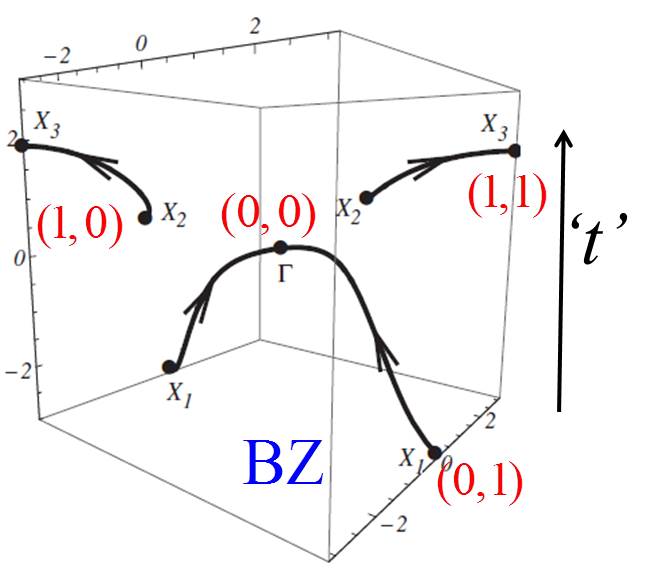
Figure 8: Motion of Dirac points when varying the parameters of eq.(22). Here ${}^{\prime}t^{\prime}$ represents a variation of hopping parameters which is not detailed here. See ref.Montambaux:09, for the choice of parameters.

The scenario described by the universal Hamiltonian was proposed in 2009. It was immediately realized that the merging of Dirac points could not be reached in graphene, because it would need an applied strain along one direction of about $23\%$.Pereira ; Goerbig:08 This scenario remained considered as a theoretical exercise for a few years. It was predicted to be accessible in the organic conductor $\alpha$-(BEDT-TTF)₂I₃ under high pressure but has not been observed yet.Kobayashi It took a few years to highlight this scenario in various systems emulating the physics of electronic propagation in graphene. These systems are now called ”artificial graphenes”. Their interest lies in the strong experimental challenge for their realization and the variety of physical questions they raise. In the next sections, we detail several experiments on artificial graphenes in which the motion and merging of Dirac points have been highlighted.

IV Cold atoms

electrons $\displaystyle\longrightarrow$ atoms atomic lattice $\displaystyle\longrightarrow$ optical lattice

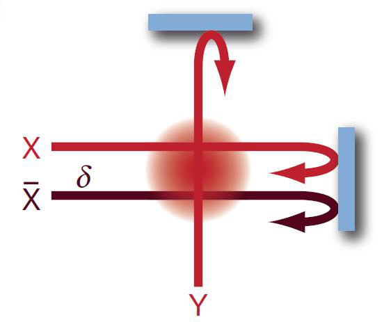
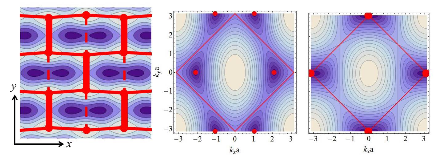
Figure 9: Top: Three lasers beams create a two-dimensional potential (see ref.Tarruell:12, for details). Bottom left: Spatial dependence of this optical potential described by a tight-binding model. The atomic sites corresponds to the minima of the potential (light blue) Tunneling is avoided along the maxima of the potential (dark blue). The lines represent the hopping amplitudes ($t$ : horizontal lines, $t^{\prime}$ thick vertical lines. $t^{\prime\prime}$ dashed vertical lines). Bottom right: isoenergy lines and position of the Dirac points for $t^{\prime}=t$ and $t^{\prime}=2t$ ($t^{\prime\prime}=0$).

In condensed matter the structure of the atomic orbitals makes it impossible to realize a brickwall lattice. However, such a lattice can be achieved with ultracold atoms trapped in an optical lattice.Tarruell:12 An appropriate potential profile, schematized in fig.9, is generated with three stationary laser beams. With appropriate laser intensities (denoted $V_{X}$ and $V_{\overline{X}}$, see fig.9 and ref.Tarruell:12, ), the energy spectrum of the trapped atoms exhibits two bands with a pair of Dirac points, well described by the brickwall tight-binding model with essentially two parameters $t$ and $t^{\prime}$, which can be tuned by modification of the laser parameters. A third parameter $t^{\prime\prime}$ may be introduced for a better quantitative modeling. The motion and merging of these points are properly tuned by variation of the laser parameters. In order to probe the spectrum and its evolution, a low-energy cloud of fermionic atoms ⁴⁰K occupies the bottom of the lower band and is submitted to a constant force $F$ inducing a linear time dependence $\hbar k=Ft$ of the quasi-momentum ${\boldsymbol{k}}$, so that the energy $\epsilon({\boldsymbol{k}})$ oscillates with time. This phenomenon is called a Bloch oscillation.Bloch ; Dahan If the motion is slow (small $F$), a state $k(t)$ moves adiabatically along the energy band $\epsilon(k(t))$. If the motion is fast (large $F$) and when two bands become close to each other, an atom initially in the lower band has a finite probability to tunnel to the upper band. Near a Dirac point, the tunneling probability is given by the Landau-Zener-Stückelberg theory and is related to the gap $E_{g}$ between the two bands:Zener

$$P_{Z}=e^{\displaystyle-\pi{(E_{g}/2)^{2}\over cF}}\ .$$ (23)

$F$ is the force which drives the linear time dependence of the wave vector $k$ and $c$ is the velocity (fig. 10). By measuring the proportion of atoms transferred to the upper band after a single Bloch oscillation, it is possible to reconstruct the energy spectrum in the vicinity of the Dirac points, therefore to highlight the motion and merging of Dirac points under distortion of the lattice induced by appropriate variations of the laser parameters. Two geometries are of interest, when the force is applied along or perpendicularly to the merging line (fig.11-a,d).

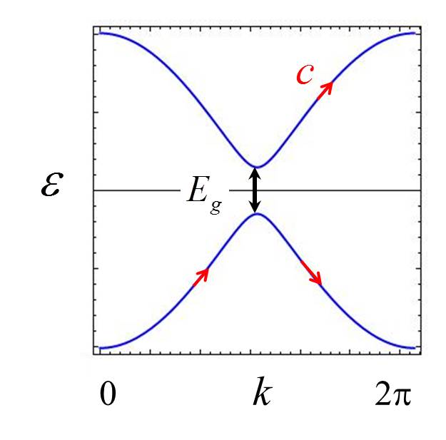
Figure 10: A atom initially in the lower band submitted to a constant force $F$ may tunnel from the lower to the upper band.

IV.1 Single Zener tunneling

In this first situation, the force $F$ in applied along the $\hat{y}$-direction perpendicular to the merging line so that the fermionic cloud hits the two Dirac points in parallel (fig.11-a). An atom in a state with finite $q_{x}$ performs a Bloch oscillation along a direction of constant $q_{x}$ and may tunnel into the upper band with the probability

$$P_{Z}^{y}=\displaystyle e^{\displaystyle-\pi{(\Delta_{*}+{q_{x}^{2}\over 2m^{*}})^{2}\over c_{y}F}}\ .$$ (24)

In the gapped (G) phase ($\Delta_{*}>0$), the tunneling probability is vanishingly small. Deep in the Dirac (D) phase ($\Delta_{*}<0$), when the distance between the two Dirac points $2q_{D}=2\sqrt{2m_{*}|\Delta_{*}|}$ is larger than the size of the cloud, the tunnel probability is also small (fig.11-b). It is maximal close to the merging transition. In order to simulate the finite width of the fermionic cloud, the probability (24) has to be averaged over a finite range of $q_{x}$. Then the three parameters of the universal Hamiltonian can be related to the tight-binding parameters and then, via a simple ab initio calculation, to the two parameters $(V_{X},V_{\overline{X}})$ of the optical potential to finally obtain the probability as a function of these two parameters. As shown in fig.11, we have found that the laser amplitude $V_{\overline{X}}$ mainly tunes the merging parameter $\Delta_{*}$ while the laser amplitude $V_{X}$ essentially tunes the velocity $c_{y}$. One obtains without adjustable parameter an excellent agreement with the experimental result (compare Figs. 11-b-c).Lim:12 In particular we find that the probability is maximal for $\Delta\simeq-\langle q_{x}^{2}\rangle/2m_{*}$ that is inside the Dirac phase as found experimentally.

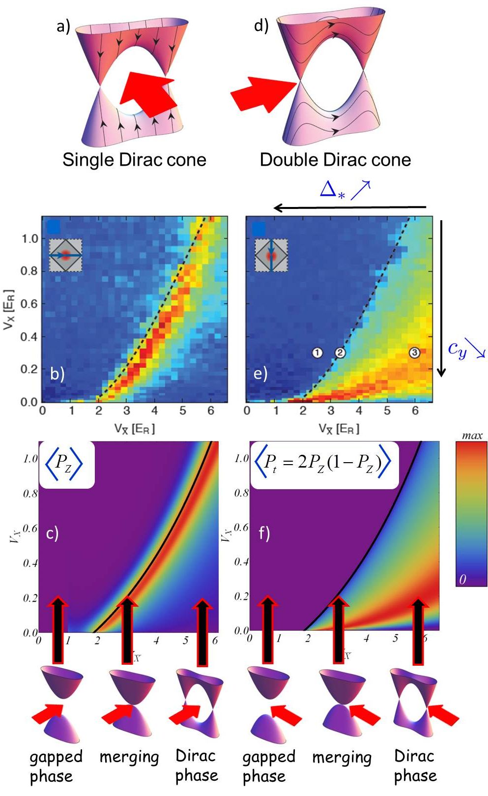
Figure 11: A low energy fermionic cloud of cold atoms is accelerated towards a pair of Dirac points (a,b). The probability to tunnel to the upper band depends on the vicinity of the Dirac cones. This probability is represented as a function of the two laser parameters $V_{X}$ and $V_{\overline{X}}$, see refs.Tarruell:12, ; Lim:12, . Top figures b,e : experimental results.Tarruell:12 The dashed line indicates the merging transition (2) separating the gapped phase (1) and the Dirac phase (3). Figures c,f : theory.Lim:12 After a single Zener tunneling event, the probability is maximal close to the merging line (left figures). When a double Zener tunneling, the probability in maximal inside the Dirac phase.

IV.2 Double Zener tunneling

The force $F$ is now applied along the merging direction $\hat{x}$ so that the fermionic cloud hits the two Dirac points in series (fig.11-d). Along one Bloch oscillation, an atom of fixed $q_{y}$ performs now two Zener transitions in a row, each of them being characterized by the tunnel probability

$$P_{Z}^{x}=\displaystyle e^{\displaystyle-\pi{c_{y}^{2}q_{y}^{2}\over c_{x}F}}=\displaystyle e^{\displaystyle-\pi{c_{y}^{2}q_{y}^{2}\over F\sqrt{2|\Delta_{*}|^{2}/m_{*}}}}\ .$$ (25)

Assuming that the two tunneling events are incoherent, the total interband transition probability is

$$P_{t}^{x}=2P_{Z}^{x}(1-P_{Z}^{x})\ .$$ (26)

In the gapped phase, the tunneling probability is again vanishingly small. In the Dirac phase, the interband transition probability [Eq. (26)] is a non-monotonic function of the Zener probability $P_{Z}^{x}$, and it is maximal when $P_{Z}^{x}=1/2$. This explains why the maximum of the tunnel probability is located well inside the D phase (red region in Figs. 11-e,f). Again, after averaging over $q_{y}$, the size of the initial cloud, and relating the parameters $\Delta_{*},m_{*}$ and $c_{y}$ to the microscopic parameters $(V_{X},V_{\overline{X}})$, one finds an excellent agreement with the experimental result (compare Figs. 11-e-f).

IV.3 Interferometry in reciprocal space

The double Zener configuration is particularly interesting because of possible interference between the two Zener events. Assuming the phase coherence is preserved, instead of the probability given by Eq. (26), one expects a resulting probability of the form

$$P_{t}^{x}=4P_{Z}^{x}(1-P_{Z}^{x})\cos^{2}(\varphi/2+\varphi_{d})\ ,$$ (27)

where $\varphi_{d}$ is a phase delay, named Stokes phase, attached to the each tunneling event, and $\varphi=\varphi_{dyn}+\varphi_{g}$ is a phase which has two contributions, a dynamical phase $\varphi_{dyn}$ acquired between the two tunneling events and basically related to the energy difference between the two energy paths, and a geometric phase $\varphi_{g}$. Whereas the dynamical phase carries information about the spectrum, the geometric phase carries information about the structure of the wave functions.Shevchenko ; Lim:13 If the interference pattern could not been observed in the experiment of ref.Tarruell:12, , probably because the optical lattice was actually three-dimensional, it is an experimental challenge to access it directly and to probe the different contributions to the dephasing. More recent experiments with a honeycomb lattice of ultracold atoms have permitted to completely reconstruct the full structure of the wave functions,Schneider ; Tarnowski as expected theoretically. Lim:15

V Microwaves

electrons $\displaystyle\longrightarrow$ microwaves atomic lattice $\displaystyle\longrightarrow$ lattice of dielectric resonators

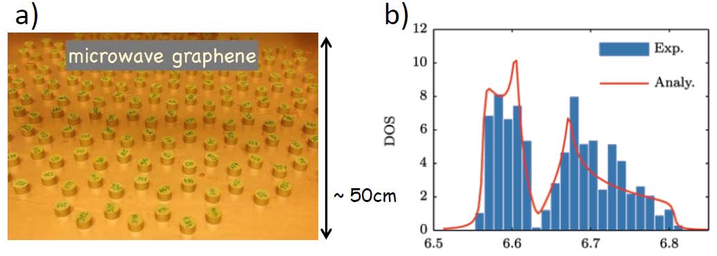
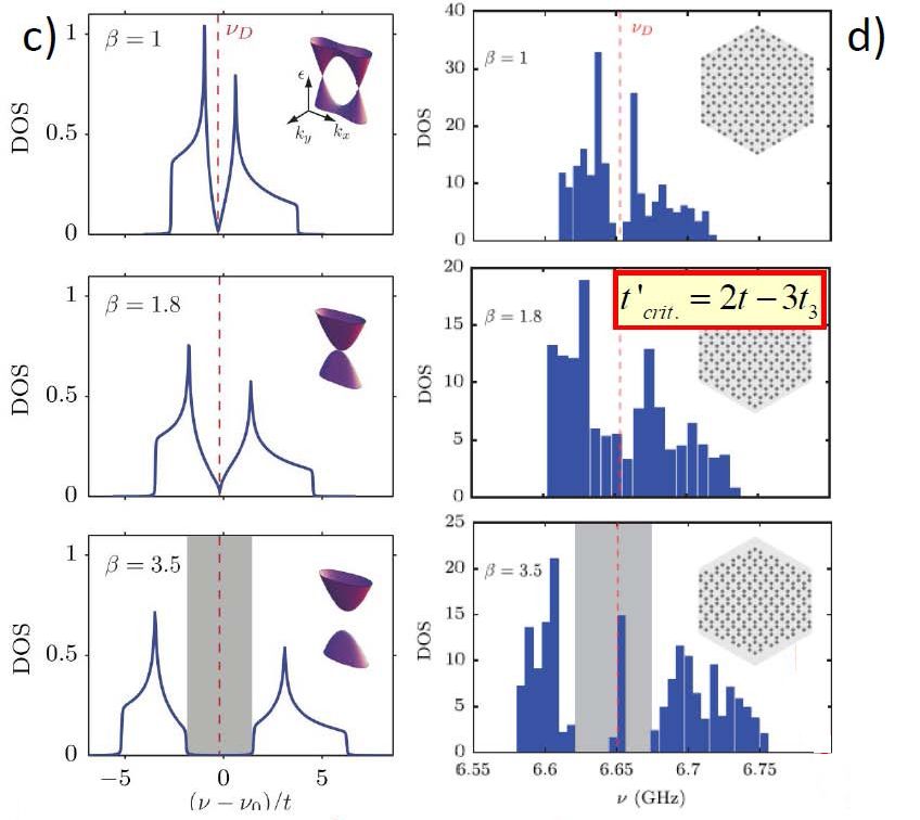
Figure 12: a) Honeycomb lattice of 288 dielectric cylinders. b) Measured density of states well fitted by a tight-binding model with second and third nearest neighbor couplings. c) Expected evolution of the density of states when increasing the anisotropy parameter $\beta=t^{\prime}/t$. d) Experimental evolution of the density of states. The merging transition occurs when $\beta=2-3t_{3}/t$. Under strain, new edge states appear at the band center.

Another artificial graphene has been simulated with a macroscopic setup where cm-size cylindrical dielectric dots replace carbon atoms and microwaves replace the electrons.Bellec:13a A few hundred dots are sandwiched between two metallic plates and are arranged in a 2D honeycomb lattice. A microwave is send through this artificial crystal and is collected by an antenna. The measured signal is related to the local density of states at the place of the antenna. The global density of states is obtained from averaging on the position of the antenna. Therefore this new setup realizes a microwave analog simulator of the quantum propagation of electrons in graphene. The distance between the dots fixes the intensity of the electromagnetic coupling. The frequency of the microwave (a few GHz) is such that its propagation is resonant in the dots and is evanescent outside. Its propagation in the lattice is thus well-described by the same tight-binding model as for graphene. Like in graphene, the second and third neighbour couplings are not negligible (here $t_{2}/t\sim-0.09$, $t_{3}\simeq 0.07$). They do not alter the properties of the Dirac cones, but they change the overall shape of the density of states (fig.12).Bellec:13b

This setup allows for the observation of effects hardly visible or difficult to explore in graphene like the topological transition. Here it can be reached by fabricating an appropriately uniaxial strained lattice. By doing so, the hopping parameters are modified, essentially the nearest neighbour hopping $t^{\prime}$ along the strain direction. The merging parameter $\Delta_{*}$ is given by eq.(19) with the additional parameters $t_{11}=t_{1,-1}=t_{-1,1}=t_{3}$, that is ($p=q=1$, $m=n=1$):

$$\Delta_{*}=t^{\prime}-2t+3t_{3}\ ,$$ (28)

so that the merging transition is expected for the parameter $t^{\prime}=2t-3t_{3}\simeq 1.8t$, as observed experimentally (fig.12).

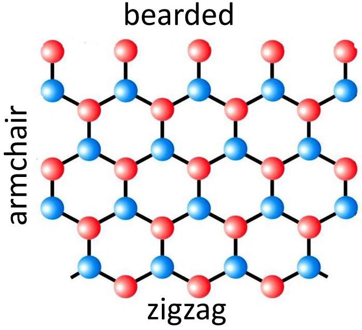
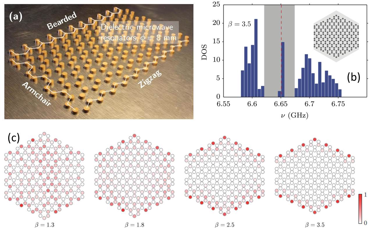
Figure 13: a) The three types of edges, armchair, zigzag and bearded, are achieved on this sample. b) In this lattice under strain, zero energy localized states appear along the armchair edges. c) Evolution of the detected intensity along the armchair edges, showing the appearance of edge states.Bellec:13a

Moreover, the simplicity of this setup allows to probe easily the existence of new exotic states at the edges of the system. The configuration of the edges, well-known to play an important role in graphene but difficult to control, is quite easy to modify here. Fig.13 shows a lattice of dielectric dots with the three types of edges, armchair, zigzag and bearded. The last type of edge, hard to achieve in condensed matter, is quite easy to build here. In this experiment, it has been possible to control the existence of localized states along these different edges, and to control the different types of edge states under applied strain.Bellec:14 Moreover it is possible to measure, for each state, the spatial repartition of the microwave field along the edges. For example, the experiment of fig.12 was performed on a sample with armchair edges which are known not to support localized edge states. However under strain along an appropriate direction, it was predicted that zero energy localized states would appear along the armchair edges.Delplace:11 This evolution is seen on Figs.12-d and 13-c.

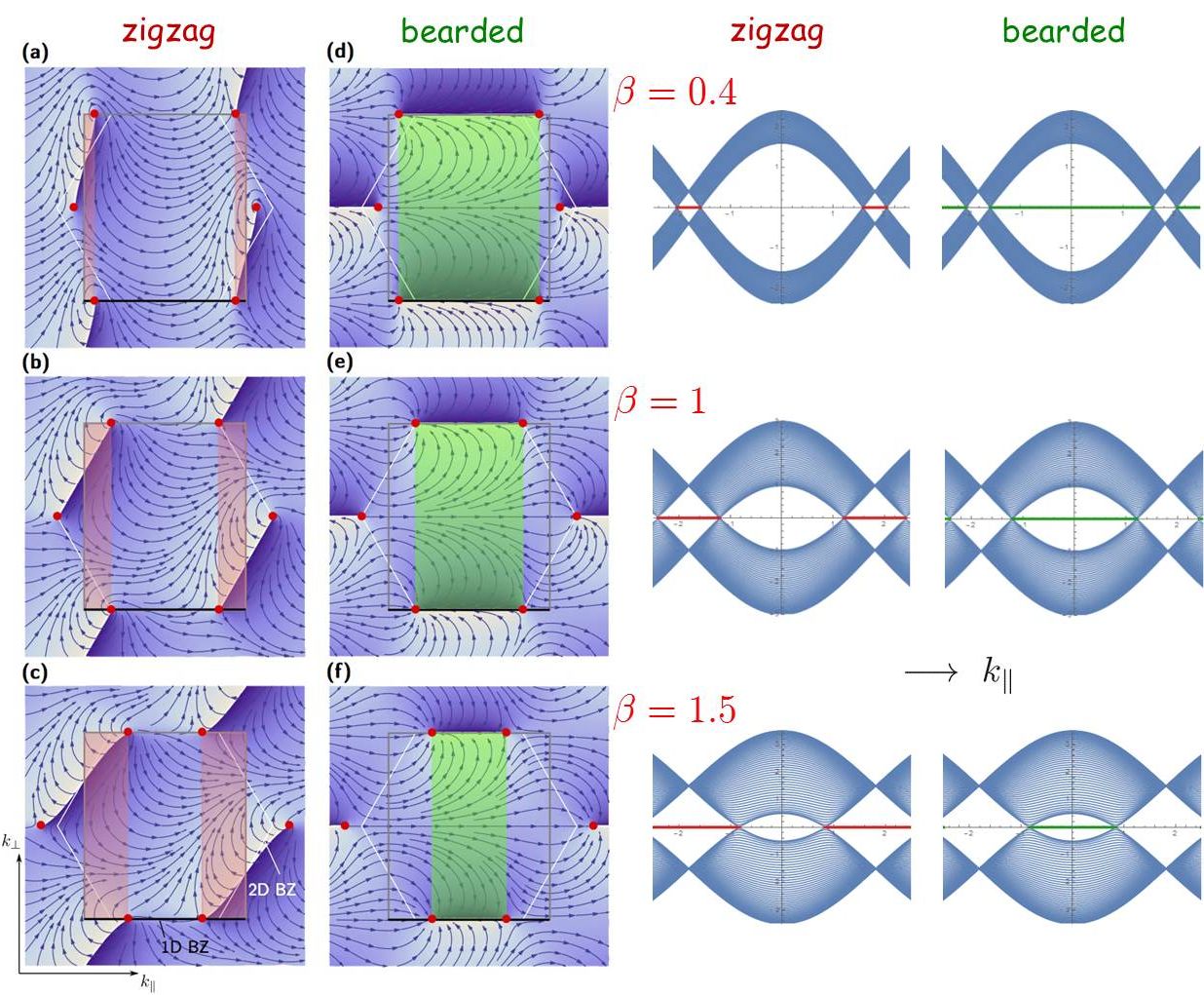
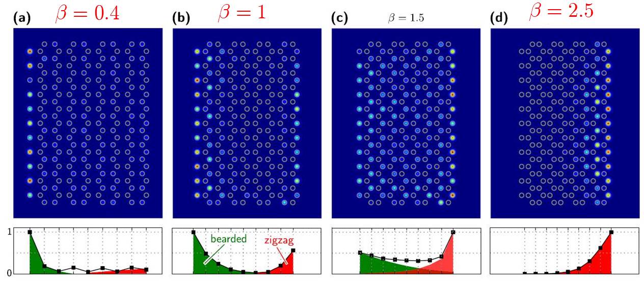
Figure 14: Top left: winding of the phase $\phi_{\boldsymbol{k}}$ in the Brillouin zone. $w(k_{\parallel})$, here $0$ or $1$, measures the number of edges states. There range of existence is colored in pink (zigzag edge states) and green (bearded edge states). Top right : energy spectrum as a function of $k_{\parallel}$, the wave vector along the direction of the edge. Zero energy edge states are represented by red and green lines. When $\beta$ increases, new zigzag states appear at the expense of bearded edge states. This is clearly visible on the experiment (ref. Bellec:14, ) which directly measures the intensity of the microwave at the position of each dot.

It has been shown that the existence of zero energy edge states can be related to a geometric property of the bulk wave functions encoded in a topological quantity bearing similarity with a Zak phase, a one-dimensional equivalent of the Berry phase.Delplace:11 First the Hamiltonian, that is the function $f_{\boldsymbol{k}}$, has to be written consistently with the type of edge, as explained in ref.Delplace:11, . Then the topological quantity

$$w(k_{\parallel})={1\over 2\pi}\int{\partial\phi_{\boldsymbol{k}}\over\partial k_{\perp}}dk_{\perp}$$ (29)

measures the winding of the wave function along the direction $\perp$ perpendicular to the edges. It directly gives the number of edge states with wave vector $k_{\parallel}$ along a given edge. Fig.14 shows the winding of the phase and values of $k_{\parallel}$ for which zero energy edge states exists. It is seen that zigzag and bearded states are complementary and that a strain perpendicular to the edges modify the relative proportion of bearded and zigzag states. When $\beta<1$, new bearded edge states appear at the expense of zigzag edge states. On the opposite, when $\beta>1$, new zigzag edge states appear at the expense of bearded edge states, see bottom fig.14. A similar experiment has been realized in another ”photonic” graphene realized with an array of waveguides arranged in the honeycomb geometry.Segev:13

VI Polaritons

electrons $\displaystyle\longrightarrow$ polaritons atomic lattice $\displaystyle\longrightarrow$ SC micropillars

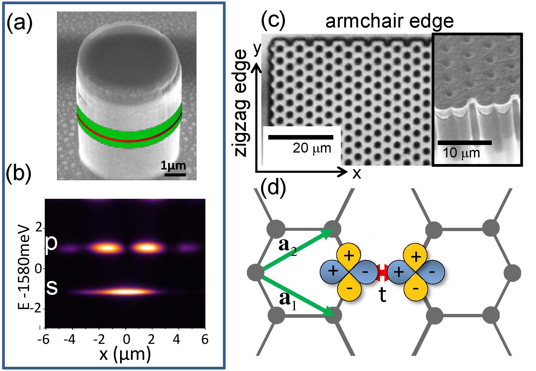
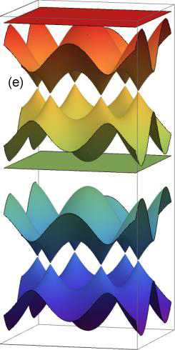
Figure 15: (a) Polaritons in a micropillar: Light is confined in a GaAs cavity (green) where it interacts with quantum well excitons (red). (b) Photonic states are discrete, like the electronic levels in an atom. (c) Honeycomb lattice of overlapping pillars. Polaritons can propagate in this lattice, like electrons do in graphene. (d) Orbital graphene is obtained by coupling the $p_{x}$ and $p_{y}$ states of adjacent sites in the lattice. (e) Band structure exhibiting the $p$-spectrum on top of the $s$-spectrum. The $p$-spectrum resembles the $s$-spectrum, with two additional flat bands (green and red).

Another very interesting setup is a honeycomb lattice of semiconducting (SC) micropillars in which polaritons propagate.c2n0 These mixed light-matter quasiparticles arise from the strong coupling between electronic excitations (so-called excitons) and photons confined in a semiconductor cavity grown by molecular beam epitaxy (fig.15-a). One such cavity, shaped in the form of a micropillar with lateral dimensions of the order of a few microns, behaves like an artificial atom: its discret energy states (orbitals) are the allowed modes of confined photons (fig.15-b). By exciting the cavity with a laser beam, generated electron-hole pairs relax to form polaritons that populate the lowest energy levels. The measurement of energy and angle of the emitted photons allow to reconstruct the polariton spectrum.

By coupling these cavities to make a honeycomb lattice (fig.15-c), one obtains an artificial structure analogue to graphene: the micropillars play the role of carbon atoms, and polaritons which propagate between the pillars play the role of electrons in graphene. The measurement of the dispersion relation of the polaritons by photoluminescence is quite analogous to ARPES experiments in condensed matter. One of the advantages of this system is the possibility to probe the higher orbitals of the pillars, that is the higher energy bands of graphene (fig.15-d). These are inaccessible in graphene due to hybridization with higher bands. Here, the lowest two bands of $s$ symmetry are similar to the $p_{z}$ bands of graphene. The higher energy orbitals, of $p_{x}$ and $p_{y}$ symmetry, form four bands with a remarkable structure consisting of two dispersive bands, which intersect linearly as in graphene, sandwiched between two additional bands that are flat (Figs.15-e and 19). The $s$ and $p$ dispersion relations have been measured by photoluminiscence and are displayed in fig.16.

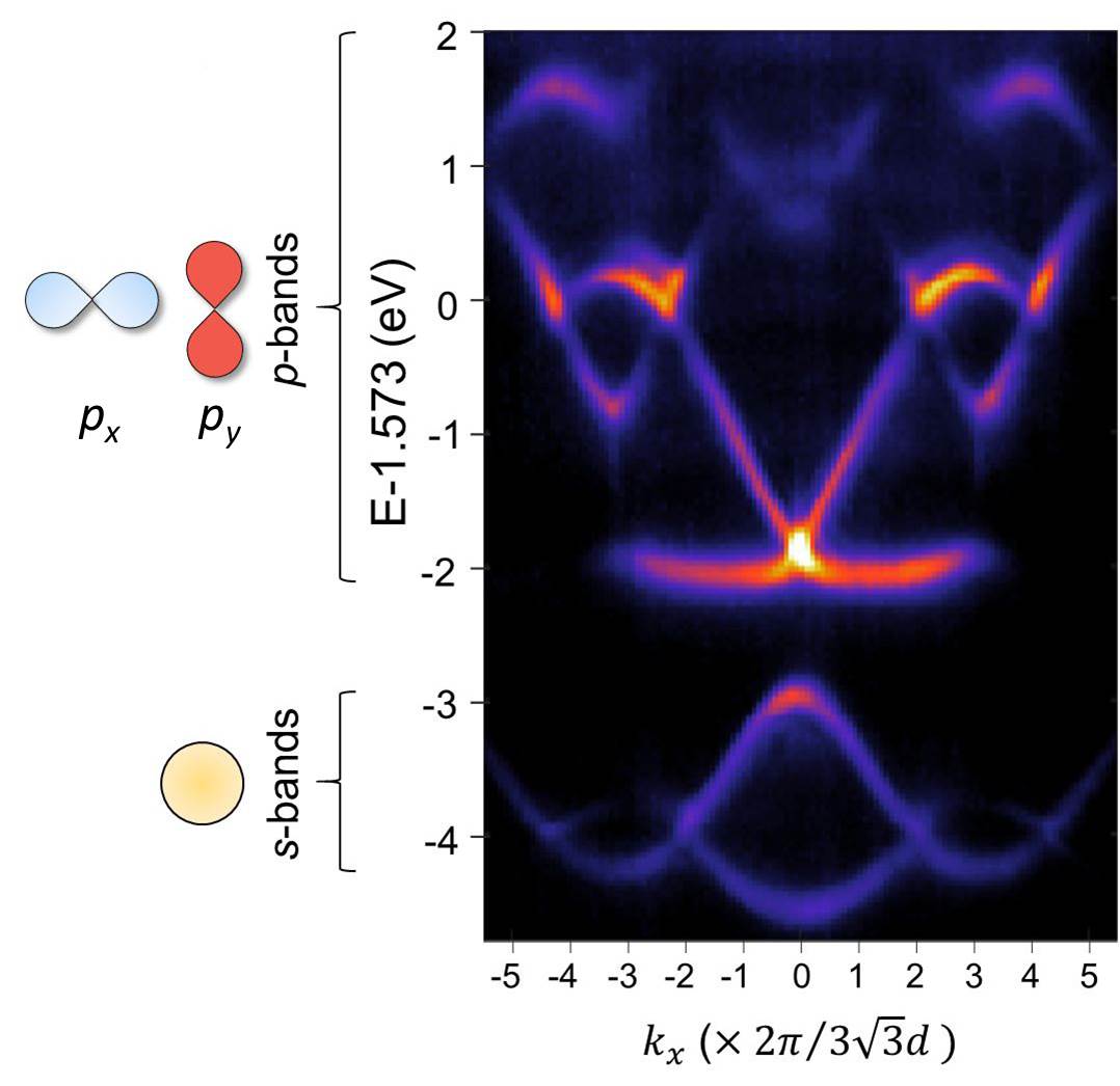
Figure 16: This photoluminescence spectrum shows the two lowest bands of $s$ symmetry and the higher $p$-bands. The lowest flat band is visible while the upper flat band is hardly visible because it is hybridized with higher orbitals.

The $p$-spectrum is well described by a tight-binding model.Wu In the basis of four atomic orbitals ($A$$\infty$, $A$  $\infty$ , $B$$\infty$, $B$  $\infty$ ), the $4\times 4$ Hamiltonian has the form (fig.17)

$${\cal H}_{\boldsymbol{k}}=-t\left(\begin{array}[]{cc}0&Q\\ Q^{\dagger}&0\\ \end{array}\right)\qquad\text{with}\qquad Q=\left(\begin{array}[]{cc}f_{1}&g\\ g&f_{2}\\ \end{array}\right)$$ (30)

with $f_{1}={3\over 4}(e^{i{\boldsymbol{k}}\cdot{\boldsymbol{a}}_{1}}+e^{i{\boldsymbol{k}}\cdot{\boldsymbol{a}}_{2}})$, $f_{2}=\beta+{1\over 4}(e^{i{\boldsymbol{k}}\cdot{\boldsymbol{a}}_{1}}+e^{i{\boldsymbol{k}}\cdot{\boldsymbol{a}}_{2}})$ and $g={\sqrt{3}\over 4}(e^{i{\boldsymbol{k}}\cdot{\boldsymbol{a}}_{1}}-e^{i{\boldsymbol{k}}\cdot{\boldsymbol{a}}_{2}})$. The numerical factors account for the overlap of the orbitals when they are not facing each other, see fig.17. Under anisotropic strain, the anisotropy of hopping parameters is characterized by the parameter $\beta=t^{\prime}/t$ which enters the expression of $f_{2}$.

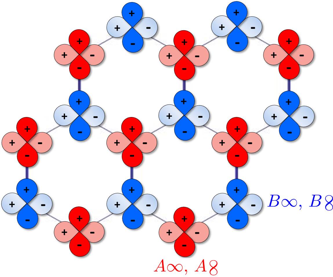
Figure 17: $p_{x}$ and $p_{y}$ orbitals of $A$ and $B$ sites.

This experimental setup is quite rich. The fabrication techniquec2n0 allows to construct honeycomb lattices with arbitrary strain, well described by an anisotropic tight-binding model. By varying the strain, it has been possible to reach the merging of Dirac points in the $s$ band, and to measure directly for the first time the semi-Dirac dispersion relation, as shown in fig.18.

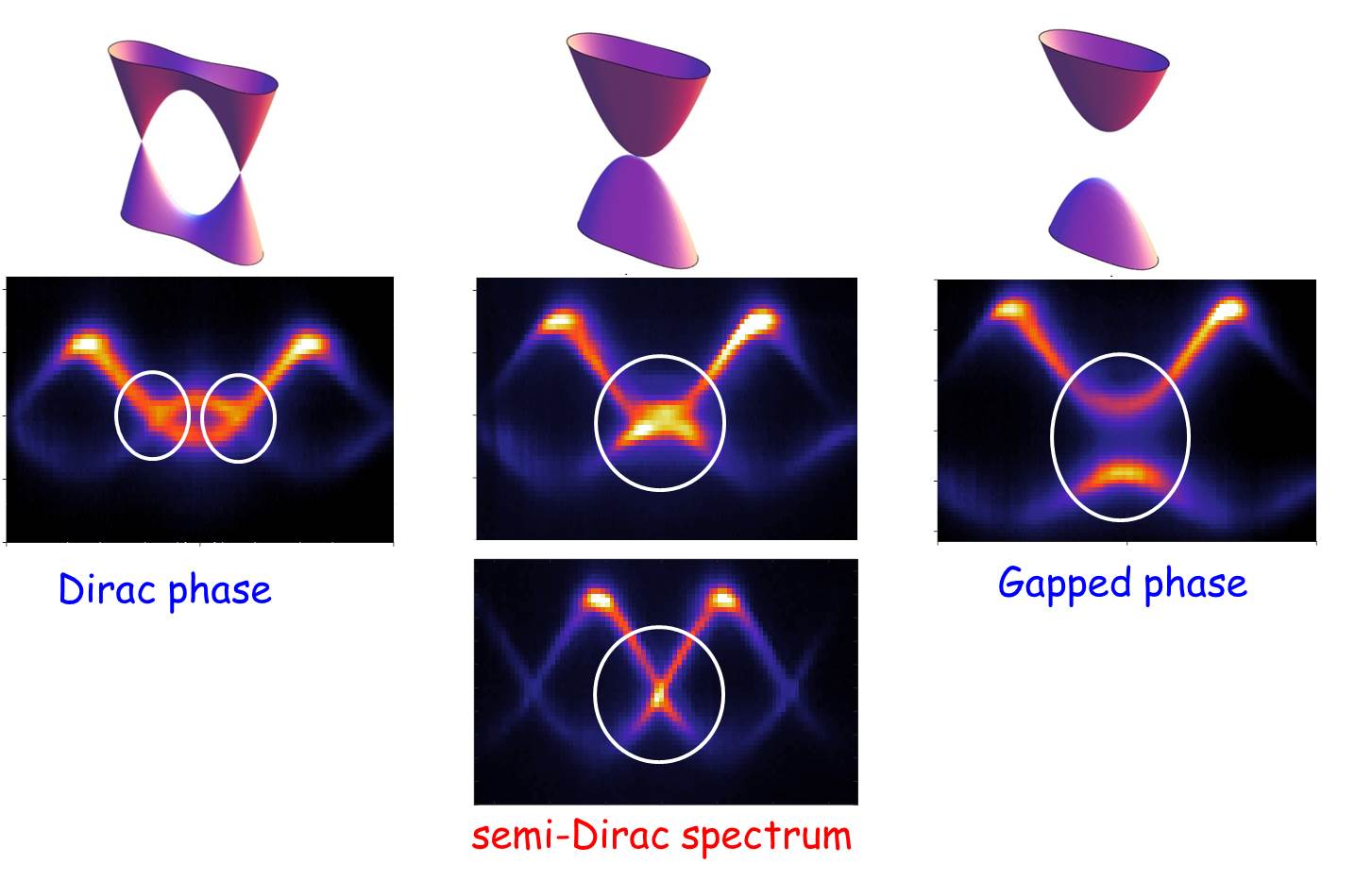
Figure 18: First direct experimental observation of the merging of Dirac points.c2n3 At the transition, when $\beta=2$, the spectrum in the $s$ band is semi-Dirac: it is linear in one direction and it is quadratic in the other direction.

The physics of the $p$-spectrum exhibits many new features. Recent experiments have probed the physics of edge states and the evolution of the $p$-spectrum under strain.

Figure 19: Comparison of the $s$ and $p$ spectra. The right panels show the dispersion relation a long the $k_{\perp}$ direction parallel to the edges. One sees that the ”zero energy” (middle of the spectrum) states appear at complementary edges (zigzag-bearded) and that new edges states of ”finite energy” between the dispersive and the flat bands appear. They have been analyzed in ref.c2n1, .

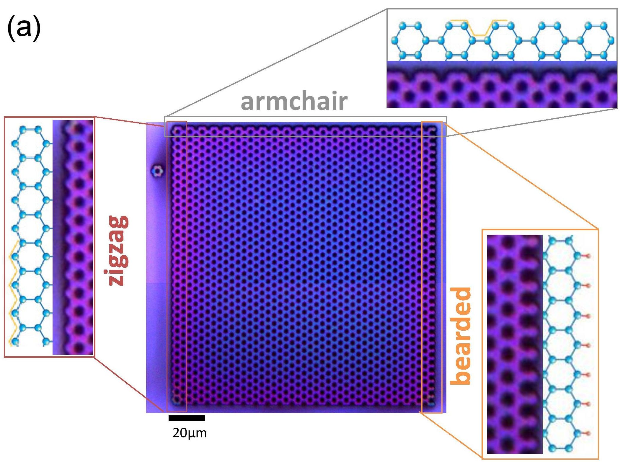
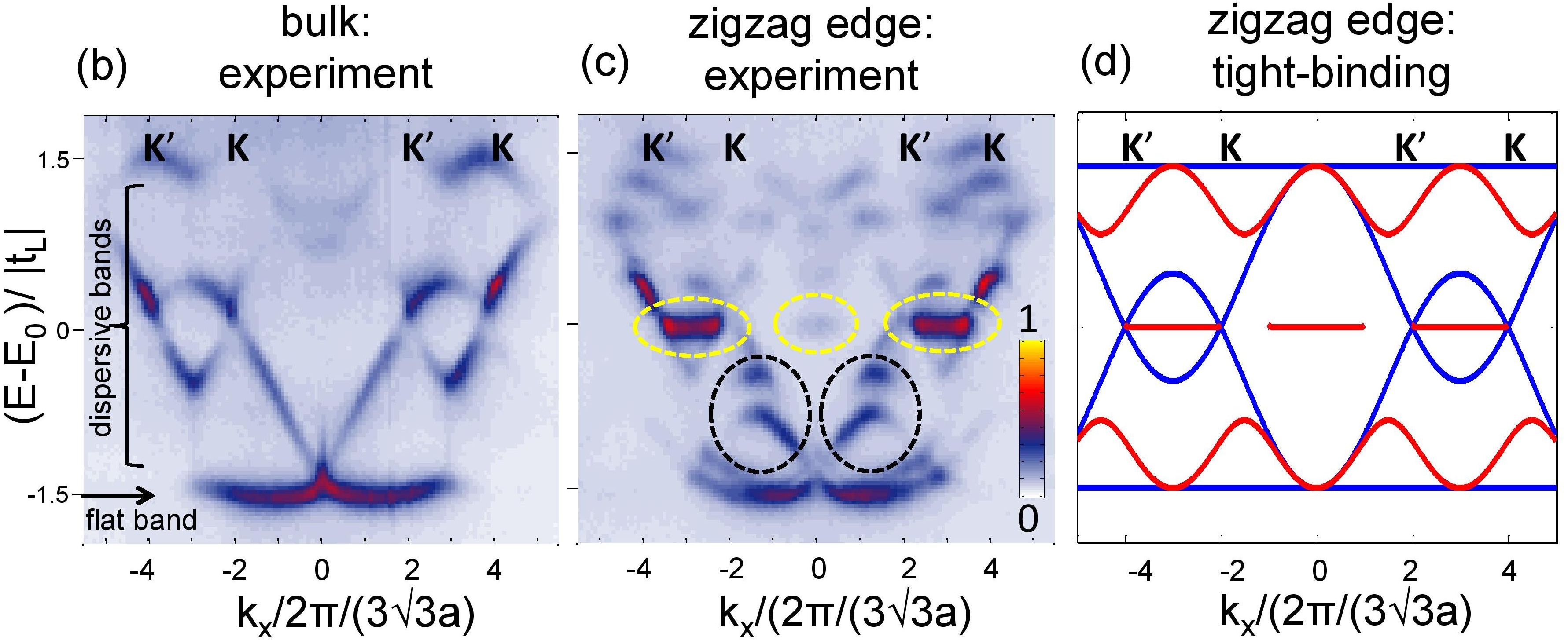
Figure 20: Top: honeycomb lattice of semiconducting micropillars with three types of edges, zigzag, bearded and armchair. Bottom: photoluminescence spectrum in the bulk and close to a zigzag edge. The tight-binding spectrum exhibits the zero energy edge states and new dispersive states (red) between the bulk dispersive states and the flat bands (blue).

Concerning edge states, it was discovered that flat ”zero energy” (in the middle of the $p$-spectrum) edge states exist at positions in momentum space which are complementary to the ones of the $s$ edge states, see figs.19,20. Additionally, new edge states with dispersive character were found for all types of terminations including armchair. Their theoretically analysis is presented in ref.c2n1, .

The most recent experiments concern the evolution of the $p$-spectrum under uniaxial strain. Its evolution in the tight-binding model, compared with the one in the $s$-spectrum, is shown in fig.21. Several remarkable features have to be discussed. The motion of the Dirac points in the middle of the $p$-spectrum follows an evolution opposite to the one of the $s$-spectrum: merging is reached by decreasing the strain parameter $\beta=t^{\prime}/t$ down to the value $\beta=0.5$. The flat bands are deformed as soon as $\beta\neq 1$. A remarkable new feature occurs at the quadratic touching point between the dispersive band and the flat band, either at the top or at the bottom of the spectrum. This quadratic touching point characterized by a winding number $w=2$ splits into a new pair of Dirac points.c2n2 The scenario of emergence of these points is different from the one described in the above sections where the two Dirac points have opposite winding numbers and the merging corresponds to the addition rule of the winding numbers $(+,-)\leftrightarrow 0$. In contrast the two Dirac points here have the same winding number, and the merging/emergence scenario corresponds to addition rule $(+,+)\leftrightarrow 2$.Chong ; Sun ; Dora ; Gail2011 This situation is quite similar to the scenario of splitting of the quadratic touching point observed in bilayer graphene under strain or twist.McCann ; Gail2011 Moreover these new cones are tilted and for the first time a pair of critically tilted cones (that is is with a vanishing velocity in one direction) has been observed.c2n2

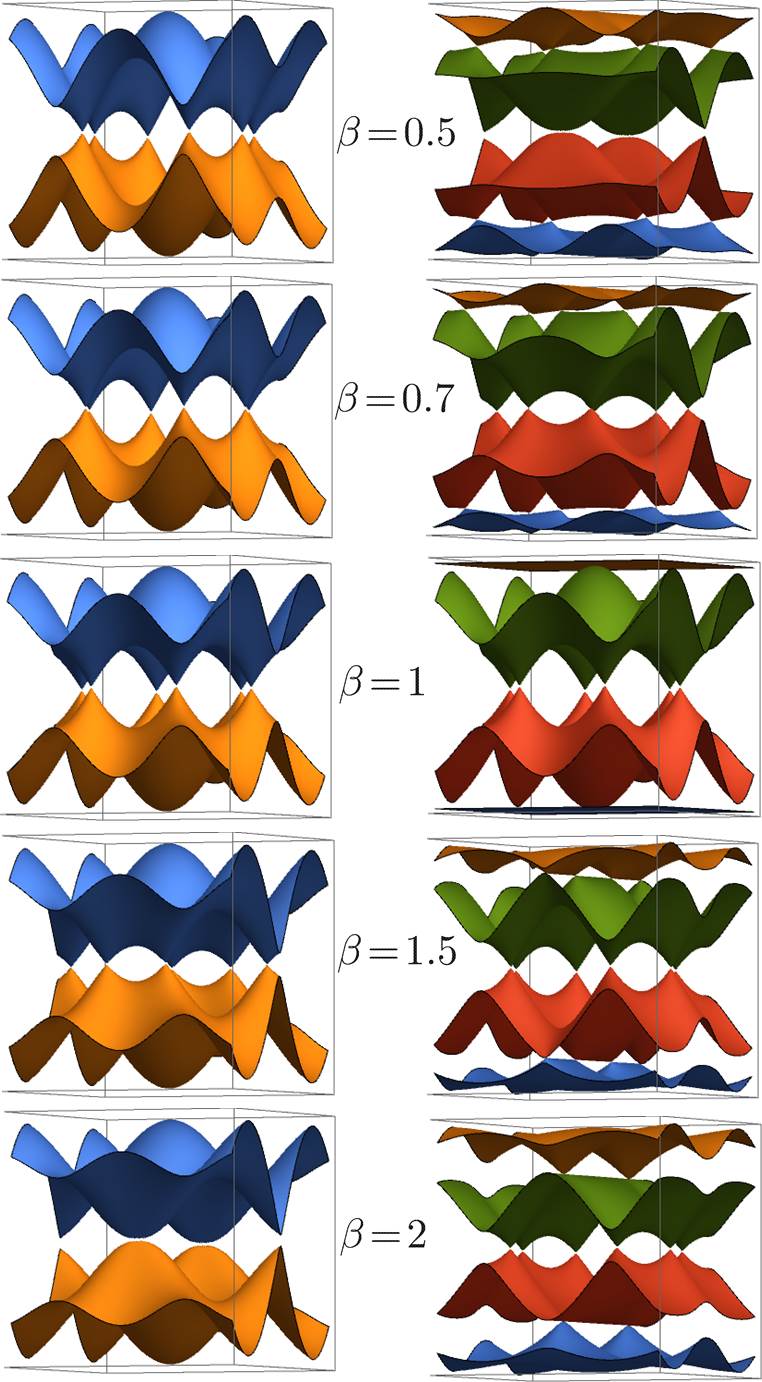
Figure 21: Compared evolutions of the $s$ and $p$ spectra under applied strain. When $\beta\neq 1$, two Dirac points emerge from the flat band at the $\Gamma$ point.

To finish this section, we wish to mention a remarkable duality between the $p$-spectrum and the $s$-spectrum. The energy bands – flat and dispersive – of the $p$-spectrum, $\epsilon^{p}_{flat}$ and $\epsilon^{p}_{disp}$ respectively, are related to those of the $s$-spectrum by the remarkable relation derived in appendix B (consider here only the positive energies, in units of the hopping parameters of the $s$ and $p$ bands):

$$\epsilon_{flat}^{p}(\beta)\,\epsilon_{disp}^{p}(\beta)={3\over 4}\beta\epsilon_{s}\left({1\over\beta}\right)$$ (31)

We have named these $p$-bands, ”flat” and ”dispersive”, but note that the upper (lower) band is flat only when $\beta=1$. From this duality relation, one can draw several conclusions. When $\beta=1$, the extreme $p$ bands are flat, so that the spectrum of the middle bands is the same as the $s$-spectrum (within renormalization by the hopping parameters). Then one understands immediately the complementarity in the spectra and the edge states described above. A variation of the strain parameter $\beta$ ($\beta$ increase or decrease) has opposite effects in the $p$ and $s$ spectra. Moreover bearded states in the $s$ band are complementary to the zigzag states in the $s$ band and vice-versa. The wealth of the effects observed in the orbital $p$ band is a motivation for investigation of more sophisticated features in multiband systems.

VII Phosphorene

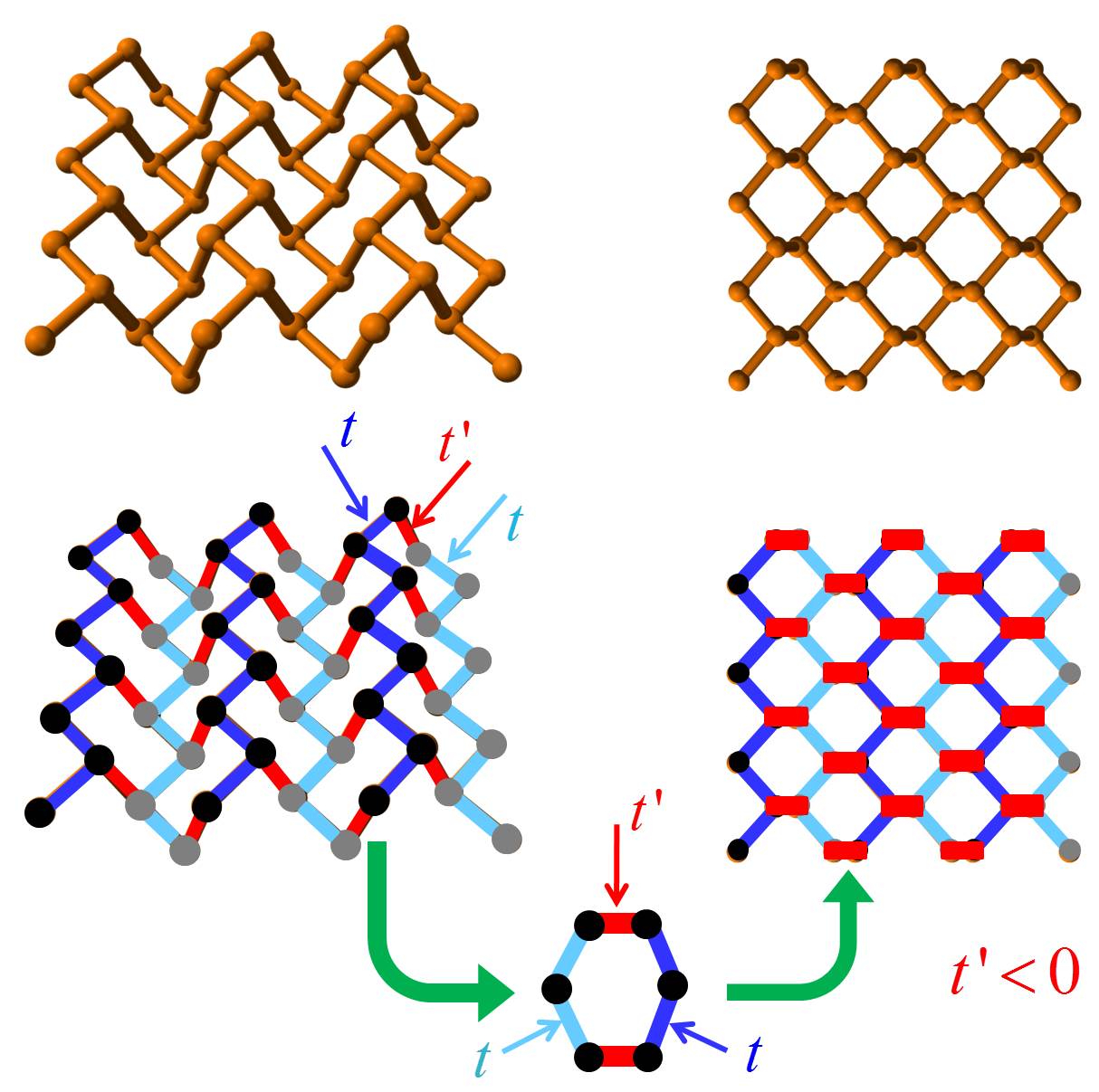
Figure 22: Like graphene, a 2D crystal of phosphorene may be essentially described by a simple tight-binding model with three hopping integrals $t,t,t^{\prime}$. In this case $t^{\prime}$ and $t$ have opposite signs. Left : side view, right : top view.

We finally discuss the properties of a condensed matter two-dimensional system which bears strong similarities with graphene. Phosphorene is a two-dimensional crystal in which carbon atoms are replaced by phosphorus atoms. Because of $sp_{3}$ hybridization of $p$ orbitals (instead of $sp_{2}$ hybridization in graphene), a single sheet of phosphorene is essentially made of two identical planes with horizontal hopping between sites, coupled by an almost vertical hopping (fig.22). At ambient pressure, the electronic spectrum is gapped around the $\Gamma$ point, but under pressure or vertical strain a pair of Dirac points emerges from this point.Kim ; Xiang We show here that this transition follows the scenario of the universal Hamiltonian (20). Although sophisticated large-scale tight-binding simulations have been developed with nine parameters,Rudenko their basic features are captured within our simple toy model with the two parameters of $t,t^{\prime}$, which is used for strained graphene and that is also relevant here.

We have shown above that the merging parameter $\Delta_{*}$ depends on the position of the merging/emergence TRIM point and is given by

$$\Delta_{*}=t^{\prime}+(-1)^{p}t+(-1)^{q}t\ .$$ (32)

In graphene and the realizations discussed above, the two parameters are positive, the transition occurs at the M₂ point so that the relevant combination is $\Delta_{*}=t^{\prime}-2t$. In graphene $t^{\prime}=t$ so that this parameter is negative. Under strain, $t^{\prime}$ increases, so that $\Delta_{*}$ becomes positive and this happens at the topological transition.

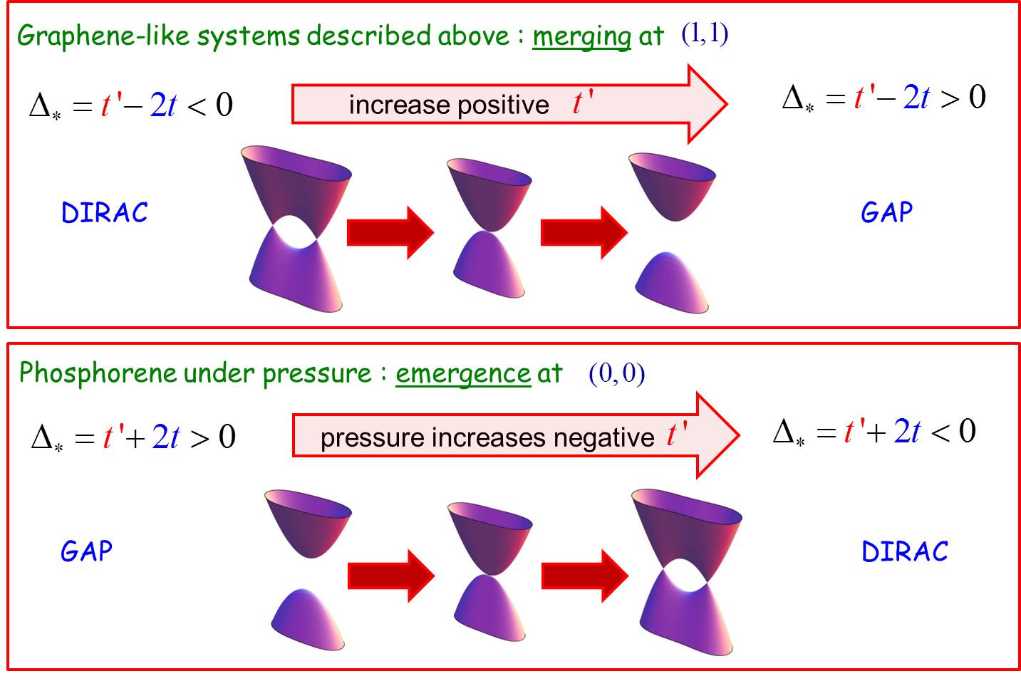
Figure 23: Similarly to graphene, a 2D crystal of phospherene may be essentially described by a simple tight-binding model with three hopping integrals $t,t,t^{\prime}$. In this case $t^{\prime}$ and $t$ have opposite signs.

In phosphorene at ambient pressure, the hopping parameters $t$ and $t^{\prime}$ have opposite signs: $t>0$ and $t^{\prime}<0$. The spectrum is gapped which means that $\Delta_{*}>0$. Under pressure or vertical strain, the Dirac points emerge at the $\Gamma$ point ($p=q=0$) and this phenomenon is therefore driven by the parameter $\Delta_{*}=t^{\prime}+2t$ which becomes negative. The reason is that the amplitude of negative $t^{\prime}$ increases under pressure. This emergence of Dirac points is very well described by the universal Hamiltonian. The calculated evolution of the Landau level spectrum in a complete tight-binding description of phosphorene is quite similar to the expected spectrum obtained from the universal Hamiltonian (compare fig.7 and fig.7 of ref.Pereira2, ).

The two scenarios of merging or emergence in graphene-like structure and phosphorene are summarized in fig.23. We conclude that the merging/emergence of Dirac points in strain (artificial graphene) or phosphorene follow the same universal scenario.

VIII Conclusion

We have described several physical systems where the excitation spectrum exhibits a pair of Dirac cones, such as graphene. The flexibility of these different systems allows one to vary hopping parameters so that these Dirac points can be manipulated: they can move, merge or emerge at special points of high symmetry of the reciprocal lattice.

Each Dirac point is characterized by a winding number $w=\pm 1$, and a pair of Dirac points can merge following two alternative scenarios : either they have opposite ”charge” and this corresponds to the scenario discussed in this paper, $(+-)\leftrightarrow 0$, or they have identical charge and this corresponds to a second merging scenario, $(++)\leftrightarrow 2$, described by another effective Hamiltonian, and which is not discussed in this paper. For a discussion on this second scenario, see the references Gail2012, ; Poincare, . The merging between two Dirac cones is thus a topological transition that may be described by two distinct universality classes, according to whether the two cones have opposite or identical topological charges. We have recently found a system in which the two classes may be observed: indeed, photoluminescence experiments on the $p$-spectrum of a strained honeycomb polariton lattice have shown a very rich variety of Dirac points. Both types of merging have been observed.c2n2 In particular we have highlighted the existence of a pair of Dirac points emerging from the touching point between a quadratic band and a flat band, following the scenario $(+,+)\leftrightarrow 2$. It turns out that under further strain, this pair of Dirac points may merge at another TRIM following the scenario $(+,-)\leftrightarrow 0$.c2n2 ; Montambaux:18 This apparent contradiction is solved by the fact that the winding number is actually defined around a unit vector on the Bloch sphere and that this vector rotates during the motion of the Dirac points.Montambaux:18 These new results open the way for future investigations on the production of Dirac points, their geometric properties and their fate under appropriate variations of external parameters, especially in multiband systems.

Appendix A A remark on two representations of a Bloch function

In the tight-binding picture, the eigenstates, solutions of the Hamiltonian (1) are a combination of atomic orbitals satisfying Bloch theorem. They can be written in the alternative formsBena

$$|\psi_{{\boldsymbol{k}}}\rangle={1\over\sqrt{N}}\sum_{j}e^{i{\boldsymbol{k}}\cdot{\boldsymbol{R}}_{j}}\left(c^{A}_{\boldsymbol{k}}|\varphi^{A}_{j}\rangle+c^{B}_{\boldsymbol{k}}|\varphi^{B}_{j}\rangle\right)$$ (33)

or

$$|\psi_{{\boldsymbol{k}}}\rangle={1\over\sqrt{N}}\sum_{j}\left(e^{i{\boldsymbol{k}}\cdot{\boldsymbol{R}}_{j}^{A}}d^{A}_{\boldsymbol{k}}|\varphi_{j}^{A}\rangle+e^{i{\boldsymbol{k}}\cdot{\boldsymbol{R}}_{j}^{R}}d^{B}_{\boldsymbol{k}}|\varphi_{j}^{B}\rangle\right)$$ (34)

where $\varphi^{A}_{j}$ and $\varphi^{B}_{j}$ are atomic orbitals on sites $(j,A)$ and $(j,B)$. This is the same eigenstate, but these two representations are slightly different. In the first expression, the phase factor in attached to the elementary cell and is common to the $A$ and $B$ sites. This is for example the form found in the Ashcroft and Mermin book (eq. 10.26).Ashcroft In the second writing, each phase factor is attached to the position of each atom, $A$ or $B$. This is for example the notation found in the Wallace paper.Wallace By choosing ${\boldsymbol{R}}_{j}={\boldsymbol{R}}_{j}^{A}$, we have obviously $c_{\boldsymbol{k}}^{A}=d_{\boldsymbol{k}}^{A}$ and $c_{\boldsymbol{k}}^{B}=d_{\boldsymbol{k}}^{B}e^{i{\boldsymbol{k}}\cdot({\boldsymbol{R}}^{B}-{\boldsymbol{R}}^{A})}=d_{\boldsymbol{k}}^{B}e^{i{\boldsymbol{k}}\cdot{\boldsymbol{\delta}}_{3}}$, $\delta_{3}$ being the $AB$ distance (fig.2). The two representations of the same eigenfunction are of the form

$$\psi({\boldsymbol{r}}) = e^{i{\boldsymbol{k}}\cdot{\boldsymbol{R}}}\,u_{I,{\boldsymbol{k}}}({\boldsymbol{r}})$$ (35)

$$\psi({\boldsymbol{r}}) = e^{i{\boldsymbol{k}}\cdot{\boldsymbol{r}}}\,u_{II,{\boldsymbol{k}}}({\boldsymbol{r}})$$ (36)

where ${\boldsymbol{r}}$ is the position and ${\boldsymbol{R}}$ is a vector of the Bravais latttice, position of the elementary cell in the lattice. Note that the function $u_{I,{\boldsymbol{k}}}({\boldsymbol{r}})$ has the periodicity of the reciprocal lattice, while $u_{II,{\boldsymbol{k}}}({\boldsymbol{r}})$, which is the most common representation, does not.

In the tight-binding model (1), the wave function is defined only on the $A$ and $B$ sites so that the normalized wave functions can be written in the spinorial form:

$$\text{either}\qquad u_{I,{\boldsymbol{k}}} = \left(\begin{array}[]{c}c^{A}_{\boldsymbol{k}}\\ c^{B}_{\boldsymbol{k}}\\ \end{array}\right)={1\over\sqrt{2}}\left(\begin{array}[]{c}1\\ \pm e^{i\phi_{I,{\boldsymbol{k}}}}\\ \end{array}\right)$$ (41)

$$\text{or}\qquad u_{II,{\boldsymbol{k}}} = \left(\begin{array}[]{c}d^{A}_{\boldsymbol{k}}\\ d^{B}_{\boldsymbol{k}}\\ \end{array}\right)={1\over\sqrt{2}}\left(\begin{array}[]{c}1\\ \pm e^{i\phi_{II,{\boldsymbol{k}}}}\\ \end{array}\right)\ .$$ (46)

They are solutions of the $2\times 2$ Hamiltonian

$${\cal H}_{i,{\boldsymbol{k}}}=\left(\begin{array}[]{cc}0&f_{i,{\boldsymbol{k}}}\\ f^{*}_{i,{\boldsymbol{k}}}&0\\ \end{array}\right)$$ (47)

with

$$\text{either}\qquad f_{I,{\boldsymbol{k}}} = -t(1+e^{i{\boldsymbol{k}}\cdot{\boldsymbol{a}}_{1}}+e^{i{\boldsymbol{k}}\cdot{\boldsymbol{a}}_{2}})$$ (48)

$$\text{or}\qquad f_{II,{\boldsymbol{k}}} = -t(e^{i{\boldsymbol{k}}\cdot{\boldsymbol{\delta}}_{3}}+e^{i{\boldsymbol{k}}\cdot{\boldsymbol{\delta}}_{1}}+e^{i{\boldsymbol{k}}.{\boldsymbol{\delta}}_{2}})$$ (49)

and the relative phase between the two components of the wave function is given by $\phi_{i,{\boldsymbol{k}}}=\arg(f_{i,{\boldsymbol{k}}}^{*})$, so that

$$\phi_{II,{\boldsymbol{k}}}=\phi_{I,{\boldsymbol{k}}}-{\boldsymbol{k}}\!\cdot\!{\boldsymbol{\delta}}_{3}\ .$$ (50)

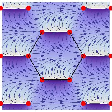
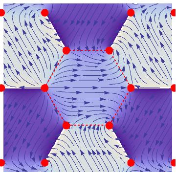
Figure 24: Representation of the phases $\phi_{I,{\boldsymbol{k}}}$ (left) and $\phi_{II,{\boldsymbol{k}}}$ (right), via the vector field $(\cos\phi,\sin\phi)$. The phase $\phi_{I,{\boldsymbol{k}}}$ has the periodicity of the reciprocal lattice. The phase $\phi_{II,{\boldsymbol{k}}}$ has a triple periodicity. This phase has been measured directly in interferometry experiments with a honeycomb lattice of cold atomsSchneider ; Tarnowski ; Lim:15 and in ARPES experiments on graphene (fig.26).Mucha

In the first representation, the phase $\phi_{I,{\boldsymbol{k}}}$ has the periodicity of the reciprocal lattice : $\phi_{I,{\boldsymbol{k}}+{\boldsymbol{G}}}=\phi_{I,{\boldsymbol{k}}}$, see fig.24. Obviously, because of the linear term ${\boldsymbol{k}}\!\cdot\!{\boldsymbol{\delta}}_{3}$ related to the $A-B$ distance, the phase $\phi_{II,{\boldsymbol{k}}}$ does not have this periodicity but a triple periodicity (fig.24).

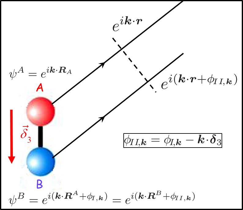
Figure 25: The waves emitted by the sites of the honeycomb lattice can be described by a ”two-source” interference pattern.Mucha

What is the physical interpretation of these two phases $\phi_{I}$ and $\phi_{II}$ ? The periodic honeycomb lattice can be represented by a two-source emitterMucha corresponding to the two sublattices, see fig.25. $\phi_{I,{\boldsymbol{k}}}$ is the relative phase between the two emitters, that is the phase delay between the waves emitted by the two sites. It does not account for the relative position between these two sites. If ${\boldsymbol{k}}\!\cdot\!{\boldsymbol{r}}$ represents the phase emitted by atoms $A$ at any point ${\boldsymbol{r}}$, the combination ${\boldsymbol{k}}\!\cdot\!{\boldsymbol{r}}+\phi_{II,{\boldsymbol{k}}}$ represents the phase emitted by atoms $B$ at the same point (fig.25). The signals emitted by the two sources construct an interference pattern which depends on the relative position between the two sources. At a position ${\boldsymbol{r}}$ outside the sample, the total electronic wave has the form $e^{i{\boldsymbol{k}}\cdot({\boldsymbol{r}}-{\boldsymbol{R}}_{A})}\psi_{A}+e^{i{\boldsymbol{k}}\cdot({\boldsymbol{r}}-{\boldsymbol{R}}_{B})}\psi_{B}=(1+e^{i\phi_{II,{\boldsymbol{k}}}})e^{i{\boldsymbol{k}}\!\cdot\!{\boldsymbol{r}}}$ so that the intensity $I({\boldsymbol{k}})$ is proportional to $\cos^{2}{\phi_{II,{\boldsymbol{k}}}\over 2}$, as measured in ARPES experiments, see fig.26.

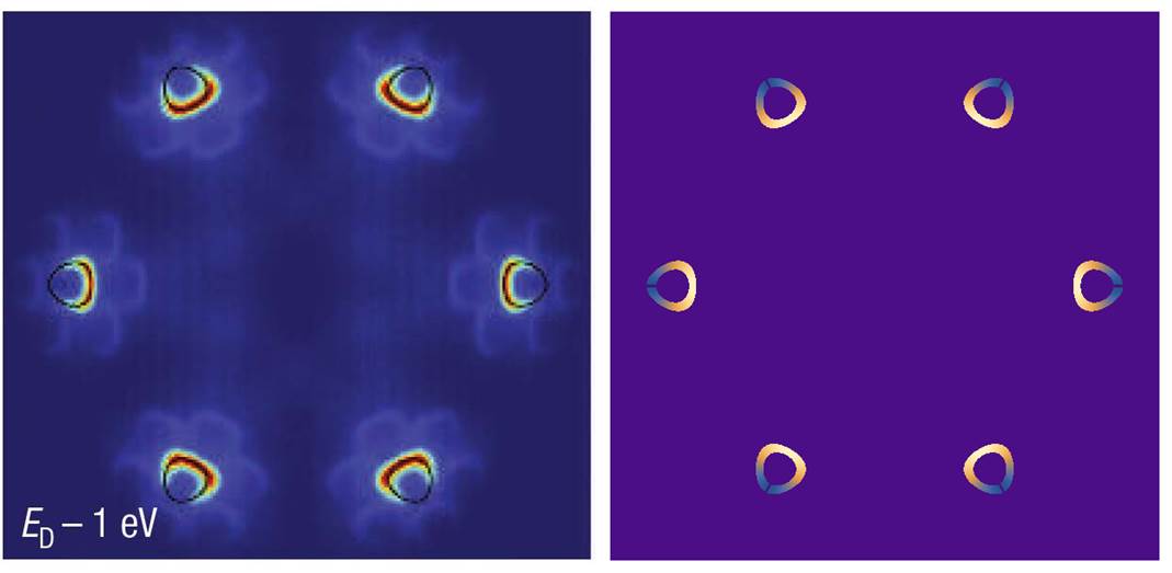
Figure 26: Left : ARPES measured intensityMucha . Right : Intensity given by $\cos^{2}{\phi_{II,{\boldsymbol{k}}}\over 2}$.

In this paper, we have used the representation I for the writing of the Hamiltonian (4) in its general form (14) which has the periodicity of the reciprocal lattice. It is also used for describing geometric properties of the Hamiltonian and the wave functions, the relation between existence of edge states and the Zak phase.Delplace:11 The phase $\phi_{II,{\boldsymbol{k}}}$ is directly measured in interferometry experiments on cold atomsSchneider ; Lim:15 ; Tarnowski or in ARPES experiments,Mucha because the interference pattern depends on the relative position ${\boldsymbol{\delta}}_{3}$ between atoms $A$ and $B$. This phase does not have the periodicity of the reciprocal lattice.

Appendix B Proof of eq.(31)

This equation relates the dispersion relation of the $p$ bands to the dispersion relation of the $s$ band. The $p$-spectrum consists in four bands of energies named $\pm\epsilon_{flat}$ and $\pm\epsilon_{disp}$. Note that the two ”flat” bands are strictly flat only when $\beta=1$.

Consider first the $s$-spectrum. It is given by $\pm\epsilon_{s}(\beta)$ with $\epsilon_{s}(\beta)=|f_{\boldsymbol{k}}|$, where $f_{\boldsymbol{k}}$ is given by eq.(12). Therefore in units of $t$, it can be written as

$$\epsilon_{s}(\beta)=|\beta+z_{1}+z_{2}|\ ,$$ (51)

where $z_{i}=e^{i{\boldsymbol{k}}\cdot{\boldsymbol{a}}_{i}}$.

Consider now the eigenvalues of the $p$-Hamiltonian (30). Simple algebra shows that the eigenvalues are solutions of the equation

$$\epsilon^{4}-S\epsilon^{2}+P=0\ ,$$ (52)

with

$$\quad S=\text{tr}(QQ^{\dagger})\quad,\quad P=\text{det}(QQ^{\dagger})=|\text{det}\,Q|^{2}\ ,$$ (53)

so that

$$\epsilon_{flat}^{p}\,\epsilon_{disp}^{p}=|\text{det}\,Q|\ .$$ (54)

Writing the elements of the matrix $Q$ as $f_{1}={3\over 4}(z_{1}+z_{2})$, $f_{2}=\beta+{1\over 4}(z_{1}+z_{2})$ and $g={\sqrt{3}\over 4}(z_{1}-z_{2})$, we find

$$\epsilon_{flat}^{p}(\beta)\,\epsilon_{disp}^{p}(\beta) = {3\over 4}\beta\,\left|{z_{1}z_{2}\over\beta}+z_{1}+z_{2}\right|$$ (55)

$$= {3\over 4}\beta\,\left|{1\over\beta}+z_{1}+z_{2}\right|$$

since $|z_{i}|=1$. This proves eq.(31).

References

- (1) A.K. Geim and K.S. Novoselov, Nat. Mat. 6, 183 (2007)
- (2) For a review, see A. H. Castro Neto, N. M. R. Peres, K. S. Novoselov, and A. K. Geim, Rev. Mod. Phys. 81, 109 (2009).
- (3) Dirac Matter, Poincaré Seminar, Prog. Math. Phys. 71 (2016).
- (4) also sometimes called triangular.
- (5) G. Montambaux, F. Piéchon, J.-N. Fuchs and M.-O. Goerbig, Phys. Rev. B 80, 153412 (2009); Eur. Phys. J. B 72, 509 (2009).
- (6) V. M. Pereira, A. H. Castro Neto and N. M. R. Peres, Phys. Rev. B 80, 045401 (2009).
- (7) M.-O. Goerbig, J.-N. Fuchs, G. Montambaux and F. Piéchon, Phys. Rev. B 78,045415 (2008)
- (8) M. Polini, F. Guinea, M. Lewenstein, H. C. Manoharan and V. Pellegrini, Nature Nanotech. 8, 625 (2013).
- (9) G. Volovik, The Universe in a Helium Droplet, Oxford uni versity press (2009).
- (10) For a discussion between frequent confusion between the winding number and the Berry phase, see C.-H. Park and N. Marzari, Phys. Rev. B 84, 205440 (2011).
- (11) L. Onsager, Phil. Mag. 43, 1006 (1952); I.M. Lifshitz and A.M. Kosevich, Sov. Phys. J.E.T.P. 2, 636 (1956).
- (12) L. Roth, Phys. Rev. B 145, 434 (1966).
- (13) J.-N. Fuchs, F. Piéchon, G. Montambaux and M.-O. Goerbig, Eur. Phys. J. B 77, 351 (2010).
- (14) Y. Zhang, Y.-W. Tan, H. L. Stormer, and P. Kim, Nature 438, 201 (2005).
- (15) Y. Hasegawa, R. Konno, H. Nakano and M. Kohmoto, Phys. Rev. B 74, 033413 (2006).
- (16) P. Dietl, F. Piéchon and G. Montambaux, Phys. Rev. Lett. 100, 236405 (2008).
- (17) B. Wunsch, F. Guinea and F. Sols, New J. Phys. 10, 103027 (2008).
- (18) V. Pardo and W. E. Pickett, Phys. Rev. Lett. 102, 166803 (2009); S. Banerjee, R. R. P. Singh, V. Pardo and W. E. Pickett, Phys. Rev. Lett. 103, 016402 (2009).
- (19) P. Adroguer, D. Carpentier, G. Montambaux and E. Orignac, Phys. Rev. B 93, 125113 (2016).
- (20) A. Kobayashi, S. Katayama and Y. Suzumura, Science and Tech. of Adv. Mat. 10, 024309 (2009); A. Kobayashi, Y. Suzumura, F. Piéchon and G. Montambaux, Phys. Rev. B 84, 075450 (2011).
- (21) L. Tarruell, D. Greif, T. Uehlinger, G. Jotzu, and T. Esslinger, Nature 483, 302 (2012).
- (22) F. Bloch, Z. Phys. 52, 555 (1929).
- (23) M. Dahan, E. Peik, J. Reichel, Y. and C. Salomon, Phys. Rev. Lett. 76, 4508 (1996).
- (24) L.D. Landau, Phys. Z. Sow. 2, 46 (1932); C. Zener, Proc. R. Soc. London A 137, 696 (1932); see also C. Wittig, J. Phys. Chem. B 109, 8428 (2005).
- (25) L.-K. Lim, J.-N. Fuchs, and G. Montambaux, Phys. Rev. Lett. 108, 175303 (2012); J.-N. Fuchs, L.-K. Lim and G. Montambaux, Phys. Rev. A 86, 063613 (2012).
- (26) S. N. Shevchenko, S. Ashhab, and F. Nori, Phys. Rep. 492, 1 (2010).
- (27) L.-K. Lim, J.-N. Fuchs, and G. Montambaux, Phys. Rev. Lett. 112, 155302 (2014); Phys. Rev. A. 91, 042119 (2015).
- (28) T. Li, L. Duca, M. Reitter, F. Grust, E. Demler, M. Endres, M. Schleier-Smith, I. Bloch and U. Schneider, Science 352, 1094 (2016).
- (29) M. Tarnowski, M. Nuske, N. Fläschner, B. Rem, D. Vogel, L. Freystatzky, K. Sengstock, L. Mathey and C. Weitenberg, Phys. Rev. Lett. 118, 240403 (2017).
- (30) L.-K. Lim, J.-N. Fuchs, and G. Montambaux, Phys. Rev. A 92, 063627 (2015).
- (31) M. Bellec, U. Kuhl, G. Montambaux, and F. Mortessagne, Phys. Rev. Lett. 110, 033902 (2013).
- (32) M. Bellec, U. Kuhl, G. Montambaux and F. Mortessagne, Phys. Rev. B 88, 115437 (2013).
- (33) M. Bellec, U. Kuhl, G. Montambaux and F. Mortessagne, New J. Phys. 16, 113023 (2014).
- (34) P. Delplace, D. Ullmo, and G. Montambaux, Phys. Rev. B 84, 195452 (2011).
- (35) M. C. Rechtsman, Y. Plotnik, J. M. Zeuner, A. Szameit and M. Segev, Phys. Rev. Lett. 111, 103901 (2013).
- (36) T. Jacqmin, I. Carusotto, I. Sagnes, M. Abbarchi, D. Solnyshkov, G. Malpuech, E. Galopin, A. Lemaître, J. Bloch and A. Amo, Phys. Rev. Lett. 112, 116402 (2014).
- (37) C. Wu, D. Bergman, L. Balents, and S. Das Sarma, Phys. Rev. Lett. 99, 070401 (2007).
- (38) M. Milićević et al., in preparation.
- (39) M. Milićević, T. Ozawa, G. Montambaux, I. Carusotto, E. Galopin, A. Lemaître, L. Le Gratiet, I. Sagnes, J. Bloch, and A. Amo, Phys. Rev. Lett. 118, 107403 (2017).
- (40) M. Milićević, G. Montambaux, T. Ozawa, I. Sagnes, , A. Lemaître, L. Le Gratiet, A. Harouri, J. Bloch, and A. Amo, arXiv:1807.08650
- (41) Y.D. Chong, X.-G. Wen and M. Soljac̆ić, Phys. Rev. B 77, 235125 (2008).
- (42) K. Sun, H. Yao, E. Fradkin and S. A. Kivelson, Phys. Rev. Lett. 103, 046811 (2009).
- (43) B. Dora, I.F. Herbut and R. Moessner, Phys. Rev. B 90, 045310 (2014).
- (44) E.McCann and V.I.Fal’ko, Phys.Rev.Lett. 96, 086805 (2006).
- (45) R. de Gail, M.O. Goerbig, F. Guinea, G. Montambaux, and A.H. Castro Neto, Phys. Rev. B 84, 045436 (2011).
- (46) G. Montambaux, L.-K. Lim, J.-N. Fuchs and F. Piéchon, arXiv:1804.00781
- (47) J. Kim, S. S. Baik, S. H. Ryu, Y. Sohn, S. Park, B.-G. Park, J. Denlinger, Y. Yi, H. J. Choi and K. S. Kim, Science 349 723 (2015).
- (48) An applied electric field may also drives this transition. The evolution of the electronic spectrum in a field has been observed directly by ARPES measurements. Z. J. Xiang, G. J. Ye, C. Shang, B. Lei, N. Z. Wang, K. S. Yang, D. Y. Liu, F. B. Meng, X. G. Luo, L. J. Zou, Z. Sun, Y. Zhang and X. H. Chen, Phys. Rev. Lett. 115, 186403 (2015)
- (49) A.N. Rudenko, S. Yuan and M.I. Katsnelson, Phys. Rev. B 92, 085419 (2015).
- (50) J. M. Pereira and M. I. Katsnelson, Phys. Rev. B 92, 075437 (2015).
- (51) R. de Gail, J.-N. Fuchs, M.O. Goerbig F. Piéchon and G. Montambaux, Physica B 407, 1948 (2012); R. de Gail, M.O. Goerbig and G. Montambaux, Phys. Rev. B 86, 045407 (2012).
- (52) For a review, see M.O. Goerbig and G. Montambaux, in Dirac Matter, Poincaré Seminar, Prog. Math. Phys. 71, 25 (2016).
- (53) C. Bena and G. Montambaux, New J. Phys. 11, 095003 (2009).
- (54) N. W. Ashcroft and N. D. Mermin, Solid State Physics (Saunders, Philadelphia, 1976).
- (55) P. R. Wallace, Phys. Rev. 71, 622 (1947).
- (56) M. Mucha-Kruczynski, O. Tsyplyatev, A. Grishin, E. McCann, V. I. Fal’ko, A. Bostwick and E. Rotenberg, Phys. Rev. B 77, 195403 (2008).