Mixed-Timescale Online PHY Caching for Dual-Mode MIMO Cooperative Networks

Abstract

Recently, physical layer (PHY) caching has been proposed to exploit the dynamic side information induced by caches at base stations (BSs) to support Coordinated Multi-Point (CoMP) and achieve huge degrees of freedom (DoF) gains. Due to the limited cache storage capacity, the performance of PHY caching depends heavily on the cache content placement algorithm. In existing algorithms, the cache content placement is adaptive to the long-term popularity distribution in an offline manner. We propose an online PHY caching framework which adapts the cache content placement to microscopic spatial and temporary popularity variations to fully exploit the benefits of PHY caching. Specifically, the joint optimization of online cache content placement and content delivery is formulated as a mixed-timescale drift minimization problem to increase the CoMP opportunity and reduce the cache content placement cost. We propose a low-complexity algorithm to obtain a throughput-optimal solution. Moreover, we provide a closed-form characterization of the maximum sum DoF in the stability region and study the impact of key system parameters on the stability region. Simulations show that the proposed online PHY caching framework achieves large gain over existing solutions.

I Introduction

Many recent works have shown that wireless network performance can be substantially improved by exploiting caching in content-centric wireless networks [1, 2]. The early works [3, 4, 5] focus on exploiting caching to reduce the backhaul loading. However, the performance of wireless networks is fundamentally limited by interference, and these existing works fail to address this issue. In [6, 7], cache-enabled opportunistic CoMP (PHY caching) is proposed to mitigate interference and improve the spectral efficiency of the physical layer (PHY) in wireless networks with limited backhaul. Beside the common benefits of caching in fixed line networks, DoF gains can be achieved by utilizing a fundamental cache-induced PHY topology change. Specifically, when users’ requested content exists in the cache of several BSs, the BS caches induce dynamic side information, which can be used to cooperatively transmit the requested packets to the users, thus achieving huge DoF gains without requiring high-capacity backhaul links. In practice, the cache storage capacity is limited, and hence, the cache content placement algorithm plays a key role in determining the performance of PHY caching schemes. The existing algorithms can be classified into two types.

Offline cache content placement: Offline cache content placement is adaptive to the long-term popularity distribution in an offline manner. Once the cache content placement phase has finished, the cached content cannot be changed during the content delivery phase. In [6, 7], mixed-timescale optimizations of short-term MIMO precoding and long-term cache content placement are studied to support real-time video-on-demand applications. However, these offline caching algorithms cannot capture the microscopic spatial and temporary popularity variations.

Online cache content placement: Online cache content placement is dynamically adaptive to microscopic spatial and temporary popularity variations during the content delivery phase. Compared to its offline counterpart, it has more refined control over the limited cache resources and thus can potentially achieve a better performance. In [8], online cache placement and request scheduling are studied to support elastic and inelastic traffic in wireless networks. In [9], a framework for joint online forwarding and caching is proposed within the context of Name Data Networks (NDNs). The throughput-optimal solution in [9] is to cache the content with the longest request queue at each node. In other words, the caching priority is based solely on the local popularity of content. However, the solution in [9] cannot be extended easily to PHY caching with cache-induced CoMP. This is because the local popularity at different BSs may vary widely, yielding a low cooperation opportunity. As such, a reasonable online caching policy should strike a delicate balance between local popularity at individual BSs and the cooperation opportunity among cooperative BSs.

In this paper, we propose an online PHY caching framework to fully exploit the benefits of cache-induced opportunistic CoMP. The main contributions are summarized as follows.

• Online PHY caching with cache content placement cost: In [10, 9], the cache content placement cost is ignored, and hence, the cache content placement policy depends only on the current cache state. However, for practical consideration, it is important to model the cache content placement cost in the system because cache content update will cause communication overhead in the network. In this case, the cache content placement policy should depend on both the previous and the current cache states. As a result, both the algorithm design and throughput optimality analysis are more complicated because they involve a history-dependent policy, as explained below.

• Mixed-timescale optimization of online PHY caching and content delivery: We apply the Lyapunov optimization framework [11, 12] to address the joint optimization of online PHY caching and content delivery. In our design, the cache content placement is updated at a slower timescale than the other control variables to reduce the cache content placement cost. With such mixed-timescale control variables, the algorithm design is based on minimizing a $T$-step VIP-drift-plus-penalty function, which contains both the previous and the current cache states. As such, the conventional Lyapunov optimization algorithms based on minimizing a 1-step drift-plus-penalty function over single-timescale control variables cannot be applied. By exploiting the specific structure of the problem, we propose a low-complexity mixed-timescale optimization algorithm and establish its throughput optimality. Due to the history-dependent policy and the mixed-timescale design, the throughput optimality analysis cannot directly follow the routine of conventional Lyapunov drift plus penalty theory in [11, 12]. To over come this challenge, we first introduce the concept of conditional flow balance constraint for a given cache state, and define the network stability region under conditional flow balance. Then we establish the throughput optimality by introducing a FRAME policy as a bridge to connect the proposed solution and the optimal random policy.

• Closed-form characterization of the stability region: We provide a simple characterization of the stability region (in terms of DoF), incorporating the effect of cooperative caching so as to study the impact of key system parameters on the stability region.

The online PHY caching has been proposed in the conference version [13], but without the analysis of throughput optimality and stability region. The rest of the paper is organized as follows: In Section II, we introduce the system model. In Section III, we elaborate the proposed online PHY caching and content delivery schemes. In Section IV, we propose a dual-mode-VIP-based resource control framework for wireless NDNs with dual-mode PHY. In Section V, we establish the throughput optimality of the proposed resource control algorithm. In Section VI, we characterize the stability region of wireless NDNs with a dual-mode PHY. Simulations are presented in Section VII, and conclusions are given in Section VIII.

II System Model

II-A Network Architecture

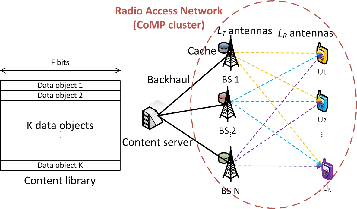
Figure 1: Architecture of cached MIMO interference networks.

Consider a cached MIMO interference network with $N$ BS-user pairs, as illustrated in Fig. 1. Each BS has $L_{T}$ antennas and each user has $L_{R}$ antennas. Each BS has transmit power $P$ and a cache of $L_{C}F$ bits. There is a content server providing a content library $\mathcal{K}$ that contains $K$ data objects, where each data object has $F$ bits. The users request data objects from the content server via a radio access network (RAN). Each BS in the RAN is connected to the content server via a backhaul. The content server also serves as a central control node responsible for resource control of all the BSs. Such a cluster architecture appears in practical LTE networks.

For convenience, let $\mathcal{B}$ denote the set of BSs, $\mathcal{U}$ denote the set of users, $\mathcal{M}=\mathcal{B}\cup\mathcal{U}$ denote the set of all nodes, and $g$ denote the content server. The serving BS of user $j\in\mathcal{U}$ is denoted as $n_{j}$ and the associated user of BS $n\in\mathcal{B}$ is denoted as $j_{n}$. A user always sends its data object request to its serving BS. However, it may receive the requested data object from only the serving BS or from all BSs, depending on the PHY mode, as will be elaborated in the next subsection.

Time is partitioned into frames indexed by $i$, and each frame consists of $T$ time slots indexed by $t$, as illustrated in Fig. 3. Each time slot corresponds to a channel coherence time and the fast-timescale resource control variables (mode selection and rate allocation) are updated at the beginning of each time slot. On the other hand, the slow-timescale resource control variables (cache content placement control) are updated at the beginning of each frame. Unless otherwise specified, $t$ is used to index a time slot in frame $i$, i.e., $t\in\left[1+(i-1)T,iT\right]$ and $i=\left\lceil\frac{t}{T}\right\rceil$.

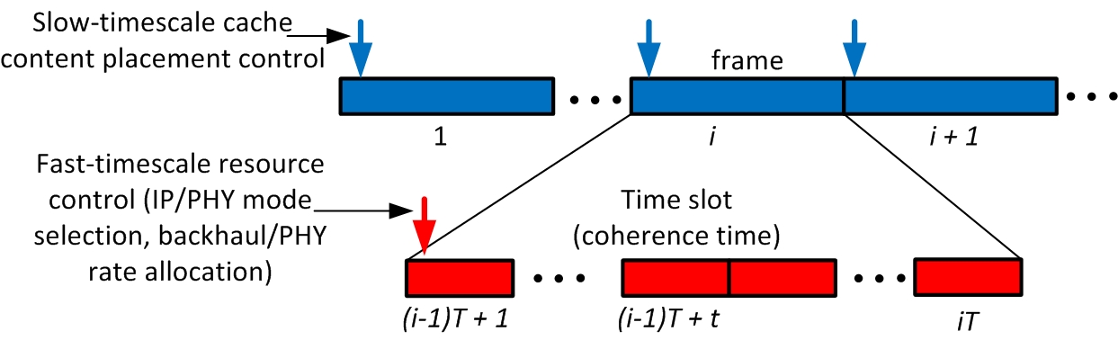
Figure 2: Illustration of the time slot and frame.

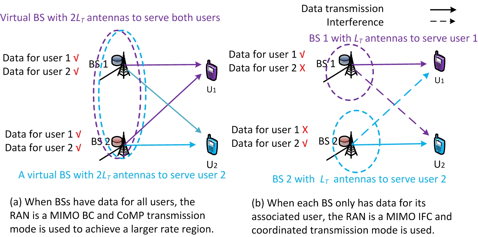
Figure 3: Illustration of the dual-mode PHY.

II-B Dual-Mode Physical Layer Model

We assume that the content server has knowledge of the global channel state information (CSI) $\boldsymbol{H}\left(t\right)=\left\{\boldsymbol{H}_{jn}\left(t\right),\forall j\in\mathcal{U},n\in\mathcal{B}\right\}$ of the RAN, where $\boldsymbol{H}_{jn}\left(t\right)\in\mathbb{C}^{L_{R}\times L_{T}}$ is the channel matrix between the $n$-th BS and the $j$-th user at the $t$-th time slot, and $\boldsymbol{H}\left(t\right)$ is quasi-static within a time slot and i.i.d. between time slots. The time index $t$ in $\boldsymbol{H}\left(t\right)$ will be omitted when there is no ambiguity. There are two PHY modes, as elaborated below.

CoMP transmission mode (PHY mode A): In this mode, the BSs can form a virtual transmitter and cooperatively send some data to all users. In this case, the RAN is a virtual MIMO broadcast channel (BC), as illustrated in Fig. 3-(a). Specifically, let $B_{j}\left(t\right)$ denote the data scheduled for delivery to user $j$ at time slot $t$. In CoMP mode, $B_{j}\left(t\right)$ must be available at all BSs. The amount of scheduled data $\left|B_{j}\left(t\right)\right|$ (measured by the number of data objects) is limited by the data rate of the CoMP mode PHY, i.e., $\left|B_{j}\left(t\right)\right|=c_{j}^{A}\left(t\right)$, where $c_{j}^{A}\left(t\right)$ (data objects/slot) is the data rate of user $j$ under CoMP mode with CSI $\boldsymbol{H}\left(t\right)$. To achieve the data rate $c_{j}^{A}\left(t\right)$, a coding scheme $\beta_{nj}^{A}:\left\{0,1\right\}^{c_{j}^{A}\left(t\right)F}\rightarrow\mathbb{C}^{L_{T}\times N_{c}}$ is applied at BS $n,\forall n\in\mathcal{B}$ for the data $B_{j}\left(t\right)$ requested by user $j$, which maps $B_{j}\left(t\right)$ to a codeword: $\boldsymbol{X}_{nj}^{A}\left(t\right)=\beta_{nj}^{A}\left(B_{j}\left(t\right)\right)\in\mathbb{C}^{L_{T}\times N_{c}}$, where $N_{c}$ is the number of data symbol vectors per time slot. The signal $\boldsymbol{X}_{n}^{A}\left(t\right)$ transmitted from BS $n$ in the $t$-th time slot is a superposition of the codewords for all users: $\boldsymbol{X}_{n}^{A}\left(t\right)=\sum_{j\in\mathcal{U}}\boldsymbol{X}_{nj}^{A}\left(t\right)\in\mathbb{C}^{L_{T}\times N_{c}}$, where each column vector in $\boldsymbol{X}_{n}^{A}\left(t\right)$ is transmitted from the $L_{T}$ antennas during a symbol period in time slot $t$. Moreover, $\boldsymbol{X}_{n}^{A}\left(t\right)$ satisfies a power constraint $\mathrm{Tr}\left(\boldsymbol{X}_{n}^{A}\left(t\right)\left(\boldsymbol{X}_{n}^{A}\left(t\right)\right)^{H}\right)/N_{c}\leq P$. The received signal at user $j$ in the $t$-th time slot is

$$\boldsymbol{Y}_{j}\left(t\right)=\sum_{n\in\mathcal{B}}\boldsymbol{H}_{jn}\left(t\right)\boldsymbol{X}_{n}^{A}\left(t\right)+\boldsymbol{Z}_{j}\left(t\right)\in\mathbb{C}^{L_{R}\times N_{c}},$$ (1)

where $\boldsymbol{Z}_{j}\left(t\right)$ is the additive white Gaussian noise (AWGN). The rate $c_{j}^{A}\left(t\right)$ is achievable at the $t$-th time slot if user $j$ can decode the scheduled data $B_{j}\left(t\right)$ with vanishing error probability as $N_{c}\rightarrow\infty$. The set of achievable rate vectors $\boldsymbol{c}^{A}\left(t\right)=\left[c_{j}^{A}\left(t\right)\right]_{j\in\mathcal{U}}\in\mathbb{R}_{+}^{N}$ forms the capacity region $C^{A}\left(\boldsymbol{H}\left(t\right)\right)\in\mathbb{R}_{+}^{N}$ under the CoMP mode.

Coordinated transmission mode (PHY mode B): In this case, user $j$ can only be served by the serving BS $n_{j}$ and the RAN is a MIMO interference channel (IFC), as illustrated in Fig. 3-(b). Similarly, we have $\left|B_{j}\left(t\right)\right|=c_{j}^{B}\left(t\right)$, where $c_{j}^{B}\left(t\right)$ (data objects/slot) is the data rate of user $j$ under coordinated mode with CSI $\boldsymbol{H}\left(t\right)$. To achieve the data rate $c_{j}^{B}\left(t\right)$, a coding scheme $\beta_{j}^{B}:\left\{0,1\right\}^{c_{j}^{B}\left(t\right)F}\rightarrow\mathbb{C}^{L_{T}\times N_{c}}$ is applied at BS $j_{n}$ to map $B_{j}\left(t\right)$ to a codeword: $\boldsymbol{X}_{j}^{B}\left(t\right)=\beta_{j}^{B}\left(B_{j}\left(t\right)\right)\in\mathbb{C}^{L_{T}\times N_{c}}$, where $\boldsymbol{X}_{j}^{B}\left(t\right)$ satisfies a power constraint $\mathrm{Tr}\left(\boldsymbol{X}_{j}^{B}\left(t\right)\left(\boldsymbol{X}_{j}^{B}\left(t\right)\right)^{H}\right)/N_{c}\leq P$. The received signal at user $j$ in the $t$-th time slot is

$$\boldsymbol{Y}_{j}\left(t\right)=\sum_{j^{{}^{\prime}}\in\mathcal{K}}\boldsymbol{H}_{jn_{j^{{}^{\prime}}}}\left(t\right)\boldsymbol{X}_{j^{{}^{\prime}}}^{B}\left(t\right)+\boldsymbol{Z}_{j}\left(t\right)\in\mathbb{C}^{L_{R}\times N_{c}}.$$ (2)

The rate $c_{j}^{B}\left(t\right)$ at the $t$-th time slot is achievable if the user $j$ can decode the scheduled data $B_{j}\left(t\right)$ with vanishing error probability as $N_{c}\rightarrow\infty$. The set of achievable rate vectors $\boldsymbol{c}^{B}\left(t\right)=\left[c_{j}^{B}\left(t\right)\right]_{j\in\mathcal{U}}\in\mathbb{R}_{+}^{N}$ forms the capacity region $C^{B}\left(\boldsymbol{H}\left(t\right)\right)\in\mathbb{R}_{+}^{N}$ under the coordinated transmission mode.

There exist many CoMP/coordinated transmission schemes (coding schemes $\left\{\beta_{nj}^{A}\right\}/\left\{\beta_{j}^{B}\right\}$). In this paper, we do not restrict the PHY to be any specific CoMP/coordinated transmission scheme but consider an abstract PHY model represented by the capacity regions $C^{A}\left(\boldsymbol{H}\right)$ and $C^{B}\left(\boldsymbol{H}\right)$. Note that $C^{A}\left(\boldsymbol{H}\right)$ and $C^{B}\left(\boldsymbol{H}\right)$ depend on the transmit power $P$ at each BS. Moreover, we have $C^{B}\left(\boldsymbol{H}\right)\subseteq C^{A}\left(\boldsymbol{H}\right)$ according to the definitions of $C^{A}\left(\boldsymbol{H}\right)$ and $C^{B}\left(\boldsymbol{H}\right)$.

In the following, we use linear precoding to illustrate the dual mode physical layer.

CoMP Mode under linear precoding: In this mode, the $N$ users are served using CoMP linear precoding between the BSs. The received signal for user $j$ can be expressed as:

$$\boldsymbol{y}_{j}=\widetilde{\boldsymbol{H}}_{j}\boldsymbol{V}_{j}^{A}\boldsymbol{x}_{j}^{A}+\sum_{j^{{}^{\prime}}\neq j}\widetilde{\boldsymbol{H}}_{j}\boldsymbol{V}_{j^{{}^{\prime}}}^{A}\boldsymbol{x}_{j^{{}^{\prime}}}^{A}+\boldsymbol{z}_{j},$$ (3)

where $\widetilde{\boldsymbol{H}}_{j}=\left[\boldsymbol{H}_{j1},...,\boldsymbol{H}_{jN}\right]\in\mathbb{C}^{L_{R}\times NL_{T}}$ is the composite channel matrix between all the BSs and user $j$; $\boldsymbol{x}_{j}^{A}\in\mathbb{C}^{d_{j}^{A}}\sim\mathcal{CN}\left(0,\boldsymbol{I}\right)$ and $d_{j}^{A}$ are respectively the data vector and the number of data streams for user $j$; $\boldsymbol{V}_{j}^{A}\in\mathbb{C}^{NL_{T}\times d_{j}^{A}}$ is the composite precoding matrix for user $j$, and $\boldsymbol{z}_{j}$ is the AWGN. For given CSI $\boldsymbol{H}$ and precoding matrices $\boldsymbol{V}^{A}=\left\{\boldsymbol{V}_{j}^{A}:\forall j\right\}$, the data rate (bps) of user $j$ under the CoMP mode is [14]

$$c_{j}^{A}\left(\boldsymbol{H},\boldsymbol{V}^{A}\right)=B_{W}\textrm{log}_{2}\left|\boldsymbol{I}+\widetilde{\boldsymbol{H}}_{j}\boldsymbol{V}_{j}^{A}\boldsymbol{V}_{j}^{AH}\widetilde{\boldsymbol{H}}_{j}^{H}\widetilde{\mathbf{\Omega}}_{j}^{-1}\right|,$$ (4)

where $B_{W}$ is the channel bandwidth, and $\widetilde{\mathbf{\Omega}}_{j}=\boldsymbol{I}+\sum_{j^{{}^{\prime}}\neq j}\widetilde{\boldsymbol{H}}_{j}\boldsymbol{V}_{j^{{}^{\prime}}}^{A}\boldsymbol{V}_{j^{{}^{\prime}}}^{H}\widetilde{\boldsymbol{H}}_{j}^{H}$ is the interference-plus-noise covariance matrix of user $j$.

Coordinated mode under linear precoding: In this mode, the user $j$ can only be served by BS $j$ using coodinated linear precoding. The received signal for user $j$ can be expressed as:

$$\boldsymbol{y}_{j}=\boldsymbol{H}_{jn_{j}}\boldsymbol{V}_{j}^{B}\boldsymbol{x}_{j}^{B}+\sum_{j^{{}^{\prime}}\neq j}\boldsymbol{H}_{jn_{j^{{}^{\prime}}}}\boldsymbol{V}_{j^{{}^{\prime}}}^{B}\boldsymbol{x}_{j^{{}^{\prime}}}^{B}+\boldsymbol{z}_{j},$$ (5)

where $\boldsymbol{x}_{j}^{B}\in\mathbb{C}^{d_{j}^{B}}\sim\mathcal{CN}\left(0,\boldsymbol{I}\right)$ and $d_{j}^{B}$ are respectively the data vector and the number of data streams for user $j$; and $\boldsymbol{V}_{j}^{B}\in\mathbb{C}^{L_{T}\times d_{j}^{B}}$ is the precoding matrix for user $j$. For given CSI $\boldsymbol{H}$ and precoding matrices $\boldsymbol{V}^{B}=\left\{\boldsymbol{V}_{j}^{B}:\forall j\right\}$, the data rate of user $j$ under coordinated mode is [14]

$$c_{j}^{B}\left(\boldsymbol{H},\boldsymbol{V}^{B}\right)=B_{W}\textrm{log}_{2}\left|\boldsymbol{I}+\boldsymbol{H}_{jn_{j}}\boldsymbol{V}_{j}^{B}\boldsymbol{V}_{j}^{BH}\boldsymbol{H}_{jn_{j}}^{H}\mathbf{\Omega}_{j}^{-1}\right|,$$ (6)

where $\mathbf{\Omega}_{j}=\boldsymbol{I}+\sum_{j^{{}^{\prime}}\neq j}\boldsymbol{H}_{jn_{j^{{}^{\prime}}}}\boldsymbol{V}_{j^{{}^{\prime}}}^{B}\boldsymbol{V}_{j^{{}^{\prime}}}^{BH}\boldsymbol{H}_{jn_{j^{{}^{\prime}}}}^{H}$ is the interference-plus-noise covariance matrix.

III Mixed-Timescale Online PHY Caching and Content Delivery Scheme

III-A Slow-Timescale Online PHY Caching Scheme

In the proposed online PHY caching scheme, the cached data objects at each BS are updated once every frame ($T$ time slots), as illustrated in Fig. 3. Since the local popularity variations at each BS usually change at a timescale much slower than the instantaneous CSI (slot interval), in practice, we may choose $T\gg 1$ to reduce the cache content placement cost without losing the ability to track microscopic spatial and temporary popularity variations.

Let $s_{n}^{k}(i)\in\left\{0,1\right\}$ denote the cache state of data object $k$ at BS $n$, where $s_{n}^{k}(i)=1$ means that data object $k$ is in the cache of BS $n$ at frame $i$ and $s_{n}^{k}(i)=0$ means the opposite. The cache placement control action at the beginning of the $i$-th frame is denoted by $\left\{p_{n}^{k}(i)\in\left\{-1,0,1\right\},\forall n,k\right\}$, where $p_{n}^{k}(i)=-1$ and $p_{n}^{k}(i)=1$ mean that the data object $k$ is removed from and added to the cache of BS $n$ at the beginning of the $i$-th frame respectively, and $p_{n}^{k}(i)=0$ means that the cache state is unchanged. Note that there is no need to add an existing data object to the cache or remove a non-existing data object, i.e.,

$$p_{n}^{k}(i) \neq 1,\textrm{when }s_{n}^{k}(i-1)=1.$$

$$p_{n}^{k}(i) \neq-1,\textrm{when }s_{n}^{k}(i-1)=0.$$ (7)

As such, the cache state dynamics is

$$s_{n}^{k}(i)=s_{n}^{k}(i-1)+p_{n}^{k}(i),\forall n\in\mathcal{B},k\in\mathcal{K}.$$ (8)

The cache placement control action $\left\{p_{n}^{k}(i)\right\}$ must satisfy the following cache size constraint:

$$\sum_{k\in\mathcal{K}}s_{n}^{k}(i)\leq L_{C},\forall i,\forall n\in\mathcal{B}.$$ (9)

Let $\boldsymbol{s}\left(i\right)=\left\{s_{n}^{k}(i),\forall n\in\mathcal{B},k\in\mathcal{K}\right\}$ denote the aggregate cache state. When $p_{n}^{k}(i)=1$, BS $n$ needs to obtain data object $k$ from the backhaul, which induces some cache content placement cost. To accommodate the traffic caused by cache content placement, the available backhaul capacity $R$ (data objects/slot) at each BS is divided into a data sub-channel and a control sub-channel as $R=R_{c}+R_{d}$, where the data sub-channel with rate $R_{d}$ is used for transmitting the data objects requested by users, and the control sub-channel is used for transmitting the data objects induced by the cache placement control and other control signalings. The cache content placement cost for BS $n$ to cache data object $k$ at frame $i$ is $\Gamma_{n}^{k}(i)=\gamma\mathbf{1}{}_{\{p_{n}^{k}(i)=1\}}$, where $\mathbf{1}$ denotes the indication function, and $\gamma$ is the price of fetching one data object using the control sub-channel. The total cost function at frame $i$ is

$$\Gamma(i)=\sum_{n\in\mathcal{B},k\in\mathcal{K}}\Gamma_{n}^{k}(i)=\sum_{n\in\mathcal{B},k\in\mathcal{K}}\gamma\mathbf{1}{}_{\{p_{n}^{k}(i)=1\}},$$ (10)

and the average cache content placement cost is

$$\overline{\Gamma}=\limsup_{J\rightarrow\infty}\frac{1}{J}\sum_{i=1}^{J}\mathbb{E}\left[\Gamma\left(i\right)\right].$$ (11)

III-B Fast-Timescale Dual-Mode Content Delivery Scheme

We consider a dual-mode content delivery scheme which can support the CoMP to enhance the capacity of the RAN. Specifically, each data object is divided into $D$ data chunks, and each data chunk is allocated a unique ID. The content delivery operates at the level of data chunks using two types of packets: Interest Packets (IPs) and Data Packets (DPs). To request a data chunk, a user sends out an IP, which carries the ID of the data chunk, to the content server via its serving BS. Hence, a request for a data object consists of a sequence of IPs which request all the data chunks of the object.

For each IP from user $j$, the content server determines its mode (coordinated mode IP or CoMP mode IP) according to an IP mode selection policy that will be elaborated in Section IV-C. If it is marked as a CoMP Mode IP, the corresponding DP will be delivered to all BSs and stored in the CoMP mode data buffer at each BS. If it is marked as a coordinated mode IP, the corresponding DP will be delivered to the serving BS $n_{j}$ only, and stored in a coordinated mode data buffer at BS $n_{j}$. At each time slot, the content server also needs to determine the PHY mode $M_{a}\left(t\right)\in\left\{0,1\right\}$ according to the PHY mode selection policy elaborated in Section IV-C. If $M_{a}\left(t\right)=0$ ($M_{a}\left(t\right)=1$), the BSs will employ the coordinated (CoMP) mode to transmit some data from the coordinated (CoMP) mode data buffers to the users.

The dual-mode content delivery has four components.

Component 1 (IP mode selection at content server): Let $Da_{j}^{k}(t)$ denote the number of IPs of data object $k$ received by the content server from user $j$ at time slot $t$, where $a_{j}^{k}(t)$ can be interpreted as the instantaneous arrival rate of IPs in the unit of data object/slot since each data object corresponds to $D$ IPs. The content server will mark all these $Da_{j}^{k}(t)$ IPs using the same IP mode, denoted by $m_{j}^{k}\left(t\right)\in\left\{0,1\right\}$.

Component 2 (coordinated mode DPs’ delivery to each BS): If $m_{j}^{k}\left(t\right)=0$, the corresponding $Da_{j}^{k}(t)$ DPs are called coordinated mode DPs, which will be delivered to the serving BS $n_{j}$ only. Specifically, if BS $n_{j}$ has data object $k$ in the local cache ($s_{n_{j}}^{k}\left(i\right)=1$), it creates $Da_{j}^{k}(t)$ DPs containing the requested data chunks indicated by the $Da_{j}^{k}(t)$ IPs. Otherwise, the content server will create the requested $Da_{j}^{k}(t)$ DPs and store them in the $n_{j}$-th data buffer with queue length $Q_{gn_{j}}$ at the content server. These will be sent to BS $n_{j}$ via backhaul when they become the head-of-the-queue DPs. In both cases, after obtaining the $Da_{j}^{k}(t)$ DPs, BS $n_{j}$ will store them in the coordinated mode data buffer $Q_{n_{j}j}^{B}$.

Component 3 (CoMP mode DPs’ delivery to each BS): If $m_{j}^{k}\left(t\right)=1$, the corresponding $Da_{j}^{k}(t)$ DPs are called CoMP mode DPs, which will be delivered to all BSs. For any $n\in\mathcal{B}$, if BS $n$ has data object $k$ in the local cache ($s_{n}^{k}\left(i\right)=1$), it creates the requested $Da_{j}^{k}(t)$ DPs. Otherwise, the content server will create the requested $Da_{j}^{k}(t)$ DPs and store them in the $n$-th data buffer $Q_{gn}$ at the content server. These will be sent to BS $n$ via backhaul when they become the head-of-the-queue DPs. In both cases, after obtaining the $Da_{j}^{k}(t)$ DPs, BS $n$ will store the $Da_{j}^{k}(t)$ DPs in the $j$-th CoMP mode data buffer $Q_{nj}^{A}$.

Component 4 (PHY mode determination at content server): The content server determines the PHY mode $M_{a}\left(t\right)$. If $M_{a}\left(t\right)=0$, coordinated transmission mode will be used to send the data in $Q_{nj_{n}}^{B}$ to user $j_{n}$, $\forall j_{n}\in\mathcal{U}$, at rate $c_{j_{n}}^{B}\left(t\right)$ (data objects/slot). If $M_{a}\left(t\right)=1$, CoMP transmission mode will be used to send the data in $Q_{nj}^{A}$ to user $j$, $\forall j\in\mathcal{U}$, at rate $c_{j}^{A}\left(t\right)$. Let $\boldsymbol{c}^{B}\left(t\right)=\left[c_{j}^{B}\left(t\right)\right]_{j\in\mathcal{U}}\in\mathbb{R}_{+}^{N}$ and $\boldsymbol{c}^{A}\left(t\right)=\left[c_{j}^{A}\left(t\right)\right]_{j\in\mathcal{U}}\in\mathbb{R}_{+}^{N}$ denote the PHY rate allocation for the coordinated and CoMP modes respectively.

III-C Data Packet Queue Dynamics

The dynamics of the queue $Q_{gn}$ at the content server is

$$Q_{gn}\left(t+1\right)=\left(Q_{gn}(t)-c_{ng}(t)\right)^{+}+b_{n}(t),$$ (12)

where $b_{n}(t)=\sum_{k\in\mathcal{K}}\overline{s}_{n}^{k}\left(i\right)\left(\sum_{j\in\mathcal{U}}m_{j}^{k}\left(t\right)a_{j}^{k}(t)+\overline{m}_{j_{n}}^{k}\left(t\right)a_{j_{n}}^{k}(t)\right)$ is the arrival rate of $Q_{gn}\left(t\right)$, $\overline{s}_{n}^{k}\left(i\right)=\boldsymbol{1}_{s_{n}^{k}\left(i\right)=0}$, $\overline{m}_{j}^{k}\left(t\right)=\boldsymbol{1}_{m_{j}^{k}\left(t\right)=0}$, and $c_{ng}(t)$ is the allocated transmission rate of DPs from the content server to BS $n$ during time slot $t$. Let $Db_{nj_{n}}^{B}(t)$ ($Db_{nj}^{A}(t)$) denote the number of coordinated mode DPs of user $j_{n}$ (CoMP mode IPs of user $j$) obtained at BS $n$ from either the backhaul or the local cache. The dynamics of the queues at BS $n$ are

$$Q_{nj_{n}}^{B}\left(t+1\right) =\left(Q_{nj_{n}}^{B}\left(t\right)-\overline{M}_{a}\left(t\right)c_{j_{n}}^{B}\left(t\right)\right)^{+}+b_{nj_{n}}^{B}(t),$$

$$Q_{nj}^{A}\left(t+1\right) =Q_{nj}^{A}\left(t\right)-\min\left(M_{a}\left(t\right)c_{j}^{A}\left(t\right),\check{Q}_{j}^{A}\left(t\right)\right)+b_{nj}^{A}(t),$$ (13)

where $\overline{M}_{a}\left(t\right)=\boldsymbol{1}_{M_{a}\left(t\right)=0}$ and $\check{Q}_{j}^{A}\left(t\right)=\min_{n}Q_{nj}^{A}\left(t\right)$. Note that the queue length is measured using the number of data objects and the arrival rate is measured in data objects/slot because the proposed resource control framework operates at the data object level.

IV Dual-Mode-VIP-based Resource Control

In the proposed scheme, the slow-timescale cache content placement policy $\left\{p_{n}^{k}(i)\right\}$ is adaptive to the local popularity information at each node. The fast-timescale controls include the IP mode selection $\left\{m_{j}^{k}\left(t\right)\right\}$, backhaul rate allocation $\left\{c_{ng}(t)\right\}$, PHY mode selection $M_{a}\left(t\right)$, and PHY rate allocation $\left\{\boldsymbol{c}^{A}\left(t\right),\boldsymbol{c}^{B}\left(t\right)\right\}$, which are adaptive to the cache state $\left\{s_{n}^{k}(i)\right\}$ and global CSI $\boldsymbol{H}\left(t\right)$. However, the local popularity information is unavailable in the actual plane (network) due to interest collapsing and suppression, which refers to the operation that multiple unsatisfied requests (IPs) for the same DP at a node will be aggregated into a single IP [9]. This is good for efficiency, but also bad since we lose track of the actual expressed demand once the suppression happens. To overcome this challenge, we consider a dual-mode VIP framework, which creates a virtual plane (network) in which multiple interests are not suppressed via the introduction of Virtual Interest Packets (VIPs), to keep a sufficient statistic for the design of resouce control algorithm. As such, resource control algorithms operating in the virtual plane can take advantage of local popularity information on network demand (as represented by the VIP counts), which is unavailable in the actual plane. Moreover, this dual-mode-VIP-based approach also reduces the implementation complexity of the VIP algorithm in the virtual plane considerably (as compared with operating on DPs/IPs in the actual plane).

IV-A Transformation to a Virtual Network

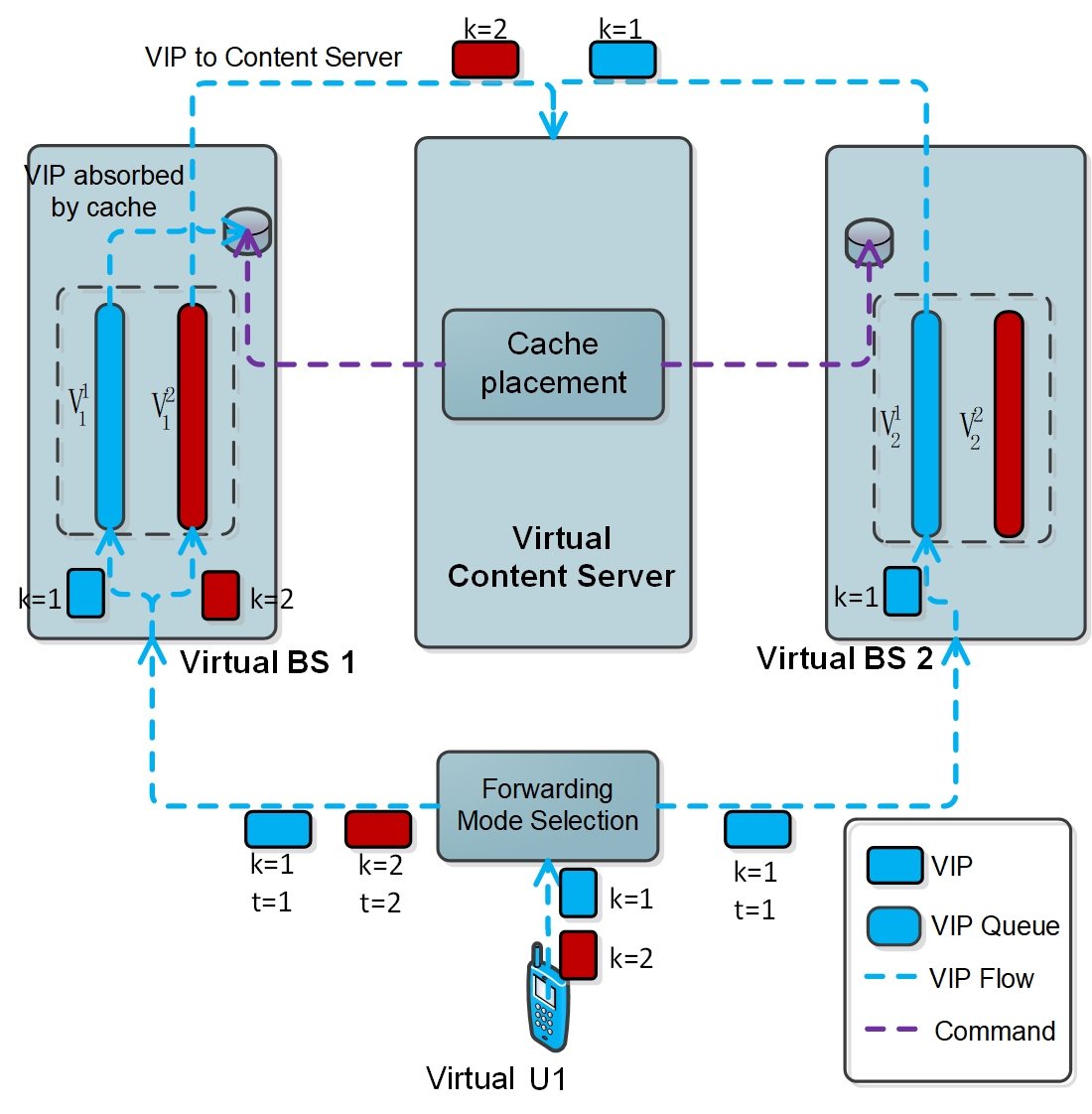
Figure 4: Illustration of the VIP flow in the virtual network. In this example, user 1 requests data object 1 at time slot 1 and data object 2 at time slot 2. BS 1’s cache contains data object 1 and BS 2’s cache contains data object 2. The forwarding mode is CoMP mode at time slot 1, and coordinated mode at time slot 2. Therefore, the blue VIP with ID $k=1$ is forwarded to both BSs, and the red VIP with ID $k=2$ is forwarded to BS 1 only. Moreover, BS 1 (2) forwards the red (blue) VIP associated with data object 2 (1) to content server since data object 2 (1) is not stored at BS1 (2).

The dual-mode VIP framework relies on the concept of VIPs flowing over a virtual network, as illustrated in Fig. 4. The virtual network is simulated at the content server and it has exactly the same topology, cache state $\left\{s_{n}^{k}(i)\right\}$ and global CSI $\boldsymbol{H}\left(t\right)$ as the actual network. Each virtual node $m\in\mathcal{N}$ maintains a VIP queue $V_{m}^{k}(t)$ for each data object $k$, which is implemented as a counter in the content server. The VIP queue $V_{m}^{k}(t)$ captures the local popularity at each (virtual) node, and the set of all VIP queues $\mathbf{V}(t)=\left\{V_{m}^{k}(t),\forall m\in\mathcal{M},k\in\mathcal{K}\right\}$ captures microscopic popularity variations. Initially, all VIP queues are set to 0, i.e., $V_{m}^{k}(1)=0,\forall m\in\mathcal{M},k\in\mathcal{K}$. As the content server receives data object requests (IPs requesting the starting chunk of data objects) from users, the corresponding VIP queues $V_{j}^{k}(t),j\in\mathcal{U}$ are incremented accordingly. After some number of VIPs in $V_{j}^{k}(t),j\in\mathcal{U}$ have been “forwarded” to the virtual BSs (in the virtual network), the VIP queues $V_{j}^{k}(t),j\in\mathcal{U}$ are decreased and the VIP queues $V_{n}^{k}(t),n\in\mathcal{B}$ are increased by the same number accordingly. Similarly, after some number of VIPs in $V_{n}^{k}(t),n\in\mathcal{B}$ have been “forwarded” to the virtual content server (content source) and local cache, the VIP queues $V_{n}^{k}(t),n\in\mathcal{B}$ are decreased by the same number accordingly. Specifically, in the virtual network, there are two modes for “forwarding” the VIPs from the virtual users to virtual BSs, corresponding to the two PHY modes in the actual plane.

In the CoMP forwarding mode, VIPs in $V_{j}^{k}(t)$ are forwarded to all virtual BSs, and thus at time $t+1$, the VIP queues become

$$V_{j}^{k}(t+1) =\left(V_{j}^{k}(t)-\mu_{j}^{Ak}(t)\right)^{+}+A_{j}^{k}(t),$$

$$V_{n}^{k}(t+1) =\left(\left(V_{n}^{k}(t)-\mu_{ng}^{k}(t)\right)^{+}+\sum_{j\in\mathcal{U}}\mu_{j}^{Ak}(t)-r_{n}s_{n}^{k}\left(i\right)\right)^{+}$$ (14)

$\forall j\in\mathcal{U},n\in\mathcal{B}$, where $A_{j}^{k}(t)$ is the number of exogenous data object request arrivals at the VIP queue $V_{j}^{k}(t)$ during slot $t$, $\mu_{j}^{Ak}(t)$ is the allocated transmission rate of VIPs for data object $k$ from virtual user $j$ to all virtual BSs during time slot $t$ with CoMP forwarding mode, $\mu_{ng}^{k}(t)$ is the allocated transmission rate of VIPs for data object $k$ from virtual BS $n$ to the virtual content server during time slot $t$, and $r_{n}$ is the maximum rate (in data objects/slot) at which BS $n$ can produce copies of cached object $k$ (e.g., the maximum rate $r_{n}$ may reflect the I/O rate of the storage disk). On the other hand, in the coordinated forwarding mode, VIPs in $V_{j}^{k}(t)$ are “forwarded” to the serving virtual BS $n_{j}$ only, and thus at time $t+1$, the VIP queues become

$$V_{j}^{k}(t+1) =\left(V_{j}^{k}(t)-\mu_{j}^{Bk}(t)\right)^{+}+A_{j}^{k}(t),$$

$$V_{n}^{k}(t+1) =\left(\left(V_{n}^{k}(t)-\mu_{ng}^{k}(t)\right)^{+}+\mu_{j_{n}}^{Bk}(t)-r_{n}s_{n}^{k}\left(i\right)\right)^{+},$$ (15)

$\forall j\in\mathcal{U},n\in\mathcal{B}$, where $\mu_{j}^{Bk}(t)$ is the allocated transmission rate of VIPs for data object $k$ from virtual user $j$ to virtual BS $n_{j}$ during time slot $t$ with coordinated forwarding mode.

Combining the above two cases, the VIP queue dynamics can be expressed in a compact form:

$$V_{j}^{k}(t+1) =\left(V_{j}^{k}(t)-\mu_{j}^{Ak}(t)M\left(t\right)-\mu_{j}^{Bk}(t)\overline{M}\left(t\right)\right)^{+}+A_{j}^{k}(t)$$

$$V_{n}^{k}(t+1) =\bigg{(}\left(V_{n}^{k}(t)-\mu_{ng}^{k}(t)\right)^{+}+\sum_{j\in\mathcal{U}}\mu_{j}^{Ak}(t)M\left(t\right)$$

$$+\mu_{j_{n}}^{Bk}(t)\overline{M}\left(t\right)-r_{n}s_{n}^{k}\left(i\right)\bigg{)}^{+},\forall j\in\mathcal{U},n\in\mathcal{B},k\in\mathcal{K}$$ (16)

where $M\left(t\right)\in\left\{0,1\right\}$ is the forwarding mode at time slot $t$ in the virtual plane ($M\left(t\right)=0$ stands for the coordinated forwarding mode and $M\left(t\right)=1$ stands for the CoMP forwarding mode), and $\overline{M}\left(t\right)=\boldsymbol{1}_{M\left(t\right)=0}$.

In Table I, we list the key notations in the actual network and the corresponding notations in the virtual network for easy reference.

Notations in the actual network	Notations in the virtual network
PHY mode $M_{a}$ and IP modes $\left\{m_{j}^{k}\right\}$	Forwarding mode $M$
PHY rates $\left\{\boldsymbol{c}^{A},\boldsymbol{c}^{B}\right\}$	Forwarding rates between BSs and users $\left\{\boldsymbol{\mu}^{A},\boldsymbol{\mu}^{B}\right\}$
Backhaul rates $\left\{c_{ng}\right\}$	Forwarding rates between BSs and server $\left\{\mu_{ng}^{k}\right\}$
DP queues $\left\{Q_{nj}^{A},Q_{nj_{n}}^{B},Q_{gn}\right\}$	VIP queues$\left\{V_{n}^{k},V_{j}^{k}\right\}$
IPs arrival rates $\left\{a_{j}^{k}\right\}$	VIPs arrival rates $\left\{A_{j}^{k}\right\}$
Stability region $\Lambda_{c}$	VIP stability region $\Lambda_{v}$

Table I: Key notations in the actual and virtual networks.

IV-B Mixed-Timescale Resource Control in Virtual Network

A mixed-timescale resource control algorithm determines the slow-timescale cache content placement policy $\left\{p_{n}^{k}(i)\right\}$ and the fast-timescale policies in the virtual network, aiming at solving the following problem:

$$\min_{\left\{p_{n}^{k}(i),M\left(t\right),\mu_{j}^{Ak}(t),\mu_{j}^{Bk}(t),\mu_{ng}^{k}(t)\right\}}\limsup_{t\rightarrow\infty}\frac{1}{t}\sum_{\tau=1}^{t}\sum_{m\in\mathcal{M},k\in\mathcal{K}}\mathbb{E}\left[V_{m}^{k}(\tau)\right]+W\limsup_{J\rightarrow\infty}\frac{1}{J}\sum_{i=1}^{J}\mathbb{E}\left[\Gamma\left(i\right)\right],$$

$$\text{s.t.}\sum_{k\in\mathcal{K}}s_{n}^{k}(i)\leq B_{C},\forall n\in\mathcal{B},\forall i,$$

$$\sum_{k\in\mathcal{K}}\mu_{ng}^{k}(t)\leq R_{d},\forall n;\boldsymbol{\mu}^{A}\left(t\right)\in C^{A}\left(\boldsymbol{H}\right);\boldsymbol{\mu}^{B}\left(t\right)\in C^{B}\left(\boldsymbol{H}\right),\forall t,$$ (17)

where the objective function is a weighted sum of the total average VIP queue length and average cache placement cost, $W$ is a price factor which can be used to control the tradeoff between the stability (measured by the total average VIP queue length) and average cache placement cost. However, it is difficult to directly solve this problem. Therefore, we resort to the Lyapunov optimization framework [11, 12] and approximately solve this problem by minimizing a mixed-timescale drift-plus-penalty as follows.

IV-B1 Slow-Timescale Cache Content Placement Solution

Define $\mathcal{L}(\mathbf{V}(t))\triangleq\sum_{n\in\mathcal{N},k\in\mathcal{K}}\left(V_{n}^{k}(t)\right)^{2}$ as the Lyapunov function, which is a measure of unsatisfied requests in the network. The cache content placement $\left\{p_{n}^{k}(i)\right\}$ is designed to minimize the $T$-step VIP-drift-plus-penalty defined as

$$\Delta_{T}\left(i\right)\triangleq\mathbb{E}\left[\mathcal{L}(\mathbf{V}(t_{0}^{i}+T))-\mathcal{L}(\mathbf{V}(t_{0}^{i}))|\boldsymbol{X}(t_{0}^{i})\right]$$

$$+W\mathbb{E}\left[\sum_{n\in\mathcal{B},k\in\mathcal{K}}\gamma 1_{\{p_{n}^{k}(i)=1\}}|\boldsymbol{X}(t_{0}^{i})\right],$$ (18)

where $t_{0}^{i}$ is the starting time slot of the $i$-th frame, and $\boldsymbol{X}(t_{0}^{i})=\left[\mathbf{V}(t_{0}^{i})\,\boldsymbol{s}(i-1)\right]$ is the observed system state at the beginning of the frame. Intuitively, if the first term in $\Delta_{T}\left(i\right)$ is negative, the VIP lengths tend to decrease. On the other hand, the second term in $\Delta_{T}\left(i\right)$ is the weighted cache content placement cost, and $W$ is a price factor. Therefore, minimizing $\Delta_{T}\left(i\right)$ helps to strike a balance between stability and cost reduction. Following a similar analysis to that in the proof of Lemma 3 in [15], we obtain an upper bound of $\Delta_{T}\left(i\right)$.

Theorem 1 ($T$-step Drift-Plus-Penalty Upper Bound).

An upper bound of $\Delta_{T}\left(i\right)$ is $\widetilde{\Delta}_{T}\left(i\right)\triangleq\mathbb{E}\left[\Delta_{T}^{U}\left(i\right)|\boldsymbol{X}(t_{0}^{i})\right]$, where

$$\Delta_{T}^{U}\left(i\right)=W\sum_{n\in\mathcal{B},k\in\mathcal{K}}\gamma 1_{\{p_{n}^{k}(i)=1\}}+\overline{\Delta}$$

$$-2T\sum_{n\in\mathcal{B},k\in\mathcal{K}}V_{n}^{k}(t_{0}^{i})r_{n}\left[s_{n}^{k}(i-1)+p_{n}^{k}(i)\right],$$ (19)

and $\overline{\Delta}$ is a term independent of $\left\{p_{n}^{k}(i)\right\}$.

Proof:

The upper bound $\Delta_{T}^{U}\left(i\right)$ can be obstained by manipulating the T-step virtual queue dynamics. For any $n\in\mathcal{B}$, the virtual queue $V_{n}^{k}(t_{0}^{i}+T)$ at T step is bounded by,

$$V_{n}^{k}(t_{0}^{i}+T)\leq\bigg{(}V_{n}^{k}(t_{0}^{i})-\sum_{t=t_{0}^{i}}^{t_{0}^{i}+T-1}\mu_{ng}^{k}(t)-\sum_{t=t_{0}^{i}}^{t_{0}^{i}+T-1}r_{n}s_{n}^{k}\left(i\right)\bigg{)}^{+}$$

$$+\sum_{t=t_{0}^{i}}^{t_{0}^{i}+T-1}\bigg{(}\sum_{j\in\mathcal{U}}\mu_{j}^{Ak}(t)M\left(t\right)+\mu_{j_{n}}^{Bk}(t)\overline{M}\left(t\right)\bigg{)},\forall j\in\mathcal{U},n\in\mathcal{B},k\in\mathcal{K}$$

By squaring both sides and applying the upper bounds on the transmission rates, we have

$$\left(V_{n}^{k}(t_{0}^{i}+T)\right)^{2}-\left(V_{n}^{k}(t_{0}^{i})\right)^{2}$$

$$\leq B-2TV_{n}^{k}(t_{0}^{i})r_{n}s_{n}^{k}(i)-2V_{n}^{k}(t_{0}^{i})\sum_{t=t_{0}^{i}}^{t_{0}^{i}+T-1}\mu_{ng}^{k}(t)$$

$$+2V_{n}^{k}(t_{0}^{i})\sum_{t=t_{0}^{i}}^{t_{0}^{i}+T-1}\bigg{(}\sum_{j\in\mathcal{U}}\mu_{j}^{Ak}(t)M\left(t\right)+\mu_{j_{n}}^{Bk}(t)\overline{M}\left(t\right)\bigg{)},$$

where $B$ is a constant depending on $\left\{\mu_{j,\text{max }}^{out},\mu_{n,\text{max }}^{out},\mu_{n,\text{max }}^{in}\right\}$ . We can obtain a similar bound for the drift of the VIP queue of any user $j\in\mathcal{U}$. Summing over all the virtual queues for all base stations and end users, we otain the T-step drift-plus penality upper bound as in 19, where $\overline{\Delta}$ is computed by aggregating the terms independent of $\left\{p_{n}^{k}(i)\right\}$. ∎

The slow-timescale drift minimization problem is given by

$$\min_{\left\{p_{n}^{k}(i)\right\}}\Delta_{T}^{U}\left(i\right)\>\text{s.t. }\left(\ref{eq:cachesizecon}-\ref{eq:cacheover}\right)\text{ are satisfied}.$$ (20)

The detailed steps to find the optimal solution of (20) are summarized in Algorithm 1, which only has linear complexity w.r.t. the number of data objects $K$. In Algorithm 1, $V_{n}^{k}=V_{n}^{k}\left(t_{0}^{i}\right)$, $\mathcal{C}$ is the set of currently cached data objects at BS $n$, $\mathcal{C}^{\prime}$ is a set of $B_{C}$ data objects with the highest VIP counts (popularity), $\mathcal{O}^{\prime}=\mathcal{C^{\prime}}/\mathcal{C}$ is the set of the most popular data objects which have not been cached, and $\mathcal{O}$ is the set of currently cached data objects which are not in $\mathcal{C}^{\prime}$. Each data object $k_{i}^{{}^{\prime}}$ in $\mathcal{O}^{\prime}$ will be added to the cache (i.e., $p_{n}^{k_{i}^{{}^{\prime}}}(i)=1$) if the benefit of caching it, as indicated by the backlog difference $\left(V_{n}^{k_{i}^{{}^{\prime}}}-V_{n}^{k_{i}}\right)r_{n}$, exceeds the cache content placement cost threshold $\frac{W}{2T}\gamma$. If data object $k_{i}^{{}^{\prime}}$ is added to the cache and $i>\left(\left|\mathcal{O}^{\prime}\right|-\left|\mathcal{O}\right|\right)^{+}$, data object $k_{i}$ in $\mathcal{O}$ will be removed (i.e., $p_{n}^{k_{i}}(i)=-1$) to save space for caching data object $k_{i}^{{}^{\prime}}$.

Proposition 1.

Algorithm 1 finds the optimal solution of Problem (20).

Proof:

The proof can be obtained by contradiction. Suppose a certain content $k_{i}$ is not chosen to be cached in Algorithm 1, and by caching content $k_{i}^{{}^{\prime}}$ (i.e., $p_{n}^{k_{i}^{{}^{\prime}}}(i)=1$) and removing content $k_{j}$ (i.e., $p_{n}^{k_{j}}(i)=-1$), $\Delta_{T}^{U}\left(i\right)$ can be further lowered. Then the backlog reduction of the content is $\left(V_{n}^{k_{i}^{{}^{\prime}}}-V_{n}^{k_{j}}\right)r_{n}$, which should be larger than that of any cached content chosen by Algorithm 1 and the threshold $\frac{W}{2T}\gamma$, to decrease the total drift. However, Algorithm 1 works by caching the contents with the largest backlog differences $\left(V_{n}^{k_{i}^{{}^{\prime}}}-V_{n}^{k_{j}}\right)r_{n}$ as guaranted by the sorting operations, and the content not cached by Algorithm 1 cannot have a larger backlog difference, which yields the contradiction. ∎

Algorithm 1 Slow-timescale cache content placement solution at frame $i$

For each base station $n$,

• Let $\mathcal{C}=\left\{k|s_{n}^{k}(i-1)=1,k\in\mathcal{K}\right\}$.

• Let $\mathcal{C^{\prime}}=\left\{k|s_{n}^{k\star}(i)=1\right\}$, where $\left\{s_{n}^{k\star}(i)\right\}$ is the optimal solution of $\max_{\left\{s_{n}^{k}\right\}}\sum_{k\in\mathcal{K}}V_{n}^{k}s_{n}^{k},\,\sum_{k\in\mathcal{K}}s_{n}^{k}\leq B_{C}$.

• Let $\mathcal{O}^{\prime}=\mathcal{C^{\prime}}/\mathcal{C}$, $\mathcal{O=C}/\mathcal{C^{\prime}}$.
  Sort the queue backlogs as, $V_{n}^{k_{1}^{{}^{\prime}}}\geq\cdots\geq V_{n}^{k_{\left|\mathcal{O}^{\prime}\right|}^{{}^{\prime}}}$, $0\leq 0\leq\cdots\leq V_{n}^{k_{\left|\mathcal{O}^{\prime}\right|-|\mathcal{O}|+1}}\leq\cdots\leq V_{n}^{k_{\left|\mathcal{O}^{\prime}\right|}}$.

• For $i=1:\left(\left|\mathcal{O}^{\prime}\right|-\left|\mathcal{O}\right|\right)^{+}$, if $V_{n}^{k_{i}^{{}^{\prime}}}r_{n}\geq\frac{W}{2T}\gamma$, then let $p_{n}^{k_{i}^{{}^{\prime}}}(i)=1$.

• For $i=\left(\left|\mathcal{O}^{\prime}\right|-\left|\mathcal{O}\right|\right)^{+}+1:\left|\mathcal{O}^{\prime}\right|$, if $\left(V_{n}^{k_{i}^{{}^{\prime}}}-V_{n}^{k_{i}}\right)r_{n}\geq\frac{W}{2T}\gamma$, then let $p_{n}^{k_{i}^{{}^{\prime}}}(i)=1$ and $p_{n}^{k_{i}}(i)=-1$.

IV-B2 Fast-Timescale Control Solution

Similarly, the fast-timescale control solution $\left\{M\left(t\right)\right\}$ and $\left\{\mu_{j}^{Ak}(t),\mu_{j}^{Bk}(t),\mu_{ng}^{k}(t)\right\}$ is obtained by solving the following $1$-step VIP-drift minimization problem:

$$\min_{\begin{array}[]{c}\left\{M\left(t\right),\mu_{ng}^{k}(t)\right\}\\ \left\{\mu_{j}^{Ak}(t),\mu_{j}^{Bk}(t)\right\}\end{array}}\>M\left(t\right)\sum_{j\in\mathcal{U},k\in\mathcal{K}}\mu_{j}^{Ak}(t)\left(\sum_{n\in\mathcal{B}}V_{n}^{k}(t)-V_{j}^{k}(t)\right)$$ (23)

$$+\overline{M}\left(t\right)\sum_{j\in\mathcal{U},k\in\mathcal{K}}\mu_{j}^{Bk}(t)\left(V_{n_{j}}^{k}(t)-V_{j}^{k}(t)\right)-\sum_{n\in\mathcal{B},k\in\mathcal{K}}V_{n}^{k}(t)\mu_{ng}^{k}(t)$$

$$\text{s.t.}\sum_{k\in\mathcal{K}}\mu_{ng}^{k}(t)\leq R_{d},\forall n;\boldsymbol{\mu}^{A}\left(t\right)\in C^{A}\left(\boldsymbol{H}\right);\boldsymbol{\mu}^{B}\left(t\right)\in C^{B}\left(\boldsymbol{H}\right)$$ (24)

where $\boldsymbol{\mu}^{A}\left(t\right)=\left[\sum_{k\in\mathcal{K}}\mu_{j}^{Ak}\left(t\right)\right]_{j\in\mathcal{U}}\in\mathbb{R}_{+}^{N}$, $\boldsymbol{\mu}^{B}\left(t\right)=\left[\sum_{k\in\mathcal{K}}\mu_{j}^{Bk}\left(t\right)\right]_{j\in\mathcal{U}}\in\mathbb{R}_{+}^{N}$. Note that (24) is the link capacity constraint in the virtual plane. The detailed steps to find the optimal solution of (23) are summarized in Algorithm 2. In step 1 and 2, we need to solve two weighted sum-rate maximization problems in a MIMO BC and IFC, respectively. There are many existing weighted sum-rate maximization algorithms for different CoMP/coordinated transmission schemes [16] but the details are omitted for conciseness.

Algorithm 2 Fast-timescale control solution at slot $t$

1. Backhaul rate allocation

Let $\mu_{ng}^{k}(t)=\begin{cases}R_{d}&k=k_{n}^{*}(t)\\ 0&otherwise\end{cases},\forall n\in\mathcal{B}$, where $k_{n}^{*}(t)\triangleq\arg\max_{k}V_{n}^{k}(t)$.

2. Forwarding mode selection and rate allocation

Let

$$\left\{\mu_{j}^{Ak*}(t)\right\} =\underset{\left\{\mu_{j}^{Ak}(t)\right\}}{\text{argmax}}\sum_{j\in\mathcal{U},k\in\mathcal{K}}\mu_{j}^{Ak}(t)\left(V_{j}^{k}(t)-\sum_{n\in\mathcal{B}}V_{n}^{k}(t)\right)$$ (25)

$$\text{s.t. }\boldsymbol{\mu}^{A}\left(t\right)\in C^{A}\left(\boldsymbol{H}\right)$$

$$\left\{\mu_{j}^{Bk*}(t)\right\} =\underset{\left\{\mu_{j}^{Bk}(t)\right\}}{\text{argmax}}\sum_{j\in\mathcal{U},k\in\mathcal{K}}\mu_{j}^{Bk}(t)\left(V_{j}^{k}(t)-V_{n_{j}}^{k}(t)\right)$$ (26)

$$\text{s.t. }\boldsymbol{\mu}^{B}\left(t\right)\in C^{B}\left(\boldsymbol{H}\right).$$

Let $\Delta_{1}^{A}=\sum_{j\in\mathcal{U},k\in\mathcal{K}}\mu_{j}^{Ak*}(t)\left(V_{j}^{k}(t)-\sum_{n\in\mathcal{B}}V_{n}^{k}(t)\right)$ and $\Delta_{1}^{B}=\sum_{j\in\mathcal{U},k\in\mathcal{K}}\mu_{j}^{Bk*}(t)\left(V_{j}^{k}(t)-V_{n_{j}}^{k}(t)\right)$.

If $\Delta_{1}^{A}\geq\Delta_{1}^{B}$, let $M\left(t\right)=1$, $\left\{\mu_{j}^{Ak}(t)\right\}=\left\{\mu_{j}^{Ak*}(t)\right\}$, $\mu_{j}^{Bk}(t)=0,\forall j,k$;

Else, let $M\left(t\right)=0$, $\mu_{j}^{Ak}(t)=0,\forall j,k$, $\left\{\mu_{j}^{Bk}(t)\right\}=\left\{\mu_{j}^{Bk*}(t)\right\}$.

IV-C Virtual-to-Actual Control Policy Mapping

In the following, we propose a virtual-to-actual control policy mapping which can generate a resource control policy for the actual network from that in the virtual network.

Mapping for cache placement control policy $\left\{p_{n}^{k}(i)\right\}$: The cache placement control action in the actual network is the same as that in the virtual network.

Mapping for IP mode selection policy $\left\{m_{j}^{k}\left(t\right)\right\}$: For a given forwarding mode selection and rate allocation policy $\left\{M\left(t\right),\mu_{j}^{Ak}(t)\right\}$ in the virtual network that achieves an average transmission rate of VIPs $\overline{\mu}_{j}^{Ak}=\limsup_{t\rightarrow\infty}\frac{1}{t}\sum_{\tau=1}^{t}M\left(\tau\right)\mu_{j}^{Ak}(\tau)$ for data object $k$ from virtual user $j$ to all virtual BSs, we need to construct an IP mode selection policy $\left\{m_{j}^{k}\left(t\right)\right\}$ in the actual network such that the same average transmission rate of IPs for data object $k$ from user $j$ to all BSs can be achieved, i.e.,

$$\limsup_{t\rightarrow\infty}\frac{1}{t}\sum_{\tau=1}^{t}m_{j}^{k}\left(\tau\right)a_{j}^{k}(\tau)=\overline{\mu}_{j}^{Ak}.$$ (27)

To achieve this, the content server maintains a set of virtual CoMP queues as

$$U_{j}^{Ak}(t+1)=U_{j}^{Ak}(t)-m_{j}^{k}\left(t\right)a_{j}^{k}(t)+M\left(t\right)\mu_{j}^{Ak}(t),\forall j,k,$$ (28)

where $U_{j}^{Ak}(1)=0,\forall j,k$. Clearly, by setting the forwarding mode in the actual plane as $m_{j}^{k}\left(t\right)=\boldsymbol{1}_{U_{j}^{Ak}(t+1)>0},\forall t$, we can achieve a bounded $\left|U_{j}^{Ak}(t+1)\right|,\forall t$ (since $\mu_{j}^{Ak}(t)$ is bounded), which implies that (27) can also be satisfied.

Mapping for PHY mode selection and rate allocation policy: For the PHY mode selection and rate allocation policy in the actual plane, we let $c_{ng}(t)=\sum_{k\in\mathcal{K}}\mu_{ng}^{k}(t)$, $M_{a}\left(t\right)=M\left(t\right)$, $\boldsymbol{c}^{A}\left(t\right)=\boldsymbol{\mu}^{A}\left(t\right)$ and $\boldsymbol{c}^{B}\left(t\right)=\boldsymbol{\mu}^{B}\left(t\right)$.

Remark 1.

The proposed dual-mode VIP framework has three important differences from the existing VIP framework in [9]. First, there are two different forwarding modes in the virtual network. Second, all VIP dynamics are maintained centrally at the content server. This is necessary for wireless networks where centralized resource control (within a CoMP cluster) is required to mitigate the interference and fading channel effects. Third, all actions, such as “forward” or “send”, in the virtual network are merely some calculations performed at the content server to “simulate” the VIP flows and dynamics. They do not generate signaling overhead in the actual network.

V Throughput Optimality Analysis

In this section, we first introduce the concept of the network stability region under conditional flow balance. Then we establish the equivalence between the virtual and actual networks, and the throughput optimality of the proposed VIP-based resource control algorithm. For all the theoretical analysis in this and the next section, we make the following standard assumptions on the arrival processes $A_{j}^{k}(t)$’s: (i) The arrival processes $\left\{A_{j}^{k}(t);t=1,2,...\right\}$ are mutually independent with respect to $j$ and $k$; and (ii) for all $j\in\mathcal{U},k\in\mathcal{K}$, $\left\{A_{j}^{k}(t);t=1,2,...\right\}$ are i.i.d. with respect to $t$ and $A_{j}^{k}(t)\leq A_{max}^{k}$ for all $t$.

V-A Motivation of Conditional Flow Balance

In practice, a basic QoS requirement is to maintain the queue stability for the data flow of each user. Specifically, a queue $Q\left(t\right)$ is stable if

$$\overline{Q}\triangleq\limsup_{t\rightarrow\infty}\frac{1}{t}\sum_{\tau=1}^{t}\mathbb{E}\left[Q\left(\tau\right)\right]<\infty,$$ (29)

where $\overline{Q}$ is called the limiting average queue length of $Q\left(t\right)$. A necessary condition for a $Q\left(t\right)$ with dynamics $Q\left(t+1\right)=\left(Q\left(t\right)-b(t)\right)^{+}+a(t)$ to be stable is that the following flow balance constraint is satisfied:

$$\limsup_{t\rightarrow\infty}\frac{1}{t}\sum_{\tau=1}^{t}\mathbb{E}\left[a\left(\tau\right)-b(\tau)\right]\leq 0.$$ (30)

The conventional network stability region $\Lambda$ is defined as the closure of the set of all arrival rate tuples $\boldsymbol{\lambda}=\left(\lambda_{j}^{k}\right)_{j\in\mathcal{U},k\in\mathcal{K}}$ for which there exists some resource control policy which can guarantee that all data queues are stable, where $\lambda_{j}^{k}=\lim_{t\rightarrow\infty}\frac{1}{t}\sum_{\tau=1}^{t}A_{j}^{k}(\tau)$ is the long-term exogenous VIP arrival rate at the VIP queue $V_{j}^{k}(t)$. To guarantee the basic QoS requirements of all users, the system should not operate at a point outside the stability region.

However, the flow balance or queue stability constraint is not sufficient to guarantee a good performance for practical cached interference networks, as explained below. In cached networks, the cache state $\boldsymbol{s}\left(i\right)$ has a huge impact on the arrival rate of $Q_{gn}\left(t\right)$. Specifically, let $\mathcal{K}_{n}$ denote the subset of data objects that need to be delivered to BS $n$. When $s_{n}^{k}\left(i\right)=1,\forall k\in\mathcal{K}_{n}$, all the requests about data objects in $\mathcal{K}_{n}$ will be served by the local cache at BS $n$, and thus $b_{n}\left(t\right)=0$. When $s_{n}^{k}\left(i\right)=0,\forall k\notin\mathcal{K}_{n}$, all the requests about data objects in $\mathcal{K}_{n}$ will be forwarded to the content server, and thus $b_{n}\left(t\right)$ is large. Recall that in practice, $\boldsymbol{s}\left(i\right)$ is a slow-timescale process which can only change at the timescale of frames ($T\gg 1$ time slots) to avoid frequent cache content placement. If only the flow balance or queue stability constraint is considered, $s_{n}^{k}(i),\forall k\in\mathcal{K}_{n}$ may remain $0$ for several frames, during which $Q_{gn}\left(t\right)$ may keep growing. As a result, the average delay of DPs would be in the order of several frames, which is unacceptable in practice. To address this issue, we introduce the concept of the network stability region under conditional flow balance $\Lambda_{c}\subset\Lambda$, as will be formally defined in the next subsection. When the arrival rates $\left(\lambda_{j}^{k}\right)\in\Lambda_{c}$, there exists some resource control policy which can guarantee that the flow balance is satisfied conditioned on any cache state $\boldsymbol{s}$ of non-zero probability. This stronger notion of stability ensures that the system will not operate at a point with excessively large delay. Besides the above practical consideration, imposing the conditional flow balance constraint also makes it more tractable to establish the throughput optimaility of the proposed algorithm.

V-B Stability Region under Conditional Flow Balance

The limiting probability that a cache state $\boldsymbol{s}$ occurs is

$$\pi_{\boldsymbol{s}}=\limsup_{i\rightarrow\infty}\mathbb{E}\left[\frac{\left|\mathcal{T}\left(\boldsymbol{s},i\right)\right|}{i}\right],$$ (31)

where $\mathcal{T}\left(\boldsymbol{\boldsymbol{s}},i\right)=\left\{\tau\leq i:\>\boldsymbol{s}\left(\tau\right)=\boldsymbol{s}\right\}$. Let $\mathcal{S}=\left\{\boldsymbol{s}:\>\pi_{\boldsymbol{s}}>0\right\}$ denote the set of all cache states with non-zero limiting probability. Then the conditional flow balance constraint is

$$\overline{b}_{n|\boldsymbol{s}}\leq\overline{c}_{ng|\boldsymbol{s}},\overline{b}_{nj_{n}|\boldsymbol{s}}^{B}\leq\overline{c}_{j_{n}|\boldsymbol{s}}^{B},\overline{b}_{nj|\boldsymbol{s}}^{A}\leq\overline{c}_{j|\boldsymbol{s}}^{A}$$ (32)

$\forall j\in\mathcal{U},n\in\mathcal{B}$ and $\forall\boldsymbol{s}\in\mathcal{S}$, where $\left(\overline{b}_{n|\boldsymbol{s}},\overline{c}_{ng|\boldsymbol{s}}\right)$, $\left(\overline{b}_{nj_{n}|\boldsymbol{s}}^{B},\overline{c}_{j_{n}|\boldsymbol{s}}^{B}\right)$ and $\left(\overline{b}_{nj|\boldsymbol{s}}^{A}\overline{c}_{j|\boldsymbol{s}}^{A}\right)$ are $\boldsymbol{s}$-conditional average rates of $\left(b_{n}\left(t\right),c_{ng}(t)\right)$, $\left(b_{nj_{n}}^{B}(t),\overline{M}_{a}\left(t\right)c_{j_{n}}^{B}\left(t\right)\right)$ and $\left(b_{nj}^{A}(t),M_{a}\left(t\right)c_{j}^{A}\left(t\right)\right)$ (arrival/departure rates of $Q_{gn}\left(t\right)$, $Q_{nj_{n}}^{B}\left(t\right)$ and $Q_{nj}^{A}\left(t\right)$, respectively), i.e., average rates over all frames with cache state $\boldsymbol{s}$. For example, the $\boldsymbol{s}$-conditional average departure rate of $Q_{nj_{n}}^{B}\left(t\right)$ is defined as

$$\overline{c}_{j_{n}|\boldsymbol{s}}^{B}=\limsup_{i\rightarrow\infty}\mathbb{E}\left[\frac{\sum_{\tau\in\mathcal{T}\left(\boldsymbol{\boldsymbol{s}},i\right)}}{T\left|\mathcal{T}\left(\boldsymbol{\boldsymbol{s}},i\right)\right|}\sum_{t=1+(\tau-1)T}^{\tau T}\overline{M}_{a}\left(t\right)c_{j_{n}}^{B}\left(t\right)\right].$$ (33)

The other $\boldsymbol{s}$-conditional average rates are defined similarly.

Definition 1.

The network stability region under conditional flow balance $\Lambda_{c}$ is the closure of the set of all arrival rate tuples $\boldsymbol{\lambda}$ for which there exists some resource control policy which can guarantee that all data queues are stable and also satisfies the cache size constraint (9), conditional flow balance constraint (32), and the following link capacity constraint:

$$c_{ng}(t)\leq R_{d},\forall n;\boldsymbol{c}^{A}\left(t\right)\in C^{A}\left(\boldsymbol{H}\right);\boldsymbol{c}^{B}\left(t\right)\in C^{B}\left(\boldsymbol{H}\right);\forall t.$$ (34)

Similarly, we can define the VIP stability region under conditional flow balance. In the virtual plane, the conditional flow balance constraint is

$$\lambda_{j}^{k}\leq\overline{\mu}_{j|\boldsymbol{s}}^{Ak}+\overline{\mu}_{j|\boldsymbol{s}}^{Bk};\sum_{j\in\mathcal{U}}\overline{\mu}_{j|\boldsymbol{s}}^{Ak}+\overline{\mu}_{j_{n}|\boldsymbol{s}}^{Bk}\leq\overline{\mu}_{ng|\boldsymbol{s}}^{k}+r_{n}s_{n}^{k},$$ (35)

$\forall j\in\mathcal{U},k\in\mathcal{K},n\in\mathcal{B}$ and $\forall\boldsymbol{s}\in\mathcal{S}$, where $\overline{\mu}_{j|\boldsymbol{s}}^{Ak},\overline{\mu}_{j|\boldsymbol{s}}^{Bk}$ and $\overline{\mu}_{ng|\boldsymbol{s}}^{k}$ are $\boldsymbol{s}$-conditional average rates of $\mu_{j}^{Ak}(t)M\left(t\right)$, $\mu_{j}^{Bk}(t)\overline{M}\left(t\right)$ and $\mu_{ng}^{k}(t)$, whose definitions are similar to (33).

Definition 2.

The VIP stability region under conditional flow balance $\Lambda_{v}$ is the closure of the set of all arrival rate tuples $\boldsymbol{\lambda}$ for which there exists some virtual resource control policy which makes all VIP queues stable and satisfies the cache size constraint (9), conditional flow balance constraint (35), and link capacity constraint (24) in the virtual network.

In the rest of the paper, “the stability region” always refers to the stability region under conditional flow balance.

V-C Equivalence between the Virtual and Actual Networks

Unlike the virtual network, where each data object $k$ corresponds to an individual VIP queue, each DP queue in the actual network contains DPs of all data objects. Hence, the virtual network is not exactly a “time reversal mirror” (TRM) of the actual network, and it is non-trivial to establish the equivalence between them. This challenge is addressed in the following theorem, which is proved in Appendix -A.

Theorem 2 (Equivalence between virtual and actual networks).

$\Lambda_{c}=\Lambda_{v}$, and for any arrival rate tuple $\boldsymbol{\lambda}\in\textrm{int}\Lambda_{v}$, we have $\overline{\Gamma}_{c}^{*}\left(\boldsymbol{\lambda}\right)=\overline{\Gamma}_{v}^{*}\left(\boldsymbol{\lambda}\right)$, where $\overline{\Gamma}_{c}^{*}\left(\boldsymbol{\lambda}\right)$ and $\overline{\Gamma}_{v}^{*}\left(\boldsymbol{\lambda}\right)$ are the minimum cache content placement costs required for stability in the actual and virtual networks respectively, under the arrival rate tuple $\boldsymbol{\lambda}$.

V-D Optimality of the Dual-mode-VIP-based Resource Control

The throughput optimality of the proposed resource control is summarized below.

Theorem 3 (Throughput optimality for the virtual network).

If there exists $\bm{\epsilon}=\left(\epsilon_{n}^{k}=\epsilon\right){}_{n\in\mathcal{N},k\in\mathcal{K}}\succ\mathbf{0}$ such that $\bm{\lambda+\epsilon}\in\Lambda_{v}$, then the VIP queues and cache content placement cost under the mixed-timescale resource control algorithm in Section IV-B (Algorithms 1 and 2) satisfies

$$\limsup_{t\rightarrow\infty} \frac{1}{t}\sum_{\tau=1}^{t}\sum_{m\in\mathcal{M},k\in\mathcal{K}}\mathbb{E}\left[V_{m}^{k}(\tau)\right]\leq\frac{TB+W\overline{\Gamma}_{v}^{*}\left(\boldsymbol{\lambda}\right)}{\epsilon},$$

$$\limsup_{J\rightarrow\infty} \frac{1}{J}\sum_{i=1}^{J}\mathbb{E}\left[\Gamma\left(i\right)\right]\leq\frac{TB}{W}+\overline{\Gamma}_{v}^{*}\left(\boldsymbol{\lambda}\right),$$ (36)

where $B$ is a constant depending on the maximum endogenous rates $\mu_{j,\text{max }}^{out}\triangleq\underset{\boldsymbol{H},\boldsymbol{\mu}^{A}}{\max}\mu_{j}^{A},\text{ s.t. }\boldsymbol{\mu}^{A}\in C^{A}\left(\boldsymbol{H}\right)$,$\forall j\in\mathcal{U}$, $\mu_{n,\text{max }}^{out}\triangleq R_{d},\forall n\in\mathcal{B}$, maximum exogenous rates $\mu_{n,\text{max }}^{in}\triangleq\underset{\boldsymbol{H},\boldsymbol{\mu}^{A}}{\max}\sum_{j\in\mathcal{U}}\mu_{j}^{A},\text{ s.t. }\boldsymbol{\mu}^{A}\in C^{A}\left(\boldsymbol{H}\right)$ and the maximum arrival rate $A_{\text{max}}$ at each user.

Please refer to Appendix -B for the proof. Theorem 3 states that the proposed solution is throughput-optimal for the virtual network since for any $\boldsymbol{\lambda}\in\textrm{int}\Lambda_{v}$, the average cost can be made arbitrarily close to the minimum cost $\overline{\Gamma}_{v}^{*}\left(\boldsymbol{\lambda}\right)$ with bounded VIP queue lengths by choosing a sufficiently large $W$. Note that the virtual-to-actual control policy mapping in Section IV-C is designed to satisfy the following property: if the virtual resource control policy satisfies the conditional flow balance constraint (35), the resulting resource control policy also satisfies the conditional flow balance constraint (32) in the actual network. Therefore, Theorem 3 implies that the proposed solution is also throughput-optimal for the actual network.

VI Characterization of the Stability Region

Since the network stability region is equal to the VIP stability region, we shall focus on the characterization of the VIP stability region, which is easier.

VI-A VIP DoF Stability Region under Identical User Preference

The VIP stability region for the general case is given in Lemma 3 in Appendix -C. To obtain insight for practical design, we focus on studying the VIP DoF stability region under identical user preference defined as

$$\mathcal{D}_{ve}\triangleq\lim_{P\rightarrow\infty}\left(\Lambda_{v}\cap\Lambda_{e}\right)/P,$$ (37)

where $\Lambda_{e}=\left\{\boldsymbol{\lambda}:\>\lambda_{j}^{1}\geq\lambda_{j}^{2}\geq...\geq\lambda_{j}^{K},\forall j\right\}$. $\mathcal{D}_{ve}$ captures the VIP stability region when the SNR is high and the popularity orders of the $K$ data objects at all users are identical.

Theorem 4 (VIP DoF stability region).

For any arrival rate tuple $\boldsymbol{\lambda}\in\textrm{int}\left(\Lambda_{v}\cap\Lambda_{e}\right)$, the minimum cache content placement cost required for stability is given by $\overline{\Gamma}_{v}^{*}\left(\boldsymbol{\lambda}\right)=0$, which is achieved by a fixed cache placement $s_{n}^{k}=1,\forall k\in\mathcal{K}_{p},n$, and $s_{n}^{k}=0,\forall k\in\overline{\mathcal{K}}_{p},n$, where $\mathcal{K}_{p}=\left\{1,...,L_{C}\right\}$ and $\overline{\mathcal{K}}_{p}=\mathcal{K}\backslash\mathcal{K}_{p}$. Moreover, if

$$\lim_{P\rightarrow\infty}C^{A}\left(\boldsymbol{H}\right)/P=\mathcal{D}^{A},\lim_{P\rightarrow\infty}C^{B}\left(\boldsymbol{H}\right)/P=\mathcal{D}^{B},\forall\boldsymbol{H},$$ (38)

where $\mathcal{D}^{A}$ and $\mathcal{D}^{B}$ are DoF regions under the CoMP and coordinated modes respectively, then $\mathcal{D}_{ve}$ consists of all DoF tuples $\boldsymbol{d}=\left(d_{j}^{k}\right)_{k\in\mathcal{K},j\in\mathcal{U}}$ such that there exists a set of variables $\left\{\alpha\in\left[0,1\right],\mu_{j}^{Ak}\geq 0,\mu_{j}^{Bk}\geq 0,\mu_{ng}^{k}\geq 0\right\}$ satisfying

$$d_{j}^{k}\leq\left(1-\alpha\right)\mu_{j}^{Ak}+\alpha\mu_{j}^{Bk},\forall j,k$$

$$\left(\sum_{k\in\mathcal{K}_{p}}\left[\left(1-\alpha\right)\sum_{j\in\mathcal{U}}\mu_{j}^{Ak}+\alpha\mu_{j_{n}}^{Bk}\right]-r_{n}\right)^{+}$$

$$+\sum_{k\in\overline{\mathcal{K}}_{p}}\left[\left(1-\alpha\right)\sum_{j\in\mathcal{U}}\mu_{j}^{Ak}+\alpha\mu_{j_{n}}^{Bk}\right]\leq R_{d},\forall n$$

$$\left[\sum_{k\in\mathcal{K}}\mu_{j}^{Ak}\right]_{j\in\mathcal{U}}\in\mathcal{D}^{A},\left[\sum_{k\in\mathcal{K}}\mu_{j}^{Bk}\right]_{j\in\mathcal{U}}\in\mathcal{D}^{B}.$$ (39)

Please refer to Appendix -C for the proof. Note that (38) is a mild conditon because it holds for many channel distributions (such as Rayleigh or Rice fading channels). Moreover, the DoF region is determined by the distribution of $\boldsymbol{H}$ instead of the realization of $\boldsymbol{H}$ [17]. Therefore, $\mathcal{D}^{A}$ and $\mathcal{D}^{B}$ are not expresssed as a function of $\boldsymbol{H}$.

Remark 2.

For the special case in Theorem 4 with stationary popularity and identical user preference, the fixed offline cache placement (caching the most popular $L_{C}$ data objects) is sufficient to achieve the minimum cache content placement cost $\overline{\Gamma}_{v}^{*}\left(\boldsymbol{\lambda}\right)=0$. This is because, in this special case, each user at each frame sees the same stationary arrival rate process $\left\{A_{j}^{k}(t)\right\}$. In order to satsify the conditional flow balance constraint within each frame, we should cache the most popular $L_{C}$ data objects to induce CoMP to handle the large arrival rates caused by the more frequent requests of popular data objects, since this will save more backhaul resources to serve the requests of the other data objects. As can be seen from (39), when the cache size $L_{C}$ is larger, the CoMP probability $1-\alpha$ is larger and more data object requests can be handled by the cache-induced CoMP. Therefore, the DoF stability region increases with the cache size $L_{C}$. Note that even for the special case in Theorem 4, the proposed online cache placement still has an advantage in terms of the delay performance. In practice, the popularity varies over time and different users have different preferences. Moreover, the random user requests and wireless fading will also cause microscopic spatial and temporary popularity variations. In this case, the online cache placement can achieve much better delay performance (with the same backhaul capacity $R$), as will be shown in simulations.

VI-B Maximum Sum DoF under Identical User Popularity

We shall derive a closed-form expression of the sum DoF under identical user popularity, which is a special case of identical user preference when the arrival rate of any data object is the same for all users. Specifically, the average arrival rates (in terms of DoF) have the form $d_{j}^{k}=d\rho_{k},\forall j,k$, where $\rho_{k}$ can be interpreted as the probability of requesting data object $k$, and $d=\sum_{k\in\mathcal{K}}d_{j}^{k}$ is the total average arrival rate of user $j$ (in terms of DoF). In this case, the maximum sum DoF that can be achieved under the stability constraint is

$$D^{*}=\max_{d}Kd,\text{ s.t. }\left(d_{j}^{k}=d\rho_{k}\right)_{j\in\mathcal{U},k\in\mathcal{K}}\in\mathcal{D}_{ve}.$$ (40)

Theorem 5 (Maximum sum DoF under Zipf popularity).

Consider identical user popularity and suppose (38) is satisfied. When $r_{n}\geq ND^{A}$, the maximum sum DoF $D^{*}$ in (40) is

$$D^{*}=\begin{cases}D_{A},&R_{d}\geq R_{A}^{*}\\ \left(1-\alpha^{*}\right)D_{A}+\alpha^{*}D_{B},&R_{d}\in\left(R_{B}^{*},R_{A}^{*}\right)\\ R_{d}/\sum_{k=L_{c}+1}^{K}\rho_{k},&R_{d}\leq R_{B}^{*}\end{cases},$$ (41)

where $D_{A}=\max_{d}d,\text{ s.t. },\left(d_{j}=d\right)_{j\in\mathcal{U}}\in\mathcal{D}^{A}$, $D_{B}=\max_{d}d,\text{ s.t. },\left(d_{j}=d\right)_{j\in\mathcal{U}}\in\mathcal{D}^{B}$, $R_{A}^{*}=ND_{A}\sum_{k=L_{c}+1}^{K}\rho_{k}$, $R_{B}^{*}=D_{B}\sum_{k=L_{c}+1}^{K}\rho_{k}$ and

$$\alpha^{*}=\begin{cases}\hat{\alpha}\triangleq\frac{R_{A}^{*}-NR_{d}}{R_{A}^{*}-NR_{B}^{*}}&\text{if }\frac{\left(1-\hat{\alpha}\right)R_{A}^{*}}{N}+\hat{\alpha}R_{B}^{*}\leq\hat{\alpha}D_{B}\\ \frac{R_{A}^{*}-R_{d}}{R_{A}^{*}-NR_{B}^{*}+\left(N-1\right)D_{B}}&\text{otherwise}.\end{cases}$$ (42)

Please refer to Appendix -D for the proof. The assumption $r_{n}\geq ND_{A}$ helps to simplify the expression of the maximum sum DoF. This assumption is usually satisfied in practice since the I/O speed of the storage device is typically much larger than the wireless transmission rate. From Theorem 5, we have the following observations.

Impact of backhaul capacity: When $R_{d}\geq R_{A}^{*}$, there is enough backhaul capacity to support CoMP transmission with probability 1. In this case, the sum DoF is $D_{A}$, which is completely limited by the RAN. When $R_{d}\in\left(R_{B}^{*},R_{A}^{*}\right)$, the backhaul capacity can only support CoMP transmission mode with a non-zero probability less than 1. In this case, the sum DoF is between $D_{B}$ and $D_{A}$, which is limited by both the RAN and backhaul. Moreover, as $R_{d}$ increases from $R_{B}^{*}$ to $R_{A}^{*}$, $\alpha^{*}$ decreases from 1 to 0, and $D^{*}$ increases from $D_{B}$ to $D_{A}$. When $R_{d}\leq R_{B}^{*}$, the sum DoF is less than $D_{B}$, which is completely limited by the backhaul.

Impact of cache size $L_{C}$: For a larger cache size $L_{C}$, both $R_{A}^{*}$ and $R_{B}^{*}$ become smaller, i.e., a smaller backhaul capacity is required to support full CoMP transmission. Moreover, both the CoMP transmission probability $\alpha^{*}$ and the sum DoF increase with $L_{C}$. On the other hand, when $L_{C}$ is very small, the backhaul capacity has to be larger than $R_{A}^{*}\approx ND_{A}$ in order to support full CoMP transmission.

Impact of popularity distribution: As an example, consider the Zipf popularity distribution [18], where

$$\rho_{k}=\frac{k^{-\varsigma}}{\sum_{k=1}^{K}k^{-\varsigma}},k=1,...,K,$$ (43)

and $\varsigma\geq 0$ is the popularity skewness parameter. A larger popularity skewness $\varsigma$ means that the user requests concentrate more on a few popular files. As a result, for a larger $\varsigma$, both backhaul thresholds $R_{A}^{*}$ and $R_{B}^{*}$ become smaller. Moreover, both the CoMP transmission probability $\alpha^{*}$ and the sum DoF increase with $\varsigma$.

VII Simulation Results

Consider a cached MIMO interference network with seven BS-user pairs placed in seven wrapped-around hexagonal cells. Each BS is equipped with two antennas, and each user is equipped with one antenna. The backhaul capacity per BS is 30 Mbps. The channel bandwidth is 10 MHz, the slot size is 2 ms and the frame size is 0.5 s. The pathloss model between BS $n$ and user $j$ is $PL_{j,n}=140.7+36.7\log 10\left(d_{j,n}\right)$ [19], where $d_{j,n}$ is the distance between BS $n$ and user $j$. The channel between BS $n$ and user $j$ is modeled as $\boldsymbol{H}_{jn}=PL_{j,n}\overline{\boldsymbol{H}}_{jn}$, where $\overline{\boldsymbol{H}}_{jn}$ has i.i.d. Gaussian entries of zero mean and unit variance.

Zero-forcing beamforming (ZFBF), which is a special case of linear precoding, is used at the PHY for both CoMP and coordinated transmission modes. In the CoMP mode, all users can be simultaneously served by the BSs, and the corresponding ZFBF precoder is given by $\boldsymbol{V}_{j}^{A}=\xi\widetilde{\boldsymbol{H}}^{H}\left(\widetilde{\boldsymbol{H}}\widetilde{\boldsymbol{H}}^{H}\right)^{-1}$, where $\widetilde{\boldsymbol{H}}=\left[\widetilde{\boldsymbol{H}}_{j}\right]_{j=1,...,N}^{H}\in\mathbb{C}^{N\times 2N}$ is the composite channel matrix between all BSs and all users; and $\xi$ is chosen to satisfy the power constraint. In the coordinated mode, we randomly select a subset of two users $\mathcal{U}^{B}$ for transmission at each time slot. For given user selection $\mathcal{U}^{B}$, the corresponding ZFBF precoder is given by $\boldsymbol{V}_{j}^{B}=\sqrt{P}\overline{\boldsymbol{V}}_{j}^{B}$, where $\overline{\boldsymbol{V}}_{j}^{B}\in\mathbb{C}^{2}$ with $\left\|\overline{\boldsymbol{V}}_{j}^{B}\right\|=1$ is obtained by the projection of $\boldsymbol{H}_{jn_{j}}$ on the orthogonal complement of the subspace spanned by $\left[\boldsymbol{H}_{j^{{}^{\prime}}n_{j}}\right]_{j^{{}^{\prime}}\in\mathcal{U}^{B}\backslash\left\{j\right\}}$.

There are $K=1000$ data objects in the content server. The data chunk size is 50 KB and the data object size is 1 MB. At each user, object requests arrive according to a Poisson process with a total average arrival rate of $\lambda$ Mbps. To verify the performance under both spatial and temporary popularity variations, we assume user $j$ only requests a subset $\mathcal{F}_{j}$ of $100$ data objects whose indices are randomly generated. The average arrival rate of data object $\mathcal{F}_{j}\left(k\right)\in\mathcal{F}_{j}$ at user $j$ is $\lambda_{j}^{\mathcal{F}_{j}\left(k\right)}=\lambda\rho_{k}$, where $\mathcal{F}_{j}\left(k\right)$ is the $k$-th data object in $\mathcal{F}_{j}$ and $\rho_{k}$’s follow the Zipf distribution in (43). The following baselines are considered.

Baseline 1 (Offline caching with dual-mode PHY [6, 7]): Each BS caches the most popular $L_{C}$ data objects in an offline manner. Dual-mode PHY is employed at the RAN.

Baseline 2 (LFU with dual-mode PHY): In Least Frequently Used (LFU) caching, the nodes record how often each data object has been requested and choose to cache the new data object if it is more frequently requested than the least frequently requested cached data object (which is replaced). Dual-mode PHY is employed at the RAN.

Baseline 3 (VIP caching with single-mode PHY [9]): The cache placement is determined by the VIP framework in [9] and only coordinated mode is considered at the PHY.

For fair comparison, the data sub-channel $R_{d}$ and control sub-channel $R_{c}$ are assumed to share the same $R$ Mbps backhaul capacity for all schemes. In Fig. 5 - 7, we plot the delay performance of the schemes versus the average arrival rate of each user $\lambda$, the cache size $L_{C}$ at each BS and the skewness parameter $\varsigma$ respectively. For Baseline 3, the delay shown in the figure is the actual delay divided by 3. The delay for an IP request is the difference between the fulfillment time (i.e., time of arrival of the requested DP) and the creation time of the IP request. It can be seen that the delay of all schemes increases with the average arrival rate $\lambda$, and decreases with the cache size $L_{C}$ and skewness parameter $\varsigma$. Moreover, the proposed scheme achieves better performance than all baseline schemes.

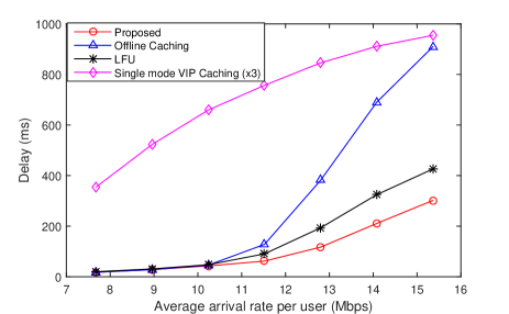
Figure 5: Delay versus per user average arrival rate with cache size $L_{C}=80$ data objects and skewness $\varsigma=0.5$.

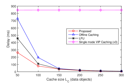
Figure 6: Delay versus cache size $L_{C}$ with per user average arrival rate $\lambda=13.25$ Mbps and skewness $\varsigma=0.5$.

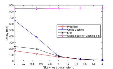
Figure 7: Delay versus skewness $\varsigma$ with per user average arrival rate $\lambda=13.25$ Mbps and cache size $L_{C}=80$ data objects.

Note that when the cache size $L_{C}$ or skewness $\varsigma$ is sufficiently large, the “cache hit” probability is high for any caching scheme, and thus the performance gap between different caching schemes will vanish, except for the single mode VIP caching scheme, which still has a large performance gap w.r.t. the proposed scheme because it cannot enjoy the cache-enabled opportunistic CoMP gain. However, the proposed scheme has significant gain over all the baseline schemes for practical scenarios when the cache size is limited compared to the total content size and the popularity does not concentrate on a few data objects. The fact that the proposed scheme achieves a better performance than the LFU demonstrates the effectiveness of the proposed mixed-timescale resource control algorithm based on the dual-mode VIP and Lyapunov optimization framework. The LFU can achieve a better performance than the offline caching scheme because it is an online caching scheme which can better adapts the cached content according to the microscopic spatial and temporary popularity variations. Finally, the single mode VIP caching scheme is worse than the other schemes because it cannot exploit the cache-enabled opportunistic CoMP to enhance the capacity of RAN.

VIII Conclusion

We propose a mixed-timescale online PHY caching and content delivery scheme for wireless NDNs with a dual-mode PHY. The cache content placement is performed once per frame ($T$ time slots) to avoid excessive cache content placement cost. For a given cache state at each frame, the PHY mode selection and rate allocation is performed once per time slot to fully exploit the cached content at the BS. To facilitate efficient resource control design, we introduce a dual-mode VIP framework, which transforms the original network into a virtual network, and formulate the resource control design in the virtual network. We establish the throughput optimality of the proposed solution. Moreover, we obtain a closed-form expression for the maximum sum DoF in the stability region under the Zipf popularity distribution. Simulations show that the proposed solution outperforms the existing offline PHY caching solution [6, 7] and online caching solutions [9].

-A Proof of Theorem 2

For a given $\boldsymbol{\lambda}\in\textrm{int}\Lambda_{v}$, the minimum cost $\overline{\Gamma}_{v}^{*}\left(\boldsymbol{\lambda}\right)$ for VIP stability is given by the solution of the problem in Theorem 3, minimized over the class of all stationary randomized policies defined in Section -C. If $\boldsymbol{\lambda}\in\textrm{int}\Lambda_{v}$, there exists a positive value $\epsilon$ such that $\boldsymbol{\lambda}+\boldsymbol{\epsilon}\in\textrm{int}\Lambda_{v}$. It follows that there exists a stationary random resource control policy $\left\{p_{n}^{k}(i),M\left(t\right),\mu_{j}^{Ak}(t),\mu_{j}^{Bk}(t),\mu_{ng}^{k}(t)\right\}$ in the virtual network such that the corresponding conditional flow balance constraint is satisfied:

$$\lambda_{j}^{k}+\epsilon \leq\overline{\mu}_{j|\boldsymbol{s}}^{Ak}+\overline{\mu}_{j|\boldsymbol{s}}^{Bk},$$

$$\sum_{j\in\mathcal{U}}\overline{\mu}_{j|\boldsymbol{s}}^{Ak}+\overline{\mu}_{j_{n}|\boldsymbol{s}}^{Bk} \leq\overline{\mu}_{ng|\boldsymbol{s}}^{k}+r_{n}s_{n}^{k}.$$ (44)

By modifying the rate allocation policy to $\mu_{j}^{Ak}(t)=\mu_{j}^{Ak}(t)-\frac{0.5\epsilon}{N+1}$ and $\mu_{j}^{Bk}(t)=\mu_{j}^{Bk}(t)-\frac{0.5\epsilon}{N+1}$, the resulting control policy satisfies the following conditional flow balance constraint:

$$\lambda_{j}^{k}+\frac{N\epsilon}{N+1} \leq\overline{\mu}_{j|\boldsymbol{s}}^{Ak}+\overline{\mu}_{j|\boldsymbol{s}}^{Bk},$$

$$\sum_{j\in\mathcal{U}}\overline{\mu}_{j|\boldsymbol{s}}^{Ak}+\overline{\mu}_{j_{n}|\boldsymbol{s}}^{Bk}+\frac{\epsilon}{2} \leq\overline{\mu}_{ng|\boldsymbol{s}}^{k}+r_{n}s_{n}^{k},$$ (45)

and we define $\overline{\Gamma}^{*}\left(\epsilon\right)$ as the minimum average cost consumed by any such stationary policy.

In the following, we construct a random control policy $\left\{p_{n}^{k}(i),m_{j}^{k}\left(t\right),c_{ng}(t),M_{a}\left(t\right),\boldsymbol{c}^{A}\left(t\right),\boldsymbol{c}^{B}\left(t\right)\right\}$ in the actual network such that the following conditional flow balance constraint is satisfied when the arrival rate tuple is $\boldsymbol{\lambda}$:

$$\overline{b}_{n|\boldsymbol{s}}+\frac{K\epsilon}{2} \leq\overline{c}_{ng|\boldsymbol{s}},\overline{b}_{nj_{n}|\boldsymbol{s}}^{B}+\frac{KN\epsilon}{2\left(N+1\right)}\leq\overline{c}_{j_{n}|\boldsymbol{s}}^{B},$$

$$\overline{b}_{nj|\boldsymbol{s}}^{A}+\frac{KN\epsilon}{2\left(N+1\right)}\leq\overline{c}_{j|\boldsymbol{s}}^{A}.$$ (46)

Specifically, the cache placement control policy $\left\{p_{n}^{k}(i)\right\}$ in the actual network is the same as that in the virtual network. For a given cache state $\boldsymbol{s}$, the forwarding mode at time slot $t$ in the actual plane is randomly chosen with $\Pr\left[m_{j}^{k}\left(t\right)=1\right]=\min\left(\left(\overline{\mu}_{j|\boldsymbol{s}}^{Ak}-\frac{N\epsilon}{2\left(N+1\right)}\right)/\lambda_{j}^{k},1\right)$. For the other control actions in the actual plane, we let $c_{ng}(t)=\sum_{k\in\mathcal{K}}\mu_{ng}^{k}(t)$, $M_{a}\left(t\right)=M\left(t\right)$, $\boldsymbol{c}^{A}\left(t\right)=\boldsymbol{\mu}^{A}\left(t\right)$ and $\boldsymbol{c}^{B}\left(t\right)=\boldsymbol{\mu}^{B}\left(t\right)$. Then, it can be verified that (46) is satisfied and the above control policy achieves the same average cost $\overline{\Gamma}^{*}\left(\epsilon\right)$ as that in the virtual network. (46) implies that the average departure rate of each DP queue is strictly larger than the average arrival rate, and hence the network is stable [11]. Therefore, we have proved that $\Lambda_{v}\subseteq\Lambda_{c}$. Moreover, following a similar argument to Footnote 3 in [11], it can be shown that $\overline{\Gamma}^{*}\left(\epsilon\right)\rightarrow\overline{\Gamma}_{v}^{*}\left(\boldsymbol{\lambda}\right)$ as $\epsilon\rightarrow 0$, so that stability in the actual network can be attained with an average cost that is arbitrarily close to $\overline{\Gamma}_{v}^{*}\left(\boldsymbol{\lambda}\right)$.

Similarly, it can be shown that for any $\boldsymbol{\lambda}\in\textrm{int}\Lambda_{c}$, the VIP stability in the virtual network can be attained with average cost that is arbitrarily close to $\overline{\Gamma}_{c}^{*}\left(\boldsymbol{\lambda}\right)$. This implies that $\Lambda_{c}\subseteq\Lambda_{v}$. Therefore, we have $\Lambda_{c}=\Lambda_{v}$ and $\overline{\Gamma}_{c}^{*}\left(\boldsymbol{\lambda}\right)=\overline{\Gamma}_{v}^{*}\left(\boldsymbol{\lambda}\right)$ for any arrival rate tuple $\boldsymbol{\lambda}\in\textrm{int}\Lambda_{v}$.

-B Proof of Theorem 3

Let $\Omega_{R}^{*}$ denote the optimal random policy (the optimal solution of (52)) in Lemma 3. Let $\Delta_{T}^{\text{R}}(i)$ denote the T-step drift-plus-penalty under $\Omega_{R}^{*}$.We first obtain an upper bound of $\Delta_{T}^{\text{R}}(i)$.

Lemma 1.

$\Delta_{T}^{\text{R}}(i)\leq\widetilde{\Delta}_{T}^{\text{R}}(i)=T^{2}B_{0}-T\epsilon\sum_{j\in N,k\in\mathcal{K}}V_{j}^{k}(t_{0})+TW\overline{\Gamma}_{v}^{*}\left(\boldsymbol{\lambda}\right)$, where $B_{0}$ is a constant depending on $\left\{\mu_{j,\text{max }}^{out},\mu_{n,\text{max }}^{out},\mu_{n,\text{max }}^{in}\right\}$ and $A_{\text{max}}$.

Proof:

Following a similar analysis to the proof of Theorem 3 in [15], it can be shown that

$$\Delta_{T}^{\text{R}}(i)\leq\widetilde{\Delta}_{T}^{\text{R}}(i)=T^{2}B_{0}+\Delta_{T1}^{\text{R}}(i)+\Delta_{T2}^{\text{R}}(i)+TW\overline{\Gamma}_{v}^{*}\left(\boldsymbol{\lambda}\right),$$

$$\widetilde{\Delta}_{T1}^{\text{R}}(i) =-2T\sum_{j\in\mathcal{U},k\in\mathcal{K}}V_{j}^{k}(t_{0}^{i})\mathbb{E}\bigg{[}\frac{1}{T}\sum_{\tau=t_{0}}^{t_{0}+T-1}\bigg{(}M^{*}\left(t\right)\sum_{j\in\mathcal{U}}\mu_{j}^{Ak*}(t)$$

$$+\overline{M}^{*}\left(t\right)\sum_{j\in\mathcal{U}}\mu_{j}^{Bk*}(t)\bigg{)}-\lambda_{n}^{k}|\boldsymbol{s}(i-1)\bigg{]},$$

$$\widetilde{\Delta}_{T2}^{\text{R}}(i) =-2T\sum_{j\in\mathcal{B},k\in\mathcal{K}}V_{j}^{k}(t_{0})\mathbb{E}\bigg{[}-\frac{1}{T}\sum_{\tau=t_{0}}^{t_{0}+T-1}\bigg{(}M^{*}\left(\tau\right)\sum_{j\in\mathcal{U}}\mu_{j}^{Ak*}(\tau)+\overline{M}^{*}\left(\tau\right)\sum_{j\in\mathcal{U}}\mu_{j}^{Bk*}(\tau)\bigg{)}$$

$$+\frac{1}{T}\sum_{\tau=t_{0}}^{t_{0}+T-1}\mu_{jg}^{k}(\tau)^{*}+r_{n}\left[s_{n}^{k}(t_{0}^{i}-1)+p_{n}^{k}(t_{0})^{*}\right]|\boldsymbol{s}(i-1)\bigg{]},$$

where the control actions with superscript ^∗ are given by the optimal random policy $\Omega_{R}^{*}$. Since for any given $\boldsymbol{s}(i)$, $\Omega_{R}^{*}$ satisfies the conditional flow balance (35), we have $\widetilde{\Delta}_{T1}^{\text{R}}(i)\leq-2T\sum_{j\in\mathcal{U},k\in\mathcal{K}}V_{j}^{k}(t_{0}^{i})\epsilon$ and $\widetilde{\Delta}_{T2}^{\text{R}}(i)\leq-2T\sum_{j\in\mathcal{B},k\in\mathcal{K}}V_{j}^{k}(t_{0}^{i})\epsilon$, from which Lemma 1 follows. ∎

To obtain an upper bound of the drift for the proposed solution, we need to consider a FRAME policy which serves as a bridge to connect the proposed solution and the optimal random policy $\Omega_{R}^{*}$. In the FRAME policy, the cache content placement is the same as the proposed solution, while the mode selection and rate allocation is the optimal solution of a modified version of the drift minimization problem in (23), with the current VIP length $\left\{V_{j}^{k}(t),V_{n}^{k}(t)\right\}$ replaced by the outdated VIP length $\left\{V_{j}^{k}(t_{0}^{i}),V_{n}^{k}(t_{0}^{i})\right\}$. Let $\widetilde{\Delta}_{T}^{\textrm{P}}(i)$ and $\widetilde{\Delta}_{T}^{\textrm{F}}(i)$ denote the upper bound of the T-step drift-plus-penalty defined in Theorem 1 under the proposed solution and the FRAME policy respectively. The following lemma states the relationship between the different policies.

Lemma 2.

$\widetilde{\Delta}_{T}^{\textrm{P}}(i)-\widetilde{\Delta}_{T}^{\textrm{F}}(i)\leq T^{2}B_{1}$, where $B_{1}$ is a constant depending on $\mu_{n,\text{max }}^{out}$, $\mu_{n,\text{max }}^{in}$ and $A_{\text{max}}$. Moreover, $\widetilde{\Delta}_{T}^{\text{F}}(i)\leq\widetilde{\Delta}_{T}^{\text{R}}(i)$.

Proof:

Similar to the proof of Lemma 5 in [15], the result $\widetilde{\Delta}_{T}^{\textrm{P}}(i)-\widetilde{\Delta}_{T}^{\textrm{F}}(i)\leq T^{2}B_{1}$ follows from the fact that the expected magnitude of change in a single VIP queue is at most $(\mu_{j,\text{max }}^{out}+A_{\text{max}}),\forall j\in\mathcal{U}$ and $(\mu_{n,\text{max }}^{out}+\mu_{n,\text{max }}^{in}+r_{n}),\forall n\in\mathcal{B}$, and the caching-related term in $\widetilde{\Delta}_{T}^{\textrm{P}}(i)$ and $\widetilde{\Delta}_{T}^{\textrm{F}}(i)$ is identical. The detailed proof is omitted for conciseness. On the other hand, the result $\widetilde{\Delta}_{T}^{\text{F}}(i)\leq\widetilde{\Delta}_{T}^{\text{R}}(i)$ follows from the fact that the FRAME policy minimizes $\widetilde{\Delta}_{T}\left(i\right)$. ∎

From Lemma 1 and 2, we conclude that

$$\Delta_{T}^{\textrm{P}}(i) \leq\widetilde{\Delta}_{T}^{\textrm{P}}(i)\leq\widetilde{\Delta}_{T}^{\text{F}}(i)+T^{2}B_{1}$$

$$\leq T^{2}B-T\epsilon\sum_{j\in N,k\in\mathcal{K}}V_{j}^{k}(t_{0})+TW\overline{\Gamma}_{v}^{*}\left(\boldsymbol{\lambda}\right),$$ (47)

where $B\triangleq B_{0}+B_{1}$. Finally, Theorem 3 can be proved from (47) by applying Theorem 4.2 of [12] and the same technique as in Theorem 3 of [15].

-C Proof of Theorem 4

Consider a stationary random policy $\Omega_{R}$ as follows. At the beginning of the $i$-th frame, $\left\{p_{n}^{k}(i)\right\}$ is randomly chosen from the set of all feasible cache placement control actions $\mathcal{A}_{p}^{\boldsymbol{s}^{{}^{\prime}}}$ (i.e., satisfying the cache size constraint (9)) with probability $\boldsymbol{\alpha}_{p}^{\boldsymbol{s}^{{}^{\prime}}}=\left[\alpha_{p1}^{\boldsymbol{s}^{{}^{\prime}}},...,\alpha_{p\left|\mathcal{A}_{p}^{\boldsymbol{s}^{{}^{\prime}}}\right|}^{\boldsymbol{s}^{{}^{\prime}}}\right]$, where $\boldsymbol{s}^{{}^{\prime}}=\boldsymbol{s}\left(i-1\right)$. Here, we use the superscript $\boldsymbol{s}^{{}^{\prime}}$ to indicate that $\mathcal{A}_{p}^{\boldsymbol{s}^{{}^{\prime}}}$ and $\boldsymbol{\alpha}_{p}^{\boldsymbol{s}^{{}^{\prime}}}$ depend on $\boldsymbol{s}^{{}^{\prime}}$. At each time slot $t$, $M\left(t\right)$ is randomly chosen with $\Pr\left[M\left(t\right)=0\right]=\alpha_{M}^{\left(\boldsymbol{s},\boldsymbol{H}\right)}$ and $\Pr\left[M\left(t\right)=1\right]=1-\alpha_{M}^{\left(\boldsymbol{s},\boldsymbol{H}\right)}$, where $\boldsymbol{s}=\boldsymbol{s}\left(i\right)$ and $\boldsymbol{H}=\boldsymbol{H}\left(t\right)$; $\mu_{j}^{Ak}\left(t\right)$ is randomly chosen from $N+1$ rate tuples $\left\{\mu_{ji}^{Ak\left(\boldsymbol{s},\boldsymbol{H}\right)},i=1,...,N+1\right\}$ satisfying

$$\left[\sum_{k\in\mathcal{K}}\mu_{ji}^{Ak\left(\boldsymbol{s},\boldsymbol{H}\right)}\right]_{j\in\mathcal{U}}\in C^{A}\left(\boldsymbol{H}\right),i=1,...,N+1,$$ (48)

with probability $\boldsymbol{\alpha}_{A}^{\left(\boldsymbol{s},\boldsymbol{H}\right)}=\left[\alpha_{A1}^{\left(\boldsymbol{s},\boldsymbol{H}\right)},...,\alpha_{A\left(N+1\right)}^{\left(\boldsymbol{s},\boldsymbol{H}\right)}\right]$; $\mu_{j}^{Bk}\left(t\right)$ is randomly chosen from $N+1$ rate tuples $\left\{\mu_{ji}^{Bk\left(\boldsymbol{s},\boldsymbol{H}\right)},i=1,...,N+1\right\}$ satisfying

$$\left[\sum_{k\in\mathcal{K}}\mu_{ji}^{Bk\left(\boldsymbol{s},\boldsymbol{H}\right)}\right]_{j\in\mathcal{U}}\in C^{B}\left(\boldsymbol{H}\right),i=1,...,N+1,$$ (49)

with probability $\boldsymbol{\alpha}_{B}^{\left(\boldsymbol{s},\boldsymbol{H}\right)}=\left[\alpha_{B1}^{\left(\boldsymbol{s},\boldsymbol{H}\right)},...,\alpha_{B\left(N+1\right)}^{\left(\boldsymbol{s},\boldsymbol{H}\right)}\right]$; and $\mu_{ng}^{k}(t)=\mu_{ng}^{k\left(\boldsymbol{s},\boldsymbol{H}\right)}$ satisfying

$$\sum_{k\in\mathcal{K}}\mu_{ng}^{k\left(\boldsymbol{s},\boldsymbol{H}\right)}\leq R_{d}.$$ (50)

Moreover, the above random policy $\Omega_{R}=\left\{\mathcal{A}_{p}^{\boldsymbol{s}^{{}^{\prime}}},\boldsymbol{\alpha}_{p}^{\boldsymbol{s}^{{}^{\prime}}},\alpha_{M}^{\left(\boldsymbol{s},\boldsymbol{H}\right)},\mu_{ji}^{Ak\left(\boldsymbol{s},\boldsymbol{H}\right)},\boldsymbol{\alpha}_{A}^{\left(\boldsymbol{s},\boldsymbol{H}\right)},\mu_{ji}^{Bk\left(\boldsymbol{s},\boldsymbol{H}\right)},\boldsymbol{\alpha}_{B}^{\left(\boldsymbol{s},\boldsymbol{H}\right)},\mu_{ng}^{k\left(\boldsymbol{s},\boldsymbol{H}\right)}\right\}$ is called a stationary random policy if the resulting Markov cache state process $\boldsymbol{s}\left(i\right)$ is stationary. Let $P_{\boldsymbol{s}^{{}^{\prime}},\boldsymbol{s}}^{\Omega_{R}}$ denote the transition probability of the controlled Markov Process $\boldsymbol{s}\left(i\right)$ from state $\boldsymbol{s}^{{}^{\prime}}$ to state $\boldsymbol{s}$, and $\pi_{\boldsymbol{s}}^{\Omega_{R}}$ denote the steady state probability of $\boldsymbol{s}\left(i\right)=\boldsymbol{s}$, under the stationary random policy $\Omega_{R}$. Then we have the following lemma.

Lemma 3 (VIP stability region).

The VIP stability region $\Lambda_{v}$ consists of all arrival rate tuples $\boldsymbol{\lambda}$ such that there exists a stationary random policy $\Omega_{R}$ satisfying (48), (49), (50) and

$$\lambda_{j}^{k}\leq\mathbb{E}_{\boldsymbol{H}}\bigg{[}\left(1-\alpha_{M}^{\left(\boldsymbol{s},\boldsymbol{H}\right)}\right)\sum_{i=1}^{N+1}\alpha_{Ai}^{\left(\boldsymbol{s},\boldsymbol{H}\right)}\mu_{ji}^{Ak\left(\boldsymbol{s},\boldsymbol{H}\right)}+\alpha_{M}^{\left(\boldsymbol{s},\boldsymbol{H}\right)}\sum_{i=1}^{N+1}\alpha_{Bi}^{\left(\boldsymbol{s},\boldsymbol{H}\right)}\mu_{ji}^{Bk\left(\boldsymbol{s},\boldsymbol{H}\right)}\bigg{]},$$

$$\mathbb{E}_{\boldsymbol{H}}\bigg{[}\left(1-\alpha_{M}^{\left(\boldsymbol{s},\boldsymbol{H}\right)}\right)\sum_{j\in\mathcal{U}}\sum_{i=1}^{N+1}\alpha_{Ai}^{\left(\boldsymbol{s},\boldsymbol{H}\right)}\mu_{ji}^{Ak\left(\boldsymbol{s},\boldsymbol{H}\right)}+\alpha_{M}^{\left(\boldsymbol{s},\boldsymbol{H}\right)}\sum_{i=1}^{N+1}\alpha_{Bi}^{\left(\boldsymbol{s},\boldsymbol{H}\right)}\mu_{j_{n}i}^{Bk\left(\boldsymbol{s},\boldsymbol{H}\right)}\bigg{]}\leq\mathbb{E}_{\boldsymbol{H}}\left[\mu_{ng}^{k\left(\boldsymbol{s},\boldsymbol{H}\right)}\right]+r_{n}s_{n}^{k},$$ (51)

$\forall j\in\mathcal{U},k\in\mathcal{K},n\in\mathcal{B}$ and $\forall\boldsymbol{s}\in\mathcal{S}$. Moreover, for any $\boldsymbol{\lambda}\in\textrm{int}\Lambda_{v}$, the minimum cache content placement cost required for stability $\overline{\Gamma}_{v}^{*}\left(\boldsymbol{\lambda}\right)$ is given by

$$\overline{\Gamma}_{v}^{*}\left(\boldsymbol{\lambda}\right)=\min_{\Omega_{R}} \sum_{\left(\boldsymbol{s}^{{}^{\prime}},\boldsymbol{s}\right)\in\mathcal{S}_{T}}\pi_{\boldsymbol{s}^{{}^{\prime}}}^{\Omega_{R}}P_{\boldsymbol{s}^{{}^{\prime}},\boldsymbol{s}}^{\Omega_{R}}\sum_{n\in\mathcal{B},k\in\mathcal{K}}\boldsymbol{1}_{\left\{s_{n}^{k}-s_{n}^{{}^{\prime}k}=1\right\}}$$ (52)

s.t. $$(\ref{eq:RdC1con}),\>(\ref{RdC0con}),\>(\ref{eq:Rdbkcon})\text{ and }(\ref{eq:RdCondflow})\text{ are satisfied}$$

$$\forall j\in\mathcal{U},k\in\mathcal{K},n\in\mathcal{B},\boldsymbol{s}\in\mathcal{S}.$$

Proof:

The proof involves showing that $\boldsymbol{\lambda}\in\Lambda_{v}$ is necessary for stability and that $\boldsymbol{\lambda}\in\textrm{int}\Lambda_{v}$ is sufficient for stability. First, we show $\boldsymbol{\lambda}\in\Lambda_{v}$ is necessary for stability. We take the arrival and departure at the base stations for example and the same technique can be applied to the virtual queues at the end users. By Lemma 1 of [15], network stability implies there exists a finite $Z$ such that $V_{n}^{k}(t)\leq Z$ for all $n\in\mathcal{B}$ and $k\in\mathcal{K}$ holds infinitely often. Given an arbitrarily small value $\epsilon>0$, there exists a slot $\widetilde{t}$ such that

$$V_{n}^{k}(\widetilde{t})\leq Z,\quad\frac{Z}{\widetilde{t}}\leq\epsilon.$$ (53)

Assuming $V_{n}^{k}(t_{0})=0$, we have

$$-V_{n}^{k}(t)\leq\sum_{\tau=t_{0}}^{t}F_{ng}^{k(\mathbf{s}(i),\boldsymbol{H}(\tau))}(\tau)+r_{n}\sum_{t=t_{0}}^{t}S_{n}^{k}(\tau)-\sum_{\tau=t_{0}}^{t}M(\tau)\sum_{j\in\mathcal{U}}F_{ji}^{Ak(\mathbf{s}(i),\boldsymbol{H}(\tau))}-\sum_{\tau=t_{0}}^{t}\overline{M}(\tau)\sum_{j\in\mathcal{U}}F_{j_{n}i}^{Bk(\mathbf{s}(i),\boldsymbol{H}(\tau))},$$ (54)

where $F_{ng}^{k(\mathbf{s}(i),\boldsymbol{H}(\tau))}(\tau)$ represents the actual virtual packet transmited through the backhual for content $k$ at time $\tau$. Thus, by 53 and 54, we have

$$0\leq\epsilon+\frac{1}{\widetilde{t}}\sum_{\tau=t_{0}}^{\widetilde{t}}F_{ng}^{k(\mathbf{s}(i),\boldsymbol{H}(\tau))}(\tau)+r_{n}\frac{1}{\widetilde{t}}\sum_{\tau=t_{0}}^{\widetilde{t}}S_{n}^{k}(\tau)-\frac{1}{\widetilde{t}}\sum_{\tau=t_{0}}^{\widetilde{t}}M(\tau)\sum_{j\in\mathcal{U}}F_{ji}^{Ak(\mathbf{s}(i),\boldsymbol{H}(\tau))}-\frac{1}{\widetilde{t}}\sum_{\tau=t_{0}}^{\widetilde{t}}\overline{M}(\tau)\sum_{j\in\mathcal{U}}F_{j_{n}i}^{Bk(\mathbf{s}(i),\boldsymbol{H}(\tau))}.$$ (55)

Note that the VIP stability region is defined under conditional flow balance. Given 55, it remains to prove that the constructed stationary random policy $\Omega_{R}$ satisfies the posed requirements. By letting $\epsilon\rightarrow 0$ or $\frac{1}{\widetilde{t}}\rightarrow\infty$, the total virutal packets drained by cache $r_{n}\frac{1}{\widetilde{t}}\sum_{\tau=t_{0}}^{\widetilde{t}}S_{n}^{k}(\tau)$ converges to its steady state distribution $r_{n}s_{n}^{k}$. For the rate allocatation terms such as $\frac{1}{\widetilde{t}}\sum_{\tau=t_{0}}^{\widetilde{t}}M(\tau)\sum_{j\in\mathcal{U}}F_{ji}^{Ak(\mathbf{s}(i),\boldsymbol{H}(\tau))}$, since the evolution of the cache state and channel state is independent of the rate allocation decision, and for each given $\mathbf{s}$, $\frac{1}{\widetilde{t}}\sum_{\tau=t_{0}}^{\widetilde{t}}M(\tau)\sum_{j\in\mathcal{U}}F_{ji}^{Ak(\mathbf{s},\boldsymbol{H}(\tau))}\rightarrow\mathbb{E}_{\boldsymbol{H}}\bigg{[}\left(1-\alpha_{M}^{\left(\boldsymbol{s},\boldsymbol{H}\right)}\right)\sum_{j\in\mathcal{U}}\sum_{i=1}^{N+1}\alpha_{Ai}^{\left(\boldsymbol{s},\boldsymbol{H}\right)}\mu_{ji}^{Ak\left(\boldsymbol{s},\boldsymbol{H}\right)}\bigg{]}$. By applying the steady state distribution of $\mathbf{s}$, 51 follows. Next, we show $\boldsymbol{\lambda}\in\textrm{int}\Lambda_{v}$ is sufficient for stability. By apply the condition 51, we have for each virtual queue, the arrival rate is less than the service rate, so the network is stable. ∎

Finally, Theorem 4 follows from Lemma 3 and the definition of $\mathcal{D}_{ve}$.

-D Proof of Theorem 5

It follows from the symmetry property of the problem that $\mu_{j}^{Ak}=\mu^{Ak},\forall j$ and $\mu_{j}^{Bk}=\mu^{Bk},\forall j$ at the optimal solution of (40). As a result, when $r_{n}\geq ND^{A}$, Problem (40) is equivalent to the following problem:

$$\max_{d,\alpha,\mu^{Ak},\mu^{Bk}}Kd,\text{ s.t. }d\rho_{k}=\left(1-\alpha\right)\mu^{Ak}+\alpha\mu^{Bk},\forall k$$

$$N\left(1-\alpha\right)\sum_{k=L_{c}+1}^{K}\mu^{Ak}+\alpha\sum_{k=L_{c}+1}^{K}\mu^{Bk}\leq R_{d},$$

$$\sum_{k\in\mathcal{K}}\mu^{Ak}\leq D_{A},\>\sum_{k\in\mathcal{K}}\mu^{Bk}\leq D_{B}.$$

By finding the optimal solution of the above problem, we can obtain the maximum sum DoF as in Theorem 5.

References

- [1] J. Li, W. Chen, M. Xiao, F. Shu, and X. Liu, “Efficient video pricing and caching in heterogeneous networks,” IEEE Transactions on Vehicular Technology, vol. 65, no. 10, pp. 8744–8751, Oct 2016.
- [2] J. Li, J. Sun, Y. Qian, F. Shu, M. Xiao, and W. Xiang, “A commercial video-caching system for small-cell cellular networks using game theory,” IEEE Access, vol. 4, pp. 7519–7531, 2016.
- [3] N. Golrezaei, K. Shanmugam, A. G. Dimakis, A. F. Molisch, and G. Caire, “Femtocaching: Wireless video content delivery through distributed caching helpers,” in Proc. IEEE INFOCOM. IEEE, 2012, pp. 1107–1115.
- [4] J. Dai, F. Liu, B. Li, B. Li, and J. Liu, “Collaborative caching in wireless video streaming through resource auctions,” IEEE Journal on Selected Areas in Communications, vol. 30, no. 2, pp. 458–466, 2012.
- [5] M. Ji, G. Caire, and A. F. Molisch, “Fundamental limits of distributed caching in D2D wireless networks,” in 2013 IEEE Information Theory Workshop (ITW), pp. 1–5.
- [6] A. Liu and V. K. Lau, “Mixed-timescale precoding and cache control in cached MIMO interference network,” IEEE Trans. Signal Process., vol. 61, no. 24, pp. 6320–6332, 2013.
- [7] ——, “Cache-enabled opportunistic cooperative MIMO for video streaming in wireless systems,” IEEE Trans. Signal Process., vol. 62, no. 2, pp. 390–402, 2014.
- [8] N. Abedini and S. Shakkottai, “Content caching and scheduling in wireless networks with elastic and inelastic traffic,” IEEE/ACM Transactions on Networking, vol. 22, no. 3, pp. 864–874, 2014.
- [9] E. Yeh, T. Ho, Y. Cui, M. Burd, R. Liu, and D. Leong, “VIP: A framework for joint dynamic forwarding and caching in named data networks,” in Proceedings of the 1st International Conference on Information-centric Networking, 2014, pp. 117–126.
- [10] M. M. Amble, P. Parag, S. Shakkottai, and L. Ying, “Content-aware caching and traffic management in content distribution networks,” in 2011 Proceedings IEEE INFOCOM, April 2011, pp. 2858–2866.
- [11] M. J. Neely, “Energy optimal control for time-varying wireless networks,” IEEE Trans. Inf. Theory, vol. 52, no. 7, pp. 2915–2934, 2006.
- [12] ——, “Stochastic network optimization with application to communication and queueing systems,” Synthesis Lectures on Communication Networks, vol. 3, no. 1, pp. 1–211, 2010.
- [13] A. Liu, V. Lau, W. Ding, and E. Yeh, “Mixed timescale online PHY caching and content delivery for content-centric wireless networks,” in GLOBECOM 2017 - 2017 IEEE Global Communications Conference, Dec 2017, pp. 1–6.
- [14] A. Liu and V. Lau, “Mixed-timescale precoding and cache control in cached MIMO interference network,” IEEE Trans. Signal Processing, vol. 61, no. 24, pp. 6320–6332, Dec 2013.
- [15] M. J. Neely, E. Modiano, and C. E. Rohrs, “Dynamic power allocation and routing for time-varying wireless networks,” IEEE Journal on Selected Areas in Communications, vol. 23, no. 1, pp. 89–103, 2005.
- [16] Q. Shi, M. Razaviyayn, Z.-Q. Luo, and C. He, “An iteratively weighted MMSE approach to distributed sum-utility maximization for a MIMO interfering broadcast channel,” IEEE Trans. Signal Processing, vol. 59, no. 9, pp. 4331 –4340, Sept. 2011.
- [17] R. Tandon, S. Mohajer, H. V. Poor, and S. Shamai, “Degrees of freedom region of the MIMO interference channel with output feedback and delayed CSIT,” IEEE Transactions on Information Theory, vol. 59, no. 3, pp. 1444–1457, March 2013.
- [18] T. Yamakami, “A Zipf-Like distribution of popularity and hits in the mobile web pages with short life time,” in Proc. Parallel Distrib. Comput., Appl. Technol., Taipei, Taiwan, Dec 2006, pp. 240–243.
- [19] Technical Specification Group Radio Access Network; Further Advancements for E-UTRA Physical Layer Aspects, 3GPP TR 36.814. [Online]. Available: http://www.3gpp.org