Neutron star structure in Hořava-Lifshitz gravity

Abstract

We present interesting aspects of neutron stars (NSs) from the standpoint of a modified theory of gravity called Hořava-Lifshitz (HL) gravity. A deviation from general relativity (GR) in HL gravity can change typical features of the NS structure. In this study, we investigate the NS structure by deriving the Tolman-Oppenheimer-Volkoff equation in HL gravity. We find that a NS in HL gravity with a larger radius and heavier mass than a NS in GR remains stable without collapsing into a black hole.

I Introduction

General relativity (GR) has been a successful theory of gravity for explaining the motion of planets and stars at the macroscopic scale up to now, because it is strongly valid under the weak gravitational field approximation. However, the theory is believed to be theoretically incomplete in terms of a unified theory with a quantum nature, for example, in describing the physics at strong gravitational fields near compact astrophysical objects such as black holes or neutron stars, mysterious darkness such as dark energy/matter, the origin of the Universe such as inflationary blowup, and the hierarchical phase transition at the very early stage of the Universe (see  Refs. Freese (2017); Silk (2013); Tsujikawa (2013); Guth (1981); Olive (1990); Brandenberger (2000); Boyanovsky et al. (2006) and the references therein). Although there have been many attempts to address these problems by introducing new particles and/or alternative theories of gravitation, a breakthrough is still required from the theoretical as well as experimental/observational point of view.

One of the discrepancies between gauge theories and GR is that the latter is not renormalizable due to ultraviolet (UV) divergence. The UV divergence appears in extreme circumstances and/or at high energies, where the quantum effect has to be taken into account, for example, at the early stage of the Universe or in the vicinity of a black hole. A renormalizable gravity theory is naturally supposed to have improved properties at the UV scale. One of the theories embodying such a philosophy has been proposed by Hořava Hořava ; Hořava (2009a, b) with the aim of formulating uv UV-complete theory by sacrificing local Lorentz symmetry, which is called Hořava-Lifshitz (HL) gravity. HL gravity approximates to GR at the infrared (IR) scale, whereas it becomes a different type of gravity at the UV scale by the introduction of anisotropic scaling between time and space. This anisotropic scaling is key to renormalizability in HL gravity although it breaks the local Lorentz symmetry. Many intensive studies in diverse fields of applications have been conducted in search of a possible candidate for quantum gravity (for recent progress reports, see Refs. Blas (2018); Wang (2017); Mukohyama (2010) and the references therein).

Further, the deformed HL gravity has been introduced to obtain asymptotically flat solutions by introducing a parameter $\omega$ in addition to the parameters in the original HL gravity Hořava (2009a); Park (2009). A static spherically symmetric and asymptotically flat solution has been found by Kehagias and Sfetsos (KS) Kehagias and Sfetsos (2009) that approaches the Schwarzschild black hole (SBH) at the IR limit. Among several parameters in the deformed HL gravity, $\omega$ is the only remaining free parameter appearing in the KS solution. The KS solution in the deformed HL gravity has been constrained by several observations in Refs. Liu et al. (2011); Horváth et al. (2011); Iorio and Ruggiero (2011). By introducing a dimensionless form $\tilde{\omega}=\omega(G_{N}c^{-2}M)^{2}$, the parameter is bounded from below, $\tilde{\omega}_{\mathrm{min}}\sim 10^{-17}$, $10^{-16}$, and $10^{-15}$, from light deflections by Jupiter, Earth, and the Sun, respectively Liu et al. (2011). $\tilde{\omega}_{\mathrm{min}}\sim 10^{-16}$ also originates from the weak lensing by galaxies of mass $\sim 10^{10}M_{\odot}$ Horváth et al. (2011). In addition, $\tilde{\omega}_{\mathrm{min}}\sim 10^{-10}$ is derived from the orbital motion of the S2 star Schödel et al. (2009) and the range residual of Mercury Iorio and Ruggiero (2011). These lower bounds are converted to $\omega_{\text{min}}\sim 10^{-48}-10^{-16}\ \text{cm}^{-2}$.

Here, one might ask how extreme circumstances can affect the structural equilibrium between HL gravity and isotropic matter. Tolman Tolman (1939) and Oppenheimer and Volkoff Oppenheimer and Volkoff (1939) (TOV) formulated the so-called TOV equation in GR to describe the equilibrium state of compact stars such as white dwarfs and NSs in a spherically symmetric and static configuration. By solving the Tolman-Oppenheimer-Volkoff (TOV) equation, we can obtain the mass-radius relation and, consequently, can estimate the maximum mass of a compact star and its radius. In particular, for a NS, the maximum mass and radius are sensitive to the stiffness of the selected equation-of-state (EOS) model. Hence, by investigating the TOV equation with the realistic EOS parameters, we can precisely understand the UV aspect of a NS in HL gravity in comparison with the case in GR. There have been many studies with diverse approaches to the stellar structure in HL gravity, for example, the stellar magnetic field configuration and the solution of Maxwell’s equations in HL gravity as well as in the modified $f(R)$ gravity Hakimov et al. (2013), black holes and stars with the projectability condition Greenwald et al. (2010), and gravitational collapse in HL gravity Greenwald et al. (2013). Other attempts at spontaneous scalarization in scalar-tensor gravity for compact stars have been studied in Refs. Salgado et al. (1998); Andreou et al. (2019); Rosca-Mead et al. (2020). Various aspects of a NS in different modified gravities were intensively studied in Refs. Astashenok et al. (2013, 2014, 2015a, 2015b); Kim (2014); Harko et al. (2013); Prasetyo et al. (2018); Barausse et al. (2011).

In this study, we investigate the structure of a NS in HL gravity, in comparison with that in GR. We derive an explicit form of the TOV equations in HL gravity. By solving them with realistic EOS models, we can obtain the mass-radius relation of a NS, which estimates how HL gravity deviates from GR in terms of the mass and the radius of a NS. In Sec. II, the TOV equation of perfect fluids in HL gravity is derived for this purpose. We then solve the equation in Sec. III with the selected EOS models of Akmal-Pandharipande-Ravenhall (APR4) Akmal et al. (1998), Müther-Prakash-Ainsworth (MPA1) Müther et al. (1987), Müller-Serot (MS1) Müller and Serot (1996), and Wiringa-Fiks-Fabrocini (WFF1) Wiringa et al. (1988) because, from the TOV calculation in GR, these models have shown results that are consistent with the observed maximum mass, $\sim$$2M_{\odot}$ of NSs Demorest et al. (2010); Linares et al. (2018). For the numerical computation of the TOV equation, we adopt the fifth-order Runge-Kutta solver Dormand and Prince (1980); Shampine (1986). The mass-radius relation in HL gravity is compared with that in GR, which shows that both the mass and the radius of the heaviest NS in HL gravity are larger than those in GR. It is shown that the distance-dependent profile of the pressure decreases more gradually, and the surface condition where the pressure becomes zero is satisfied at farther radii due to the relatively weaker gravitational attraction of HL gravity than that of GR. We address the detailed investigation into the mass-radius relation in HL gravity as well as the parametric limit of the HL parameter $\omega$ based on the result. Finally, we discuss our results in terms of observational validation in Sec. IV.

II TOV equation in HL gravity

The action of HL gravity is formulated by an anisotropic scaling between time and space, $t\rightarrow b^{z}t$ and $x^{i}\rightarrow bx^{i}$ and the form of $z=3$:

$$I_{\text{\acs{hl}}} = \int dtd^{3}x\sqrt{g}N\left[\frac{2}{\kappa^{2}}\left({\mathcal{K}}_{ij}{\mathcal{K}}^{ij}-\lambda{\mathcal{K}}^{2}\right)\right.$$ (1)

$$-\left.\frac{\kappa^{2}}{2\zeta^{4}}\left({\mathcal{C}}_{ij}-\frac{\mu\zeta^{2}}{2}{\mathcal{R}}_{ij}\right)\left({\mathcal{C}}^{ij}-\frac{\mu\zeta^{2}}{2}{\mathcal{R}}^{ij}\right)\right.$$

$$+\!\left.\!\frac{\kappa^{2}\mu^{2}(4\lambda\!-\!1)}{32(3\lambda\!-\!1)}\!\!\left(\!{\mathcal{R}}^{2}\!+\!\frac{4(\omega\!-\!\Lambda_{W})}{4\lambda\!-\!1}{\mathcal{R}}\!+\!\frac{12\Lambda_{W}^{2}}{4\lambda\!-\!1}\!\right)\!\right]$$

with the softly broken detailed balance condition, which is sometimes called the deformed HL gravity in the literature. Note that ${\mathcal{K}}_{ij}\equiv\frac{1}{2N}[\dot{g}_{ij}-\nabla_{i}N_{j}-\nabla_{j}N_{i}]$ is an extrinsic curvature, where $N$ is a lapse function, $N^{i}$ is a shift vector, $g_{ij}$ is a three-dimensional spatial metric, and $\dot{g}_{ij}$ denotes $\partial{}g_{ij}/\partial{}t$. ${\mathcal{C}}^{ij}\equiv\varepsilon^{ik\ell}\nabla_{k}({\mathcal{R}}_{\ell}^{j}-\delta_{\ell}^{j}{\mathcal{R}}/4)$ is a Cotton-York tensor, where ${\mathcal{R}}_{ij}$ and ${\mathcal{R}}$ are a three-dimensional spatial Ricci tensor and a Ricci scalar, respectively. $\kappa^{2}$ is a coupling related to the Newton constant $G_{N}$, and $\lambda$ is an additional dimensionless coupling constant. Here, $\omega$ is essential for an asymptotically flat solution, though it violates the detailed balance condition. The coupling constants $\mu$, $\Lambda_{W}$, and $\zeta$ stem from the three-dimensional Euclidean topologically massive gravity action Deser et al. (1982a, b). When $\lambda=1$, the Einstein-Hilbert action can be recovered in the IR limit by identifying the fundamental constants with $c=(\kappa^{2}/4)[\mu^{2}(\omega-\Lambda_{W})/(3\lambda-1)]^{1/2}$, $G_{N}=\kappa^{2}c^{2}/32\pi$, and $\Lambda=-(3/2)\Lambda_{W}^{2}/(\omega-\Lambda_{W})$, representing the speed of light, the gravitational constant, and the cosmological constant, respectively.

The total action under consideration is given by $I_{\text{tot}}=I_{\text{\acs{hl}}}+I_{\text{mat}}$, where $I_{\text{mat}}$ represents the matter action that will be specified by assuming a perfect fluid and choosing an EOS without an explicit form. In addition, we consider hereafter an asymptotically flat geometry, that is, $\Lambda=0$, for simplicity.

Now, if we consider a static, spherically symmetric metric ansatz,

$$ds^{2}=-e^{2\Phi(r)}c^{2}dt^{2}\!+\!\frac{dr^{2}}{1\!-\!f(r)}\!+\!r^{2}\!\left(d\theta^{2}\!+\!\sin^{2}\theta d\phi^{2}\right),$$ (2)

then the equations of motion in HL gravity with the stress-energy tensor of a perfect fluid, $T_{\mu\nu}=(\rho+p)u_{\mu}u_{\nu}+pg_{\mu\nu}$, are given by

$$\rho =\frac{c^{2}}{16\pi G_{N}r^{2}\omega}\left(2r\omega f+\frac{f^{2}}{r}\right)^{\prime},$$ (3a)

$$p =\frac{c^{4}}{16\pi G_{N}r^{4}\omega}\left[f\left(f-2r^{2}\omega\right)+4r\left(1-f\right)\left(f+r^{2}\omega\right)\Phi^{\prime}\right],$$ (3b)

$$p^{\prime} =-\left(\rho c^{2}+p\right)\Phi^{\prime},$$ (3c)

where $u_{\mu}=(1,0,0,0)$ is a four-vector field, $\rho$ and $p$ are the energy density and the pressure of a perfect fluid, respectively, and the prime denotes $d/dr$. Note that HL gravity has six parameters, as observed in Eq. (1): we have already fixed $\lambda$ and $\Lambda_{W}$ to 1 and 0, respectively, $\kappa$ and $\mu$ are hidden in the physical constants related to $c$ and $G_{N}$ in the IR region, and $\zeta$ does not contribute to this nonrotating configuration. Thus, $\omega$ is the only remaining free parameter of the theory under consideration.

To solve Eq. (3), we replace $f(r)$ by $m(r)$ through the relation $f=-r^{2}\omega+\sqrt{r\omega(r^{3}\omega+4G_{N}c^{-2}m)}$. Then, when $m(r)=M$, it approaches $f\xrightarrow{\omega\to\infty}2G_{N}c^{-2}M/r-2G_{N}^{2}c^{-4}\omega^{-1}M^{2}/r^{4}+\cdots$, where the first term is nothing but the Schwarzschild solution, and the following terms are HL corrections depending upon the $\omega$ parameter. Here, the mass parameter $M$ is identified as the quasilocal energy at infinity Myung (2010). For the KS solution, we see $e^{2\Phi(r)}=1-f(r)$, while Eq. (3c) governs the behavior of the $(tt)$-component of the metric, which is coupled to matter in the generic case. Note that the horizons of the KS black hole are located at $r_{\pm}=G_{N}c^{-2}\left(M\pm\sqrt{M^{2}-M_{c}^{2}}\right)$, where $M_{c}\equiv(2\omega G_{N}^{2}c^{-4})^{-1/2}$ is the critical mass of the horizons formed. With the Planck mass $m_{P}$ and length $l_{P}$, $M_{c}$ can be rewritten as $M_{c}=m_{P}/\sqrt{2\omega\ell_{P}^{2}}$, which reduces to $M_{c}=m_{P}/\sqrt{2}$ for $\omega=\ell_{P}^{-2}$ and becomes $M_{c}\approx M_{\odot}$ for $\omega\approx 2.293\times 10^{-11}\,\text{cm}^{-2}$. For a constant $\omega$, the black hole horizon exists with $M\geq M_{c}$. On the other hand, for a fixed $M$, one finds $\omega\geq\omega_{c}\equiv(2G_{N}^{2}c^{-4}M^{2})^{-1}$ to form a black hole. Hence, the horizon of a solar mass KS black hole exists only if $\omega\geq\omega_{c}\approx 2.293\times 10^{-11}\textrm{cm}^{-2}$. Requiring that a $4M_{\odot}$ black hole candidate, GRO J0422+32 Gelino and Harrison (2003), has the horizon, we have $\omega\gtrsim 1.433\times 10^{-12}\textrm{cm}^{-2}$. In this manner, we restrict the range of the parameter as $\omega\geq 2\times 10^{-12}\ \textrm{cm}^{-2}$.

Now, we can rewrite Eq. (3) as follows:

$$m^{\prime} =4\pi r^{2}\rho,$$ (4a)

$$p^{\prime} =\frac{(\rho c^{2}+p)r\omega\left[\left(1+\tilde{\rho}\right)-\sqrt{1+4\tilde{\rho}}-\tilde{p}\right]}{\sqrt{1+4\tilde{\rho}}\left[1+r^{2}\omega\left(1-\sqrt{1+4\tilde{\rho}}\right)\right]},$$ (4b)

where $\tilde{\rho}=G_{N}c^{-2}\omega^{-1}mr^{-3}$ and $\tilde{p}=4\pi G_{N}c^{-4}\omega^{-1}p$. Note that if we expand $p^{\prime}$ in terms of $1/\omega\rightarrow 0$ using the relation $\sqrt{1+\epsilon}\approx 1+\epsilon/2+\cdots$ for $\epsilon\ll 1$ and take the leading order, we obtain

$$p^{\prime}\approx-\frac{G_{N}m\rho}{r^{2}}\left(1+\frac{p}{\rho c^{2}}\right)\left(1+\frac{4\pi r^{3}p}{mc^{2}}\right)\left(1-\frac{2G_{N}m}{rc^{2}}\right)^{-1},$$ (5)

which reproduces the TOV equation in GR.

III NS Structure in HL gravity

For the study of the NS structure in GR, various EOS models have been taken into account. Among them, we, in particular, select four EOS models that result in the maximum mass, $M_{\mathrm{max}}$, of a NS becoming similar to or heavier than $2M_{\odot}$ from the conventional TOV calculation in GR, and the results agree with the recent observations of $\sim$$2M_{\odot}$ NS Demorest et al. (2010); Linares et al. (2018). The selected EOS models are APR4 Akmal et al. (1998), MPA1 Müther et al. (1987), MS1 Müller and Serot (1996), and WFF1 Wiringa et al. (1988): MPA1 and MS1 are, respectively, derived using the relativistic Brueckner-Hartree-Fock theory and the relativistic mean field theory. APR4 and WFF1 are derived with the variational method but with different nucleon potential models (see Ref. Akmal et al. (1998) for the difference in the used models). All of these models assume that the nuclear matter contains neutrons, protons, electrons, and muons. In addition, to imitate the crust structure near the surface of ns NS, we replace the low-density region of the considered EOS models with the Skyrme-Lyon model Douchin and Haensel (2001) as studied in Read et al. (2009).

To solve $m$ and $p$ in Eq. (4) simultaneously, we adopt the fifth-order Runge-Kutta method which controls the error with the fourth-order method Dormand and Prince (1980); Shampine (1986). For the computation, we first set $\rho\left(0\right)=\rho_{c}$, $p\left(0\right)=p_{c}$ at the center $r=0$, where we call $\rho_{c}$ and $p_{c}$ as the central density and pressure, respectively. We obtain $m\left(r\right)$ and $p\left(r\right)$ at each $r$ by taking $\left(\rho_{c},p_{c}\right)$ from each of the EOSs and solving Eq. (4) numerically. The radius $R$ is then determined by $R=r^{*}$ where $p(r=r^{*})=0$, and the mass is simultaneously determined by $M=m(R)$. Thus, by varying $\rho_{c}$, we produce the series of $\left(M,R\right)$ called the mass-radius relation, which describes the static profile of the spherically symmetric NS structure for a given EOS model. The exterior of the NS is naturally described by the KS vacuum solution $e^{2\Phi(r>R)}=1-f(r>R)=1+r^{2}\omega-\sqrt{r\omega(r^{3}\omega+4G_{N}c^{-2}M)}$, and an integration constant of the metric function $\Phi(r)$ is fixed by this boundary condition at $r=R$.

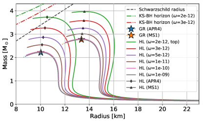
(a) APR4 and MS1 case

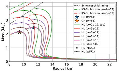
(b) MPA1 and WFF1 case

Figure 1: Plots of mass-radius relation in GR and HL with varying parameter $\omega$ for the selected EOS models.

In Fig. 1, we present the mass-radius relations in both HL gravity and GR, and the relation in GR is depicted with the star-marked maximum mass. The heaviest NS obtained in HL gravity is also marked by different symbols for each EOS model. We see that the mass and radius of a NS increase as $\omega$ becomes smaller. This result implies that HL gravity with a smaller $\omega$ deviates more than GR. We also place the horizon of a SBH and two horizons of a KS black hole (KSBH) with $\omega=2\times 10^{-12}\mathrm{cm}^{-12}$ and $\omega=3\times 10^{-12}\mathrm{cm}^{-12}$ at the top-left corner of Fig. 1; we observe that the radii of the maximum stable NSs in both HL gravity and GR under consideration are safely larger than the horizon radius of a black hole with the same mass.

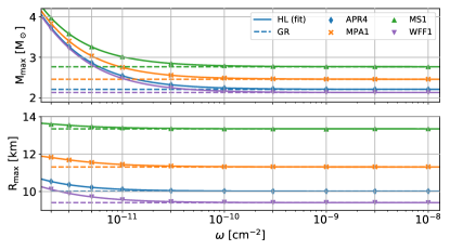
Figure 2: Plots of the effect of $\omega$ on the maximum mass and radius for the selected EOS models in GR and HL gravity.

We now focus on the $\omega$ dependency in the mass and radius. In Fig. 2, we present the $\omega$-dependent maximum mass (top panel) and radius (lower panel) obtained in HL gravity (solid lines) and GR (dashed lines) from each of the EOS models. We fit the data point with a curve via $M_{\text{max}}^{\text{\acs{hl}}}\approx M_{\text{max}}^{\text{\acs{gr}}}\left[1+\left(A_{1}\omega^{-1}+A_{2}\omega^{-2}\right)\right]$ and $R_{\text{max}}^{\text{\acs{hl}}}\approx R_{\text{max}}^{\text{\acs{gr}}}\left[1+\left(B_{1}\omega^{-1}+B_{2}\omega^{-2}\right)\right]$ to facilitate the $\omega$ dependency in the mass and radius in HL gravity and, consequently, to discuss the $\omega$-dependent difference between HL gravity and GR. The details of determined fitting coefficients are summarized in Table 1.

Table 1: Fitting coefficients for $M_{\text{max}}^{\text{\acs{hl}}}$ and $R_{\text{max}}^{\text{\acs{hl}}}$ with all considered EOS models.

EOS Models	Fitting Coefficients
	$A_{1}$	$A_{2}$	$B_{1}$	$B_{2}$
	$(\times 10^{-13})$	$(\times 10^{-26})$	$(\times 10^{-14})$	$(\times 10^{-27})$
APR4	15.3	-33.0	10.2	4.17
MPA1	12.0	-16.7	12.0	-60.7
MS1	8.92	-4.78	4.87	-21.2
WFF1	16.8	-42.3	17.4	-46.1

Here, we can see that HL gravity can reproduce GR when $\omega\gtrsim{\color[rgb]{0,0,0}1.68\times 10^{-9}}\textrm{cm}^{-2}$ or ${\color[rgb]{0,0,0}1.68\times 10^{-10}}\ \textrm{cm}^{-2}$ up to tolerances of $|\Delta M_{\text{max}}|\left(M_{\text{max}}^{\text{\acs{gr}}}\right)^{-1}\lesssim{\color[rgb]{0,0,0}10^{-3}}$ and $|\Delta R_{\text{max}}|\left(R_{\text{max}}^{\text{\acs{gr}}}\right)^{-1}\lesssim{\color[rgb]{0,0,0}10^{-2}}$, respectively, where $\Delta$ represents the difference between a quantity in HL gravity and that in GR. We observe that the profile of $M_{\mathrm{max}}$ and $R_{\mathrm{max}}$ with $\omega\gtrsim{\color[rgb]{0,0,0}1.68\times 10^{-9}}\ {\rm{cm^{-2}}}$ in HL gravity has the same behavior as that in GR for all the considered EOS models. We also observe that the smaller value of $\omega$ in HL gravity leads to a larger deviation from GR.

Next, we examine the $r$-dependent profiles at the interior of the NS. We discuss the $r$ dependency with the APR4 case only because it gives the closest maximum mass in GR to the upper limit of the NS mass Abbott et al. (2017) among the selected EOS models. In the upper panel of Fig. 3 (a), we plot mass profiles of the following NSs:

(i)	The heaviest NS in GR
(ii)	The heaviest NS in HL gravity
	($\omega=2\times 10^{-12}\ \textrm{cm}^{-2}$)
(iii)	The NS in HL gravity of the same mass $M^{\text{\acs{gr}}}_{\text{max}}$ as the NS in (i)
(iv)	The NS in HL gravity of the same central density $\rho_{c}$ as the NS in (i)

On the other hand, the gravitational accelerations inside the NSs corresponding to (i)–(iv) are plotted in the lower panel of Fig. 3 (a). The surface gravity of ns NS is given by $g_{\text{\acs{ns}}}$ Shapiro and Teukolsky (1983); Bejger and Haensel (2004). Similarly, the gravitational acceleration experienced by an observer on a fixed $r$ inside ns NS can be calculated as $a(r)=(1-f(r))^{1/2}\Phi^{\prime}(r)$, which naturally becomes $g_{\text{\acs{ns}}}$ at the surface $R$. We observe that HL gravity has a relatively weaker gravitational acceleration than that in GR near the central region of the NS. Even though the NS in (ii) is much heavier than the NS in (i), its gravity is weaker at $r\lesssim 6\ \mathrm{km}$. This observation explains why the heavier NS rather than the NS in (i) remains stable in HL gravity without collapsing into a black hole. The weaker gravity of HL is also observed from the curve of the same-mass NS in (iii) at the bottom panel of Fig. 3 (a). Note that the maximum accelerations inside the heaviest NSs are almost the same in both GR and HL gravity; however, the accelerations may be slightly different depending on the EOS models.

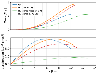
(a) mass and gravitational acceleration

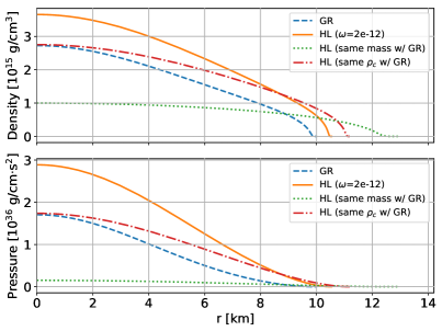
(b) density and pressure

Figure 3: $r$-dependent behaviors of (a) mass and acceleration and (b) density and pressure inside the NSs for the case of APR4 in GR and HL.

In addition, the profiles of the density and pressure inside NSs are also shown in the upper panel and lower panel, respectively, in Fig. 3 (b). Due to the weaker gravitational attraction inside the same-mass NS in (iii), the pressure and density increase slowly as $r$ goes to zero, and the central density becomes much smaller than that of the NS in (i), which is consistent with the larger radius of the NS in (iii). The central density of the NS in (iv) is the same as that of the NS in (i), and the density and pressure decrease slowly as $r$ increases and vanish at larger radii, with the result that the NS in (iv) becomes naturally heavier than the NS in (i). Note that the weaker gravitational attraction in HL gravity can be easily understood by computing the Kretschmann curvature scalar defined by $\mathscr{K}\equiv{\mathcal{R}}_{\alpha\beta\gamma\sigma}{\mathcal{R}}^{\alpha\beta\gamma\sigma}$. Indeed, the Kretschmann curvature scalar of the KSBH solution can be compared to that of the SBH solution with the same mass and radius. In GR, $\mathscr{K}_{\text{\acs{sbh}}}=48G_{N}^{2}c^{-4}M^{2}r^{-6}$, whereas $\mathscr{K}_{\text{\acs{ks}BH}}\xrightarrow{r\ll r_{c}}(81/4)G_{N}c^{-2}M\omega r^{-3}[1+O(r/r_{c})^{3/2}]$ and $\mathscr{K}_{\text{\acs{ks}BH}}\xrightarrow{r\gg r_{c}}\mathscr{K}_{\text{\acs{sbh}}}[1+O(r_{c}/r)^{3}]$ in HL gravity, where $r_{c}\equiv(4G_{N}c^{-2}M\omega^{-1})^{1/3}$ is a characteristic scale of the KSBH solution. The overall behavior of the Kretschmann curvature scalar for the KSBH solution in HL is slowly growing, unlike the SBH solution in GR, which implies that the gravitational force induced by the curvature scalar in HL gravity is weaker than that in GR in the limit of $r\rightarrow 0$. Then the mass obtained by integrating Eq. (4a) from $r=0$ to $r=R$ also becomes heavier, eventually. However, the results of $M_{\textrm{max}}\gtrsim 3M_{\odot}$ in HL gravity are placed not only beyond the upper limit of the theoretical estimation of the upper limit Bombaci (1996); Kalogera and Baym (1996) but far beyond the upper limit of the mass of a NS Demorest et al. (2010); Linares et al. (2018); Margalit and Metzger (2017); Shibata et al. (2017); Ruiz et al. (2018); Rezzolla et al. (2018).

IV Discussions

We have discussed the characteristics of HL gravity by examining the $\omega$ dependency of the physical observables, especially, mass and radius, of a NS. The considered range of $\omega\geq 2\times 10^{-12}\ \text{cm}^{-2}$ has been chosen based on the lower bounds determined by observations, $\omega_{\text{min}}\sim 10^{-16}\ \text{cm}^{-2}$, and the cosmic censorship for a $4\ M_{\odot}$ black hole candidate, GRO J0422+32, that reads $\omega\geq 1.433\times 10^{-12}\ \textrm{cm}^{-2}$.

The conventional measurement of the mass and radius of a NS is conducted by observations on a pulsar, rotating NS, consisting of a binary system. Depending upon the type of pulsar, different approaches have been implemented to measure or to constrain the mass and radius (for more details, see Ref. Özel and Freire (2016) and the references therein). In addition, from the recent detection of GW170817, radiated from a merger of binary NS systems, it is now possible to consider the gravitational wave (GW) as an additional approach to estimating the mass and radius of a NS Abbott et al. (2017, 2018). In addition, a possible problem of the exclusion of HL gravity was raised with the help of GW170817 by a comparison between the speeds of GW and the electromagnetic wave, the polarization of GWs and so on Creminelli and Vernizzi (2017); Ezquiaga and Zumalacárregui (2017); Yagi et al. (2014a, b). However, there are also unconstrained parameter regions that favor HL gravity even after the observation of GW170817 Barausse (2019), and the problem requires further studies. Hence, to discuss the viability of HL gravity with the physical observables of a NS, it is worthwhile to address some aspects of HL gravity more rigorously such as (i) whether it can pass the tests on post-Keplerian parameters Özel and Freire (2016), (ii) whether it is possible to derive GW waveforms with HL gravity to perform parameter estimation as done with GR, and (iii) how the tidal deformability of a NS in HL gravity differs from that in GR, and so on.

HL gravity is also open to the possibility of being verified through other compact objects such as black holes and white dwarfs. HL gravity was originally designed for recovering the usual asymptotic property of GR whereas it has a UV modification in the strong gravity region unlike GR. An observer in the IR region can always experience the asymptotic structure of the object rather than the UV structure. The feature of the UV structure is only reflected in the physical parameters such as mass, spin, and so on. Thus, one finds that the stellar mass black hole behaves consistently no matter how large/small its mass is once the black hole forms whereas the only differences are the deviation of physical parameters encoded by the UV structures of black holes. As shown in the KS solution, it clearly looks like a SBH at large distances of $r$ whereas it differs from the SBH as $r$ goes to the UV region. The extent of the difference between HL gravity and GR depends upon the parameter $\omega$. The relatively large $\omega$ leads to the small deviation from GR because we have the form of the KS solution: $f(r)=2k/r(1-k/\omega r^{3}+\cdots)$, where $k=G_{N}M/c^{2}$. Therefore, we may constrain the lower bound of $\omega$ further from the mass of the stellar mass black holes which can be estimated by the GW and/or x-ray observations.

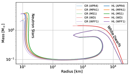
Figure 4: Plots of mass-radius relation in GR and HL with $\omega=2\times 10^{-12}\ \mathrm{cm}^{-2}$ for the EOS models for NSs under consideration (APR4, MS1, MPA1, and WFF1) and the relativistic EOS for white dwarf (WD).

Now, it is noteworthy that the EOS models for the NS structure do not show significant differences in the structure of a white dwarf. This is primarily because they are almost identical except for the physics at the nucleus size. Similarly, HL gravity deforms the behavior at UV scale and does not change the structure of a white dwarf significantly. The behaviors of white dwarfs as well as NSs in GR and HL gravity are depicted in Fig. 4. The relativistic EOS for white dwarfs is obtained by assuming that the dominant chemical components of white dwarfs are ⁴He, ¹²C, or ¹⁶O, that is, the ratio between the atomic mass number $A$ and the number of electrons $Z$ is given by $A/Z=2$ Sagert et al. (2006). The EOS models for NSs do not reflect the Chandrasekhar limit correctly, because they are obtained by considering physical situations beyond the degeneracy pressure of electrons such as neutronization. The mass-radius relation of white dwarfs in the beyond Horndeski class of gravity theories was investigated in Saltas et al. (2018).

In conclusion, it is shown that HL gravity reveals a deviant feature from GR in the short distance regime due to its relatively weaker gravitational force compared with that of GR. We observe that the deviation is sensitive to the choice of parameter $\omega$. In addition, the NS with the larger radius and the heavier mass is far beyond the upper limit of the current observational results obtained from GR or post-Keplerian. To validate HL gravity, theoretical investigations and future observations of GWs from compact binary mergers containing at least one NS will yield more constraints on the physical observables of a NS and, eventually, will determine the fate of HL gravity.