Collision fluctuations of lucky droplets with superdroplets

Abstract

It was previously shown that the superdroplet algorithm for modeling the collision-coalescence process can faithfully represent mean droplet growth in turbulent clouds. But an open question is how accurately the superdroplet algorithm accounts for fluctuations in the collisional aggregation process. Such fluctuations are particularly important in dilute suspensions. Even in the absence of turbulence, Poisson fluctuations of collision times in dilute suspensions may result in substantial variations in the growth process, resulting in a broad distribution of growth times to reach a certain droplet size. We quantify the accuracy of the superdroplet algorithm in describing the fluctuating growth history of a larger droplet that settles under the effect of gravity in a quiescent fluid and collides with a dilute suspension of smaller droplets that were initially randomly distributed in space (‘lucky droplet model’). We assess the effect of fluctuations upon the growth history of the lucky droplet and compute the distribution of cumulative collision times. The latter is shown to be sensitive enough to detect the subtle increase of fluctuations associated with collisions between multiple lucky droplets. The superdroplet algorithm incorporates fluctuations in two distinct ways: through the random spatial distribution of superdroplets and through the Monte Carlo collision algorithm involved. Using specifically designed numerical experiments, we show that both on their own give an accurate representation of fluctuations. We conclude that the superdroplet algorithm can faithfully represent fluctuations in the coagulation of droplets driven by gravity.

1 Introduction

Direct numerical simulations (DNS) have become an essential tool to investigate collisional growth of droplets in turbulence (Onishi et al., 2015; Saito and Gotoh, 2018). Here, DNS refers to the realistic modeling of all relevant processes, which involves not only the use of a realistic viscosity, but also a realistic modeling of collisions of droplet pairs in phase space. The most natural and physical way to analyze collisional growth is to track individual droplets and to record their collisions, one by one. However, DNS of the collision-coalescence process are very challenging, not only when a large number of droplets must be tracked, but also because the flow must be resolved over a large range of time and length scales.

Over the past few decades, an alternative way of modeling aerosols has gained popularity. Zannetti (1984) introduced the concept of “superparticles, i.e., simulation particles representing a cloud of physical particles having similar characteristics.” This concept was also used by Paoli et al. (2004) in the context of condensation problems. The application to coagulation problems was pioneered by Zsom and Dullemond (2008) and Shima et al. (2009), who also developed a computationally efficient algorithm. The idea is to combine physical cloud droplets into ‘superdroplets’. To gain efficiency, one tracks only superdroplet collisions and uses a Monte Carlo algorithm (Sokal, 1997) to account for collisions between physical droplets. This is referred to as “superdroplet algorithm.” It is used in both the meteorological literature (Shima et al., 2009; Sölch and Kärcher, 2010; Riechelmann et al., 2012; Arabas and Shima, 2013; Naumann and Seifert, 2015, 2016; Unterstrasser et al., 2017; Dziekan and Pawlowska, 2017; Li et al., 2017, 2018, 2019, 2020; Sato et al., 2017; Jaruga and Pawlowska, 2018; Brdar and Seifert, 2018; Sato et al., 2018; Seifert et al., 2019; Hoffmann et al., 2019; Dziekan et al., 2019; Grabowski et al., 2019; Shima et al., 2020; Grabowski, 2020; Unterstrasser et al., 2020), as well as in the astrophysical literature (Zsom and Dullemond, 2008; Ormel et al., 2009; Zsom et al., 2010; Johansen et al., 2012, 2015; Ros and Johansen, 2013; Drakowska et al., 2014; Kobayashi et al., 2019; Baehr and Klahr, 2019; Ros et al., 2019; Nesvornỳ et al., 2019; Yang and Zhu, 2020; Poon et al., 2020; Li and Mattsson, 2020, 2021). Compared with DNS, the superdroplet algorithm is distinctly more efficient. It has been shown to accurately model average properties of droplet growth in turbulent clouds. Li et al. (2018) demonstrated, for example, that the mean collision rate obtained using the superdroplet algorithm agrees with the mean turbulent collision rate (Saffman and Turner, 1956) when the droplets are small.

Less is known about how the superdroplet algorithm represents fluctuations in the collisional aggregation process. Dziekan and Pawlowska (2017) compared the results of the superdroplet algorithm with the predictions of the stochastic coagulation equation of Gillespie (1972) in the context of coalescence of droplets settling in a quiescent fluid. Dziekan and Pawlowska (2017) concluded that the results of the superdroplet algorithm qualitatively agree with what Kostinski and Shaw (2005) called the lucky droplet model (LDM). To assess the importance of fluctuations, Dziekan and Pawlowska (2017) computed the time $t_{10\%}$, after which 10% of the droplets have reached a radius of $40\,\mu{\rm m}$. In agreement with earlier Lagrangian simulations of Onishi et al. (2015), which did not employ the superdroplet algorithm, they found that the difference in $t_{10\%}$ between their superdroplet simulations and the stochastic model of (Gillespie, 1972) decreases with the square root of the number of droplets, provided that there are no more than about nine droplets per superdroplet. The number of droplets in each superdroplet $i$ is called the multiplicity $\xi_{i}(t)$. When this number is larger than $9$, they found that a residual error remains. We return to this question in the discussion of the present study, where we tentatively associate their findings with the occurrence of several large (lucky) droplets that grew from the finite tail of their initial droplet distribution.

The role of fluctuations is particularly important in dilute systems, where rare extreme events may substantially broaden the droplet-size distribution. This is well captured by the LDM, which was first proposed by Telford (1955) and later numerically addressed by Twomey (1964), and more recently quantitatively analyzed by Kostinski and Shaw (2005). The model describes one droplet of $12.6\,\mu{\rm m}$ radius settling through a dilute suspension of background droplets with $10\,\mu{\rm m}$ radius. The collision times between the larger (“lucky”) droplet and the smaller ones are exponentially distributed, leading to substantial fluctuations in the growth history of the lucky droplet. Wilkinson (2016) derived analytic expressions for the cumulative distribution times using large-deviation theory. Madival (2018) extended the theory of Kostinski and Shaw (2005) by considering a more general form of the droplet-size distribution than just the Poisson distribution.

The goal of the present study is to investigate how accurately the superdroplet algorithm represents fluctuations in the collisional growth history of settling droplets in a quiescent fluid. Unlike the work of Dziekan and Pawlowska (2017), who focused on the calculation of $t_{10\%}$, we compare here with the distribution of cumulative collision times, which is the key diagnostics of the LDM. We record growth histories of the larger droplet in an ensemble of different realizations of identical smaller droplets that were initially randomly distributed in a quiescent fluid. We show that the superdroplet algorithm accurately describes the fluctuations of growth histories of the lucky droplet in an ensemble of simulations. In its simplest form, the LDM assumes that the lucky droplet is large compared to the background droplets, so that the radius of those smaller droplets can be neglected in the geometrical collision cross section and velocities of colliding droplets; see Eqs. (3) and (4) of Kostinski and Shaw (2005), for example. Since fluctuations early on in the growth history are most important (Kostinski and Shaw, 2005; Wilkinson, 2016), this can make a certain difference in the distribution of the time $T$ it takes for the lucky droplet to grow to a certain size. As the small droplets are initially randomly distributed, their local number density fluctuates. Consequently, lucky droplets can grow most quickly where the local number density of small droplets happens to be large.

The remainder of this study is organized as follows. In section 2 we describe the superdroplet algorithm and highlight differences between different implementations used in the literature (Shima et al., 2009; Johansen et al., 2012; Li et al., 2017). Section 3 summarizes the LDM, the setup of our superdroplet simulations, and how we measure fluctuations of growth histories. Section 4 summarizes the results of our superdroplet simulations. We conclude in section 6.

2 Method

2.1 Superdroplet algorithm

Table 1: Definition of variables in superdroplet algorithm.

$n\!\!$	number density of droplets in the domain
$n_{\rm luck}\!\!$	number density of lucky droplets
$N_{\rm s}(t)\!\!$	number of “superdroplets” in the domain
$\xi_{i}(t)\!\!$	number of droplets in superdroplet $i$ (multiplicity) ​​​​
$N_{\rm d}(t)\!\!$	total number of physical droplets in the domain
$N_{\rm real}\!\!$	number of independent simulations (realizations)

Superdroplet algorithms represent several physical droplets by one superdroplet. All droplets in superdroplet $i$ are assumed to have the same material density $\rho_{\rm d}$, the same radius $r_{i}$, the same velocity $\bm{v}_{i}$, and reside in a volume around the same position $\bm{x}_{i}$. The index $i$ labeling the superdroplets ranges from $1$ to $N_{\rm s}(t_{0})$ (Table 1), where $t_{0}$ denotes the initial time.

\begin{overpic}[width=433.62pt]{swarm} \put(-5.0,18.0){${\left\downarrow\vbox to36.98866pt{}\right.\kern-1.2pt}$} \put(-8.0,18.0){$t$} \put(17.0,38.0){(a)} \put(49.0,38.0){(b)} \put(82.0,38.0){(c)} \put(5.0,32.0){$\scriptstyle\xi_{i}=10$} \put(20.0,32.0){$\scriptstyle\xi_{j}=6$} \put(5.0,21.0){$\scriptstyle M_{i}=10$} \put(20.0,21.0){$\scriptstyle M_{j}=2$} \put(5.0,15.0){$\scriptstyle\xi_{i}=4$} \put(20.0,15.0){$\scriptstyle\xi_{j}=6$} \put(5.0,3.0){$\scriptstyle M_{i}=10$} \put(20.0,3.0){$\scriptstyle M_{j}=12$} \put(38.0,32.0){$\scriptstyle\xi_{i}=6$} \put(52.0,32.0){$\scriptstyle\xi_{j}=10$} \put(38.0,21.0){$\scriptstyle M_{i}=10$} \put(52.0,21.0){$\scriptstyle M_{j}=2$} \put(38.0,15.0){$\scriptstyle\xi_{i}=6$} \put(52.0,15.0){$\scriptstyle\xi_{j}=4$} \put(38.0,3.0){$\scriptstyle M_{i}=12$} \put(52.0,3.0){$\scriptstyle M_{j}=2$} \put(71.0,32.0){$\scriptstyle\xi_{i}=8$} \put(86.0,32.0){$\scriptstyle\xi_{j}=8$} \put(71.0,21.0){$\scriptstyle M_{i}=10$} \put(86.0,21.0){$\scriptstyle M_{j}=2$} \put(71.0,15.0){$\scriptstyle\xi_{i}=4$} \put(86.0,15.0){$\scriptstyle\xi_{j}=4$} \put(71.0,3.0){$\scriptstyle M_{i}=12$} \put(86.0,3.0){$\scriptstyle M_{j}=12$} \end{overpic}

Figure 1: Collision outcomes with (a): $\xi_{i}>\xi_{j}$, (b): $\xi_{i}<\xi_{j}$, and (c): $\xi_{i}=\xi_{j}$ when two superdroplets collide and droplet collisions occur. Time increases downward, as indicated by the arrow. Superdroplet $i$ contains $\xi_{i}$ large droplets of mass $M_{i}$, superdroplet $j$ contains $\xi_{j}$ small droplets of mass $M_{j}<M_{i}$.

The equation of motion for the position $\bm{x}_{i}$ and velocity $\bm{v}_{i}$ of superdroplet $i$ reads:

$$\frac{{\rm d}\bm{x}_{i}}{{\rm d}t}=\bm{v}_{i}\,,\quad\frac{{\rm d}\bm{v}_{i}}{{\rm d}t}=-\frac{\bm{v}_{i}}{\tau_{i}}+\bm{g}\,.$$ (1)

Here $\bm{g}$ is the gravitational acceleration, and the hydrodynamic force is modeled using Stokes law, so that

$$\tau_{i}=\frac{2}{9}\frac{\rho_{\rm d}}{\rho}\frac{r_{i}^{2}}{\nu}$$ (2)

is the droplet response (or Stokes) time attributed to the superdroplet, $\nu=10^{-5}\,\rm m^{2}\,\rm s^{-1}$ is the viscosity of air, and $\rho$ is the mass density of the airflow. Droplets are only subject to gravity and no turbulent airflow is simulated.

Droplet collisions are represented by collisions of superdroplets (Shima et al., 2009; Johansen et al., 2012; Li et al., 2017), as mentioned above. Superdroplets $i$ and $j$ (collision partners) residing inside a grid cell collide with probability

$$p_{ij}=\lambda_{ij}\delta t\,,$$ (3)

where $\delta t$ is the integration time step and $\lambda_{ij}$ is their collision rate. A collision happens when $\eta<p_{ij}$, where $0\leq\eta\leq 1$ is a uniformly distributed random number. To avoid a probability larger than unity, we limit the integration step through the condition $\delta t\ll 1/\lambda_{ij}$ (Johansen et al., 2012; Li et al., 2017). The collision rate is given by

$$\lambda_{ij}=\pi\left(r_{i}+r_{j}\right)^{2}|\bm{v}_{i}-\bm{v}_{j}|\,E_{ij}\,\frac{\xi_{\max}}{\delta x^{3}}\,,$$ (4)

where $E_{ij}$ is the collision efficiency, $\xi_{\max}=\max(\xi_{i},\xi_{j})$ is the larger one of the multiplicities $\xi_{i}$ and $\xi_{j}$ of superdroplets $i$ or $j$ (Table 1), and $\delta x^{3}$ is the volume of the grid cell closest to the superdroplet. The number density of physical droplets in superdroplet $i$ is then $n_{i}=\xi_{i}/\delta x^{3}$. Note that Eq. (4) implies that droplets having the same velocity ($\bm{v}_{i}=\bm{v}_{j}$) never collide. This also implies that no collisions are possible between physical particles within a single superdroplet. For the purpose of the present study, it suffices to limit ourselves to the simplest, albeit unrealistic assumption of $E_{ij}=1$, but we also consider in one case a slightly more realistic quadratic dependence on the radius of the larger droplet. To assess the effects of this assumption, we compare with results where the efficiency increases with droplet radius (Lamb and Verlinde, 2011). Following Kostinski and Shaw (2005) and Wilkinson (2016), we adopt a simple power law prescription for the dependence of the efficiency on the droplet radius.

What happens when two superdroplets collide? The collision scheme suggested by Shima et al. (2009) amounts to the following rules; see also Fig. 1 for an illustration. To ensure mass conservation between superdroplets $i$ and $j$, when $\xi_{j}>\xi_{i}$, which is the case illustrated in Fig. 1(b), droplet numbers and masses are updated such that

$$\xi_{i} \to\xi_{i}\,,\quad\xi_{j}\to\xi_{j}-\xi_{i}\,,$$ (5)

$$M_{i} \to M_{i}+M_{j}\,,\quad M_{j}\to M_{j}\,,$$

where $M_{i}$ and $M_{j}$ are the droplet masses. When $\xi_{j}<\xi_{i}$, which is the case shown in Fig. 1(a), the update rule is also given by Eq. (5), but with indices $i$ and $j$ exchanged. In other words, the number of droplets in the smaller superdroplet remains unchanged (and their masses are increased), while that in the larger one is reduced by the amount of droplets that have collided with all the droplets of the smaller superdroplet (and their masses remain unchanged).

To ensure momentum conservation during the collision, the momenta of droplets in the two superdroplets are updated as

$$\bm{v}_{i}M_{i} \to\bm{v}_{i}M_{i}+\bm{v}_{j}M_{j}\,,$$

$$\bm{v}_{j}M_{j} \to\bm{v}_{j}M_{j}\,,$$ (6)

after a collision of superdroplets.

Finally, when $\xi_{i}=\xi_{j}$, which is the case described in Fig. 1(c), droplet numbers and masses are updated as

$$\xi_{i} \to\xi_{i}/2\,,\quad\xi_{j}\to\xi_{j}/2\,,$$ (7)

$$M_{i} \to M_{i}+M_{j}\,,\quad M_{j}\to M_{i}+M_{j}\,,$$

and it is then assumed that, when two superdroplets, each with one or less than one physical droplet, collide, the superdroplet containing the smaller physical droplet is collected by the more massive one; it is thus removed from the computational domain after the collision, still conserving mass and momentum. We emphasize that Eq. (5) does not require $\xi$ to be an integer. Since we usually specify the initial number density of physical particles, $\xi$ can be fractional from the beginning. This is different from the integer treatment of $\xi$ in Shima et al. (2009).

The superdroplet simulations are performed by using the particle modules of the Pencil Code (Pencil Code Collaboration et al., 2021). The fluid dynamics modules of the code are not utilized here. To reduce the computational cost and make it linear in the number of superdroplets per mesh point, $n_{\rm s}(t)$, Shima et al. (2009) supposed that each superdroplet interacts with only one randomly selected superdroplet per time step rather than allowing collisions with all the other superdroplets in a grid cell (they still allow multiple coalescence for randomly generated, non-overlapping candidate pairs in one time step, which is what they referred to as random permutation technique. This technique was also adopted by Dziekan and Pawlowska (2017) and Unterstrasser et al. (2020). However, this is not used in the Pencil Code. Instead, we allow each superdroplet to collide with all other superdroplets within one grid cell to maximize the statistical accuracy of the results. This leads to a computational cost of $\mathcal{O}(n^{2}_{\rm s}(t))$, which does not significantly increase the computational cost because $n_{\rm s}(t)$ is relatively small for cloud-droplet collision simulations. In the Pencil Code, collisions between particles residing within a given grid cell are evaluated by the same processor which is also evaluating the equations of that grid cell. Due to this, together with the domain decomposition used in the code, the particle collisions are automatically efficiently parallelized as long as the particles are more or less uniformly distributed over the domain.

2.2 Numerical setup

In our superdroplet simulations, we consider droplets of radius $10\,\mu{\rm m}$, randomly distributed in space, together with one droplet of twice the mass, so that the radius is $2^{1/3}\times 10\,\mu{\rm m}=12.6\,\mu{\rm m}$. The larger droplet has a higher settling speed than the $10\,\mu{\rm m}$ droplets and sweeps them up through collision and coalescence. For each simulation, we track the growth history of the larger droplet until it reaches $50\,\mu{\rm m}$ in radius and record the time $T$ it takes to grow to that size.

In the superdroplet algorithm, one usually takes $\xi_{i}(t_{0})\gg 1$, which implies that the actual number of lucky droplets is also more than one. This was not intended in the original formulation of the lucky droplet model (Telford, 1955; Kostinski and Shaw, 2005; Wilkinson, 2016) and could allow the number of superdroplets with heavier (lucky) droplets, $N_{\rm s}^{\rm(luck)}$, to become larger than unity. This would manifest itself in the growth history of the lucky droplets through an increase by more than the mass of a background droplet. We refer to this as “jumps”. Let us therefore now discuss the conditions under which this would happen and denote the values of $\xi(t_{0})$ for the lucky and background droplets by $\xi_{\rm luck}$ and $\xi_{\rm back}$, respectively. First, for $\xi_{\rm luck}=\xi_{\rm back}$, the masses of both lucky and background superdroplets can increase, provided their values of $\xi(t_{0})$ are above unity; see Fig. 1(c). Second, even if $\xi_{\rm luck}<\xi_{\rm back}$ initially, new lucky superdroplets could in principle emerge when the same two superdroplets collide with each other multiple times. This can happen for two reasons. First, the use of periodic boundary conditions for the superdroplets (i.e., in the vertical direction in our laminar model with gravity). Second, two superdroplets can remain at the same location (corresponding to the same mesh point of the Eulerian grid for the fluid) during subsequent time steps. The simulation time step must be less than both the time for a superdroplet to cross one grid spacing and the mean collision time, i.e., the inverse collision rate given by Eq. (4). Looking at Fig. 1, we see that $\xi_{\rm back}$ can then decrease after each collision and potentially become equal to or drop below the value of $\xi_{\rm luck}$. This becomes exceedingly unlikely if initially $\xi_{\rm back}\gg\xi_{\rm luck}$, but it is not completely impossible, unless $\xi_{\rm luck}$ is chosen initially to be unity.

The initial value of $\xi_{\rm back}$ can in principle also be chosen to be unity. Although such a case will indeed be considered here, it would defeat the purpose and computational advantage of the superdroplet algorithm. Therefore, we also consider the case $\xi_{\rm back}\gg\xi_{\rm luck}$. As already mentioned, jumps are impossible if $\xi_{\rm luck}$ is unity. For orientation, we note that the speed of the lucky droplet prior to the first collision is about $3.5\,\rm cm\,\rm s^{-1}$, the average time to the first collision is $490\,\rm s$, and thus, it falls over a distance of about $17\,\rm m$ before it collides.

The superdroplet algorithm is usually applied to three-dimensional (3-D) simulations. If there is no horizontal mixing, one can consider one-dimensional (1-D) simulations. Moreover, we are only interested in the column in which the lucky droplet resides. In 3-D, however, the number density of the $10\,\mu{\rm m}$ droplets beneath the lucky one is in general not the same as the mean number density of the whole domain. This leads to yet another element of randomness: fluctuations of the number density between columns.

Equation (1) is solved with periodic boundary conditions using the Pencil Code (Pencil Code Collaboration et al., 2021), which employs a third-order Runge-Kutta time stepping scheme. The superdroplet algorithm is implemented in the Pencil Code, which is used to solve equations (3)–(7). For the 1-D superdroplet simulations, we employ an initial number density of background droplets of $n_{0}\approx 3\times 10^{8}\,{\rm m}^{-3}$ within a volume $V=L_{x}\times L_{y}\times L_{z}$ with $L_{x}=L_{y}=0.002\,\rm{m}$, $L_{z}=0.214\,\rm{m}$, and $N_{\rm s}(t_{0})=256$ such that the multiplicity is $\xi_{\rm luck}(t_{0})=\xi_{\rm back}(t_{0})=1$. For each simulation, 7,686,000 time steps are integrated with an adaptive time step with a mean value of $\delta t=2.942\times 10^{-4}\,\rm{s}$. For a superdroplet with an initial radius of $12.6\,\mu{\rm m}$ to grow to $50\,\mu{\rm m}$, 123 collisions are required. For the purpose of the present study, we designed a parallel technique to run thousands of 1-D superdroplet simulations simultaneously (see details in appendix A).

3 Lucky-droplet models

3.1 Basic idea

The LDM describes the collisional growth of a larger droplet that settles through a quiescent fluid and collides with smaller monodisperse droplets, that were initially randomly distributed in space. This corresponds to the setup described in the previous section. We begin by recalling the main conclusions of Kostinski and Shaw (2005). Initially, the lucky droplet has a radius corresponding to a volume twice that of the background droplets, whose radius was assumed to be $r_{1}=10\,\mu{\rm m}$. Therefore, its initial radius is $r_{2}=2^{1/3}r_{1}=12.6\,\mu{\rm m}$. After the $(k-1)$th collision step with smaller droplets, it increases as

$$r_{k}\sim r_{1}k^{1/3}.$$ (8)

Fluctuations in the length of the time intervals $t_{k}$ between collision $k-1$ and $k$ give rise to fluctuating growth histories of the larger droplet. These fluctuations are quantified by the distribution of the cumulative time

$$T=\sum_{k=2}^{124}t_{k},$$ (9)

corresponding to 123 collisions needed for the lucky droplet to grow from $12.6\,\mu{\rm m}$ to $50.0\,\mu{\rm m}$ (note that Kostinski and Shaw (2005) used one more collision, so their final radius was actually $50.1\,\mu{\rm m}$). The time intervals $t_{k}$ between successive collisions are drawn from an exponential distribution with a probability $p_{k}(t_{k})=\lambda_{k}\exp(-\lambda_{k}t_{k})$. The rates $\lambda_{k}$ depend on the differential settling velocity $|\bm{v}_{k}-\bm{v}_{1}|$ between the colliding droplets through Eqs. (3) and (4). Here, however, the background droplets have always the radius $r_{1}$, so the collision rate at the $(k-1)$th collision of the lucky droplet with radius $r_{k}$ obeys

$$\lambda_{k}=\pi\left(r_{k}+r_{1}\right)^{2}|\bm{v}_{k}-\bm{v}_{1}|\,E_{k}\,n,$$ (10)

where $E_{k}=E(r_{k},r_{1})$, and $\bm{v}_{k}$ and $\bm{v}_{1}$ are approximated by their terminal velocities.

While the LDM is well suited for addressing theoretical questions regarding the significance of rare events, it should be emphasized that it is at the same time highly idealized. Furthermore, while it is well known that $E_{k}\ll 1$ (Pruppacher and Klett, 1997), it is instructive to assume, as an idealization, $E_{k}=1$ for all $k$, so the collision rate (10) can be approximated as $\lambda_{k}\sim r_{k}^{4}$ (Kostinski and Shaw, 2005), which is permissible when $r_{k}\gg r_{1}$. It follows that, in terms of the collision index $k$, the collision frequency is

$$\lambda_{k}=\lambda_{*}k^{4/3},$$ (11)

where $\lambda_{*}=(2\pi/9)(\rho_{\rm d}/{\rho})(gn/\nu)r_{1}^{4}$, and $n$ is the number density of the $10\,\mu{\rm m}$ background droplets. This is essentially the model of Kostinski and Shaw (2005) and Wilkinson (2016), except that they also assumed $E_{k}\neq 1$. They pointed out that, early on, i.e., for small $k$, $\lambda_{k}$ is small and therefore the mean collision time $\lambda_{k}^{-1}$ is long. We note that the variance of the mean collision time is $\lambda_{k}^{-2}$, which is large for small $k$. The actual time until the first collision can be very long, but it can also be very short, depending on fluctuations. Therefore, at early times, fluctuations have a large impact on the cumulative collision time. Note that for droplets with $r\geq 30\,\mu{\rm m}$, the linear Stokes drag is not valid (Pruppacher and Klett, 1997).

3.2 Relaxing the power law approximation

We now discuss the significance of the various approximations being employed in the mathematical formulation of the LDM of Kostinski and Shaw (2005). To relax the approximations made in Eq. (11), we now write it in the form

$$\lambda_{k}=\lambda_{*}E_{k}r_{\rm A}^{2}(r_{k})r_{\rm B}^{2}(r_{k})/r_{1}^{4}\quad\mbox{($k\geq 2$)},$$ (12)

where

$$r_{\rm A}^{2}=(r_{k}+r_{1})^{2},\quad r_{\rm B}^{2}=r_{k}^{2}-r_{1}^{2}$$ (13)

would correspond to the expression Eq. (10) used in the superdroplet algorithm. In Eq. (11), however, it was assumed that $r_{\rm A}=r_{\rm B}=r_{k}$. To distinguish this approximation from the form used in Eq. (12), we denote that case by writing symbolically “$r_{\rm A}\neq r_{k}\neq r_{\rm B}$”; see Fig. 2.

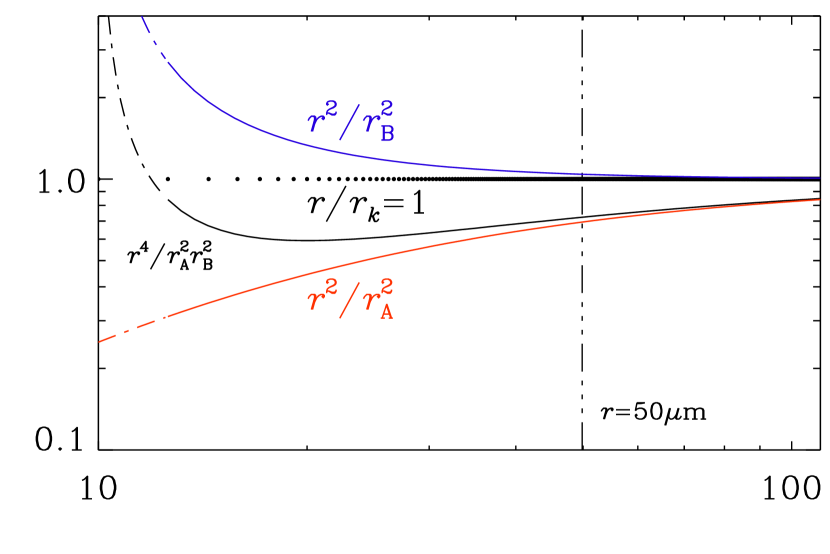
Figure 2: Contributions to the two correction factors $r^{2}/r_{\rm A}^{2}$ (red) and $r^{2}/r_{\rm B}^{2}$ (blue), as well as their product. The dashed-dotted parts of the lines apply to radii smaller than $12.6\,\mu{\rm m}$. The discrete radii $r_{k}$ for $k\geq 2$ are shown in a horizontal line of dots. The vertical dash-triple-dotted line denote the radius $r=50\,\mu{\rm m}$.

In Eq. (13), we have introduced $r_{\rm A}$ and $r_{\rm B}$ to study the effect of relaxing the assumption $r_{\rm A}=r_{\rm B}=r_{k}$, made in simplifying implementations of the LDM. Both of these assumptions are justified at late times when the lucky droplet has become large compared to the smaller ones, but not early on, when the size difference is moderate.

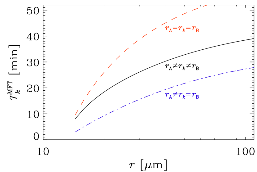
Figure 3: Cumulative mean collision times, $T_{k}^{\rm MFT}$, for $r_{\rm A}\neq r_{k}\neq r_{\rm B}$ (solid black line), compared with the approximations $r_{\rm A}=r_{\rm B}=r_{k}$ (red dashed line) and only $r_{\rm B}=r_{k}$ (blue dash-dotted line).

By comparison, if fluctuations are ignored, the collision times are given by $t_{k}=\lambda_{k}^{-1}$. This is what we refer to as mean-field theory (MFT). In Fig. 3 we demonstrate the effect of the contributions from $r_{\rm A}$ and $r_{\rm B}$ on the mean cumulative collision time in the corresponding MFT,

$$T_{k}^{\rm MFT}=\sum_{k^{\prime}=2}^{k}t_{k^{\prime}}^{\rm MFT},$$ (14)

where

$$t_{k}^{\rm MFT}=\lambda_{k}^{-1}$$ (15)

are the inverse of the mean collision rates. We see that, while the contribution from $r_{\rm A}$ shortens the mean collision time, that of $r_{\rm B}$ enhances it. In Fig. 2, we also see that the contributions to the two correction factors $r^{2}/r_{\rm A}^{2}$ and $r^{2}/r_{\rm B}^{2}$ have opposite trends, which leads to partial cancelation in their product.

In Fig. 4 we show a comparison of the distribution of cumulative collision times for various representations of $r_{k}$. Those are computed numerically using $10^{10}$ realizations of sequences of random collision times $t_{k}$. We refer to appendix A for details of performing this many realizations.

The physically correct model is where $r_{\rm A}\neq r_{k}\neq r_{\rm B}$ (black line in Fig. 4). To demonstrate the sensitivity of $P(T)$ to changes in the representation of $r_{k}$, we show the result for the approximations $r_{\rm A}=r_{k}=r_{\rm B}$ (red line) and $r_{\rm A}\neq r_{k}=r_{\rm B}$ (blue line). The $P(T)$ curve is also sensitive to changes in the collision efficiency late in the evolution. To demonstrate this, we assume $E_{k}\propto r_{k}^{2}$ when $r_{k}$ exceeds a certain arbitrarily chosen value $r_{*}$ between $10$ and $40\,\mu{\rm m}$, and $E_{k}={\rm const}$ below $r_{*}$ (Lamb and Verlinde, 2011). To ensure that $E_{k}\leq 1$, we take

$$E_{k}=E_{*}\,\max\left(1,\,(r_{k}/r_{*})^{2}\right),$$ (16)

with $E_{*}=(r_{*}/50\,\mu{\rm m})^{2}$. However, the normalized $P(T)$ curves are independent of the choice of the value of $E_{*}$. In Fig. 5, we show the results for $r_{\rm A}\neq r_{k}\neq r_{\rm B}$ using $r_{*}=40\,\mu{\rm m}$ and $30\,\mu{\rm m}$ (red and blue lines, respectively) and compare with the case $E_{k}={\rm const}$. The more extreme cases with $r_{*}=20\,\mu{\rm m}$ and $10\,\mu{\rm m}$ are shown as gray lines. The latter is similar to the case $\lambda_{k}\sim r_{k}^{6}$ considered by Kostinski and Shaw (2005) and Wilkinson (2016).

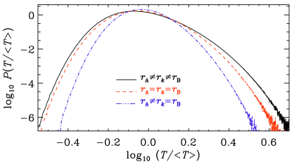
Figure 4: Comparison of $P(T)$ in a double-logarithmic representation for the LDM appropriate to our benchmark (black solid line) with various approximations where $r_{\rm A}=r_{\rm B}=r_{k}$ (red dashed line) along with a case where only $r_{\rm B}=r_{k}$ is assumed (blue dash-dotted line). Here we used $10^{10}$ realizations. Note that we plot the distribution of the cumulative times versus the normalized time, $T/\langle T\rangle$, as was done in the work of Kostinski and Shaw (2005). Normalizing by $\langle T\rangle$ allows us to see changes in the shape of $P(T/\langle T\rangle)$, thus allows a more direct comparison of the subtle differences in the shapes of the different curves and ensures that the peaks of all curves are at approximately the same position.

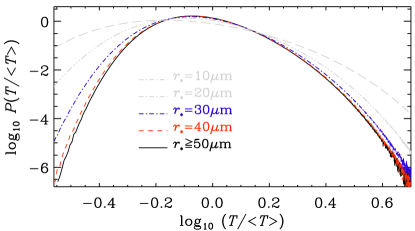
Figure 5: Comparison of $P(T)$ in a double-logarithmic representation for the LDM for $r_{*}=40\,\mu{\rm m}$ and $30\,\mu{\rm m}$ using $r_{\rm A}\neq r_{k}\neq r_{\rm B}$. The black line agrees with that in Fig. 4, and the two gray lines refer to the cases with $r_{*}=20\,\mu{\rm m}$ and $10\,\mu{\rm m}$. Here we used $10^{10}$ realizations.

Table 2: Moments of $X=\ln(T/\langle T\rangle)$ computed from $10^{10}$ realizations for different values of $r_{\ast}$ (in $\mu$m), and different prescriptions of $r_{\rm A}$ and $r_{\rm B}$. The corresponding values of $T_{123}^{\rm MFT}$ are also given and are normalized to unity for $r_{\rm A}\neq r_{k}\neq r_{\rm B}$ with $r_{*}\geq 50\,\mu{\rm m}$.

$r_{\ast}$	$r_{\rm A}$	$r_{\rm B}$	$T_{123}^{\rm MFT}$	$\langle X\rangle$	$\!\sigma(X)\!$	$\!\!\!{\rm skew\ }X\!\!\!$	$\!\!{\rm kurt\ }X\!\!$
—	—	$r_{k}$	0.67	$-0.020$	0.21	​​ 0.22 ​​	​​ $0.08$
—	$r_{k}$	$r_{k}$	1.49	$-0.033$	0.25	​​ 0.25 ​​	​​ $0.05$
—	—	—	1	$-0.040$	0.28	​​ 0.34 ​​	​​ $0.10$
40	—	—	0.99	$-0.041$	0.28	​​ 0.33 ​​	​​ $0.09$
30	—	—	0.93	$-0.046$	0.30	​​ 0.28 ​​	​​ $0.05$
20	—	—	0.79	$-0.063$	0.35	​​ 0.18 ​​	​​ $-0.04$
10	—	—	0.34	$-0.111$	0.47	​​ 0.16 ​​	​​ $-0.17$

When $r_{\rm A}=r_{k}=r_{\rm B}$, or only $r_{k}=r_{\rm B}$, the $P(T)$ curves exhibit smaller widths. By contrast, when the collision efficiency becomes quadratic later on (when $r>r_{*}\equiv 30\,\mu{\rm m}$ or $40\,\mu{\rm m}$), the $P(T)$ curves have larger widths; see Fig. 5. To quantify the shape of $P(T)$, we give in Table 2 the average of $X\equiv\ln(T/\langle T\rangle)$, its standard deviation $\sigma=\langle x^{2}\rangle^{1/2}$, where $x\equiv X-\langle X\rangle$, its skewness ${\rm skew\ }X=\langle x^{3}\rangle/\sigma^{3}$, and its kurtosis ${\rm kurt\ }X=\langle x^{4}\rangle/\sigma^{4}-3$. We recall that, for a perfectly lognormal distribution, ${\rm skew\ }X={\rm kurt\ }X=0$. The largest departure from zero is seen in the skewness, which is positive, indicating that the distribution broadens for large $T$. The kurtosis is rather small, however.

The main conclusion that can be drawn form the investigation mentioned above is that, as far as the shapes of the different curves are concerned, it does not result in any significant error to assume $r_{k}\gg r_{1}$. The value of $\sigma$ is only about 10% smaller if $r_{\rm A}=r_{k}=r_{\rm B}$ is used (compare the red dashed and black solid lines in Fig. 4). This is because the two inaccuracies introduced by $r_{\rm A}$ and $r_{\rm B}$ almost cancel each other. When $r_{*}=40\,\mu{\rm m}$ or $30\,\mu{\rm m}$, for example, the values of $\sigma$ increase by 3% and 15%, respectively; see Table 3, where we also list the corresponding values of $T_{124}^{\rm MFT}$. On the other hand, the actual averages such as $\langle T\rangle\approx T_{124}^{\rm MFT}$ vary by almost 50%.

A straightforward extension of the LDM is to take horizontal variations in the local column density into account. Those are always present for any random initial conditions, but could be larger for turbulent systems, regardless of the droplet speeds. In 3-D superdroplet simulations, large droplets can fall in different vertical columns that contain different numbers of small droplets, a consequence of the fact that the small droplets are initially randomly distributed. To quantify the effect of varying droplet number densities in space, it is necessary to solve for an ensemble of columns with different number densities of the $10\,\mu{\rm m}$ background droplets and compute the distribution of cumulative collision times. These variations lead to a broadening of $P(T)$, but it is a priori not evident how important this effect is. A quantitative analysis is given in appendix C.

3.3 Relation to the superdroplet algorithm

To understand the nature of the superdroplet algorithm, and why it captures the lucky droplet problem accurately, it is important to realize that the superdroplet algorithm is actually a combination of two separate approaches to solving the LDM, each of which turns out to be able to reproduce the lucky droplet problem to high precision. In principle, we can distinguish four different approaches (Table 3) to obtaining the collision time interval $t_{k}$. In approach I, $t_{k}$ was taken from an exponential distribution of random numbers. Another approach is to use a randomly distributed set of $10\,\mu{\rm m}$ background droplets in space and then determine the distance to the next droplet within a vertical cylinder of possible collision partners to find the collision time (approach II). A third approach is to use the mean collision rate to compute the probability of a collision within a fixed time interval. We then use a random number between zero and one (referred to as Monte Carlo method; see, e.g., Sokal, 1997) to decide whether at any time there is a collision or not (approach III). This is actually what is done within each grid cell in the superdroplet algorithm; see Eqs. (3) and (4). The fourth approach is the superdroplet algorithm discussed extensively in section 2.2.1 (approach IV). It is essentially a combination of approaches II and III. We have compared all four approaches and found that they all give very similar results. In the following, we describe approaches II and III in more detail, before focussing on approach IV in section 4.

Table 3: Summary of the four approaches.

Approach ​​	Description
I	time interval $t_{k}$ drawn from distribution
II	primitive Lagrangian particles collide
III	probabilistic, just a pair of superdroplets
IV	superdroplet model (combination of II & III)

3.4 Solving for the collisions explicitly

A more realistic method (approach II; see Table 3) is to compute random realizations of droplet positions in a tall box of size $L_{\rm h}^{2}\times L_{z}$, where $L_{\rm h}$ and $L_{z}$ are the horizontal and vertical extents, respectively. We position the lucky droplet in the middle of the top plane of the box. Collisions are only possible within a vertical cylinder of radius $r_{k}+r_{1}$ below the lucky droplet. Next, we calculate the distance $\Delta z$ to the first collision partner within the cylinder. We assume that both droplets reach their terminal velocity well before the collision. This is an excellent approximation for dilute systems such as clouds, because the droplet response time $\tau_{k}$ of Eq. (2) is much shorter than the mean collision time. Here we use the subscript $k$ to represent the time until the $(k-1)$th collision, which is equivalent to the $i$th droplet. We can then assume the relative velocity between the two as given by the difference of their terminal velocities as

$$\Delta v_{k}=(\tau_{k}-\tau_{1})\,g.$$ (17)

The time until the first collision is then given by $t_{2}=\Delta z/\Delta v_{2}$. This collision results in the lucky droplet having increased its volume by that of the $10\,\mu{\rm m}$ droplet. Correspondingly, the radius of the vertical cylinder of collision partners is also increased. We then search for the next collision partner beneath the position of the first collision, using still the original realization of $10\,\mu{\rm m}$ droplets. We continue this procedure until the lucky droplet reaches a radius of $50\,\mu{\rm m}$. Approach II is an explicit method compared to other approaches listed in Table 3.

3.5 The Monte Carlo method to compute $t_{k}$

In the Monte Carlo method (approach III; see Table 3) we choose a time step $\delta t$ and step forward in time. As in the superdroplet algorithm, the probability of a collision is given by $p_{k}=\lambda_{k}\delta t$; see Eq. (3). We continue until a radius of $50\,\mu{\rm m}$ is reached. We note that in this approach, $n$ is kept constant, i.e., no background droplet is being removed after a collision.

Approach III also allows us to study the effects of jumps in the droplet size by allowing for several lucky droplets at the same time and specifying their collision probability appropriately. These will then be able to interact not only with the $10\,\mu{\rm m}$ background droplets, but they can also collide among themselves, which causes the jumps. We will include this effect in solutions of the LDM using approach III and compare with the results of the superdroplet algorithm.

4 Results

4.1 Accuracy of the superdroplet algorithm

We now want to determine to what extent the fluctuations are correctly represented by the superdroplet algorithm. For this purpose, we now demonstrate the degree of quantitative agreement between approaches I–III and the corresponding solution with the superdroplet algorithm (approach IV; see Table 3). This is done by tracking the growth history of each lucky droplet. As the first few collisions determine the course of the formation of larger droplets, we also use the distribution $P(T)$ of cumulative collision times $T$. We perform $N_{\rm real}$ superdroplet simulations with different random seeds using $\xi_{i}(t_{0})=1$.

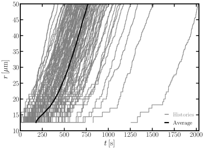
Figure 6: 98 growth histories of lucky droplets obtained from 98 independent 1-D superdroplet simulations (approach IV), as described in the text. All superdroplets have initially the same number of droplets, $\xi_{i}(t_{0})=1$ with $N_{\rm s}(t_{0})=256$. The mean number density of droplets is $n_{0}=3\times 10^{8}\,\rm{m}^{-3}$. The thick solid line shows the average time for each radius.

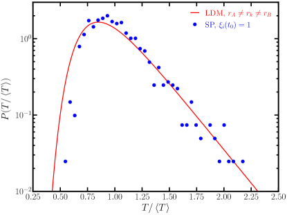
Figure 7: Corresponding $P(T)$ of Fig. 6 obtained with the superdroplet algorithm (blue dots) and the LDM using approach I with $r_{\rm A}\neq r_{k}\neq r_{\rm B}$ (red solid line).

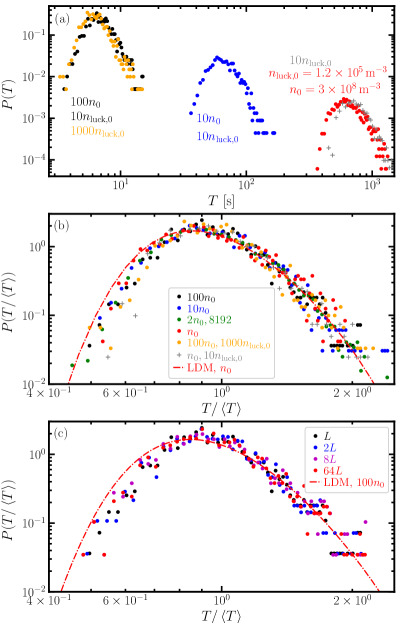
Figure 8: (a): $P(T)$ for $n_{0}$ (red), $10\,n_{0}$ (blue), and $100\,n_{0}$ (black) with $n_{0}=3\times 10^{8}\,\rm{m}^{-3}$ and $L=0.214\,\rm{m}$. In the last case, 0.5% of the background droplets were removed; the orange symbols denote a case with 100 times larger value of $n_{\rm luck}$, where 50% of the background droplets were removed. The gray symbols denote the case of Fig. 7 with ten times more physical lucky droplets ($10\,n_{\rm luck,0}$). (b): $P(T/\langle T\rangle)$ for $n=n_{0}$ (red), $2\,n_{0}$ (green), $10\,n_{0}$ (blue), $100\,n_{0}$ with $10\,n_{\rm luck}$ (black), $1000\,n_{\rm luck}$ (orange), and $n_{0}$ with $10\,n_{\rm luck,0}$ (gray). (c): $P(T/\langle T\rangle)$ for $L$, $2L$, $8L$, and $64L$ with $100\,n_{0}$, obtained using the superdroplet algorithm (approach IV). The red dash-dotted line in (b) represents the LDM (approach I) with $r_{\rm A}\neq r_{k}\neq r_{\rm B}$ and $n_{0}=3\times 10^{8}\,\rm{m}^{-3}$, which is the same simulation as the one in Fig. 7. The green dots in (b) is for 8192 realizations, while all the other simulations are for 1024 realizations.

We begin by looking at growth histories for many individual realizations obtained from the superdroplet simulation. Fig. 6 shows an ensemble of growth histories (thin gray lines) obtained from $N_{\rm real}\approx 10^{3}$ independent simulations, as described above. The times between collisions are random, leading to a distribution of cumulative growth times to reach $50\,\mu{\rm m}$. Also shown is the mean growth curve (thick black line), obtained by averaging the time at fixed radii $r$. This figure demonstrates that the fluctuations are substantial. We also see that large fluctuations relative to the average time are rare.

To quantify the effect of fluctuations from all realizations, we now consider the corresponding $P(T)$ in Fig. 7. We recall that $\xi_{i}(t_{0})=1$ for our superdroplet simulation in Fig. 7. However, a simulation with $\xi_{i}(t_{0})=50$ yields almost the same result; see appendix B.

The comparison of the results for the LDM using approach I and the superdroplet algorithm shows small differences. The width of the $P(T)$ curve is slightly larger for approach I than for the superdroplet simulations. This suggests that the fluctuations, which are at the heart of the LDM, are slightly underrepresented in the superdroplet algorithm. However, this shortcoming may also be a consequence of our choice of having used only 256 superdroplets, i.e., one lucky and 255 background superdroplets. Given that the multiplicities of lucky and background droplets was unity, each collision removed one background droplet. Thus, after 123 collisions, almost $50\%$ of the background droplets were removed by the time the lucky droplet reached $50\,\mu{\rm m}$. Nevertheless, as we will see below, this has only a small effect.

Table 4: Runs of Fig. 8(a), where $n_{i}$ and $n_{i,\rm luck}$ are in units of $n_{i0}=7.5\times 10^{7}\,\rm m^{-3}$, $n$ is in units of $n_{0}=3\times 10^{8}\,\rm m^{-3}$, $n_{\rm luck,0}$ is in units of $1.2\times 10^{5}\,\rm m^{-3}$, using $\delta x^{3}=2.6\times 10^{-8}\,\rm m^{3}$ for all runs, except for the last one (gray), where it is a factor 2 smaller.

color in Fig. 8(a)	red	blue	black	orange	gray
$n_{i}/n_{i0}$	$1$	$10$	$100$	$100$	1
$n_{i,\rm luck}/n_{i0}$	0.1	1	1	100	1
$n/n_{0}$	$1$	$10$	$100$	$100$	1
$n_{\rm luck}/n_{\rm luck,0}$	$1$	$10$	$10$	$1000$	10
$\xi_{\rm back}=\delta x^{3}\,n_{i}$	2	20	200	200	1
$\xi_{\rm luck}=\delta x^{3}\,n_{i,\rm luck}$	0.2	2	2	200	1
removed fraction	$5\%$	$5\%$	$0.5\%$	$50\%$	$50\%$

An important question is to what extent our results depend on the number density of background droplets and the size of the computational domain. To examine this with the superdroplet algorithm (approach IV), we consider three values of the initial number density: $n_{0}=3\times 10^{8}\,\rm m^{-3}$, $10\,n_{0}$, and $100\,n_{0}$, while the initial number density of the lucky droplet is $n_{\rm luck,0}\equiv 1.2\times 10^{5}\,\rm m^{-3}$, $10\,n_{\rm luck,0}$, and again $10\,n_{\rm luck,0}$, respectively; see Table 4 for a summary. Thus, even though the lucky droplet has to collide 123 times to reach $50\,\mu{\rm m}$, it only removes $123\,n_{\rm luck}/n_{0}=5\%$, 5%, and 0.5% of the droplets, respectively. Fig. 8 shows $P(T)$ for these three cases using first the cumulative time $T$ [Fig. 8(a)] and then the normalized time $T/\langle T\rangle$ [Fig. 8(b)]. We see that the positions of the peaks in $P(T)$ change linearly with the initial number density $n_{0}$, but $P(T/\langle T\rangle)$ are very similar to each other. This is related to the fact that, after normalization, $n_{0}$ drops out from the expression for $t_{k}/\langle T\rangle$ in the LDM (approach I); see Eq. (9). At small values of $T/\langle T\rangle$, however, all curves show a similar slight underrepresentation of the fluctuations as already seen in Fig. 7. In all these simulations, we used 1024 realizations, except possibly for one case where we used 8192 realizations; see the green symbols in Fig. 8(b). The distribution of cumulative growth times is obviously much smoother in the latter case, but the overall shape is rather similar.

In the above, the number density of the lucky droplets has been much smaller than the number density of the background droplets. This means that for each collision the physical number of background droplets changed by only a small amount (5% or 0.5%). To see how sensitive our results for $P(T)$ are to this number, we now perform an extra experiment where $50\%$ of the background droplets are removed by the time the lucky droplet reaches $50\,\mu{\rm m}$. This is also shown in Fig. 8(a) and (b); see the orange symbols, where $\xi_{\rm luck}=\xi_{\rm back}=200$. We see that even for 50% removal the results are essentially unchanged.

In our superdroplet simulations (approach IV; see Table 3), the vertical extent of the simulation domain is only $L=0.214\,\rm m$. This is permissible given that we use periodic boundary conditions for the particles. Nevertheless, the accuracy of our results may suffer from poor statistics. To investigate this in more detail, we now perform 1-D simulations with $2L$, $8L$, and $64L$. At the same time, we increased the number of mesh points and the number of superdroplets by the same factors. Since the shape of $P(T/\bar{T})$ is almost independent of $n_{0}$, as shown in Fig. 8(b), we use $n_{0}=3\times 10^{10}\,\rm m^{-3}$ instead of $n_{0}=3\times 10^{8}\,\rm m^{-3}$ to reduce the computational cost. As shown in Fig. 8(c), $P(T/\bar{T})$ is insensitive to the domain size. Therefore, our results with $L=0.214\,\rm m$ can be considered as accurate with respect to $P(T/\bar{T})$.

In the following, we discuss how our conclusions relate to those of earlier work. We then discuss a number of additional factors that can modify the results. Those additional factors can also be taken into account in the LDM. Even in those cases, it turns out that the differences between the LDM and the superdroplet algorithm are small.

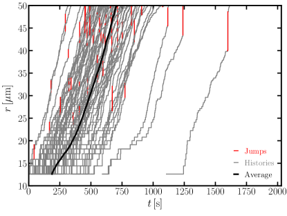
Figure 9: Same as Fig. 6 but with initial condition $\xi_{i}(t_{0})=2$ using $N_{\rm s}(t_{0})=128$, corresponding to the same number of physical droplets as in Fig. 6, where $\xi_{i}(t_{0})=1$. Note the occurrence of jumps, indicated in red.

4.2 The occurrence of jumps

One of the pronounced features in our superdroplet simulations with $\xi_{i}(t_{0})>1$ is the possibility of jumps. We see examples in Fig. 9 where $\xi_{\rm luck}=\xi_{\rm back}=2$ and the jumps are visualized by the red vertical lines. Those jumps are caused by the coagulation of the lucky droplet with droplets of radii larger than $10\,\mu{\rm m}$ that were the result of other lucky droplets in the simulations. What is the effect of these jumps? Could they be responsible for the behavior found by Dziekan and Pawlowska (2017) that the difference in their $t_{10\%}$ between the numerical and theoretical calculation decreases with the square root of the number of physical droplets, as we discussed in section 1?

It is clear that those jumps occur mainly during the last few steps of a lucky droplet growing to $50\,\mu{\rm m}$ (see Fig. 9) when there has been enough time to grow several more lucky droplets. Because the collision times are so short at late times, the jumps are expected to be almost insignificant. To quantify this, it is convenient to use approach III, where we choose $N_{\rm s}^{\rm(luck)}=3$ superdroplets simultaneously. (As always in approach III, the background particles are still represented by only one superdroplet, and $n$ is kept constant.) We also choose $\xi_{\rm luck}=1$, and therefore $N_{\rm d}^{\rm(luck)}=3$. The lucky droplets can grow through collisions with the $10\,\mu{\rm m}$ background droplets and through mutual collisions between lucky droplets. The collision rate between lucky droplets $i$ and $j$ is, analogously to Eq. (12), given by

$$\lambda_{ij}^{\rm(luck)}=\pi\left(r_{i}+r_{j}\right)^{2}|\mbox{\boldmath$v$}_{i}-\mbox{\boldmath$v$}_{j}|\;n_{\rm luck},$$ (18)

where $n_{\rm luck}$ is the number density of physical droplets in the superdroplet representing the lucky droplet. To obtain an expression for $n_{\rm luck}$ in terms of the volume of a grid cell $\delta x^{3}$, we write $n_{\rm luck}=\xi_{\rm luck}/\delta x^{3}$. The ratio of the physical number of lucky droplets, $N_{\rm d}^{\rm(luck)}$, to the physical number of background droplets, $N_{\rm d}^{\rm(back)}$ is given by

$$\epsilon=\frac{N_{\rm d}^{\rm(luck)}}{N_{\rm d}^{\rm(back)}}=\frac{\xi_{\rm luck}\,N_{\rm s}^{\rm(luck)}}{\xi_{\rm back}\,N_{\rm s}^{\rm(back)}}.$$ (19)

To investigate the effect of jumps on $P(T)$ in the full superdroplet model studied above (see Figs. 6 and 9), we first consider the case depicted in Fig. 6, where $\xi_{\rm luck}=\xi_{\rm back}\equiv\xi_{i}(t_{0})=1$. Here, we used $N_{\rm s}=256$ superdroplets, of which one contained the lucky droplet, so $N_{\rm s}^{\rm(luck)}=1$, and the other 255 superdroplets contained a $10\,\mu{\rm m}$ background droplet each. In our superdroplet solution, the ratio (19) was therefore $\epsilon\approx 1/255=0.004$. Using approach III, $\epsilon$ enters simply as an extra factor in the collision probability between different lucky droplets. (In approach III, all quantities in Eq. (19) are kept constant.) The effect on $P(T)$ is shown in Fig. 10, where we present the cumulative collision times for models with three values of $\epsilon$ using approach III. We see that for small values of $\epsilon$, the cumulative distribution function is independent of $\epsilon$, and the effect of jumps is therefore negligible (compare the black solid and the red dashed lines of Fig. 10). More significant departures due to jumps can be seen when $\epsilon=0.02$ and larger.

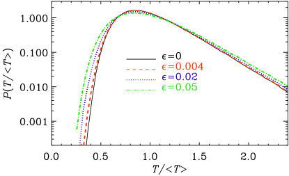
Figure 10: Comparison of models with $\epsilon=0$ (no jumps), 0.004 (the value expected for the simulations), 0.02, and 0.05 using approach III; see Table 3.

Let us now compare with the case in which we found jumps using the full superdroplet approach (approach IV). The jumps in the growth histories cause the droplets to grow faster than without jumps. However, jumps do not have a noticeable effect upon $P(T)$ in the superdroplet simulations we conducted; see Fig. 11. By comparing $P(T)$ for $\xi_{\rm back}=40$ (blue crosses in Fig. 11) with that for $\xi_{\rm back}=2$ (black circles), while keeping $\xi_{\rm luck}=2$ in both cases, hardly any jumps occur and the lucky droplet result remains equally accurate.

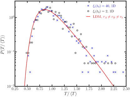
Figure 11: $P(T/\langle T\rangle)$ of simulations in Fig. 9 (black circles) and the ones with initially $\xi_{\rm back}=40$ (blue crosses). $\xi_{\rm luck}=2$ in both cases. The red line denotes the LDM (approach I) with $r_{\rm A}\neq r_{k}\neq r_{\rm B}$, which is the same simulation as the one in Fig. 7.

For larger values of $\epsilon$, jumps occur much earlier, as can be seen from Fig. 12, where we show 30 growth curves for the cases $\epsilon=0.004$, which is relevant to the simulations of Fig. 7, as well as $\epsilon=0.02$, and 0.05. We also see that for large values of $\epsilon$, the width in the distribution of arrival times is broader and that both shorter and longer times are possible. This suggests that the reason for the finite residual error in the values of $t_{10\%}$ found by Dziekan and Pawlowska (2017) for $\xi_{i}(t_{0})>9$ could indeed be due to jumps. In our superdroplet simulations, by contrast, jumps cannot occur when $\xi_{i}(t_{0})=1$ or $\xi_{\rm back}\gg\xi_{\rm luck}$.

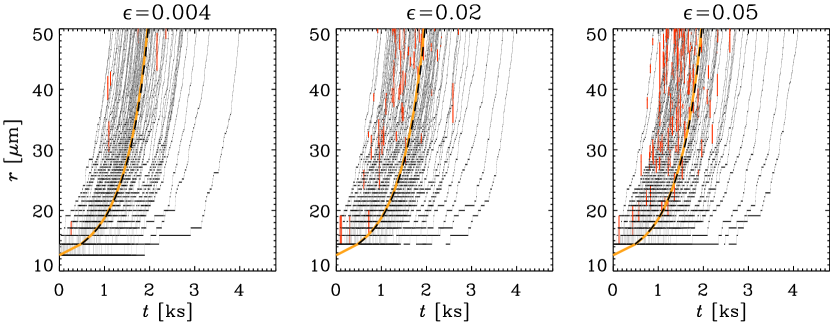
Figure 12: Growth histories from approach III for $\epsilon=0.004$ (very few jumps, relevant to the simulations of Fig. 7), as well as $\epsilon=0.02$, and 0.05, where jumps are more frequent. The orange thick solid line gives the average collision time and agrees with that of MFT (thick black dashed line) within about a percent.

4.3 The two aspects of randomness

Let us now quantify the departure that is caused by the use of the Monte Carlo collision scheme. To do this, we need to assess the effects of randomness introduced through Eqs. (3) and (4) on the one hand and the random distribution of the $10\,\mu{\rm m}$ background droplets on the other. Both aspects enter in the superdroplet algorithm.

We recall that in approach II, fluctuations originate solely from the random distribution of the $10\,\mu{\rm m}$ background droplets. In approach III, on the other hand, fluctuations originate solely from the Monte Carlo collision scheme. By contrast, approach I is different from either of the two, because it just uses the exponential distribution of the collision time intervals, which is indirectly reproduced by the random initial droplet distribution in approach II and by the Monte Carlo scheme in approach III.

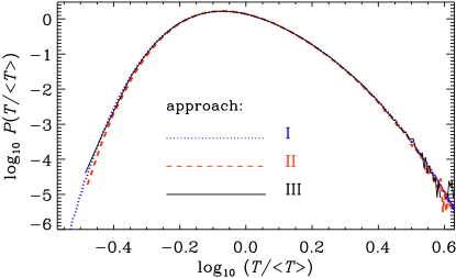
Figure 13: Comparison of $P(T)$ for approaches I, II, and III.

Table 5: Comparison of the moments of $X=\ln(T/\langle T\rangle)$ for approaches I–III.

Approach	$\langle X\rangle$	$\sigma(X)$	${\rm skew\ }X$	${\rm kurt\ }X$
I	$-0.040$	0.279	0.34	$0.10$
II	$-0.039$	0.275	0.35	$0.11$
III	$-0.040$	0.279	0.34	$0.11$

In Fig. 13, we compare approaches I, II, and III. For our solution using approach II, we use a nonperiodic domain of size $10^{-4}\times 10^{-4}\times 700\,\rm m^{3}$, thus containing on average 2100 droplets. This was tall enough for the lucky droplet to reach $50\,\mu{\rm m}$ for all the $10^{7}$ realizations in this experiment. The differences between them are very minor, and also the first few moments are essentially the same; see Table 5. We thus see good agreement between the different approaches. This suggests that the fluctuations introduced through random droplet positions is not crucial and that it can be substituted by the fluctuations of the Monte Carlo scheme alone.

It is worth noting that we were able to perform $10^{7}$ and $10^{6}$ realizations with approaches II and III, respectively, and $10^{10}$ realizations with approach I, while in the superdroplet algorithm (approach IV), we could only run $10^{3}$–$10^{4}$ realizations due to the limitation of the computational power. This may be the reason why fluctuations appear to be slightly underrepresented in the superdroplet algorithm; see Fig. 7 and the discussion in section 4.4.1. Nevertheless, the agreement between the LDM and the superdroplet simulations demonstrates that the superdroplet algorithm is able to represent fluctuations during collisions and does not contain mean-field elements. This can be further evidenced by the fact that the results of approaches II and III agree perfectly with those of approach I, and the superdroplet algorithm is just the combination of approaches II and III.

5 Discussion

Fluctuations play a central role in the LDM. We have therefore used it as a benchmark for our simulation. It turns out that the superdroplet algorithm is able to reproduce the growth histories qualitatively and the distribution of cumulative collision times quantitatively. The role of fluctuations was also investigated by Dziekan and Pawlowska (2017), whose approach to assessing the fluctuations is different from ours. Instead of analyzing the distribution of cumulative collision times, as we do here, their primary diagnostics is the time $t_{10\%}$, after which 10% of the mass of cloud droplets has reached a radius of $40\,\mu{\rm m}$. In the LDM, such a time would be infinite, because there is only one droplet that is allowed to grow. They then determined the accuracy with which the value of $t_{10\%}$ is determined. The accuracy increases with the square root of the number of physical droplets, provided that the ratio $\xi_{i}(t_{0})$ is kept below a limiting value of about 9. For $\xi_{i}(t_{0})>9$, they found that there is always a residual error in the value of $t_{10\%}$ that no longer diminishes as they increase the number of physical droplets. We have demonstrated that, when $\xi_{i}(t_{0})>1$, jumps in the growth history tend to occur. Those jumps can lead to shorter cumulative collision times, which could be the source of the residual error they find.

For a given fraction of droplets that first reach a size of $40\,\mu{\rm m}$, they also determined their average cumulative collision time. They found a significant dependence on the number of physical droplets. This is very different in our case where we just have to make sure that the number of superdroplets is large enough to keep finding collision partners in the simulations. However, as the authors point out, this is a consequence of choosing an initial distribution of droplet sizes that has a finite width. This implies that for a larger number of droplets, there is a larger chance that there could be a droplet that is more lucky than for a model with a smaller number of droplets. In our case, by contrast, we always have a well-known number of superdroplets of exactly $12.6\,\mu{\rm m}$, which avoids the sensitivity on the number of droplets.

The $\xi_{i}(t_{0})=9$ limit of Dziekan and Pawlowska (2017) does not hold in this investigation. In this context we need to recall that their criterion for acceptable quality concerned the relative error of the time in which 10% of the total water has been converted to $40\,\mu{\rm m}$ droplets. In our case, we have focussed on the shape of the $P(T)$ curve, especially for small $T$.

6 Conclusions

We investigated the growth histories of droplets settling in quiescent air using superdroplet simulations. The goal was to determine how accurately these simulations represent the fluctuations of the growth histories. This is important because the observed formation time of drizzle-sized droplets is much shorter than the one predicted based on the mean collisional cross section. The works of Telford (1955), Kostinski and Shaw (2005), and Wilkinson (2016) have shown that this discrepancy can be explained by the presence of stochastic fluctuations in the time intervals between droplet collisions. By comparing with the lucky droplet model (LDM) quantitatively, we have shown that the superdroplet simulations capture the effect of fluctuations.

A tool to quantify the significance of fluctuations on the growth history of droplets is the distribution of cumulative collision times. Our results show that the superdroplet algorithm reproduces the distribution of cumulative collision times that is theoretically expected based on the LDM. However, the approximation of representing the dependence of the mean collision rate on the droplet radius by a power law is not accurate and must be relaxed for a useful benchmark experiment.

In summary, the superdroplet algorithm appears to take fluctuations fully into account, at least for the problem of coagulation due to gravitational settling in quiescent air. Computing the distribution of cumulative collision times in the context of turbulent coagulation would be rather expensive, because one would need to perform many hundreds of fully resolved 3-D simulations. Our study suggests that fluctuations are correctly described for collisions between droplets settling in quiescent fluid, but we do not know whether this conclusion carries over to the turbulent case.

Appendix A Numerical treatment of approach I

In section 3.2, we noted that solutions to approach I have been obtained with the Pencil Code (Pencil Code Collaboration et al., 2021). This might seem somewhat surprising, given that this code is primarily designed for solving partial differential equations. It should be realized, however, that this code also provides a flexible framework for using the message passing interface, data analysis such as the computation of probability density distributions, and input/output.

To compute the probability distribution of $T$ with approach I, we need to sum up sequences of random numbers for many independent realizations of $t_{k}$ drawn from an exponential distribution. We use the special/lucky_droplet module provided with the code. Each point in the computational domain corresponds to an independent realization, so each point is initialized with a different random seed. The domain is divided into 1024 smaller domains, allowing the computational tasks to be performed simultaneously on 1024 processors, which takes about $4\min$ on a Cray XC40.

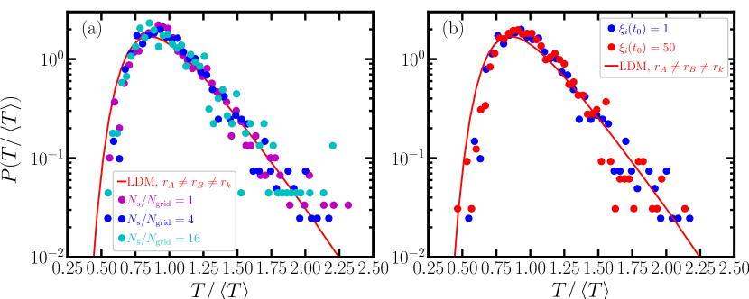
Figure 14: Comparison of $P(T)$ for (a) different $N_{\rm s}/N_{\rm grid}$ with fixed $\xi_{i}(t_{0})=1$ and (b) for different $\xi_{i}(t_{0})$ with fixed $N_{\rm s}/N_{\rm grid}=4$. The blue dots represent $P(T/\langle T\rangle)$ from the simulation as in Fig. 7. The red curve shows the result for the LDM (approach I) with $r_{\rm A}\neq r_{\rm B}\neq r_{k}$, which is the same simulation as the one in Fig. 7.

Appendix B Dependence on initial $N_{\rm s}/N_{\rm grid}$ and $N_{\rm d}/N_{\rm s}$

In this appendix, we first test the statistical convergence of $P(T)$ for the initial number of superdroplets per grid cell, $N_{\rm s}(t_{0})/N_{\rm grid}$. As discussed in section 2.2.2, we set $N_{\rm s}(t_{0})/N_{\rm grid}=4$ for 1-D simulations. Using the same numerical setup, we examine the statistical convergence of $P(T)$ for different values of $N_{\rm s}(t_{0})/N_{\rm grid}$. As shown in Fig. 14(a), $P(T)$ converges even at $N_{\rm s}(t_{0})/N_{\rm grid}=1$. This is important because one can use as few superdroplets as possible once $N_{\rm grid}$ is fixed, without suffering from the statistical fluctuations.

The most practical application of the superdroplet algorithm is the case when $\xi^{i}\geq 1$. Thus, we investigate how $\xi$ affects fluctuations by performing the same 1-D simulation as described in section 2.2.2 with different values of $\xi^{i}(t_{0})$. Fig. 14(b) shows that $P(T)$ is insensitive to $\xi^{i}(t_{0})$, which suggests that the superdroplet algorithm can capture the effects of fluctuations regardless of the value of $\xi^{i}(t_{0})$. This is different from Dziekan and Pawlowska (2017), who found that the approach can represent fluctuations only if $N_{\rm d}(t_{0})/N_{\rm s}(t_{0})\leq 9$.

Appendix C Horizontal variations of droplet densities

In this appendix, we analyze in more detail the effect of horizontal variations of droplet densities discussed section 3.2. This is relevant for computing the 3-D distribution function from a 1-D distribution function. The LDM applies to a given value of the number density. Other columns have somewhat different number densities and therefore also different mean cumulative collision times. The LDM with approaches I–III can be extended to include this effect by computing cases with different number densities and then combining $P(T)$ and normalizing by the $\langle T\rangle$ for the combined $P(T)$. This can be formulated by introducing the column density as

$$\Sigma(x,y)=\int_{z_{1}}^{z_{2}}n(x,y,z)\,{\rm d}z,$$ (20)

where $z_{1}$ and $z_{2}$ denote the vertical slab in which the first collision occurs, and using this $\Sigma(x,y)$ as a weighting factor for the 1-D distribution functions $P^{\rm 1D}(T)$ to compute the 3-D distribution functions as

$$P^{\rm 3D}(T)=\left.\int\Sigma(x,y)P^{\rm 1D}(T)\,{\rm d}x\,{\rm d}y\;\right/\!\!\int\Sigma(x,y)\,{\rm d}x\,{\rm d}y.$$ (21)

Since the first collision matters the most, we choose $z_{2}=z_{\max}$ (where the lucky droplet is released) and $z_{1}=z_{\max}-v_{2}/\lambda_{2}$ (where it has its first collision).

Table 6: Results for approach II using 30,000 realization showing the effects of horizontal density fluctuations in 3-D, and comparison with MFT.

Composition	$\delta n_{\rm rms}/n_{0}$	$\delta n_{\max}/n_{0}$	$T_{\min}$ [s]	$T_{\rm MFT}$ [s]	$\langle T(n_{\max})\rangle$ [s]	$\langle T\rangle$ [s]	$T_{\min}/\langle T\rangle$	$T_{P=0.01}/\langle T\rangle$
(0)	0	0	782	1969	2117	2117	0.37	0.44
(i)	0.08	0.10	795	1790	1923	2126	0.37	0.42
(ii)	0.14	0.20	767	1641	1758	2155	0.36	0.40
(iii)	0.20	0.30	631	1515	1628	2203	0.29	0.36

Our reference model had a number density of $n_{0}=10^{8}\,\rm m^{-3}$. We now consider compositions of models with different values, where we include the densities (i) $0.9\times 10^{8}\,\rm m^{-3}$ and $1.1\times 10^{8}\,\rm m^{-3}$, as well as (ii) $0.8\times 10^{8}\,\rm m^{-3}$ and $1.2\times 10^{8}\,\rm m^{-3}$, and finally also (iii) $0.7\times 10^{8}\,\rm m^{-3}$ and $1.3\times 10^{8}\,\rm m^{-3}$. All these compositions have the same mean droplet number density but different distributions around the mean. We first average the distribution function and then normalize with respect to the mean collision time for the ensemble over all columns. The parameters of the resulting distributions are listed in Table 6 for three compositions with different density dispersions. We see that, as we move from composition (i) to compositions (ii) and (iii), the dispersion ($\delta n_{\rm rms}/n_{0}$) increases from 0.08 to 0.14 and 0.20, the distribution $P(T)$ extends further to both the left and right. The reference model is listed as (o). Here we give the rms value of the column-averaged densities, $\langle n\rangle_{i}$, as

$$\delta n_{\rm rms}=\left[\sum_{i=0}^{N_{i}}\left(\langle n\rangle_{i}^{2}-n_{0}^{2}\right)\right]^{1/2},$$ (22)

where $i$ denotes the column and $N_{i}$ is the number of columns. We also give the maximum difference from the average density,

$$\delta n_{\max}=\max_{i}\left(\langle n\rangle_{i}-n_{0}\right),$$ (23)

for families (i) with $N_{i}=2$, (ii) with $N_{i}=4$, and (iii) with $N_{i}=6$. We also list in Table 6 several characteristic times in seconds. The quantity $T_{\min}$ is the shortest time in which the lucky droplet reaches $50\,\mu{\rm m}$, $T_{\rm MFT}$ denotes the value based on MFT, $\langle T(n_{\max})\rangle$ is the mean value based on the column with maximum droplet density and $\langle T\rangle$ is the mean based on all columns. It turns out that for the models of all three families, the value of $T_{\min}$ agrees with that obtained solely from the model with the highest density, which is $1.3\times 10^{8}\,\rm m^{-3}$ for composition (ii), for example.

The quantity $\langle T(n_{\max})\rangle$, i.e., the average time for all of the columns with the largest density, is shorter than the $\langle T\rangle$ for all the columns, especially for composition (iii) where the largest densities occur. For the model (o), there is only one column, so $\langle T(n_{\max})\rangle$ is the same as $\langle T\rangle$. The value $T_{\rm MFT}$ based on MFT is always somewhat shorter than $\langle T(n_{\max})\rangle$. Finally, we give in Table 6 the ratios $T_{\min}/\langle T\rangle$ and $T_{P=0.01}/\langle T\rangle$, where the subscript $P=0.01$ indicates the argument of $P(T)$ where the function value is 0.01.

References

- Arabas and Shima (2013) Arabas, A., and S. Shima, 2013: Large-eddy simulations of trade wind cumuli using particle-based microphysics with monte carlo coalescence. Journal of the Atmospheric Sciences, 70 (9), 2768–2777, 10.1175/JAS-D-12-0295.1.
- Baehr and Klahr (2019) Baehr, H., and H. Klahr, 2019: The concentration and growth of solids in fragmenting circumstellar disks. The Astrophysical Journal, 881 (2), 162, 10.3847/1538-4357/ab2f85.
- Brdar and Seifert (2018) Brdar, S., and A. Seifert, 2018: Mcsnow: A monte-carlo particle model for riming and aggregation of ice particles in a multidimensional microphysical phase space. Journal of Advances in Modeling Earth Systems, 10 (1), 187–206, 10.1002/2017MS001167.
- Drakowska et al. (2014) Drakowska, J., F. Windmark, and C. P. Dullemond, 2014: Modeling dust growth in protoplanetary disks: The breakthrough case. Astronomy & Astrophysics, 567, A38, 10.1051/0004-6361/201423708, 1406.0870.
- Dziekan and Pawlowska (2017) Dziekan, P., and H. Pawlowska, 2017: Stochastic coalescence in lagrangian cloud microphysics. Atmospheric Chemistry and Physics, 17 (22), 13 509–13 520, 10.5194/acp-17-13509-2017.
- Dziekan et al. (2019) Dziekan, P., M. Waruszewski, and H. Pawlowska, 2019: University of Warsaw Lagrangian Cloud Model (UWLCM) 1.0: a modern large-eddy simulation tool for warm cloud modeling with Lagrangian microphysics. Geoscientific Model Development, 12 (6), 2587–2606, 10.5194/gmd-12-2587-2019.
- Gillespie (1972) Gillespie, D. T., 1972: The stochastic coalescence model for cloud droplet growth. Journal of the Atmospheric Sciences, 29 (8), 1496–1510, 10.1175/1520-0469(1972)029<1496:tscmfc>2.0.co;2.
- Grabowski (2020) Grabowski, W. W., 2020: Comparison of Eulerian Bin and Lagrangian Particle-Based Microphysics in Simulations of Nonprecipitating Cumulus. Journal of Atmospheric Sciences, 77 (11), 3951–3970, 10.1175/JAS-D-20-0100.1.
- Grabowski et al. (2019) Grabowski, W. W., H. Morrison, S.-I. Shima, G. C. Abade, P. Dziekan, and H. Pawlowska, 2019: Modeling of cloud microphysics: Can we do better? Bulletin of the American Meteorological Society, 100 (4), 655–672, 10.1175/BAMS-D-18-0005.1.
- Hoffmann et al. (2019) Hoffmann, F., T. Yamaguchi, and G. Feingold, 2019: Inhomogeneous mixing in Lagrangian cloud models: Effects on the production of precipitation embryos. Journal of the Atmospheric Sciences, 76 (1), 113–133, 10.1175/JAS-D-18-0087.1.
- Jaruga and Pawlowska (2018) Jaruga, A., and H. Pawlowska, 2018: libcloudph++ 2.0: aqueous-phase chemistry extension of the particle-based cloud microphysics scheme. Geoscientific Model Development, 11 (9), 3623–3645, 10.5194/gmd-11-3623-2018.
- Johansen et al. (2015) Johansen, A., M.-M. Mac Low, P. Lacerda, and M. Bizzarro, 2015: Growth of asteroids, planetary embryos, and kuiper belt objects by chondrule accretion. Science Advances, 1 (3), e1500 109, 10.1126/sciadv.1500109.
- Johansen et al. (2012) Johansen, A., A. N. Youdin, and Y. Lithwick, 2012: Adding particle collisions to the formation of asteroids and Kuiper belt objects via streaming instabilities. Astron, Astroph., 537, A125, 10.1051/0004-6361/201117701.
- Kobayashi et al. (2019) Kobayashi, H., K. Isoya, and Y. Sato, 2019: Importance of giant impact ejecta for orbits of planets formed during the giant impact era. The Astrophysical Journal, 887 (2), 226, 10.3847/1538-4357/ab5307.
- Kostinski and Shaw (2005) Kostinski, A. B., and R. A. Shaw, 2005: Fluctuations and luck in droplet growth by coalescence. Bull. Am. Met. Soc., 86, 235–244, 10.1175/BAMS-86-2-235.
- Lamb and Verlinde (2011) Lamb, D., and J. Verlinde, 2011: Growth by collection, 380–414. Cambridge University Press, 10.1017/CBO9780511976377.
- Li et al. (2017) Li, X.-Y., A. Brandenburg, N. E. L. Haugen, and G. Svensson, 2017: Eulerian and Lagrangian approaches to multidimensional condensation and collection. J. Adv. Modeling Earth Systems, 9, 1116–1137, 10.1002/2017MS000930.
- Li et al. (2018) Li, X.-Y., A. Brandenburg, G. Svensson, N. E. Haugen, B. Mehlig, and I. Rogachevskii, 2018: Effect of turbulence on collisional growth of cloud droplets. Journal of the Atmospheric Sciences, 75 (10), 3469–3487, 10.1175/JAS-D-18-0081.1.
- Li et al. (2020) Li, X.-Y., A. Brandenburg, G. Svensson, N. E. Haugen, B. Mehlig, and I. Rogachevskii, 2020: Condensational and collisional growth of cloud droplets in a turbulent environment. Journal of the Atmospheric Sciences, 77 (1), 337–353, 10.1175/JAS-D-19-0107.1.
- Li and Mattsson (2020) Li, X.-Y., and L. Mattsson, 2020: Dust growth by accretion of molecules in supersonic interstellar turbulence. The Astrophysical Journal, 903 (2), 148, 10.3847/1538-4357/abb9ad.
- Li and Mattsson (2021) Li, X.-Y., and L. Mattsson, 2021: Coagulation of inertial particles in supersonic turbulence. Astronomy & Astrophysics, 648, A52, 10.1051/0004-6361/202040068.
- Li et al. (2019) Li, X.-Y., G. Svensson, A. Brandenburg, and N. E. L. Haugen, 2019: Cloud-droplet growth due to supersaturation fluctuations in stratiform clouds. Atmospheric Chemistry and Physics, 19 (1), 639–648, 10.5194/acp-19-639-2019.
- Madival (2018) Madival, D. G., 2018: Stochastic growth of cloud droplets by collisions during settling. Theoretical and Computational Fluid Dynamics, 32 (2), 235–244, 10.1007/s00162-017-0451-z.
- Naumann and Seifert (2015) Naumann, A. K., and A. Seifert, 2015: A Lagrangian drop model to study warm rain microphysical processes in shallow cumulus. Journal of Advances in Modeling Earth Systems, 7 (3), 1136–1154, 10.1002/2015MS000456.
- Naumann and Seifert (2016) Naumann, A. K., and A. Seifert, 2016: Recirculation and growth of raindrops in simulated shallow cumulus. Journal of Advances in Modeling Earth Systems, 8 (2), 520–537, 10.1002/2016MS000631.
- Nesvornỳ et al. (2019) Nesvornỳ, D., R. Li, A. N. Youdin, J. B. Simon, and W. M. Grundy, 2019: Trans-Neptunian binaries as evidence for planetesimal formation by the streaming instability. Nature Astronomy, 3 (9), 808–812, 10.1038/s41550-019-0806-z.
- Onishi et al. (2015) Onishi, R., K. Matsuda, and K. Takahashi, 2015: Lagrangian tracking simulation of droplet growth in turbulence–turbulence enhancement of autoconversion rate. Journal of the Atmospheric Sciences, 72 (7), 2591–2607, 10.1175/JAS-D-14-0292.1.
- Ormel et al. (2009) Ormel, C., D. Paszun, C. Dominik, and A. Tielens, 2009: Dust coagulation and fragmentation in molecular clouds-I. How collisions between dust aggregates alter the dust size distribution. Astronomy & Astrophysics, 502 (3), 845–869, 10.1051/0004-6361/200811158.
- Paoli et al. (2004) Paoli, R., J. Helie, and T. Poinsot, 2004: Contrail formation in aircraft wakes. Journal of Fluid Mechanics, 502, 361–373, 10.1017/S0022112003007808.
- Pencil Code Collaboration et al. (2021) Pencil Code Collaboration, and Coauthors, 2021: The Pencil Code, a modular MPI code for partial differential equations and particles: multipurpose and multiuser-maintained. The Journal of Open Source Software, 6 (58), 2807, 10.21105/joss.02807, 2009.08231.
- Poon et al. (2020) Poon, S. T., R. P. Nelson, S. A. Jacobson, and A. Morbidelli, 2020: Formation of compact systems of super-Earths via dynamical instabilities and giant impacts. Monthly Notices of the Royal Astronomical Society, 491 (4), 5595–5620, 10.1093/mnras/stz3296.
- Pruppacher and Klett (1997) Pruppacher, H. R., and J. D. Klett, 1997: Microphysics of clouds and precipitation, 2nd edition. Kluwer Academic Publishers, Dordrecht, The Nederlands, 10.1080/02786829808965531, 954p.
- Riechelmann et al. (2012) Riechelmann, T., Y. Noh, and S. Raasch, 2012: A new method for large-eddy simulations of clouds with Lagrangian droplets including the effects of turbulent collision. New Journal of Physics, 14 (6), 065 008, 10.1088/1367-2630/14/6/065008.
- Ros and Johansen (2013) Ros, K., and A. Johansen, 2013: Ice condensation as a planet formation mechanism. Astronomy & Astrophysics, 552, A137, 10.1051/0004-6361/201220536.
- Ros et al. (2019) Ros, K., A. Johansen, I. Riipinen, and D. Schlesinger, 2019: Effect of nucleation on icy pebble growth in protoplanetary discs. Astronomy & Astrophysics, 629, A65, 10.1051/0004-6361/201834331.
- Saffman and Turner (1956) Saffman, P. G., and J. S. Turner, 1956: On the collision of drops in turbulent clouds. Journal of Fluid Mechanics, 1, 16–30, 10.1017/S0022112056000020.
- Saito and Gotoh (2018) Saito, I., and T. Gotoh, 2018: Turbulence and cloud droplets in cumulus clouds. New Journal of Physics, 20 (2), 023 001, 10.1088/1367-2630/aaa229.
- Sato et al. (2017) Sato, Y., S.-i. Shima, and H. Tomita, 2017: A grid refinement study of trade wind cumuli simulated by a Lagrangian cloud microphysical model: the super-droplet method. Atmospheric Science Letters, 18 (9), 359–365, 10.1002/asl.764.
- Sato et al. (2018) Sato, Y., S.-i. Shima, and H. Tomita, 2018: Numerical convergence of shallow convection cloud field simulations: Comparison between double-moment Eulerian and particle-based Lagrangian microphysics coupled to the same dynamical core. Journal of Advances in Modeling Earth Systems, 10 (7), 1495–1512, 10.1029/2018MS001285.
- Seifert et al. (2019) Seifert, A., J. Leinonen, C. Siewert, and S. Kneifel, 2019: The geometry of rimed aggregate snowflakes: A modeling study. Journal of Advances in Modeling Earth Systems, 11 (3), 712–731, 10.1029/2018MS001519.
- Shima et al. (2009) Shima, S., K. Kusano, A. Kawano, T. Sugiyama, and S. Kawahara, 2009: The super-droplet method for the numerical simulation of clouds and precipitation: a particle-based and probabilistic microphysics model coupled with a non-hydrostatic model. Quart. J. Roy. Met. Soc., 135, 1307–1320, 10.1002/qj.441, physics/0701103.
- Shima et al. (2020) Shima, S.-i., Y. Sato, A. Hashimoto, and R. Misumi, 2020: Predicting the morphology of ice particles in deep convection using the super-droplet method: development and evaluation of SCALE-SDM 0.2. 5-2.2. 0,-2.2. 1, and-2.2. 2. Geoscientific Model Development, 13 (9), 4107–4157, 10.5194/gmd-13-4107-2020.
- Sokal (1997) Sokal, A., 1997: Monte Carlo Methods in Statistical Mechanics: Foundations and New Algorithms. Boston: Springer, 10.1007/978-1-4899-0319-8_6.
- Sölch and Kärcher (2010) Sölch, I., and B. Kärcher, 2010: A large-eddy model for cirrus clouds with explicit aerosol and ice microphysics and Lagrangian ice particle tracking. Quarterly Journal of the Royal Meteorological Society, 136 (653), 2074–2093, 10.1002/qj.689.
- Telford (1955) Telford, J. W., 1955: A new aspect of coalescence theory. Journal of Meteorology, 12 (5), 436–444, 10.1175/1520-0469(1955)012<0436:anaoct>2.0.co;2.
- Twomey (1964) Twomey, S., 1964: Statistical effects in the evolution of a distribution of cloud droplets by coalescence. Journal of the Atmospheric Sciences, 21 (5), 553–557, 10.1175/1520-0469(1964)021<0553:seiteo>2.0.co;2.
- Unterstrasser et al. (2017) Unterstrasser, S., F. Hoffmann, and M. Lerch, 2017: Collection/aggregation algorithms in Lagrangian cloud microphysical models: rigorous evaluation in box model simulations. Geoscientific Model Development, 10 (4), 1521–1548, 10.5194/gmd-10-1521-2017.
- Unterstrasser et al. (2020) Unterstrasser, S., F. Hoffmann, and M. Lerch, 2020: Collisional growth in a particle-based cloud microphysical model: insights from column model simulations using LCM1D (v1. 0). Geoscientific Model Development, 13 (11), 5119–5145, 10.5194/gmd-13-5119-2020.
- Wilkinson (2016) Wilkinson, M., 2016: Large deviation analysis of rapid onset of rain showers. Physics Review Letters, 116, 018 501, 10.1103/PhysRevLett.116.018501.
- Yang and Zhu (2020) Yang, C.-C., and Z. Zhu, 2020: Morphological signatures induced by dust back reaction in discs with an embedded planet. Monthly Notices of the Royal Astronomical Society, 491 (4), 4702–4718, 10.1093/mnras/stz3232.
- Zannetti (1984) Zannetti, P., 1984: New monte carlo scheme for simulating lagranian particle diffusion with wind shear effects. Applied Mathematical Modelling, 8 (3), 188–192, https://doi.org/10.1016/0307-904X(84)90088-X.
- Zsom and Dullemond (2008) Zsom, A., and C. P. Dullemond, 2008: A representative particle approach to coagulation and fragmentation of dust aggregates and fluid droplets. Astronomy & Astrophysics, 489 (2), 931–941, 10.1051/0004-6361:200809921.
- Zsom et al. (2010) Zsom, A., C. Ormel, C. Güttler, J. Blum, and C. Dullemond, 2010: The outcome of protoplanetary dust growth: pebbles, boulders, or planetesimals?-II. Introducing the bouncing barrier. Astronomy & Astrophysics, 513, A57, 10.1051/0004-6361/201116515.