³H and ³He calculations without angular momentum decomposition

Abstract

Results for the three nucleon (3N) bound state carried out using the “three dimensional” (3D) formalism are presented. In this approach calculations are performed without the use of angular momentum decomposition and instead rely directly on the 3D degrees of freedom of the nucleons. In this paper, for the first time, 3D results for ³He bound state with the inclusion of the screened Coulomb potential are compared to ³H calculations. Additionally, using these results, matrix elements of simple current operators related to the description of beta decay of the triton are given. All computations are carried out using the first generation of NNLO two nucleon (2N) and 3N forces from the Bochum - Bonn group.

1 Introduction

The “three dimensional” approach is an alternative to traditional, partial wave decomposition based, few-nucleon calculations. The main characteristic of the new approach is that is does not rely on angular momentum decomposition and instead works directly with the (three dimensional) momentum degrees of freedom of the nucleons. As a consequence, it is not necessary to numerically implement the heavily oscillating functions needed for partial wave calculations. This beneficial property opens up the possibility to perform calculations at higher energies and with longer ranged potentials, including screened Coulomb interactions. The latter is explored in this paper for the ³He bound state. Some introductory applications of the 3D approach were investigated by various research groups [1, 2, 3]. A very good, general introduction to the 3D approach is given in [4].

This paper is built on top of the work carried out in [5, 3, 6]. Several important improvements were made with respect to the previous work presented in [5]. An additional $\frac{3}{2}$ total isospin component is added and the 3D bound state calculations are extended to the ³He nucleus by including a screened Coulomb interaction from [7]. The results presented in this paper demonstrate that including potentials with a longer range (screened Coulomb interaction) is possible within the 3D approach. This is difficult in traditional calculations that utilize partial wave decomposition. Another significant improvement is in the efficient implementation of the 3N force in the calculations. This was previously, in [5], a very numerically expensive operation that required the numerical calculation of many-fold integrals and these integrals had to be calculated each time a new 3N energy was tested for the existence of a bound state. In this paper a method is presented that allows the decoupling of some of the integrals. In practice this means that a lot of the numerical work can be performed once and the results of this work can be reused many times when testing different energies for the existence of a bound state. After carrying out the initial numerical work and storing the results, calculations with a 3N force are not drastically more expensive then calculations with 2N forces only.

The paper is organized as follows. In Sec. 2 an introduction to the 3D bound state calculations is provided. The Faddeev equation is introduced together with the operator form of the 3N bound and Faddeev states. This operator form allows states to be defined via sets of scalar functions of Jacobi momenta. These scalar functions are the main object of the 3D calculations and in Sec. 2 the Faddeev equation is transformed into a linear equation in a space spanned by the scalar functions. Section 3 contains more information on the practical numerical realization of the calculations. Results of the calculation are presented and discussed in Sec. 3. Finally Sec. 4 contains the summary and outlook. Appendix A and B show various details of the numerical implementation (see also [5]) and Appendix C contains details related to the calculation of current operator matrix elements related to the trition beta decay.

2 Formalism

The starting point of the calculations is an operator form of the 3N (Faddeev, bound) state from [5, 6]. In this form a 3N state $\mid\phi\rangle$ can be written as:

$$\langle\boldsymbol{p}\boldsymbol{q};(t\frac{1}{2})TM_{T}\mid\phi\rangle=\sum_{i=1}^{8}\phi^{(i)}_{tT}(p,q,\hat{\boldsymbol{p}}\cdot\hat{\boldsymbol{q}})$$

$$\check{O}_{i}(\boldsymbol{p},\boldsymbol{q})\mid\chi^{m}\rangle$$ (1)

where $\boldsymbol{p}$, $\boldsymbol{q}$ are Jacobi momenta; $t$ is the isospin in the two nucleon subsystem; $T$ is the total isospin; $M_{T}$ is its projection ($-\frac{1}{2}$ for ³H, $\frac{1}{2}$ for ³He); the spin operators $\check{O}_{i=1\ldots 8}(\boldsymbol{p},\boldsymbol{q})$ are listed in Appendix A and $\mid\chi^{m=\pm\frac{1}{2}}\rangle=\mid(0\frac{1}{2})\frac{1}{2}m\rangle$ is a given spin state where the spins of the three nucleons are coupled to the total spin $\frac{1}{2}$ with projection $m$. The set of scalar functions $\phi^{(i)}_{tT}(p,q,\hat{\boldsymbol{p}}\cdot\hat{\boldsymbol{q}})$ in (1) for all indexes $i,t,T$ fully determines the state $\mid\phi\rangle$. In further parts of the paper a notation will be used in which this whole set of scalar functions is referred to by the Greek letter without the indexes and arguments. For example: the 3N states $\mid\phi\rangle,\mid\gamma\rangle,\mid\beta\rangle$, $\ldots$ are defined by sets of scalar functions (from the operator form (1)) $\{\phi^{(i)}_{tT}(p,q,\hat{\boldsymbol{p}}\cdot\hat{\boldsymbol{q}})\}$, $\{\gamma^{(i)}_{tT}(p,q,\hat{\boldsymbol{p}}\cdot\hat{\boldsymbol{q}})\}$, $\{\beta^{(i)}_{tT}(p,q,\hat{\boldsymbol{p}}\cdot\hat{\boldsymbol{q}})\}$, $\ldots$ and these sets will be simply refered to as $\phi,\gamma,\beta,\ldots$. Moreover, the scalar functions in $\phi,\gamma,\beta,\ldots$ span a linear space that will form the main stage of the 3D calculations and vectors from this space will also be referred to using the same greek letters $\phi,\gamma,\beta,\ldots$

Calculations of the 3N bound state are carried out within the Faddeev formalism. Results presented in this paper are obtained with a version of the Faddeev equation that was investigated in [5] and that does not use the 2N transition operator:

$$\mid\psi\rangle=\check{G}_{0}(E)\left(\check{V}+\check{V}^{(1)}\right)\left(\check{1}+\check{P}\right)\mid\psi\rangle.$$ (2)

In (2) $\mid\psi\rangle$ is a Faddeev component, $\check{G}_{0}(E)$ is the free propagator for energy $E$, $\check{V}$ is the two nucleon potential between particles two and three and $\check{V}^{(1)}$ is a part of the 3N force that is symmetric with respect to the exchange of particles two and three. Finally:

$$\check{P}=\check{P}_{12}\check{P}_{23}+\check{P}_{13}\check{P}_{23}$$ (3)

is composed from operators $\check{P}_{ij}$ that perform the exchange of two particles $i=1\ldots 3,j=1\ldots 3$ and the full 3N bound state wave function $\mid\Psi\rangle$ can be obtained from the Faddeev component $\mid\psi\rangle$ using:

$$\mid\Psi\rangle=\left(\check{1}+\check{P}\right)\mid\psi\rangle.$$ (4)

Plugging the operator form (1) into the Faddeev equation (2) and removing the spin dependencies results in a new equation for the scalar functions that define the 3N state. This work was performed in [5] and results in the following equation:

$$\check{A}(E)\psi=\psi$$ (5)

where $\check{A}(E)$ is an energy dependent linear operator that acts in a space spanned by the scalar functions from (1). In practical calculations a slightly modified version of this equation:

$$\check{A}(E)\psi=\lambda\psi$$ (6)

is solved for various values of the energy $E$. Once a solution to (6) is found such that $\lambda=1$ then $\psi$ is also a solution to (5) and $E$ is the bound state energy.

The operator $\check{A}$ can be split into several parts that correspond to the various operators that appear in (2). These parts correspond to the application of $\check{1}+\check{P}$ ($\check{A}_{1+P}$), $\check{G}_{0}(E)\check{V}$ ($\check{A}_{G_{0}V}$), $\check{G}_{0}(E)\check{V^{(1)}}$ ($\check{A}_{G_{0}V^{(1)}}$) onto the 3N state (represented by the set of scalar functions $\psi$). In ³He calculations, the two nucleon force $\check{V}$ can be further split into the short nucleon-nucleon interaction $\check{V}_{\text{NN}}$ and the longer ranged screened Coulomb potential $\check{V}_{\text{C}}(R)$:

$$\check{G}_{0}(E)\check{V}=\check{G}_{0}(E)\check{V}_{\text{NN}}+\check{G}_{0}(E)\check{V}_{\text{C}}(R)$$ (7)

where $R$ is the screening radius. This results in the operator $\check{A}_{G_{0}V}$ being written as a sum of two parts that correspond to the short range nuclear and long range Coulomb interaction:

$$\check{A}_{G_{0}V}(E)=\check{A}_{G_{0}V_{NN}}(E)+\check{A}_{G_{0}V_{C}}(E,R).$$

For ³He, the effect of this separation is four linear operators (acting in the linear space spanned by the scalar functions) and an additional dependence on the screening radius $R$:

$$\check{A}(E)=\check{A}(E,R)=$$

$$\left(\check{A}_{\text{G}_{0}\text{V}_{NN}}(E)+\check{A}_{\text{G}_{0}\text{V}_{C}}(E,R)+\check{A}_{\text{G}_{0}\text{V}^{(1)}}(E)\right)\check{A}_{\text{1+P}}.$$ (8)

the $\check{A}$ is slightly less complicated and there are only three operators:

$$\check{A}(E)=\left(\check{A}_{\text{G}_{0}\text{V}_{NN}}(E)+\check{A}_{\text{G}_{0}\text{V}^{(1)}}(E)\right)\check{A}_{\text{1+P}}.$$ (9)

The explicit form of these operators is given in Appendix B. Apart from a different notation and some different bookkeeping, these expressions are very similar to those presented in [5]. For this reason their discussion is moved from the main text into Appendix B.

In this paper we again solve Eq. (6) but several significant changes with respect to [5] have been added to the calculations. The first change is the addition of the screened Coulomb interaction for ³He. Secondly, a third $t=1,T=\frac{3}{2}$ isospin state is included in all calculations on top of $t=0,T=\frac{1}{2}$ and $t=1,T=\frac{1}{2}$, this change has the most significant impact on ³He calculations that utilize proton - proton interactions. Thirdly, a new numerical integration scheme was developed to deal with the application of the 3N force in $\check{A}_{\text{G}_{0}\text{V}^{(1)}}(E)$. The new scheme allows applications of $\check{A}_{\text{G}_{0}\text{V}^{(1)}}(E)$ on scalar functions for a number of different energies to be carried out with little numerical work. Details on this new approach are given in Appendix B.3. Finally, all results in this paper are obtained assuming charge dependence of the nucleon - nucleon interaction and using different proton-proton and neutron-proton versions of the 2N force (the neutron-neutron interaction is taken as the strong proton-proton potential). This change resulted in a shift of the triton bound state energy. This shift was additionally verified, for a Hamiltonian without the 3N force, using traditional partial wave calculations.

3 Numerical realization and results

Finding the solution to (6) requires the computation of a matrix representation of $\check{A}$ ($\check{A}(E)$ for ³H or $\check{A}(E,R)$ for ³He). This is achieved using Krylov subspace methods. The procedure starts with an initial set of scalar functions $\phi_{0}$ that satisfy the symmetry conditions ($\phi^{(i)}_{0,tT}(p,q,\hat{\boldsymbol{p}}\cdot\hat{\boldsymbol{q}})=\pm\phi^{(i)}_{0,tT}(p,q,-\hat{\boldsymbol{p}}\cdot\hat{\boldsymbol{q}})$ where $0$ is the index of the initial set of scalar functions $\phi_{0}$) outlined in [5]. Next, using the Arnoldi algorithm (see e.g. [10]), a finite sized linear space spanned by the following set of $N$ vectors:

$$\{\phi_{0},\phi_{1}=\check{A}\phi_{0},\phi_{2}=\check{A}\check{A}\phi_{0},\ldots,\phi_{N-1}=\check{A}^{N-1}\phi_{0}\}.$$ (10)

is constructed. Here the lower index does not correspond to $t,T$ from (1) but only numbers the vectors in the basis. Simultaneously the matrix elements of $\check{A}$ are calculated within this subspace:

$$(\phi_{i},\check{A}\phi_{j})$$ (11)

thus producing a $N\times N$ matrix representation of $\check{A}$:

$$\left[\check{A}\right]_{i=0\ldots N-1\,j=0\ldots N-1}=(\phi_{i},\check{A}\phi_{j}).$$ (12)

The Arnoldi algorithm requires the implementation of a scalar product between two sets of scalar functions (11). A simple formula was used that involved spherical integrals over the Jacobi momenta $\boldsymbol{p}$, $\boldsymbol{q}$ and a summation over the values of $k$, $t$, and $T$ of the product of scalar function values $\phi_{i,tT}^{(k)}(p,q,\hat{\boldsymbol{p}},\hat{\boldsymbol{q}})\times\phi_{j,tT}^{(k)}(p,q,\hat{\boldsymbol{p}},\hat{\boldsymbol{q}})$ ($i,j$ are vector numbers in (10)). In addition to the scalar product all that is required for the Arnoldi algorithm is the implementation of a subroutine that performs the application of $\check{A}$ on the scalar functions. This routine performs the integrals related to the various parts of $\check{A}$ numerically as described in Appendix B.1, B.2 and B.3.

In this paper two values for $N=80,110$ were used. This resulted in $80\times 80$ and $110\times 110$ dimensional matrix eigenequations that correspond to (6) and the Fortran LAPACK library was used to solve these equations. Once solved all eigenvalues were discarded except one, whose value was closest to $1$ (see $\lambda$ values given further in the text). The corresponding eignevector:

$$v=(v_{0},\ldots,v_{N-1})$$ (13)

was used to reconstruct the scalar functions from (6) by simple summation:

$$\psi=\sum_{i=0}^{N-1}v_{i}\phi_{i}.$$ (14)

Solutions $\psi$ calculated for energies $E$ (in $A(E)$ for ³H and $A(E,R)$ in ³He calculations) such that $\lambda$ is sufficiently close to $1$ are good approximations of the solutions to (5). This also means that they are good approximations to the scalar functions of the Faddeev components of the 3N bound state and the bound state energy is $E$. Naturally, it is important to verify the obtained solutions and for this reason plots of the scalar functions $\psi$ presented further in this paper also contain the functions $\beta$ calculated by a single application of $\check{A}$:

$$\beta=\check{A}\psi.$$ (15)

A correct solution to (5) implies $\psi=\beta$.

The scalar functions $\Psi$ for the full 3N bound state wave function are obtained from the scalar functions for the Faddeev component $\psi$ with (for more details see Appendix B.1):

$$\Psi=\check{A}_{\text{1 + P}}\,\psi.$$ (16)

Using the identity:

$$\left(\check{1}+\check{P}\right)^{2}\equiv 3\left(\check{1}+\check{P}\right)$$ (17)

an additional simple verification of the calculations can be established. Namely, when $\check{A}_{\text{1 + P}}$ is applied to $\Psi$ producing new functions $\zeta$:

$$\zeta=\check{A}_{\text{1 + P}}\Psi$$ (18)

then (17) implies that $\zeta=3\Psi$. To check this, all plots of $\Psi$ show also $\frac{1}{3}\zeta$.

The scalar functions $\psi,\Psi,\beta,\zeta$ that were obtained as a result of the Arnoldi algorithm [10] require normalization. A method very similar to the one outlined in equation ($58$) from [5] was used. This formula can be easily modified to require only the scalar functions for the full bound state $\Psi$ and this approach was used for all scalar functions.

In the numerical realization scalar functions from (1) are represented using multidimensional arrays. Since there are $3$ isospin states:

$$\mid(t=0\frac{1}{2})T=\frac{1}{2}M_{T}\rangle,$$

$$\mid(t=1\frac{1}{2})T=\frac{1}{2}M_{T}\rangle,$$

$$\mid(t=1\frac{1}{2})T=\frac{3}{2}M_{T}\rangle,$$

and $i=1,\ldots,8$, a set of scalar functions $\phi\equiv\{\phi^{(i)}_{tT}(p,q,\hat{\boldsymbol{p}}\cdot\hat{\boldsymbol{q}})\}$ can be represented using a $3\times 8\times N_{p}\times N_{q}\times N_{\hat{\boldsymbol{p}}\cdot\hat{\boldsymbol{q}}}$ dimensional array where $N_{p}$, $N_{q}$ are the numbers of grid points for the Jacobi momentum magnitudes and $N_{\hat{\boldsymbol{p}}\cdot\hat{\boldsymbol{q}}}$ is the number of grid points for the angle between the Jacobi momenta.

Two different values for the number of lattice points $N_{p}$, $N_{q}$, $N_{\hat{\boldsymbol{p}}\cdot\hat{\boldsymbol{q}}}$ were used in calculations presented in this paper in what will be reffered to as the first and second run. In the first run of the code $N_{p}=N_{q}=N_{\hat{\boldsymbol{p}}\cdot\hat{\boldsymbol{q}}}=16$ was used and in the second run $N_{\hat{\boldsymbol{p}}\cdot\hat{\boldsymbol{q}}}$ was changed to $17$. This change was dictated by the different computer architecture used in the second set of calculations.

The numerical calculation of integrals appearing in $\check{A}$ (see Appendix B.1, B.2 and B.3) and scalar products required by the Arnoldi algorithm [10] creates the necessity of utilizing powerful computing resources. The first set of calculations was performed on the JUQUEEN cluster at the Jülich Supercomputing Center (JSC) [13]. After the decommissioning of JUQUEEN, a second set of calculations was performed on the new JURECA Booster module [14]. The KNL architecture of the nodes available on the this new machine required an odd number of points for $N_{\hat{\boldsymbol{p}}\cdot\hat{\boldsymbol{q}}}$.

Additionally, the efficient utilization of the KNL architecture requires two-stage parallelization - using both the MPI protocol and OpenMP. During the second run, only the same pure MPI code that was used during the first set of calculations was available. This put a limit on the number of grid points $N_{p},N_{q},N_{\hat{\boldsymbol{p}}\cdot\hat{\boldsymbol{q}}}$. Not being able to significantly increase the number of grid points in the second run, in order to raise the precision of the calculations, the number of Gaussian integration points for the azimuthal angle in (37) was increased from $16$ to $64$, the number of iterations in the Arnoldi algorithm was increased from $N=80$ to $N=110$ and the range of lattice points for $q$ was changed from $q<5[\text{fm}^{-1}]$ to $q<4[\text{fm}^{-1}]$. The range of lattice points for $p$ remained unchanged $p<5[\text{fm}^{-1}]$. These combined changes resulted in a visible increase in the quality of the results as will be shown in plots presented in this section. The currently obtained results also encourage the adaptation of two-stage parallelization, but this is reserved for future calculations that will be performed with more modern chiral potentials.

The calculations presented here use the same, first generation, chiral NNLO 2N and 3N potentials as were used in [5]. In this paper, however, both the proton-proton and neutron-proton versions of the 2N force are used.

Figure 1 shows the dependence of the ³He bound state energy on the screening radius of the screened Coulomb interaction from [7]. Plots $(a)$ - $(e)$ show the eigenvalue $\lambda$ from (6) that is closest to $1$ as a function of the energy $E$. These five plots correspond to screening radii $R=1,2,4,7.5,10[\text{fm}]$ and the data was obtained during the first run. The $\lambda(E)$ dependence is visibly linear and a simple linear fit was used to extrapolate the bound state energy $E_{BS}$ such that $\lambda(E_{BS})=1$. The $E_{BS}$ dependence on the screening radius $R$ is shown on plot $(f)$. The difference between the extrapolated bound state energy for $R=7.5[\text{fm}]$ and $R=10[\text{fm}]$ is minimal and in the second run of the calculations a single value $R=10[\text{fm}]$ was used. The screened Coulomb potential from [7] is a piece wise function, whose domain is divided into three parts $0-R$, $R-2R$, $2R-3R$ and it reaches zero at distances greater then $3R=30[\text{fm}]$. In the second run a similar procedure was used to obtain the scalar functions for the bound states. A range of energies was scanned looking for $\lambda=1$, next a linear fit was used to extrapolate to the bound state energy.

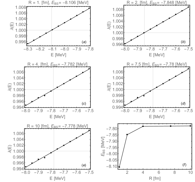
Figure 1: $(a)$ - $(e)$: The eigenvalue $\lambda$ that is closest to $1$ as a functions of the energy $E$. The screened Coulomb potential from [7] was used and consecutive plots correspond to different screening radii used in equation (6). The crosses indicate the extrapolated bound state energies $E_{BS}$ and $\lambda=1$. $(f)$: The extrapolated bound state energy $E_{BS}$ as a function of the screening radius $R$. Calculations were perfomed during the first run (see text) and use both the 2N and 3N force.

Figure 2 shows selected scalar functions for the Faddeev component of the ³He bound state obtained during the second run. All plots contain both the $\psi$ functions from (5) (that were reconstructed using (14)) and the $\beta$ functions from (15). The obtained values of these functions practically overlap, verifying the solution. The additional $T=\frac{3}{2}$ component is visible only in the dominant, first, scalar function on plot $(a)$. In Fig. 3 selected scalar functions obtained during the first run are shown. When these two plots, $(a)$ and $(b)$, are compared with plots $(d)$ and $(e)$ from Fig. 2 numerical artifacts are visible for low values of $q$. The disappearance of these artifacts in the second run is indicative of the positive effects of the changes made in the second run of calculations. It should, however, be noted that the numerical artifacts observed in the first run affect only the non-dominant scalar functions whose values are relatively very small. For this reason they are not expected to have a significant impact on the extrapolated bound state energy and other observables.

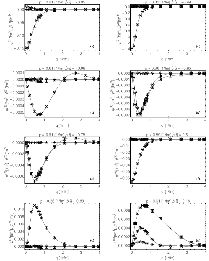
Figure 2: Selected scalar functions for the Faddeev component of the ³He bound state plotted as a function of the Jacobi momentum $\boldsymbol{q}$ magnitude. Scalar functions obtained directly using (14) are marked using solid markers while functions obtained using (15) are marked using empty markers. Squares circles and diamonds correspond to the three isospin states: $t=0,T=\frac{1}{2}$; $t=1,T=\frac{1}{2}$ and $t=1,T=\frac{3}{2}$ respectively. Calculations were performed during the second run (see text) using both 2N and 3N nuclear forces and a screened Coulomb interaction form [7] with screening radius $R=10[\text{fm}]$ (the potential goes to zero at distances greater then $3R=30[\text{fm}]$). The eigenvalue from (6) for energy $E=-7.72654[\text{MeV}]$ was $\lambda=0.99997$.

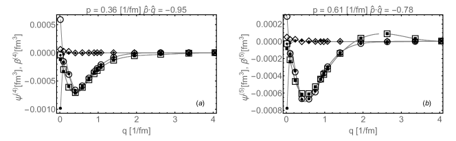
Figure 3: Similar to $(d)$, $(e)$ from Fig. 2 but the scalar functions were obtained during the first run (see text). Calculations were carried out using both 2N and 3N nuclear forces and a screened Coulomb interaction form [7] with screening radius $R=10[\text{fm}]$ (the potential goes to zero at distances greater then $3R=30[\text{fm}]$). The eigenvalue from (6) for energy $E=-7.77833[\text{MeV}]$ was $\lambda=0.99996$.

Figure 4 shows selected scalar functions $\Psi$ for the full ³He bound state obtained using (16) during the second run. All plots also contain the $\frac{1}{3}\zeta$ functions from (18). The values of these two functions essentially overlap again verifying the numerical realization. Differences appear for non-dominant scalar functions and at low values of the momenta and angles. These differences can be attributed to problems with interpolations in regions close to the function domain boundaries and are not visible in Fig. 4 where the same values of $p$ and $\hat{\boldsymbol{p}}\cdot\hat{\boldsymbol{q}}$ were used as in Fig. 2 for the purpouse of comparison. Figure 5 exemplifies the dependence of the dominant, first, scalar function $\Psi^{(1)}$ for the full ³He bound state on the magnitude of both Jacobi momenta $p,q$ for a given angle $\hat{\boldsymbol{p}}\cdot\hat{\boldsymbol{q}}$. It can be observed that the scalar function quickly drops to zero in a region where the momenta are greater then $\approx 2[\frac{1}{\text{fm}}]$.

Analogous results for ³H are shown in Figs. 6 and 7. The differences between the two dominant Faddeev component scalar functions $\psi$ are shown in Fig. 8 for ³He and ³H. The disappearance of the $T=\frac{3}{2}$ component can be clearly seen when going from ³He to ³H. In both $(a)$ and $(b)$ the $T=\frac{1}{2}$ components are dominant. This dominance is also clearly visible in Fig. 9 where $(a)$ and $(b)$ contain the largest scalar functions $\Psi$ for the full wave function of ³H and ³He.

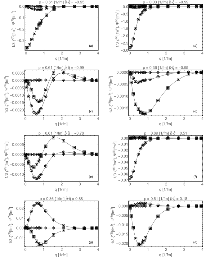
Figure 4: Selected scalar functions for the ³He bound state. Scalar functions obtained using (16) are marked using solid markers while functions obtained using (18) are marked using empty markers. Squares, circles and diamonds respectively denote the three isospin states: $t=0,T=\frac{1}{2}$; $t=1,T=\frac{1}{2}$ and $t=1,T=\frac{3}{2}$. Calculations were performed during the second run (see text) using both 2N and 3N nuclear forces and a screened Coulomb interaction form [7] with screening radius $R=10[\text{fm}]$ (the potential goes to zero at distances greater then $3R=30[\text{fm}]$). The eigenvalue from (6) for energy $E=-7.72654[\text{MeV}]$ was $\lambda=0.99997$.

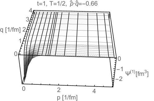
Figure 5: Dominant scalar function for the ³He bound state plotted as a function of the magnitude of the Jacobi momenta $p$, $q$ for a chosen value of $\hat{\boldsymbol{p}}\cdot\hat{\boldsymbol{q}}$.

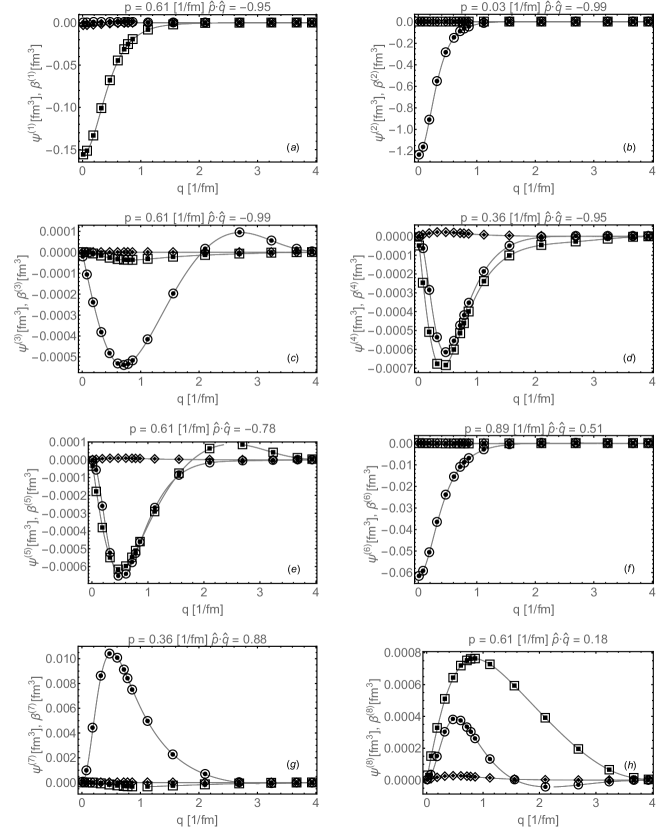
Figure 6: Same as in Fig. 2 but for ³H. The eigenvalue from (6) for energy $E=-8.4043[\text{MeV}]$ was $\lambda=0.99998$.

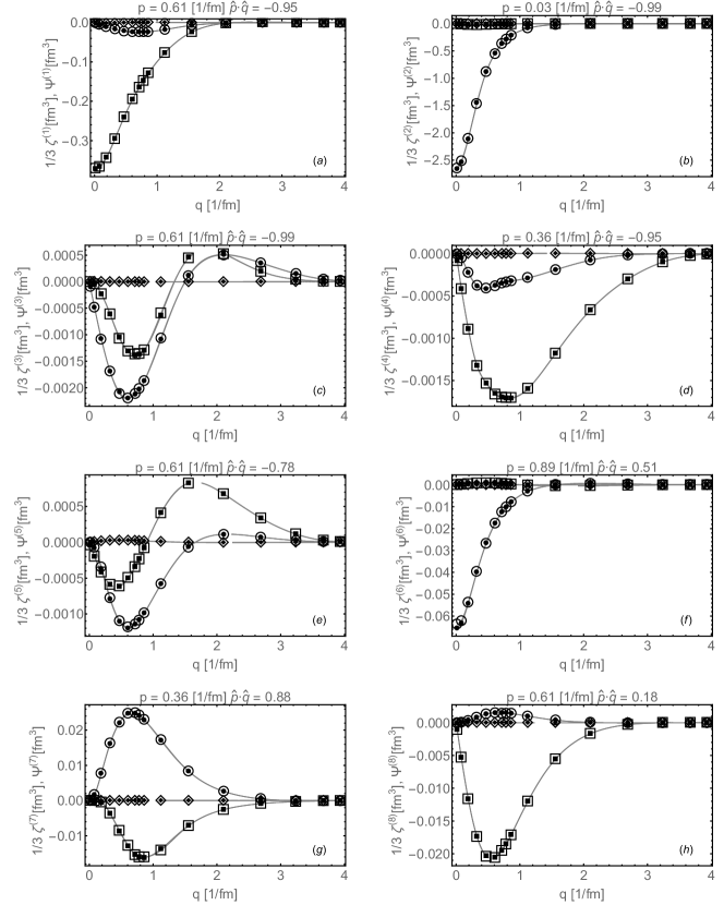
Figure 7: Same as in Fig. 4 but for ³H. The eigenvalue from (6) for energy $E=-8.4043[\text{MeV}]$ was $\lambda=0.99998$.

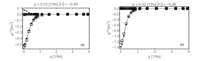
Figure 8: Similar to Figure 2 and 6. Comparison of two dominant scalar functions ($(a)$ : $\psi^{(1)}$, $(b)$ : $\psi^{(2)}$) for the Faddeev component of ³H and ³He. Squares, circles, and diamonds denote the three isospin states: $t=0,T=\frac{1}{2}$; $t=1,T=\frac{1}{2}$ and $t=1,T=\frac{3}{2}$ respectively. Empty markers correspond to ³H and solid markers correspond to ³He.

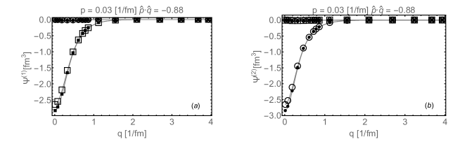
Figure 9: Similar to Figure 4 and 7. Comparison of two dominant scalar functions ($(a)$ : $\Psi^{(1)}$, $(b)$ : $\Psi^{(2)}$) for the ³H and ³He bound state. Squares, circles, and diamonds denote the three isospin states: $t=0,T=\frac{1}{2}$; $t=1,T=\frac{1}{2}$ and $t=1,T=\frac{3}{2}$ respectively. Empty markers correspond to ³H and solid markers correspond to ³He.

Tables 1 and 2 contain expectation values of the kinetic, 2N and 3N potential energies, for ³He and ³H, respectively. The sum of these expectation values is close to the extrapolated bound state energy. Differences can be attributed to the small number of grid points used to represent the scalar functions. The values in these tables were obtained using the expressions from [5]. The numerical integrals necessary to calculate the expectation values of the 3N force are very similar to the ones necessary to implement $\check{A}_{G_{0}V^{(1)}}$ in B.3. This made it possible to benefit from using the new parametrization of the integrals that is described in Appendix B.3 also when calculating the expectation value of the 3N force.

$$\begin{array}[]{ccccc}<E_{\text{kin}}>&<E_{\text{pot}}^{2N}>&<E_{\text{C}}^{2N}>&<E_{\text{pot}}^{3N}>&\Sigma\\ 32.36&-39.91&0.6929&-0.774&-7.628\\ \end{array}$$

Table 1: Expectation values (in $[\text{MeV}]$) for the kinetic energy ($E_{\text{kin}}$), the strong 2N potential ($E_{\text{pot}}^{2N}$), the screened Coulomb interaction ($E_{\text{C}}^{2N}$), and the 3N force ($E_{\text{pot}}^{3N}$). These values were obtained using the methods outlined in [5] from ³He bound state scalar functions obtained during the second run (see text). The bound state was calculated using both 2N and 3N forces. The eigenvalue from (6) for energy $E=-7.72654[\text{MeV}]$ was $\lambda=0.99997$.

$$\begin{array}[]{cccc}<E_{\text{kin}}>&<E_{\text{pot}}^{2N}>&<E_{\text{pot}}^{3N}>&\Sigma\\ 32.91&-40.45&-0.7848&-8.329\\ \end{array}$$

Table 2: Expectation values (in $[\text{MeV}]$) for the kinetic energy ($E_{\text{kin}}$), the strong 2N potential ($E_{\text{pot}}^{2N}$), and the 3N force ($E_{\text{pot}}^{3N}$). These values were obtained using the methods outlined in [5] from ³H bound state scalar functions obtained during the second run (see text). The bound state was calculated using both 2N and 3N forces. The eigenvalue from (6) for energy $E=-8.4043[\text{MeV}]$ was $\lambda=0.99998$. Additionally, the expectation value of the 2N screened Coulomb interaction was calculated: $0.7054[\text{MeV}]$.

Tables 3 and 4 contain expectation values for ³He and ³H calculated during the second run and without using a 3N force. Similarly as in Tab. 1 and 2 the sum of the expectation values is close to the extrapolated bound state energy and the difference can be attributed to the small number of grid points used to represent scalar functions. Additionally, the expectation values of the 3N potential were calculated for ³He and ³H (obtained without using a 3N force). These values are relatively small and given in the captions of Tab. 3 and 4. Finally in Fig. 10 two dominant scalar functions $\Psi$ for the ³He bound state calculated with a 3N force and without a 3N force are compared. The largest differences appear for the $T=\frac{1}{2}$ components.

$$\begin{array}[]{cccc}<E_{\text{kin}}>&<E_{\text{pot}}^{2N}>&<E_{C}^{2N}>&\Sigma\\ 30.73&-38.7&0.6953&-7.268\\ \end{array}$$

Table 3: Expectation values (in $[\text{MeV}]$) for the kinetic energy ($E_{\text{kin}}$), the strong 2N potential ($E_{\text{pot}}^{2N}$), and the 3N force ($E_{\text{pot}}^{3N}$). These values were obtained using the methods outlined in [5] from ³He bound state scalar functions obtained during the second run (see text). The bound state was calculated using only 2N forces. The eigenvalue from (6) for energy $E=-7.34124[\text{MeV}]$ was $\lambda=0.99997$. Additionally, the expectation value of the 3N force was calculated: $0.03634[\text{MeV}]$.

$$\begin{array}[]{ccc}<E_{\text{kin}}>&<E_{\text{pot}}^{2N}>&\Sigma\\ 31.32&-39.29&-7.973\\ \end{array}$$

Table 4: Expectation values (in $[\text{MeV}]$) for the kinetic energy ($E_{\text{kin}}$), the strong 2N potential ($E_{\text{pot}}^{2N}$), and the 3N force ($E_{\text{pot}}^{3N}$). These values were obtained using the methods outlined in [5] from ³H bound state scalar functions obtained during the second run (see text). The bound state was calculated using only 2N forces. The eigenvalue from (6) for energy $E=-8.02347[\text{MeV}]$ was $\lambda=0.99997$. Additionally, the expectation value of the screened Coulomb interaction: $0.7096[\text{MeV}]$ and 3N force: $0.0578[\text{MeV}]$ was calculated.

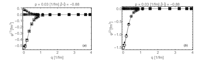
Figure 10: Similar to Figure 2 and 6. Comparison of two dominant scalar functions for the ³He Faddeev component calculated with and without the 3N force. Squares circles and diamonds respectively denote the three isospin states: $t=0,T=\frac{1}{2}$; $t=1,T=\frac{1}{2}$ and $t=1,T=\frac{3}{2}$. Empty markers correspond to ³He calculated without the 3NF and solid markers correspond to ³He calculated with the 3N force. In calculations without the 3N force the eigenvalue from (6) for energy $E=-7.34124[\text{MeV}]$ was $\lambda=0.99997$.

The obtained ³H and ³He wave functions were the starting point used to calculate matrix elements necessary to describe triton beta decay were calculated for two simple single nucleon current models. Details of this calculation are available in Appendix C. Numerical values for the matrix elements of the Fermi current for particle one:

$$\langle\boldsymbol{k}^{\prime}_{1}\mid\check{\rho}_{F}(1)\mid\boldsymbol{k}_{1}\rangle=\check{\tau}(1)_{+}\,\check{1}$$ (19)

where $\boldsymbol{k^{\prime}_{1}}$, $\boldsymbol{k}$ are the momenta of particle one in the final and initial states, $\check{\tau}(1)_{+}$ is the isospin raising operator and $\check{1}$ is the identity operator in the spin space of particle one, are gathered in Tab. 5.

Matrix elements for the $z$ component of the Gamow-Teller current:

$$\langle\boldsymbol{k}^{\prime}_{1}\mid\check{\boldsymbol{j}}_{GTz}(1)\mid\boldsymbol{k}_{1}\rangle=\check{\tau}(1)_{+}\,\check{\sigma}(1)_{z},$$ (20)

where $\check{\sigma}(1)_{z}$ is a component of the vector spin operator $\check{\boldsymbol{\sigma}}(1)=(\check{\sigma}(1)_{x},\check{\sigma}(1)_{y},\check{\sigma}(1)_{z})$, are gathered in Tab. 6. In order to verify these results several additional calculations were performed. First, matrix elements of (20) were calculated with $\check{\sigma}(1)_{z}$ replaced by the spherical components of the spin $\check{\sigma}(1)_{+1}$, $\check{\sigma}(1)_{-1}$:

$$\check{j}_{GT+}(1)=\check{\tau}(1)_{+}\check{\sigma}(1)_{+1},$$ (21)

$$\check{j}_{GT-}(1)=\check{\tau}(1)_{+}\check{\sigma}(1)_{-1}.$$ (22)

These results are gathered in Tab. 7. Since observables are proportional to the sum over the spin projections in the initial and final states $m_{i}$, $m_{f}$:

$$S(\check{j})=\sum_{m_{f}=\pm\frac{1}{2}}\sum_{m_{i}=\pm\frac{1}{2}}|\langle^{3}\text{He}\,\,m_{f}\mid\check{j}(1)\mid^{3}\text{H}\,\,m_{i}\rangle|^{2}$$ (23)

this sum was calculated for $\check{\sigma}(1)_{z}$, $\check{\sigma}(1)_{+1}$ and $\check{\sigma}(1)_{-1}$ and compared in Tab. 8. The values are essentialy the same and this confirmes the corectness of the calculations form Tab. 6 and 7. Next, the expectation values of the $\frac{1}{2}\left(\check{1}+\check{\tau}(1)_{3}\right)$ isospin operator ($\check{\tau}(1)_{3}$ is the third component of the ispspin for particle $1$) were calculated. The obtained values were $0.666395$ for ³He and $0.333533$ for ³H. These two results provide an additional verification since they are very close to $\frac{2}{3}$ and $\frac{1}{3}$ that could be expected for ³He and ³H respectively. Results for simple single nucleon currents that are presented here, open up the possibility to perform calculations with more complicated models and two - nucleon currents.

$$\begin{array}[]{c|c}\text{matrix element:}&\text{value:}\\ \hline\cr\langle^{3}\text{He}\,\,m_{f}=-\frac{1}{2}\mid\check{\rho}_{F}(1)\mid^{3}\text{H}\,\,m_{i}=-\frac{1}{2}\rangle&0.332825\\ \langle^{3}\text{He}\,\,m_{f}=\frac{1}{2}\mid\check{\rho}_{F}(1)\mid^{3}\text{H}\,\,m_{i}=\frac{1}{2}\rangle&0.332825\\ \end{array}$$

Table 5: Non zero matrix elements of the Fermi current for particle $1$. The spin projection of the triton in the initial state is $m_{i}$ and the spin projection of helium-$3$ in the final state is $m_{f}$.

$$\begin{array}[]{c|c}\text{matrix element:}&\text{value:}\\ \hline\cr\langle^{3}\text{He}\,\,m_{f}=-\frac{1}{2}\mid\check{j}_{GTz}(1)\mid^{3}\text{H}\,\,m_{i}=-\frac{1}{2}\rangle&0.310749\\ \langle^{3}\text{He}\,\,m_{f}=\frac{1}{2}\mid\check{j}_{GTz}(1)\mid^{3}\text{H}\,\,m_{i}=\frac{1}{2}\rangle&-0.310749\\ \end{array}$$

Table 6: Non zero matrix elements of the Gamow-Teller current for particle $1$. The spin projection of the triton in the initial state is $m_{i}$ and the spin projection of helium-$3$ in the final state is $m_{f}$.

$$\begin{array}[]{c|c}\text{matrix element:}&\text{value:}\\ \hline\cr\langle^{3}\text{He}\,\,m_{f}=\frac{1}{2}\mid\check{j}_{GT+}(1)\mid^{3}\text{H}\,\,m_{i}=-\frac{1}{2}\rangle&0.439465\\ \langle^{3}\text{He}\,\,m_{f}=-\frac{1}{2}\mid\check{j}_{GT-}(1)\mid^{3}\text{H}\,\,m_{i}=\frac{1}{2}\rangle&-0.439465\\ \end{array}$$

Table 7: Non zero matrix elements of the currents from (21) and (22). The spin projection of the triton in the initial state is $m_{i}$ and the spin projection of helium-$3$ in the final state is $m_{f}$.

$$\begin{array}[]{c|c}\text{sum:}&\text{value:}\\ \hline\cr S(\check{j}_{GTz})&0.19313\\ S(\check{j}_{GT+})&0.19313\\ S(\check{j}_{GT-})&0.19313\\ \end{array}$$

Table 8: Values of the sum from (23) for currents (20), (21) and (22). The values are essentialy the same for all cases. Since observables are proportional to (23) (among other things, the proportionality coefficients contain a factor of $3^{2}=9$ steming from the necesity to use $\check{j}(1)+\check{j}(2)+\check{j}(3)$) this verifies the calculation in Tab. 6 and 7.

4 Summary and outlook

This paper shows that three-nucleon bound state calculations with screened Coulomb potentials are possible using the “three dimensional” approach. Instead of relying on the partial wave decomposition of operators relevant to the calculation, the new approach uses the three dimensional, momentum, degrees of freedom of the nucleons directly. A practical numerical realization of these calculations is made feasible by the idea to write the three-nucleon state as a linear combination of spin operators and scalar functions. These scalar functions effectively define the state and are the central object in the “three dimensional” calculations.

The dependency of the bound state energy on the screening radius of the Coulomb interaction was shown and it was determined that it is sufficient to perform calculations with a screening radius of $10[\text{fm}]$ (for the model of Coulomb interaction used this means that the potential goes to zero at distances larger then $30[\text{fm}]$). At this value the values of observables are expected to be converged. Plots showing selected scalar functions were given. Apart from the scalar functions that define the bound state, the plots also contain additional, overlapping, functions that verify the validity of the obtained solution.

Having calculated the bound states of ³He and ³H, the expectation values of the kinetic and potential energies were calculated. This further confirmed the corectness of the obtained results but also showed that it would be beneficial to perform the calculations using a grater number of grid points to represent the scalar functions. Calculations with an increased number of points are planned for more modern models of chiral two- and three- nucleon interactions.

Additionally, basic matrix elements related to the triton beta decay were calculated. These matrix elements are based on simple models of nuclear currents and can be directly used to calculate observables related to that decay.

Appendix A Spin operators in 3N operator form

Below is a list of spin operators used in the operator form of the 3N (Faddeev, bound) state (1). Spin operators acting in the spaces of particle $1$, $2$, $3$ are denoted as $\check{\boldsymbol{\sigma}}(1)$, $\check{\boldsymbol{\sigma}}(2)$, $\check{\boldsymbol{\sigma}}(3)$ respectively and $\check{\boldsymbol{\sigma}}(2,3)=\frac{1}{2}(\check{\boldsymbol{\sigma}}(2)-\check{\boldsymbol{\sigma}}(3))$. Vectors $\boldsymbol{p}$, $\boldsymbol{q}$ are the Jacobi momenta of the 3N system (if $\boldsymbol{k}_{1,2,3}$ are individual particle momenta then $\boldsymbol{p}=\frac{1}{2}(\boldsymbol{k}_{2}-\boldsymbol{k}_{3})$, $\boldsymbol{q}=\frac{2}{3}(\boldsymbol{k}_{1}-\frac{1}{2}(\boldsymbol{k}_{2}+\boldsymbol{k}_{3}))$).

$$\check{O}_{1}(\boldsymbol{p},\boldsymbol{q}) =\check{1},$$

$$\check{O}_{2}(\boldsymbol{p},\boldsymbol{q}) =\frac{1}{\sqrt{3}}\check{\boldsymbol{\sigma}}(2,3)\cdot\check{\boldsymbol{\sigma}}(1),$$

$$\check{O}_{3}(\boldsymbol{p},\boldsymbol{q}) =\sqrt{\frac{3}{2}}\frac{1}{i}\check{\boldsymbol{\sigma}}(1)\cdot(\hat{\boldsymbol{p}}\times\hat{\boldsymbol{q}}),$$

$$\check{O}_{4}(\boldsymbol{p},\boldsymbol{q}) =\frac{1}{\sqrt{2}}\left(i\check{\boldsymbol{\sigma}}(2,3)\cdot(\hat{\boldsymbol{p}}\times\hat{\boldsymbol{q}})-\right.$$

$$\left.(\check{\boldsymbol{\sigma}}(1)\times\check{\boldsymbol{\sigma}}(2,3))\cdot(\hat{\boldsymbol{p}}\times\hat{\boldsymbol{q}})\right),$$

$$\check{O}_{5}(\boldsymbol{p},\boldsymbol{q}) =\frac{1}{i}\left(\check{\boldsymbol{\sigma}}(2,3)\cdot(\hat{\boldsymbol{p}}\times\hat{\boldsymbol{q}})-\right.$$

$$\left.\frac{i}{2}(\check{\boldsymbol{\sigma}}(1)\times\check{\boldsymbol{\sigma}}(2,3))\cdot(\hat{\boldsymbol{p}}\times\hat{\boldsymbol{q}})\right),$$

$$\check{O}_{6}(\boldsymbol{p},\boldsymbol{q}) =\sqrt{\frac{3}{2}}\left(\check{\boldsymbol{\sigma}}(2,3)\cdot\hat{\boldsymbol{p}}\boldsymbol{\check{\sigma}}(1)\cdot\hat{\boldsymbol{p}}-\frac{1}{3}\boldsymbol{\check{\sigma}}(2,3)\cdot\boldsymbol{\check{\sigma}}(1)\right),$$

$$\check{O}_{7}(\boldsymbol{p},\boldsymbol{q}) =\sqrt{\frac{3}{2}}\left(\check{\boldsymbol{\sigma}}(2,3)\cdot\hat{\boldsymbol{q}}\boldsymbol{\check{\sigma}}(1)\cdot\hat{\boldsymbol{q}}-\frac{1}{3}\boldsymbol{\check{\sigma}}(2,3)\cdot\boldsymbol{\check{\sigma}}(1)\right),$$

$$\check{O}_{8}(\boldsymbol{p},\boldsymbol{q}) =\frac{3}{2}\frac{1}{\sqrt{5}}\left(\check{\boldsymbol{\sigma}}(2,3)\cdot\hat{\boldsymbol{q}}\boldsymbol{\check{\sigma}}(1)\cdot\hat{\boldsymbol{p}}+\right.$$

$$\left.\boldsymbol{\check{\sigma}}(2,3)\cdot\boldsymbol{\check{p}}\check{\boldsymbol{\sigma}}(1)\cdot\hat{\boldsymbol{q}}-\frac{2}{3}\hat{\boldsymbol{p}}\cdot\hat{\boldsymbol{q}}\boldsymbol{\check{\sigma}}(2,3)\cdot\check{\boldsymbol{\sigma}}(1)\right),$$

Appendix B Explicit form of operators acting on scalar functions

B.1 Permutation operator

The treatment of the permutation operator in the calculations is similar to the approach that was used in [5]. The differences are only formal and related to a slightly different bookkeeping. For this reason only a sketch of the derivations is provided here. More details are available in Chapter $10$ of [12].

Firstly, the operator form from for the states $\mid\alpha\rangle$, $\mid\gamma\rangle$ from (1) is inserted into both sides of:

$$\left(\check{1}+\check{P}\right)\mid\alpha\rangle=\mid\gamma\rangle.$$

Next the spin dependency is removed from this equation by projecting it from the left onto different spin states $\langle\chi^{m}\mid\check{O}_{k}(\boldsymbol{p}^{\prime}\boldsymbol{q}^{\prime})$ for $k=1\ldots 8$ and summing over $m$. Finally the resulting integral equations are transformed in to give the expression for the scalar functions that define $\gamma$.

Unlike [5] the action of the permutation on the combined isospin - spin state of the 3N system is considered. Instead of using the $F_{tt^{\prime}T}$ coefficients from [5] the following functions are introduced:

$$F^{\text{id}}_{t^{\prime}T^{\prime}k;tTi}(\boldsymbol{p}^{\prime},\boldsymbol{q^{\prime}})=$$

$$\sum_{m}{\langle\left(t^{\prime}\frac{1}{2}\right)T^{\prime}M_{T^{\prime}}\mid\otimes\langle\chi^{m}\mid}\left[\check{1}\otimes\check{O}_{k}(\boldsymbol{p}^{\prime},\boldsymbol{q}^{\prime})\right]$$

$$\left[\check{1}\otimes\check{O}_{i}(\boldsymbol{p}^{\prime},\boldsymbol{q}^{\prime})\right]{\mid\left(t\frac{1}{2}\right)TM_{T}\rangle\otimes\mid\chi^{m}\rangle},$$ (24)

$$F_{t^{\prime}T^{\prime}k;tTi}^{1223}(\boldsymbol{p}^{\prime},\boldsymbol{q^{\prime}})=$$

$$\sum_{m}{\langle\left(t^{\prime}\frac{1}{2}\right)T^{\prime}M_{T^{\prime}}\mid\otimes\langle\chi^{m}\mid}$$

$$\left[\check{1}\otimes\check{O}_{k}(\boldsymbol{p}^{\prime},\boldsymbol{q}^{\prime})\right]\left[\check{P}_{12}\right]\left[\check{P}_{23}\right]$$

$$\left[\check{1}\otimes\check{O}_{i}(\boldsymbol{P}^{2312}(\boldsymbol{p}^{\prime},\boldsymbol{q}^{\prime}),\boldsymbol{Q}^{2312}(\boldsymbol{p}^{\prime},\boldsymbol{q}^{\prime}))\right]$$

$${\mid\left(t\frac{1}{2}\right)TM_{T}\rangle\otimes\mid\chi^{m}\rangle},$$ (25)

$$F_{t^{\prime}T^{\prime}k;tTi}^{1323}(\boldsymbol{p}^{\prime},\boldsymbol{q^{\prime}})=$$

$$\sum_{m}{\langle\left(t^{\prime}\frac{1}{2}\right)T^{\prime}M_{T^{\prime}}\mid\otimes\langle\chi^{m}\mid}$$

$$\left[\check{1}\otimes\check{O}_{k}(\boldsymbol{p}^{\prime},\boldsymbol{q}^{\prime})\right]\left[\check{P}_{13}\right]\left[\check{P}_{23}\right]$$

$$\left[\check{1}\otimes\check{O}_{i}(\boldsymbol{P}^{2313}(\boldsymbol{p}^{\prime},\boldsymbol{q}^{\prime}),\boldsymbol{Q}^{2313}(\boldsymbol{p}^{\prime},\boldsymbol{q}^{\prime}))\right]$$

$${\mid\left(t\frac{1}{2}\right)TM_{T}\rangle\otimes\mid\chi^{m}\rangle},$$ (26)

where $\left[\check{P}_{ij}\right]$ are the matrix representations of the operator exchanging particles $i$ and $j$ in the combined isospin - spin space of the 3N system. The functions $\boldsymbol{P}^{2313}$, $\boldsymbol{P}^{2312}$, $\boldsymbol{Q}^{2313}$, and $\boldsymbol{Q}^{2312}$ are a direct result of applying the permutation operator to Jacobi momentum eignestates:

$$\check{P}_{23}\check{P}_{12}\mid\boldsymbol{p}^{\prime}\boldsymbol{q}^{\prime}\rangle=\mid\boldsymbol{P}^{2312}(\boldsymbol{p}^{\prime},\boldsymbol{q}^{\prime})\boldsymbol{Q}^{2312}(\boldsymbol{p}^{\prime},\boldsymbol{q}^{\prime})\rangle,$$

$$\boldsymbol{P}^{2312}(\boldsymbol{p}^{\prime},\boldsymbol{q}^{\prime})=-\frac{1}{4}(2\boldsymbol{p}^{\prime}+3\boldsymbol{q}^{\prime}),$$

$$\boldsymbol{Q}^{2312}(\boldsymbol{p}^{\prime},\boldsymbol{q}^{\prime})=\boldsymbol{p}^{\prime}-\frac{1}{2}\boldsymbol{q}^{\prime},$$

$$\check{P}_{23}\check{P}_{13}\mid\boldsymbol{p}^{\prime}\boldsymbol{q}^{\prime}\rangle=\mid\boldsymbol{P}^{2313}(\boldsymbol{p}^{\prime},\boldsymbol{q}^{\prime})\boldsymbol{Q}^{2313}(\boldsymbol{p}^{\prime},\boldsymbol{q}^{\prime})\rangle$$

$$\boldsymbol{P}^{2313}(\boldsymbol{p}^{\prime},\boldsymbol{q}^{\prime})=-\frac{1}{4}(2\boldsymbol{p}^{\prime}-3\boldsymbol{q}^{\prime})$$

$$\boldsymbol{Q}^{2313}(\boldsymbol{p}^{\prime},\boldsymbol{q}^{\prime})=-\boldsymbol{p}^{\prime}-\frac{1}{2}\boldsymbol{q}^{\prime}.$$

If the first part of the permutation operator $\check{P}=\check{P}_{12}\check{P}_{23}+\check{P}_{13}\check{P}_{23}$, namely $\check{P}_{12}\check{P}_{23}$, is applied to a 3N state $\mid\alpha\rangle$ written in the form of equation (1) ($\mid\alpha\rangle$ is defined by a set of scalar functions $\alpha$) then this results in a new 3N state $\mid\gamma\rangle$ that can also be written in the form from equation (1) ($\mid\gamma\rangle$ is defined by a set of scalar functions $\gamma$). This introduces the operator $\check{P}^{\mathrm{scalar}}_{1223}$ that is defined via the relation:

$$\left(\check{P}^{\mathrm{scalar}}_{1223}\alpha\right)_{t^{\prime}T^{\prime}}^{(k)}(|\boldsymbol{p}^{\prime}|,|\boldsymbol{q}^{\prime}|,\hat{\boldsymbol{p}}^{\prime}\cdot\hat{\boldsymbol{q}}^{\prime})=$$

$$\gamma_{t^{\prime}T^{\prime}}^{(k)}(|\boldsymbol{p}^{\prime}|,|\boldsymbol{q}^{\prime}|,\hat{\boldsymbol{p}}^{\prime}\cdot\hat{\boldsymbol{q}}^{\prime})$$ (27)

or more precisely:

$$\gamma_{t^{\prime}T^{\prime}}^{(k)}(|\boldsymbol{p}^{\prime}|,|\boldsymbol{q}^{\prime}|,\hat{\boldsymbol{p}}^{\prime}\cdot\hat{\boldsymbol{q}}^{\prime})=$$

$$\sum_{tT}\sum_{i=1}^{8}\phi_{tT}^{(i)}(|\boldsymbol{P}^{2312}(\boldsymbol{p}^{\prime},\boldsymbol{q}^{\prime})|,|\boldsymbol{Q}^{2312}(\boldsymbol{p}^{\prime},\boldsymbol{q}^{\prime})|,$$

$$\hat{\boldsymbol{P}}^{2312}(\boldsymbol{p}^{\prime},\boldsymbol{q}^{\prime})\cdot\hat{\boldsymbol{Q}}^{2312}(\boldsymbol{p}^{\prime},\boldsymbol{q}^{\prime}))$$

$$C_{t^{\prime}T^{\prime}k;tTi}^{1223}(\boldsymbol{p}^{\prime},\boldsymbol{q^{\prime}}),$$ (28)

where the functions $C_{t^{\prime}T^{\prime}k;tTi}^{1223}$ are:

$$C_{t^{\prime}T^{\prime}k;tTi}^{1223}(\boldsymbol{p}^{\prime},\boldsymbol{q^{\prime}})=$$

$$\sum_{t^{\prime\prime}T^{\prime\prime}j}(F^{\text{id}})^{-1}_{t^{\prime}T^{\prime}k;t^{\prime\prime}T^{\prime\prime}j}(\boldsymbol{p}^{\prime},\boldsymbol{q^{\prime}})F^{1223}_{t^{\prime\prime}T^{\prime\prime}j;tTi}(\boldsymbol{p}^{\prime},\boldsymbol{q^{\prime}})$$ (29)

and

$$\sum_{t^{\prime\prime}T^{\prime\prime}j}(F^{\text{id}})^{-1}_{t^{\prime}T^{\prime}k;t^{\prime\prime}T^{\prime\prime}j}(\boldsymbol{p}^{\prime},\boldsymbol{q^{\prime}})F^{\text{id}}_{t^{\prime\prime}T^{\prime\prime}j;tTi}(\boldsymbol{p}^{\prime},\boldsymbol{q^{\prime}})=$$

$$\delta_{t^{\prime}t}\delta_{T^{\prime}T}\delta_{ki}.$$ (30)

The second part of the permutation operator $\check{P}_{13}\check{P}_{23}$ can be introduced in a completely analogous way by replacing everywhere in (27) - (30) $1223$ by $1323$:

$$\left(\check{P}^{\mathrm{scalar}}_{1323}\alpha\right)_{t^{\prime}T^{\prime}}^{(k)}(|\boldsymbol{p}^{\prime}|,|\boldsymbol{q}^{\prime}|,\hat{\boldsymbol{p}}^{\prime}\cdot\hat{\boldsymbol{q}}^{\prime})=$$

$$\gamma_{t^{\prime}T^{\prime}}^{(k)}(|\boldsymbol{p}^{\prime}|,|\boldsymbol{q}^{\prime}|,\hat{\boldsymbol{p}}^{\prime}\cdot\hat{\boldsymbol{q}}^{\prime}).$$ (31)

Finally, the $\check{1}$ in $\check{1}+\check{P}$ is just the identity operator and does not change the scalar function. In the end:

$$\left(\check{A}_{\text{1 + P}}\,\,\alpha\right)_{t^{\prime}T^{\prime}}^{(k)}(|\boldsymbol{p}^{\prime}|,|\boldsymbol{q}^{\prime}|,\hat{\boldsymbol{p}}^{\prime}\cdot\hat{\boldsymbol{q}}^{\prime})=$$

$$\alpha_{t^{\prime}T^{\prime}}^{(k)}(|\boldsymbol{p}^{\prime}|,|\boldsymbol{q}^{\prime}|,\hat{\boldsymbol{p}}^{\prime}\cdot\hat{\boldsymbol{q}}^{\prime})+$$

$$\left(\check{P}^{\mathrm{scalar}}_{1223}\alpha\right)_{t^{\prime}T^{\prime}}^{(k)}(|\boldsymbol{p}^{\prime}|,|\boldsymbol{q}^{\prime}|,\hat{\boldsymbol{p}}^{\prime}\cdot\hat{\boldsymbol{q}}^{\prime})+$$

$$\left(\check{P}^{\mathrm{scalar}}_{1323}\alpha\right)_{t^{\prime}T^{\prime}}^{(k)}(|\boldsymbol{p}^{\prime}|,|\boldsymbol{q}^{\prime}|,\hat{\boldsymbol{p}}^{\prime}\cdot\hat{\boldsymbol{q}}^{\prime}).$$ (32)

A more detailed derivation of these expressions is available in Chapter $10$ of [12]. The numerical implementation of $\check{P}^{\mathrm{scalar}}_{1223}$ and $\check{P}^{\mathrm{scalar}}_{1323}$ requires the use of interpolations, the calculations presented in this paper use cubic Hermitian splines.

B.2 2N potential

This section contains expressions necessary to implement the action of the 2N potential on the scalar functions from the operator form (1). Since the approach used in this section is very similar to the methods presented in [5], below only a sketch of the deriviations is presented.

It is well established (see eg. [9]) that the matrix element of the 2N force between 3N Jacobi momentum eigenstates $\langle\boldsymbol{p}^{\prime}\boldsymbol{q}^{\prime}\mid$, $\mid\boldsymbol{p}\boldsymbol{q}\rangle$ can be written as:

$$\langle\boldsymbol{p}^{\prime}\boldsymbol{q}^{\prime}\mid\check{V}\mid\boldsymbol{p}\boldsymbol{q}\rangle=\delta^{3}(\boldsymbol{q}^{\prime}-\boldsymbol{q})$$

$$\sum_{i=1}^{6}\sum_{t^{\prime}T^{\prime}}\sum_{tT}\delta_{tt^{\prime}}\delta_{M_{T^{\prime}}M_{T}}v^{t^{\prime}T^{\prime}tT}_{i}(p^{\prime},p,\hat{\boldsymbol{p}}^{\prime}\cdot\hat{\boldsymbol{p}})$$

$$(\check{1}\otimes\check{w}_{i}(\boldsymbol{p}^{\prime},\boldsymbol{p}))\mid(t^{\prime}\frac{1}{2})T^{\prime}M_{T^{\prime}}\rangle\langle(t\frac{1}{2})TM_{T}\mid$$ (33)

where $\check{1}\otimes\check{w}_{i}(p^{\prime},p,\hat{\boldsymbol{p}}^{\prime}\cdot\hat{\boldsymbol{p}})$ is a spin operator with $\check{w}_{i}(p^{\prime},p,\hat{\boldsymbol{p}}^{\prime}\cdot\hat{\boldsymbol{p}})$ acting in the space of particles $2$ and $3$. Any operator that can be written using (33) implicitly satisfies symmetries with respect to spatial rotations, parity inversion, time reversal and particle exchange and is effectively defined by the set of scalar functions of the relative final and initial momenta $v^{t^{\prime}T^{\prime}tT}_{i}(p^{\prime},p,\hat{\boldsymbol{p}}^{\prime}\cdot\hat{\boldsymbol{p}})$. The spin operators $\check{w}_{i}(\boldsymbol{p}^{\prime},\boldsymbol{p})$ from (33) are [8, 9]:

$$\check{w}_{1}(\boldsymbol{p}^{\prime},\boldsymbol{p})=\check{1}$$

$$\check{w}_{2}(\boldsymbol{p}^{\prime},\boldsymbol{p})=\check{\boldsymbol{\sigma}}(1)\cdot\check{\boldsymbol{\sigma}}(2)$$

$$\check{w}_{3}(\boldsymbol{p}^{\prime},\boldsymbol{p})=-i(\check{\boldsymbol{\sigma}}(1)+\check{\boldsymbol{\sigma}}(2))\cdot(\boldsymbol{p}^{\prime}\times\boldsymbol{p})$$

$$\check{w}_{4}(\boldsymbol{p}^{\prime},\boldsymbol{p})=\check{\boldsymbol{\sigma}}(2)\cdot(\boldsymbol{p}^{\prime}\times\boldsymbol{p})\check{\boldsymbol{\sigma}}(3)\cdot(\boldsymbol{p}^{\prime}\times\boldsymbol{p})$$

$$\check{w}_{5}(\boldsymbol{p}^{\prime},\boldsymbol{p})=\check{\boldsymbol{\sigma}}(2)\cdot(\boldsymbol{p}^{\prime}+\boldsymbol{p})\check{\boldsymbol{\sigma}}(3)\cdot(\boldsymbol{p}^{\prime}+\boldsymbol{p})$$

$$\check{w}_{6}(\boldsymbol{p}^{\prime},\boldsymbol{p})=\check{\boldsymbol{\sigma}}(2)\cdot(\boldsymbol{p}^{\prime}\times\boldsymbol{p})\check{\boldsymbol{\sigma}}(3)\cdot(\boldsymbol{p}^{\prime}-\boldsymbol{p})$$

and are constructed from the relative momentum vector operators $\boldsymbol{p}^{\prime}$, $\boldsymbol{p}$ and the spin vector operators $\check{\boldsymbol{\sigma}}(i)$ acting in the space of particles $i=1,2$.

In the previous paper [5] the operator form (33) was used to work out the numerical implementation of $\check{G}_{0}(E)\check{V}$ in “three dimensional” bound state calculations. This was achieved by plugging the operator form (1) of 3N states $\mid\alpha\rangle$, $\mid\gamma\rangle$, the 2N potential (33) and the momentum space expression for the free propagator:

$$\langle\boldsymbol{p}^{\prime}\boldsymbol{q}^{\prime}\mid\check{G}_{0}(E)\mid\boldsymbol{p}\boldsymbol{q}\rangle=\delta^{3}(\boldsymbol{p}-\boldsymbol{p}^{\prime})\delta^{3}(\boldsymbol{q}-\boldsymbol{q}^{\prime})$$

$$\frac{1}{E-\frac{3}{4m}p^{2}-\frac{1}{2m}q^{2}}$$ (34)

into

$$\check{G}_{0}(E)\check{V}\mid\alpha\rangle=\mid\gamma\rangle,$$

and projecting the resulting equation onto a Jacobi momentum eigenstate $\langle\boldsymbol{p}^{\prime}\boldsymbol{q}^{\prime}\mid$. The spin dependency of the resulting equation was removed by projecting it from the left onto different spin states $\langle\chi^{m}\mid\check{O}_{k}(\boldsymbol{p}^{\prime}\boldsymbol{q}^{\prime})$ for $k=1\ldots 8$ and summing over $m$. The result of these manipulations is a linear relation:

$$\check{A}_{G_{0}V}(E)\alpha\equiv\gamma.$$ (35)

that defines the energy $E$ dependant operator $\check{A}_{G_{0}V}(E)$. It acts in the space of the set of scalar functions that define Faddeev component in (1). Applying the first part of the Faddeev equation (2), $\check{G}_{0}(E)\check{V}$, to a state $\mid\alpha\rangle$ written in the operator form (1) that is defined by a set of scalar functions $\alpha$ ($\alpha^{(k)}_{t^{\prime}T^{\prime}}(p^{\prime},q^{\prime},x^{\prime}=\hat{\boldsymbol{p}}^{\prime}\cdot\hat{\boldsymbol{q}}^{\prime})$) results in a new state $\mid\gamma\rangle$ that can be written in the same form (1) but with a different set of scalar functions $\gamma$ ($\gamma^{(k)}_{t^{\prime}T^{\prime}}(p^{\prime},q^{\prime},x^{\prime}=\hat{\boldsymbol{p}}^{\prime}\cdot\hat{\boldsymbol{q}}^{\prime})$). The full form of $\check{A}_{G_{0}V}(E)$ is:

$$\left(\check{A}_{G_{0}V}(E)\alpha\right)^{(k)}_{t^{\prime}T^{\prime}}(p^{\prime},q^{\prime},x^{\prime}=\hat{\boldsymbol{p}}^{\prime}\cdot\hat{\boldsymbol{q}}^{\prime})\equiv$$

$$\gamma^{(k)}_{t^{\prime}T^{\prime}}(p^{\prime},q^{\prime},x^{\prime})=$$

$$\int_{0}^{\infty}\text{d}pp^{2}\int_{-1}^{1}\text{d}x\sum_{T}\sum_{i=1}^{8}\frac{1}{E-\frac{3}{4m}p^{\prime 2}-\frac{1}{m}q^{\prime 2}}$$

$$\left\{\sum_{j=1}^{6}\int_{0}^{2\pi}\text{d}\phi\,v_{j}^{t^{\prime}T^{\prime}t^{\prime}T}(p^{\prime},p,\hat{\boldsymbol{p}}^{\prime}\cdot\hat{\boldsymbol{p}})\bar{L}_{kji}(\boldsymbol{p}^{\prime},\boldsymbol{q}^{\prime},\boldsymbol{p})\right\}$$

$$\alpha^{(i)}_{t^{\prime}T}(p,q^{\prime},x),$$ (36)

where the integral over the vector $\boldsymbol{p}$ is parametrized as:

$$\boldsymbol{p}=p(\sqrt{1-x^{2}}\cos{\phi},\sqrt{1-x^{2}}\sin{\phi},x)$$

with $p$ being the magnitude of $\boldsymbol{p}$, $\phi$ being the azimutal angle and $x$ being the cosine of the polar angle. Additionally, using the scalar character of the equations, in (36):

$$\boldsymbol{p}^{\prime}=p^{\prime}(\sqrt{1-x^{\prime 2}},0,x^{\prime}),$$

$$\boldsymbol{q}^{\prime}=q^{\prime}(0,0,1)$$

can be chosen.

The curly brackets in (36) contain integrals

$$I^{\text{2N}}_{t^{\prime}T^{\prime}T;k;i}(p^{\prime},q^{\prime},x^{\prime},p,x)=$$

$$\sum_{j=1}^{6}\int_{0}^{2\pi}\text{d}\phi\,v_{j}^{t^{\prime}T^{\prime}t^{\prime}T}(p^{\prime},p,\hat{\boldsymbol{p}}^{\prime}\cdot\hat{\boldsymbol{p}})\bar{L}_{kji}(\boldsymbol{p}^{\prime},\boldsymbol{q}^{\prime},\boldsymbol{p})$$ (37)

that can be performed once and reused later when applying $\check{G}_{0}\check{V}$ to different states (which are defined by different scalar functions $\alpha$). The $\bar{L}$ functions are defined as:

$$\bar{L}_{kji}\equiv\sum_{l}C^{-1}_{kl}L_{lji}$$

where the $C^{-1}$, $L$ coefficients are defined in equations (49), (30) from [5].

Equation (36) can be used to perform numerical calculations with both the short range and long range 2N interactions. When calculating the bound state of ³He with the screened Coulomb interaction, the operator $\check{A}_{G_{0}V}$ is further split into two parts:

$$\check{A}_{G_{0}V}=\check{A}_{G_{0}V_{NN}}+\check{A}_{G_{0}V_{C}}$$

that correspond to the short range nuclear interaction and longer ranged screened Coulomb force. The numerical implementation of both of these operators is very similar. The only practical difference is that in the long range part $\check{A}_{G_{0}V_{C}}$ the integrals $I^{\text{2N}}_{t^{\prime}T^{\prime}T;k;i}(p^{\prime},q^{\prime},x^{\prime},p,x)$ are calculated using more integration points around $p^{\prime}=p$ and $x^{\prime}=x$. Examples of grid points in the $p-x$ plane for different values of $p^{\prime}$, $x^{\prime}$ are shown in Fig. 11. Also the number of integration points along the azimuthal angle in (37) is increased, typically $256$ Gaussian points were used compared to $16$ and $64$ points for the nuclear interaction in the first and second run of the calculations.

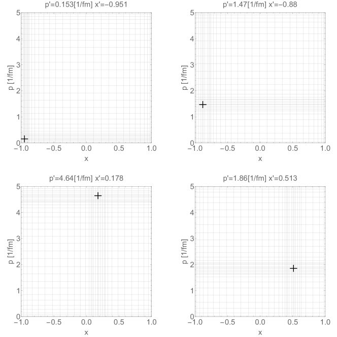
Figure 11: Integration points used for the screened Coulomb interaction in (36). Grid lines correspond to integration points in the $x$ and $p$ directions. The cross corresponds to $(x^{\prime},p^{\prime})$. Integration points in each direction are created by stiching togather several sets of Gaussian quadrature points.

For the results presented in this paper a screened Coulomb potential from Ref. [7] was used. The momentum space expressions for this interaction are given explicitly in equation (A3) and (A4) in Ref. [7]. Solutions were obtained using the same, first generation, short range NNLO 2N interaction as was used in [5] but use both the neutron-proton and proton-proton version of this interaction (the neutron-neutron interaction is approximated by the proton-proton force).

B.3 3N force

This section contains expressions necesary to implement the action of the 3N potential on the scalar functions from the operator form (1). The matrix element of the 3N force between 3N Jacobi momentum eigenstates $\langle\boldsymbol{p}^{\prime}\boldsymbol{q}^{\prime}\mid$, $\mid\boldsymbol{p}\boldsymbol{q}\rangle$ can be written [5] as:

$$\langle\boldsymbol{p}^{\prime}\boldsymbol{q}^{\prime}\mid\check{V}^{(1)}\mid\boldsymbol{p}\boldsymbol{q}\rangle=$$

$$\sum_{t^{\prime}T^{\prime}}\sum_{tT}\delta_{TT^{\prime}}\delta_{M_{T}M_{T^{\prime}}}\check{V}^{(1)}_{tt^{\prime}T}(\boldsymbol{p}^{\prime},\boldsymbol{q}^{\prime},\boldsymbol{p},\boldsymbol{q})$$

$$\mid(t^{\prime}\frac{1}{2})T^{\prime}M_{T^{\prime}}\rangle\langle(t\frac{1}{2})TM_{T}\mid$$ (38)

where $\check{V}^{(1)}_{tt^{\prime}T}(\boldsymbol{p}^{\prime},\boldsymbol{q}^{\prime},\boldsymbol{p},\boldsymbol{q})$ is a spin operator acting in the space of three particles. The momentum dependece of this spin operator is limited by the requirement of spatial rotation invariance. Using this limitation the $\check{V}^{(1)}_{tt^{\prime}T}(\boldsymbol{p}^{\prime},\boldsymbol{q}^{\prime},\boldsymbol{p},\boldsymbol{q})$ can be written as a linear combination of $64$ scalar functions and known spin operators (for more details see Appendix A in [11]). Unfortunately using this operator form does not directly impact numerical performance and for this reason the general operator form was not used and a new method of carrying out the necessary numerical integrations was developed instead. However, having a uniform template for the 3NF can be very beneficial when testing new models of nuclear interactions and is strongly encouraged. Inserting the general operator form of the 3NF from [11] into three dimensional bound state calculations is an easy task. The results presented in this paper use the same first generation, NNLO 3N force as was used in [5].

In [5] the implementation of the second term of the Faddeev equation (2), $\check{G}_{0}(E)\check{V}^{(1)}$, in “three dimensional” calculations was worked out. Similarly as in section B.2 the implementation is an energy $E$ dependent linear operator $\check{A}^{\text{3N}}(E)$ acting in the space of scalar functions that are used to define states in (1). This operator $\check{A}_{G_{0}V^{(1)}}(E)$ is defined via the relation:

$$\check{A}_{G_{0}V^{(1)}}(E)\alpha\equiv\gamma,$$ (39)

where $\alpha$ ($\alpha^{(k)}_{t^{\prime}T^{\prime}}(p^{\prime},q^{\prime},x^{\prime}=\hat{\boldsymbol{p}}^{\prime}\cdot\hat{\boldsymbol{q}}^{\prime})$) are scalar functions that together with (1) can be used to reproduce the 3N state $\mid\alpha\rangle$ before the application of $\check{G}_{0}(E)\check{V}^{(1)}$ and $\gamma$ ($\gamma^{(k)}_{t^{\prime}T^{\prime}}(p^{\prime},q^{\prime},x^{\prime}=\hat{\boldsymbol{p}}^{\prime}\cdot\hat{\boldsymbol{q}}^{\prime})$) are scalar functions that together with (1) can be used to reproduce the 3N state $\mid\gamma\rangle$ after the application of $\check{G}_{0}(E)\check{V}^{(1)}$. The full form of this relation is given explicitly in [5] and here we give only a simplified version:

$$\left(\check{A}^{\text{3N}}(E)\alpha\right)^{(l)}_{t^{\prime}T^{\prime}}(p^{\prime},q^{\prime},\hat{\boldsymbol{p}}^{\prime}\cdot\hat{\boldsymbol{q}}^{\prime})\equiv$$

$$\gamma^{(l)}_{t^{\prime}T^{\prime}}(p^{\prime},q^{\prime},\hat{\boldsymbol{p}}^{\prime}\cdot\hat{\boldsymbol{q}}^{\prime})=$$

$$\int\text{d}^{3}\boldsymbol{p}\text{d}^{3}\boldsymbol{q}\frac{1}{E-\frac{3}{4m}p^{\prime 2}-\frac{1}{m}q^{\prime 2}}$$

$$\sum_{t}\sum_{i=1}^{8}\bar{E}_{li}^{t^{\prime}tT^{\prime}}(\boldsymbol{p^{\prime}},\boldsymbol{q^{\prime}} ,\boldsymbol{p},\boldsymbol{q})\alpha^{(i)}_{tT^{\prime}}(p,q,\hat{\boldsymbol{p}}\cdot\hat{\boldsymbol{q}})$$ (40)

where the $\bar{E}_{li}^{t^{\prime}tT^{\prime}}$ functions are expressed in terms of the $C^{-1}$ and $E$ coefficients from Eqs. (49) and (27) in [5]:

$$\bar{E}_{ki}=\sum_{l}C^{-1}_{kl}E_{li}.$$

Equation (40) is obtained by plugging the operator form of the Faddeev component (1), the 3N force (38) and the free propagator (34) into

$$\check{G}_{0}(E)\check{V}^{(1)}\mid\alpha\rangle=\mid\gamma\rangle$$

and removing the spin dependencies by projecting it from the left onto a Jacobi momentum eigenstate $\langle\boldsymbol{p}^{\prime}\boldsymbol{q}^{\prime}\mid$, different spin states $\langle\chi^{m}\mid\check{O}_{k}(\boldsymbol{p}^{\prime}\boldsymbol{q}^{\prime})$ for $k=1\ldots 8$ and summing over $m$.

It turns out that the parametrization of the six fold integral in equation (40) is crucial to the numerical efficiency of the calculation. In [5] the following parametrization of the $\boldsymbol{p}$ and $\boldsymbol{q}$ vectors was used:

$$\boldsymbol{p}=p\left(\cos{\phi_{\boldsymbol{p}}}\sqrt{1-x_{\boldsymbol{p}}^{2}},\sin{\phi_{\boldsymbol{p}}}\sqrt{1-x_{\boldsymbol{p}}^{2}},x_{\boldsymbol{p}}\right)=$$

$$p\check{R}_{\hat{\boldsymbol{z}}}^{\phi_{\boldsymbol{p}}}\check{R}_{\hat{\boldsymbol{y}}}^{\theta_{\boldsymbol{p}}}\left(0,0,1\right)$$ (41)

$$\boldsymbol{q}=q\left(\cos{\phi_{\boldsymbol{q}}}\sqrt{1-x_{\boldsymbol{q}}^{2}},\sin{\phi_{\boldsymbol{q}}}\sqrt{1-x_{\boldsymbol{q}}^{2}},x_{\boldsymbol{q}}\right)=$$

$$q\check{R}_{\hat{\boldsymbol{z}}}^{\phi_{\boldsymbol{q}}}\check{R}_{\hat{\boldsymbol{y}}}^{\theta_{\boldsymbol{q}}}\left(0,0,1\right),$$ (42)

where $\check{R}_{\hat{\boldsymbol{e}}}^{\alpha}$ is a spatial rotation around the unit vector $\hat{\boldsymbol{e}}$ by angle $\alpha$, $p$ ($q$) is the magnitude of the momentum vector $\boldsymbol{p}$ ($\boldsymbol{q}$), $\phi_{\boldsymbol{p}}$ ($\phi_{\boldsymbol{q}}$) is the azimuthal angle of vector $\boldsymbol{p}$ ($\boldsymbol{q}$) and $x_{\boldsymbol{p}}$ ($\boldsymbol{x}_{\boldsymbol{q}}$) is the cosine of the polar angle of vector $\boldsymbol{p}$ ($\boldsymbol{q}$). This parametrization results in the following form of equation (40):

$$\gamma^{(l)}_{t^{\prime}T^{\prime}}(p^{\prime},q^{\prime},\hat{\boldsymbol{p}}^{\prime}\cdot\hat{\boldsymbol{q}}^{\prime})=$$

$$\int_{0}^{\infty}\text{d}p\,p^{2}\int_{-1}^{1}\text{d}x_{\boldsymbol{p}}\int_{0}^{2\pi}\text{d}\phi_{\boldsymbol{p}}\int_{0}^{\infty}\text{d}q\,q^{2}$$

$$\int_{-1}^{1}\text{d}x_{\boldsymbol{q}}\int_{0}^{2\pi}\text{d}\phi_{\boldsymbol{q}}\frac{1}{E-\frac{3}{4m}p^{\prime 2}-\frac{1}{m}q^{\prime 2}}$$

$$\sum_{t}\sum_{i=1}^{8}\bar{E}_{li}^{t^{\prime}tT^{\prime}}(\boldsymbol{p^{\prime}},\boldsymbol{q^{\prime}} ,\boldsymbol{p},\boldsymbol{q})\alpha^{(i)}_{tT^{\prime}}(p,q,\hat{\boldsymbol{p}}\cdot\hat{\boldsymbol{q}})$$

where the angle argument of the scalar function $\alpha^{(i)}_{tT^{\prime}}(p,q,\hat{\boldsymbol{p}}\cdot\hat{\boldsymbol{q}})$ has a complicated form:

$$\hat{\boldsymbol{p}}\cdot\hat{\boldsymbol{q}}=$$

$$\cos{\phi_{\boldsymbol{p}}}\cos{\phi_{\boldsymbol{q}}}+\cos{(\phi_{\boldsymbol{p}}-\phi_{\boldsymbol{q}})}\sqrt{1-x_{\boldsymbol{p}}^{2}}\sqrt{1-x_{\boldsymbol{q}}^{2}})$$ (43)

and the many-fold integral has to be calculated each time $\check{G}_{0}(E)\check{V}^{(1)}$ is applied. In the present work we use a different parametrization of the vector $\boldsymbol{q}$:

$$\boldsymbol{q}=q\check{R}_{\hat{\boldsymbol{z}}}^{\phi_{\boldsymbol{p}}}\check{R}_{\hat{\boldsymbol{y}}}^{\theta_{\boldsymbol{p}}}\check{R}_{\hat{\boldsymbol{z}}}^{\phi_{\boldsymbol{q}}}\check{R}_{\hat{\boldsymbol{y}}}^{\theta_{\boldsymbol{q}}}\left(0,0,1\right)=$$

$$(\sqrt{1-x_{\boldsymbol{p}}^{2}}x_{\boldsymbol{q}}\cos(\phi_{\boldsymbol{p}})+$$

$$\sqrt{1-x_{\boldsymbol{q}}^{2}}(x_{\boldsymbol{p}}\cos(\phi_{\boldsymbol{p}})\cos(\phi_{\boldsymbol{q}})-$$

$$\sin(\phi_{\boldsymbol{p}})\sin(\text{$\phi_{\boldsymbol{q}}$})),$$

$$\sqrt{1-x_{\boldsymbol{p}}^{2}}x_{\boldsymbol{q}}\sin(\phi_{\boldsymbol{p}})+$$

$$\sqrt{1-x_{\boldsymbol{q}}^{2}}(x_{\boldsymbol{p}}\sin(\phi_{\boldsymbol{p}})\cos(\phi_{\boldsymbol{q}})+$$

$$\cos(\phi_{\boldsymbol{p}})\sin(\phi_{\boldsymbol{q}})),$$

$$x_{\boldsymbol{p}}x_{\boldsymbol{q}}-\sqrt{1-x_{\boldsymbol{p}}^{2}}\sqrt{1-x_{\boldsymbol{q}}^{2}}\cos(\phi_{\boldsymbol{q}})).$$ (44)

The new parametrization (44) is related to the old parametrization (42) by a spatial rotation and the absolute value of the Jacobian determinant of the coordinate transformation from (41), (42) to (41), (44) is $1$. Using (44) together with (41) leads to a very simple form of the third argument of the scalar functions:

$$\hat{\boldsymbol{p}}\cdot\hat{\boldsymbol{q}}=x_{\boldsymbol{q}}$$ (45)

and allows Eq. (40) to be written as:

$$\gamma^{(l)}_{t^{\prime}T^{\prime}}(p^{\prime},q^{\prime},\hat{\boldsymbol{p}}^{\prime}\cdot\hat{\boldsymbol{q}}^{\prime}=x^{\prime})=$$

$$\int_{0}^{\infty}\text{d}p\,p^{2}\int_{0}^{\infty}\text{d}q\,q^{2}\int_{-1}^{1}\text{d}x_{\boldsymbol{q}}$$

$$\frac{1}{E-\frac{3}{4m}p^{\prime 2}-\frac{1}{m}q^{\prime 2}}\sum_{t}\sum_{i=1}^{8}$$

$$\left\{\int_{0}^{2\pi}\text{d}\phi_{\boldsymbol{p}}\int_{-1}^{1}\text{d}x_{\boldsymbol{p}}\int_{0}^{2\pi}\text{d}\phi_{\boldsymbol{q}}\bar{E}_{li}^{t^{\prime}tT^{\prime}}(\boldsymbol{p^{\prime}},\boldsymbol{q^{\prime}} ,\boldsymbol{p},\boldsymbol{q})\right\}$$

$$\alpha^{(i)}_{tT^{\prime}}(p,q,\hat{\boldsymbol{p}}\cdot\hat{\boldsymbol{q}}=x_{\boldsymbol{q}})$$ (46)

where the integrals in the curly brackets:

$$I^{\text{3N}}_{t;i}(p^{\prime},q^{\prime},x^{\prime},p,q,x_{\boldsymbol{q}})=$$

$$\int_{0}^{2\pi}\text{d}\phi_{\boldsymbol{p}}\int_{-1}^{1}\text{d}x_{\boldsymbol{p}}\int_{0}^{2\pi}\text{d}\phi_{\boldsymbol{q}}\bar{E}_{li}^{t^{\prime}tT^{\prime}}(\boldsymbol{p^{\prime}},\boldsymbol{q^{\prime}} ,\boldsymbol{p},\boldsymbol{q})$$

can be performed once, stored in arrays and reused. The possibility to reuse these integrals significantly reduces the numerical work needed to carry out the bound state calculations, especially if the calculations are to be performed for a vast spectrum of bound state energy candidates $E$. The downside of this approach is that that $I^{\text{3N}}_{t;i}(p^{\prime},q^{\prime},x^{\prime},p,q,x_{\boldsymbol{q}})$ must be calculated and stored for a large number of parameters - the floating point parameters $p^{\prime},q^{\prime},x^{\prime},p,q,x_{\boldsymbol{q}}$ and discrete indeces $t,i$.

The same approach to changing the integration variable can also be applied to calculations of the expectation value of the 3N force. The integrations neccesary to carry out this calculation are outlined in [5] and are similar to those used in $\check{A}_{G_{0}V^{(1)}}$. This allowed the expectation value to be quickly calculated for a number of different 3N states.

Appendix C Matrix elements related to the triton beta decay

The calculation of observables related to the beta decay process:

$${}^{3}\text{H}\rightarrow^{3}\text{He}+e+\bar{\nu}_{e}$$

requires computing matrix elements of the form:

$$\langle\Psi_{{}^{3}\text{He}}\mid\check{j}(i)\mid\Psi_{{}^{3}\text{H}}\rangle$$ (47)

where $\check{j}(i=1,2,3)$ is the single nucleon current acting in the space of nucleon $i$. In this paper two simple current models are used:

$$\langle\boldsymbol{k}_{i}^{\prime}\mid\check{j}_{GT}(i)\mid k_{i}\rangle=\check{\tau}_{i}^{+}\check{\sigma}(i)_{z}:=\check{\tau}_{i}^{+}\check{f}_{GT}(\boldsymbol{k}_{i}^{\prime},\boldsymbol{k_{i}}),$$ (48)

and

$$\langle\boldsymbol{k}_{i}^{\prime}\mid\check{\rho}_{F}(i)\mid\boldsymbol{k}_{i}\rangle=\check{\tau}_{i}^{+}\check{1}:=\check{\tau}_{i}^{+}\check{f}_{F}(\boldsymbol{k}_{i}^{\prime},\boldsymbol{k_{i}}),$$ (49)

where on the right hand side the dependence on single partical momentum in the initial and final state was added for generality. In (48) and (49) $\check{\tau}_{i}^{+}$ is the isospin raising operator for particle $i$, $\check{\sigma}(i)_{z}$ is the $z$ component of the spin operator for particle $i$, $\check{1}$ is the identity operator in spin space and $\boldsymbol{k}_{i}^{\prime}$, $\boldsymbol{k}_{i}$ are the momenta of particle $i$ in the final and initial states.

Using the property:

$$\langle\boldsymbol{k}_{1}^{\prime},\boldsymbol{k}_{2}^{\prime},\boldsymbol{k}_{3}^{\prime}\mid\check{j}(1)\mid\boldsymbol{k}_{1},\boldsymbol{k}_{2},\boldsymbol{k}_{3}\rangle=$$

$$\check{f}(\boldsymbol{k}_{1}^{\prime},\boldsymbol{k}_{1})\delta^{3}(\boldsymbol{k}_{2}^{\prime}-\boldsymbol{k}_{2})\delta^{3}(\boldsymbol{k}_{3}^{\prime}-\boldsymbol{k}_{3}),$$

and the relation between the single particle momentum eigenstates and Jacobi momentum eigenstates:

$$\langle\boldsymbol{k}_{1}\boldsymbol{k}_{2}\boldsymbol{k}_{3}\mid\boldsymbol{p}\boldsymbol{q}\boldsymbol{K}\rangle=\delta^{3}\left(\boldsymbol{p}-\frac{1}{2}(\boldsymbol{k}_{2}-\boldsymbol{k}_{3})\right)$$

$$\delta^{3}\left(\boldsymbol{q}-\frac{2}{3}\left(\boldsymbol{k}_{1}-\frac{1}{2}(\boldsymbol{k}_{2}+\boldsymbol{k}_{3})\right)\right)$$

$$\delta^{3}\left(\boldsymbol{K}-\boldsymbol{k}_{1}-\boldsymbol{k}_{2}-\boldsymbol{k}_{3}\right)$$

where $\boldsymbol{K}$ is the total momentum of the 3N system, the operator form of the ³He and triton bound states from (1), the assumption that the total momentum of the 3N system does not change in the triton beta decay process and that initialy the triton is at rest it is possible to write (47) for particle $i=1$ as:

$$\langle\Psi_{{}^{3}\text{He}},m_{f}\mid\check{j}(1)\mid\Psi_{{}^{3}\text{H}},m_{i}\rangle=$$

$$\int\text{d}^{3}\boldsymbol{p}\text{d}^{3}\boldsymbol{q}\sum_{t^{\prime}T^{\prime}}\sum_{tT}\langle(t^{\prime}\frac{1}{2})T^{\prime}M_{T^{\prime}}\mid\check{\tau}_{1}^{+}\mid(t\frac{1}{2})TM_{T}\rangle$$

$$\sum_{i=1}^{8}\sum_{j=1}^{8}\Psi^{(i)}_{{}^{3}\text{He};t^{\prime}T^{\prime}}(p,q,\hat{\boldsymbol{p}}\cdot\hat{\boldsymbol{q}})\Psi^{(j)}_{{}^{3}\text{H};tT}(p,q,\hat{\boldsymbol{p}}\cdot\hat{\boldsymbol{q}})$$

$$\langle\chi_{m_{f}}\mid\check{O}_{j}(\boldsymbol{p}^{\prime},\boldsymbol{q}^{\prime})^{\dagger}\check{f}(\boldsymbol{k}_{1}^{\prime}=\boldsymbol{q},\boldsymbol{k}_{1}=\boldsymbol{q})$$

$$\check{O}_{i}(\boldsymbol{p}^{\prime},\boldsymbol{q}^{\prime})\mid\chi_{m_{i}}\rangle$$ (50)

where $m_{f}$, $m_{i}$ are spin projections of the 3N system in the final and initial state and $\Psi_{{}^{3}\text{He}}$, $\Psi_{{}^{3}\text{H}}$ are scalar functions that determine the ³He and ³H bound states respectively.

The integral in (50) can be easily calculated using a similar choice of integral variables as in B.3:

$$\boldsymbol{p}=p\check{R}_{\hat{\boldsymbol{z}}}^{\phi_{\boldsymbol{p}}}\check{R}_{\hat{\boldsymbol{y}}}^{\theta_{\boldsymbol{p}}}\left(0,0,1\right),$$

$$\boldsymbol{q}=q\check{R}_{\hat{\boldsymbol{z}}}^{\phi_{\boldsymbol{p}}}\check{R}_{\hat{\boldsymbol{y}}}^{\theta_{\boldsymbol{p}}}\check{R}_{\hat{\boldsymbol{z}}}^{\phi_{\boldsymbol{q}}}\check{R}_{\hat{\boldsymbol{y}}}^{\theta_{\boldsymbol{q}}}\left(0,0,1\right).$$

Chosing this parametrization leads to $\hat{\boldsymbol{p}}\cdot\hat{\boldsymbol{q}}=\cos(\theta_{q}):=x_{\boldsymbol{q}}$. This can be used to greatly simplify (50) to the following expression:

$$\langle\Psi_{{}^{3}\text{He}},m_{f}\mid\check{j}(1)\mid\Psi_{{}^{3}\text{H}},m_{i}\rangle=$$

$$\int_{0}^{\infty}\text{d}pp^{2}\int_{0}^{\infty}\text{d}qq^{2}\int_{-1}^{1}\text{d}x_{\boldsymbol{q}}$$

$$\sum_{t^{\prime}T^{\prime}}\sum_{tT}\langle(t^{\prime}\frac{1}{2})T^{\prime}M_{T^{\prime}}\mid\check{\tau}_{1}^{+}\mid(t\frac{1}{2})TM_{T}\rangle$$

$$\sum_{i=1}^{8}\sum_{j=1}^{8}\Psi^{(i)}_{{}^{3}\text{He};t^{\prime}T^{\prime}}(p,q,x_{\boldsymbol{q}})\Psi^{(j)}_{{}^{3}\text{H};tT}(p,q,x_{\boldsymbol{q}})$$

$$\left\{\int_{0}^{\pi}\text{d}\theta_{\boldsymbol{p}}\sin(\theta_{\boldsymbol{p}})\int_{0}^{2\pi}\text{d}\phi_{\boldsymbol{p}}\int_{0}^{2\pi}\text{d}\phi_{\boldsymbol{q}}\langle\chi_{m_{f}}\mid\check{O}_{j}(\boldsymbol{p},\boldsymbol{q})^{\dagger}\right.$$

$$\left.\vphantom{\int_{0}^{\pi}}\check{f}(\boldsymbol{k}_{1}^{\prime}=\boldsymbol{q},\boldsymbol{k}_{1}=\boldsymbol{q})\check{O}_{i}(\boldsymbol{p},\boldsymbol{q})\mid\chi_{m_{i}}\rangle\right\}$$

where the integrals in the curly brackets can be computed once and then used in calculations with different scalar functions $\Psi$.

References

- [1] S. Bayegan, M.R. Hadizadeh, and M. Harzchi, Phys. Rev. C 77, 064005 (2008).
- [2] M.A. Shalchi, and S. Bayegan, Eur. Phys. J. A 48, 6 (2012).
- [3] W. Glöckle, Ch. Elster, J. Golak, R. Skibiński, H. Witała, and H. Kamada, Few-Body syst. 47, 25 (2010).
- [4] H. Witała, J. Golak, R. Skibiński, and K. Topolnicki, J. Phys. G 41, 094011 (2014).
- [5] J. Golak, K. Topolnicki, R. Skibiński, W. Glóckle, H. Kamada, A. Nogga, Few - Body Systems 54 (12), 2427 (2013).
- [6] I. Fachruddin, W. Glöckle, Ch. Elster, A. Nogga, Phys. Rev. C 69, 064002 (2004).
- [7] M. Rodríguez-Gallardo, A. Deltuva, E. Cravo, R. Crespo, A. C. Fonseca, Phys. Rev. C 78, 034602 (2008).
- [8] J. Golak, W. Glöckle, R. Skibiński, H. Witała, D. Rozpȩdzik, K. Topolnicki, I. Fachruddin, Ch. Elster, A. Nogga, Phys. Rev. C 81, 034006 (2010).
- [9] The Quantum Mechanical Few - Body Problem W. Glöckle, Springer-Verlag Berlin Heidelberg 1983
- [10] Numerical Methods for Large Eigenvalue Problems Y. Saad, Manchester University Press, 1992
- [11] K. Topolnicki, Eur. Phys. J A 53, 181 (2017).
- [12] K. Topolnicki PhD thesis unpublished, available at http://www.fais.uj.edu.pl/documents/41628/e44b4bc8-853a-40a8-96e6-a2bb46763abe
- [13] http://www.fz-juelich.de/ias/jsc/EN/Expertise/Supercomputers/JUQUEEN/JUQUEEN_node.html
- [14] http://www.fz-juelich.de/ias/jsc/EN/Expertise/Supercomputers/JURECA/UserInfo/BoosterOverview.html?nn=1803700