The robustness of asteroseismic estimates of global stellar parameters
to surface term corrections

Abstract

Oscillation frequencies of even the best stellar models differ from those of the stars they represent, and the difference is predominantly a function of frequency. This difference is caused by limitations of modeling the near-surface layers of a star. This frequency-dependent frequency error, usually referred to as the “surface term” can result in erroneous interpretation of the oscillation frequencies unless treated properly. Several techniques have been developed to minimize the effect of the surface term; it is either subtracted out, or frequency combinations insensitive to the surface terms are used, or the asteroseismic phase $\epsilon$ is used to determine a match between models and stars. In this paper we show that no matter what technique is used to account for the surface term, as long as the physics of the models is the same, the global parameters of a star — mass, radius and, age — obtained from frequency analyses are robust. This implies that even though we cannot model the internal structure of stars perfectly, we can have confidence in all results that use stellar global properties obtained through the analysis of stellar oscillation frequencies.

1 Introduction

The availability of asteroseismic data has changed the way we determine the properties of stars. These data allow us to determine the radii, masses and ages of stars to an unprecedented degree of precision (see e.g., Chaplin et al., 2014; Serenelli et al., 2017; Silva Aguirre et al., 2015, 2017; Pinsonneault et al., 2014, 2018). While reasonable results are obtained when only average seismic data — the large separation $\Delta\nu$ and the frequency of maximum power $\nu_{\rm max}$ — are available the best results are obtained when data on individual frequencies are available.

Like most of astrophysics, analysis of asteroseismic data to determine stellar properties is done by comparing the properties of the models to the observed properties of the star under consideration. In this case we compare the frequencies of the models that also have the same effective temperature and metallicity as the star. There is however, a complication in this, and that is the so-called “surface term”. The surface term is a frequency-dependent frequency difference between stellar models and stars that arises from our inability to model the near-surface layers of a star properly (Brown, 1984; Christensen-Dalsgaard et al., 1988). The surface term can also be seen between models constructed with different surface physics (e.g. Basu, 2016, and references therein). For modes of degree $l\lesssim 200$, the surface term is independent of the degree of the mode (Basu et al., 1996).

Asteroseismic analyses have to take the surface term into account somehow. Analyses done only with average asteroseismic properties $\Delta\nu$ and $\nu_{\rm max}$ generally ignore the surface term (e.g., the analyses of Chaplin et al., 2014; Pinsonneault et al., 2014), though recent analyses assume that the surface term contribution to $\Delta\nu$ scales as the surface term for the Sun (Serenelli et al., 2017). For analyses where individual modes were used (e.g. Metcalfe et al., 2010; Mathur et al., 2012; Silva Aguirre et al., 2015, 2017), a variety of different ways have been used to remove the effects of the surface term.

The aim of this paper is to examine whether the global properties of a star — mass, radius, and age — are affected by how the surface term is handled. For this we analyze solar frequencies degraded to stellar levels, the frequencies of 16Cyg A and B, as well as those of KIC 6106415 (HD 177153), KIC 6225718 (HD 187637), and KIC 8006161 (HIP 91949) using a variety of different methods. We should note that our investigation is limited to studying the effects of the surface term on the result. It is known that the results, in particular, that for age, can change depending on the physics of the models (see e.g., Lebreton et al., 2014); mass and radius results are much more robust to changes in physics (Gai et al., 2011; Silva Aguirre et al., 2015, 2017). It is difficult to gauge the effect of the surface term on results from previous analyses such as those of Metcalfe et al. (2010), Silva Aguirre et al. (2015), Silva Aguirre et al. (2017) etc., since the use of different surface terms was usually combined with the use of different physics inputs in the models.

The rest of the paper is organized as follows: In Section 2 we discuss the surface term in more detail and discuss some of the common ways of accounting for it while making asteroseismic estimates of stellar properties. In Section 3 we describe the analysis techniques in detail and list the different ways we determined the global stellar parameters. We describe the stars and their data in Section 4. We describe how we constructed models and the parameter ranges used in Section 5. We present our results in Section 6. Our conclusions are stated in Section 7.

2 The surface term: sources and mitigation

.

The surface term plagues helioseismic analyses too. We show the surface term between a standard solar model (SSM) and the Sun in Fig. 1. The surface term arises from a number of factors, but chief among them is the treatment of convection in models. Usual one-dimensional stellar models treat convection in a very simplified manner using approximations of like the mixing-length theory (MLT; Böhm-Vitense 1958) or variants thereof (e.g., Canuto & Mazzitelli 1991, Arnett et al. 2010). While these approximations work well in the deeper parts of the convection zone where convection is efficient, they do not model the near-surface superadiabatic layer very well. Also missing in these models are dynamical effects of convection, in particular pressure support provided by turbulence — turbulent pressure can be as high as 15% of the gas pressure in the superadiabatic regions (Stein & Nordlund 1998, Nordlund & Stein 1997, Tanner et al. 2013). Other limitations of near-surface modelling include the use of very simple models of stellar atmospheres, as well as uncertainties in microphysics inputs such as low-temperature opacities. Another contribution to the surface term comes from the fact that the adiabatic approximation for treating stellar oscillation frequencies breaks down near the surface; frequencies are usually calculated assume that the linear adiabatic wave equations apply, while there are codes (e.g., Gyre; Townsend et al. 2018) that can determine non-adiabatic frequencies, they do not usually include the effect of convective heating and cooling on oscillation modes. All factors mentioned above affect very shallow layers of stars, and it can be shown from the theory of oscillations that perturbations to near-surface layers cause a frequency-dependent frequency change that is a smooth function of frequency that can be represented as a low-degree polynomial (see Fig. 3.17 of Basu & Chaplin 2017).

Figure 1: The frequency differences between the Sun and standard solar model BS05(OP) of Bahcall et al. (2005). The solar frequencies are those from the Birmingham Solar Oscillation Network (BiSON) published by Chaplin et al. (2007). The vertical gray lines mark the frequency range of modes that could be obtained for the Sun by a mission like Kepler.

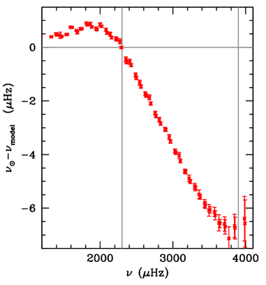
There have been several concerted efforts to improve the near-surface structure of models in order to decrease the surface term. Rosenthal et al. (1995) showed that solar models constructed with non-local mixing length formulation of Gough (1977) as formulated by Balmforth (1992) reduces the surface term with respect to the Sun. Demarque et al. (1997) showed that parametrizing the structure of the super-adiabatic layer in simulations and applying that to solar models improves frequencies. Other efforts include patching the results of realistic convection simulations on stellar models (e.g. Rosenthal et al., 1999; Piau et al., 2014; Jørgensen et al., 2018). Houdek et al. (2017) did a detailed study of the physics ingredients that contribute to the surface term, and they confirmed that there are multiple sources, including effects from convection dynamics; they show that the surface term can indeed be made negligibly small. There work, however, was done with solar envelope models and therefore, do not easily translate to models along an evolutionary sequence. As a step in this direction, (Mosumgaard et al., 2018) have been examining models constructed with near-surface properties obtained by interpolating withing grids of convection simulations. However, these models still show a surface term, probably because Mosumgaard et al. (2018) neglected turbulent pressure. However, it is not enough to include turbulent pressure in the models; Sonoi et al. (2017) showed that to achieve the best results, perturbations to turbulent pressure must be taken into account properly when frequencies of such models are calculated. Thus even as there are ongoing efforts to improve the near-surface properties of stellar models, the vast majority of stellar models used have a substantial surface term that needs to be accounted for properly.

For helioseismic studies, where many hundreds of modes are available, the problem of the surface term is handled by relying on frequency inversions rather than frequency comparisons (see Basu 2016 and references therein). The inversion process explicitly accounts for the surface term (e.g., Dziembowski et al., 1990, 1991; Däppen et al., 1991; Antia & Basu, 1994) and thus does not depend on correcting the frequencies. However, the dearth of asteroseismic data (tens of frequencies rather than hundreds) along with a lack of independent constraints on mass, radius and age, make inversions impractical for most stars. As a result, other strategies are required; these involve either subtracting out the surface term, making it less effective, or using a different observable related to the frequencies.

The most common way of removing the effect of the surface term is to assume that it has a known functional form and subtract it our from the frequency differences between a star and its model. Most early analyses used the surface term correction proposed by Kjeldsen et al. (2008). That form assumes that the frequency difference caused by near-surface effects can be expressed as a power-law in frequency, with the exponent determined from a solar surface term. While this form is easy to use, it depends on the surface term between the Sun and a solar model, and that depends on the physics of the solar model. Additionally, it can be shown (Schmitt & Basu 2015) that this form does not work very well for frequencies far away from $\nu_{\rm max}$, nor does it work too well for models of stars more evolved that the Sun. As a result, it is increasingly common to use the form proposed by Ball & Gizon (2014) based on an idea of Gough (1990). They proposed that the surface term could be fit to the form

$$\delta\nu_{nl}=\nu_{nl}^{\rm obs}-\nu_{nl}^{\rm model}=\frac{1}{I_{nl}}\left[a\left(\frac{\nu_{nl}}{\nu_{\rm ac}}\right)^{-1}+b\left(\frac{\nu}{\nu_{\rm ac}}\right)^{3}\right],$$ (1)

where $\delta\nu_{nl}$ is the difference in frequency for a mode of degree $l$ order $n$ between a star and its model, $\nu_{nl}$ is the frequency and $I_{nl}$ is the inertia of the mode, and $\nu_{\rm ac}$ is the acoustic cut-off frequency. The coefficients $a$ and $b$ can be determined through a generalized linear least-squares fit (see Howe et al., 2017). The biggest advantage of this form is that one does not have to rely on a solar model to fix the parameters. The explicit dependence on mode inertia also implies that no special treatment is needed to to use the correction on non-radial modes. This correction works quite well in general, and we show this in the left column of Fig. 2 where we have corrected the frequencies of the standard solar model shown in Fig. 1; for this purpose we used set of solar frequencies degraded to match what is obtained for other stars with Kepler. Both corrected and uncorrected frequencies are shown for comparison.

Figure 2: Echelle diagram showing solar frequencies (black/gray) as well as the uncorrected (blue) and corrected (red) frequencies of the SSM BS05(OP) of Bahcall et al. (2005) (left), and the best-fit model obtained using the correction in Eq. 1 (right). The solar frequencies used are BiSON data degraded to stellar levels by Lund et al. (2017) and used by Silva Aguirre et al. (2017).

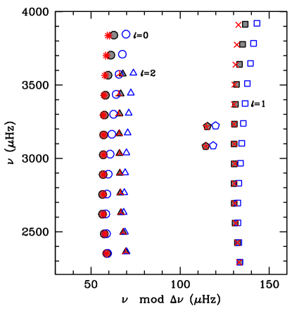
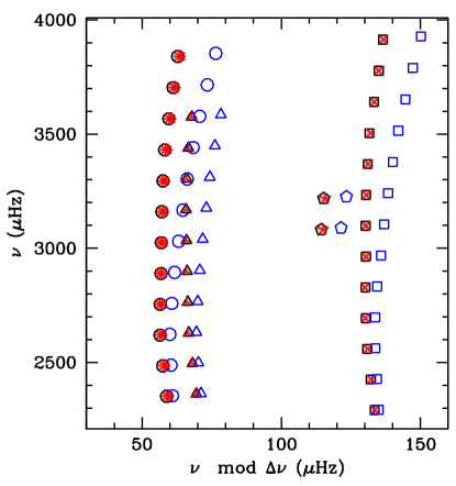
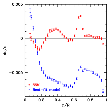
The problem with Eq. 1 is that it can over-correct the frequencies and remove differences that are caused by differences in the structure of deeper layers. We show this in the right column of Fig. 2, where the corrected and uncorrected frequencies of a model with $M/M_{\odot}=1.0142$, $R/R_{\odot}=1.01$, $T_{\rm eff}=5779$ K and and age of 4.87 Gyr are plotted; we refer to this model as the “best-fit”model. The corrected frequencies appear to fit the solar data better than those of the standard solar model, however the internal structure of best-fit model has a much larger mismatch with the Sun than the SSM. This is shown in Fig. 3. Thus clearly, the surface-term correction is giving us misleading results.

Figure 3: The sound-speed difference between the Sun and the SSM BS05(OP) (red) and the best-fit model (blue). The solar results are from Basu et al. (2009). The errors bars show $3\sigma$ uncertainty.

As mentioned earlier, it is not usually possible to invert stellar frequencies to determine the difference in structure between star and its model (see Bellinger et al. 2017 for recent attempts, successes and limitations), and we therefore need other means to judge the mismatch between the internal structures of stars and their models. One such way is to look at specific frequency combinations, usually called separation ratios. The usual ones are

$$r_{01}(n)=\frac{d\nu_{01}(n)}{\nu_{n,1}-\nu_{n-1,1}},\quad\quad r_{10}(n)=\frac{d\nu_{10}(n)}{\nu_{n+1,0}-\nu_{n,0}},$$ (2)

where,

$$d\nu_{01}(n) = \nu_{n,0}-\frac{1}{2}\left(\nu_{n-1,1}+\nu_{n,1}\right),$$

$$d\nu_{10}(n) = \frac{1}{2}\left(\nu_{n,0}+\nu_{n+1,0}\right)-\nu_{n,1},$$ (3)

When plotted against frequency, $d\nu_{01}$ and $d\nu_{10}$ are not usually smooth and thus sometimes higher order differences are used to define the separations (e.g., Roxburgh 2009, Silva Aguirre et al. 2011, Silva Aguirre et al. 2015). Another combination used extensively is

$$r_{02}=\frac{\nu_{n+1,0}-\nu_{n,2}}{\nu_{n,1}-\nu_{n-1,1}}.$$ (4)

The ratio $r_{02}$ is sensitive to the central hydrogen concentration, and hence age, of a star on the main sequence (Christensen-Dalsgaard, 1988).

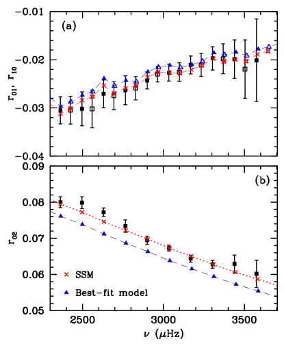
The separation ratios in Eq. 2, and Eq. 4 are quite insensitive to the surface term (see Roxburgh, 2004, 2005; Otí Floranes et al., 2005). In Fig. 4 we compare the frequency ratios of the SSM and best-fit models with those of the Sun, and can be seen clearly, the best-fit model does not really fit the ratios, in particular the mismatch is very large for $r_{02}$; this is of course expected since $r_{02}$ is sensitive to the age of a star, and the best-fit model has the wrong age. Thus had we used the ratios to determine a best-fit model, we would not chosen this one.

Figure 4: The separation ratios $r_{01}$, $r_{10}$ (panel a) and $r_{02}$ (panel b) of the Sun (points with error bars), the SSM (red crosses) and the best-fit model (blue triangles). The ratios for the models have been connected with a line to guide the eye.

The insensitivity of the separation ratios to the surface term have led to the creation of asteroseismic analysis pipeline that depend only on the separation ratios and not the individual frequencies (see e.g., BASTA, Silva Aguirre et al. 2015) though the precision of results obtained with frequency rations appears to be smaller than those obtained with frequencies explicitly corrected for the surface term (see e.g., Silva Aguirre et al., 2017). One complicating factor in using the frequency ratios is error-correlations. Errors for $r_{01}(n)$ and $r_{10}(n)$ are highly correlated, as are errors between neighboring ratios of a given type, e.g., between $r_{01}(n)$ and $r_{01}(n+1)$. Definitions of $r_{01}$ and $r_{10}$ that involve higher order differences are correlated over many more data points. The errors of neighboring $r_{02}$ are also correlated. These correlations follow from the definition of the ratios.

Another quantity that can help in determining whether a model matches a star is the phase factor $\epsilon$ defined as:

$$\nu=\langle\Delta\nu\rangle\left(n+\frac{l}{2}+\epsilon\right),$$ (5)

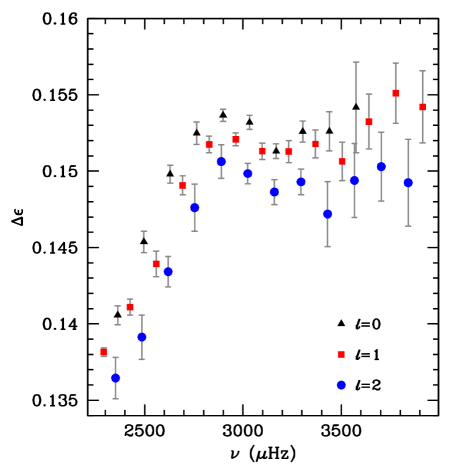
where $\langle\Delta\nu\rangle$ is the average large separation. It can be shown that is the internal structure of a model matches that of a star, the difference in $\epsilon$ between then is independent of degree and is a function of frequency alone (Roxburgh, 2015). Fig. 5 shows the differences in $\epsilon$ between the Sun and the best-fit model; the differences are clearly degree dependent. Roxburgh (2015) demonstrated that $\epsilon$ differences can be used to determine the characteristics of a star.

Figure 5: The difference in $\epsilon$ between Sun and the best-fit model. Note that at any given frequency, the differences are degree dependent.

Thus clearly the surface term correction can end up giving us misleading results about a star. It is worth noting, however, that while the best-fit model differs from the Sun in internal structure, the global parameters of the model are not wildly different. The mass of the best-fit models differs from that of the Sun by only only 1.4%, radius by 1%, the difference in $T_{\rm eff}$ is negligible. The only major difference is in age, but that is only a 6.5% difference, much better than what is obtained by non-asteroseismic studies, even of star clusters. Thus the question is whether this means that despite limitations of the surface term, we can determine robust global properties of stars using their oscillation frequencies. This is the question we try to answer in this paper. The global properties of stars are what is use by the wider astronomy community for their work and hence, it is important to examine the sensitivity of the results to the ubiquitous surface term.

We use all the three techniques — explicit correction of the surface term using Eq. 1, the use of frequency ratios, and the use of $\epsilon$ differences to examine whether the global properties of the stars are indeed determined robustly despite the problem of the surface term. We start with the Sun, and both components of the 16 Cyg system. These are three stars with the most well-determined oscillation frequencies. In order to be sure that the quality of the data of these stars is not misleading us, we analyze three other stars, KIC 6106415 (HD 177153), KIC 6225718 (HD 187637), and KIC 8006161 (HIP 91949).

3 The analysis techniques

We estimate the global properties of the stars we are studying by statistical analyses of a large ensemble of models. We determine the likelihood of each model and the final parameters are the likelihood-weighted average of the underlying properties of the models. What differs in each case what quantity is used to define the likelihood. Since we do not have evidence to the contrary, all inputs are assumed to have a Gaussian distribution of errors that allows us to define a $\chi^{2}$ value for each input.

We start with the method of $\epsilon$ differences. For each model we calculate the difference in $\epsilon$ between the star and the model, with the differences being calculated at the observed frequencies, i.e.,

$$\Delta\epsilon_{nl}=\epsilon^{\rm obs}(\nu^{\rm obs}_{nl})-\epsilon^{\rm model}(\nu^{\rm obs}_{nl}),$$ (6)

where, $\epsilon^{\rm model}(\nu^{\rm obs}_{nl})$ is $\epsilon$ for the model at degree $l$ interpolated to the observed frequency $\nu^{\rm obs}_{nl}$ of the same degree $l$. To determine whether or not the $\epsilon$ differences are a function of frequency alone, we define an arbitrary function of frequency ${\mathcal{F}}=\sum_{i}^{M}a_{i}\phi(\nu)_{i}$, where $\phi(\nu)$ are basis functions in frequency. We then minimize

$$\chi^{2}(\epsilon)=\frac{1}{N-M}\sum_{nl}\left(\frac{\Delta\epsilon_{nl}-{\mathcal{F}}(\nu^{\rm obs}_{nl})}{S^{\rm obs}_{nl}}\right),$$ (7)

where $N$ is the total number of models, $M$ the number of basis function (chosen to be fewer than the number of radial modes as per the suggestion of Roxburgh 2015), and $S^{\rm obs}_{nl}=\sigma^{\rm obs}_{nl}/\Delta\nu^{\rm obs}$, with $\sigma^{\rm obs}_{nl}$ being the uncertainty on $\nu^{\rm obs}_{nl}$. We use B-spline basis functions. A small value of $\chi^{2}(\epsilon)$ indicates that the $\epsilon$ differences are a function of frequency alone. We then define the likelihood of any given model as

$${\mathcal{L}}(\epsilon)=A\exp\left(-\frac{\chi^{2}(\epsilon)}{2}\right),$$ (8)

$A$ being a normalization factor such that $\sum{\mathcal{L}}(\epsilon)=1$ with the sum taken over all models.

Next, we consider frequency ratios. To avoid large error-correlations we only use ratios $r_{01}$ and $r_{02}$ as define in Eqs. 2 and 4. We do not use $r_{10}$, and we neglect the error correlations between $r_{01}$ and $r_{02}$. We then define the likelihood for $r_{01}$ as

$$\chi^{2}(r_{01})=({\mkern 1.5mu\overline{\mkern-1.5mur_{01}\mkern-1.5mu}\mkern 1.5mu}^{({\rm obs})}-{\mkern 1.5mu\overline{\mkern-1.5mur_{01}\mkern-1.5mu}\mkern 1.5mu}^{({\rm model})})^{T}{\mathbf{C}}^{-1}({\mkern 1.5mu\overline{\mkern-1.5mur_{01}\mkern-1.5mu}\mkern 1.5mu}^{({\rm obs})}-{\mkern 1.5mu\overline{\mkern-1.5mur_{01}\mkern-1.5mu}\mkern 1.5mu}^{({\rm model})}),$$ (9)

where ${\mkern 1.5mu\overline{\mkern-1.5mur_{01}\mkern-1.5mu}\mkern 1.5mu}({\rm obs})$ is the vector defining the observe $r_{01}$, ${\mkern 1.5mu\overline{\mkern-1.5mur_{01}\mkern-1.5mu}\mkern 1.5mu}({\rm model})$ is the vector defining the $r_{01}$ for the model at the observed frequency, and ${\mathbf{C}}$ is the error-covariance matrix. Thus ${\mathcal{L}}(r_{01})=B\exp(-\chi^{2}(r_{01})/2)$. We define ${\mathcal{L}}(r_{02})$ in an analogous manner, and thus for the two ratios taken together

$${\mathcal{L}}({\rm rat})={\mathcal{L}}(r_{01}){\mathcal{L}}(r_{02}).$$ (10)

The third way of analyzing the models was to use surface-term corrected frequencies of the models. We define $\nu^{\rm corr}_{nl}=\nu_{nl}^{\rm model}-S$, where $S$ is defined by the right-hand side of Eq. 1. We can then define

$$\chi^{2}(\nu)=\frac{1}{N-2}\sum_{nl}\frac{(\nu_{nl}^{\rm obs}-\nu_{nl}^{\rm corr})^{2}}{\sigma^{\rm obs}_{nl}},$$ (11)

and consequently

$${\mathcal{L}}(\nu)=C\exp\left(-\frac{\chi^{2}(\nu)}{2}\right),$$ (12)

$C$ being the normalization constant.

The surface term is expected to be smaller at low frequencies and larger at high frequencies, however, for models that do not fit the data very well, the frequency differences can show the opposite behavior. We weigh against such models by defining a weight ${\mathcal{W}}({\rm low})$ where

$${\mathcal{W}}_{\rm low}=\exp\left(-\frac{\chi^{2}_{\rm low}}{2}\right),$$ (13)

where $\chi^{2}_{\rm low}$ is the $\chi^{2}$ for the (uncorrected) frequency differences between the two lowest frequency radial modes.

It is usual to consider the observed $T_{\rm eff}$ and metallicity in the analyses, and we have analyzed the models with and without constraints on $T_{\rm eff}$ and metallicity. The likelihood for $T_{\rm eff}$ is defined as

$${\mathcal{L}}(T)=D\exp(-\chi^{2}(T)/2),$$ (14)

with

$$\chi^{2}(T)=\frac{(T^{\rm obs}_{\rm eff}-T^{\rm model}_{\rm eff})^{2}}{\sigma^{2}_{T}},$$ (15)

where $\sigma_{T}$ is the uncertainty on the effective temperature, we consider two cases, $\sigma_{T}=100$K and $\sigma_{\rm T}=50$. We similarly define a likelihood ${\mathcal{L}}({\mathrm{[Fe/H]}})$ and again we consider two different uncertainties, $\sigma_{\mathrm{[Fe/H]}}=0.1$ dex and $\sigma_{\mathrm{[Fe/H]}}=0.05$ dex.

For some cases we also apply a weight for age. The equations of stellar structure and evolution do not know anything about the age of the universe, and thus in principle, a model could gave an age greater than that of the universe. While a model older than the age of the universe is unphysical, uncertainties in mass, metallicity and effective temperature could easily result in such a model. Instead of removing all models above an age of 13.8 Gyr (which would result in a sharp cut-off in the probability density function of age) we use a weight for age $\tau$ defined as

$${\mathcal{W}}_{\rm age}=\begin{cases}1,&\hbox{if}\;\;\tau<=13.8\;\hbox{Gyr}\\ \exp\left[-\frac{(13.8-\tau)^{2}}{2\sigma^{2}_{\tau}}\right]&\hbox{otherwise},\\ \end{cases}$$ (16)

$\tau$ is in units of Gigayears, and $\sigma_{\tau}$ is chosen to be 0.1 Gyr.

In Table 1 we list all the different parameter combinations that we have used to determine the global properties of the stars under question. Method 1 simply means that we calculate the likelihood of a model only with $\epsilon$, i.e., we only calculate ${\mathcal{L}}({\rm total})={\mathcal{L}}(\epsilon)$, in Method 2, it is calculated as ${\mathcal{L}}({\rm total})={\mathcal{W}}_{\rm age}{\mathcal{L}}(\epsilon)$, in Method 3 corresponds to ${\mathcal{L}}({\rm total})={\mathcal{L}}(\epsilon){\mathcal{L}}(T){\mathcal{L}}(\hbox{[Fe/H]})$, etc.

Table 1: The different combinations of observables used in the analysis

Method No.	Observables used	Notes
11	$\epsilon$
12	$\epsilon$	additional weights for age using ${\mathcal{W}}_{\rm age}$
13	$\epsilon$, $T_{\rm eff}$, $\mathrm{[Fe/H]}$	using $\sigma_{T}=100$K and $\sigma_{\mathrm{[Fe/H]}}=0.1$ dex
14	$\epsilon$, $T_{\rm eff}$, $\mathrm{[Fe/H]}$	using $\sigma_{T}=75$K and $\sigma_{\mathrm{[Fe/H]}}=0.05$ dex
15	$\epsilon$, $T_{\rm eff}$, $\mathrm{[Fe/H]}$	as in Method 4, but weighted for age using ${\mathcal{W}}_{\rm age}$
16	$r_{01},\;r_{02}$
17	$r_{01},\;r_{02}$	additional weights for age using ${\mathcal{W}}_{\rm age}$
18	$r_{01},\;r_{02}$, $T_{\rm eff}$, $\mathrm{[Fe/H]}$	using $\sigma_{T}=100$K and $\sigma_{\mathrm{[Fe/H]}}=0.1$ dex
19	$r_{01},\;r_{02}$, $T_{\rm eff}$, $\mathrm{[Fe/H]}$	using $\sigma_{T}=75$K and $\sigma_{\mathrm{[Fe/H]}}=0.05$ dex
10	$r_{01},\;r_{02}$, $T_{\rm eff}$, $\mathrm{[Fe/H]}$	as in Method 9, but weighted for age using ${\mathcal{W}}_{\rm age}$
11	$\nu$
12	$\nu$	additional weights for age using ${\mathcal{W}}_{\rm age}$
13	$\nu$, $T_{\rm eff}$, $\mathrm{[Fe/H]}$	using $\sigma_{T}=100$K and $\sigma_{\mathrm{[Fe/H]}}=0.1$ dex
14	$\nu$, $T_{\rm eff}$, $\mathrm{[Fe/H]}$	using $\sigma_{T}=75$K and $\sigma_{\mathrm{[Fe/H]}}=0.05$ dex
15	$\nu$, $T_{\rm eff}$, $\mathrm{[Fe/H]}$	as in Method 14, but weighted for age using ${\mathcal{W}}_{\rm age}$
16	$\nu$, $T_{\rm eff}$, $\mathrm{[Fe/H]}$	as in Method 15, but with additional weight ${\mathcal{W}}_{\rm low}$

4 The data

Table 2: Average seismic parameters and surface properties

Star	$\Delta\nu$	$\nu_{\rm max}$	$T_{\rm eff}$	$\mathrm{[Fe/H]}$
	($\mu$ Hz)	($\mu$ Hz)	(K)
Sun	$134.91\pm 0.02$	$3073\pm 13$	$5772\pm 10$	$0.0\pm 0.0$
16 Cyg A	$103.28\pm 0.02$	$2188\pm 5$	$5825\pm 50$	$0.01\pm 0.03$
16 Cyg B	$116.93\pm 0.02$	$2561\pm 5$	$5750\pm 50$	$0.05\pm 0.02$
KIC 6106415	$104.07\pm 0.03$	$2249\pm 5$	$6037\pm 77$	$-0.04\pm 0.1$
KIC 6225718	$105.07\pm 0.02$	$2364\pm 5$	$6313\pm 77$	$-0.07\pm 0.1$
KIC 8006161	$149.43\pm 0.02$	$3575\pm 11$	$5488\pm 77$	$0.34\pm 0.1$

We analyze six stars in this paper. The first three, the Sun, 16 Cyg A and 16 Cyg B not only have precise data on frequencies, they also have precise data on their effective temperatures and metallicities. For the Sun, we use the degraded solar frequencies used by Silva Aguirre et al. (2017) as obtained by Lund et al. (2017). For each star, we use frequencies, large separations and $\nu_{\rm max}$ values from Lund et al. (2017), although for $\Delta\nu$ and $\nu_{\rm max}$, we assume that the uncertainty is the larger of the two limits provided. We analyze three others stars: KIC 6106415 (HD 177153), KIC 6225718 (HD 187637), and KIC 8006161 (HIP 91949). The frequencies of these stars are not as precise as those of the others, and the $T_{\rm eff}$ and $\mathrm{[Fe/H]}$ values are not known as precisely as those of the other stars either. The results for these stars allow us to judge the dependence of our results on the quality of the data. For the Sun, we assume the $T_{\rm eff}$ value of Mamajek et al. (2015). For the components of the 16 Cyg system we use $T_{\rm eff}$ and $\mathrm{[Fe/H]}$ from Ramírez et al. (2009), KIC 6106415, KIC 6225718 and KIC 8006161 we use $\mathrm{[Fe/H]}$ from Buchhave & Latham (2015) and temperatures derived by Buchhave & Latham as listed in Mathur et al. (2017). Table 2 lists the average seismic properties, $T_{\rm eff}$ and $\mathrm{[Fe/H]}$ of the stars being studied.

5 Construction of stellar models

We constructed a large number of models for each star with YREC, the Yale stellar evolution code (Demarque et al., 2008). The models were constructed with the OPAL equation of state (Rogers & Nayfonov, 2002). OPAL opacities (Iglesias & Rogers, 1996) supplemented with low-temperature opacities from Ferguson et al. (2005) were used. We used the NACRE reaction rates from Angulo et al. (1999) except for the ${}^{14}N(p,\gamma)^{15}O$ reaction, where we used the rates of Marta et al. (2008). We included diffusion and settling of heavy elements using the coefficients of Thoul et al. (1994). To avoid the problem of heavy-elements draining out of the outer convection zones of hot stars in an unphysical manner, we artificially reduced the diffusion coefficients as a function of total mass as:

$$C_{\rm diff}=\begin{cases}1,&\hbox{if}\;\;M<=1.25\\ \exp\left[-\frac{(M-1.25)^{2}}{2(0.085)^{2}}\right]&\hbox{otherwise},\\ \end{cases}$$ (17)

where $M$ is the mass of the model in units of M_⊙, and $C_{\rm diff}$ a multiplicative factor for the Thoul et al. (1994) diffusion coefficients.

Table 3: Range of $T_{\rm eff}$ and initial $\mathrm{[Fe/H]}$ of models

Star	$T_{\rm eff}$	$\mathrm{[Fe/H]}$
	(K)
Sun	5550–5950	$-0.33$–$0.47$
16 Cyg A	5640–6040	$-0.20$–$0.60$
16 Cyg B	5610–6010	$-0.25$–$0.55$
KIC 6106415	5730–6345	$-0.30$–$0.40$
KIC 6225718	6005–6620	$-0.10$–$0.70$
KIC 8006161	5180–5800	$\phantom{-}0.10$–$0.80$

We start the modelling process with the observed $\Delta\nu$, $\nu_{\rm max}$, $T_{\rm eff}$, and $\mathrm{[Fe/H]}$ of each star, along with their uncertainties. Using these we created many realizations of the four quantities. For $\Delta\nu$, and $\nu_{\rm max}$, we assumed that the realizations have a Gaussian distribution with a $\sigma$ of four times the uncertainty in each quantity. We assumed flat distributions for $T_{\rm eff}$and $\mathrm{[Fe/H]}$. Since the observed $\mathrm{[Fe/H]}$ is the present day metallicity, we assumed that the initial metallicity was about 0.1 dex higher than the present one for the purpose of constructing models. The spread in current $T_{\rm eff}$ and initial $\mathrm{[Fe/H]}$ for models of each star are listed in Table 3. For the initial helium abundance $Y_{0}$ we assumed a flat distribution between $0.24$ and $0.34$. The initial $\mathrm{[Fe/H]}$ was converted to initial hydrogen abundance $X_{0}$ and heavy-element abundance $Z_{0}$ using the initial $Y_{0}$ assuming the Grevesse & Sauval (1998) solar metallicity scale, i.e., $\hbox{[Fe/H]}=0\equiv Z/X=0.023$.

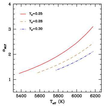
For any given realization, we have a set of parameters ($\Delta\nu$, $\nu_{\rm max}$, $T_{\rm eff}$, $X_{0}$, $Z_{0}$, $Y_{0}$). For each set, $\Delta\nu$ and $\nu_{\rm max}$ were converted to mass $M$ and radius $R$ using the asteroseismic scaling relations corrected as per the prescription of Guggenberger et al. (2016). This gave us sets of ($M$, $R$, $T_{\rm eff}$, $X_{0}$, $Z_{0}$), where $M$, $X_{0}$, $Z_{0}$ are inputs to the models and we want a model of radius $R$ at the specified $T_{\rm eff}$ to be the output. This is done by using YREC in an iterative manner where we iterate over $\alpha_{\rm MLT}$, the mixing length parameter, until we obtain a models that has the required radius at the specified $T_{\rm eff}$. The condition on the observed present-day metallicity is applied post facto when we use Methods 3–5, 8–10, and 13-16 to analyze the ensemble of models; it is ignored otherwise. In Fig. 6 we show an example of how $\alpha_{\rm MLT}$ has to change with $T_{\rm eff}$ in order for a 1M_⊙ model to have a radius of 1R_⊙ at that value of $T_{\rm eff}$.

Figure 6: The mixing-length parameters $\alpha_{\rm MLT}$ required for a 1M_⊙, $\mathrm{[Fe/H]}$=0 model to have a radius of 1R_⊙ at different values of $T_{\rm eff}$. We show the case for three different values of $Y_{0}$. Unlike rest of the models used in this work, models in this figure were constructed without diffusion and settling of heavy elements to ensure that the models have the exact value of the current surface metallicity.

The frequencies of each model were calculated using the code of Antia & Basu (1994) and were then used to calculate $\epsilon$, and frequency ratios $r_{01}$ and $r_{02}$. For models of any given star, we only used those modes that have been observed. The frequency difference of each model with respect to the observed frequencies were fitted to the Ball & Gizon form (Eq. 1) to determine the surface-term corrected frequencies. The ensemble of models of each star were then analyzed using different measures as listed in Table 1.

6 Results

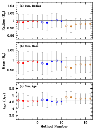
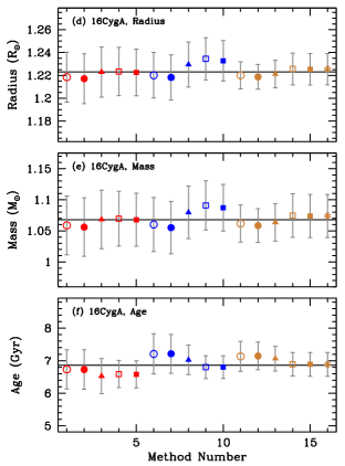
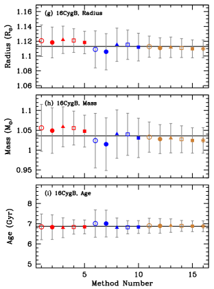
The mass, radius and age of the Sun, and the two components of the 16 Cyg system as derived using the sixteen different combinations are shown in Fig. 7. It is very clear from the figure that central value of the estimates (i.e., the likelihood weighted means) are very similar in each case. The uncertainty on the results on the other hand, are somewhat different. The methods that explicitly use the surface-term corrected frequencies appear to have the lowest uncertainties, however, at least for the Sun where we have independent measures of mass and radius, the surface-term corrected frequencies give the largest systematic errors. But in all cases, the results are well within 1$\sigma$ of the actual value. Unlike radius and mass, age uncertainties are lowered considerably when $T_{\rm eff}$ and $\mathrm{[Fe/H]}$ are considered explicitly — not surprising since the age of a model at a given mass and radius depends critically on its temperature and metallicity. It should be noted that all results presented here are consistent with those of Silva Aguirre et al. (2017).

Figure 7: Estimates of mass, radius and age of the Sun, 16 Cyg A and 16 Cyg B obtained using goodness-of-fit measures to different observables as listed in Table 1. The numbers on the abscissa refer to the method number in the table. Red, blue and orange points denote the fact that the seismic variable used is $\epsilon$, frequency ratios and surface-term corrected frequencies respectively. The horizontal lines for the solar case are the known solar values. For the other cases we plot the mean of the results obtained. The vertical extent of the panels shows a fixed fraction of the values — $\pm 5$% for radius, $\pm 10$% for mass, and $\pm 30$% for age — to give an indication of the precision of the estimates.

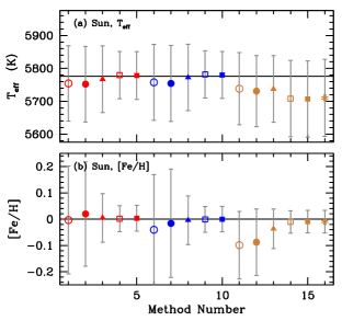
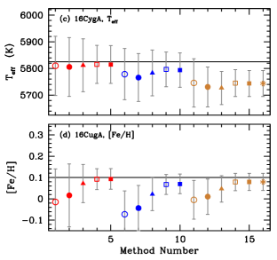
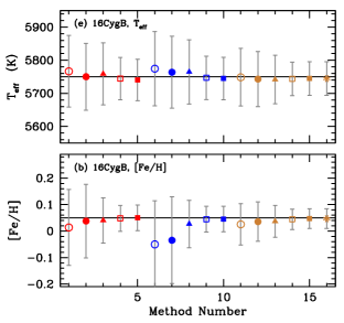
Asteroseismic analyses use $T_{\rm eff}$ and $\mathrm{[Fe/H]}$ to complement the data set, however, we attempted to examine how well we could estimate the temperature and metallicity of stars from seismic data alone. The results for the Sun and the 16 Cyg system are shown in Fig. 8. We find that temperature can be localized to better than $\pm 100$K when no constraint is applied, when we do apply a temperature constraint, we find that we recover temperature to about $\pm 70$K regardless of whether we assumed a Gaussian spread of 100 K or 75 K. We should note however, that although we assumed a flat prior in temperature, the models were restricted to a finite (400 K) range in temperature, and that could have an effect on the final spread of the results. Metallicity results are worse; unless we apply a constraint, we can recover $\mathrm{[Fe/H]}$ to only between 0.1 and 0.2 dex. We get more precise results when the explicit surface-term corrections are used, but judging by the solar case, that can result in larger systematic errors.

Figure 8: $T_{\rm eff}$ and $\mathrm{[Fe/H]}$ for the Sun, 16 Cyg A and 16 Cyg B. In the panels that show results for the Sun, the horizontal line marks the known solar value; in the other panels the line is simply an arithmetic average of all the results shown in the panel.

Figure 9: The initial helium abundance and the current convection-zone helium abundance of the Sun. The solid horizontal line in each panel marks the helioseismically determine value of that quantity — $Y_{0}$ from Serenelli & Basu (2010) and $Y_{\rm CZ}$ from Basu (1998). Dotted lines show 1$\sigma$ uncertainties of the helioseismic estimates.

Figure 10: The initial helium and heavy-element abundance of 16 Cyg A (large red points) and 16 Cyg B (small blue points).

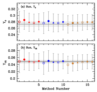
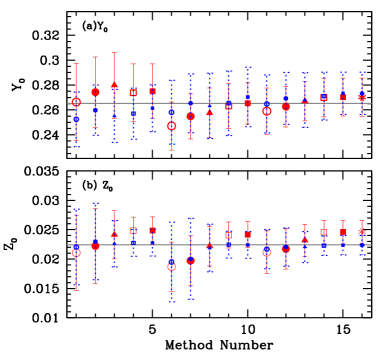
For the Sun, we find that no matter which method we use, we can reproduce the helioseismically determined initial helium abundance of the Sun (Serenelli & Basu, 2010) as well the current convection-zone helium abundance for the Sun (see Basu, 1998). These are shown in Fig. 9. The precision for $Y_{0}$ is however, a factor of five worse than that obtained from the detailed helioseismic study. The uncertainty in $Y_{\rm CZ}$ is a factor of ten worse. However, the difference between $Y_{0}$ and $Y_{\rm CZ}$ does give a good estimate of the amount of helium that has settled out of the convection zone. The analysis of the two components of the 16 Cyg system shows that estimates of $Y_{0}$ and $Z_{0}$ are the same for both components of the system (Fig. 10) even though we did not take into account the fact that the two stars should have the same initial composition.

Figure 11: Mass, radius and age estimates for KIC 6106415, KIC 6225718 and KIC 8006161. The colors are the same as in Fig. 7 The horizontal line in each panel is the average of all the values in that panel.

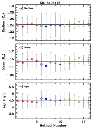
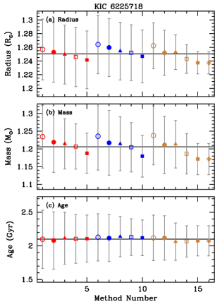
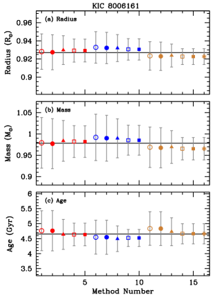
The Sun and the two stellar components of the 16 Cyg system have the most precisely determined frequencies, and this leads to the question of what happens if the frequency-set is not as extensive, or if the errors on the modes larger. To answer this we analyzed the data of the other three stars and the results are shown in Fig. 11. As as be seen, the results obtained for a given star with using the different asteroseismic parameters are consistent with each other, and all results agree well within 1$\sigma$ of each other. The worse precision of the frequency-sets of these stars caused the worse precision of the results for these stars; the best precision is obtained when the frequencies are explicitly corrected for the surface term, but as before there there could be a larger systematic error in this case, which we have no means of evaluating independently.

Figure 12: The initial helium abundance $Y_{0}$ and initial heavy-element abundance $Z_{0}$ of KIC 6106415, KIC 6225718 and KIC 8006161. The colors are the same as in Fig. 7 The horizontal line in each panel is the average of all the values in the panel.

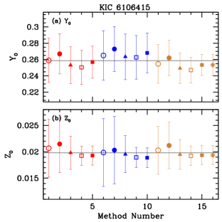
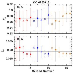
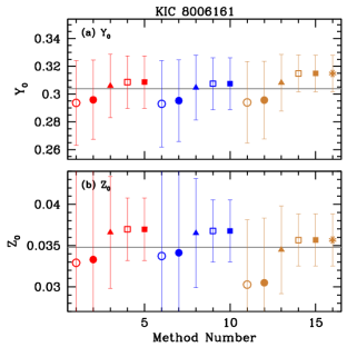
Estimates of $Y_{0}$ and $Z_{0}$ for KIC 6106415, KIC 6225718 and KIC 8006161 are different though. The spread in values is much larger (see Fig. 12), particularly for KIC 6225718 and KIC 8006161, the two stars with comparatively larger frequency uncertainties. However, the results are still the same within 1$\sigma$, except that $\sigma$ is large. For these stars, meaningful results for $Z_{0}$ are obtained only for cases where $T_{\rm eff}$ and surface metallicity are explicitly taken into account in the analysis.

Table 4: Spread in results (in percent) caused by different ways of handling the surface term. The Method numbers are the same as those in Table 4

Methods	% Spread in stellar-parameter estimates
compared	Mass	Radius	Age	$Y_{0}$	$Z_{0}$
1, 16, 11	1.1	0.45	2.7	2.6	6.1
2, 17, 12	1.1	0.45	2.8	2.5	6.3
3, 18, 13	1.0	0.40	2.9	2.9	2.9
4, 19, 14	1.2	0.46	1.9	2.5	1.4
5, 10, 15	1.1	0.42	1.9	2.3	1.3

The spread in the global parameters obtained using the different ways of accounting for the surface term is listed in Table 4. The different rows correspond to analyses when different non-seismic constraints were used. The first row, for example, looks at the spread in results when no non-seismic constraint was used. As can be seen, the change in radius is typically less than 0.5% and the change in mass is about 1%. These numbers are smaller than the typical uncertainties in mass and radius caused by uncertainties in asteroseismic and spectroscopic data (see e.g., Metcalfe et al., 2014; Silva Aguirre et al., 2015, 2017) The effect on ages is larger and depends on whether or not $T_{\rm eff}$ and $\mathrm{[Fe/H]}$ have been use, and the effect is at the 2-3% level, much smaller than the usual uncertainties in age. The effect on $Y_{0}$ is very similar to that on age. As far as $Z_{0}$ is concerned, the effect of the surface term appears to be tied to whether or not $\mathrm{[Fe/H]}$ is used as a constraint, and the spread can be as high as 6% when $\mathrm{[Fe/H]}$ is not used to constrain the results. We should emphasize that the seeming insensitivity of the results to the way the surface term is accounted for does not mean that we have the option to ignore it altogether. When a sufficient number of modes is available (as is the case of the six stars that have been showcased in this investigation) the $\chi^{2}$ for the best fit to the frequencies without a surface term correction is very large. This occurs because models that give a good fit to the low-frequency modes, do not fit the high frequency modes, and vice versa. Models that give better fits to the low-frequency have properties that are closer to that of the star than models that fit the high frequency end. This is a result of the fact that the change in frequency due to the surface term increases with mode frequency. The more problematic case is when modes are available only over a small frequency range (2–3 $\Delta\nu$) around $\nu_{\rm max}$, in that case one can get a good fit in terms of $\chi^{2}$, but the chances of fitting a model with wrong parameters is high. Thus without a proper accounting of the surface term, the results obtained will not be reliable.

In this work we have not tested the effect of systematic errors in $T_{\rm eff}$ and $\mathrm{[Fe/H]}$. However, a simple analyses of the solar case shows that in the event that the systematic error in temperature is of the order of uncertainties in temperature, the effect on mass is no more than 1%, and the effect on radius is much lower. The effect in age however, can be larger, of the order of a few per cent. The effect of metallicity errors is slightly larger. These effects are being examined in detail in a separate investigation (Bellinger et al. in preparation).

7 Discussion and Conclusions

We have demonstrated that how the surface term in asteroseismic data is accounted for does not affect estimates of the mass, radius or age of a star. No matter how the surface term is dealt with, whether by bypassing the term issue completely by using $\epsilon$, minimizing its contribution using ratios, or explicitly removing it using a model for the surface term, we get very consistent results for the most important global properties of the stars. The spread in mass because of the different ways of constraining the surface term is only about 1%, the spread is radius is less than 0.5%, while the spread in age, when $T_{\rm eff}$ and $\mathrm{[Fe/H]}$ is used is about 2%. All these are lower than the typical uncertainties in this quantities caused by data errors. Meaningful estimates of initial helium and metallicity require a knowledge of the effective temperature and current metallicity of the stars; once the spectroscopic data are taken into account, the results are robust with small enough uncertainties to make the results meaningful.

We used all available radial, dipole and quadrupole modes for the stars studied in this paper. We did not use octopole modes even when available since they can observed in very few stars from photometric data. The robustness of the results to surface term corrections hold as long as we have enough modes of each degree to determine if $\epsilon$ has a degree-dependence, which means that we need modes of at least two different degrees, or that we have enough modes to calculate a sufficient number of frequency ratios $r_{01}$ and $r_{02}$. Mode sets with as few as four to five orders per degree give good results. The range of frequencies covered by the available modes available does not matter for the $\epsilon$-matching or the ratios method, however, it is important when the surface term is calculated explicitly. The Ball & Gizon (2014) formulation and the Kjeldsen et al. (2008) formulation can only be fitted over a limited frequency range. The very low frequency range where surface term corrections are small ($\lesssim 2000\;\mu$Hz for the solar case, see Fig. 1), or at high frequencies where the surface term turns over ($\gtrsim 4000\;\mu$Hz for the solar case), are fitted badly by these forms. For these regions other forms of the surface term need to be used. One can, for instance, explicitly use the scaled solar surface term as was done by the “ASFIT” and “YMCM” analyses described in Appendix A of Silva Aguirre et al. (2015). However, with photometry measurements, the likelihood of obtaining frequencies so low that the functional forms do not apply is small since the signal from granulation masks the modes, and high-frequency modes usually have large enough uncertainties that they do not play much of a role in determining stellar properties.

All six stars in our sample are main sequence stars. A valid question to ask is what happens to more evolved stars, particularly to subgiants. We do not expect the results to be significantly different from what we have found for the main sequence stars. The p-mode frequencies of subgiants are affected by the surface term the same way as the p modes of main sequence stars. Given that the radius and mass of stars can be estimated precisely with only average asteroseismic parameters $\Delta\nu$ and $\nu_{\rm max}$(see e.g. Gai et al., 2011), the pure p modes of subgiants stars are enough to determine radius and mass precisely, and thus these quantities will should only be affected to the same extent as those for main sequence stars. Age is a somewhat different issue. If we look for age precision at the same level as those for main sequence stars, then the results of this work should apply even for evolved stars. However, much more precise ages can be obtained for subgiants if mixed-mode frequencies are used (Metcalfe et al., 2010; Deheuvels & Michel, 2011). The frequency of mixed modes is a very sensitive function of age, and thus the broad-brush statistical technique is not the best if we are to determine the age of a subgiant to the precision that is possible. To get the better results, we need to start with the best-fit stellar parameters that fit the p-modes and search around that. Since mixed modes have high inertia, and thus less affected by surface effects, we expect the final result to be insensitive to how the surface term in p modes was removed. However, on the red giant branch where all dipole modes are mixed modes, the usual surface term corrections may not apply at all (Ball et al., 2018) and the situation will be very different, unless we confine ourselves to only using the radial and quadrupole modes. The expected results for subgiants and red giants need to be tested properly with real data.

It should be noted that our results pertain to the effects of the surface term alone, the model dependence of the different estimates is beyond the scope of this paper. In particular, one needs to keep in mind that age estimates of stars are always model dependent.

References

- Angulo et al. (1999) Angulo, C., Arnould, M., Rayet, M., et al. 1999, Nuclear Physics A, 656, 3
- Antia & Basu (1994) Antia, H. M., & Basu, S. 1994, A&AS, 107, 421
- Arnett et al. (2010) Arnett, D., Meakin, C., & Young, P. A. 2010, Astrophys. J., 710, 1619
- Bahcall et al. (2005) Bahcall, J. N., Serenelli, A. M., & Basu, S. 2005, ApJ, 621, L85
- Ball & Gizon (2014) Ball, W. H., & Gizon, L. 2014, A&A, 568, A123
- Ball et al. (2018) Ball, W. H., Themeßl, N., & Hekker, S. 2018, MNRAS, 478, 4697
- Balmforth (1992) Balmforth, N. J. 1992, MNRAS, 255, 639
- Basu (1998) Basu, S. 1998, MNRAS, 298, 719
- Basu (2016) —. 2016, Living Reviews in Solar Physics, 13, 2
- Basu & Chaplin (2017) Basu, S., & Chaplin, W. J. 2017, Asteroseismic Data Analysis: Foundations and Techniques, Princeton Series in Modern Observational Astronomy Series (Princeton University Press)
- Basu et al. (2009) Basu, S., Chaplin, W. J., Elsworth, Y., New, R., & Serenelli, A. M. 2009, ApJ, 699, 1403
- Basu et al. (1996) Basu, S., Christensen-Dalsgaard, J., Perez Hernandez, F., & Thompson, M. J. 1996, MNRAS, 280, 651
- Bellinger et al. (2017) Bellinger, E. P., Basu, S., Hekker, S., & Ball, W. H. 2017, ApJ, 851, 80
- Böhm-Vitense (1958) Böhm-Vitense, E. 1958, Z. Astrophys., 46, 108
- Brown (1984) Brown, T. M. 1984, Science, 226, 687
- Buchhave & Latham (2015) Buchhave, L. A., & Latham, D. W. 2015, ApJ, 808, 187
- Canuto & Mazzitelli (1991) Canuto, V. M., & Mazzitelli, I. 1991, Astrophys. J., 370, 295
- Chaplin et al. (2007) Chaplin, W. J., Serenelli, A. M., Basu, S., et al. 2007, ApJ, 670, 872
- Chaplin et al. (2014) Chaplin, W. J., Basu, S., Huber, D., et al. 2014, ApJS, 210, 1
- Christensen-Dalsgaard (1988) Christensen-Dalsgaard, J. 1988, in IAU Symposium, Vol. 123, Advances in Helio- and Asteroseismology, ed. J. Christensen-Dalsgaard & S. Frandsen, 295
- Christensen-Dalsgaard et al. (1988) Christensen-Dalsgaard, J., Dappen, W., & Lebreton, Y. 1988, Nature, 336, 634
- Däppen et al. (1991) Däppen, W., Gough, D. O., Kosovichev, A. G., & Thompson, M. J. 1991, in Lecture Notes in Physics, Berlin Springer Verlag, Vol. 388, Challenges to Theories of the Structure of Moderate-Mass Stars, ed. D. Gough & J. Toomre, 111
- Deheuvels & Michel (2011) Deheuvels, S., & Michel, E. 2011, A&A, 535, A91
- Demarque et al. (1997) Demarque, P., Guenther, D. B., & Kim, Y.-C. 1997, ApJ, 474, 790
- Demarque et al. (2008) Demarque, P., Guenther, D. B., Li, L. H., Mazumdar, A., & Straka, C. W. 2008, Ap&SS, 316, 31
- Dziembowski et al. (1991) Dziembowski, W. A., Pamiatnykh, A. A., & Sienkiewicz, R. . 1991, MNRAS, 249, 602
- Dziembowski et al. (1990) Dziembowski, W. A., Pamyatnykh, A. A., & Sienkiewicz, R. 1990, MNRAS, 244, 542
- Ferguson et al. (2005) Ferguson, J. W., Alexander, D. R., Allard, F., et al. 2005, ApJ, 623, 585
- Gai et al. (2011) Gai, N., Basu, S., Chaplin, W. J., & Elsworth, Y. 2011, ApJ, 730, 63
- Gough (1977) Gough, D. O. 1977, ApJ, 214, 196
- Gough (1990) Gough, D. O. 1990, in Lecture Notes in Physics, Berlin Springer Verlag, Vol. 367, Progress of Seismology of the Sun and Stars, ed. Y. Osaki & H. Shibahashi, 283
- Grevesse & Sauval (1998) Grevesse, N., & Sauval, A. J. 1998, Space Sci. Rev., 85, 161
- Guggenberger et al. (2016) Guggenberger, E., Hekker, S., Basu, S., & Bellinger, E. 2016, MNRAS, 460, 4277
- Houdek et al. (2017) Houdek, G., Trampedach, R., Aarslev, M. J., & Christensen-Dalsgaard, J. 2017, MNRAS, 464, L124
- Howe et al. (2017) Howe, R., Basu, S., Davies, G. R., et al. 2017, MNRAS, 464, 4777
- Iglesias & Rogers (1996) Iglesias, C. A., & Rogers, F. J. 1996, ApJ, 464, 943
- Jørgensen et al. (2018) Jørgensen, A. C. S., Mosumgaard, J. R., Weiss, A., Silva Aguirre, V., & Christensen-Dalsgaard, J. 2018, MNRAS, 481, L35
- Kjeldsen et al. (2008) Kjeldsen, H., Bedding, T. R., & Christensen-Dalsgaard, J. 2008, ApJ, 683, L175
- Lebreton et al. (2014) Lebreton, Y., Goupil, M. J., & Montalbán, J. 2014, in EAS Publications Series, Vol. 65, EAS Publications Series, 99–176
- Lund et al. (2017) Lund, M. N., Silva Aguirre, V., Davies, G. R., et al. 2017, ApJ, 835, 172
- Mamajek et al. (2015) Mamajek, E. E., Prsa, A., Torres, G., et al. 2015
- Marta et al. (2008) Marta, M., Formicola, A., Gyürky, G., et al. 2008, Phys. Rev. C, 78, 022802
- Mathur et al. (2012) Mathur, S., Metcalfe, T. S., Woitaszek, M., et al. 2012, ApJ, 749, 152
- Mathur et al. (2017) Mathur, S., Huber, D., Batalha, N. M., et al. 2017, ApJS, 229, 30
- Metcalfe et al. (2010) Metcalfe, T. S., Monteiro, M. J. P. F. G., Thompson, M. J., et al. 2010, ApJ, 723, 1583
- Metcalfe et al. (2014) Metcalfe, T. S., Creevey, O. L., Doğan, G., et al. 2014, ApJS, 214, 27
- Mosumgaard et al. (2018) Mosumgaard, J. R., Ball, W. H., Silva Aguirre, V., Weiss, A., & Christensen-Dalsgaard, J. 2018, MNRAS, 478, 5650
- Nordlund & Stein (1997) Nordlund, A., & Stein, R. 1997, in Astrophysics and Space Science Library, Vol. 225, SCORe’96 : Solar Convection and Oscillations and their Relationship, ed. F. P. Pijpers, J. Christensen-Dalsgaard, & C. S. Rosenthal, 79–103
- Otí Floranes et al. (2005) Otí Floranes, H., Christensen-Dalsgaard, J., & Thompson, M. J. 2005, MNRAS, 356, 671
- Piau et al. (2014) Piau, L., Collet, R., Stein, R. F., et al. 2014, MNRAS, 437, 164
- Pinsonneault et al. (2014) Pinsonneault, M. H., Elsworth, Y., Epstein, C., et al. 2014, ApJS, 215, 19
- Pinsonneault et al. (2018) Pinsonneault, M. H., Elsworth, Y. P., Tayar, J., et al. 2018
- Ramírez et al. (2009) Ramírez, I., Meléndez, J., & Asplund, M. 2009, A&A, 508, L17
- Rogers & Nayfonov (2002) Rogers, F. J., & Nayfonov, A. 2002, ApJ, 576, 1064
- Rosenthal et al. (1995) Rosenthal, C. S., Christensen-Dalsgaard, J., Houdek, G., et al. 1995, in ESA Special Publication, Vol. 376, Helioseismology, 459–464
- Rosenthal et al. (1999) Rosenthal, C. S., Christensen-Dalsgaard, J., Nordlund, Å., Stein, R. F., & Trampedach, R. 1999, A&A, 351, 689
- Roxburgh (2004) Roxburgh, I. W. 2004, in ESA Special Publication, Vol. 538, Stellar Structure and Habitable Planet Finding, ed. F. Favata, S. Aigrain, & A. Wilson, 23–36
- Roxburgh (2005) Roxburgh, I. W. 2005, A&A, 434, 665
- Roxburgh (2009) —. 2009, A&A, 493, 185
- Roxburgh (2015) —. 2015, A&A, 574, A45
- Schmitt & Basu (2015) Schmitt, J. R., & Basu, S. 2015, ApJ, 808, 123
- Serenelli et al. (2017) Serenelli, A., Johnson, J., Huber, D., et al. 2017, ApJS, 233, 23
- Serenelli & Basu (2010) Serenelli, A. M., & Basu, S. 2010, ApJ, 719, 865
- Silva Aguirre et al. (2011) Silva Aguirre, V., Ballot, J., Serenelli, A. M., & Weiss, A. 2011, A&A, 529, A63
- Silva Aguirre et al. (2015) Silva Aguirre, V., Davies, G. R., Basu, S., et al. 2015, MNRAS, 452, 2127
- Silva Aguirre et al. (2017) Silva Aguirre, V., Lund, M. N., Antia, H. M., et al. 2017, ApJ, 835, 173
- Sonoi et al. (2017) Sonoi, T., Belkacem, K., Dupret, M.-A., et al. 2017, A&A, 600, A31
- Stein & Nordlund (1998) Stein, R. F., & Nordlund, Å. 1998, ApJ, 499, 914
- Tanner et al. (2013) Tanner, J. D., Basu, S., & Demarque, P. 2013, ApJ, 767, 78
- Thoul et al. (1994) Thoul, A. A., Bahcall, J. N., & Loeb, A. 1994, ApJ, 421, 828
- Townsend et al. (2018) Townsend, R. H. D., Goldstein, J., & Zweibel, E. G. 2018, MNRAS, 475, 879