Axion global fits with Peccei-Quinn symmetry breaking before inflation using GAMBIT

Abstract

We present global fits of cosmologically stable axion-like particle and QCD axion models in the mass range 0.1 neV to 10 eV. We focus on the case where the Peccei-Quinn symmetry is broken before the end of inflation, such that the initial value of the axion field can be considered to be homogeneous throughout the visible Universe. We include detailed likelihood functions from light-shining-through-wall experiments, haloscopes, helioscopes, the axion relic density, horizontal branch stars, supernova 1987A, white dwarf cooling, and gamma-ray observations. We carry out both frequentist and Bayesian analyses, with and without the inclusion of white dwarf cooling. We explore the degree of fine-tuning present in different models and identify parameter regions where it is possible for QCD axion models to account for both the dark matter in the Universe and the cooling hints, comparing them to specific DFSZ- and KSVZ-type models. We find the most credible parameter regions, allowing us to set (prior-dependent) upper and lower bounds on the axion mass. Our analysis also suggests that QCD axions in this scenario most probably make up a non-negligible but sub-dominant component of the dark matter in the Universe.

1 Introduction

QCD axions 1977_pq_axion1 ; 1977_pq_axion2 ; 1978_weinberg_axion ; 1978_wilczek_axion and axion-like particles (ALPs) are perhaps among the most intriguing classes of hypothetical particles. They have been extensively studied in the literature and experiments are expected to probe the relevant parameter space for many axion models in the near future (see Ref. 1801.08127 for an up-to-date review on axion searches). Because QCD axions can behave as cold dark matter (DM) Preskill:1982cy ; Abbott:1982af ; Dine:1982ah ; 1986_turner_axiondensity , the particularly interesting regions of the parameter space are where they contribute significantly to the DM density of the Universe. If so, they would solve at least two outstanding problems in physics at the same time (the other being the Strong CP problem 1977_pq_axion1 ; 1977_pq_axion2 ).

There are now many complementary searches for axions underway, and many new search strategies have emerged in recent years (see Ref. 1801.08127 ). Axions could also explain some apparent anomalies in the cooling of white dwarf stars Isern:1992gia ; 1205.6180 ; 1211.3389 ; 1512.08108 ; 1605.06458 ; 1605.07668 ; 1708.02111 , or the transparency of the Universe to gamma rays 0707.4312 ; 0712.2825 ; 1001.0972 ; 1106.1132 ; 1201.4711 ; 1302.1208 . It is therefore crucial to combine all available results in order to extract the maximum information from the data. In doing so, we can learn more about the parameter space of different models, help guide the planning of future searches towards the most promising search areas and – if axions do indeed exist – find them in the correlated signals of several experiments and determine their properties.

Some of these goals can be satisfactorily achieved by over-plotting exclusion limits from several experiments. However, such simple exclusion plots generally have some shortcomings. They make assumptions about the relative importance of interactions with other matter, and about important inputs such as solar physics, the local density of DM and theoretical uncertainties. Incompatibilities between the assumptions can undermine the validity of a simple combination. They also do not allow for a quantitative model comparison between different theories that include axions.

A solution is to perform a consistent global statistical analysis of all available constraints, accounting for the leading theoretical and experimental uncertainties. Implementing such an analysis requires careful design, along with compromises relating to the availability of data and the total computational runtime required. An example of such a computational framework for BSM physics is GAMBIT gambit . Full details of GAMBIT’s features can be found in the relevant publications gambit ; ColliderBit ; DarkBit ; FlavBit ; SDPBit ; ScannerBit and physics analyses MSSM ; SSDM ; CMSSM ; SSDM2 ; HiggsPortal ; EWMSSM . The most relevant features for this work are GAMBIT’s modularity, and the options that it offers for carrying out both Bayesian and frequentist analyses. GAMBIT’s structure allows easy integration of new components such as models, theory calculations, likelihoods and sampling algorithms. GAMBIT contains a variety of advanced samplers for both Bayesian and frequentist analyses, which are particularly useful for including nuisance parameters and assessing fine-tuning.

In the following section, we review some aspects of axion physics, including specific issues that should be accounted for in global fits. In Sec. 3, we turn to axion models, their corresponding effective field theories and the family tree of axion models available in GAMBIT. Sec. 4 describes our observables and likelihood functions, including their implementation, incorporated experimental data, potential caveats and restrictions. Results and discussion of the first global scans of axion models can be found in Sec. 5, and Sec. 6 summarises our results.

The axion routines developed for this paper are available in the DarkBit DarkBit module of GAMBIT 1.3.1, available at https://gambit.hepforge.org under the 3-clause BSD license. Likelihood and posterior samples from this study can be downloaded from Zenodo Zenodo_axions .

2 Axion physics

Here we present a brief overview of axion physics, highlighting caveats of our current implementation and pointing out opportunities for future extensions. More details can be found in the literature 1987_kim_lightpseudoscalars ; Kuster:2008zz ; 1201.5902 ; 1301.1123 ; 1510.07633 ; 1801.08127 .

2.1 The QCD axion

The Peccei-Quinn (PQ) mechanism 1977_pq_axion1 ; 1977_pq_axion2 is a proposed solution to the Strong CP problem that gives rise to a pseudo-scalar particle: the QCD axion 1978_weinberg_axion ; 1978_wilczek_axion . The QCD axion is an excellent DM candidate Preskill:1982cy ; Abbott:1982af ; Dine:1982ah ; 1986_turner_axiondensity , as it can account for the entire cosmological abundance of DM via the vacuum misalignment or realignment mechanism (Sec. 2.3.1). The original QCD axion model also inspired further archetypical models, such as the KSVZ 1979_kim_ksvz ; 1980_shifman_ksvz and DFSZ 1980_zhitnitsky_dfsz ; 1981_dine_dfsz axion models, which we will introduce in Secs 3.2.1 and 3.2.2.

The symmetries of the Standard Model (SM) Lagrangian permit a term of the form

$$\pazocal{L}_{\text{QCD}}\supset-\frac{\alpha_{\text{S}}}{8\pi}\theta_{\text{QCD}}G_{\mu\nu}^{a}\widetilde{G}^{\mu\nu,a}\,,$$ (1)

where $G_{\mu\nu}^{a}$ is the gluon field strength, $a$ is the $SU(3)$ gauge index and $\alpha_{\text{S}}$ is the strong coupling constant. The angle $\theta_{\text{QCD}}\in[-\pi,\pi]$ is an unknown parameter and $\widetilde{G}^{\mu\nu,a}=\epsilon^{\mu\nu\kappa\lambda}G_{\kappa\lambda}^{a}/2$. A contribution is also generated by chiral transformations due to the chiral anomaly, which replaces $\theta_{\text{QCD}}$ by an effective angle,

$$\theta_{\text{eff}}\equiv\theta_{\text{QCD}}-\arg\left[\det(Y_{d}Y_{u})\right]\,,$$ (2)

where $Y_{d}$ and $Y_{u}$ are the down- and up-type Yukawa matrices, respectively (Book_2014_Schwartz, , Sec. 29.5). The $G\widetilde{G}$-term is anti-symmetric under the discrete parity ($P$) and charge-parity ($CP$) transformations. Due to the presence of this term, one would naïvely expect the strong interaction to show some $CP$-violating effects – especially because weak interactions are known to violate $P$ maximally and $CP$ mildly. There is no $CP$-violation if and only if $\theta_{\text{eff}}$ vanishes (modulo the periodicity).

Experiments trying to measure the CP-violating electric dipole moment of the neutron (nEDM) can place limits on the value of $\theta_{\text{eff}}$. Within 40–50% uncertainty, the dipole moment induced by the $G\widetilde{G}$-term is given by 1979_crewther ; 1980_crewther ; hep-ph/9904483

$$|d_{n}|\approx\left($2.4\text{\times}{10}^{-16}\text{\,}\mathrm{\text{ $e$ }}\text{\,}\mathrm{cm}$\right)\left|\theta_{\text{eff}}\right|\,.$$ (3)

The current limit on the nEDM is $|d_{n}|<$3.6\text{\times}{10}^{-26}\text{\,}\mathrm{\text{ $e$ }}\text{\,}\mathrm{cm}$$ at 95% confidence level 1509.04411 , resulting in $|\theta_{\text{eff}}|\mathrel{\hbox to0.0pt{\lower 4.0pt\hbox{$\sim$}\hss}\raise 1.0pt\hbox{$<$}}${10}^{-10}$$.

This observation poses a fine-tuning issue in the SM, commonly referred to as the Strong CP problem. The mechanism suggested by Peccei and Quinn 1977_pq_axion1 ; 1977_pq_axion2 solves this problem by introducing a new global, axial $U(1)$ symmetry. This so-called PQ symmetry is spontaneously broken by the vacuum expectation value $v$ of a complex scalar field. The resulting Nabu-Goldstone boson is the QCD axion, a pseudo-scalar field denoted by $a(x)$. It adds another contribution to $\theta_{\text{eff}}$ of the form $Na(x)/v$, where the non-zero integer $N$ is the colour anomaly of the PQ symmetry. The associated shift symmetry can then be used to cancel the $\theta_{\text{eff}}$ term by driving $\theta_{\text{eff}}+Na(x)/v$ to zero. In fact, it can be shown by the Vafa-Witten theorem 1984_vafa_vafawitten1 ; 1984_vafa_vafawitten2 that the axion dynamically and asymptotically relaxes $\theta_{\text{eff}}$ to the $CP$-conserving minimum. The Strong CP problem is therefore effectively solved by promoting $\theta_{\text{eff}}$ to a dynamical degree of freedom.

The continuous shift symmetry of the PQ $U(1)$ phase forbids any mass terms for the axion at the Lagrangian level. In the presence of an $a\,G\widetilde{G}$ term in the Lagrangian, however, this symmetry is broken after the QCD phase transition due to topologically non-trivial fluctuations of the gluon fields, leaving only a discrete shift symmetry of size $2\pi Nv$.

The resulting effective potential can be written as

$$V(a)=f_{a}^{2}\,m_{a}^{2}\,\left[1-\cos(a/f_{a})\right]\,,$$ (4)

where $m_{a}$ is the temperature-dependent axion mass and $f_{a}\equiv v/N$. The axion is therefore practically massless until the time of the QCD phase transition, where it picks up a small mass that can be calculated using the chiral Lagrangian formalism.

The zero-temperature mass of the QCD axion was initially calculated by relating $v$ to the scale of weak interactions 1978_weinberg_axion . However, this model was ruled out and the parameter space for $f_{a}$ was opened up in order to make the axion “invisible” – in the sense that it evaded experimental constraints at the time. Neglecting suppressed quark mass ratios, the QCD axion mass at zero temperature is given by 1978_weinberg_axion

$$m_{a,0}\simeq\frac{\sqrt{z_{d}}}{1+z_{d}}\,\frac{f_{\pi^{0}}}{f_{a}}\,m_{\pi^{0}}\,,$$ (5)

where $z_{d}=m_{u}/m_{d}$ is the up- and down-quark mass ratio, and $f_{\pi^{0}}$ and $m_{\pi^{0}}$ are the decay constant and mass of the pion respectively. Using next-to-leading order chiral perturbation theory, a recent study found the QCD axion mass at zero temperature to be 1511.02867

$$m_{a,0}=$5.70(7)\text{\,}\mathrm{\SIUnitSymbolMicro eV}$\left(\frac{${10}^{12}\text{\,}\mathrm{GeV}$}{f_{a}}\right)\,.$$ (6)

At temperatures exceeding the QCD scale, the axion becomes increasingly light as the shift symmetry is restored. Numerical estimates of the temperature dependence can be obtained directly from recent lattice QCD simulations 1606.03145 ; 1606.07494 . These results are well-approximated at higher temperatures by a power law $m_{a}(T)\propto T^{-\beta/2}$ for some $\beta>0$, and by a constant axion mass below some transition temperature $T_{\chi}$. This also agrees with the behaviour predicted from the finite-temperature dilute instanton gas approximation 1980_Pisarski .

As we solve all relevant equations numerically in this paper, it would be straightforward to include the full lattice QCD results and calculate the axion mass at every given temperature. However, including the statistical uncertainties is most easily achieved by having a parametrised form of the temperature dependence of the QCD axion mass. This is commonly done by introducing two parameters, $\beta$ and $T_{\chi}$, which we fit to lattice QCD results. More details about the implementation can be found in Sec. 3.2.

2.2 Axion-like particles

Apart from the original QCD axion, pseudo-Nambu-Goldstone bosons with fundamental shift symmetries appear in many other contexts. These are usually referred to as ALPs (axion-like particles), and are appealing for theorists and model builders because of the shift symmetry, and the ability of their field values to undergo relaxation via the realignment mechanism in the same manner as axions. They do not necessarily solve the Strong CP problem. However, under the right circumstances, they can be cold DM candidates, or play an important role in solving other physics puzzles. ALPs typically arise from the breaking of a $U(1)$ symmetry at some scale $f_{a}$ and generate a mass from explicit breaking of the residual symmetry at scale $\Lambda$. As a result, they can be fairly light, with masses of the order $m_{a}\sim\Lambda^{2}\left/f_{a}\right.$, and have suppressed couplings to the SM. Due to the lack of a direct relation between the two scales involved ($f_{a}$ and $m_{a}$), they occupy a larger parameter space than QCD axions. More details on the theory and phenomenology of these particles can be found in the literature 1987_kim_lightpseudoscalars ; 1002.0329 ; 1801.08127 .

2.3 Axion creation mechanisms

QCD axions (with roughly $\mathrm{\SIUnitSymbolMicro eV}$ to $\mathrm{meV}$ masses) and many ALP models are expected to be lighter than other hypothetical particles, such as WIMPs, which typically have $\mathrm{GeV}$ to $\mathrm{TeV}$-scale masses 1003.0904 . For thermal DM, this would be problematic, as DM would not be sufficiently cold today to reproduce the observed large-scale structure of the Universe. However, although a small population of axions is produced thermally, the relic abundance is typically dominated by non-thermal mechanisms, namely the realignment mechanism and topological defects. In this work, we focus on the realignment mechanism, which allows axions to be both ultra-cold and very light at the same time.

2.3.1 Realignment mechanism

The equation of motion for a homogeneous QCD axion or ALP field $\theta(t)=a(t)/f_{a}$ with potential $V(\theta)$ in a Friedmann-Robertson-Walker-Lemaître universe reads (weinberg_cosmology, , app. B.12)

$$\ddot{\theta}+3H(t)\dot{\theta}+\frac{1}{f_{a}^{2}}\frac{\delta V(\theta)}{\delta\theta}=0\,,$$ (7)

where $H\equiv\dot{a}/a$ is the Hubble parameter. For the canonical axion potential,

$$V(\theta)=f_{a}^{2}m_{a}^{2}\left[1-\cos(\theta)\right],$$ (8)

the equation of motion becomes

$$\ddot{\theta}+3H(t)\,\dot{\theta}+m_{a}^{2}(t)\,\sin(\theta)=0\,.$$ (9)

The general form of this equation does not possess analytic solutions. In the early Universe $m_{a}\ll H$ and the system is an overdamped oscillator. We can integrate the differential equation with boundary conditions $\theta(t_{\text{i}})=\theta_{\text{i}}$ and $\dot{\theta}(t_{\text{i}})=0$, where the value $\theta_{\text{i}}$ of the axion field is called the initial misalignment angle.

At later times, around the time when $m_{a}\sim H$, the system becomes critically damped and the field starts to oscillate. In the regime of $m_{a}\gg H$, the axion field oscillations are adiabatic while their amplitude continuously decreases due to Hubble damping. In other words, at some time $t_{\star}$, the axion field evolution is guaranteed to eventually enter an epoch where $\left|\theta(t)\right|\ll 1$ for all $t>t_{\star}$. In this harmonic limit, (9) is a damped harmonic oscillator, and the field evolution is very well described by the WKB approximation 1201.5902

$$\theta(t)\propto\left[m_{a}(t)\;a^{3}(t)\right]^{-\frac{1}{2}}\cos\left(\int^{t}_{t_{\star}}\!m_{a}(\tau)\,\mathrm{d}\tau+\delta_{\star}\right),$$ (10)

where we can match the solution at time $t_{\star}$ with the phase $\delta_{\star}$. This limiting form of the axion scalar field oscillations can be used to demonstrate that they behave like cold DM at sufficiently late times by averaging (10) over an oscillation period to find the effective behaviour of the energy density, $\varepsilon$, such that 1201.5902

$$\langle\varepsilon\rangle\propto m_{a}\;a^{-3}\,.$$ (11)

Once the mass becomes constant, this is the scaling behaviour of cold matter. We can rephrase this statement for non-relativistic axions to see that the (averaged) comoving axion number density is conserved:

$$n^{\text{com}}_{a}\equiv\frac{\rho a^{3}}{m_{a}}\simeq\frac{\varepsilon a^{3}}{m_{a}}\,.$$ (12)

In fact, there is an adiabatic invariant in the harmonic limit of $\sin(\theta)\simeq\theta$, which has been studied in the literature for QCD axions and ALPs Abbott:1982af ; 1986_turner_axiondensity ; Frieman:1991qv . However, if the initial misalignment angle $\theta_{\text{i}}\sim\pazocal{O}(1)$, then the adiabatic invariant is not sufficient to describe the system, and anharmonic effects arising from the full potential must be taken into account. These have been estimated and calculated by several authors 1986_turner_axiondensity ; Lyth:1991ub ; astro-ph/9405028 ; 0806.0497 ; 0910.1066 .

The energy density in axions today can hence be parametrised by an overall transfer function $F$, with the properties that $F$ is bounded from below, and becomes constant in the harmonic limit $|\theta_{\text{i}}|\ll 1$ 1986_turner_axiondensity ; astro-ph/9405028 ; 0806.0497 . This allows us to conveniently write the axion energy density in the Universe today as

$$\rho_{a}=F\left(|\theta_{\text{i}}|\,;\,\beta,\,T_{\chi},\,m_{a,0}\right)\,\theta_{\text{i}}^{2}\,,$$ (13)

where we explicitly denote the dependence of the transfer function $F$ on the values of the axion parameters. For a given set of these parameters, the transfer function – and hence the axion relic density – could be determined once and used in subsequent calculations. For sampling over the parameter space, it is necessary to repeat this process for each set of parameters (or to tabulate the results on a sufficiently dense grid ahead of the scan).

We have thus far only considered the homogeneous field equation (9). It is not obvious that this is sufficient for determining the energy density in axions today. Let us consider the two possible scenarios in a cosmology with inflation: either PQ symmetry breaks after inflation, or it breaks before inflation ends.

In the first case, the Universe consists of a large number of causally disconnected “bubbles” where the initial misalignment angles take random values from a uniform distribution on the interval $-\pi$ to $\pi$ 1986_turner_axiondensity . As a consequence, the initial misalignment angle $\theta_{\text{i}}$ effectively becomes a function of space. Nonetheless, the resulting overall energy density in axions is fixed, because it can be calculated as the average over all the misalignment angles in all the patches. As $\theta_{\text{i}}$ is constant within the patches, we may use (13) to calculate the result:

$$\rho_{a}^{\text{post-inf}}=\frac{1}{2\pi}\,\int_{-\pi}^{\pi}\!F\left(|\theta_{\text{i}}|\right)\theta_{\text{i}}^{2}\,\mathrm{d}\theta_{\text{i}}=\frac{1}{\pi}\,\int_{0}^{\pi}\!F\left(|\theta_{\text{i}}|\right)\theta_{\text{i}}^{2}\,\mathrm{d}\theta_{\text{i}}\,.$$ (14)

In the second case, where the PQ symmetry breaks before the end of inflation, one causally connected patch gets blown up to at least the size of the observable Universe. The axion field is therefore homogeneous, with a random initial value in the interval $(-\pi,\pi]$. The stochastic nature of the initial misalignment angle gives rise to a physically motivated prior probability for $\theta_{\text{i}}$ in a Bayesian analysis, which will be discussed in Sec. 5.

A major issue with this scenario is perturbations from inflation, which will affect the initial misalignment angle by some amount that depends on the energy scale of inflation (see e.g. Lyth:1991ub, ). It has been argued that this scenario is therefore finely-tuned to a degree that can be considered “worse” than the Strong CP problem itself 0911.0418 ; 0911.0421 . Since the necessary additional implementation of inflationary models is beyond the scope of this work, we neglect the issue of field fluctuations during inflation.

2.3.2 Topological defects

Because axions arise from the breaking of a $U(1)$ symmetry, topological defects known as cosmic strings and domain walls can appear Kibble:1976sj ; book_kolbturner . Decay of these defects to axions will increase the axion DM density. They have been studied extensively in the literature, but the relative importance of their contribution is still not firmly established Davis:1985pt ; Davis:1986xc ; Harari:1987ht ; Hagmann:1990mj ; astro-ph/9311017 ; astro-ph/9403018 ; hep-ph/9807428 ; hep-ph/9811311 ; hep-ph/0012361 ; 1202.5851 ; 1012.4558 ; 1012.5502 ; 1412.0789 ; 1509.00026 ; 1707.05566 ; 1708.07521 ; 1806.04677 .

Some authors have parametrised the topological defect contribution as $\Omega_{a}=\Omega_{a}^{\mathrm{realign}}(1+\alpha)$, where $\Omega_{a}^{\mathrm{realign}}$ is the contribution from realignment. Including $\alpha$ as a nuisance parameter in our work would remove much of the predictability of the model, and would assume similar scaling of the energy density contributions. As we consider PQ symmetry to break before inflation, we assume that contributions from topological defects are diluted away during inflation astro-ph/0610440 .

2.3.3 Thermal creation

Axions are also thermally produced in the early Universe 1987_Turner ; book_kolbturner . The resulting abundance is however rather dependent on the additional new field content associated with the axion.

For the QCD axion, the Boltzmann equations for the least model-dependent processes give useful estimates. The contributions of low-temperature processes such as $\pi+\pi\rightleftharpoons\pi+a$ have been computed 1987_Turner ; book_kolbturner ; hep-ph/9306216 ; hep-ph/0504059 , including all combinations of pionic states $\pi$. Thermal axion production during reheating has also been studied hep-ph/0203221 ; 1008.4528 ; 1310.6982 . As hadronisation would not yet have taken place by the time of reheating, these calculations consider processes like axion-gluon interactions, i.e. $g+g\rightleftharpoons g+a$. Recent calculations also considered model-dependent processes with quarks $q$, i.e. $q+\bar{q}\rightleftharpoons g+a$ and $q+g\rightleftharpoons q+a$, which can be dominant in the early Universe 1801.06090 .

A significant abundance of thermal axions modifies the effective number of relativistic species, which can be used to set limits on the axion mass hep-ph/0312154 ; 0705.2695 ; 0706.4198 ; 0803.1585 ; 1004.0695 ; 1307.0615 ; 1403.4852 ; 1503.00911 ; 1507.08665 . Generally speaking, thermally-produced QCD axions with a mass of more than $\pazocal{O}($\mathrm{eV}$)$ are hot DM with a relic abundance comparable to that of neutrinos and photons. Those axion models are therefore excluded, as they would exceed the observational bounds on the fraction of DM that can be hot (e.g. book_kolbturner, ; astro-ph/0610440, ; 1510.07633, ). However, such bounds have some dependence on the choice of cosmological datasets 1503.00911 , and the limits can be relaxed if the Universe had a non-standard thermal history 0711.1352 .

3 Axion models and theoretical uncertainties

Let us now discuss the various axion models that we consider in this work with a focus on the interactions between axions and other particles. We already saw that axions acquire a mass, so that they interact gravitationally. QCD axions also interact via the strong interaction. For generic ALPs, however, it is not clear a priori what the PQ charges of SM particles are, nor whether the axion interacts with a given particle at tree level or only at higher order in perturbation theory.

In order to study axion phenomenology and to identify useful observables, axions have been studied in an effective field theory (EFT) framework Kaplan:1985dv ; 1985_srednicki_axioneft ; 1986_georgi_axioneft , which can be adjusted to a given energy scale and scenario. One can then apply exclusion limits on the effective interactions to specific axion models that establish a relation between the effective couplings and the fundamental axion parameters; examples of such models include the so-called KSVZ model 1979_kim_ksvz ; 1980_shifman_ksvz and the DFSZ model 1980_zhitnitsky_dfsz ; 1981_dine_dfsz .

One important consequence of the fundamental shift symmetry is that axions can only directly interact with matter via derivative couplings. Below the electroweak scale, the effective Lagrangian for axion-SM interactions is

$$\pazocal{L}_{a}=-\sum_{f}\frac{g_{aff}}{2m_{f}}\,\bar{f}\,\gamma^{\mu}\gamma_{5}f\,\partial_{\mu}a-\frac{g_{a\gamma\gamma}}{4}\;aF_{\mu\nu}\widetilde{F}^{\mu\nu}-\frac{\alpha_{\text{S}}}{8\pi}\;\frac{a}{f_{a}}G_{\mu\nu}^{b}\widetilde{G}^{\mu\nu,\,b}\,,$$ (15)

where $a$ is the axion field, $\widetilde{F}$ and $\widetilde{G}$ are the duals of electromagnetic and strong field strengths and $g_{aff}$ and $g_{a\gamma\gamma}$ are effective coupling constants of mass dimension $-1$. In principle, $f$ runs over all SM fermions with mass $m_{f}$, but the couplings most relevant for axion searches are those to electrons and nucleons, the latter arising from matching the EFT to chiral perturbation theory 1986_georgi_axioneft . Also note that the Lagrangian (15) is flavour-diagonal, which is not necessarily the case in all models. While we do not consider the possibility of flavour non-diagonal interactions in this paper, the resulting models can be phenomenologically interesting, rather predictive, and within reach of existing and future experimental searches (e.g. 10.1103/PhysRevLett.49.1549, ; 1612.05492, ; 1612.08040, ).

Figure 1: Family tree of axion models in GAMBIT. The numbers in brackets refer to the number of model parameters; $(n+m)$ indicates $n$ (largely unconstrained) fundamental parameters of the model and $m$ (typically well-constrained) nuisance parameters.

We now turn to the specific axion models implemented in GAMBIT (see Fig. 1). We describe these models in the following subsections, while we leave the discussion of the parameter ranges and prior distributions for Sec. 5. Note that the models presented here are only a subset of the many general and more specific ALP models studied in the literature; detailed overviews can be found in review articles 1510.07633 ; 1801.08127 .

Models in GAMBIT are defined as collections of named parameters. All relevant observables for a model must be computable from these parameters. Models can have relationships to other models, allowing parameter combinations in one model to be translated to equivalent combinations in another model or to an alternative parameterisation of the same model. This is achieved by adding new “children” to the family tree of a more general model and defining a translation between the two models. This translation may, e.g., fix the values of some of the “parent” parameters or compute them as functions of (possibly new) parameters in the child model. This ensures flexibility in the choice of the independent model parameters to work with in any given theory calculation, allowing the most convenient definitions to always be used for any calculation. More details on the general implementation of models in GAMBIT can be found in Ref. gambit .

3.1 General ALP model

We define a new family of GAMBIT models for axions and ALPs. On top of the family tree is the GeneralALP model, with seven parameters. This model describes an effective Lagrangian that is a subset of (15),

$$\pazocal{L}_{a}^{\mathrm{int}}=-\frac{g_{a\gamma\gamma}}{4}aF_{\mu\nu}\widetilde{F}^{\mu\nu}-\frac{g_{aee}}{2m_{e}}\bar{e}\gamma^{\mu}\gamma_{5}e\partial_{\mu}a\,.$$ (16)

In this study we do not include couplings of axions to nucleons. However, future versions of GAMBIT may include additional interactions such as these, subject to the availability of interesting observables and constraints.

We employ the rescaled field value $\theta=a/f_{a}$, assume the canonical cosine potential (8) for all types of axions, and take

$$m_{a}(T)=m_{a,0}\begin{cases}\hfil 1\hfil&\mathrm{if\;}T\leq T_{\chi}\\ \left(\frac{T_{\chi}}{T}\right)^{\beta/2}&\mathrm{otherwise}\end{cases}\,.$$ (17)

A summary of all the model parameters can be found in Table 1.

Table 1: Parameters for the family of axion models. For dimensionful quantities, we also give the units with which they are defined within GAMBIT. The first section refers to parameters that are part of the GeneralALP model. The second section lists the parameters used in child models of the GeneralALP.

Parameter	Description	Comment
$g_{a\gamma\gamma}$	Effective axion-photon coupling	Units of ${\mathrm{GeV}}^{-1}$
$g_{aee}$	Effective axion-electron coupling
$f_{a}$	Axion decay constant	Units of $\mathrm{GeV}$
$m_{a,0}$	Axion zero-temperature mass	Units of $\mathrm{eV}$
$T_{\chi}$	Transition temperature in the broken power law for $m_{a}$	Units of $\mathrm{MeV}$
$\beta$	Exponent of the broken power law for $m_{a}$	$\beta>0$
$\theta_{\text{i}}$	Initial misalignment angle	$-\pi<\theta_{\text{i}}\leq\pi$
$\Lambda$	Breaking scale of the residual symmetry	Units of $\mathrm{MeV}$
$C_{aee}$	Axion-electron coupling
$\Lambda_{\chi}$	Zero-temperature topological susceptibility, $\Lambda_{\chi}^{4}\equiv\chi(T=0)$	Units of $\mathrm{MeV}$
$E/N$	Anomaly ratio in QCD axion models
$\widetilde{C}_{a\gamma\gamma}$	Axion-photon coupling contribution from axion-meson mixing
$\tan(\beta^{\prime})$	Ratio of the two Higgs vacuum expectation values

3.2 QCD axion models

Table 2: Nuisance parameters for the QCD axion model. We only quote best-fit estimates of $\beta$ and $T_{\chi}$, as the likelihood includes correlations between them (cf. Sec. 3.2).

Parameter	Value	Comment
$\Lambda_{\chi}$	$75.5(5)\text{\,}\mathrm{MeV}$	Ref. 1511.02867
$\widetilde{C}_{a\gamma\gamma}$	$1.92(4)$	Ref. 1511.02867
$\beta$	$\hat{\beta}\approx 7.94$	$\left\{\begin{tabular}[]{l}\text{Via lattice QCD nuisance}\\ \text{likelihood based on Ref.\leavevmode\nobreak\ \cite[cite]{\@@bibref{Authors Phrase1YearPhrase2}{1606.07494}{\@@citephrase{(}}{\@@citephrase{)}}}}\end{tabular}\leavevmode\nobreak\ \right.$
$T_{\chi}$	$\hat{T}_{\chi}\approx$147.0\text{\,}\mathrm{MeV}$$

The QCDAxion model is a child of the GeneralALP model. It is inspired by the original QCD axion models, which solve the Strong CP problem. The scale of the explicit breaking of the shift symmetry by instanton-like effects is therefore linked to the QCD scale. This connection can be exploited to uniquely determine the parameters $m_{a,0}$, $\beta$ and $T_{\chi}$. However, there are uncertainties from theory, experiment and lattice QCD simulations that should be taken into account. We treat these as nuisance parameters; Table 2 provides an overview.

Figure 2: Nuisance likelihoods for the scale $\Lambda_{\chi}$ (left, from direct theory calculations 1511.02867 ) and $\beta$ and $T_{\chi}$ (right, from lattice QCD 1606.07494 ). Note that $\beta$ is correlated with $T_{\chi}$ when the full lattice QCD results are taken into account.

Exploiting the connection to QCD, we can replace the parameter $m_{a,0}$ of the GeneralALP model with the energy scale $\Lambda_{\chi}$, defined via the topological susceptibility at zero temperature, $\Lambda_{\chi}^{4}\equiv\chi(T=0)$, such that

$$m_{a,0}\equiv\frac{\Lambda_{\chi}^{2}}{f_{a}}\,.$$ (18)

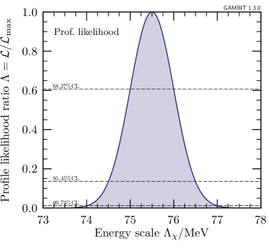
To determine $\Lambda_{\chi}$, we use first principle calculations of the zero-temperature axion mass 1511.02867 . We include these results via a Gaussian likelihood

$$\ln\left(\mathcal{L}\right)=-\frac{1}{2}\frac{(\Lambda_{\chi}-\hat{\Lambda}_{\chi})^{2}}{\sigma_{\Lambda_{\chi}}^{2}}\,,$$ (19)

where $\hat{\Lambda}_{\chi}=$75.5\text{\,}\mathrm{MeV}$$ and $\sigma_{\Lambda_{\chi}}=$0.5\text{\,}\mathrm{MeV}$$ are the most likely values for $\Lambda_{\chi}$ and its uncertainty from Ref. 1511.02867 . This is shown in the left panel of Fig. 2.

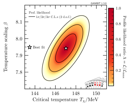
The two parameters $\beta$ and $T_{\chi}$ can then be constrained by using, e.g., the full lattice QCD results from Table S.7 in the supplementary material of Ref. 1606.07494 . We construct a likelihood function by performing a chi-squared fit to the $N=20$ data points,

$$\ln\left(\mathcal{L}\right)=-\frac{1}{2}\sum\limits_{i=1}^{N}\frac{(X-\hat{X}_{i})^{2}}{\sigma_{X_{i}}^{2}}\,,$$ (20)

where $X=\log_{10}\left[\chi(T\,|\,\beta,\,T_{\chi})/\chi(T=0)\right]$ is the logarithm of the normalised topological susceptibility, and $\hat{X}_{i}$ and $\sigma_{X_{i}}^{2}$ are its value and uncertainty for the $i$th data point. In Fig. 2, we show the two-dimensional profile likelihood for $\beta$ and $T_{\chi}$. These parameters show a clear correlation. This is expected, as a higher transition temperature implies a steeper slope in the temperature-dependent branch of the axion mass (corresponding to larger $\beta$) in order to maintain a good fit to the shape of $m_{a}(T)$, as determined by lattice QCD. We provide the best-fit values in Table 2.

We note that the fit to our functional form for the QCD axion mass (17) captures the temperature dependence established by lattice QCD well everywhere except in the region around $T=T_{\chi}$. This is because (17) is not smooth there and the overall fit is poor ($\chi^{2}=55.7$ for 18 d.o.f., which corresponds to a $p$-value of about $10^{-5}$). However, the disagreement stems only from a narrow temperature range, and has no impact on any of our results. Excluding the only data point in that region improves the fit to an acceptable level ($\chi^{2}=21.6$ for 17 degrees of freedom, which corresponds to a $p$-value of about 0.2).

We also replace the axion-electron coupling with the model-dependent factor $C_{aee}$

$$g_{aee}=\frac{m_{e}}{f_{a}}\;C_{aee}\,,$$ (21)

and the axion-photon coupling with the model-dependent ratio of the electromagnetic and colour anomalies $E/N$

$$g_{a\gamma\gamma}=\frac{\alpha_{\text{EM}}}{2\pi f_{a}}\left(\frac{E}{N}-\widetilde{C}_{a\gamma\gamma}\right)\,,$$ (22)

where $\widetilde{C}_{a\gamma\gamma}$ is the model-independent contribution from axion-pion mixing. We use the value obtained in Ref. 1511.02867 for $\widetilde{C}_{a\gamma\gamma}$ and include it as a simple nuisance likelihood,

$$\ln\left(\mathcal{L}\right)=-\frac{1}{2}\frac{(X-\hat{X})^{2}}{\sigma_{X}^{2}}\,,$$ (23)

with $X=\widetilde{C}_{a\gamma\gamma}$ and $\hat{X}$ and $\sigma_{X}$ again the most likely value and its uncertainty (see Table 2).

Finally, we want to emphasise some subtle considerations about the coupling strengths of the QCD axion model. The possible ratios $E/N$ are rational numbers arising from group theoretical considerations. In this study, we sample over $E/N$ as if it were a continuous parameter, as the possible rational numbers that it can take on are quite densely spaced along the real line, at least over the range of values that we consider. The sometimes so-called “classical axion window” considers a canonical, small and somewhat arbitrarily-defined range of couplings for the prototypical axion models Kaplan:1985dv ; hep-ph/9506295 ; hep-ph/9802220 ; PDG17 , arising from only quite a small range in $E/N$. It has recently been pointed out that the range of choices can, indeed, be extended to include more possibilities 1610.07593 ; 1705.05370 ; 1709.06085 ; 1712.04940 . To assess the whole range of various axion models, we use the minimum and maximum values for $E/N$ from Table IV in Ref. 1705.05370 , so that $E/N\in[-4/3,\,524/3]$. These values arise from a systematic study of DFSZ- and KSVZ-type axion models, where the additional heavy quarks in KSVZ-type models have cosmologically safe lifetimes and do not introduce Landau poles below the Planck scale. Furthermore, in DFSZ-type models, the number of Higgs doublets may go up to the maximum of nine.

Note that (22) implies the possibility of having $g_{a\gamma\gamma}<0$ within the valid range for $E/N$. Note however that all the likelihood functions that we use in this paper only depend on the absolute value of $g_{a\gamma\gamma}$. We therefore plot only $|g_{a\gamma\gamma}|$ in our results, even though we do scan over parameter values that lead to negative couplings in the range $-3.25\mathrel{\hbox to0.0pt{\lower 4.0pt\hbox{$\sim$}\hss}\raise 1.0pt\hbox{$<$}}E/N-\widetilde{C}_{a\gamma\gamma}\leq 0$.

3.2.1 KSVZ models

The archetypical axion model is the KSVZ model 1979_kim_ksvz ; 1980_shifman_ksvz , where the SM is supplemented by one or more electrically neutral, heavy quarks. In our implementation, the KSVZAxion is a child model of the QCDAxion, where the anomaly ratio, $E/N$, is a free parameter. In these models, axions have no tree-level interactions with fermions. However, there is a loop-induced coupling to electrons due to the axion-photon interaction, which – in the absence of a leading order contribution – must be taken into account 1985_srednicki_axioneft :

$$g_{aee}\approx\frac{3\alpha_{\text{EM}}^{2}}{2\pi}\left[\frac{E}{N}\ln\left(\frac{f_{a}}{m_{e}}\right)-\widetilde{C}_{a\gamma\gamma}\ln\left(\frac{\tilde{\Lambda}}{m_{e}}\right)\right]\frac{m_{e}}{f_{a}}\,,$$ (24)

where $\tilde{\Lambda}\sim$1\text{\,}\mathrm{GeV}$$ is the QCD confinement scale. Several previous works have used this expression with $\tilde{\Lambda}=$1\text{\,}\mathrm{GeV}$$ 1307.1488 ; 1708.02111 , even though this quantity is not uniquely defined. We too assume $\tilde{\Lambda}=$1\text{\,}\mathrm{GeV}$$, relying on the fact that any deviations enter only logarithmically. Although the anomaly ratio in the original KSVZ model was $E/N=0$ 1979_kim_ksvz ; 1980_shifman_ksvz , other assignments are possible. As in Ref. 1708.02111 , we will consider four different KSVZAxion models: $E/N=0,\,2/3,\,5/3,$ and $8/3$.

3.2.2 DFSZ models

In contrast to the KSVZ model, DFSZ models are obtained by adding an additional Higgs doublet to the SM 1980_zhitnitsky_dfsz ; 1981_dine_dfsz . This results in direct axion-electron interactions. One can define two manifestations of this model, often called DFSZAxion-I and DFSZAxion-II. The couplings in these two models are given by

$$\begin{array}[]{lll}C_{aee}=\sin^{2}(\beta^{\prime})\left/3\right.,\quad\phantom{.}&E/N=8/3\quad\phantom{.}&(\textsf{DFSZAxion-I})\\ C_{aee}=\left[1-\sin^{2}(\beta^{\prime})\right]\left/3\right.,\quad\phantom{.}&E/N=2/3\quad\phantom{.}&(\textsf{DFSZAxion-II})\end{array}$$ (27)

where $\tan(\beta^{\prime})$ is the ratio of the two Higgs vacuum expectation values 1985_srednicki_axioneft . Perturbative unitary requires $0.28<\tan(\beta^{\prime})<140$. It is therefore convenient to replace the parameter $C_{aee}$ in the QCDAxion model by $\tan(\beta^{\prime})$.

3.3 ALP models with constant mass

As a template model for ALPs that arise as pseudo-Nabu-Goldstone bosons but do not have a temperature-dependent mass, we define the ConstantMassALP model. This is mainly for convenience in studies where we want to parametrically explore the coupling space whilst keeping the inverse dependence on $f_{a}$, but are not interested in a temperature-dependent mass.

For ConstantMassALP models, $T_{\chi}$ is irrelevant because $\beta=0$, reducing the total number of parameters to five. Similar to QCDAxion models, we replace the ALP mass with a pseudo-Nambu-Goldstone scale $\Lambda$ and introduce dimensionless coupling constants $C_{a\gamma\gamma}$ and $C_{aee}$, consistent with the other models:

$$m_{a,0}=\frac{\Lambda^{2}}{f_{a}}\,,\qquad g_{a\gamma\gamma}=\frac{\alpha_{\text{EM}}}{2\pi f_{a}}\;C_{a\gamma\gamma}\,,\qquad g_{aee}=\frac{m_{e}}{f_{a}}\;C_{aee}\,.$$ (28)

4 Observables, experiments and likelihoods

Table 3: Overview of the likelihood functions that we employ in this paper (in the order they are discussed).

Likelihood/Observable	Comments	References
QCD nuisance parameters	Table 2	1511.02867 ; 1606.07494 ; Sec. 3.2
ALPS final limits	vacuum and argon data	1004.1313 ; Sec. 4.1
CAST 2007	vacuum data, CCD (2004)	hep-ex/0702006 ; Sec. 4.2.1 & Appendix A
CAST 2017	vacuum data, all detectors	1705.02290 ; Sec. 4.2.2 & Appendix A
RBF		based on DePanfilis:1987dk ; Wuensch:1989sa ; Sec. 4.3.1
UF		based on Hagmann:1990tj ; Sec. 4.3.2
ADMX 1998 – 2009		based on astro-ph/9801286 ; Asztalos:2001tf ; astro-ph/0310042 ; astro-ph/0603108 ; 0910.5914 ; Sec 4.3.3
ADMX 2018		based on 1804.05750 ; Sec. 4.3.4
DM relic density	built-in calculator; Sec. 4.4 and Appendix B	limits Planck15cosmo
H.E.S.S.	axion-photon conversion in galactic cluster magnetic fields	based on 1311.3148 ; Sec. 4.5.1
Supernova limits	axion-photon conversion in magnetic fields of the Milky Way	based on 1410.3747 ; Sec. 4.5.2
$R$ parameter		1406.6053 ; 1512.08108 ; Sec. 4.5.3
Stellar cooling hints (optional likelihood)
White dwarf cooling hints	only considered in Sec. 5.5	1205.6180 ; 1211.3389 ; 1605.06458 ; 1605.07668 ; Sec. 4.5.4

Table 3 gives an overview of the observables and likelihood functions that we use in this paper. In what follows, we give details of the experimental data, computational methods and likelihood implementations that they employ.

4.1 Light-shining-through-wall experiments

Light-shining-through-wall (LSW) experiments shine laser light through a magnetic field onto an opaque material, and attempt to detect it on the other side. A photon may convert into an axion within the magnetic field before the material, pass through it as an axion, and convert back into a photon in the magnetic field on the other side VanBibber:1987rq ; Anselm:1986gz ; Anselm:1987vj . Examples of experiments based on this technique are ALPS 0905.4159 ; 1004.1313 and OSQAR 0712.3362 ; 1506.08082 .

The predicted number of photons on the opposite side of the wall to the laser source is

$$s=\epsilon_{\text{tot}}\;\pazocal{P}\left(\gamma\to a\to\gamma\right)\frac{P}{\omega_{\gamma}}\,t_{\text{obs}}\,,$$ (29)

where $\epsilon_{\mathrm{tot}}$ is the detector efficiency, $P$ is the laser power, $\omega_{\gamma}$ the laser energy, and $t_{\text{obs}}$ the observation period. $\pazocal{P}\left(\gamma\to a\to\gamma\right)$ is the probability of a photon converting into an axion and back, in an appropriately aligned magnetic field of length $L$ and strength $B$. It is given by $\pazocal{P}\left(\gamma\to a\to\gamma\right)=\pazocal{P}^{2}\left(\gamma\to a\right)$ with 1004.1313

$$\pazocal{P}\left(\gamma\to a\right)=\pazocal{P}\left(a\to\gamma\right)=\left(\frac{g_{a\gamma\gamma}BL}{2}\right)^{2}\,\mathrm{sinc}^{2}\left(\frac{M^{2}L}{2\omega_{\gamma}}\right)\,,$$ (30)

where $M^{2}\equiv m_{a}^{2}/2+\omega_{\gamma}^{2}(n-1)$, $\mathrm{sinc}(x)\equiv\sin(x)/x$, $m_{a}$ is the axion mass, $\omega_{\gamma}$ is the photon energy, and $n$ is the refractive index of the medium in the experimental setup ($n=1$ for vacuum).

Our LSW likelihood is based on the final results of the ALPS-I experiment, using data for both evacuated and gas-filled magnets 1004.1313 . The ALPS Collaboration took data in “frames” of $t_{\text{f}}=$1\text{\,}\mathrm{h}$$ each, binning physical pixels of the detector into $3\times 3$-pixel blocks. ALPs refer to these simply as “pixels” of area $$42\text{\,}\mathrm{\SIUnitSymbolMicro m}$\times$42\text{\,}\mathrm{\SIUnitSymbolMicro m}$$. The collaboration searched their data frames for cosmic rays and signatures of other systematics, over a wide region around the single pixel where most of the laser light would fall in the absence of a wall, referred to as the “signal pixel”.

ALPS adjusted the raw ADU values (electron counts) of the signal pixel in an attempt to account for the average background in surrounding pixels. These reduced ADU (ADUred) values are obtained by subtracting the average ADU values across all pixels in the region surrounding the signal pixel, from the ADU value of the signal pixel. Doing this for every frame where the laser was on (“signal frames”) and off (“background frames”), ALPS constructed histograms of ADUred values for both signal and background. By fitting Gaussian functions to these histograms, they were able to estimate $\hat{b}$ and $\sigma_{b}$, the expected value and standard deviation of ADUred for the background, as well as $\hat{o}$ and $\sigma_{o}$, the equivalent quantities for signal frames. An example and more details can be found in Fig. 2 of Ref. 1004.1313 (see also Ref. 0905.4159 ).

From (29), the expected signal $s$ from photon-axion-photon production per frame of ALPS-I data (with $B=$4.98\text{\,}\mathrm{T}$$, $L=$4.2\text{\,}\mathrm{m}$$, and $\omega_{\gamma}=$2.33\text{\,}\mathrm{eV}$$) is

$$s\simeq$12.1$\;\epsilon_{\text{tot}}\;\left(\frac{P}{$1096\text{\,}\mathrm{W}$}\right)\left[\frac{g_{a\gamma\gamma}}{${10}^{-7}\text{\,}\mathrm{G}\mathrm{eV}^{-1}$}\;\mathrm{sinc}\left(\frac{M^{2}L}{2\omega_{\gamma}}\right)\right]^{4}\,.$$ (31)

Figure 3: Validation of our implementation of ALPS result for limits on the axion-photon coupling. We show the 90%, 95% and 99% C.L.s compared to the envelope of their strongest vacuum or gas results. The difference between our likelihood and the limit published by ALPS arises mostly due to the fact that we combine both likelihoods, rather than taking the envelope.

Apart from fluctuations in the experimental performance $\epsilon_{\mathrm{tot}}$, which amounts to an uncertainty of $\Delta\epsilon_{\text{tot}}/\epsilon_{\text{tot}}\approx 6\%$, the experimental parameters are known to sufficient precision to be fixed to their reference values. We incorporate the uncertainty on $\epsilon_{\mathrm{tot}}$ into the estimate of the signal prediction, $\sigma_{s}=s\Delta\epsilon_{\text{tot}}/\epsilon_{\text{tot}}$. As a result of the ADU reduction procedure, the measured signal and background estimators are non-integer numbers. We test the signal-plus-background hypothesis with a Gaussian likelihood:

$$\ln\left(\mathcal{L}_{i}\right)=-\frac{1}{2}\frac{\left[s_{i}-\left(\hat{o}_{i}-\hat{b}_{i}\right)\right]^{2}}{\sigma_{s,i\phantom{b}}^{2}+\sigma_{\hat{o}-\hat{b},i}^{2}}\,.$$ (32)

We add together the log-likelihoods for data sets $i=1$ to $3$, where two data sets (five and six frames compared to 122 and 47 background frames, respectively) consist of vacuum data and one data set (eight frames compared to 155 background frames) consists of argon gas data.

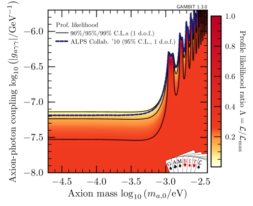
We show the resulting exclusion limits in Fig. 3 and compare with the envelope of the strongest vacuum or argon gas limits in Ref. 1004.1313 . The differences between the published results and our implementation are due to fact that we combine the likelihoods instead of just adopting the more constraining of the two, and also because the authors of Ref. 1004.1313 used the Feldman-Cousins method physics/9711021 , assuming Gaussianity and physical signals $s>0$. Considering the vacuum data alone, the method of Ref. physics/9711021 gives a slightly stronger limit than our log-likelihood ratio method ($6.5\text{\times}{10}^{-8}\text{\,}\mathrm{G}\mathrm{eV}^{-1}$ at 90% confidence limit (C.L.) in the low mass limit, as compared to $6.9\text{\times}{10}^{-8}\text{\,}\mathrm{G}\mathrm{eV}^{-1}$ in our implementation). By combining the vacuum and argon likelihoods however, our final limit is somewhat stronger: $g_{a\gamma\gamma}<$ $5.8\text{\times}{10}^{-8}\text{\,}\mathrm{G}\mathrm{eV}^{-1}$ at 90% C.L. at low masses.

4.2 Helioscopes

Axion helioscopes attempt to detect axions produced by interactions in the Sun by observing the solar disc with a “telescope” consisting of a long magnet contained in an opaque casing 1983_Sikivie ; 1985_Sikivie ; 1989_Bibber . Solar-produced axions would pass through the casing, convert into photons in the field of the magnet, and be observed in a detector behind the magnet.

Multiple processes in the Sun can produce axions: resonant production in the oscillating electric field of the solar plasma, non-resonant production in solar magnetic fields, and emission from the interaction of electrons with photons, nuclei or one another. The predicted axion-induced photon flux at Earth therefore depends on the assumed solar model, and on the couplings of the axion to both photons and electrons (see e.g. 1310.0823, ).

The dominant process for axion-photon interactions is Primakoff production 10.1103/PhysRev.81.899 ; 10.1103/PhysRev.152.1295 , where photons are resonantly converted into axions in the presence of an atomic nucleus. The rate at which axions of energy $E$ can be produced in a plasma from photons of the same energy is given by Raffelt:1985nk ; Raffelt:1987np

$$\Gamma_{\gamma\to a}=g_{a\gamma\gamma}^{2}\;\frac{\kappa_{s}^{2}T}{32\pi}\left[\left(1+\frac{\kappa_{\text{s}}^{2}}{4E^{2}}\right)\;\ln\left(1+\frac{4E}{\kappa_{\text{s}}^{2}}\right)-1\right]\,.$$ (33)

Here, the inverse screening length is given in the Debye-Hückel approximation by

$$\kappa_{\text{s}}^{2}=\frac{4\pi\alpha_{\text{EM}}}{T}\left(n_{e}+\sum_{j}Z_{j}^{2}n_{j}\right)\,,$$ (34)

with $n_{e}$ denoting the electron number density, and $n_{j}$ and $Z_{j}$ representing the number density and charge, respectively, of the $j$th nucleus. Note that the number densities and temperature, and hence the conversion rate, vary with the radial position $r$. Using the expression for the axion-photon conversion probability (30), the differential photon flux at the detector is hep-ex/0702006

$$\frac{\mathrm{d}\Phi(E)}{\mathrm{d}E} =2\pi\,\pazocal{P}\left(a\to\gamma\right)\,\int_{0}^{r_{s}}\!r\;\varphi_{\gamma\to a}(E,\,r)\,\mathrm{d}r\,,$$ (35)

$$\text{where}\quad\varphi_{\gamma\to a}(E,\,r) =\frac{R_{\odot}^{3}}{2\pi^{3}D_{\odot}^{2}}\int_{r}^{1}\!\frac{\rho}{\sqrt{\rho^{2}-r^{2}}}\;\frac{E\sqrt{E^{2}-\omega_{\text{pl}}^{2}(\rho)}}{\mathrm{e}^{E/T(\rho)}-1}\;\Gamma_{\gamma\to a}(E,\,\rho)\,\mathrm{d}\rho\,,$$ (36)

with $\rho$ a dimensionless radial co-ordinate in the Sun, and $r$ a dimensionless radial co-ordinate on the solar disc on the sky. The quantity $D_{\odot}$ is the (average) Sun-Earth distance, which we take to be one astronomical unit, and $\omega_{\text{pl}}^{2}(\rho)=4\pi\alpha_{\text{EM}}n_{e}(\rho)/m_{e}$ is the plasma frequency calculated from the electron number density $n_{e}(\rho)$ and electron mass $m_{e}$. The upper limit of outer integral, $r_{s}$, controls how much of the inner part of the image of the solar disc on the detector is included in the analysis. This need not always be 1, as the signal-to-noise ratio can be maximised by introducing a cut-off $r_{s}<1$ (see e.g. hep-ex/0702006, ).

The contribution to the solar axion flux from axion-electron interactions can be taken into account by including the additional interaction rate $\Gamma_{e\to a}(E,\,\rho)$ in (36). However, these contributions are not so straightforward to calculate from first principles. This is due to narrow free-bound transition lines Dimopoulos:1986kc ; Dimopoulos:1986mi ; 0807.3279 ; 1007.1833 , axion bremsstrahlung Zhitnitsky:1979cn ; Krauss:1984gm ; Raffelt:1985nk and Compton scattering Mikaelian:1978jg ; Fukugita:1982ep ; Fukugita:1982gn . To include these contributions in our signal prediction, we use tabulated data for the axion-electron spectrum provided in Ref. 1310.0823 .

The spectrum in Ref. 1310.0823 was computed with the 2009 iteration of the AGSS09met solar model 0909.2668 , which is based on photospheric abundances for non-refractory species and meteoritic abundances for refractory elements AGSS . The AGSS09met model is thus the default solar model in GAMBIT, and the one that we use throughout the rest of this paper. We however make use of its latest iteration 1611.09867 in preference to the earlier version wherever possible, such as when computing the axion flux from axion-photon interactions. In the limit of small axion mass, the predicted flux from axion-photon interations deviates by no more than 4.4% between solar models, with the greatest difference ocurring between the GS98 10.1023/A:1005161325181 ; 1611.09867 and most recent AGSS09met models 1611.09867 .

Full details of our integration routines for the axion-photon and axion-electron contributions, as well as the options available for the inclusion of solar models for axion physics in GAMBIT, can be found in Appendix A.

4.2.1 CAST results 2007

The first of our two CAST likelihoods is based on the CCD results published in 2007 hep-ex/0702006 (CCD detector data from the 2004 vacuum run in Table 1 of Ref. hep-ex/0702006 ). The other data in Ref. hep-ex/0702006 are less constraining; including them only improves the upper limit by 1% hep-ex/0702006 . We therefore do not provide separate likelihoods for the other runs.

Although the 2007 CAST analysis was based on the solar model of Ref. astro-ph/0402114 , and a follow-up analysis 1302.6283 on axion-electron interactions was based on a different model TurckChieze:2001ye , here we use the AGSS09met model of Ref. 1611.09867 . For both the axion-photon and axion-electron interactions, we integrate the total flux over all 20 energy bins (from $0.86.8\text{\,}\mathrm{keV}$), taking into account the observation time, effective area, and detector efficiency (see Appendix A). In this case $r_{s}\approx 0.23$ for the axion-photon contribution. As we use the interpolated spectrum for the axion-electron contribution (calculated for $r_{s}=1$), we can only rescale the resulting flux by an overall factor in order to estimate the flux inside $r_{s}=0.23$. We take this number to be 0.826, assuming the findings from the axion-photon interaction also apply in the axion-electron case hep-ex/0702006 .

Figure 4: Validation of our implementation of limits arising from the 2007 CAST data hep-ex/0702006 , including the 2013 re-interpretation in terms of axion-electron couplings 1302.6283 . Left: Exclusion limits for the axion-photon coupling hep-ex/0702006 . Right: Exclusion limits for the product of axion-photon and axion-electron coupling, assuming that axion-electron interactions dominate the axion production inside the Sun. We only make this assumption here to compare our implementation to Ref. 1302.6283 .

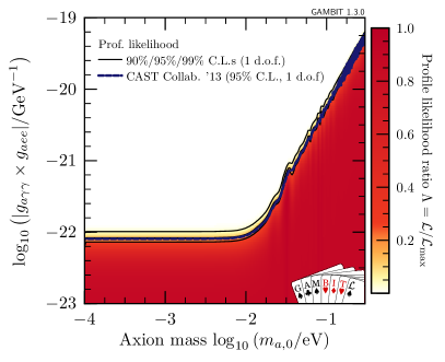
Our implementation follows the CAST analysis hep-ex/0702006 ; 1302.6283 , using a Poisson likelihood in each of the 20 energy bins

$$\ln\left(\mathcal{L}\right)=\sum\limits_{i=1}^{20}o_{i}\ln\left(s_{i}+b_{i}\right)-\ln\left(o_{i}!\right)-(s_{i}+b_{i})\,,$$ (37)

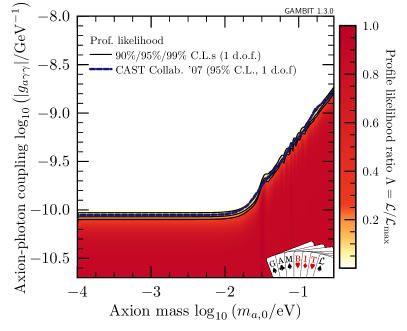
where $o_{i}$, $s_{i}$ and $b_{i}$ are respectively the observed number of photons, the number of expected signal photons, and the expected number of background photons based on observations away from the Sun, in the $i$th energy bin. In total, 26 photons were observed in the detector during data-taking compared to 30.9 expected background events. The resulting exclusion limits can be found in Fig. 4.

4.2.2 CAST results 2017

Our implementation of the latest CAST results 1705.02290 is analogous to that of the 2007 results, using the signal and expected background counts, exposure and detector efficiencies for the 2017 data.

To calculate the signal predictions, we integrate the axion-photon and axion-electron fluxes over each of the 10 energy bins from $27\text{\,}\mathrm{keV}$, and then scale the predictions by the effective exposure for each of the ten datasets in Ref. 1705.02290 .

Figure 5: Validation of our implementation of the 2017 CAST limits 1705.02290 . Differences are mainly due to our simplified implementation of the likelihood function, which does not employ event-level information.

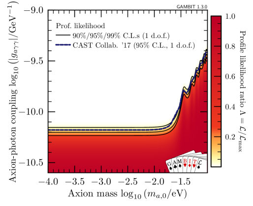
The exclusion limits presented in Ref. 1705.02290 are based on an unbinned likelihood. Here, we treat each energy bin in each of the ten datasets as a separate counting experiment, combining them into a binned Poisson likelihood

$$\ln\left(\mathcal{L}\right)=\sum\limits_{j=1}^{12}\sum\limits_{i=1}^{10}o_{i}^{(j)}\ln\left(s_{i}^{(j)}+b_{i}^{(j)}\right)+\ln\left(o_{i}^{(j)}!\right)-(s_{i}^{(j)}+b_{i}^{(j)})\,.$$ (38)

Here $o_{i}^{(j)}$, $s_{i}^{(j)}$ and $b_{i}^{(j)}$ are respectively the observed number of photons, the expected number of signal events and the expected number of background events in the $i$th energy bin of the $j$th experiment. In total, 226 photons were observed in the detector during data taking compared to 246.6 expected background events. Our slightly different choice of likelihood function to the original CAST analysis is significantly simpler, because it does not require event-level information – but it still reproduces the published exclusion limits rather well (see Fig. 5).

4.3 Haloscopes (cavity experiments)

Axion haloscopes are designed to detect DM axions by resonant axion-photon conversion inside a tunable cavity 1983_Sikivie ; 1985_Sikivie . Microwave cavities are the most sensitive axion experiments in existence, but only cover a small mass range compared to other techniques. The ability of haloscopes to detect axions therefore directly depends on their cosmological abundance, and to a lesser extent, their velocities in the Galactic halo 2011_Hoskins . Here we consider only the case where axions are fully virialised within the halo.

The power expected to be converted from axions to photons in a cavity is 1983_Sikivie ; Krauss:1985ub ; 1985_Sikivie

$$P=g_{a\gamma\gamma}^{2}\,B_{0}^{2}\,C\,\frac{\rho_{a,\text{ local}}\,V}{m_{a,0}}\,Q\,\min\left(1,\frac{Q_{a}}{Q}\right)\,,$$ (39)

where $C$ is the form factor (a dimensionless integral over the $\mathbf{E}$- and $\mathbf{B}$-field configuration of the cavity), $B_{0}$ is magnetic field strength in the cavity, $V$ is its volume, and $Q$ and $Q_{a}$ are the quality factors of the cavity and axions, respectively. In this context, $Q$ describes the ratio of stored vs dissipated energy of the cavity, while $Q_{a}$ is proportional to the axion velocity dispersion (just as $Q$ effectively characterises the bandwidth of the cavity).

The signal prediction also depends on the local DM density in axions, which we obtain by rescaling the local DM density as

$$\rho_{a,\text{ local}}=\min\left(\frac{\Omega_{a}}{\Omega_{\text{DM}}},1\right)\,\rho_{\text{DM, local}}\,.$$ (40)

Obtaining exclusion limits from cavity experiments is often quite involved, generally requiring simulation of the selection procedure of the detector (e.g. Asztalos:2001tf, ). Without access to this information, we must approximate the underlying likelihood functions based on the publicly available limits and publications.

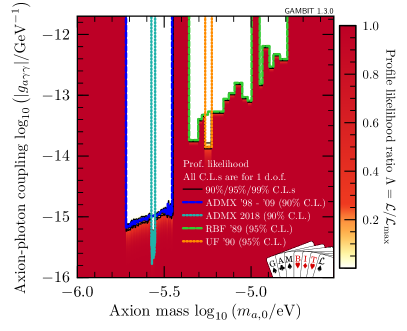
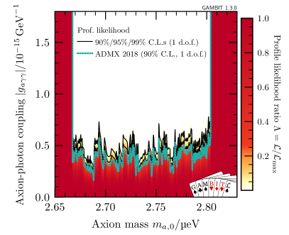
In the following, we describe our likelihoods for three different haloscope experiments. An overview of the resulting exclusion limits can be found in Fig. 6.

Figure 6: Left: Our implementation of haloscope likelihoods compared to the exclusion limits for the RBF DePanfilis:1987dk ; Wuensch:1989sa , UF Hagmann:1990tj and ADMX astro-ph/9801286 ; astro-ph/0104200 ; Asztalos:2001tf ; astro-ph/0310042 ; astro-ph/0603108 ; 0910.5914 ; 1105.4203 ; 1804.05750 experiments. Right: Magnified details of the latest ADMX results 1804.05750 .

4.3.1 RBF results

The Rochester-Brookhaven-Fermi (RBF) collaboration performed a search for axions using several cavities DePanfilis:1987dk ; Wuensch:1989sa . Table I, Eq. (26) and Fig. 14 in Ref. Wuensch:1989sa provide useful information for approximating their results.

By (39), the axion-induced power in a haloscope is proportional to $\rho_{a,\,\text{local}}^{\phantom{2}}\;g_{a\gamma\gamma}^{2}$, which we define as the “reduced signal”

$$s\equiv\rho_{a,\,\text{local}}^{\phantom{2}}\;g_{a\gamma\gamma}^{2}\,.$$ (41)

The remaining factors from (39) are effectively constant across all frequency/mass bins and detectors. The signal is expected to occur in a single frequency bin $i$, which satisfies $m_{a,0}\in[\omega_{i},\omega_{i+1})$. Using this definition, we adopt an ansatz for the likelihood function inspired by Eq. (26) of Ref. Wuensch:1989sa :

$$\ln\left(\mathcal{L}\right)=-\frac{1}{2}\Theta\left(s-a_{i}\right)\frac{(s-a_{i})^{2}}{b_{i}^{2}}\,.$$ (42)

Here $a_{i}$ is a threshold parameter, $b_{i}$ effectively corresponds to an expected standard deviation of the reduced signal, and $\Theta$ is the Heaviside step function. The threshold values $a_{i}$ arise because RBF manually inspected all candidate frequencies in their data over a certain significance level. The two parameters are related as $a_{i}=Nb_{i}$, where $N$ is the number of standard deviations required for manual inspection of a candidate signal.

Although Table I in Ref. Wuensch:1989sa would allow us to determine $b_{i}$, using the central frequency of the bin as well as the 95% C.L. on the coupling strength, the resulting bins are not quite identical to what is shown in Fig. 14 of the same paper. We therefore determine $a_{i}$ and $b_{i}$ for each frequency bin from the limits in Fig. 15 of that paper, assuming $N=4$ in all cases (cf. Table I in the same paper). This leads to limits in 14 bins ranging from $m_{a,0}=$4.4$$ to $10.1\text{\,}\mathrm{\SIUnitSymbolMicro eV}$ and from $m_{a,0}=$11.2$$ to $16.2\text{\,}\mathrm{\SIUnitSymbolMicro eV}$.

4.3.2 UF results

While the results from the University of Florida (UF) collaboration Hagmann:1990tj could be implemented in the same way as the RBF experiment, the published data do not allow us to infer the threshold parameter $a_{i}$ for the one mass bin. However, Eq. (6) in Ref. Hagmann:1990tj quotes the “noise power fluctuation”, which we use as a standard deviation $\sigma_{P}\approx$2.86\text{\times}{10}^{-22}\text{\,}\mathrm{W}$$ for the expected power $P$. We obtain the expected power for each axion model using the information provided in Ref. Hagmann:1990tj , and check that the quoted limit is comparable to the expected sensitivity (which we obtain by assuming that the observed data is equal to the background expectation). The corresponding likelihood function for the single bin from $m_{a,0}=$5.4$$ to $5.9\text{\,}\mathrm{\SIUnitSymbolMicro eV}$ and signal $s$ from (41) is given by

$$\ln\left(\mathcal{L}\right)=-\frac{1}{2}\left(\frac{P(s)}{\sigma_{P}}\right)^{2}\,.$$ (43)

4.3.3 ADMX results 1998–2009

The procedure used by the ADMX Collaboration for setting limits in the absence of a detection is highly customised for the experiment Asztalos:2001tf . Unfortunately, the necessary information for fully implementing their numerous results astro-ph/9801286 ; astro-ph/0104200 ; Asztalos:2001tf ; astro-ph/0310042 ; astro-ph/0603108 ; 0910.5914 is not available. Similar to the RBF likelihood, we therefore use the reduced signal (41) and the following ansatz for the likelihood:

$$\ln\left(\mathcal{L}\right)=-\frac{1}{2}\Theta\left(s/s_{i}-a\right)\frac{(s/s_{i}-a)^{2}}{b^{2}}\,.$$ (44)

Here $s_{i}$ is the known limit in the $i$th frequency/mass bin, and $a$ and $b$ are free parameters that have to be determined by a fit to published exclusion curves. We do this using the exclusion limits at three confidence levels published in Ref. astro-ph/9801286 , and by assuming that the shape of the likelihood function is representative of the shape in all other ADMX bins over the range from $m_{a,0}=$1.90$$ to $3.65\text{\,}\mathrm{\SIUnitSymbolMicro eV}$. Doing so results in $a=0.0131$ and $b=0.455$.

4.3.4 ADMX results 2018

In their recent publication, the ADMX collaboration increased the sensitivity of their setup, which is now able to rule out some DFSZ-type models 1804.05750 in the range $2.66\leq m_{a,0}\leq$2.81\text{\,}\mathrm{\SIUnitSymbolMicro eV}$$. We approximate the likelihood of this result using the 90% C.L. limits in Fig. 4 of Ref. 1804.05750 , for the Maxwell-Boltzmann velocity distribution (consistent with the model of the halo velocity distribution that we assume for analysing the results of other searches).

Because the experimental setup changed compared to the previous runs, we do not employ the shape parameters from Sec. 4.3.3 for the 2018 dataset. Instead, as with the UF experiment we assume that ADMX saw no signal events, approximating the 2018 likelihood as

$$\ln\left(\mathcal{L}\right)=-\frac{1}{2}\frac{s^{2}}{\sigma_{\text{eff}}^{2}(m_{a,0},\,s)}\,.$$ (45)

Here, the effective standard deviation is given by $\sigma_{\text{eff}}^{2}=\sigma_{\text{stat}}^{2}(m_{a,0})+\sigma_{\text{sys}}^{2}(s)$. We infer the statistical contribution $\sigma_{\text{stat}}$ by setting the log-likelihood at the observed values of the limits in Fig. 4 of Ref. 1804.05750 to that corresponding to a 90% C.L. for one degree of freedom. We read off $\sigma_{\text{stat}}$ at 194 different masses, and interpolate between them linearly for intermediate mass values (ignoring the narrow region from $2.73022.7307\text{\,}\mathrm{\SIUnitSymbolMicro eV}$ where the ADMX limits do not apply, due to radio interference 1804.05750 ). We add the systematic uncertainty of $13\%$ of the signal prediction (quoted in Ref. 1804.05750 ) in quadrature with the statistical uncertainty.

4.4 Dark matter relic density

Figure 7: Left: Realignment energy density in QCD axions today as a function of mass and initial misalignment angle (fixing $\beta$, $T_{\chi}$, and $\Lambda_{\chi}$ to their best-fit values for comparison). To guide the eye, we have included dotted and dashed lines to indicate where axions make up certain fractions of the DM relic density. Right: Band of $m_{a,0}$-$\theta_{\text{i}}$ combinations (from Diver) to get the correct DM density (including $\beta$, $T_{\chi}$, and $\Lambda_{\chi}$ as nuisance parameters). We show the results of Ref. 1606.07494 for comparison and also include the hypothetical case of a “temperature-independent QCD axion” (with $\Lambda_{\chi}$ as a nuisance parameter, but $\beta=0$ and $T_{\chi}$ irrelevant) as an example.

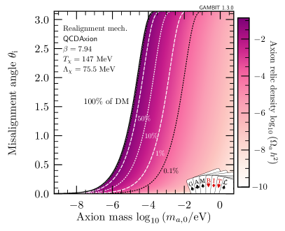
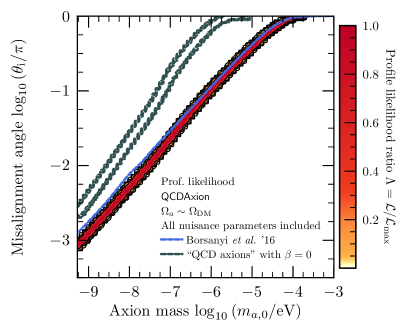
The realignment mechanism gives an axion contribution to the observed cold DM relic density. We solve (9) numerically as a function of temperature to obtain $\Omega_{a}$, the fraction of the critical energy density in axions today; details can be found in Appendix B. The resulting energy densities for the QCDAxion are shown in Fig. 7, similar to the presentation in other works (0903.4377, , e.g.). We reiterate that in this paper, we do not consider other contributions to the relic density than vacuum realignment.

The relic density of DM is very well constrained by the most recent Planck analysis Planck15cosmo . We employ a Gaussian likelihood with the central value and standard deviation from Planck15cosmo ($\Omega_{\text{DM}}h^{2}=0.1188$, $\sigma_{\mathrm{exp}}=0.0010$), combining the experimental uncertainty in quadrature with a further 5% theory uncertainty, $\sigma_{\mathrm{theo}}=0.05\,\Omega_{a}h^{2}$, to give

$$\ln\left(\mathcal{L}\right)=-\frac{1}{2}\frac{\left(\Omega_{a}h^{2}-\Omega_{\text{DM}}h^{2}\right)^{2}}{\sigma_{\text{exp}}^{2}+\sigma_{\text{theo}}^{2}}\,.$$ (46)

GAMBIT offers two options for this likelihood: a detection or an upper limit. These allow us to demand either that axions are responsible for all DM, or only a fraction. For the upper limit, we simply set $\ln\left(\mathcal{L}\right)=0$ for $\Omega_{a}<\Omega_{\text{DM}}$ in (46). Except where we state otherwise, we show results based on the upper limit option.

4.5 Astrophysical probes

Astrophysical systems can provide significant additional constraints on axions, especially the axion-electron and axion-neutron couplings, which are not well constrained by other probes. Due to their weak interactions with matter, axions can efficiently transport energy across large distances in free space, or through stellar matter, thereby influencing stellar structure and evolution.

Intriguingly, a number of astrophysical systems appear to exhibit an unexplained mechanism of energy transport, which might be due to ALPs: white dwarfs display apparently anomalous cooling rates (Sec. 4.5.4) or deviations in the shape of their luminosity function 1406.7712 ; 1805.00135 and highly-energetic gamma rays seem to experience significantly less attenuation through intergalactic space than might be expected 0707.4312 ; 0712.2825 ; 1001.0972 ; 1106.1132 ; 1201.4711 ; 1302.1208 . Unfortunately, the systematic uncertainties associated with these potential hints of new physics are quite difficult to quantify. Nonetheless, if the observations and associated theoretical uncertainties turn out to be robust, ALPs can indeed explain the observed deviations from expectation.

4.5.1 Distortions of gamma-ray spectra

Axions can be generated in galactic or intergalactic magnetic fields, distorting or dimming the spectra of distant sources Raffelt:1987im ; hep-ph/0111311 ; hep-ph/0204216 ; 0704.3044 . Several studies have investigated the effects of ALPs on otherwise featureless spectra 0706.3203 ; 0707.2695 ; 0708.1144 ; 0911.0015 ; 1205.6428 ; 1305.2114 , and used the resulting limits to constrain ALP properties 1311.3148 ; 1603.06978 ; 1801.01646 ; 1801.08813 ; 1802.08420 .

The probability of photon-axion conversion in a domain of size $\ell$ filled with a suitably aligned magnetic field $B_{\text{eff}}$ and plasma with electron number density $n_{e}$ is given by Raffelt:1987im ; 0911.0015

$$p_{1}(E)\equiv\pazocal{P}\left(\gamma\to a\right)=\frac{1}{1+\left(\frac{E_{\text{crit}}}{E}\right)^{2}}\;\sin^{2}\left(\frac{1}{2}\,g_{a\gamma\gamma}\,B_{\text{eff}}\,\ell\;\sqrt{1+\left(\frac{E_{\text{crit}}}{E}\right)^{2}}\right)\,,$$ (47)

where $\omega_{\text{pl}}$ and $E_{\text{crit}}$ are the plasma frequency and critical energy, respectively:

$$\omega_{\text{pl}}^{2}=\frac{4\pi\alpha_{\text{EM}}\,n_{e}}{m_{e}}\,,\quad E_{\text{crit}}=\frac{1}{2}\frac{\left|m_{a}^{2}-\omega_{\text{pl}}^{2}\right|}{g_{a\gamma\gamma}\,B_{\text{eff}}}\,.$$ (48)

The quantity $E_{\text{crit}}$ describes the energy scale at which photons will efficiently convert into axions in the extragalactic magnetic field domains. In the absence of dust or any other photon absorber, after traversing $N$ such domains of size $\ell$, the remaining fraction of photons is hep-ph/0111311 ; hep-ph/0204216 ; astro-ph/0607415 ; 0911.0015

$$\pazocal{P}\left(\gamma\to\gamma\right)=\frac{2}{3}+\frac{1}{3}\mathrm{e}^{-\frac{3Np_{1}}{2}}\,.$$ (49)

Equations (47) and (49) reveal that we do not expect to see any effect due to axions for $E\ll E_{\text{crit}}$, because $p_{1}\simeq 0$. For a given photon energy $E$, this happens for large axion masses $m_{a}$ and small axion-photon couplings $g_{a\gamma\gamma}$.

For $E\gg E_{\text{crit}}$, on the other hand, conversion is very efficient, but the observed spectrum would simply decrease by a constant factor over the entire energy range. In this case it is also not possible to test the axion hypothesis: the expected spectral normalisation of any source is not well constrained and it therefore has to be a free fitting parameter in the analysis.

Figure 8: Our implementation of the H.E.S.S. exclusion limits from gamma-ray spectral distortions of PKS 2155-304, based on the limits quoted in Figs 6 and 7 of Ref. 1311.3148 . Full details of the likelihood construction can be found in Appendix C.

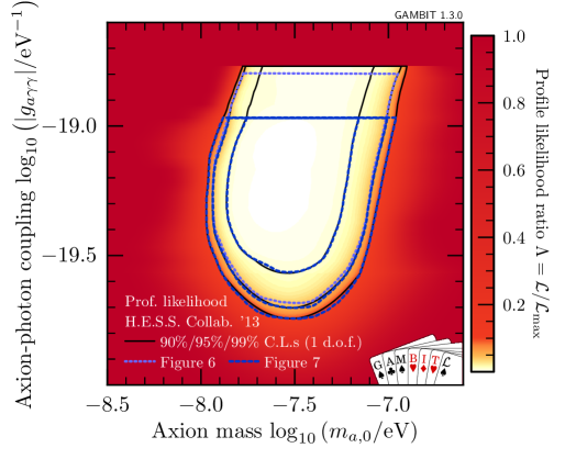
It is only possible to constrain models where the critical energy lies within the spectral window of the instrument, such that one end of the spectrum is suppressed, but the other is not 1205.6428 ; 1305.2114 . Limits from the distortion of gamma-ray spectra are therefore strongest at axion masses that lead to threshold energies similar to the photon energies observed by the experiment. This explains the characteristic shape of the limits (in particular why this method is not sensitive to axion masses below a certain value; see Fig. 8).

The H.E.S.S. Collaboration applied this technique to the spectrum of the active galactic nucleus PKS 2155-304, using data obtained with their Cherenkov telescope array 1311.3148 . Unfortunately, their signal prediction requires Monte Carlo simulation of magnetic field realisations, which are no longer available.

We therefore approximate their likelihood function for the galactic cluster magnetic field using Figs 6 and 7 of Ref. 1311.3148 , based on a scheme that we describe in detail in Appendix C. The main idea is to use common interpolation methods inside the published exclusion contours, and to extrapolate to likelihood values outside the known contours using a method that mimics the shape of the known iso-likelihood contours and preserves the mathematical properties of the likelihood. Our approximation procedure is of course somewhat arbitrary. The advantages of our scheme are that it exactly reproduces the known exclusion curves by construction, and that the general likelihood function is well-behaved. The obvious downsides are that we can neither guarantee that the likelihood in the outermost and innermost regions are completely accurate, nor can we extend it to larger couplings than the values shown in Fig. 7 of Ref. 1311.3148 .

4.5.2 Supernova 1987A

Supernovae are excellent particle laboratories. Supernova 1987A (SN1987A) provides significant constraints on axion parameters, based on the neutrino burst duration Ellis:1987pk ; Raffelt:1987yt ; Turner:1987by ; Mayle:1987as and axion-photon interaction in magnetic fields external to the supernova astro-ph/9605197 ; astro-ph/9606028 .

Our likelihood for SN1987A is based on the results from Ref. 1410.3747 . The authors of that study derived limits based on the absence of a coincident gamma-ray burst from SN1987A, which should have been observed by instruments on board of the Solar Maximum Mission Chupp:1989kx if axions were produced in the explosion and converted to gamma rays in the Galactic magnetic field.

The gamma-ray spectrum of photons with energy $E$ expected at Earth per unit time from axions produced in SN1987A is

$$\frac{\mathrm{d}\Phi_{a\to\gamma}}{\mathrm{d}E}=\frac{1}{4\pi d^{2}}\;\frac{\mathrm{d}\dot{N}}{\mathrm{d}E}\;\pazocal{P}\left(a\to\gamma\right)\,,$$ (50)

where $d$ is the distance to the supernova, $\pazocal{P}\left(a\to\gamma\right)$ is the conversion probability (47), $N$ is the number of axions created in the supernova and $\mathrm{d}\dot{N}/\mathrm{d}E$ is the axion spectrum at the source, as predicted from a supernova model. To obtain the measured photon fluence at Earth (gamma rays per unit area during the observation), $\mathcal{F}_{a\to\gamma}$, equation (50) has to be integrated over the energy range and time duration of the observation, while modelling the transport of the axions through the Galactic magnetic field.

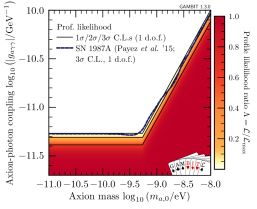
From Fig. 6 in Ref. 1410.3747 , we can see that the photon fluence at Earth for a given axion-photon coupling becomes constant below a certain mass scale $m_{\ast}$ and rapidly decreases for bigger masses. This is not surprising, given that most axion experiments lose sensitivity at large masses due to the loss of coherence in axion-photon conversion. We therefore make the following ansatz for the fluence,

$$\mathcal{F}_{a\to\gamma}=F\,\left(\frac{g_{a\gamma\gamma}}{$5.3\text{\times}{10}^{-10}\text{\,}{\mathrm{GeV}}^{-1}$}\right)^{4}\,\begin{cases}\hfil 1&\text{for }m_{a}\leq m_{\ast}\\ \left(\frac{m_{\ast}}{m_{a}}\right)^{b}&\text{for }m_{a}>m_{\ast}\,,\end{cases}$$ (51)

where $F\approx$0.57\text{\times}{10}^{-12}\text{\,}\mathrm{c}\mathrm{m}^{-2}$$ is the fluence for small axion masses at the reference value of $g_{a\gamma\gamma}\approx$5.3\text{\times}{10}^{-10}\text{\,}\mathrm{G}\mathrm{eV}^{-1}$$; we obtain this value by integrating Eq. (2.11) in Ref. 1410.3747 .

We determine the best-fit values for $m_{\ast}$ and the exponent $b$ from the higher-mass region ($m_{a,0}>$6.0\text{\times}{10}^{-10}\text{\,}\mathrm{eV}$$) via a least-squares fit to the fluence contour in Fig. 6 of Ref. 1410.3747 , giving $\hat{m}_{\ast}\approx$5.43\text{\times}{10}^{-10}\text{\,}\mathrm{eV}$$ and $\hat{b}\approx 4.02$. The value of $\hat{b}$ that we obtain can be qualitatively understood by examining the axion-photon conversion probability given in (47), which can be written as $\pazocal{P}\left(\gamma\to a\right)=\sin^{2}(c\sqrt{x})/x$, where $c=g_{a\gamma\gamma}B_{\text{eff}}\ell/2$ does not depend on $m_{a}$. For axions masses $m_{a}\gg\omega_{\text{pl}}$ (with $\omega_{\text{pl}}\sim$4\text{\times}{10}^{-12}\text{\,}\mathrm{eV}$$), we have $x\propto m_{a}^{4}$ and, since the oscillatory part is washed out by the turbulent magnetic fields, the conversion probability is effectively suppressed by a factor of $m_{a}^{4}$.

Figure 9: Our implementation of SN1987A limits compared to Ref. 1410.3747 (dashed line).

The likelihood for $s=\mathcal{F}_{a\to\gamma}$ in the absence of a photon signal with background fluctuations $\sigma_{\mathcal{F}}^{2}$ is then given by

$$\ln\left(\mathcal{L}\right)=-\frac{1}{2}\frac{s^{2}}{\sigma_{\mathcal{F}}^{2}}\,.$$ (52)

Fig. 9 shows how the limits obtained from our approximation compare to the original reference.

4.5.3 Horizontal Branch stars and R parameter

Weakly-interacting particles can influence stellar evolution by providing an additional energy loss mechanism, cooling stars over the course of their evolution Sato:1975vy ; Raffelt:1990yz ; book_raffelt_laboratories . The so-called $R$ parameter, $R=N_{\text{HB}}/N_{\text{RGB}}$, is the ratio between the number of Horizontal Branch (HB) stars, $N_{\text{HB}}$, and upper Red Giant Branch (RGB) stars, $N_{\text{RGB}}$, in Galactic globular clusters. Its value depends on the relative time that stars spend on each branch, which is sensitive to the details of stellar evolution and cooling. Axions are expected to be produced in the cores of both types of stars, but would remove heat more efficiently from the cores of HB stars, reducing the time that they spend on the HB and leading to a reduction in $R$.

Based on a weighted average of a selection of cluster count observations astro-ph/0403600 , the observed value is $R_{\text{obs}}=1.39\pm 0.03$ 1406.6053 . The dependence of the predicted value of the $R$ parameter on the properties of axions can be approximated as 1512.08108 ; 1983A&A…128…94B ; Raffelt:1989xu ; 1311.1669 ; 1406.6053

$$R_{\text{pred}}\approx 7.33\,Y -0.422-0.0949\left(-4.68+\sqrt{21.9+21.1\,x_{a\gamma\gamma}}\right)$$

$$-0.00533\,x_{aee}^{2}-0.0387\left(-1.23-0.138\,x_{aee}^{1.5}+\sqrt{1.51+x_{aee}^{2}}\right)\,,$$ (53)

where $Y$ is the Helium abundance, $x_{a\gamma\gamma}\equiv g_{a\gamma\gamma}/${10}^{-10}\text{\,}\mathrm{G}\mathrm{eV}^{-1}$$ and $x_{aee}\equiv g_{aee}/${10}^{-13}$$. The equation above is valid only if axions are sufficiently light compared to the typical temperatures of the stellar interior, which are $T\sim${10}^{8}\text{\,}\mathrm{K}$\approx$10\text{\,}\mathrm{keV}$$ book_raffelt_laboratories , i.e. much higher than the axion masses we consider. Our $R$ parameter likelihood is then simply

$$\ln\left(\mathcal{L}\right)=-\frac{1}{2}\frac{\left(R_{\text{pred}}-R_{\text{obs}}\right)^{2}}{\sigma_{\text{pred}}^{2}+\sigma_{\text{obs}}^{2}}\,,$$ (54)

where $\sigma_{\mathrm{pred}}$ and $\sigma_{\mathrm{obs}}$ are the uncertainties of the predicted and observed values.

Figure 10: Comparison of our implemented $R$ parameter likelihood with the $1\sigma$ and $2\sigma$ contours (dashed and dotted blue lines) of Ref. 1512.08108 . Note that our adopted likelihood leads to limits only, whereas the results of Ref. 1512.08108 indicate an almost $2\sigma$ preference for signal (hence the presence of $1\sigma$ upper and lower limits in the results that we plot from Ref. 1512.08108 ). The difference is due to the updated He abundance that we employ here.

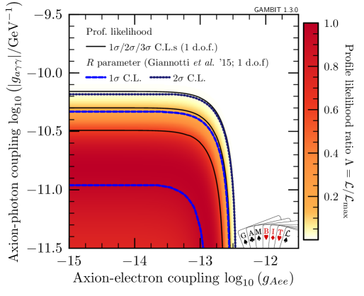
The authors of Ref. 1512.08108 adopted a Helium abundance of $Y=0.255\pm 0.002$ 1408.6953 , leading to a predicted value from standard (axion-free) stellar evolution calculations of $R_{\text{theo}}=1.45\pm 0.01$, almost $2\sigma$ higher than the observed value. We adopt the updated value for such low-metallicity environments of $Y=0.2515\pm 0.0017$ 1503.08146 , leading to $R_{\text{theo}}=1.42\pm 0.01$, entirely consistent with the observed $R$ parameter. The effect of the uncertainty of $Y$ on $R_{\text{pred}}$ can be estimated according to (53), as $\sigma_{\text{pred}}=7.33\times 0.0017\approx 0.012$. A comparison to the exclusion curves in Ref. 1512.08108 can be found in Fig. 10.

4.5.4 White Dwarf cooling hints

White dwarfs (WDs) are a particularly interesting environment in which to study axion-electron interactions, due to their electron-degenerate cores Raffelt:1985nj ; Nakagawa:1987pga ; Nakagawa:1988rhp ; Isern:1992gia . Current observations can be interpreted as indicating a need for additional cooling in WDs compared to standard models. The coupling necessary to explain the cooling with axions has been estimated to be $g_{aee}\sim\pazocal{O}\left(${10}^{-13}$\right)$ 1512.08108 . A more recent analysis also considered these cooling hints in a global fitting framework 1708.02111 . Whilst the systematics of such analyses are still a matter of debate, and alternative explanations (whether involving BSM physics or not) are certainly still possible, it is intriguing to investigate the impact on axion global fits of including the WD cooling hints. Due to the speculative nature of theses hints, we will do so in a separate (alternative) analysis in Sec. 5.5, presented alongside our main global fits.

WDs typically pulsate, allowing the oscillation of their radii and luminosity to be used to probe their internal structure via astroseismology. The periods, $\Pi$, of their pulsations decrease with time, with a rate $X=\mathrm{d}\Pi/\mathrm{d}t$, which can be related to the energy loss in the system.

Table 4: Overview of available cooling hints for WD variables of spectral types DA and DB. We list the couplings allowed at $2\sigma$ confidence (whether limits or intervals). The numerical values necessary for constructing the corresponding likelihoods were kindly provided by A. H. Córsico and T. Battich. In the case of R548, we have two more data points compared to what is shown in Fig. 1 of Ref. 1211.3389 .

Object	Type	Mode		$2\sigma$ C.L.	References
		$k$	$\ell$	$g_{aee}/${10}^{-13}$$
G117-B15A	DA variable	2	1	$\left[3.4,\,6.0\right]$	Fig. 5 1205.6180 ; hep-ph/9310304 ; astro-ph/0104103 ; 0711.2041 ; 0806.2807
R548	DA variable	2	1	$\left[0.30,\,6.8\right]$	Fig. 1 1211.3389 ; 0711.2041
L19-2	DA variable	2	1	$<5.1$	Fig. 5 1605.06458
PG 1351+489	DB variable	11	1	$<3.6$	Fig. 5 1605.07668

Refs 1205.6180 ; 1211.3389 ; 1605.06458 ; 1605.07668 simulated the evolution of WDs with and without axions, predicting the period decrease $\mathrm{d}\Pi/\mathrm{d}t$ in each case. For our predictions of WD cooling rates, we interpolate these results and their stated uncertainties, using natural splines. The specific figures and objects from those papers that our implementation is based on are listed in Table 4. Note that the plots in Refs 1205.6180 ; 1211.3389 ; 1605.06458 ; 1605.07668 show the quantity $m_{a,0}\cos^{2}(\beta^{\prime})$ which, for the DFSZAxion-I axion model they consider, is proportional to the more fundamental parameters $C_{aee}$ or $g_{aee}$ (cf. Sec. 3.2.2). For values of the axion-electron coupling larger than considered in the simulations (i.e. $g_{aee}/${10}^{-13}$>5.6$ or $8.4$), we assign the likelihood corresponding to the largest simulated coupling. This is a conservative assumption, as the disagreement between prediction and observation will in reality only worsen as the coupling increases further (until the WDs become opaque to axions – but this would occur at couplings well beyond what we consider).

Figure 11: Overview of the WD likelihoods available in GAMBIT. We show the separate likelihoods (left) as well as the combined result (right). To guide the eye, horizontal dashed lines indicate the confidence levels. Note that, taken at face value, the combined constraints have the potential to be significant evidence for an additional cooling channel in WDs.

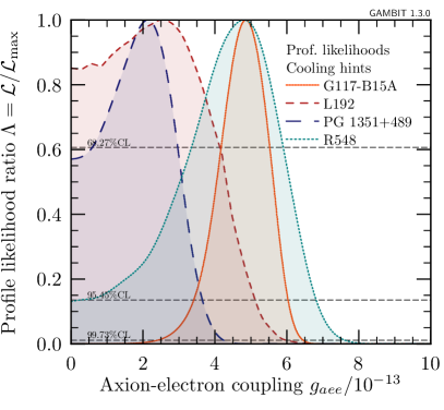
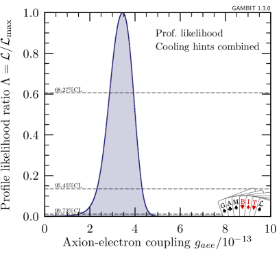
For each WD listed in Table 4, we use a simple Gaussian likelihood function for the observed ($X_{\text{obs},i}$) and theoretically-expected ($X_{\text{pred},i}$) period decrease, such that our total WD cooling likelihood is

$$\ln\left(\mathcal{L}\right)=-\frac{1}{2}\sum_{i=1}^{4}\frac{\left(X_{\text{pred},i}-X_{\text{obs},i}\right)^{2}}{\sigma_{\text{pred},i}^{2}+\sigma_{\text{obs,}i}^{2}}\,,$$ (55)

where, again, the predictions and corresponding uncertainties $\sigma_{\text{pred},i}$ are taken from the respective figures in the references listed in Table 4 and interpolated via natural splines. The resulting individual and combined likelihoods can be found in Fig. 11.

We emphasise that the interpretation of WD cooling is subject to a number of assumptions and caveats. Statistical and systematic uncertainties associated with the inputs and algorithms of stellar models were considered by the authors of Refs 1205.6180 ; 1211.3389 ; 1605.06458 ; 1605.07668 , but a number of other potential issues remain. These include theoretical modelling of the transition from the main sequence to the WD phase, and the accuracy of the observed period decrease of PG 1351+489. Despite these problems, and in contrast to Ref. 1708.02111 , we include the PG 1351+489 system in our discussion. The authors of Ref. 1708.02111 exclude this object due to its similarity to R548, and the uncertainties associated with R548 being “more conservative”. However, the different estimated uncertainties in these two systems are in fact due to a real physical effect, namely the difference in the influence of trapped vs non-trapped oscillation modes in the two systems. While the latter might give rise to concerns regarding the understanding of different modes (cf. Table 4), we do not conclude that the arguments in favour of excluding PG 1351+489 are strong enough to do so.

5 Results and discussion

In this section, we present the central findings from our global fits of various axion models, identifying the most promising regions in parameter space and comparing the various models. We present frequentist and Bayesian results side-by-side, after discussing our choice of priors for the model parameters. Unless stated otherwise, all C.L.s and C.R.s (Bayesian credible regions) are $1\sigma/2\sigma/3\sigma$ ($68.27\%/95.45\%/99.73\%$), and all C.L.s are two-sided for two degrees of freedom (d.o.f.). Secs. 5.2–5.4 do not include WD cooling hints; these are the subject of a dedicated analysis in Sec. 5.5.

5.1 Sampling algorithms and settings

We use the differential evolution sampler Diver ScannerBit to sample the composite likelihood function and T-Walk ScannerBit to sample the posterior distributions. We employ MultiNest 0704.3704 ; 0809.3437 ; 1306.2144 primarily to compute Bayesian evidences.

We use the sampler settings established in an earlier study by the GAMBIT Collaboration as starting points ScannerBit . For Diver, we generally use a population size (NP) of $2\text{\times}{10}^{4}$ and a tolerance (convthresh) of ${10}^{-4}$, and turn off the lambdajDE optimisation, preferring to use regular jDE for its slightly less aggressive optimisation. In addition to combining samples from various runs, where necessary to resolve fine-tuned regions we increase NP to $3\text{\times}{10}^{4}$ or $5\text{\times}{10}^{4}$ and/or reduce convthresh to ${10}^{-5}$. For T-Walk, we use the default settings for 340 or 544 MPI processes, until reaching a tolerance ($\texttt{sqrtR}-1$) of $0.01$ or $0.005$. All initialisation YAML files that we use in this study are available on Zenodo Zenodo_axions ; the exact scans for which we use the different settings can be ascertained by examining the input files. Because we use MultiNest primarily for estimating Bayesian evidences, we set the sampling efficiency (efr) to 0.3, as recommend for this task 0809.3437 , and use $2\text{\times}{10}^{4}$ live points (nlive) with a tolerance (tol) of ${10}^{-4}$.

5.2 General ALP models

Starting at the top of the model hierarchy (see Fig. 1), we first consider the GeneralALP model. This is a phenomenological model; parameter combinations in this model need not correspond to physical models, as their couplings do not depend on the inverse of $f_{a}$. The main purpose of the GeneralALP is to provide a straightforward, universal connection to observables and to compare to results in the literature.

Table 5: Parameter ranges and scaling for GeneralALP models.

Model	Parameter range/value		Scale
GeneralALP	$f_{a}\,[$\mathrm{GeV}$]$	$[${10}^{6}$,\,${10}^{16}$]$	log
	$m_{a,0}\,[$\mathrm{eV}$]$	$[${10}^{-10}$,\,$1$]$	log
	$g_{a\gamma\gamma}\,[$\mathrm{G}\mathrm{eV}^{-1}$]$	$[${10}^{-16}$,\,${10}^{-8}$]$	log
	$g_{aee}$	$[${10}^{-22}$,\,${10}^{-10}$]$	log
	$\theta_{\text{i}}$	$[$-3.141\,59$,\,$3.141\,59$]$	flat
	$\beta$	$[$0$,\,$16$]$	flat
	$T_{\chi}\,[$\mathrm{MeV}$]$	$[${10}^{-2}$,\,${10}^{6}$]$	log
Local DM density	$\rho_{0}\,[$\mathrm{G}\mathrm{eV}\mathrm{/}\mathrm{c}\mathrm{m}^{3}$]$	$[$0.2$,\,$0.8$]$	flat

Parameter ranges.

The parameter ranges and scales that we use for GeneralALP models are given in Table 5. Because the axion potential is periodic, all normalised field values are equivalent to a value in the interval $(-\pi,\,\pi]$. For $g_{a\gamma\gamma}$, $g_{aee}$, and $m_{a,0}$, there is no obvious range to choose; we adopt parameter ranges encompassing values informed by previous studies and phenomenology. Recall that $g_{a\gamma\gamma}$ could be negative but the likelihood functions in the present work only depend its absolute value. We therefore scan only over positive values of $g_{a\gamma\gamma}$, but label plots with $|g_{a\gamma\gamma}|$, to make it explicit that the results are equally valid for the corresponding negative values. For the local DM density $\rho_{0}$, we adopt the same range as in earlier GAMBIT studies MSSM ; SSDM ; CMSSM ; SSDM2 (and implement the same likelihood function).

The appropriateness of different ranges on $f_{a}$, $\beta$, and $T_{\chi}$ depends on the fundamental properties of the symmetries and scales of the underlying ALP model. Although there are theoretical arguments for the existence of ALPs from e.g. string theory hep-th/0605206 ; 1201.5902 , they do not provide any quantitative guidance. Apart from the likely case that our calculations become meaningless for $f_{a}\mathrel{\hbox to0.0pt{\lower 4.0pt\hbox{$\sim$}\hss}\raise 1.0pt\hbox{$>$}}m_{\text{Pl}}$, we can only impose $\beta>0$, as the axion mass should become smaller as the underlying symmetry is restored at higher temperatures. The ranges in Table 5 are therefore an attempt to include a variety of cases around the values known or preferred for the QCD axion.

We do not produce Bayesian results for the GeneralALP model, as no strong physical arguments exist for any particular choice of prior on most of its parameters. The only exception is the initial misalignment angle $\theta_{\text{i}}$, due to the causal structure of the early-Universe cosmology mentioned in Sec. 2.3.1.

Figure 12: Profile likelihood for GeneralALP models assuming ALPs to be all of dark matter. The constraints that dominate the exclusion contours are CAST, haloscopes (UF, RBF and ADMX), H.E.S.S., the $R$ parameter, and SN 1987A. We used Diver to sample the profile likelihood (interpolated density plot) and a root-finding algorithm with a local optimisation routine for profiling to determine the $2\sigma$ C.L. (dashed line). For comparison, we also show the band of QCD axion models that we consider in this paper (blue shaded region; cf. Sec. 5.3) and the discrete choices for $E/N$ that we use for the DFSZ- and KSVZ-type models (yellow lines; dealt with in detail in Secs. 5.4 and 5.5.2).

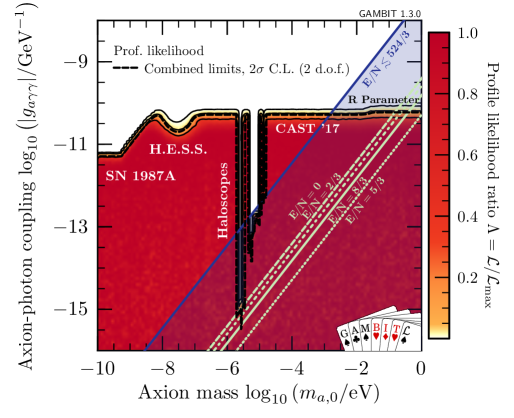
Frequentist results.

We first scan the GeneralALP model assuming ALPs to be all of DM. The resulting limits on the axion-photon coupling (Fig. 12) are comparable to summary plots elsewhere in the literature (e.g. PDG17, ). However, we would like to stress that unlike overplotted exclusion limits, the exclusion curve in Fig. 12 arises from a composite likelihood, and profiling takes into account uncertainties in the local DM density (the only relevant nuisance parameter here).

Figure 13: Profile likelihoods (from Diver) for GeneralALP models, assuming they provide all of the dark matter in the Universe. We show limits for the axion-photon and axion-electron couplings (left; essentially dominated by the $R$ parameter likelihood, cf. Fig. 10) and for the absolute value of the initial misalignment angle vs $f_{a}$ (right).

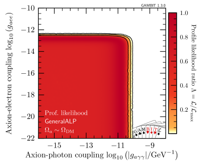
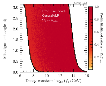
The left panel of Fig. 13 shows that the joint constraints on the two coupling parameters are essentially dictated by the constraint on the $R$ parameter (Fig. 10). As a consequence, the axion-electron equivalent of Fig. 12 would show that values of $g_{aee}\mathrel{\hbox to0.0pt{\lower 4.0pt\hbox{$\sim$}\hss}\raise 1.0pt\hbox{$>$}}\text{few}\times${10}^{-13}$$ are excluded across the entire mass range. The right panel of Fig. 13 shows the possible combinations of $f_{a}$ and $|\theta_{\text{i}}|$ that allow the GeneralALP to be all of DM. The extent and shape of this region is mostly due to the limited ranges of $m_{a,0}$, $\beta$, and $T_{\chi}$. The axion potential, and therefore the initial energy density in axions, is proportional to $f_{a}\,m_{a,0}$. The observed DM abundance can only be achieved if $f_{a}\,m_{a,0}$ is large enough, because $|\theta_{\text{i}}|<\pi$. On the other hand, the axion starts to oscillate when $H\sim m_{a}$ (Sec. 2.3.1). The associated temperature scale depends on $m_{a,0}$, $\beta$, and $T_{\chi}$ and sets the amount by which the axion energy density is red-shifted up to the present day. To obtain the correct abundance in axions today while e.g. going to lower values of $f_{a}$, the values of $m_{a,0}$, $\beta$, or $\theta_{\text{i}}$ must be increased or the value of $T_{\chi}$ decreased.

Figure 14: Profile likelihoods (from Diver) for specific GeneralALP models that constitute all of the dark matter in the Universe. We compare the allowed regions between QCD-like ALPs with $\beta=7.94$ and $T_{\chi}=$147\text{\,}\mathrm{MeV}$$ (density plot and black contours) and simpler GeneralALP models with $\beta=0$ (grey contours). Note that in the figure in the left panel, the region to the right of the grey contours is allowed for this model.

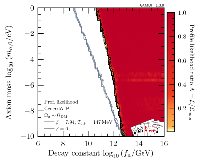
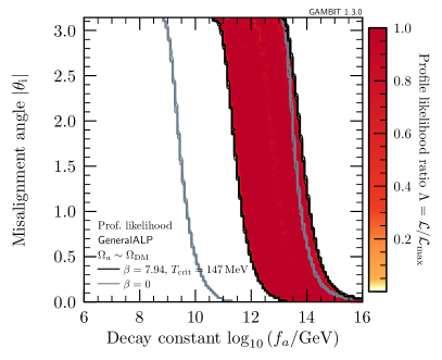
Within our selected parameter ranges, the profile likelihood does not identify preferred regions for $T_{\chi}$ and $\beta$. However, as Fig. 14 shows, different choices of $T_{\chi}$ and $\beta$ can lead to different behaviours in the profile likelihoods of other quantities. Due to the temperature dependence of the axion energy density (11). For example, in Fig. 14, we choose a generalised QCDAxion-like model (with $\beta=7.94$ and $T_{\chi}=$147\text{\,}\mathrm{MeV}$$) and compare it to a ConstantMassALP-like model ($\beta=0$). The different slope of the exclusion region boundary in the left panel of Fig. 14 is a consequence of how the energy density scales right after the axion field begins to oscillate. For the allowed range of values for $m_{a,0}$, the corresponding band of possible $f_{a}$ – given a value for the initial misalignment angle – is also different.

5.3 QCD axions

QCD axions are the most well-studied type of axions to date. Unlike in previous studies, here we take into account the uncertainties due to nuisance parameters (see Sec. 3.2) in every part of the analysis. We also consistently scale the local DM density in axions according to their cosmological abundance. This affects the limits on the axion-photon interaction from haloscope experiments such as ADMX, as the detector signal in (41) is proportional to $\rho_{a,\text{local}}^{\phantom{2}}\,g_{a\gamma\gamma}^{2}$. The limits on $g_{a\gamma\gamma}$ therefore scale with $1/\sqrt{\rho_{a,\,\text{local}}}$. We again cap the local axion abundance at 100% of the local DM abundance, and penalise models that predict too much DM via the Planck likelihood for $\Omega_{\text{DM}}h^{2}$ (Sec. 4.4).

Prior choices.

The priors that we apply to the QCDAxion parameters can be found in Table 6. This model imposes a number of relations between the phenomenological parameters of its parent GeneralALP model, which depend on nuisance parameters, i.e. quantities determined by simulations, theory or experiments, which are only known within an appreciable uncertainty. While we are generally not interested in inference on such parameters, their uncertainties can affect results for the actual parameters of interest. The additional nuisance parameters for QCDAxion models are $\widetilde{C}_{a\gamma\gamma}$, $\Lambda_{\chi}$, $\beta$, and $T_{\chi}$. For $\widetilde{C}_{a\gamma\gamma}$ and $\Lambda_{\chi}$, the nuisance likelihood is given by a 1D Gaussian for each parameter, whereas the likelihood for $\beta$ and $T_{\chi}$ takes into account correlations between the two parameters (Sec. 3.2). We choose flat priors from about $-5\sigma$ to $+5\sigma$ around the respective central values for all four nuisance parameters.

Table 6: Prior choices for QCDAxion models.

Model	Parameter range/value		Prior type
QCDAxion	$f_{a}\,[$\mathrm{GeV}$]$	$[${10}^{6}$,\,${10}^{16}$]$	log
	$\Lambda_{\chi}\,[$\mathrm{MeV}$]$	$[$73$,\,$78$]$	flat
	$\widetilde{C}_{a\gamma\gamma}$	$[$1.72$,\,$2.12$]$	flat
	$E/N$	$[$-1.333\,33$,\,$174.667$]$	flat
	$C_{aee}$	$[${10}^{-4}$,\,${10}^{4}$]$	log
	$\theta_{\text{i}}$	$[$-3.141\,59$,\,$3.141\,59$]$	flat
	$\beta$	$[$7.7$,\,$8.2$]$	flat
	$T_{\chi}\,[$\mathrm{MeV}$]$	$[$143$,\,$151$]$	flat
Local DM density	$\rho_{0}\,[$\mathrm{G}\mathrm{eV}\mathrm{/}\mathrm{c}\mathrm{m}^{3}$]$	$[$0.2$,\,$0.8$]$	flat

The range of values that we choose for the anomaly ratio, $E/N$, is inspired by the selection criteria and range established in phenomenological studies of axion models (cf. Sec. 3.2). While the different preferred models presented in Ref. 1705.05370 form a discrete set, we assume that there is a continuous band of possible axion models, spanning a range from the lowest ($E/N=-4/3$) to the highest ($E/N=524/3$) possible value of the anomaly ratio. Given that the number of possibilities grows very quickly if we allow for an arbitrary number of new heavy quarks in KSVZ-type models (where, however, $E/N\leq 170/3$), it is not inconceivable that such a band exists. We treat each value inside the band as equally probable before contact with data, employing a flat prior for $E/N$. Note that this necessarily encompasses negative values for $g_{a\gamma\gamma}$, as discussed in Sec. 3.1; whilst this does not impact our likelihoods (which depend only on $|g_{a\gamma\gamma}|$), it does imply an asymmetric effective prior on the two signs of $g_{a\gamma\gamma}$.

Assigning priors to $f_{a}$ and $C_{aee}$ is more difficult. For $f_{a}$, we choose a range that corresponds to our region of interest in mass: from the largest masses allowed by bounds on hot DM, to highly fine-tuned regions with very small masses and $f_{a}$ somewhat below the Planck scale. The logarithmic prior reflects our ignorance about the scale of new physics, given that the ability of the original QCD axion to solve the Strong CP problem does not depend on the value of $f_{a}$. We choose a generous range for $C_{aee}$, taking a logarithmic prior around values of order unity, which may be considered the most natural value for $C_{aee}$. Note that the lower end roughly corresponds to the minimum value that can be constrained by the $R$ parameter for the highest QCDAxion masses we consider. Values any lower will be effectively indistinguishable.

Our choice of priors on $\rho_{0}$ and $\theta_{\text{i}}$ follow the logic from the previous section on GeneralALP models. Because $\rho_{0}$ is rather well constrained by data, the choice of log or flat prior has little impact on the final results. For $\theta_{\text{i}}$, the causal structure of the early-Universe cosmology mentioned in Sec. 2.3.1 means that all values of the initial misalignment angle are equally likely, so a flat prior is most appropriate.

Frequentist results.

Figure 15: Profile likelihoods (from Diver) for QCDAxion models with upper limits (left) and matching condition (right) for the observed DM relic density. The upper and lower panels show the constraints on the anomaly ratio, $E/N$, and the absolute value of the initial misalignment angle, $|\theta_{\text{i}}|$, respectively.

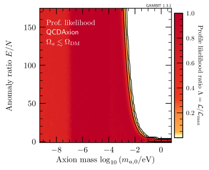
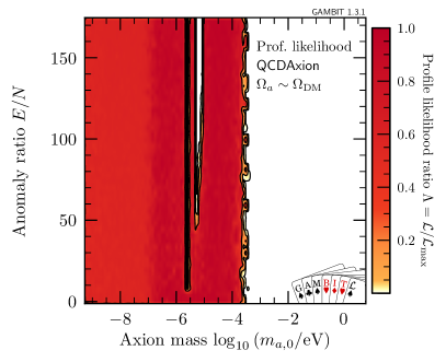
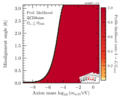
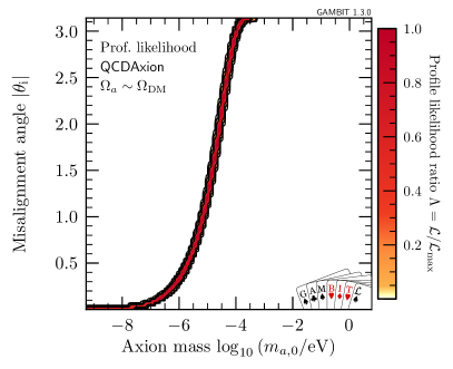
First, let us consider statistical inference on the axion coupling strengths. There are essentially only upper limits on the axion couplings or the associated model parameters. We begin by focusing on the axion-photon interactions, as determined by the anomaly ratio $E/N$, shown in the upper row of Fig. 15. In the left panel we impose the relic density constraint as an upper limit, while in the right panel we demand that axions be all of DM. A notable difference between these two assumptions is that haloscopes (UF, RBF and ADMX) only provide strong limits in the latter case.

If axions are not required to be all of DM, the high-mass (low-$f_{a}$) region is excluded by the $R$ parameter and CAST likelihoods (cf. Fig. 12) except at very low values of $E/N$. If axions constitute all of the DM in the Universe, these constraints are not relevant because the realignment mechanism cannot produce enough DM when $|\theta_{\text{i}}|\leq 3.14159$ and $m_{a,0}\mathrel{\hbox to0.0pt{\lower 4.0pt\hbox{$\sim$}\hss}\raise 1.0pt\hbox{$>$}}$1\text{\,}\mathrm{meV}$$ (cf. right panel of Fig. 7), so the high-mass region is excluded.

We also see slightly lower profile likelihood values for masses below about $0.1\text{\,}\mathrm{\SIUnitSymbolMicro eV}$. This is due to the role of the axion-electron coupling in the $R$ parameter likelihood: while our updated value for the helium abundance reduces the tension between theory and observations, there is still a slight preference for $g_{aee}\neq 0$. For small masses, however, the maximum allowed value for the axion-electron coupling, $C_{aee}\leq${10}^{4}$$, is still not large enough to satisfy this small preference.

In the bottom row of Fig. 15, we show the allowed values for the magnitude of the initial misalignment angle, with and without the assumption that axions constitute all of DM. Due to the influence of the various nuisance parameters and the relic density likelihood, the allowed region in the right panel is not simply a line, but a band of parameter combinations that reproduce the observed DM density within the allowed uncertainties. This panel also illustrates the well-known result that the initial misalignment angle needs to be fine-tuned, i.e. $\left|\theta_{\text{i}}\right|\ll 1$, for QCD axion masses of $m_{a,0}\mathrel{\hbox to0.0pt{\lower 4.0pt\hbox{$\sim$}\hss}\raise 1.0pt\hbox{$<$}}$0.1\text{\,}\mathrm{\SIUnitSymbolMicro eV}$$. We will investigate this issue in more detail below using a Bayesian analysis.

Bayesian results.

Breaking the PQ symmetry before inflation effectively results in a single, homogeneous value for the misalignment angle in the entire observable Universe. This gives a physical motivation for choosing a flat prior on $\theta_{\text{i}}$. Parameter regions in which $\theta_{\text{i}}$ must be very small to avoid axion overproduction are hence theoretically less appealing. In a Bayesian analysis, we can see and quantify these fine-tuning issues in the (marginalised) posterior distributions, which quantify the degree of belief in certain values of the parameters given data and prior information.

Figure 16: Marginalised posteriors (from T-Walk) for QCDAxion models with upper limits (left) and matching condition (right) for the observed DM relic density. The upper and lower panels show the constraints on the anomaly ratio, $E/N$, and the absolute value of the initial misalignment angle, $|\theta_{\text{i}}|$, respectively.

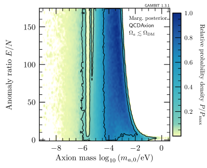
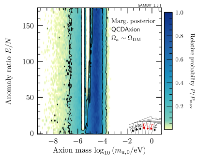
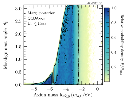
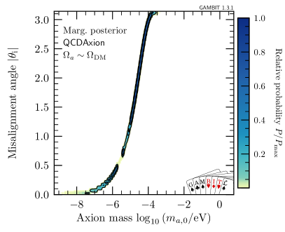
We show marginalised posteriors for the QCDAxion model in Fig. 16, once again without (left) and with (right) the requirement that QCD axions are all of DM. As a consequence of fine-tuning in $\theta_{\text{i}}$, the low-mass (high-$f_{a}$) region of the parameter space in Fig. 16 is disfavoured, even when taking the DM relic density as an upper limit only. This is because in the low-mass region, large absolute values of the initial misalignment angles have a small likelihood. An $\pazocal{O}(1)$ value for the magnitude of the initial misalignment angle is a priori more probable than finding a value close to zero, due to the flat prior. This conflict leads to fine-tuning becoming increasingly necessary as the axion mass decreases, which is penalised in the Bayesian analysis. Although such parameter combinations might still give valid solutions that evade all constraints, they are not as probable as others.

A similar logic applies to large axion-photon coupling, i.e. large $E/N$. Due to the fine-tuning in $E/N$ necessary to evade the helioscope and $R$ parameter constraints at large axion mass (cf. the corresponding profile likelihood in the top left panel of Fig. 15), the large-$m_{a,0}$ (low-$f_{a}$) region in the top left panel of Fig. 16 is disfavoured in the Bayesian posterior.

If we demand that axions explain all of DM, the consequences are even more dramatic. The most probable axion models are confined to the narrow band in $m_{a,0}$, visible in the upper right panel of Fig. 16. This mass range presents a feasible target for haloscope searches, and ADMX in particular is already beginning to cut into these models from the left (low-mass end). This also explains why the band of $m_{a,0}$-$\theta_{\text{i}}$ values in the bottom right panel of Fig. 16 is not continuous, but disrupted around two points. These correspond to the ADMX and RBF/UF haloscope searches, respectively. While the RBF and UF haloscopes cannot reach as far down into the coupling space as ADMX, they do still constrain a significant fraction of the coupling range.

Figure 17: Profile likelihoods (from Diver, left) and marginalised posteriors (from T-Walk, right) for the mass in QCDAxion models with upper limits (red shading) and matching condition (blue shading) for the DM relic density. The prior-dependence of the marginalised posteriors is investigated in Appendix D.

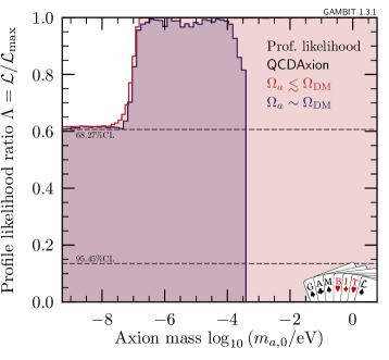
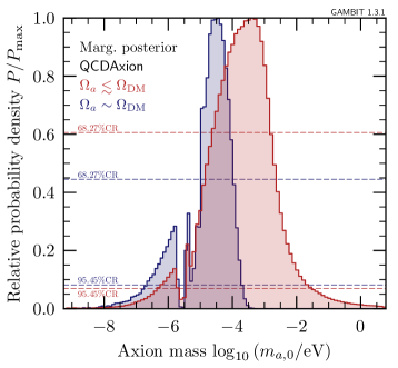
The fact that the Bayesian analysis singles out a well-defined range for the QCD axion mass becomes even more apparent in Fig. 17, where we compare one-dimensional profile likelihoods and marginalised posteriors for the axion mass. The frequentist approach does not yield a clear preference for any mass range, but the posterior distributions are strongly peaked around $m_{a,0}\sim$100\text{\,}\mathrm{\SIUnitSymbolMicro eV}$$. Clearly, such a result is not completely prior-independent, and we discuss the impact of adopting different priors in Appendix D. Nevertheless, it is appealing that a Bayesian analysis can identify a preferred region of $m_{a,0}$ which, intriguingly, falls into the range that can be covered by experimental searches. Indeed, the impact of ADMX and other haloscopes already manifests itself as dips in the right panel of Fig. 17.

The marginalised posterior in Fig. 17 allows us to infer a preferred QCDAxion mass range. When demanding that axions explain all of DM, we find that the 95% equal-tailed credible interval for the axion mass is $$0.10\text{\,}\mathrm{\SIUnitSymbolMicro eV}$\leq m_{a,0}\leq$0.16\text{\,}\mathrm{meV}$$; allowing them to constitute a fraction of DM, this becomes $$0.60\text{\,}\mathrm{\SIUnitSymbolMicro eV}$\leq m_{a,0}\leq$7.1\text{\,}\mathrm{meV}$$. These numbers have minimal dependence on the adopted prior for $E/N$, but a stronger dependence on the choice of priors for $C_{aee}$ and $f_{a}$ (Appendix D).

We also note that if the PQ symmetry is broken after inflation, the preferred axion mass range will generally shift to larger values due to averaging of the energy density and inclusion of topological defects (cf. Sec. 2.3). The lower bounds on $m_{a,0}$ that we quote can therefore be viewed as robust against changes of assumptions about inflation.

Figure 18: Profile likelihoods (from Diver, left) and marginalised posteriors (from T-Walk, right) for $\Omega_{a}h^{2}$ in QCDAxion models with upper limits (red shading) and matching condition (blue shading) for the DM relic density.

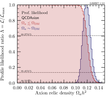
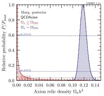
Finally, we also show the one-dimensional profile likelihoods and marginalised posteriors for the QCDAxion relic density in Fig. 18. Demanding that axions be all of the DM effectively dominates the outcome of this analysis. Using the DM relic density as an upper limit causes the profile likelihood to essentially follow the relic density likelihood function (left panel). In a Bayesian analysis, however, we immediately see that QCDAxions are not expected to generally provide all of the DM in the Universe, given our definition of the parameter space and priors. Imposing the DM relic density as an upper limit, the median axion relic density is $4.2\text{\times}{10}^{-3}$, or about 3.6% of the observed DM abundance. The 95% credibility equal-tailed preferred range is $$3.7\text{\times}{10}^{-6}$\leq\Omega_{a}h^{2}\leq$0.10$$, which corresponds to between about 0.003% and 84% of the cosmological density of DM. This demonstrates that in the pre-inflationary PQ symmetry-breaking scenario, although QCDAxions can provide a sizeable contribution to the DM density of the Universe, they probably do not contribute all of DM. Again, we stress that these statements are sensitive to the adopted prior on $C_{aee}$ and $f_{a}$ (Appendix D).

5.4 DFSZ- and KSVZ-type models

The DFSZ-type (DFSZAxion-I, DFSZAxion-II) and KSVZ-type (KSVZAxion) models differ from their parent model, the QCDAxion, in that they specify the axion-photon and axion-electron coupling strengths, or at least limit them to a well-defined range for a given axion mass. They are but a few of the many possible phenomenologically-inspired models, but they serve as interesting archetypes of their respective subclasses to compare with more general QCDAxion models.

Prior choices.

Table 7: Prior choices for DFSZAxion-I, DFSZAxion-II and KSVZAxion models. Note that the priors listed in the first section of the table apply to all three models.

Model	Parameter range/value		Prior type	Comments
	$f_{a}\,[$\mathrm{GeV}$]$	$[${10}^{6}$,\,${10}^{16}$]$	log	Applies to all
	$\Lambda_{\chi}\,[$\mathrm{MeV}$]$	$[$73$,\,$78$]$	flat	Applies to all
	$\widetilde{C}_{a\gamma\gamma}$	$[$1.72$,\,$2.12$]$	flat	Applies to all
	$\theta_{\text{i}}$	$[$-3.141\,59$,\,$3.141\,59$]$	flat	Applies to all
	$\beta$	$[$7.7$,\,$8.2$]$	flat	Applies to all
	$T_{\chi}\,[$\mathrm{MeV}$]$	$[$143$,\,$151$]$	flat	Applies to all
DFSZAxion-I	$E/N$	$8/3$	delta
	$\tan(\beta^{\prime})$	$[$0.28$,\,$140.0$]$	log
DFSZAxion-II	$E/N$	$2/3$	delta
	$\tan(\beta^{\prime})$	$[$0.28$,\,$140.0$]$	log
KSVZAxion	$E/N$	$0$, $2/3$, $5/3$, $8/3$	delta	Various discrete choices
Local DM density	$\rho_{0}\,[$\mathrm{G}\mathrm{eV}\mathrm{/}\mathrm{c}\mathrm{m}^{3}$]$	$[$0.2$,\,$0.8$]$	flat

Our prior choices for the DFSZ and KSVZ model can be found in Table 7. For most of them, the rationale is the same as for QCDAxions presented in Sec. 5.3. The only differences are in the parameters related to couplings. We fix $E/N$ to some typical values considered previously in the literature (e.g. 1708.02111, ). The range that we choose for $\tan(\beta^{\prime})$ in DFSZ-type models reflects the values allowed by perturbativity bounds 1301.0309 . Our choice of a log prior for $\tan(\beta^{\prime})$ reflects the assumption that each possible Higgs vacuum expectation value is equally likely; indeed, any sensible prior choice for this parameter should reflect the fact that the two Higgs doublets may be interchanged, and the prior should be invariant under inversion of the ratio of vacuum expectation values.

Frequentist results.

The DFSZ- and KSVZ-type models are essentially restrictions of the allowed QCD axion couplings. We therefore only expect to see qualitative differences in the results from the different models where the DFSZ and KSVZ interaction strengths cannot be tuned sufficiently to evade constraints from haloscopes (if axions make up all of DM) and the $R$ parameter.

Figure 19: Profile likelihood (from Diver) for the axion mass in the different DFSZ- and KSVZ-type models, imposing the DM relic density as an upper limit.

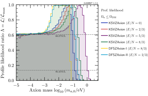
Figure 19 shows the profile likelihood constraints on various axion models, imposing the DM density as an upper limit. We can see that the upper limit on the axion mass depends on the value of $E/N$ in a given model (cf. Fig. 12), giving KSVZAxion models with $E/N=5/3$ the largest allowed parameter space out of all the models compared here. The different values for $E/N$ are also the reason for the different positions of the peaks in $m_{a,0}$; the slight preference for non-zero couplings in the $R$ parameter likelihood requires slightly different axion masses for different $E/N$.

Demanding that axions explain all of DM, Fig. 19 would change slightly. All models with $m_{a,0}\mathrel{\hbox to0.0pt{\lower 4.0pt\hbox{$\sim$}\hss}\raise 1.0pt\hbox{$>$}}$0.1\text{\,}\mathrm{meV}$$ would be ruled out (not being able to provide all of the DM through the realignment mechanism), and ADMX would partially constrain all models except those with $E/N=5/3$ (cf. Fig. 12).

Figure 20: Profile likelihood (from Diver) for KSVZAxion (left), DFSZAxion-I (right; blue contours), and DFSZAxion-II models (right; coloured region and black contours), compared to the profile likelihood for the QCDAxion model (grey lines). All results use the observed relic density of DM as an upper limit on the relic axion abundance.

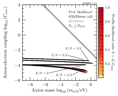
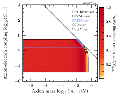
The relation between the DFSZ- and KSVZ-type models and their parent QCDAxion model determines their allowed axion-electron couplings. Figure 20 shows how the allowed parameter space in the $m_{a,0}$-$C_{aee}$ parameter plane of the QCDAxion model is constrained further by imposing additional relations between the different model parameters in the KSVZ- and DFSZ-type models.

This is most striking in the case of the KSVZ-type models, for which $C_{aee}$ is only induced at the loop level and depends directly on $m_{a,0}$ (24). Note that the ordering of the KSVZAxion regions is also non-monotonic in $E/N$ due to the difference term in (24). The finite sizes of the allowed parameter regions are simply a result of the nuisance parameters included in the relation between $C_{aee}$ and $m_{a,0}$. For DFSZ-type models, $C_{aee}$ depends on the additional parameter $\tan(\beta^{\prime})$, which makes it possible to accommodate a wide range of axion-electron couplings. However, the parameter space is also more constrained in this case, as very large values of $C_{aee}$ cannot be realised given other constraints on $\tan(\beta^{\prime})$. Also note that, due to the different coupling structure in DFSZAxion-I and DFSZAxion-II models (27), the same range for $\tan(\beta^{\prime})$ translates into a lower minimal value of $C_{aee}$ in DFSZAxion-II models than in DFSZAxion-I models. The resulting possible range for $C_{aee}$ in DFSZAxion-II models (and KSVZAxion models with $E/N=5/3$) also extends to slightly lower values than the prior box that we chose for QCDAxions.

Bayesian results.

We use the nested sampling package MultiNest to estimate the Bayesian evidences $\mathcal{Z}(\mathcal{M})$ for each model $\mathcal{M}$. From these we construct the Bayes factor Jeffreys:1939xee ; 10.2307/2291091 ; 10.2307/4356165

$$\mathcal{B}\equiv\frac{\mathcal{Z}(\mathcal{M}_{1})}{\mathcal{Z}(\mathcal{M}_{2})}\equiv\frac{\int\!\mathcal{L}\left(\text{data}\left|\right.\boldsymbol{\theta_{1}}\right)\mathcal{P}_{1}(\boldsymbol{\theta_{1}})\,\mathrm{d}\boldsymbol{\theta_{1}}}{\int\!\mathcal{L}\left(\text{data}\left|\right.\boldsymbol{\theta_{2}}\right)\mathcal{P}_{2}(\boldsymbol{\theta_{1}})\,\mathrm{d}\boldsymbol{\theta_{2}}}\,,$$ (56)

where $\mathcal{M}_{1}$ and $\mathcal{M}_{2}$ are the two models under investigation, $\boldsymbol{\theta_{1}}$ and $\boldsymbol{\theta_{2}}$ are their parameters, $\mathcal{P}_{1}$ and $\mathcal{P}_{2}$ are their priors and $\mathcal{L}$ is the likelihood. The Bayes factor is connected to the odds, i.e. the ratio of posterior probabilities, of the models being correct:

$$\frac{\mathcal{P}\left(\mathcal{M}_{1}\left|\text{data}\right.\right)}{\mathcal{P}\left(\mathcal{M}_{2}\left|\text{data}\right.\right)}=\mathcal{B}\;\frac{\mathcal{P}(\mathcal{M}_{1})}{\mathcal{P}(\mathcal{M}_{2})}\,.$$ (57)

In this paper, we assign equal prior probabilities to both models being correct, i.e. choose $\mathcal{P}(\mathcal{M}_{1})/\mathcal{P}(\mathcal{M}_{2})=1$, so the Bayes factor is the same as the posterior odds ratio.

Using MultiNest’s nested sampling (as opposed to importance nested sampling) estimates for evidences, we calculated the odds in favour of KSVZ- and DFSZ-type axion models over the QCDAxion model. In terms of the commonly used scale for Bayes factors Jeffreys:1939xee ; 10.2307/2291091 , we find that there is generally no noticeable evidence for or against any of these models, which would require an odds ratio of more than 3:1 (or less than 1:3).

Imposing the relic DM density as an upper limit, the odds in favour of any KSVZ- or DFSZ-type axion models, compared to QCDAxions, are 2:1. If we demand that axions constitute all of DM, the odds reduce to 1:1.

The outcome of the model comparison is not surprising, as we have not included any positive evidence for axions at this stage. We will discuss in the following section how these conclusions change when including WD cooling hints.

5.5 Cooling hints

Observables related to stellar cooling offer a unique opportunity to constrain the axion parameter space. If future observations confirm the need for additional cooling channels to explain the observed decreases in WD pulsation periods, we may be able to use WDs to measure the axion mass and coupling strengths. In this section we add the likelihoods related to the WD cooling hints to our analysis, emphasising once again the caveats and difficulties associated with assigning uncertainties to the model predictions (cf. Sec. 4.5.4). Here our prior choices for each model are the same as in the preceding sections. A detailed numerical comparison of our results to previous works 1512.08108 ; 1708.02111 is not meaningful due to differences in the choice of WD likelihood function, but the findings are qualitatively similar.

5.5.1 QCD axions

Previous studies have mostly considered the phenomenological couplings $g_{a\gamma\gamma}$ and $g_{aee}$ or specific QCD axion models with fixed $E/N$. Here, we investigate which parts of the broader QCDAxion parameter space can explain the cooling hints.

Frequentist results.

Figure 21: Profile likelihoods (from Diver) for QCDAxion models with upper limits (left) and matching condition (right) for the observed DM relic density and including cooling hints. The upper and lower panels show the constraints on the anomaly ratio, $E/N$, and for the absolute value of the initial misalignment angle, $|\theta_{\text{i}}|$, respectively.

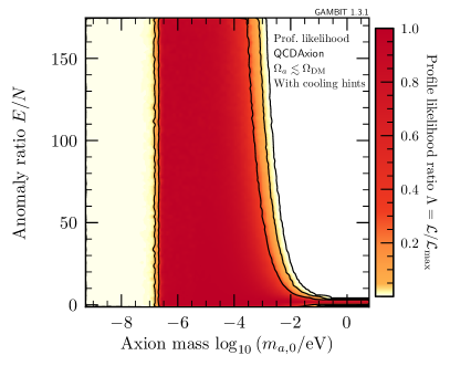
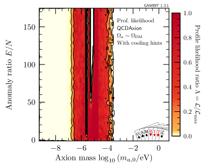
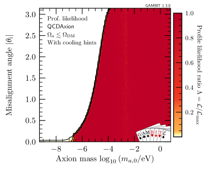
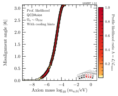
Figure 21 is the cooling-hint equivalent of Fig. 15, summarising the allowed anomaly ratio and magnitude of the initial misalignment angle. The only notable difference is at $m_{a,0}\mathrel{\hbox to0.0pt{\lower 4.0pt\hbox{$\sim$}\hss}\raise 1.0pt\hbox{$<$}}$0.1\text{\,}\mathrm{\SIUnitSymbolMicro eV}$$ ($f_{a}\mathrel{\hbox to0.0pt{\lower 4.0pt\hbox{$\sim$}\hss}\raise 1.0pt\hbox{$>$}}$3\text{\times}{10}^{13}\text{\,}\mathrm{GeV}$$), where none of the possible values for $C_{aee}$ under consideration is large enough to fully account for the anomalous cooling. Recall that $g_{aee}\propto C_{aee}\,m_{a,0}$ (21) and that the cooling hints point towards a relatively narrow range of couplings $g_{aee}$ (Fig. 11). The overall effect of the cooling hints is therefore to disfavour lower masses. Had we chosen the range of possible values for  $C_{aee}$ to be smaller, these constraints would extend to even larger values of $m_{a,0}$ (and vice versa if we had permitted even larger values of $C_{aee}$).

The right panels of Fig. 21 show that QCDAxion models can satisfy the cooling hints and be all of the DM in the interval $0.1\mathrel{\hbox to0.0pt{\lower 4.0pt\hbox{$\sim$}\hss}\raise 1.0pt\hbox{$<$}}m_{a,0}/$\mathrm{\SIUnitSymbolMicro eV}$\mathrel{\hbox to0.0pt{\lower 4.0pt\hbox{$\sim$}\hss}\raise 1.0pt\hbox{$<$}}300$. The lower bound on this mass region depends on the largest allowed value for $C_{aee}$.

It is interesting to consider how good the fit of the QCDAxion model is in an absolute sense. Most constraints are easily satisfied by the best-fit point, such that the corresponding partial likelihoods give $p$-values of order one, which we will not discuss further. One exception is the fit to the temperature dependence of the QCD axion mass, which gives a $p$-value of order $10^{-5}$ (see Sec. 3.2). Ignoring this likelihood (and the two model parameters constrained by it) we are left with 7 model d.o.f. and 48 data d.o.f. when including the WD cooling hints; without the cooling hints, the data d.o.f. is 43. The corresponding $p$-value is $0.30$ with cooling hints included, and $0.60$ without. The decrease in $p$-value when including the WD cooling hints results from the slight discrepancies between the cooling hints themselves (cf. Fig. 11) and their slight tension with the $R$ parameter likelihood.

Bayesian results.

Figure 22: Marginalised posteriors (from T-Walk) for QCDAxion models with upper limits (left) and matching condition (right) for the observed DM relic density and including cooling hints. The upper and lower panels show the constraints on the anomaly ratio, $E/N$, and for the absolute value of the initial misalignment angle, $|\theta_{\text{i}}|$, respectively.

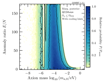
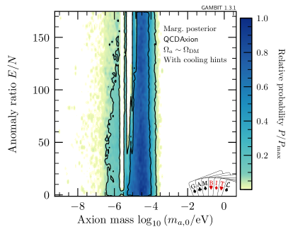
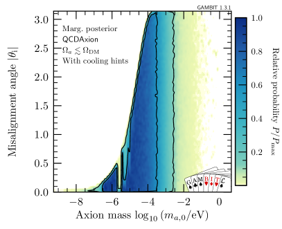
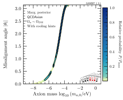
Selected results from the Bayesian analysis of QCD axions in combination with cooling hints can be found in Fig. 22. Compared to the Bayesian results without cooling hints in Fig. 16, we can see that the preferred mass regions in the $m_{a,0}$-$\theta_{\text{i}}$ plane get narrowed down slightly when we impose the DM relic density constraints as an upper limit (bottom left plot). However, for the anomaly ratio, $E/N$, this is not the case (top left plot). Generally speaking, these results identify the most credible regions for a compromise between QCD axions fitting the cooling hints and “naturally” not overproducing DM (which prefers masses of $\pazocal{O}(\text{$1100\text{\,}\mathrm{\SIUnitSymbolMicro eV}$})$, cf. Fig. 16). Despite the slight differences, which might also depend on the adopted priors, the overall results with and without cooling hints are remarkably similar. This is mainly due to the influence of the $R$ parameter likelihood included in both cases and its slight preference for non-zero couplings.

Figure 23: Marginalised posteriors (from T-Walk) for QCDAxion models with upper limits (left) and matching condition (right) for the observed DM relic density. We show the constraints on the axion-electron coupling, $C_{aee}$, without (grey lines) and with (black lines and coloured regions) the inclusion of cooling hints.

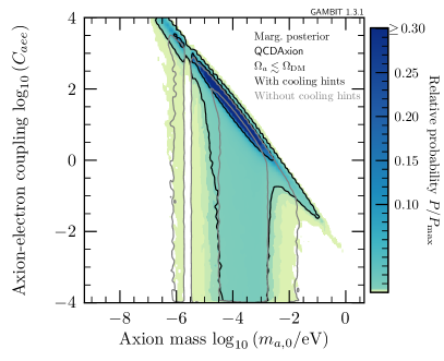
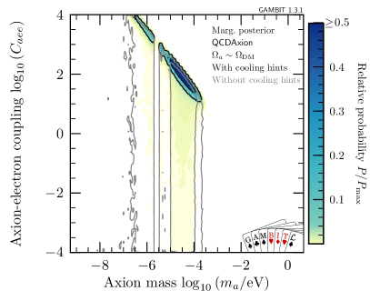
The influence of the cooling hints is illustrated further in Fig. 23, which shows the regions of highest posterior probability in the $m_{a,0}$-$C_{aee}$ parameter plane with and without the inclusion of cooling hints. Since the cooling hints strongly require $g_{aee}\sim$3\text{\times}{10}^{-13}$$ (cf. right panel of Fig. 11), we find the highest posterior probabilities along a line of constant $C_{aee}\,m_{a,0}$. The chosen range of $C_{aee}$ then implies that the cooling hints can only be explained for $m_{a,0}\mathrel{\hbox to0.0pt{\lower 4.0pt\hbox{$\sim$}\hss}\raise 1.0pt\hbox{$>$}}$0.3\text{\,}\mathrm{\SIUnitSymbolMicro eV}$$. For values of $C_{aee}\sim 1$, the cooling hints would point towards $\mathrm{meV}$-scale axions, which is incompatible with the requirement $\Omega_{a}\sim\Omega_{\text{DM}}$. This regime is therefore disfavoured in the right panel of Fig. 23. Not including the cooling hints essentially only results in a upper limit in the most credible mass regions close to where the line of constant $g_{aee}$ was (grey contours in Fig. 23), due to the $R$ parameter likelihood.

Figure 24: Marginalised posteriors (from T-Walk) for QCDAxion models with upper limits (density plots and black contour lines) and matching condition (grey contour lines) for the observed DM relic density. We show the constraints on the energy density in axions today, $\Omega_{a}h^{2}$, without (left) and with (right) the inclusion of cooling hints.

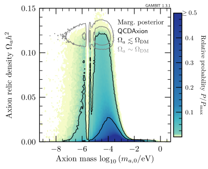
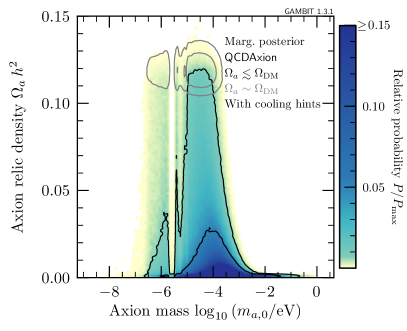
As mentioned before, QCD axions can account for both the cooling hints and all of the DM in the Universe (cf. Figs 21 and 22). However, because the posterior probability in Fig. 22 is normalised, one cannot infer from this plot if these solutions occur naturally or if considerable fine-tuning is required. Figure 24 gives an idea of the “naturalness” of QCDAxion DM by showing the marginalised posterior as a function of $m_{a,0}$ and $\Omega_{a}h^{2}$ (with and without the WD cooling hints). In the colour density plots of both panels in Fig. 24, we can see that the scan finds credible parts of the parameter space where axions account for a sizeable fraction of the DM while being consistent with all experiments and observations. The differences between including and not including the cooling hints regarding the preferred regions of $\Omega_{a}h^{2}$ are rather small, consistent with the other plots.

Similar to the discussion at the end of Sec. 5.3, we can infer the most credible regions for the relic abundance of axions as well as for $m_{a,0}$. The preferred axion mass is very similar with or without the inclusion of the cooling hints. Imposing the DM relic density as an upper limit, we find $$0.73\text{\,}\mathrm{\SIUnitSymbolMicro eV}$\leq m_{a,0}\leq$6.1\text{\,}\mathrm{meV}$$ at 95% credibility (equal-tailed interval); demanding that axions be all of the DM, this becomes $$0.53\text{\,}\mathrm{\SIUnitSymbolMicro eV}$\leq m_{a,0}\leq$0.13\text{\,}\mathrm{meV}$$. Including the cooling hints slightly modifies the preferred range for $\Omega_{a}h^{2}$. At 95% credibility (equal tails), $$5.2\text{\times}{10}^{-6}$\leq\Omega_{a}h^{2}\leq$0.11$$, corresponding to 0.004–94% of DM. The median value is $\Omega_{a}h^{2}=$7.1\text{\times}{10}^{-3}$$, or about 6% of the observed DM.

Figure 25: Marginalised posteriors (from T-Walk) for QCDAxion models with upper limits for the observed DM relic density (left) and matching condition (right). We show the constraints on the absolute value of the axion-photon coupling, $|g_{a\gamma\gamma}|$, together with models outside of the band of axion models (red line and shading) and the (frequentist) $2\sigma$ C.L. (dashed lines) for comparison. The prior-dependence of these results is investigated in Appendix D.

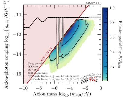
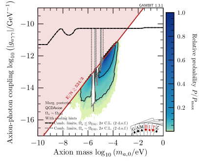
Finally, let us return to the $m_{a,0}$–$g_{a\gamma\gamma}$ parameter plane, as discussed in the GeneralALP model without cooling hints (see Fig. 12). In Fig. 25, we contrast the naïve bounds on the parameter space (from the phenomenological constraints on GeneralALP models and the maximum possible value of $E/N$) with the regions preferred by a Bayesian analysis. These regions are not only determined by the constraints from data (satisfying the cooling hints in both panels and matching the DM density in the right panel), but also by the fine-tuning in some parts of the parameter space. Fine tuning is necessary for avoiding overproduction of DM at small $m_{a,0}$, and for achieving low values of $g_{a\gamma\gamma}$ through cancellations between $E/N$ and $\widetilde{C}_{a\gamma\gamma}$ at large $m_{a,0}$ (cf. Eq. 22). For our adopted priors, the most credible parameter regions correspond to a few orders of magnitude around $m_{a,0}\sim$100\text{\,}\mathrm{\SIUnitSymbolMicro eV}$$ and $g_{a\gamma\gamma}\sim${10}^{-12}\text{\,}\mathrm{G}\mathrm{eV}^{-1}$$. In Appendix D we discuss how choosing different priors may affect these conclusions.

5.5.2 DFSZ- and KSVZ-type axions

DFSZ-type models have intrinsically larger coupling to electrons than KSVZ-type models, which only obtain their interactions with electrons at loop level. DFSZ models are therefore the natural choice to account for the potential WD cooling anomalies 1708.02111 , by way of an axion-electron coupling of $g_{aee}\sim$3\text{\times}{10}^{-13}$$.

Frequentist results.

Figure 26: Profile likelihoods (from Diver) for DFSZAxion-I (left) and DFSZAxion-II (right) models, compared to the profile likelihood for the QCDAxion model (grey lines), taking the observed DM abundance as an upper limit on the number of axions. Contours show the $1\sigma$ and $2\sigma$ confidence regions.

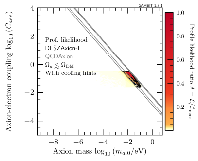
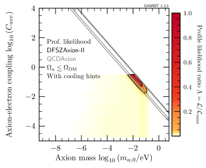
Fig. 26 shows the profile likelihood for the DFSZAxion-I and DFSZAxion-II models, compared to the band that maximises the profile likelihood for the QCDAxion model. Clearly both DFSZ-type models can accommodate the cooling hints with large axion-electron couplings. We already saw in Fig. 20 that even without the cooling hint likelihood, the KSVZAxion fails to achieve large $C_{aee}$ values; with cooling hints included, the highest likelihood regions for KSVZAxion models are therefore essentially the same as in Fig. 20.

Table 8: Best-fit values for DFSZAxion-I, DFSZAxion-II, and KSVZAxion models when imposing an upper limit on the DM relic density, $\Omega_{a}\mathrel{\hbox to0.0pt{\lower 4.0pt\hbox{$\sim$}\hss}\raise 1.0pt\hbox{$<$}}\Omega_{\text{DM}}$. In the final column, we compare the likelihood of the respective best-fit points to QCDAxion models. Note that the QCDAxion model has two more degrees of freedom than the KSVZ models, and one more than the DFSZ-type models.

Model	$E/N$	$\hat{m}_{a}$	$\hat{C}_{a\gamma\gamma}$	$\hat{g}_{a\gamma\gamma}$	$\hat{C}_{aee}$	$\hat{g}_{aee}$	$-2\Delta\ln(\hat{\mathcal{L}})$
		$\mathrm{meV}$		${10}^{-12}\text{\,}\mathrm{G}\mathrm{eV}^{-1}$	${10}^{-3}$	${10}^{-15}$
DFSZAxion-I	8/3	8.90	0.746	1.35	333	266	0.28
DFSZAxion-II	2/3	9.62	1.25	2.46	307	265	0.52
KSVZAxion	0	39.5	1.92	15.5	0.118	0.417	9.57
	2/3	59.4	1.25	15.2	0.0223	0.119	9.57
	5/3	316	0.252	16.2	0.210	5.94	9.49
	8/3	105	0.747	15.9	0.430	4.03	9.52

Table 8 gives the best-fit values for the six classic axion models that we consider in this section, under the requirement that they do not exceed the observed abundance of DM. We do not report best-fit values for $|\theta_{\text{i}}|$, as even with the maximum value included in our scans, axions only account for a few percent of the observed DM abundance. For each model, we calculate $\Delta\ln(\hat{\mathcal{L}})$, the logarithm of the ratio of the best-fit likelihood relative to the QCDAxion model. As anticipated, DFSZ-type models perform much better than KSVZAxions (at the expense of having one additional degree of freedom). This is because DFSZ-type models can easily reach the required axion-electron coupling to fit the cooling hints with masses of order $m_{a,0}\sim$10\text{\,}\mathrm{meV}$$ (as noted previously 1708.02111 ). For KSVZ-type axions, the masses required to naturally fit the cooling hints are about three to four orders of magnitude larger (see e.g. 24), and the associated axion-photon coupling is therefore in conflict with the $R$ parameter likelihood (as well as hot DM bounds, which are not included). Nevertheless, even for KSVZAxion models there is still a slight preference compared to having no axion at all, which corresponds to $-2\Delta\ln(\hat{\mathcal{L}})=10.54$.

For DFSZ-type models, the DFSZAxion-I model gives a better fit than the DFSZAxion-II model. This is due to the influence of the $R$ parameter likelihood, which combines with the cooling hints to force the axion-photon coupling to $g_{a\gamma\gamma}\mathrel{\hbox to0.0pt{\lower 4.0pt\hbox{$\sim$}\hss}\raise 1.0pt\hbox{$<$}}$2\text{\times}{10}^{-11}\text{\,}\mathrm{G}\mathrm{eV}^{-1}$$ (at 95% C.L.). The best-fit point is therefore a balance between reaching high enough $g_{aee}$ and minimising $g_{a\gamma\gamma}$. The maximum value of $C_{aee}$ for DFSZAxion-I models is about a factor of 1.08 larger than for DFSZAxion-II models, due to perturbativity constraints on $\tan(\beta^{\prime})$, whereas the axion-photon couplings are about a factor of 0.6 lower, yielding a better fit to the $R$ parameter likelihood at any given mass.

Next, let us briefly consider the case where we demand that the classic axion models provide all of the DM. This results in much poorer maximum likelihood values of around $-2\Delta\ln(\hat{\mathcal{L}})\approx 10.5$ compared to QCDAxion models for all KSVZ- and DFSZ-type models that we consider in this paper. This is not surprising because, unlike some other QCDAxion models, they cannot account for both the cooling anomalies and DM. The maximum-likelihood regions are also highly degenerate in this case, as none of the fits is actually “good” (with a maximum likelihood comparable to the case without any axion).

Finally, thanks to the model hierarchy shown in Fig. 1, we can perform nested hypothesis tests to determine whether or not the more constrained, specific DFSZAxion and KSVZAxion models are disfavoured compared to the broader class of QCDAxion models. Without the cooling hints, QCDAxion, DFSZAxion and KSVZAxion models cannot be discriminated. This situation changes if the WD cooling hints are taken into account. Imposing the measured DM density as an upper limit only, KSVZAxion models (null hypothesis) can be rejected with respect to QCDAxion models (alternative hypothesis) with a $p$-value of $0.008$. DFSZAxion models as a null hypothesis, on the other hand, cannot be rejected ($p\geq$0.47$$). If we instead demand that axions be all of DM, both DFSZAxion and KSVZAxion models can be rejected with respect to the QCDAxion model with $p$-values of $1.2\text{\times}{10}^{-3}$ and $5.3\text{\times}{10}^{-3}$, respectively.

Bayesian results.

Figure 27: Marginalised posteriors (from T-Walk) for DFSZAxion-I (left) and DFSZAxion-II (right) models, compared to the marginalised posterior for the QCDAxion model (grey lines), taking the observed DM relic density as an upper limit on the axion relic density and including cooling hints. We show only the 68.27% and 95.45% C.R.s for all models.

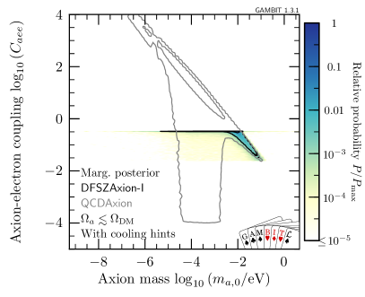
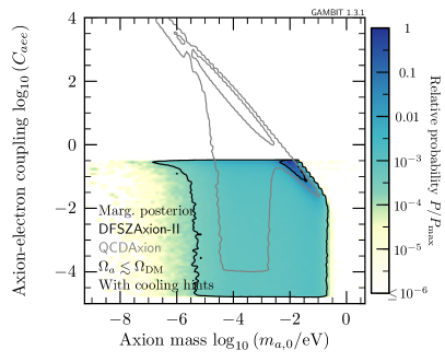
Figure 27 shows posteriors for the DFSZ-type models compared to the QCDAxion, in the $m_{a,0}$-$C_{aee}$ parameter plane (see also Fig. 23). These regions resemble the ones found in Fig. 26. The log prior on $\tan\beta^{\prime}$ enables both models to achieve sufficiently large values of $C_{aee}$ quite naturally, despite their structural differences. At first sight, DFSZAxion-II models appear to be able to occupy a larger region of parameter space in the 68.27% C.R. However, this is mainly a reflection of the effective prior on $C_{aee}$, which for the DFSZAxion-I model is strongly peaked towards the upper boundary of the accessible parameter space in Fig. 27. In contrast, the effective prior in $C_{aee}$ is almost flat in the DFSZAxion-II model. In terms of the fundamental parameters (i.e. $\tan\beta^{\prime}$), the credible parameter region in the DFSZAxion-I model is in fact larger, because the large values of $C_{aee}$ needed to explain the cooling hints can be achieved more easily.

Table 9: Odds ratios in favour of DFSZ- and KSVZ-type models, compared to the parent QCDAxion, as calculated from the nested sampling evidence estimates in MultiNest, and including the WD cooling hints. We either impose the DM relic density as an upper limit ($\Omega_{a}\mathrel{\hbox to0.0pt{\lower 4.0pt\hbox{$\sim$}\hss}\raise 1.0pt\hbox{$<$}}\Omega_{\text{DM}}$) or demand that axions be all of DM ($\Omega_{a}\sim\Omega_{\text{DM}}$). Note that the estimated uncertainties on the evidence values are small enough that the corresponding uncertainties on the odds ratios are negligible.

Model	DFSZAxion-I	DFSZAxion-II	KSVZAxion
$E/N$	$8/3$	$2/3$	$0$	$2/3$	$5/3$	$8/3$
Odds ($\Omega_{a}\mathrel{\hbox to0.0pt{\lower 4.0pt\hbox{$\sim$}\hss}\raise 1.0pt\hbox{$<$}}\Omega_{\text{DM}}$)	3:1	1:1	1:3	1:2	1:2	1:2
Odds ($\Omega_{a}\sim\Omega_{\text{DM}}$)	1:5	1:5	1:6	1:6	1:6	1:6

To investigate the consequences of fine-tuning in more detail, we consider all models in a Bayesian model comparison. The resulting odds ratios can be found in Table 9. If we impose the DM relic density as an upper limit, the odds ratios are still mostly inconclusive. However, for the DFSZAxion-II and KSVZAxion models, the trend swings in favour of the broader class of QCDAxion models when cooling hints are added to the analysis. In contrast, the DFSZAxion-I model fares better than the QCDAxion, with an odds ratio of 3:1. If we combine this 3:1 odds ratio with the 2:1 preference for the QCDAxion model over most KSVZAxion models, there is at least a 6:1 positive preference for the DFSZAxion-I model over all KSVZAxion models. This preference is not surprising, given the differences in the natural axion-electron coupling strength in these models.

If we demand that axions solve the cooling hints and constitute all of DM, model comparison confirms quantitatively (with ratios of $\leq\text{1:5}$) that there is a positive preference for the QCDAxion over the DFSZ- and KSVZ-type models. This is because we allowed for much larger values of $C_{aee}$ with QCDAxion models than with DFSZ- and KSVZ-type models. In fact, the one-dimensional marginal posterior for the QCDAxion electron coupling peaks at $C_{aee}\sim 100$ ($C_{aee}\sim 50$ if we impose the DM relic density as an upper limit), whereas the DFSZ and KSVZ models are limited to couplings of less than one. However, it should be noted that QCDAxion models with such a large coupling are not expected from traditional axion models, and may therefore pose a challenge for model building.

6 Conclusions

In this study we presented the first global fits of axion models in the pre-inflationary PQ symmetry-breaking scenario, using frequentist and Bayesian methods. We identified the most viable regions of parameter space for these models and discussed the effect of adding cooling hints seen in white dwarfs. We not only considered the phenomenological parameter space, but also the underlying parameters in a generic QCD axion model and six specific DFSZ- and KSVZ-type models. We extended previous results in the literature by including various nuisance parameters and by quantitatively considering the fine-tuning of the initial misalignment angle.

We found, in agreement with previous work, that QCD axion models are viable as explanations for both the observed cold dark matter and the white dwarf cooling hints. We showed that, for a broader class of QCDAxion models than what is traditionally considered, these can be achieved simultaneously. We also quantitatively confirmed that this is not possible for six specific DFSZ- and KSVZ-type models. However, if the condition of being all the dark matter in the Universe is relaxed, we found that DFSZAxion-I models are positively preferred over DFSZAxion-II models, and over all four KSVZAxion models that we investigated.

We determined the most credible predicted ranges for the QCD axion mass and its cosmological abundance in the Bayesian statistical framework. Although these results are somewhat prior-dependent, QCDAxions appear likely to be a cosmologically relevant (but probably not dominant) component of dark matter. Moreover, the most credible axion mass range is within reach of current and planned haloscope experiments.

Global fits of QCD axions and axion-like particles have the potential to confirm and refine previously known phenomenological statements about the relevant parameter spaces (e.g. exclusion limits, existence of fine-tuning, compatibility with cooling hints and dark matter). In other cases, they offer new and more rigorous insights (e.g. model comparison, most credible parameter regions). This is true in particular for the Bayesian analyses that we performed in this paper, because they inherently take fine-tuning into account. Due to the orthogonality of constraints and the insufficient sensitivity of most experiments, it is not (yet) possible to decisively probe the axion parameter space in the pre-inflationary PQ symmetry-breaking scenario, but it is realistically possible to target the most likely versions of QCD axion and axion-like particle models in the near future (see Ref. 1801.08127 for a recent review of upcoming axion searches).

The axion routines that we developed for this paper are publicly available in DarkBit within GAMBIT 1.3.1. Statistical samples and input files from this study are freely available from Zenodo Zenodo_axions .

Appendix A Integrating solar models for the signal prediction in CAST

To obtain the axion flux at Earth from axion-photon interactions, we need four inputs from a solar model: the solar radius $R_{\odot}$, the temperature $T(r)$, the plasma frequency $\omega_{\text{pl}}(r)$ and the screening scale $\kappa_{\text{s}}(r)$ (see Eqs. 33–36). While $T(r)$ can be obtained directly from solar model files, $\omega_{\text{pl}}(r)$ and $\kappa_{\text{s}}(r)$ have to be calculated using the mass density $\rho(r)$ and the mass fractions $X_{i}(r)$ for each ion/atom with label $i$ using (34). Assuming that the plasma is fully ionised, we can recast the equations into the following form book_raffelt_laboratories :

$$\kappa_{\text{s}}^{2}(r) =\frac{4\pi\alpha_{\text{EM}}}{T(r)}\frac{\rho(r)}{m_{\text{u}}}\sum_{i}\frac{X_{i}(r)Z_{i}}{A_{i}}\left(1+Z_{i}\right)\,,$$ (58)

$$\text{and}\quad\omega_{\text{pl}}^{2}(r) =\frac{4\pi\alpha_{\text{EM}}}{m_{e}}\frac{\rho(r)}{m_{\text{u}}}\sum_{i}\frac{X_{i}(r)Z_{i}}{A_{i}}\,,$$ (59)

where $m_{\text{u}}$ is the atomic mass unit, $r$ is the distance from the centre of the Sun in units of $R_{\odot}$, and $Z_{i}$ and $A_{i}$ are the charge and atomic weight of the $i$th element. Note that the approximation of full ionisation is justified almost everywhere inside the Sun, i.e. $r\lesssim 0.95$. As the largest contribution to the axion flux comes from the innermost region ($r\mathrel{\hbox to0.0pt{\lower 4.0pt\hbox{$\sim$}\hss}\raise 1.0pt\hbox{$<$}}0.2$ hep-ex/0702006 ), we can safely employ this assumption. For elements tracked by the solar model in bulk (i.e. without isotopic information), we calculate the mean atomic weights $A_{i}$ using the isotopic composition of Ref. AGSS , with values based on the terrestial composition updated to use more recent data 10.1515/pac-2015-0305 .

The expected number of photons in the energy range $[E_{j},E_{j+1}]$ is

$$s_{j}=\int_{E_{j}}^{E_{j+1}}\!\mathcal{E}(E)\;\frac{\mathrm{d}\Phi(E)}{\mathrm{d}E}\;\mathrm{d}E\,,$$ (60)

where $\mathcal{E}$ is the effective exposure and $\mathrm{d}\Phi/\mathrm{d}E$ is the combined photon spectrum from axion-electron and axion-photon contributions. We neglect the energy dispersion of the CAST detector, as it is always less than about 0.2 keV hep-ex/0702006 , and therefore smaller than or comparable to the bin width of the CAST analyses (0.3 keV and 0.5 keV respectively for the 2007 and 2017 analyses). We provide tabulated data within DarkBit for the effective exposure $\mathcal{E}$; this can be found in DarkBit/data as dataset_EffectiveExposure.dat, where dataset is either CAST2007 or CAST2017_X, where X corresponds to the data sets A to L in Ref. 1705.02290 . All other files that we mention in the following can be found in the same folder.

Note that performing the energy integration in (60) after the density integral in (36) is only possible because all contributions to the integral are for energies greater than $\omega_{\text{pl}}(0)\approx$0.3\text{\,}\mathrm{keV}$$. For energies lower than $\omega_{\text{pl}}$, axions cannot be produced from the plasma and the square root in (36) becomes ill-defined.

To obtain the contribution to $\mathrm{d}\Phi/\mathrm{d}E$ from axion-photon interactions, we integrate (35) and (36) over $r$ and $\rho$, using the adaptive 51 point Gauss-Kronrod rule gsl_integration_qag, from the gsl library. We obtain quantities necessary for these integrations (temperature, etc.) by interpolating the solar model linearly in radius. For the contribution to $\mathrm{d}\Phi/\mathrm{d}E$ from axion-electron interactions, we use the spectrum published in Ref. 1310.0823 and redistribute it as Axion_Spectrum_AGSS09met_old_gaee.dat.

The peaks in the spectrum from axion-electron interactions specifically require using an algorithm that takes them into account as singularities. We therefore compute the contribution from axion-electron interactions to the signals $s_{j}$ (60) using the gsl_integration_qagp integrator of the gsl library. For the axion-photon contribution to the signal, we again use the 51-point Gauss-Konrod rule. We perform all signal calculations to a relative accuracy of $10^{-6}$.

We compute signals at reference values of $g_{a\gamma\gamma}=${10}^{-10}\text{\,}\mathrm{G}\mathrm{eV}^{-1}$$ and $g_{aee}=${10}^{-13}$$, at 183 mass values ranging from ${10}^{-3}{10}^{2}\text{\,}\mathrm{eV}$. We use unequally spaced mass values, as the density of points needs to be higher in certain regions to obtain good interpolating functions. We provide these pre-calculated signal count files as dataset_ReferenceCounts_solarmodel_coupling.dat, where dataset refers to CAST2007 or CAST2017_X results, solarmodel is the name of the solar model, and coupling is either the contribution from axion-photon interactions (gagg) or axion-electron interactions (gaee).

For the axion-photon contribution ($\textit{\color[rgb]{0,0.66796875,0}\definecolor[named]{pgfstrokecolor}{rgb}{0,0.66796875,0}\footnotesize{coupling}}=\texttt{gagg}$), we provide these files for the GS98 10.1023/A:1005161325181 ; 1611.09867 , AGSS09ph 0909.2668 , AGSS09met_old 0909.2668 and AGSS09met 1611.09867 models. For the axion-electron contribution ($\textit{\color[rgb]{0,0.66796875,0}\definecolor[named]{pgfstrokecolor}{rgb}{0,0.66796875,0}\footnotesize{coupling}}=\texttt{gaee}$), where a direct calculation of $\mathrm{d}\Phi/\mathrm{d}E$ is not easily performed, we provide a single file based on the earlier iteration of the AGSS09met model (AGSS09met_old); this corresponds to the model used in Ref. 1310.0823 to compute the spectrum that we ship in DarkBit.

The user may choose which solar model to employ from the Rules section of the YAML file, using the keys solar_model_gagg and solar_model_gaee, with dataset being CAST2007 or CAST2017 (no suffix in this case, as the CAST 2017 likelihood combines all the results):

⬇

Rules:

- capability: @\metavar{dataset}@_signal_vac

options:

solar_model_gagg: @\metavar{solarmodel}@

solar_model_gaee: @\metavar{solarmodel}@

If these options are left unspecified, the defaults will be chosen. For the axion-photon coupling, this is AGSS09met 1611.09867 ; for the axion-electron coupling, the default is AGSS09met_old 0909.2668 . If the corresponding dataset_ReferenceCounts_solarmodel_coupling.dat file cannot be found, DarkBit will attempt to create such a file by solving (60). For the axion-photon coupling, it will attempt to do this on the basis of a provided solar model file, which should be called SolarModel_solarmodel.dat. We have included the solar model file SolarModel_AGSS09met.dat from Ref. 1611.09867 as an example of the expected formatting. For the axion-electron coupling, DarkBit will attempt to generate the relevant dataset_ReferenceCounts_solarmodel_gaee.dat file on the basis of a provided spectrum file Axion_Spectrum_solarmodel_gaee.dat. If the relevant solar model or spectrum file cannot be located, or has the wrong format, GAMBIT will terminate. Note that this will currently happen for any choice of solar_model_gaee except for the default value. However, if the user can provide the spectrum file for any other model, the calculation will go ahead.

Appendix B Numerical implementation of the solution to the axion field equation

The most general equation of motion for a scalar field $\phi(t,\mathbf{x})$ in the background of a Friedmann-Robertson-Walker-Lemaître universe with Hubble parameter $H\equiv\dot{a}/a$ and potential $V$ is given by (weinberg_cosmology, , app. B.12)

$$\ddot{\phi}+3H(t)\dot{\phi}+\frac{\Delta\phi}{a^{2}(t)}+V^{\prime}[\phi]=0\,,$$ (61)

while the energy density associated with $\phi$ can be calculated using:

$$\varepsilon=\frac{1}{2}\dot{\phi}^{2}-\frac{1}{2a^{2}(t)}\left(\nabla\phi\right)^{2}+V[\phi]\,.$$ (62)

To obtain the energy density in axions today, it is sufficient to solve the homogeneous field equation for $\theta\equiv a/f_{a}$, the normalised axion field:

$$\ddot{\theta}+3H\dot{\theta}+\frac{V^{\prime}[\theta]}{f_{a}^{2}}=0\,.$$ (63)

We assume the potential

$$V\left[\theta\right]=f_{a}^{2}\,m_{a}^{2}\left[1-\cos\left(\theta\right)\right]\,,$$ (64)

for QCD axions and ALPs alike. For QCD axions, this is a reasonable approximation to the full potential DiVecchia:1980yfw . The axion energy density $\varepsilon_{a}\simeq\rho_{a}$ from (62) is therefore given by

$$\rho_{a}=\frac{1}{2}f_{a}^{2}\,\dot{\theta}^{2}+f_{a}^{2}\,m_{a}^{2}\left[1-\cos\left(\theta\right)\right]\,.$$ (65)

The initial conditions for (63) are some initial misalignment angle $\theta(0)\equiv\theta_{\text{i}}$ and vanishing initial derivatives $\dot{\theta}(0)\equiv 0$. For early times, the solution of (63) is a constant value, $\theta(t)=\theta_{\text{i}}$. The behaviour only changes around the oscillation time $T_{\text{osc}}$, defined as the point when $3H(T_{\text{osc}})=m_{a}(T_{\text{osc}})$.

Assuming that the scale factor $a$ is a monotonically increasing function of cosmic time $t$, and that the temperature $T$ is a monotically decreasing function of $t$, we may re-write (63) as

$$\mathrm{D}_{X}\theta+\frac{V^{\prime}\left[\theta\right]}{f_{a}^{2}}=0\,,$$ (66)

where $X=t,\,\alpha,\,\tau$ with $\alpha\equiv a/a_{\text{osc}}$, $\tau\equiv T/T_{\text{osc}}$ and

$$\mathrm{D}_{t} =\frac{\mathrm{d}^{2}}{\mathrm{d}t^{2}}+3H\frac{\mathrm{d}}{\mathrm{d}t}\,,$$ (67)

$$\mathrm{D}_{\alpha} =H^{2}\alpha^{2}\left[\frac{\mathrm{d}^{2}}{\mathrm{d}\alpha^{2}}+\left(\frac{1}{\alpha}+\frac{1}{H}\frac{\mathrm{d}H}{\mathrm{d}\alpha}\right)\frac{\mathrm{d}}{\mathrm{d}\alpha}\right]\,,$$ (68)

$$\mathrm{D}_{\tau} =\left(\frac{H\alpha}{\alpha^{\times}}\right)^{2}\left[\frac{\mathrm{d}^{2}}{\mathrm{d}\tau^{2}}+\left(\frac{H^{\times}}{H}+\frac{\alpha^{\times}}{\alpha}-\frac{\alpha^{\times\times}}{\alpha^{\times}}\right)\frac{\mathrm{d}}{\mathrm{d}\tau}\right]\,,$$ (69)

where ^× denotes derivatives w.r.t. $\tau$. Conservation of entropy can subsequently be used to relate $\alpha$ and temperature:

$$\alpha=\left(\frac{g_{S}(T)}{g_{S}({T}_{\text{osc}})}\right)^{-1/3}\tau^{-1}\equiv\gamma(\tau)/\tau\,.$$ (70)

Equation (69) has the advantage that an explicitly temperature-dependent axion mass or the effective relativistic degrees of freedom, $g$ and $g_{S}$, can be easily incorporated. The various terms can be further simplified as follows:

$$\frac{\alpha^{\times}}{\alpha} =\frac{\gamma^{\times}}{\gamma}-\frac{1}{\tau}\,,$$ (71)

$$\frac{\alpha^{\times\times}}{\alpha^{\times}} =\frac{\alpha^{\times\times}}{\alpha}\,\frac{\alpha}{\alpha^{\times}}=\frac{\tau\gamma^{\times\times}}{\tau\gamma^{\times}-\gamma}-\frac{2}{\tau}\,.$$ (72)

Rescaling $\vartheta\equiv\theta/\theta_{\text{i}}$, we may use (69) to rewrite (66) as

$$\vartheta^{\times\times}+\frac{F_{2}(\tau)}{\tau}\,\vartheta^{\times}+\left(\frac{F_{1}(\tau)m_{a}(\tau)}{\tau H(\tau)}\right)^{2}\,\frac{\sin\left(\theta_{\text{i}}\vartheta\right)}{\theta_{\text{i}}}=0\,,$$ (73)

where the auxiliary functions $F_{i}$ for $i=1,2$ are given by

$$F_{1}(\tau) =-1+\frac{\tau\gamma^{\times}}{\gamma}=-\left(1+\frac{\tau}{3}\frac{g_{S}^{\times}}{g_{S}}\right)\,,$$ (74)

$$F_{2}(\tau) =\phantom{-}2+\frac{\tau H^{\times}}{H}-\frac{\tau^{2}g_{S}^{\times\times}+4\tau g_{S}^{\times}}{\tau g_{S}^{\times}+3g_{S}}\,,$$ (75)

$$=\phantom{-0+}\frac{\tau}{2}\frac{g^{\times}}{g}-\frac{\tau^{2}g_{S}^{\times\times}+4\tau g_{S}^{\times}}{\tau g_{S}^{\times}+3g_{S}}\,,$$ (76)

where we assume a radiation-dominated universe, $H\propto\sqrt{g(T)}\,T^{2}$, for the last line. We use interpolated values for (74) and (76) based on the analytic forms for the effective degrees of freedom in Ref. 0910.1066 . The tables used for this procedure are included in GAMBIT.

Note that if the changes in the effective degrees of freedom are not important, $F_{1}(\tau)\approx-1$, $F_{2}(\tau)\approx 0$, and the field equation (73) reads in the harmonic limit of $\left|\theta_{\text{i}}\right|\ll 1$:

$$\theta^{\times\times}\approx-\left(\frac{m_{a}(\tau)}{H\tau}\right)^{2}\,\theta\,,$$ (77)

i.e. we obtain the approximate behaviour of a (damped) harmonic oscillator. In that limit, the comoving axion number density $n_{a}\equiv\rho_{a}a^{3}/m_{a}$ is conserved on average. We can therefore stop integrating the differential equation once specified conditions for $m_{a}/3H$ and $\theta$ are met. Because the solution $\theta(t)$ oscillates as a function of time or temperature, we define a peak amplitude $\hat{\theta}$ in order to check that $\left|\theta(t_{\star})\right|\ll 1$ from some time $t_{\star}$:

$$\hat{\theta}(t)\equiv\frac{\sqrt{2\rho_{a}(t)}}{f_{a}m_{a}(t)}\,.$$ (78)

In the harmonic limits, (78) indeed coincides with the amplitude of oscillation when all the energy of the field is stored in the potential part of the energy density. Once the axion field starts to oscillate, fulfilment of the condition $\hat{\theta}\ll 1$ indicates that the harmonic limit has been achieved. This provides much clearer limiting behaviour than e.g. $|\theta|$.

We use the gsl implementation of Brent’s method to solve for $T_{\text{osc}}$ to a precision of ${10}^{-6}$. We then impose the initial conditions at some relatively high temperature $\tau_{\text{start}}=${10}^{5}$$, and evolve the differential equation with gsl_odeiv2_step_bsimp until some relative temperature $\tau_{\text{stop}}$ for which $m_{a}/3H>${10}^{3}$$ and $\hat{\theta}<${10}^{-2}$$. We then calculate the energy density from realignment axions today using the conservation of comoving number density

$$\rho_{a}=\frac{m_{a,0}}{m_{a,\star}}\,\frac{g_{S}(T_{\text{CMB}})}{g_{S}(T_{\star})}\,\left(\frac{T_{\text{CMB}}}{T_{\star}}\right)^{3}\,\rho_{a,\star}\,,$$ (79)

where $T_{\text{CMB}}$ is the CMB temperature.

Appendix C H.E.S.S. likelihood implementation details

Figure 28: Detailed description of our implementation of the H.E.S.S. exclusion limits from gamma-ray spectral distortions of PKS 2155-304 (Fig. 8). We show the points that form the basis of our interpolation: points directly from the exclusion curves (all blue triangles, circles and stars), estimated points (squares) as well as points directly inferred from the interpolation scheme (diamonds). See the main text for further details.

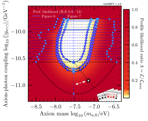
Our approximation of the H.E.S.S. likelihood is based on the information provided in Figs 6 and 7 of Ref. 1311.3148 on limits on axion-photon conversion in galactic cluster magnetic fields. We choose 13 lines of constant axion-photon coupling (corresponding to specific values of the axion decay rate $\Gamma$ in their figure) that intersect with the exclusion curves at least five times (dashed black and blue horizontal lines and blue circles in Fig. 28).

We subsequently define a family of one-dimensional natural cubic splines along each dashed line by including two additional points outside of the known data. We optimise each of those splines by iteratively modifying the locations of the additional points along the dashed lines, until the values and first derivatives of the splines at the additional points go to zero (blue diamonds in Fig. 28). This forcibly prevents ringing, ensuring that the interpolated log-likelihood is negative everywhere. To evaluate the log-likelihood at a given axion mass on one of the horizontal dashed lines, we use the resultant interpolating cubic spline from the fitting procedure. If a coupling value of interest sits between two horizontal dashed lines, we interpolate linearly between the values at a given mass on the adjacent dashed lines. We assign zero log-likelihood to all points outside of the area defined by the exterior points (blue diamonds).

This leaves two more regions in Fig. 28. The first is at higher couplings, where Fig. 6 of Ref. 1311.3148 does not show any limits, but Fig. 7 does (dotted horizontal lines and blue triangles in Fig. 28). To complete the likelihood curve families in this region, we infer additional points (by eye; light blue squares in Fig. 28) and follow the procedure described in the previous paragraph. We assign zero log-likelihood to all couplings above the uppermost horizontal line in Fig. 28.

At low couplings, less than five contours are available for interpolating (inverted triangles in Fig. 28). Here, we construct a single cubic spline in the vertical direction (blue stars and vertical dot-dash line in Fig. 28), in order to determine an exterior point at low coupling (the diamond at the bottom of the plot). We define three parabolae, based on nine points: the set of two diamonds and four outer circles on the dashed black line around $g_{a\gamma\gamma}=$e-10.6\text{\,}\mathrm{G}\mathrm{eV}^{-1}$$, the two stars below this line, and the one diamond at the bottom of the plot. We designate the lower parabola, passing through the exterior point (bottommost diamond) at low coupling and drawn as a dashed black curve, as the zero-log-likelihood contour. We use the middle parabola to model the 99% C.L. exclusion curve, and the upper one to model the 95% C.L. curve. These three parabolae allow us to map any point (represented by the white star) inside the lower parabola to a likelihood, by interpolating between the three parabolae. We do this using the one-dimensional spline constructed along the central vertical axis, using as input to the interpolation the position of the point in question between the central star and the zero-log-likelihood parabola. We carry out all interpolations in log space for both the axion mass and the axion-photon coupling.

Appendix D Prior-dependence of results

For QCD axions some prior choices are relatively straightforward (such as the use of a flat prior for $\theta_{\text{i}}$) or do not have a significant impact on the results (such as the prior assignments for the well-constrained nuisance parameters). In general, however, the prior beliefs can have a significant impact on the posteriors and Bayes factors, especially in the absence of constraining data. In this appendix, we investigate different prior choices for the parameters $f_{a}$, $C_{aee}$, and $E/N$ in order to assess the robustness of our results and to understand how our conclusions may be affected by a variation of priors. All the new results that we present in this appendix are based on MultiNest runs only, as we need the evidence values for examining the impacts of priors on model comparison, but are not sufficiently interested in the finer details of posterior maps to warrant also running T-Walk.

Figure 29: Marginalised posteriors for QCDAxion models with three alternative priors. Here we impose the observed DM relic density as an upper limit. We show the one-dimensional posterior for the axion mass without the cooling hints (left; to be compared to the right panel of Fig. 17) and the two-dimensional posterior for $m_{a,0}$ vs $g_{a\gamma\gamma}$, including the cooling hints (right; to be compared with Fig. 25). The priors adopted in the main part of this study are marked in grey in the left panel, and in the colour scale and black contours in the right panel.

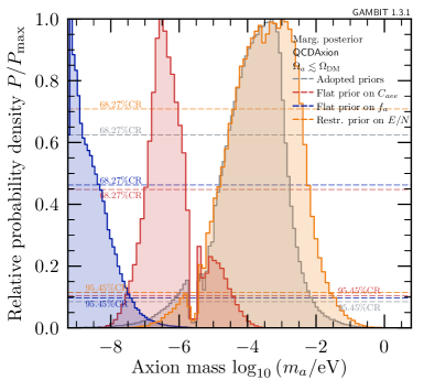
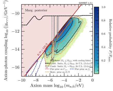
First, let us revisit the determination of the most credible regions for the axion mass in QCDAxion models from Sec. 5.3. The left panel of Fig. 29 shows the marginalised posterior distribution for the axion mass, $m_{a,0}$, for a number of alternative priors. The grey line and shading correspond to the prior choice made in the main text (right panel of Fig. 17). We can see that choosing a flat prior on either $C_{aee}$ or $f_{a}$ shifts the most credible region for the axion mass to lower masses. The effect is more extreme for a flat prior on $f_{a}$ than for a flat prior on $C_{aee}$. On the other hand, restricting the prior of the anomaly ratio to $E/N\leq 170/3$ (the highest values achievable in KSVZ-type models) does not have a significant impact on the result.

The different prior choices also alter the most credible regions of the axion-photon couplings (cf. Fig. 25). The resulting posterior distributions are shown in the right panel of Fig. 29. As expected, priors that imply a preference for smaller axion masses also lead to a preference for smaller values of $g_{a\gamma\gamma}$, while changes in prior that do not significantly affect the most probable region for $m_{a,0}$ also do not impact the findings for $g_{a\gamma\gamma}$ very much. In particular, for the alternative priors on $E/N$ and $C_{aee}$, the regions of highest posterior density still overlap with the region that we obtained with our adopted prior, whereas the regions resulting from a flat prior on $f_{a}$ are almost completely disjoint from the others.

The preference for very small axion masses for the case of a flat prior on $f_{a}$ is a direct consequence of the relation between $f_{a}$ and $m_{a,0}$, which implies that the prior probability for $m_{a,0}$ is strongly peaked at the lowest possible axion masses. This prior then overwhelms the preference for large $m_{a,0}$ from the combination of tuning in the initial misalignment angle and the relic density requirement. In other words, the preferred mass range in this case is dictated almost entirely by the assumed prior. A log prior on $f_{a}$, on the other hand, essentially corresponds to a log prior on $m_{a,0}$, which has the important advantage that any preference in the axion mass range is the result of phenomenological requirements on the model. A logarithmic prior for $f_{a}$ is therefore less informative than a flat one, which favours a particular scale of new physics near the upper end of the prior range.

However, it is also important to determine how changing the range of the logarithmic prior impacts our results. Taking the example of the grey curve in the left panel of Fig. 29 (canonical priors, no cooling hints, $\Omega_{a}\mathrel{\hbox to0.0pt{\lower 4.0pt\hbox{$\sim$}\hss}\raise 1.0pt\hbox{$<$}}\Omega_{\text{DM}}$), we find that restricting the log prior to $f_{a}\in[10^{7},\,10^{15}]\,$\mathrm{GeV}$$ results in a 95% equal-tailed credible interval for the axion mass of $$0.64\text{\,}\mathrm{\SIUnitSymbolMicro eV}$\leq m_{a,0}\leq$6.8\text{\,}\mathrm{meV}$$, compared to $$0.60\text{\,}\mathrm{\SIUnitSymbolMicro eV}$\leq m_{a,0}\leq$7.1\text{\,}\mathrm{meV}$$ for the prior range that we adopted in the main paper ($f_{a}\in[10^{6},\,10^{16}]\,$\mathrm{GeV}$$). Narrowing this range further to $f_{a}\in[10^{8},\,10^{14}]\,$\mathrm{GeV}$$ also compresses the interval slightly more: $$0.81\text{\,}\mathrm{\SIUnitSymbolMicro eV}$\leq m_{a,0}\leq$6.1\text{\,}\mathrm{meV}$$. Clearly the range of the logarithmic prior on $f_{a}$ has little impact on our results. The median values and credible intervals of $\Omega_{a}$ are even more stable, with the lower bound of the 95% equal-tailed credible interval slightly increasing from $3.7\text{\times}{10}^{-6}$ to $4.3\text{\times}{10}^{-6}$ for $f_{a}\in[10^{8},\,10^{14}]\,$\mathrm{GeV}$$ (corresponding to about 0.004% of the cosmological density of DM).

Table 10: Odds ratios in favour of DFSZ- and KSVZ-type models, compared to the parent QCDAxion model, as calculated from nested sampling evidence estimates by MultiNest. We impose the DM relic density as an upper limit ($\Omega_{a}\mathrel{\hbox to0.0pt{\lower 4.0pt\hbox{$\sim$}\hss}\raise 1.0pt\hbox{$<$}}\Omega_{\text{DM}}$). Note that the estimated uncertainties on the evidence values are small enough that the corresponding uncertainties on the odds ratios are negligible.

Model	DFSZAxion-I	DFSZAxion-II	KSVZAxion
$E/N$	$8/3$	$2/3$	$0$	$2/3$	$5/3$	$8/3$
Priors adopted in this study
Odds (w/o WD cooling)	2:1	2:1	2:1	2:1	2:1	2:1
Odds (with WD cooling)	3:1	1:1	1:3	1:2	1:2	1:2
Reduced prior range on $E/N$ in QCDAxion models
Odds (w/o WD cooling)	1:1	2:1	2:1	2:1	2:1	2:1
Odds (with WD cooling)	2:1	1:1	1:4	1:4	1:3	1:4
Flat prior on $C_{aee}$ in QCDAxion models
Odds (w/o WD cooling)	24:1	29:1	29:1	31:1	34:1	32:1
Odds (with WD cooling)	4:1	2:1	1:2	1:2	1:2	1:2
Flat prior on $f_{a}$ in all models
Odds (w/o WD cooling)	1:1	1:1	1:1	1:1	1:1	1:1
Odds (with WD cooling)	1:1	1:1	1:1	1:1	1:1	1:1

We also calculate the Bayes factors for KSVZ- and DFSZ-type models compared to QCDAxion models, adopting the alternative priors for the appropriate models. The resulting odds ratios are given in Table 10, in addition to the values for the priors that we adopt in Sec. 5.

As in Fig. 29, adopting a reduced range for the anomaly ratio $E/N$ has little impact, slightly increasing the odds in favour of KSVZ-type models. Choosing the alternative prior on the axion-electron coupling constant, $C_{aee}$, the odds in favour of KSVZ- and DFSZ-type models increase by an order of magnitude (if cooling hints are not included). This is because the flat prior on $C_{aee}$ causes a preference for large $f_{a}$ (smaller $m_{a,0}$). This, in turn, implies a considerable fine-tuning in $\theta_{\text{i}}$ in order to avoid overproducing DM. After including the cooling hints, axion-electron interactions are much more tightly constrained by data, and the prior-dependence of the odds ratios is reduced.

Finally, a flat prior on $f_{a}$ favours the lowest allowed axion masses in all models. This results in even more fine-tuning of the initial misalignment angle than using a flat prior on $C_{aee}$ for QCDAxion models. However, although the Bayesian evidence in QCDAxion models is drastically reduced, the odds ratios in favour of KSVZ- and DFSZ-type models turn out to be 1:1. This is because the alternative prior is applied to all models: the fine-tuning required to overcome the prior pushes all evidences equally low, washing out any preference one way or another from the data.

We see that prior choice can indeed significantly influence the results of our analysis. This is true in particular for a flat prior on $f_{a}$, where the prior-dependence dominates the results. On the other hand, we also saw that data with a strong preference for certain model parameter values, such as the cooling hints, can reduce the prior-dependence. In the face of more such data, the impact of prior choices tends to become less pronounced, ideally leaving only the physically-motivated prior on the initial misalignment angle able to influence final results.

Appendix E Overview of new capabilities

Table 11: New, axion-related capabilities for the DarkBit module in GAMBIT.

Capability	Function (Return Type): Brief Description	Dependencies
QCDAxion_ZeroTemperatureMass	QCDAxion_ZeroTemperatureMass_Nuisance_lnL (double): Nuisance likelihood for the QCD-related energy scale $\Lambda_{\chi}$, which defines the low-energy QCD axion mass.
QCDAxion_TemperatureDependence	QCDAxion_TemperatureDependence_Nuisance_lnL (double): Nuisance likelihood for the parameters $\beta$ and $T_{\chi}$, which define the temperature dependence of the QCD axion mass for high temperatures.
QCDAxion_AxionPhotonConstant	QCDAxion_AxionPhotonConstant_Nuisance_lnL (double): Nuisance likelihood for the contribution of axion-pion interactions in the chiral Lagrangian to the axion-photon coupling.
ALPS1_signal_vac	calc_ALPS1_signal_vac (double): Calculates the signal prediction for one data frame of the ALPS 1 experiment (evacuated setup).
ALPS1_signal_gas	calc_ALPS1_signal_gas (double): Calculates the signal prediction for one data frame of the ALPS 1 experiment (setup filled with Argon gas).
lnL_ALPS1	calc_lnL_ALPS1 (double): Log-likelihood for all runs of the ALPS 1 experiment.	ALPS1_signal_vac, ALPS1_signal_gas
CAST2007_signal_vac*	calc_CAST2007_signal_vac (std::vector<double>): Signal prediction for a 2004 vacuum run of the CAST experiment.
lnL_CAST2007	calc_lnL_CAST2007 (double): Log-likelihood for CAST 2007 experimental results.	CAST2007_signal_vac
CAST2017_signal_vac*	calc_CAST2017_signal_vac (std::vector<std::vector<double>>): Signal prediction for the combined 2013, 2014 and 2015 vacuum runs of the CAST experiment.
lnL_CAST2017	calc_lnL_CAST2017 (double): Log-likelihood for CAST 2017 experimental results.	CAST2017_signal_vac
Haloscope_signal	calc_Haloscope_signal (double): Calculates the relative expected signal for a haloscope ignoring experimental parameters and mass dependence.
lnL_Haloscope_ADMX1	calc_lnL_Haloscope_ADMX1 (double): Log-likelihood for the combined ADMX 1998 to 2011 experimental results.	Haloscope_signal
lnL_Haloscope_ADMX2	calc_lnL_Haloscope_ADMX2 (double): Log-likelihood for the ADMX 2018 experimental result.	Haloscope_signal
lnL_Haloscope_RBF	calc_lnL_Haloscope_RBF (double): Log-likelihood for the RBF experiment.	Haloscope_signal
lnL_Haloscope_UF	calc_lnL_Haloscope_UF (double): Log-likelihood for the UF experiment.	Haloscope_signal
AxionOscillationTemperature	calc_AxionOscillationTemperature (double): Calculates the temperature scale at which the axion field starts to oscillate.
RD_oh2†	RD_oh2_Axions (double): The axion dark matter relic density.
RParameter	calc_RParameter (double): Calculates the expected R parameter for a system with axions.
lnL_RParameter	calc_lnL_RParameter (double): Log-likelihood for the observed R parameter.	RParameter
lnL_HESS_GCMF	calc_lnL_HESS_GCMF (double): Log-likelihood for H.E.S.S. constraints on axions (galactic cluster magnetic field result).
lnL_SN1987A	calc_Haloscope_signal (double): Log-likelihood for an axion signal from SN1987A.
lnL_WDVar_G117B15A	calc_lnL_WDVar_G117B15A (double): LogLikelihood for the white dwarf G117-B15A (cooling hint).
lnL_WDVar_R548	calc_lnL_WDVar_R548 (double): Log-likelihood for the white dwarf R548 (cooling hint).
lnL_WDVar_PG1351489	lnL_WDVar_PG1351489 (double): Log-likelihood for the white dwarf PG 1351+489 (cooling hint).
lnL_WDVar_L192	lnL_WDVar_L192 (double): Log-likelihood for the white dwarf L19-2 (cooling hint).

• Options explained in Appendix A

• New module function able to deliver a pre-existing capability

For reference, in Table 11 we provide a complete list of the new capabilities, dependencies and options that we have added to DarkBit whilst preparing this paper.

References

- (1) R. D. Peccei and H. R. Quinn, CP conservation in the presence of pseudoparticles, Phys. Rev. Lett. 38 (1977) 1440–1443.
- (2) R. D. Peccei and H. R. Quinn, Constraints imposed by CP conservation in the presence of pseudoparticles, Phys. Rev. D 16 (1977) 1791–1797.
- (3) S. Weinberg, A new light boson?, Phys. Rev. Lett. 40 (1978) 223–226.
- (4) F. Wilczek, Problem of strong P and T invariance in the presence of instantons, Phys. Rev. Lett. 40 (1978) 279–282.
- (5) I. G. Irastorza and J. Redondo, New experimental approaches in the search for axion-like particles, Progress in Particle and Nuclear Physics 102 (2018) 89–159, [arXiv:1801.08127].
- (6) J. Preskill, M. B. Wise, and F. Wilczek, Cosmology of the invisible axion, Physics Letters B 120 (1983) 127–132.
- (7) L. F. Abbott and P. Sikivie, A cosmological bound on the invisible axion, Physics Letters B 120 (1983) 133–136.
- (8) M. Dine and W. Fischler, The not-so-harmless axion, Physics Letters B 120 (1983) 137–141.
- (9) M. S. Turner, Cosmic and local mass density of “invisible” axions, Physical Review D 33 (1986) 889–896.
- (10) J. Isern, M. Hernanz, and E. Garcia-Berro, Axion cooling of white dwarfs, Astrophys. J. 392 (1992) L23.
- (11) A. H. Córsico, L. G. Althaus, et. al., The rate of cooling of the pulsating white dwarf star G117-B15A: a new asteroseismological inference of the axion mass, MNRAS 424 (2012) 2792–2799, [arXiv:1205.6180].
- (12) A. H. Córsico, L. G. Althaus, et. al., An independent limit on the axion mass from the variable white dwarf star R548, JCAP 12 (2012) 010, [arXiv:1211.3389].
- (13) M. Giannotti, I. Irastorza, J. Redondo, and A. Ringwald, Cool WISPs for stellar cooling excesses, JCAP 5 (2016) 057, [arXiv:1512.08108].
- (14) A. H. Córsico, A. D. Romero, et. al., An asteroseismic constraint on the mass of the axion from the period drift of the pulsating DA white dwarf star L19-2, JCAP 7 (2016) 036, [arXiv:1605.06458].
- (15) T. Battich, A. H. Córsico, L. G. Althaus, and M. M. Miller Bertolami, First axion bounds from a pulsating helium-rich white dwarf star, JCAP 8 (2016) 062, [arXiv:1605.07668].
- (16) M. Giannotti, I. G. Irastorza, J. Redondo, A. Ringwald, and K. Saikawa, Stellar recipes for axion hunters, JCAP 10 (2017) 010, [arXiv:1708.02111].
- (17) A. De Angelis, M. Roncadelli, and O. Mansutti, Evidence for a new light spin-zero boson from cosmological gamma-ray propagation?, Phys. Rev. D 76 (2007) 121301, [arXiv:0707.4312].
- (18) M. Simet, D. Hooper, and P. D. Serpico, Milky Way as a kiloparsec-scale axionscope, Phys. Rev. D 77 (2008) 063001, [arXiv:0712.2825].
- (19) I. F. M. Albuquerque and A. Chou, A faraway quasar in the direction of the highest energy Auger event, JCAP 8 (2010) 016, [arXiv:1001.0972].
- (20) A. de Angelis, G. Galanti, and M. Roncadelli, Relevance of axionlike particles for very-high-energy astrophysics, Phys. Rev. D 84 (2011) 105030, [arXiv:1106.1132].
- (21) D. Horns and M. Meyer, Indications for a pair-production anomaly from the propagation of VHE gamma-rays, JCAP 1202 (2012) 033, [arXiv:1201.4711].
- (22) M. Meyer, D. Horns, and M. Raue, First lower limits on the photon-axion-like particle coupling from very high energy gamma-ray observations, Phys. Rev. D 87 (2013) 035027, [arXiv:1302.1208].
- (23) GAMBIT Collaboration: P. Athron, C. Balázs, et. al., GAMBIT: The Global and Modular Beyond-the-Standard-Model Inference Tool, Eur. Phys. J. C 77 (2017) 784, [arXiv:1705.07908].
- (24) GAMBIT Collider Workgroup: C. Balázs, A. Buckley, et. al., ColliderBit: a GAMBIT module for the calculation of high-energy collider observables and likelihoods, Eur. Phys. J. C 77 (2017) 795, [arXiv:1705.07919].
- (25) GAMBIT Dark Matter Workgroup: T. Bringmann, J. Conrad, et. al., DarkBit: A GAMBIT module for computing dark matter observables and likelihoods, Eur. Phys. J. C 77 (2017) 831, [arXiv:1705.07920].
- (26) GAMBIT Flavour Workgroup: F. U. Bernlochner, M. Chrząszcz, et. al., FlavBit: A GAMBIT module for computing flavour observables and likelihoods, Eur. Phys. J. C 77 (2017) 786, [arXiv:1705.07933].
- (27) GAMBIT Models Workgroup: P. Athron, C. Balázs, et. al., SpecBit, DecayBit and PrecisionBit: GAMBIT modules for computing mass spectra, particle decay rates and precision observables, Eur. Phys. J. C 78 (2018) 22, [arXiv:1705.07936].
- (28) GAMBIT Scanner Workgroup: G. D. Martinez, J. McKay, et. al., Comparison of statistical sampling methods with ScannerBit, the GAMBIT scanning module, Eur. Phys. J. C 77 (2017) 761, [arXiv:1705.07959].
- (29) GAMBIT Collaboration: P. Athron, C. Balázs, et. al., A global fit of the MSSM with GAMBIT, Eur. Phys. J. C 77 (2017) 879, [arXiv:1705.07917].
- (30) GAMBIT Collaboration: P. Athron, C. Balázs, et. al., Status of the scalar singlet dark matter model, Eur. Phys. J. C 77 (2017) 568, [arXiv:1705.07931].
- (31) GAMBIT Collaboration: P. Athron, C. Balázs, et. al., Global fits of GUT-scale SUSY models with GAMBIT, Eur. Phys. J. C 77 (2017) 824, [arXiv:1705.07935].
- (32) P. Athron, J. M. Cornell, et. al., Impact of vacuum stability, perturbativity and XENON1T on global fits of and scalar singlet dark matter, Eur. Phys. J. C 78 (2018) 830, [arXiv:1806.11281].
- (33) GAMBIT Collaboration: P. Athron, C. Balázs, et. al., Global analyses of Higgs portal singlet dark matter models using GAMBIT, Eur. Phys. J. C 79 (2019) 38, [arXiv:1808.10465].
- (34) GAMBIT Collaboration: P. Athron, C. Balázs, et. al., Combined collider constraints on neutralinos and charginos, arXiv:1809.02097.
- (35) GAMBIT Collaboration, Supplementary Data: Axion global fits with Peccei-Quinn symmetry breaking before inflation using GAMBIT, (2018), https://dx.doi.org/10.5281/zenodo.1423691.
- (36) J. E. Kim, Light pseudoscalars, particle physics and cosmology, Physics Reports 150 (1987) 1–177.
- (37) M. Kuster, G. Raffelt, and B. Beltran, Axions: Theory, cosmology, and experimental searches. Proceedings, 1st Joint ILIAS-CERN-CAST axion training, Geneva, Switzerland, November 30-December 2, 2005, Lect. Notes Phys. 741 (2008) pp.1–258.
- (38) P. Arias, D. Cadamuro, et. al., WISPy cold dark matter, JCAP 6 (2012) 013, [arXiv:1201.5902].
- (39) M. Kawasaki and K. Nakayama, Axions: Theory and Cosmological Role, Ann. Rev. Nucl. Part. Sci. 63 (2013) 69–95, [arXiv:1301.1123].
- (40) D. J. E. Marsh, Axion cosmology, Phys. Rep. 643 (2016) 1–79, [arXiv:1510.07633].
- (41) J. E. Kim, Weak-Interaction Singlet and Strong CP Invariance, Phys. Rev. Lett. 43 (1979) 103–107.
- (42) M. Shifman, A. Vainshtein, and V. Zakharov, Can confinement ensure natural CP invariance of strong interactions?, Nuclear Physics B 166 (1980) 493–506.
- (43) A. R. Zhitnitskij, On possible suppression of the axion-hadron interactions, Soviet Journal of Nuclear Physics 31 (1980) 260.
- (44) M. Dine, W. Fischler, and M. Srednicki, A simple solution to the strong CP problem with a harmless axion, Physics Letters B 104 (1981) 199–202.
- (45) M. D. Schwartz, Quantum Field Theory and the Standard Model. 2014.
- (46) R. J. Crewther, P. di Vecchia, G. Veneziano, and E. Witten, Chiral estimate of the electric dipole moment of the neutron in quantum chromodynamics, Physics Letters B 88 (1979) 123–127.
- (47) R. J. Crewther, P. Di Vecchia, G. Veneziano, and E. Witten, Erratum: Chiral estimate of the electric dipole moment of the neutron in quantum chromodynamics [Phys. Lett. 88B (1979) 123], Physics Letters B 91 (1980) 487–487.
- (48) M. Pospelov and A. Ritz, Theta-Induced Electric Dipole Moment of the Neutron via QCD Sum Rules, Phys. Rev. Lett. 83 (1999) 2526–2529, [hep-ph/9904483].
- (49) J. M. Pendlebury, S. Afach, et. al., Revised experimental upper limit on the electric dipole moment of the neutron, Phys. Rev. D 92 (2015) 092003, [arXiv:1509.04411].
- (50) C. Vafa and E. Witten, Restrictions on symmetry breaking in vector-like gauge theories, Nuclear Physics B 234 (1984) 173–188.
- (51) C. Vafa and E. Witten, Parity Conservation in Quantum Chromodynamics, Phys. Rev. Lett. 53 (1984) 535–536.
- (52) P. Di Vecchia and G. Veneziano, Chiral Dynamics in the Large n Limit, Nucl. Phys. B171 (1980) 253–272.
- (53) G. Grilli di Cortona, E. Hardy, J. Pardo Vega, and G. Villadoro, The QCD axion, precisely, JHEP 01 (2016) 034, [arXiv:1511.02867].
- (54) S. Borsanyi, M. Dierigl, et. al., Axion cosmology, lattice QCD and the dilute instanton gas, Physics Letters B 752 (2016) 175–181, [arXiv:1508.06917].
- (55) S. Borsanyi et. al., Calculation of the axion mass based on high-temperature lattice quantum chromodynamics, Nature 539 (2016) 69–71, [arXiv:1606.07494].
- (56) P. Petreczky, H.-P. Schadler, and S. Sharma, The topological susceptibility in finite temperature QCD and axion cosmology, Phys. Lett. B 762 (2016) 498–505, [arXiv:1606.03145].
- (57) R. D. Pisarski and L. G. Yaffe, The density of instantons at finite temperature, Physics Letters B 97 (1980) 110–112.
- (58) J. Jaeckel and A. Ringwald, The Low-Energy Frontier of Particle Physics, Annual Review of Nuclear and Particle Science 60 (2010) 405–437, [arXiv:1002.0329].
- (59) J. L. Feng, Dark Matter Candidates from Particle Physics and Methods of Detection, ARA&A 48 (2010) 495–545, [arXiv:1003.0904].
- (60) S. Weinberg, Cosmology. Oxford Univ. Press, 2008.
- (61) J. A. Frieman and A. H. Jaffe, Cosmological constraints on pseudo Nambu-Goldstone bosons, Phys. Rev. D 45 (1992) 2674–2684.
- (62) D. H. Lyth, Axions and inflation: Vacuum fluctuations, Physical Review D 45 (1992) 3394–3404.
- (63) K. Strobl and T. J. Weiler, Anharmonic evolution of the cosmic axion density spectrum, Phys. Rev. D 50 (1994) 7690–7702, [astro-ph/9405028].
- (64) K. J. Bae, J.-H. Huh, and J. E. Kim, Updating the axion cold dark matter energy density, JCAP 9 (2008) 005, [arXiv:0806.0497].
- (65) O. Wantz and E. P. S. Shellard, Axion cosmology revisited, Physical Review D 82 (2010) 123508, [arXiv:0910.1066].
- (66) K. J. Mack and P. J. Steinhardt, Cosmological problems with multiple axion-like fields, JCAP 5 (2011) 001, [arXiv:0911.0418].
- (67) K. J. Mack, Axions, inflation and the anthropic principle, JCAP 7 (2011) 021, [arXiv:0911.0421].
- (68) T. W. B. Kibble, Topology of Cosmic Domains and Strings, J. Phys. A9 (1976) 1387–1398.
- (69) E. W. Kolb and M. S. Turner, The Early Universe. Frontiers in Physics. Westview Press, 1994.
- (70) R. L. Davis, Goldstone bosons in string models of galaxy formation, Phys. Rev. D 32 (1985) 3172–3177.
- (71) R. L. Davis, Cosmic axions from cosmic strings, Physics Letters B 180 (1986) 225–230.
- (72) D. Harari and P. Sikivie, On the evolution of global strings in the early universe, Physics Letters B 195 (1987) 361–365.
- (73) C. Hagmann and P. Sikivie, Computer simulations of the motion and decay of global strings., Nuclear Physics B 363 (1991) 247–280.
- (74) R. A. Battye and E. P. S. Shellard, Global string radiation, Nuclear Physics B 423 (1994) 260–304, [astro-ph/9311017].
- (75) R. A. Battye and E. P. S. Shellard, Axion string constraints, Phys. Rev. Lett. 73 (1994) 2954–2957, [astro-ph/9403018].
- (76) C. Hagmann, S. Chang, and P. Sikivie, Axions from string decay, Nuclear Physics B Proceedings Supplements 72 (1999) 81–86, [hep-ph/9807428].
- (77) M. Yamaguchi, M. Kawasaki, and J. Yokoyama, Evolution of Axionic Strings and Spectrum of Axions Radiated from Them, Phys. Rev. Lett. 82 (1999) 4578–4581, [hep-ph/9811311].
- (78) C. Hagmann, S. Chang, and P. Sikivie, Axion radiation from strings, Phys. Rev. D 63 (2001) 125018, [hep-ph/0012361].
- (79) T. Hiramatsu, M. Kawasaki, K. Saikawa, and T. Sekiguchi, Production of dark matter axions from collapse of string-wall systems, Phys. Rev. D 85 (2012) 105020, [arXiv:1202.5851].
- (80) T. Hiramatsu, M. Kawasaki, and K. Saikawa, Evolution of string-wall networks and axionic domain wall problem, JCAP 8 (2011) 030, [arXiv:1012.4558].
- (81) T. Hiramatsu, M. Kawasaki, T. Sekiguchi, M. Yamaguchi, and J. Yokoyama, Improved estimation of radiated axions from cosmological axionic strings, Phys. Rev. D 83 (2011) 123531, [arXiv:1012.5502].
- (82) M. Kawasaki, K. Saikawa, and T. Sekiguchi, Axion dark matter from topological defects, Phys. Rev. D 91 (2015) 065014, [arXiv:1412.0789].
- (83) L. Fleury and G. D. Moore, Axion dark matter: strings and their cores, JCAP 1 (2016) 004, [arXiv:1509.00026].
- (84) V. B. Klaer and G. D. Moore, How to simulate global cosmic strings with large string tension, JCAP 10 (2017) 043, [arXiv:1707.05566].
- (85) V. B. Klaer and G. D. Moore, The dark-matter axion mass, JCAP 11 (2017) 049, [arXiv:1708.07521].
- (86) M. Gorghetto, E. Hardy, and G. Villadoro, Axions from strings: the attractive solution, JHEP 7 (2018) 151, [arXiv:1806.04677].
- (87) P. Sikivie, Axion Cosmology, in Axions (M. Kuster, G. Raffelt, and B. Beltrán, eds.) 741 (2008) 19, [astro-ph/0610440].
- (88) M. S. Turner, Early-universe thermal production of not-so-invisible axions, Phys. Rev. Lett. 59 (1987) 2489–2492.
- (89) S. Chang and K. Choi, Hadronic axion window and the big-bang nucleosynthesis, Physics Letters B 316 (1993) 51–56, [hep-ph/9306216].
- (90) S. Hannestad, A. Mirizzi, and G. Raffelt, A new cosmological mass limit on thermal relic axions, JCAP 7 (2005) 002, [hep-ph/0504059].
- (91) E. Massó, F. Rota, and G. Zsembinszki, Axion thermalization in the early universe, Phys. Rev. D 66 (2002) 023004, [hep-ph/0203221].
- (92) P. Graf and F. D. Steffen, Thermal axion production in the primordial quark-gluon plasma, Phys. Rev. D 83 (2011) 075011, [arXiv:1008.4528].
- (93) A. Salvio, A. Strumia, and W. Xue, Thermal axion production, JCAP 1 (2014) 011, [arXiv:1310.6982].
- (94) R. Z. Ferreira and A. Notari, Observable Windows for the QCD Axion Through the Number of Relativistic Species, Phys. Rev. Lett. 120 (2018) 191301, [arXiv:1801.06090].
- (95) S. Hannestad and G. Raffelt, Cosmological mass limits on neutrinos, axions, and other light particles, JCAP 4 (2004) 008, [hep-ph/0312154].
- (96) A. Melchiorri, O. Mena, and A. Slosar, Improved cosmological bound on the thermal axion mass, Phys. Rev. D 76 (2007) 041303, [arXiv:0705.2695].
- (97) S. Hannestad, A. Mirizzi, G. G. Raffelt, and Y. Y. Y. Wong, Cosmological constraints on neutrino plus axion hot dark matter, JCAP 8 (2007) 015, [arXiv:0706.4198].
- (98) S. Hannestad, A. Mirizzi, G. G. Raffelt, and Y. Y. Y. Wong, Cosmological constraints on neutrino plus axion hot dark matter: update after WMAP-5, JCAP 4 (2008) 019, [arXiv:0803.1585].
- (99) S. Hannestad, A. Mirizzi, G. G. Raffelt, and Y. Y. Y. Wong, Neutrino and axion hot dark matter bounds after WMAP-7, JCAP 8 (2010) 001, [arXiv:1004.0695].
- (100) M. Archidiacono, S. Hannestad, A. Mirizzi, G. Raffelt, and Y. Y. Y. Wong, Axion hot dark matter bounds after Planck, JCAP 1310 (2013) 020, [arXiv:1307.0615].
- (101) E. Giusarma, E. Di Valentino, M. Lattanzi, A. Melchiorri, and O. Mena, Relic neutrinos, thermal axions, and cosmology in early 2014, Phys. Rev. D 90 (2014) 043507, [arXiv:1403.4852].
- (102) E. Di Valentino, S. Gariazzo, E. Giusarma, and O. Mena, Robustness of cosmological axion mass limits, Phys. Rev. D 91 (2015) 123505, [arXiv:1503.00911].
- (103) E. Di Valentino, E. Giusarma, et. al., Cosmological Axion and neutrino mass constraints from Planck 2015 temperature and polarization data, Phys. Lett. B 752 (2016) 182–185, [arXiv:1507.08665].
- (104) D. Grin, T. L. Smith, and M. Kamionkowski, Axion constraints in nonstandard thermal histories, Phys. Rev. D 77 (2008) 085020, [arXiv:0711.1352].
- (105) D. B. Kaplan, Opening the axion window, Nuclear Physics B 260 (1985) 215–226.
- (106) M. Srednicki, Axion couplings to matter, Nuclear Physics B 260 (1985) 689–700.
- (107) H. Georgi, D. B. Kaplan, and L. Randall, Manifesting the invisible axion at low energies, Physics Letters B 169 (1986) 73–78.
- (108) M. J. Dolan, F. Kahlhoefer, C. McCabe, and K. Schmidt-Hoberg, A taste of dark matter: Flavour constraints on pseudoscalar mediators, JHEP 03 (2015) 171, [arXiv:1412.5174]. [Erratum: JHEP07,103(2015)].
- (109) F. Wilczek, Axions and family symmetry breaking, Phys. Rev. Lett. 49 (1982) 1549–1552.
- (110) Y. Ema, K. Hamaguchi, T. Moroi, and K. Nakayama, Flaxion: a minimal extension to solve puzzles in the standard model, JHEP 1 (2017) 96, [arXiv:1612.05492].
- (111) L. Calibbi, F. Goertz, D. Redigolo, R. Ziegler, and J. Zupan, Minimal axion model from flavor, Phys. Rev. D 95 (2017) 095009, [arXiv:1612.08040].
- (112) M. Czerny and F. Takahashi, Multi-natural inflation, Physics Letters B 733 (2014) 241–246, [arXiv:1401.5212].
- (113) S. L. Cheng, C. Q. Geng, and W.-T. Ni, Axion-photon couplings in invisible axion models, Phys. Rev. D 52 (1995) 3132–3135, [hep-ph/9506295].
- (114) J. E. Kim, Constraints on very light axions from cavity experiments, Phys. Rev. D 58 (1998) 055006, [hep-ph/9802220].
- (115) Particle Data Group: K. A. Olive et. al., Review of Particle Physics, update to Ref. PDB16 (2017).
- (116) L. Di Luzio, F. Mescia, and E. Nardi, Redefining the Axion Window, Phys. Rev. Lett. 118 (2017) 031801, [arXiv:1610.07593].
- (117) L. Di Luzio, F. Mescia, and E. Nardi, Window for preferred axion models, Phys. Rev. D 96 (2017) 075003, [arXiv:1705.05370].
- (118) P. Agrawal, J. Fan, M. Reece, and L.-T. Wang, Experimental targets for photon couplings of the QCD axion, JHEP 2 (2018) 6, [arXiv:1709.06085].
- (119) L. Di Luzio, F. Mescia, E. Nardi, P. Panci, and R. Ziegler, Astrophobic Axions, Phys. Rev. Lett. 120 (2018) 261803, [arXiv:1712.04940].
- (120) E. Armengaud, Q. Arnaud, et. al., Axion searches with the EDELWEISS-II experiment, JCAP 11 (2013) 067, [arXiv:1307.1488].
- (121) K. Ehret, M. Frede, et. al., New ALPS results on hidden-sector lightweights, Physics Letters B 689 (2010) 149–155, [arXiv:1004.1313].
- (122) S. Andriamonje, S. Aune, et. al., An improved limit on the axion photon coupling from the CAST experiment, JCAP 4 (2007) 010, [hep-ex/0702006].
- (123) V. Anastassopoulos, S. Aune, et. al., New CAST limit on the axion-photon interaction, Nature Physics 13 (2017) 584–590, [arXiv:1705.02290].
- (124) S. De Panfilis, A. C. Melissinos, B. E. Moskowitz, J. T. Rogers, and Y. K. Semertzidis, Limits on the abundance and coupling of cosmic axions at m(a) of between 4.5 and 5.0 microeV, Phys. Rev. Lett. 59 (1987) 839–842.
- (125) W. U. Wuensch, S. de Panfilis-Wuensch, et. al., Results of a laboratory search for cosmic axions and other weakly coupled light particles, Phys. Rev. D 40 (1989) 3153–3167.
- (126) C. Hagmann, P. Sikivie, N. S. Sullivan, and D. B. Tanner, Results from a search for cosmic axions, Phys. Rev. D 42 (1990) 1297–1300.
- (127) C. Hagmann, D. Kinion, et. al., Results from a High-Sensitivity Search for Cosmic Axions, Phys. Rev. Lett. 80 (1998) 2043–2046, [astro-ph/9801286].
- (128) S. Asztalos, E. Daw, et. al., Large-scale microwave cavity search for dark-matter axions, Phys. Rev. D 64 (2001) 092003.
- (129) S. J. Asztalos, R. F. Bradley, et. al., Improved rf cavity search for halo axions, Phys. Rev. D 69 (2004) 011101, [astro-ph/0310042].
- (130) L. D. Duffy, P. Sikivie, et. al., High resolution search for dark-matter axions, Phys. Rev. D 74 (2006) 012006, [astro-ph/0603108].
- (131) S. J. Asztalos, G. Carosi, et. al., SQUID-Based Microwave Cavity Search for Dark-Matter Axions, Phys. Rev. Lett. 104 (2010) 041301, [arXiv:0910.5914].
- (132) N. Du, N. Force, et. al., Search for Invisible Axion Dark Matter with the Axion Dark Matter Experiment, Phys. Rev. Lett. 120 (2018) 151301, [arXiv:1804.05750].
- (133) Planck Collaboration, P. A. R. Ade, et. al., Planck 2015 results. XIII. Cosmological parameters, A&A 594 (2016) A13, [arXiv:1502.01589].
- (134) A. Abramowski, F. Acero, et. al., Constraints on axionlike particles with H.E.S.S. from the irregularity of the PKS 2155-304 energy spectrum, Phys. Rev. D 88 (2013) 102003, [arXiv:1311.3148].
- (135) A. Payez, C. Evoli, et. al., Revisiting the SN1987A gamma-ray limit on ultralight axion-like particles, JCAP 1502 (2015) 006, [arXiv:1410.3747].
- (136) A. Ayala, I. Domínguez, M. Giannotti, A. Mirizzi, and O. Straniero, Revisiting the Bound on Axion-Photon Coupling from Globular Clusters, Phys. Rev. Lett. 113 (2014) 191302, [arXiv:1406.6053].
- (137) K. Van Bibber, N. R. Dagdeviren, S. E. Koonin, A. Kerman, and H. N. Nelson, Proposed experiment to produce and detect light pseudoscalars, Phys. Rev. Lett. 59 (1987) 759–762.
- (138) A. A. Anselm, Arion Photon Oscillations in a Steady Magnetic Field. (In Russian), Yad. Fiz. 42 (1985) 1480–1483.
- (139) A. A. Anselm, Experimental test for arion photon oscillations in a homogeneous constant magnetic field, Phys. Rev. D 37 (1988) 2001–2004.
- (140) K. Ehret, M. Frede, et. al., Resonant laser power build-up in ALPS—A light shining through a wall experiment, Nuclear Instruments and Methods in Physics Research A 612 (2009) 83–96, [arXiv:0905.4159].
- (141) P. Pugnat, L. Duvillaret, et. al., Results from the OSQAR photon-regeneration experiment: No light shining through a wall, Phys. Rev. D 78 (2008) 092003, [arXiv:0712.3362].
- (142) R. Ballou, G. Deferne, et. al., New exclusion limits on scalar and pseudoscalar axionlike particles from light shining through a wall, Phys. Rev. D 92 (2015) 092002, [arXiv:1506.08082].
- (143) G. J. Feldman and R. D. Cousins, Unified approach to the classical statistical analysis of small signals, Phys. Rev. D 57 (1998) 3873–3889, [physics/9711021].
- (144) P. Sikivie, Experimental Tests of the “Invisible” Axion, Phys. Rev. Lett. 51 (1983) 1415–1417. Erratum in 1984e_Sikivie .
- (145) P. Sikivie, Detection rates for “invisible”-axion searches, Physical Review D 32 (1985) 2988–2991. Erratum in 1987e_Sikivie .
- (146) K. van Bibber, P. M. McIntyre, D. E. Morris, and G. G. Raffelt, Design for a practical laboratory detector for solar axions, Phys. Rev. D 39 (1989) 2089–2099.
- (147) J. Redondo, Solar axion flux from the axion-electron coupling, JCAP 12 (2013) 008, [arXiv:1310.0823].
- (148) H. Primakoff, Photo-Production of Neutral Mesons in Nuclear Electric Fields and the Mean Life of the Neutral Meson, Physical Review 81 (1951) 899–899.
- (149) A. Halprin, C. M. Andersen, and H. Primakoff, Photonic Decay Rates and Nuclear-Coulomb-Field Coherent Production Processes, Physical Review 152 (1966) 1295–1303.
- (150) G. G. Raffelt, Astrophysical axion bounds diminished by screening effects, Phys. Rev. D 33 (1986) 897–909.
- (151) G. G. Raffelt, Plasmon decay into low-mass bosons in stars, Phys. Rev. D 37 (1988) 1356–1359.
- (152) S. Dimopoulos, J. A. Frieman, B. W. Lynn, and G. D. Starkman, Axiorecombination: A New Mechanism for Stellar Axion Production, Phys. Lett. B 179 (1986) 223–227.
- (153) S. Dimopoulos, G. D. Starkman, and B. W. Lynn, Atomic Enhancements in the Detection of Axions, Mod. Phys. Lett. A1 (1986) 491–500.
- (154) M. Pospelov, A. Ritz, and M. Voloshin, Bosonic super-WIMPs as keV-scale dark matter, Phys. Rev. D 78 (2008) 115012, [arXiv:0807.3279].
- (155) A. Derevianko, V. A. Dzuba, V. V. Flambaum, and M. Pospelov, Axio-electric effect, Phys. Rev. D 82 (2010) 065006, [arXiv:1007.1833].
- (156) A. R. Zhitnitsky and Yu. I. Skovpen, On Production and Detecting of Axions at Penetration of Electrons Through Matter. (In Russian), Sov. J. Nucl. Phys. 29 (1979) 513–516. [Yad. Fiz.29,995(1979)].
- (157) L. M. Krauss, J. E. Moody, and F. Wilczek, A stellar energy loss mechanism involving axions, Physics Letters B 144 (1984) 391–394.
- (158) K. O. Mikaelian, Astrophysical implications of new light Higgs bosons, Phys. Rev. D 18 (1978) 3605–3609.
- (159) M. Fukugita, S. Watamura, and M. Yoshimura, Light Pseudoscalar Particle and Stellar Energy Loss, Phys. Rev. Lett. 48 (1982) 1522.
- (160) M. Fukugita, S. Watamura, and M. Yoshimura, Astrophysical Constraints on a New Light Axion and Other Weakly Interacting Particles, Phys. Rev. D 26 (1982) 1840.
- (161) A. M. Serenelli, S. Basu, J. W. Ferguson, and M. Asplund, New Solar Composition: The Problem with Solar Models Revisited, ApJ 705 (2009) L123–L127, [arXiv:0909.2668].
- (162) M. Asplund, N. Grevesse, A. J. Sauval, and P. Scott, The chemical composition of the Sun, ARA&A 47 (2009) 481–522, [arXiv:0909.0948].
- (163) N. Vinyoles, A. M. Serenelli, et. al., A New Generation of Standard Solar Models, ApJ 835 (2017) 202, [arXiv:1611.09867].
- (164) N. Grevesse and A. J. Sauval, Standard Solar Composition, Space Sci. Rev. 85 (1998) 161–174.
- (165) J. N. Bahcall and M. H. Pinsonneault, What Do We (Not) Know Theoretically about Solar Neutrino Fluxes?, Phys. Rev. Lett. 92 (2004) 121301, [astro-ph/0402114].
- (166) K. Barth, A. Belov, et. al., CAST constraints on the axion-electron coupling, JCAP 5 (2013) 010, [arXiv:1302.6283].
- (167) S. Turck-Chieze et. al., Solar neutrino emission deduced from a seismic model, Astrophys. J. 555 (2001) L69–L73.
- (168) J. Hoskins, J. Hwang, et. al., Search for nonvirialized axionic dark matter, Physical Review D 84 (2011) [arXiv:1109.4128].
- (169) L. Krauss, J. Moody, F. Wilczek, and D. E. Morris, Calculations for Cosmic Axion Detection, Phys. Rev. Lett. 55 (1985) 1797.
- (170) S. J. Asztalos, E. Daw, et. al., Experimental Constraints on the Axion Dark Matter Halo Density, ApJ 571 (2002) L27–L30, [astro-ph/0104200].
- (171) S. J. Asztalos, G. Carosi, et. al., Design and performance of the ADMX SQUID-based microwave receiver, Nuclear Instruments and Methods in Physics Research A 656 (2011) 39–44, [arXiv:1105.4203].
- (172) L. Visinelli and P. Gondolo, Dark matter axions revisited, Phys. Rev. D 80 (2009) 035024, [arXiv:0903.4377].
- (173) L. Visinelli and P. Gondolo, Axion cold dark matter in nonstandard cosmologies, Phys. Rev. D 81 (2010) 063508, [arXiv:0912.0015].
- (174) P. J. Steinhardt and M. S. Turner, Saving the invisible axion, Physics Letters B 129 (1983) 51–56.
- (175) K. Yamamoto, Saving the axions in superstring models, Physics Letters B 161 (1985) 289–293.
- (176) G. Lazarides, C. Panagiotakopoulos, and Q. Shafi, Relaxing the cosmological bound on axions, Physics Letters B 192 (1987) 323–326.
- (177) D. V. Nanopoulos and M. Srednicki, Before primordial inflation, Physics Letters B 133 (1983) 287–290.
- (178) S. Dimopoulos and L. J. Hall, Inflation and invisible axions, Phys. Rev. Lett. 60 (1988) 1899–1901.
- (179) H. Davoudiasl, D. Hooper, and S. D. McDermott, Inflatable Dark Matter, Phys. Rev. Lett. 116 (2016) 031303, [arXiv:1507.08660].
- (180) S. Hoof and J. Jaeckel, QCD axions and axionlike particles in a two-inflation scenario, Phys. Rev. D 96 (2017) 115016, [arXiv:1709.01090].
- (181) M. Kawasaki, F. Takahashi, and M. Yamada, Suppressing the QCD axion abundance by hidden monopoles, Physics Letters B 753 (2016) 677–681, [arXiv:1511.05030].
- (182) M. M. Miller Bertolami, B. E. Melendez, L. G. Althaus, and J. Isern, Revisiting the axion bounds from the Galactic white dwarf luminosity function, JCAP 10 (2014) 069, [arXiv:1406.7712].
- (183) J. Isern, E. García-Berro, S. Torres, R. Cojocaru, and S. Catalán, Axions and the luminosity function of white dwarfs: the thin and thick discs, and the halo, MNRAS 478 (2018) 2569–2575, [arXiv:1805.00135].
- (184) G. Raffelt and L. Stodolsky, Mixing of the photon with low-mass particles, Phys. Rev. D 37 (1988) 1237–1249.
- (185) C. Csáki, N. Kaloper, and J. Terning, Dimming Supernovae without Cosmic Acceleration, Phys. Rev. Lett. 88 (2002) 161302, [hep-ph/0111311].
- (186) Y. Grossman, S. Roy, and J. Zupan, Effects of initial axion production and photon-axion oscillation on type Ia supernova dimming, Physics Letters B 543 (2002) 23–28, [hep-ph/0204216].
- (187) A. Mirizzi, G. G. Raffelt, and P. D. Serpico, Signatures of axionlike particles in the spectra of TeV gamma-ray sources, Phys. Rev. D 76 (2007) 023001, [arXiv:0704.3044].
- (188) D. Hooper and P. D. Serpico, Detecting Axionlike Particles with Gamma Ray Telescopes, Phys. Rev. Lett. 99 (2007) 231102, [arXiv:0706.3203].
- (189) A. de Angelis, O. Mansutti, and M. Roncadelli, Axion-like particles, cosmic magnetic fields and gamma-ray astrophysics, Physics Letters B 659 (2008) 847–855, [arXiv:0707.2695].
- (190) K. A. Hochmuth and G. Sigl, Effects of axion-photon mixing on gamma-ray spectra from magnetized astrophysical sources, Phys. Rev. D 76 (2007) 123011, [arXiv:0708.1144].
- (191) A. Mirizzi and D. Montanino, Stochastic conversions of TeV photons into axion-like particles in extragalactic magnetic fields, JCAP 12 (2009) 004, [arXiv:0911.0015].
- (192) D. Wouters and P. Brun, Irregularity in gamma ray source spectra as a signature of axionlike particles, Phys. Rev. D 86 (2012) 043005, [arXiv:1205.6428].
- (193) G. Galanti and M. Roncadelli, Comment on “Irregularity in gamma ray source spectra as a signature of axion-like particles”, ArXiv e-prints (2013) [arXiv:1305.2114].
- (194) M. Ajello, A. Albert, et. al., Search for Spectral Irregularities due to Photon-Axionlike-Particle Oscillations with the Fermi Large Area Telescope, Phys. Rev. Lett. 116 (2016) 161101, [arXiv:1603.06978].
- (195) Z.-Q. Xia, C. Zhang, et. al., Searching for spectral oscillations due to photon-axionlike particle conversion using the Fermi-LAT observations of bright supernova remnants, Phys. Rev. D 97 (2018) 063003, [arXiv:1801.01646].
- (196) J. Majumdar, F. Calore, and D. Horns, Search for gamma-ray spectral modulations in Galactic pulsars, JCAP 4 (2018) 048, [arXiv:1801.08813].
- (197) C. Zhang, Y.-F. Liang, et. al., New bounds on axionlike particles from the Fermi Large Area Telescope observation of PKS 2155 -304, Phys. Rev. D 97 (2018) 063009, [arXiv:1802.08420].
- (198) A. Mirizzi, G. G. Raffelt1, and P. D. Serpico, Photon-Axion Conversion in Intergalactic Magnetic Fields and Cosmological Consequences, in Axions (M. Kuster, G. Raffelt, and B. Beltrán, eds.) 741 (2008) 115, [astro-ph/0607415].
- (199) J. R. Ellis and K. A. Olive, Constraints on Light Particles From Supernova Sn1987a, Phys. Lett. B 193 (1987) 525.
- (200) G. Raffelt and D. Seckel, Bounds on Exotic Particle Interactions from SN 1987a, Phys. Rev. Lett. 60 (1988) 1793.
- (201) M. S. Turner, Axions from SN 1987a, Phys. Rev. Lett. 60 (1988) 1797.
- (202) R. Mayle, J. R. Wilson, et. al., Constraints on Axions from SN 1987a, Phys. Lett. B 203 (1988) 188–196.
- (203) J. W. Brockway, E. D. Carlson, and G. G. Raffelt, SN 1987A gamma-ray limits on the conversion of pseudoscalars, Physics Letters B 383 (1996) 439–443, [astro-ph/9605197].
- (204) J. A. Grifols, E. Massó, and R. Toldrà, Gamma Rays from SN 1987A due to Pseudoscalar Conversion, Phys. Rev. Lett. 77 (1996) 2372–2375, [astro-ph/9606028].
- (205) E. L. Chupp, W. T. Vestrand, and C. Reppin, Experimental limits on the radiative decay of SN 1987A neutrinos, Phys. Rev. Lett. 62 (1989) 505–508.
- (206) M. S. Pshirkov, P. G. Tinyakov, P. P. Kronberg, and K. J. Newton-McGee, Deriving the Global Structure of the Galactic Magnetic Field from Faraday Rotation Measures of Extragalactic Sources, ApJ 738 (2011) 192, [arXiv:1103.0814].
- (207) R. Jansson and G. R. Farrar, A New Model of the Galactic Magnetic Field, ApJ 757 (2012) 14, [arXiv:1204.3662].
- (208) K. Sato and H. Sato, Higgs meson emission from a star and a constraint on its mass, Progress of Theoretical Physics 54 (1975) 1564.
- (209) G. G. Raffelt, Astrophysical methods to constrain axions and other novel particle phenomena, Phys. Rep. 198 (1990) 1–113.
- (210) G. G. Raffelt, Stars as Laboratories for Fundamental Physics: The Astrophysics of Neutrinos, Axions, and Other Weakly Interacting Particles. University Of Chicago Press, Chicago & London, 1996.
- (211) M. Salaris, M. Riello, S. Cassisi, and G. Piotto, The initial helium abundance of the Galactic globular cluster system, A&A 420 (2004) 911–919, [astro-ph/0403600].
- (212) A. Buzzoni, F. F. Pecci, R. Buonanno, and C. E. Corsi, Helium abundance in globular clusters - The R-method, A&A 128 (1983) 94–101.
- (213) G. G. Raffelt, Core mass at the helium flash from observations and a new bound on neutrino electromagnetic properties, ApJ 365 (1990) 559–568.
- (214) N. Viaux, M. Catelan, et. al., Neutrino and Axion Bounds from the Globular Cluster M5 (NGC 5904), Phys. Rev. Lett. 111 (2013) 231301, [arXiv:1311.1669].
- (215) Y. I. Izotov, T. X. Thuan, and N. G. Guseva, A new determination of the primordial He abundance using the He i 10830 Å emission line: cosmological implications, Mon. Not. Roy. Astron. Soc. 445 (2014) 778–793, [arXiv:1408.6953].
- (216) E. Aver, K. A. Olive, and E. D. Skillman, The effects of He I 10830 on helium abundance determinations, JCAP 7 (2015) 011, [arXiv:1503.08146].
- (217) G. G. Raffelt, Axion constraints from white dwarf cooling times, Physics Letters B 166 (1986) 402–406.
- (218) M. Nakagawa, Y. Kohyama, and N. Itoh, Axion Bremsstrahlung in Dense Stars, ApJ 322 (1987) 291.
- (219) M. Nakagawa, T. Adachi, Y. Kohyama, and N. Itoh, Axion bremsstrahlung in dense stars. II - Phonon contributions, ApJ 326 (1988) 241–248.
- (220) T. Altherr, E. Petitgirard, and T. del Río Gaztelurrutia, Axion emission from red giants and white dwarfs, Astroparticle Physics 2 (1994) 175–186, [hep-ph/9310304].
- (221) A. H. Córsico, O. G. Benvenuto, L. G. Althaus, J. Isern, and E. García-Berro, The potential of the variable DA white dwarf G117-B15A as a tool for fundamental physics, New A 6 (2001) 197–213, [astro-ph/0104103].
- (222) A. Bischoff-Kim, M. H. Montgomery, and D. E. Winget, Strong Limits on the DFSZ Axion Mass with G117-B15A, ApJ 675 (2008) 1512–1517, [arXiv:0711.2041].
- (223) J. Isern, E. Garcia-Berro, S. Torres, and S. Catalan, Axions and the cooling of white dwarf stars, Astrophys. J. 682 (2008) L109, [arXiv:0806.2807].
- (224) F. Feroz and M. P. Hobson, Multimodal nested sampling: an efficient and robust alternative to Markov Chain Monte Carlo methods for astronomical data analyses, MNRAS 384 (2008) 449–463, [arXiv:0704.3704].
- (225) F. Feroz, M. P. Hobson, and M. Bridges, MULTINEST: an efficient and robust Bayesian inference tool for cosmology and particle physics, MNRAS 398 (2009) 1601–1614, [arXiv:0809.3437].
- (226) F. Feroz, M. P. Hobson, E. Cameron, and A. N. Pettitt, Importance Nested Sampling and the MultiNest Algorithm, ArXiv e-prints (2013) [arXiv:1306.2144].
- (227) P. Svrcek and E. Witten, Axions in string theory, JHEP 2006 (2006) 051–051, [hep-th/0605206].
- (228) L. Visinelli and S. Vagnozzi, A cosmological window onto the string axiverse and the supersymmetry breaking scale, ArXiv e-prints (2018) [arXiv:1809.06382].
- (229) C.-Y. Chen and S. Dawson, Exploring two Higgs doublet models through Higgs production, Phys. Rev. D 87 (2013) 055016, [arXiv:1301.0309].
- (230) H. Jeffreys, The Theory of Probability. Oxford Classic Texts in the Physical Sciences. Oxford University Press, 1939.
- (231) R. E. Kass and A. E. Raftery, Bayes factors, Journal of the American Statistical Association 90 (1995) 773–795.
- (232) J. O. Berger, L. R. Pericchi, et. al., Objective Bayesian Methods for Model Selection: Introduction and Comparison, Lecture Notes-Monograph Series 38 (2001) 135–207.
- (233) J. Meija, T. B. Coplen, et. al., Atomic weights of the elements 2013 (IUPAC Technical Report), Pure and Applied Chemistry 88 (2015) 265–291.
- (234) Particle Data Group: C. Patrignani et. al., Review of Particle Physics, Chin. Phys. C 40 (2016) 100001.
- (235) P. Sikivie, Experimental Tests of the “Invisible” Axion, Phys. Rev. Lett. 52 (1984) 695. (Erratum).
- (236) P. Sikivie, Erratum: Detection rates for “invisible”-axion searches, Physical Review D 36 (1987) 974.