Generalized Hydrodynamics on an Atom Chip

Abstract

The emergence of a special type of fluid-like behavior at large scales in one-dimensional (1d) quantum integrable systems, theoretically predicted in 2016, is established experimentally, by monitoring the time evolution of the insitu density profile of a single 1d cloud of ${}^{87}{\rm Rb}$ atoms trapped on an atom chip after a quench of the longitudinal trapping potential. The theory can be viewed as a dynamical extension of the thermodynamics of Yang and Yang, and applies to the whole range of repulsive interaction strength and temperature of the gas. The measurements, performed on weakly interacting atomic clouds that lie at the crossover between the quasicondensate and the ideal Bose gas regimes, are in very good agreement with the 2016 theory. This contrasts with the previously existing “conventional” hydrodynamic approach—that relies on the assumption of local thermal equilibrium—, which is unable to reproduce the experimental data.

The emergent hydrodynamic behavior of many interacting particles is a fascinating phenomenon: at the atomic level, all classical/quantum systems are described by the Newton/Schrödinger equation, yet these unique microscopic descriptions give rise to a wealth of different liquid and gas phases at larger scales, from the ideal gas to liquid water to plasmas to superfluid helium to Bose-Einstein condensates, to name but a few. Inferring the correct hydrodynamic behavior directly from the microscopic constituents of a many-body system is, in general, a very ambitious task that typically involves extensive numerical simulations and a hierarchy of different modelings on intermediate scales hanssen ; allen .

However, there exist a few simpler systems where the emergence of a special kind of hydrodynamics can be linked directly to the underlying microscopic rules spohn_book . One such system is the one-dimensional (1d) classical billiard, or hard-rod gas spohn_book ; percus ; dobrods , whose hydrodynamic behavior, as seen below, is similar to that of the quantum system studied in this paper. The hard-rod gas consists of $N$ identical impenetrable rods of fixed diameter $\Delta$ that move along a line, and exchange their momenta upon colliding elastically. At large $N$, the 1d billiard admits a hydrodynamic description: in the limit of density variations of very long wavelength, the billiard can be described by a continuous distribution $\rho(x,v)$ of rods moving at velocity $v$ around a position $x$ and this distribution satisfies an exact evolution equation which resembles the Liouville equation for phase space densities, up to a renormalization of the bare velocity $v$ (see Eq. (2) below). The latter renormalization encodes the following microscopic mechanism: when one rod with velocity $v$ hits another one with velocity $w<v$ from the left, they exchange their momenta. Equivalently, because all the rods are identical, one can think of the collision as an instantaneous exchange of their positions, as if the rod with bare velocity $v$ jumped instantaneously by a distance $\Delta$ to the right. Thus, the time needed by that rod to travel a distance $\ell$ is not $\ell/v$, but rather $(\ell-\Delta)/v$. For a finite density of rods, this results in each rod with bare velocity $v$ moving at an effective velocity $v^{\rm eff}(v)$, that depends on the distribution $\rho(x,v)$ spohn_book ; percus ; dobrods . In distributions of long wavelengths, the evolution equation for $\rho(x,v)$ becomes a hydrodynamic flow controlled by the local effective velocity $v^{\rm eff}$. The 1d billiard thus exhibits an interesting hydrodynamic behavior that is straightforwardly related to its microscopics. Slight generalizations of that model exist, where the jumping distance $\Delta$ depends on the relative velocity $v-w$, that possess a similar hydrodynamic description dyc .

Figure 1: (i) In situ density profile after longitudinal expansion from a harmonic trap of a 1d cloud of $N=4600\pm 100$ ${}^{87}{\rm Rb}$ atoms ; the smooth curve is the theoretical prediction of GHD and the noisy one is the experimental data. (ii) Initial profile obtained from the Yang-Yang equation of state (YY), Gross-Pitaevskii (GP), ideal Bose gas (IBG) and classical field (CF) SMalternate , with the same temperature and chemical potential as for YY. (iii) Evolution from the YY initial profile with GHD and conventional hydrodynamics (CHD).

Remarkably, the same emergent hydrodynamics was rediscovered in 2016 in the context of 1d quantum integrable models ghd ; bertini1 —the resulting theoretical framework is now dubbed Generalized HydroDynamics (GHD)—. Cold atom experiments offer a unique platform to test the validity of this theoretical breakthrough. Indeed 1d clouds are well described by the 1d Bose gas with contact repulsion Amerongen-Yang-2008 ; Jacqmin-Sub-Poissonian-2011 ; Volger-Thermodynamics-2013 , a paradigmatic integrable system known as the Lieb-Liniger model LiebLiniger whose large-scale dynamics is argued to be given by GHD ghd ; dy ; ddky ; doyon_spohn ; Berkeley_prl ; ghd_qnc ; viewpoint ; Berkeley_bbh ; GHDdiffusion ; takato_proof ; alvise_lorenzo . Many other integrable models are argued to be described by GHD, leading to intense research activity in the past two years bertini1 ; h1 ; h2 ; h3 ; h4 ; h5 ; h6 ; h7 ; h8 ; h9 ; h10 .

The goal of this Letter is to establish experimentally GHD as the correct hydrodynamic description of the 1d Bose gas. To do so, we measure the in situ density profiles of a time-evolving 1d atomic cloud trapped on an atom chip, and compare the data with predictions from GHD. We contrast those predictions with the ones of the conventional hydrodynamic (CHD) approach—based on the assumption of local thermal equilibrium footnote1 —that has been frequently used chd0 ; chd1 ; chd2 ; chd3 ; chd4 ; chd5 . Starting from a cloud at thermal equilibrium in a longitudinal potential $V(x)$, dynamics is triggered by suddenly quenching $V(x)$. We consider three types of quenches. The first is a 1d expansion of the cloud from an initial harmonic potential (Fig. 1); the second is a 1d expansion from a double-well potential (Fig. 3); the third is a quench from double-well to harmonic potential (Fig. 4). We find that only GHD is able to accurately describe the time-evolution of the cloud beyond the harmonic case.

Generalized HydroDynamics (GHD). The Hamiltonian that describes our atomic gas of $N$ bosons of mass $m$ confined in a potential $V(x)$ with contact repulsion is

$$H=-\frac{\hbar^{2}}{2m}\sum_{i=1}^{N}\partial_{x_{i}}^{2}+g\sum_{i<j}\delta(x_{i}-x_{j})+\sum_{i=1}^{N}V(x_{i}),$$ (1)

which reduces to the model solved by Lieb and Liniger LiebLiniger when $V(x)=0$. As in any hydrodynamic approach, the idea is to trade that microscopic model for a simpler, long-wavelength, description in terms of continuous densities. The fluid consists of local “fluid cells” of size $\delta x$, with $\delta x$ very short compared to the wavelength of density variations, but very long compared to microscopic lengths in the gas. The state inside each local fluid cell $[x,x+\delta x]$ is a macrostate of the Lieb-Liniger model that is entirely characterized by its distribution $\rho(x,v)$ of rapidities $v$, similarly to the celebrated thermodynamic Bethe Ansatz of Yang and Yang yangyang ; zamo (as explained in Refs. ghd ; bertini1 , that these are the correct local macrostates can be seen as a consequence of recent results on “generalized thermalization” mosselcaux ; reviewcharges ). Semiclassically, one may view the rapidity $v$ as the bare velocity of a quasi-particle. As in the 1d billiard, the velocity $v$ gets renormalized in the presence of other quasi-particles, resulting in an effective velocity that is the solution of an integral equation dobrods ; spohn_book ; ghd ; bertini1 ,

$$v^{\rm eff}(v)=v+\int dw\,\rho(w)\Delta(v-w)\left[v^{\rm eff}(v)-v^{\rm eff}(w)\right].$$ (2a)

However, while in the classical billiard the jumping distance $$\Delta(v-w) \phi(v-w) \Delta(v-w)=-\frac{\hbar}{m}\frac{d\phi(v-w)}{d(v-w)} \Delta(v-w)=-\frac{2g/m}{(g/\hbar)^{2}+(v-w)^{2}} \rho(x,v)$$ at each collision is a constant—the length of the rods—, in the Bose gas it corresponds to the time delay resulting from the two-body scattering phase through differentiation LiebLiniger , . This gives for the Dirac delta potential (see Ref. dyc for an extended discussion). The effective velocity enters the evolution equation for the distribution as follows ghd ; bertini1 ; dy :

$$\partial_{t}\rho+\partial_{x}[v^{\rm eff}\,\rho]\,=\,\left(\frac{\partial_{x}V}{m}\right)\,\partial_{v}\rho.$$ (2b)

This resembles a Liouville equation for phase space densities of quasi-particles, although it is to be stressed that it is an Euler hydrodynamic equation, determining the evolution of the degrees of freedom emerging at large wavelengths. Generalized HydroDynamics consists of Eqs. (2.a) and (2.b). In practice, for a given initial distribution $\rho(x,v)$, the GHD equations can be efficiently solved numerically ddky ; Berkeley_bbh ; dyc ; ghd_qnc ; in this Letter we rely on a finite-difference method similar to the one discussed in Ref. Berkeley_bbh . Importantly, for our purposes, the atomic density $n(x)$ is obtained from the distribution $\rho(x,v)$ by integrating locally over all rapidities, $n(x)=\int dv\,\rho(x,v)$.

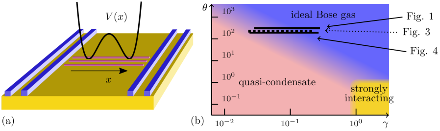
Figure 2: (a) The atom chip setup with the four wires (blue) creating the longitudinal potential and the three wires (red) creating the strong transverse confinement. (b) Position of our three data sets in the thermal equilibrium phase diagram of the Lieb-Liniger gas with $\gamma=mg/(\hbar^{2}n)$ and $\theta=2\hbar^{2}k_{\rm B}T/(mg^{2})$ phasediag . At the center of the cloud $\gamma$ is of order $10^{-2}$, but it increases in the wings as the density decreases; we display the segments $[\gamma_{\rm min},\gamma_{\rm min}/10]$ corresponding to a local density $n(x)$ not smaller than a tenth of the maximal density in the cloud. The asymptotic regimes of the Lieb-Liniger gas, separated by smooth crossovers, are shown in colors. Our data sets lie at the crossover between the quasicondensate and the ideal Bose gas (IBG) regimes.

The atom chip. Our experimental setup is described in detail in Ref. these-Aisling . ⁸⁷Rb atoms are confined in a magnetic trap produced by microwires deposited on the surface of a chip. The transverse confinement is provided by three 1.3 mm long parallel wires (red wires in Fig. 2), which carry AC currents modulated at 400 kHz: atoms are guided along $x$, at a distance of 12 $\mu$m above the central wire, with a transverse frequency $\omega_{\perp}$ which lies between 5 and 8 kHz. The modulation technique permits an independent control of the longitudinal potential $V(x)$, which is realized by two pairs of wires perpendicular to $x$, running DC current (blue wires in Fig. 2). The atomic cloud is far from those wires, in a region where $V(x)$ is well approximated by its Taylor expansion at small $x$. By tuning the currents in the four wires, we effectively control the coefficients of the $x$, $x^{2}$, $x^{3}$ and $x^{4}$ terms in that expansion: we can thus produce harmonic potentials, but also double-well potentials.

Using radio-frequency evaporative cooling we produce cold atomic clouds in the 1d regime, with a typical energy per atom smaller than the transverse energy gap: the temperature and chemical potential fulfill $k_{\rm B}T,\mu<\hbar\omega_{\perp}$. The gas is then well described by the 1d model (1), with the effective 1d repulsion strength $g=2\hbar a\omega_{\perp}$ olshanii_LL where the 3d scattering length of ${}^{87}{\rm Rb}$ is $a=5.3\,{\rm nm}$, and the mass is $m=1.43\times 10^{-25}$kg. Moreover the lengthscale on which $n(x)$ varies is much larger than microscopic lengths —the phase correlation length at thermal equilibrium, which is the largest microscopic length in the quasicondensate regime, is of order $n\hbar^{2}/(mk_{\rm B}T)$ Castin-Extension-2003 ; Cazalilla-Bosonizing-2004 , typically $0.1\,\mu$m for our clouds— so the hydrodynamic description applies. At equilibrium, the latter is equivalent to the Local Density Approximation (LDA), and the local properties of the gas are parametrized by the dimensionless repulsion strength $\gamma=mg/(\hbar^{2}n)$ and the dimensionless temperature $\theta=2\hbar^{2}k_{\rm B}T/(mg^{2})$ phasediag . The range $(\gamma,\theta)$ explored by our data sets is displayed in Fig. 2.(b). In this Letter we analyze the density profiles $n(x)$, which we measure using absorption images these-Aisling , averaging over typically ten images, with a pixel size of $1.74~{}\mu$m in the atomic plane.

The Yang-Yang initial profile. We start by trapping a cloud of $N=4600\pm 100$ atoms, with $\omega_{\perp}=2\pi\times(7.75\pm 0.02)\,{\rm kHz}$, in a harmonic potential $V(x)=m\omega_{\parallel}^{2}x^{2}/2$ with $\omega_{\parallel}=2\pi\times(8.8\pm 0.04)\,{\rm Hz}$, and measure its density profile (Fig. 1.(ii)). To evaluate the temperature of the cloud, we fit the experimental profile with the one predicted by the Yang-Yang equation of state yangyang ; Amerongen-Yang-2008 ; Jacqmin-Sub-Poissonian-2011 ; Volger-Thermodynamics-2013 , relying on LDA and on the assumption that the cloud is at thermal equilibrium; we find $T=(0.43\pm 0.013)\,\mu{\rm K}$. This gives $\theta=(3.5\pm 0.1)\times 10^{2}$, while the interaction parameter is $\gamma=(2.8\pm 0.1)\times 10^{-2}$ at the center.

As the density varies from the center of the cloud to the wings, the gas locally explores several regimes phasediag , from quasicondensate to highly degenerate Ideal Bose Gas (IBG) to non-degenerate IBG, see Fig. 2(b). The Yang-Yang equation of state yangyang is exact in the entire phase diagram of the Lieb-Liniger model, and thus faithfully describes the density profile within LDA. We stress that this is the most natural and powerful method to describe the initial state of the gas Amerongen-Yang-2008 ; Jacqmin-Sub-Poissonian-2011 ; Volger-Thermodynamics-2013 , and that no simpler approximate theory SMalternate can account for the whole initial density profile, see Fig. 1(ii). The Gross-Pitaevskii (GP) theory works in the central part—because it is close to the quasicondensate regime—, but not in the wings. The opposite is true for the IBG model: it correctly describes the wings, but not the center of the cloud—the chemical potential is positive in the center, so the density diverges in the IBG—. The classical field theory captures the quasicondensation transition for gases deep in the weakly interacting regime but it fails to reproduce faithfully the wings of our cloud since the latter are not highly degenerate.

Expansion from harmonic trap: agreement with both GHD and CHD.  At $t=0$, we suddenly switch off the longitudinal harmonic potential $V(x)$, and let the cloud expand freely in 1d. We measure the in situ profiles at times $t=10,20,30$ and 40 ms, see Fig. 1(i).

Two theories are able to give predictions for the expansion starting from the locally thermal initial state. One is GHD, presented above, where the full distribution of quasi-particles $\rho(x,v)$ is evolved in time footnote3 . The other is the conventional hydrodynamics (CHD) of the gas which, contrary to GHD, assumes that all local fluid cells are at thermal equilibrium, and keeps track only of three quantities that entirely describe the local state of the gas: the density $n(x)$, the fluid velocity $u(x)$, and the internal energy $e(x)$ SMalternate . We calculate the evolution of the density profile with both theories, and find that both of them are in excellent agreement with the experimental data, see Fig. 1(iii) for the result at $t=30$ ms.

GHD and CHD thus appear to be indistinguishable in that situation, at least for the expansion times that we probe here. We attribute this coincidence to the initial harmonic potential, which is very special. In this case it is simple to see that the GHD and CHD predictions coincide in the ideal Bose gas regime, and they can be shown to stay relatively near even beyond that regime SMharmonic .

Figure 3: (i) Longitudinal expansion of a cloud of $N=6300\pm 200$ atoms initially trapped in a double-well potential, compared with GHD. (ii) Even though the initial state is the same for GHD and CHD, both theories clearly differ at later times. CHD wrongly predicts the formation of two large density waves. The error bar shown at the center at $t=40$ms corresponds to a 68% confidence interval, and is representative for all data sets.

Discussion: GHD vs. CHD.  We wish to identify a setup where the theoretical predictions of both theories clearly differ, in order to experimentally discriminate between them. This will be the case if GHD predicts, for some time $t$ and at some position $x$, that the distribution of rapidities $\rho(x,v)$ will differ strongly from a thermal equilibrium one.

Such a situation occurs during the expansion of a cloud that initially has two well separated density peaks (Fig. 3). The reason can be captured by the following argument. The fluid cells $[x,x+\delta x]$ that are around either of the two peaks contain more quasi-particles, including quasi-particles of large rapidities, than the fluid cells near the center at $x=0$. Under time-evolution, the quasi-particles from the left peak that have a large positive rapidity $+u$ soon meet the ones coming from the right peak that have a large negative rapidity $-u$, around $x=0$. Then, the distribution of rapidities near $x=0$ is double-peaked, with maxima at $v\simeq\pm u$, so it is clearly very far from a thermal equilibrium distribution, which would be single-peaked. This phenomenon is obvious for non-interacting particles, Eq. (2) reducing to the standard Liouville equation, and GHD calculations indicate that this is true also for interacting particles ghd_qnc ; SMphasespace .

Expansion from a double-well.  To realize the above scenario, we prepare a cloud of $N=6300\pm 200$ atoms, with $\omega_{\perp}=2\pi\times(8.1\pm 0.03)\,{\rm kHz}$, at thermal equilibrium in a longitudinal double-well potential $V(x)$, such that the atomic density presents two well separated peaks, the peak density corresponding to $\gamma=(2.45\pm 0.07)\times 10^{-2}$. Then at $t=0$ we suddenly switch off the potential $V(x)$ and measure the in situ profiles at time $t=10$, $25$, $40$, $55\,{\rm ms}$ (Fig. 3).

To compare with theoretical predictions, we need to know the initial temperature $T$ of the cloud. However we cannot estimate $T$ from fitting the initial density profile $n_{0}(x)$ with the Yang-Yang equation of state and LDA because we do not have a good knowledge of the initial potential $V(x)$ that we create on the chip. Instead, we proceed as follows. First we postulate an initial temperature $T$ and construct the initial rapidity distribution $\rho_{T}(x,v)$ such that, for a given $x$, $\rho_{T}(x,v)$ is the thermal equilibrium rapidity distribution of Yang-Yang yangyang at temperature $T$ and density $n_{0}(x)$. We then evolve $\rho_{T}(x,v)$ using GHD and compute $n_{T}(x,t)$. While, by construction, $n_{T}(x,0)=n_{0}(x)$, $n_{T}(x,t)$ may differ from the data at later times. We repeat this procedure for several initial temperatures and we select the value of $T$ whose time evolution is in best agreement with the data SMprocedure . We obtain $T\simeq 0.3\,\mu{\rm K}$, corresponding to $\theta\simeq 2\times 10^{2}$, see Fig. 2(b).

The comparison between the expansion data and GHD is shown in Fig. 3(i); the agreement is excellent. We also simulate the time-evolution of the cloud with CHD, for the exact same initial state. As we expected, expanding from a double-well potential reveals a clear difference between CHD and GHD, see Fig. 3(ii). Two large density waves emerge in CHD and large gradients develop, eventually leading to shocks ddky , features which are not seen in GHD SMphasespace .

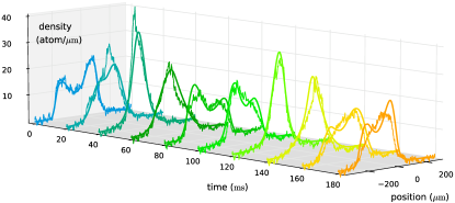
Figure 4: Quench from double-well to harmonic potential, compared to the GHD prediction, with an atomic cloud that contains $N=3500\pm 140$ atoms initially. The main features of the experimental data are well reproduced by GHD. One experimental effect, not modeled in GHD, that appears to be particularly important, are the three-body losses: after 180 ms, the number of atoms drops by approximately $15\%$.

Quench from double-well to harmonic potential. Finally, we trap $N=3500\pm 140$ atoms, with $\omega_{\perp}=2\pi\times(5.4\pm 0.02)\,{\rm kHz}$, in a double-well potential, and we study the evolution of the cloud after suddenly switching off the double-well and replacing it by a harmonic potential of frequency $\omega_{\parallel}=2\pi\times(6.5\pm 0.03)\,{\rm Hz}$. We measure the in situ profiles at time $t=0,20,40,\dots,180$ ms, see Fig. 4. The initial peak density corresponds to $\gamma=(2.13\pm 0.07)\times 10^{-2}$. To estimate the temperature of the cloud, we proceed as in the previous case SMprocedure ; we find $T\simeq 0.15\,\mu{\rm K}$, corresponding to $\theta\simeq 2.2\times 10^{2}$ (Fig. 2(b)).

This quench protocol mimics the famous quantum Newton’s Cradle experiment qnc —see also Refs. qnc2 ; qnc3 for recent realizations—, which is realized here in a weakly interacting gas. Exactly like in the previous paragraph, this is a situation where GHD predicts the appearance of non-thermal rapidity distributions ghd_qnc ; SMperiodicity , and must therefore differ strongly from CHD. In fact, we have observed that CHD develops a shock at short times (around $t\simeq 30$ ms), so it is simply unable to give any prediction for the whole evolution time investigated experimentally footnote2 .

Importantly, the motion is not periodic, contrary to what would be seen purely in the IBG or in the strongly interacting fermionized regime. Nevertheless, the motion of the cloud preserves an approximate periodicity, with a period close to, but slightly longer than, $2\pi/\omega_{\parallel}$ SMperiodicity (of course, if the cloud was symmetric under $x\rightarrow-x$, the period would be divided by two). At a quarter of the period —and three quarters of the period—, the density distribution shows a single thin peak located near $x=0$. We find good agreement with the GHD predictions, with the initial temperature $T$ as the only free parameter SMprocedure . However, experimental effects not taken into account by the GHD equations (2) appear to be more important in this setup than in the previous ones of Figs. 1-3, where shorter times were probed. For instance, the number of atoms $N$ is not constant in our experimental setup: it decreases with time and drops by approximately $15\%$ after $180$ ms, probably because of three-body losses which occur at large density. This might partially explain the difference between the experimental density profile and the GHD one. We also suspect the small residual roughness of the potential $V(x)$ of affecting the experimental profiles.

Conclusion. The results presented in this Letter are the first experimental check of the validity of GHD for 1d integrable quantum systems. We have shown that GHD —which predicts the time evolution of the distribution of rapidities— accurately captures the motion of 1d cold bosonic clouds made of $N\sim 10^{3}$ atoms, on time scales of up to $\sim 0.2$ seconds. We probed situations where the GHD predictions significantly differ from the ones of the conventional hydrodynamic approach, even at short times. We stress that GHD is applicable to all regimes of the 1d Bose gas, and it would therefore be particularly interesting to probe the strongly interacting regime. More generally, GHD is applicable to all Bethe Ansatz solvable models, including multicomponent mixtures of fermions and bosons with symmetric interactions Yang1967 ; sutherland ; gaudin ; batchelor , so it would be very exciting to use it to describe the dynamics of more complex gases which can be realized in experimental setups different from ours whitlock ; fallani .

Supplemental Material for “Generalized Hydrodynamics on an Atom Chip”

I Regimes of the Lieb-Liniger gas at thermal equilibrium

Properties of the Lieb-Liniger gas at thermal equilibrium have been studied extensively. The gas at thermal equilibrium is entirely parametrized by the dimensionless parameters $\gamma$ and $\theta$. Three main regimes have been identified, which correspond to different asymptotic value of the normalized zero-distance two-body correlation function $g^{(2)}(0)$ phasediag . The region in the ($\gamma,\theta$) plane corresponding to $\gamma\ll 1$ and $\theta\ll\gamma^{-3/2}$ is that of the quasicondensate regime. In this regime, correlations between particles are small and $g^{(2)}(0)\simeq 1$. Thus locally, the gas ressembles a Bose-Einstein condensate, although quantum and thermal fluctuations associated to long wavelength phonons prevent true long range order. The region $\theta\gg\rm{max}(1,\gamma^{-3/2})$ is that of the ideal Bose gas regime, characterized by $g^{(2)}(0)\simeq 2$. In this regime repulsive interactions are not strong enough to prevent the thermally activated large density fluctuations associated to the bosonic bunching phenomenon. Finally, the region $\theta\ll 1$ and $\gamma\gg 1$ is that of the strongly interacting regime, also called Tonks-Girardeau or fermionized regime. There, interactions are strong enough to almost prevent two atoms to sit at the same position so that $g^{(2)}(0)\ll 1$.

The above-mentioned regimes are all separated by smooth crossovers. Quantitative values for the position of these transitions depend on the quantity that is considered and on the criteria used. One possible criterion to locate the transition from the IBG to qBEC regime is the condition $\mu=0$, where $\mu$ is the chemical potential: in the IBG regime, $\mu<0$ while $\mu>0$ in the qBEC regime ($\mu\simeq gn$ in the qBEC regime). In Fig. 5, we plot the line $\mu=0$, found using the Yang-Yang equation of state. This line follows the expected scaling $\theta\propto\gamma^{-3/2}$ of the crossover between the IBG and the qBEC regime. It lies however substantially above the line $\theta=\gamma^{-3/2}$ phasediag .

The IBG regime can be divided into two subregimes: the highly non-degenerate regime corresponding to $\theta\gg\gamma^{-1/2}$ and the highly degenerate regime corresponding to $\gamma^{-3/2}\ll\theta\gg\gamma^{-1/2}$. The crossover between these two subregimes is very wide and in fig. 5, we signal this transition with the line corresponding to $n\lambda_{dB}=1$, where $\lambda_{dB}=\hbar/\sqrt{2\pi mk_{B}T}$ is the de Broglie wavelength.

Figure 5: Position of the three sets of data shown in the text in the $(\gamma,\theta)$ space. The thin solid line is the line corresponding to a vanishing chemical potential, computed using Yang-Yang equation of state, which indicates the crossover from the Ideal Bose gas to the quasi-condensate. The dashed line is the line $n\lambda_{\rm{dB}}=1$ which indicates the crossover from a non-degenerate to a highly degenerate gas. The horizontal fat lines correspond to the experimental data investigated in the main text (from top to bottom data of Fig.1, data of Fig.3 and data of Fig. 4).

II Approximate theories that we compare to GHD

II.1 Conventional hydrodynamics based on Yang-Yang thermodynamics (or Thermodynamic Bethe Ansatz)

What we call ‘conventional’ hydrodynamics (CHD) in the main text is simply the Euler equations that hold in normal fluids that are locally at thermal equilibrium, that govern the variation of the particle density $n(x,t)$, the fluid velocity $u(x,t)$, and the internal energy per particle $e(x,t)$:

$$\left\{\begin{array}[]{rcl}\partial_{t}n+\partial_{x}(un)&=&0\\ \partial_{t}u+u\partial_{x}u+\frac{1}{mn}\partial_{x}P&=&-\frac{1}{m}\partial_{x}V\\ \partial_{t}e+u\partial_{x}e+\frac{P}{n}\partial_{x}u&=&0.\end{array}\right.$$ (3)

Here $P(n,e)$ is the pressure, which is given by the equation of state of the fluid. One can put these three equations in a form that expresses conservation of mass, momentum—broken by the external potential $V(x)$—, and energy,

$$\left\{\begin{array}[]{rcl}\partial_{t}n+\partial_{x}(un)&=&0\\ \partial_{t}(mnu)+\partial_{x}(u(mnu)+P)&=&-n\partial_{x}V\\ \partial_{t}(n\frac{mu^{2}}{2}+ne+nV)+\partial_{x}(u(n\frac{mu^{2}}{2}+ne+nV)+uP)&=&0.\end{array}\right.$$ (4)

These are the evolution equations we solve to obtain the Conventional HydroDynamics (CHD) curves in the main text. The pressure $P(n,e)$ is obtained from the thermodynamic Bethe Ansatz, also known as the Yang-Yang equation of state yangyang .

One convenient way to calculate the pressure is to observe that it is the momentum current, and then to use the formula from ghd for the latter,

$$P\,=\,\frac{m^{2}}{\hbar}\int\frac{dv}{2\pi}v\,\nu(v)\,v^{\rm dr}.$$ (5)

Here $\nu(v)\in[0,1]$ is the occupation function, which, for the thermal Gibbs state at inverse temperature $\beta=1/(k_{\rm B}T)$, satisfies the integral equation of Yang and Yang yangyang ,

$$\beta\frac{mv^{2}}{2}\,=\,\log\left[\frac{1-\nu(v)}{\nu(v)}\right]\,-\,\int\frac{dw}{2\pi}K(v-w)\log\left[1-\nu(w)\right],$$ (6)

where $K(v-w)=\frac{2(v-w)/\hbar}{(g/\hbar)^{2}+(v-w)^{2}}$ is the differential scattering phase, or Lieb-Liniger kernel. The superscript ’dr’ in (5) stands for ’dressing’, and is defined as follows for a function $f(v)$,

$$f^{\rm dr}(v)\,=\,f(v)+\int\frac{dw}{2\pi}K(v-w)\nu(w)f^{{\rm dr}}(w)$$ (7)

(and by a slight abuse of notation, we write $v^{\rm dr}$ for ${\rm id}^{\rm dr}(v)$ where ${\rm id}(v)=v$ is the identity function). The occupation function $\nu(v)$ and the distribution $\rho(v)$ used in the main text are related by

$$\rho(v)=\frac{m}{2\pi\hbar}\,\nu(v)\,1^{\rm dr}(v)$$ (8)

where $1(v)=1$. The function $\nu(v)$ gives the occupation fraction of the rapidities, which are the fermionic quantities defining a Bethe-Anstaz eigenstate yangyang .

II.2 Gross-Pitaevskii approach

The Gross-Pitaevskii description (GP) assumes that the gas is Bose-condensed : all the atoms are in the same single-particle wave function $\psi(x)$. It describes a Bose gas at zero temperature in the limit of weak repulsion $\gamma\rightarrow 0$, as long as their extension is much smaller than $\xi e^{\pi/\sqrt{\gamma}}$, where $\xi=\hbar/\sqrt{m\rho}$ is the healing length. The latter condition, usually fulfilled in experiment with weakly interacting gases, ensures that quantum fluctuations do not break long-range order. At equilibrium the wavefunction $\psi$ obeys

$$\mu\psi=\,\left(-\frac{\hbar^{2}}{2m}\partial_{x}^{2}+g|\psi|^{2}+V(x)\right)\psi$$ (9)

where $\mu$ is the chemical potential. After modification of the potential, the time evolution of $\psi$ is given by the Gross-Pitaevskii equation

$$i\hbar\partial_{t}\psi\,=\,\left(-\frac{\hbar^{2}}{2m}\partial_{x}^{2}+g|\psi|^{2}+V(x)\right)\psi.$$ (10)

Here $\psi(x,t)$ is the wavefunction of the condensate at time $t$, normalized such that

$$\int dx|\psi(x,t)|^{2}\,=\,N.$$ (11)

Separating the phase and the amplitude of the wavefunction of the condensate,

$$\psi(x,t)\,=\,\sqrt{n(x,t)}e^{i\varphi(x,t)},$$ (12)

and introducing the velocity field $u=\frac{\hbar}{m}\partial_{x}\varphi$, one gets GP in Madelung form,

$$\begin{array}[]{rcl}\partial_{t}n+\partial_{x}(un)&=&0\\ \partial_{t}u+u\partial_{x}u&=&-\frac{1}{m}\partial_{x}\left[gn+V(x)-\frac{\hbar^{2}}{2m}\frac{\partial_{x}^{2}\sqrt{n}}{\sqrt{n}}\right].\end{array}$$ (13)

The first equation expresses conservation of mass, the second is the Euler equation for a fluid with the equation of state $\mu=gn$ in an external potential $V(x)$, with an additional quantum pressure term $\frac{\hbar^{2}}{2m}\frac{\partial_{x}^{2}\sqrt{n}}{\sqrt{n}}$. In the Euler limit of long wavelengths for density variations, the quantum pressure term can be neglected. Then Eq. (13) reduces to the Euler equation with a pressure term $P=gn^{2}/2$, which is indeed the pressure of a condensate or a quasicondensate. Note however that the GP equation goes beyond this Euler limit of long wavelength variation of $\psi$. For instance, it would capture correctly the “quantum Newton craddle” experiment presented in the main text, for a weakly interacting cloud at $T=0$. At the “collision-time” where the two initial clouds are on top of each other, GP predicts fast oscillations of the density reflecting interference phenomena. Of course such fast oscillations, which, in terms of Bethe-Ansatz states, would imply interference between different states (of very similar quasi-momentum distribution), is not accounted for by GHD. However we expect that predictions of GHD (for a weakly interacting gas at $T=0$) would coincide with the GP ones, if one perform a spatial coarse-grained approximation of the GP solution, smearing out the interference fringes. It is an open question under which precise conditions and coarse-graining procedure the predictions of GHD coincide with the coarse-grained GP predictions.

II.3 The classical field approximation

In the domain characterized by $\gamma^{-1}\ll\theta\ll\gamma^{-2}$, the typical occupation number of the relevant modes (either the one-particle states for $\theta\gg\gamma^{-3/2}$, or the Bogolioubov collective modes for $\theta\ll\gamma^{-3/2}$) is much larger than one: in particular the correlation functions are mainly dominated by the contribution of highly populated modes. In such a condition, a theory that neglects the quantification of the atomic field $\hat{\psi}$ and treat it as a complex classical field —or equivalently, that considers statistical fluctuation of the condensate’s single-particle wave function— is expected to provide the relevant physics. This is the so-called classical field approximation Castin-coherence-2000 . At thermal equilibrium the complex field $\psi(x)$ obeys the probability distribution

$$P(\{\psi(x)\})=Z^{-1}e^{-\beta\int dx(\hbar^{2}/(2m)|\partial_{x}\psi|^{2}+g/2|\psi|^{4}+(V(x)-\mu)|\psi|^{2})},$$ (14)

where $\beta=1/(k_{B}T)$, $\mu$ is the chemical potential, and the partition function $Z$ ensures the correct normalization. At sufficiently shallow confining potential, a local density approximation is valid and the external potential $V(x)$ is not very relevant. Note that while two parameters are required to describe a Lieb-Liniger gas, only one parameter, which can be taken as $\eta=\mu(\hbar^{2}/(mg^{2}k_{B}^{2}T^{2}))^{1/3}$ in terms of the temperature and chemical potential, is sufficient to characterize the classical field, providing lengths and densities are correctly rescaled Castin-coherence-2000 ; isabelle_twobody . One way of sampling the field $\psi$ according to Eq. (14) is to numerically evolve $\psi$ under a stochastic differential equation.

In contrast to the GP approach above, the classical field takes into account thermal fluctuations in the system. In particular it captures the quasicondensation crossover, which occurs, for $\gamma\ll 1$, around the line $\theta=\gamma^{-3/2}$, although very large values of $\theta$ are required for an accurate description of the gas jacqmin-momentum . On the other hand, it ignores the quantification of atoms. This leads to an overestimation of the population in high energy modes: within CF theory the mode population is $k_{B}T/\epsilon_{\nu}$, regardless of the mode energy $\epsilon_{\nu}$, a value much larger, for modes of energy $\epsilon_{k}\gg k_{B}T$, than the expected exponential behavior $e^{-\epsilon_{k}/(k_{B}T)}$ (this is a similar phenomenon as that of the well-known UV catastrophe of thermal ensembles of electromagnetic fields). This explains why the equilibrium profile predicted by the classical field model strongly overestimate the wings of the atomic clouds, see Fig. 1(ii) in the main text. We are aware of refined theories, based on classical field, that include a well-chosen cutoff above which the excitations are treated as a quantum gas, see Cockburn-comparison-2011 ; Blakie and references therein. They permit to reproduce the equilibrium density profiles of trapped weakly interacting gases Cockburn-comparison-2011 . However, expanding such theories to time-dependent problems is a priori not trivial. We also think that, in the same way as Yang-Yang thermodynamics offers a much more powerful, reliable and elegant way of describing the equilibrium profiles Amerongen-Yang-2008 ; Jacqmin-Sub-Poissonian-2011 ; Volger-Thermodynamics-2013 , GHD would supersede complicated and ad-hoc theories based on the classical field approximation.

III Relation between GHD and CHD for an expansion from a harmonic potential

As we observed in the main text, the one-dimensional expansion of the gas starting from a state where it is confined by harmonic potential is well described both by GHD and CHD. This is surprising, as GHD takes into account infinitely many conservation laws, while CHD only takes into account three: mass, momentum and energy. Of course, the initial state is, in both cases, obtained by a Gibbs local density approximation, according to which in every mesoscopic cell the gas is a Gibbs state, thermalized with respect to the energy and number of particles (with zero average momentum). Nevertheless, one generically expects that under the GHD evolution, other conservation laws become involved, the fluid being, after some time, locally a generalized Gibbs ensemble – involving higher conserved charges – instead of a Gibbs ensemble.

There are two limits where one can show that the GHD evolution is, in fact, the same as the CHD evolution.

The first is the zero-temperature limit. It was shown in Ref. ddky that if the initial state is at zero temperature, where, in every cell $x$, the quasi-particle occupation function $\nu(x,v)$ takes the value 1 on an interval $v\in[v_{l}(x),v_{r}(x)]$ and 0 elsewhere, then, at least for small enough times, a GHD evolution is completely equivalent to a CHD evolution, and the state stays at zero temperature. This holds from any initial potential, harmonic or not. The equivalence between the evolutions breaks down when in CHD shocks develop; in GHD, large gradients are temporary, and the fluid passes to a higher-dimensional space of states afforded by the higher conservation laws.

The other limit is that of the free gases - either the ideal Fermi gas (at strong coupling) or the ideal Bose gas (IBG) (at large temperatures). Let us consider the latter, as it is more relevant to the present experiment. In the free limit, the effective velocity becomes equal to the velocity, and the initial fluid’s Bosonic occupation function $\tilde{\nu}(x,v)$ (note that this is related to, but not the same as, the quasi-particle – or fermionic – occupation function $\nu(x,v)$) is of the form

$$\tilde{\nu}(x,v)=\frac{1}{e^{(mv^{2}/2+m\omega_{\parallel}^{2}x^{2}/2-\mu)/T}-1}.$$ (15)

The GHD evolution during the expansion is very simple,

$$\partial_{t}\tilde{\nu}+v\partial_{x}\tilde{\nu}=0,$$ (16)

and thus the solution is obtained as

$$\tilde{\nu}(x,t,v)=\frac{1}{e^{(mv^{2}/2+m\omega_{\parallel}^{2}(x-vt)^{2}/2-\mu)/T}-1}=\frac{1}{e^{(m(v-u(x,t))^{2}/2)(1+\omega_{\parallel}^{2}t^{2})/T}e^{(m\omega_{\parallel}^{2}/(1+\omega_{\parallel}^{2}t^{2})\,x^{2}/2-\mu)/T}-1},$$ (17)

where $u(x,t)=\omega_{\parallel}^{2}/(1+\omega_{\parallel}^{2}t^{2})\,xt$. Eq. (17) shows that the distribution of $v$ at a given $x$ is that of a Gibbs ensemble for a gas whose center of mass moves at velocity $u(x,t)$. Hence, all currents obtained after GHD evolution are evaluated within Gibbs states, completely determined by the first three conserved densities. Therefore, it is sufficient to restrict to the evolution described by the first three conservation laws, and we recover CHD.

These two limits, however, only partially explain the observation we have made: the parameters of the experiment, the full range of regimes covered by the gas (see Fig. 2b in the main text), imply that there are regions where the occupation function is both relatively far from the zero-temperature form (see typical initial quasi-particle occupation functions in section IV) and from the IBG form.

We provide below a calculation that shows that, more generally, one may expect the GHD solution to stay relatively near to CHD solution in an expansion from a harmonic potential, even away from the two limits described above. The main result is that under GHD evolution from a harmonic potential, the occupation function has the same asymptotics at large $v$, of the form $e^{-P(v)}$ with $P(v)$ a polynomial of degree 2, as that obtained from a CHD evolution. That is, the “wings” in quasi-momentum space are not drastically affected by the presence of higher conservation laws. Further, at finite $v$, the discrepancies must stay bounded. If the occupation function is near enough to the zero-temperature form, with a region relatively near to 1 at small velocities, surrounded by wings where it tends towards 0, then a combination of the zero-temperature result recalled above, and the asymptotic results derived below, suggests that indeed the GHD and CHD solutions should stay near. Typical initial occupation functions shown in section IV indeed have this form, and thus these arguments explain our observation.

In terms of the quasi-particle occupation function $\nu(v)$, related to the quasi-particle density $\rho(x,v)$ via (8), it turns out that Eq. (2b) in the main text becomes

$$\partial_{t}\nu+v^{\rm eff}\partial_{x}\nu=0.$$ (18)

The pseudoenergy $\epsilon$, defined via $\nu=1/(1+e^{\epsilon})$, hence satisfies the same equation,

$$\partial_{t}\epsilon+v^{\rm eff}\partial_{x}\epsilon=0.$$ (19)

In order to describe the macrostate, it is convenient to use the energy function $e(v)$, in terms of which the pseudoenergy can be expressed as the solution to the non-linear integral equation yangyang

$$\epsilon(v)=e(v)-\int\frac{dw}{2\pi}\,K(v-w)\log(1+e^{-\epsilon(w)}).$$ (20)

Like the quasi-particle density, the energy function $e(v)$, in GHD, becomes space-time dependent, and we can re-write (19) using (20). One can show that dy

$$(\partial_{t}e)^{\rm dr}+v^{\rm eff}(\partial_{x}e)^{\rm dr}=0$$ (21)

where the dressing operation is defined in (7). Note that the effective velocity (Eq. 2a in the main text) can be written as

$$v^{\rm eff}=v^{\rm dr}/1^{\rm dr}$$ (22)

where $v^{\rm dr}$ is the dressed of the function $v$ (the identity function), and $1^{\rm dr}$ is the dressed of the constant function 1 ($1^{\rm dr}$ and all dressed quantities are functions of $v$, as well as, of course, the space-time position $x,t$). Therefore, we have

$$(\partial_{t}e)^{\rm dr}+\frac{v^{\rm dr}}{1^{\rm dr}}(\partial_{x}e)^{\rm dr}=0$$ (23)

In the initial state, at $t=0$, for each position $x$ the state of the gas is given by the Gibbs ensemble, with a chemical potential $\mu-m\omega_{\parallel}^{2}x^{2}$ and a temperature $T$, and the energy function reduces to yangyang

$$e(x,0,v)=\frac{1}{T}\left(\frac{mv^{2}}{2}+\frac{m\omega_{\parallel}^{2}x^{2}}{2}-\mu\right).$$ (24)

We propose that an approximate solution to the evolution equation from a harmonic potential is of the form

$$e(x,t,v)\approx f(t)v^{2}+g(t)vx+h(t)x^{2}-\mu.$$ (25)

This approximate solution holds if the following condition is approximately satisfied,

$$(v^{\rm dr})^{2}\approx(v^{2})^{\rm dr}1^{\rm dr}.$$ (26)

Indeed inserting (25) in (21) gives

$$f^{\prime}(t)(v^{2})^{\rm dr}+g^{\prime}(t)v^{\rm dr}x+h^{\prime}(t)x^{2}1^{\rm dr}+g(t)(v^{\rm dr})^{2}/1^{\rm dr}+h(t)xv^{\rm dr}\approx 0$$ (27)

And so we have

$$h^{\prime}(t)=0,\quad g^{\prime}(t)=-h(t),\quad f^{\prime}(t)(v^{2})^{\rm dr}\approx-g(t)(v^{\rm dr})^{2}/1^{\rm dr}.$$ (28)

If the approximation (26) holds, then the last (approximate) equation becomes

$$f^{\prime}(t)\approx-g(t)$$ (29)

and we find

$$h(t)=a,\quad g(t)=b-at,\quad f(t)=c-bt+at^{2}/2.$$ (30)

The initial condition is satisfied, with $a=m\omega_{\parallel}^{2}/(2T)$, $b=0$ and $c=m/(2T)$.

We now note that the approximate solution (25) with (30) is exactly the form we would obtain (under (26)) from CHD: in all cells it is a boosted Gibbs state, completely determined by the mass, momentum and energy densities, hence we can restrict to these conservation laws. The validity of CHD thus reduced to the investigation of the validity of the approximation (26).

From (20), we see that $\epsilon(v)$ has the same leading large-$|v|$ asymptotics as $e(v)$. Hence, in states with power-law growing $e(v)$, the occupation function decays as an exponential of a power at large $|v|$. From the dressing operation (7), it is then clear that, in any such state, the dressed $f^{\rm dr}(v)$ of any function $f(v)$ has exactly the same asymptotic expansion in powers of $1/v$ up to powers $1/v^{2}$: the corrections coming from the occupation function are exponentially decaying, hence the main corrections come from integrating the differential scattering kernel around finite regions of the integration variable $w$ (the size of the finite region being controlled by the exponential decay of the occupation function). These give the power law $1/v^{2}$. That is, assuming $f^{\rm dr}(v)$ stays finite for finite values of $v$, we have

$$f^{\rm dr}(v)=f(v)+O(1/v^{2}).$$ (31)

Therefore

$$(v^{\rm dr})^{2}=(v^{2})^{\rm dr}1^{\rm dr}+O(1/v)$$ (32)

and the condition (26) is satisfied up to vanishing terms at large $v$. This fully justifies that the approximate solution (25) indeed holds as written, up to vanishing terms, and shows that CHD reproduces the correct non-vanishing large-$v$ asymptotics of $e(v)$, and thus (by a similar asymptotic analysis as above) of $\epsilon(v)$.

At small velocities, the effective velocity $v^{\rm eff}$ is different from $v$ due to transport within its local environment: for instance, a quasi-particle of bare velocity $v=0$ acquires a nonzero effective velocity $v^{\rm eff}\neq 0$ if its surrounding environment carries nonzero currents. However, these differences are bounded, and tend to be relatively small. Similar effects occur for the dressing of any function, and therefore the approximation (26) has an error that stays bounded at finite $v$.

Finally, we note from the above calculations and especially from (31) that the free evolution (with trivial dressing) generically (that is, in all situations where the occupation function decays at least exponentially) describes correctly the first three leading powers of the large-$v$ asymptotics of the source term $e(v)$ under the one-dimensional expansion (recall that in the case of the initial harmonic potential, the free evolution agrees with CHD, but that in general it does not). One could for instance consider an initial potential with higher powers, say up $x^{4}$. Then we see that an approximate solution of similar type, valid at large $v$, would have powers of $v$ up to $v^{4}$, with the coefficients of the powers $v^{2}$, $v^{3}$ and $v^{4}$ correctly described by a free evolution equation. This is definitely very far from a CHD solution, as powers of $v^{3}$ and $v^{4}$ are forbidden in CHD. That is, when starting from non-harmonic potentials, CHD does not describe the correct large-$v$ asymptotics of the distribution, hence is quite far for all $v$ – the maximal deviation for the function $e(v)$ is in fact is unbounded. It is these effects that are seen in section IV.

IV GHD vs. CHD: comparison of the phase-space occupation functions $\nu(x,v)$

Here we display the phase-space occupation $\nu(x,v)$ for the expansion from a double-well potential shown in Fig. 3 in the main text. At each $x$, the occupation function $\nu(v)$ is related to the density $\rho(v)$ used in the main text by Eq. (8). At thermal equilibrium, one can think of it as a Fermi distribution: at zero temperature, it is exactly a rectangular function, with support $[-2\sqrt{\frac{gn}{m}},2\sqrt{\frac{gn}{m}}]$ in the limit of weak repulsion. At finite temperature the two sides of the rectangle are rounded off. The GHD evolution equation can be written directly in terms of the occupation function $\nu(v)$, see Eq. (18).

On the phase-space pictures in Fig. 6, one clearly sees why CHD must differ from GHD. Indeed, initially the phase-space occupation is the equilibrium one at temperature $T=0.3\,\mu{\rm K}$, obtained from LDA in the double-well potential $V(x)$, see the main text. Because the atomic density increases near the two minima of the potential $V(x)$, the interval $[v_{1},v_{2}]$ in which the occupation function is close to $1$ is larger near these points. This results in the support of $\nu(x,t)$ looking like a peanut at $t=0$. By definition, the initial distribution is the same for GHD and CHD.

Generalized HydroDynamics (GHD):
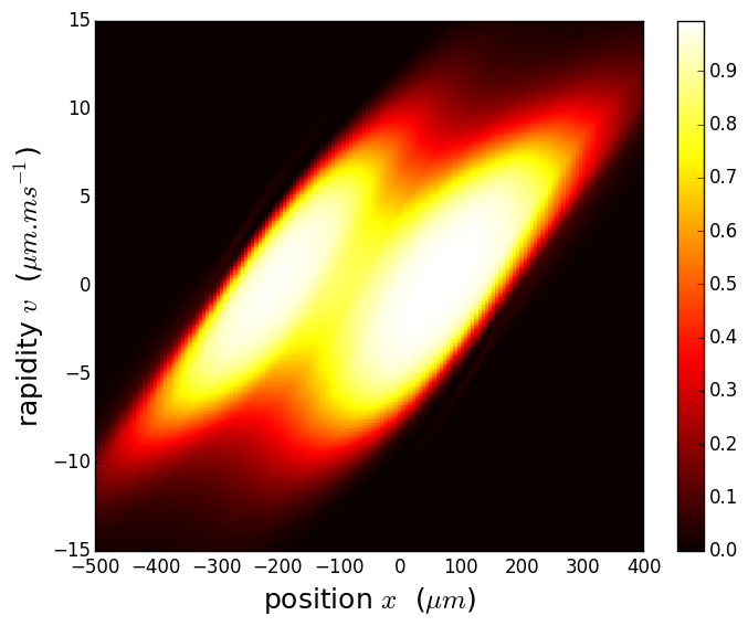
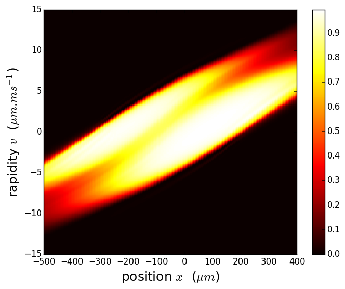
$t=0$	$t=25$ ms	$t=55$ ms
Conventional hydrodynamics (CHD):
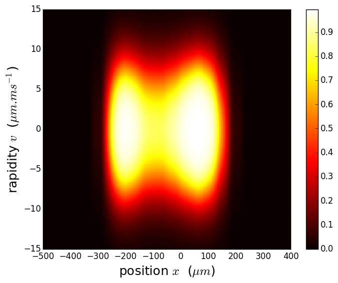
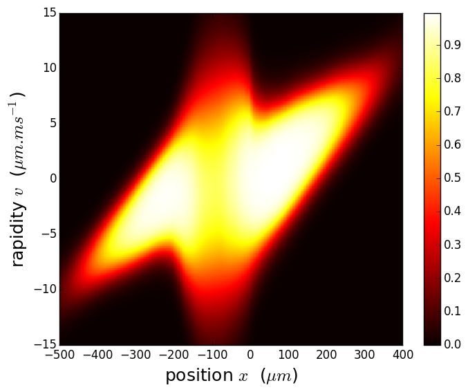
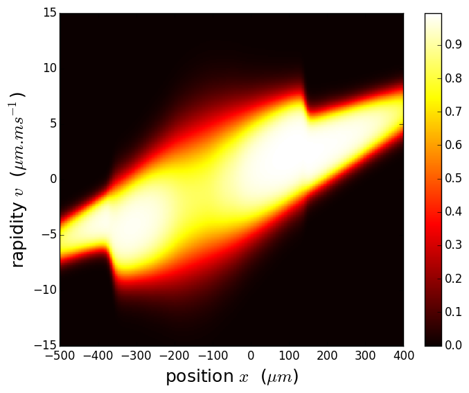
$t=0$	$t=25$ ms	$t=55$ ms

Figure 6: Phase-space occupation $\nu(x,v)$ at time $t$ for the parameters of Fig. 3 in the main text, simulated with GHD and CHD. Since CHD does not allow non-thermal local distributions of rapidities, we see that the distribution gets quickly distorted, compared to the GHD one. This results in the two in situ density profiles being clearly different, see Fig. 3 in the main text.

At later times, the distribution gets distorted. GHD predicts that the top of the support of $\nu(x,v)$ moves to the right, while the bottom of the support moves to the left. At $t\simeq 25$ ms we already see that, for a fixed $x$ in the central region around $x=0$, the occupation function $\nu(v)$ does not look like a thermal equilibrium distribution anymore: instead of being a rounded rectangular function, it is now a function that has two maxima. This gets worse as time increases: the distribution $\nu(v)$, for fixed position $x$, differs more and more from an equilibrium one.

CHD, on the contrary, enforces an equilibrium occupation function at all positions and all times. Therefore, it must differ significantly from GHD. Indeed, this is what we see in the phase-space occupation at $t=25$ ms, where the occupation function of CHD is distorted in the central region, compared to the GHD one, in order to maintain a thermal state. The discrepancy between GHD and CHD then keeps increases at later times.

The density profiles of Fig. 3 in the main text are obtained from these phase-space occupation function $\nu(x,\theta)$ by Eq. (8) and then integrating over all rapidities at fixed position $x$, $n(x)=\int\rho(x,v)dv$.

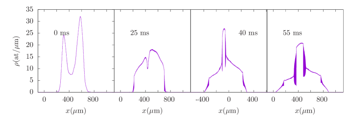
Figure 7: Expansion of a cloud whose initial density distribution is equal to that of the experimental data of Fig. 3 in the main text, according to the Gross-Pitaevskii equation. The evolution is very different from that observed experimentally, with the appearance of a central peak, not seen experimentally.

V Gross Pitaevskii predictions for expansion from a double well

We performed a Gross Pitaevskii calculation for the situation considered in Fig.3. In this calculation, the initial wavefunction is $\psi(x)=\sqrt{n_{0}(x)}$, where $n_{0}(x)$ is the initial experimental profile. We then evolve this initial profile according to the time-dependant Gross-Pitaevskii equation Eq. (10). The resulting time evolution, shown in Fig.(7), is very different from that observed experimentally. This indicates that thermal excitations initially present in the cloud play an important role in the time-evolution shown in Fig.3. Note that GHD calculations performed at a very low temperature are in agreement with these Gross-Pitaevskii calculations, provided fast oscillations shown in the Gross-Pitaevski profiles are averages out (see section VI).

VI Running the GHD simulation without good knowledge
of the initial potential $V(x)$

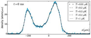
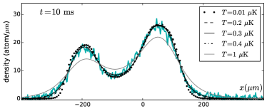
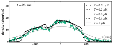
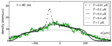
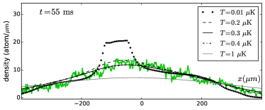
Figure 8: Comparison between the experimental data of Fig. 3 in the main text, and the GHD simulation assuming three different temperatures of the initial state. For Fig. 3 in the main text, we selected the results corresponding to $T=0.3\,\mu$K.

The creation of a double-well potential on the chip is experimentally tricky, and, as a result, we do not have a very good knowledge of this potential. It should be close to a polynomial potential of fourth degree, $V(x)\simeq\sum_{p=0}^{4}a_{p}x^{p}$, but we do not know the coefficients $a_{p}$. One could extract them from a fit, but then we would have $6$ adjustable parameters in total: the five coefficients $a_{p}$, and the temperature of the initial state.

On the other hand, the initial potential $V(x)$ is needed only to reconstruct the initial distribution $\rho(x,v)$. So, instead of trying to reconstruct first the potential $V(x)$ and then the initial distribution $\rho(x,v)$, we find it more satisfying to construct directly that distribution, assuming that it is given by a thermal Gibbs state in every fluid cell at position $x$. When we do that, there is a single adjustable parameter: the initial temperature, assumed to be initially homogeneous throughout the cloud.

We proceed as follows. First, we take a convolution of the experimental density at time $t=0$ with a gaussian, in order to get a smooth initial density profile $n(x)$. Then we fix arbitrarily a temperature $T$, and, assuming that the gas is locally at equilibrium at temperature $T$, we reconstruct the occupation function $\nu(x,\theta)$—or equivalently the distribution $\rho(x,\theta)$—using the Yang-Yang equation of state (6). Let us emphasize that, at this point, we have reconstructed a density profile, which corresponds to some potential $V_{T}(x)$, and the latter potential is not independent of the choice of the temperature $T$. What we then want, of course, is to identify the correct $T$ corresponding to the correct experimental $V(x)$ which, unfortunately, we do not know a priori. We then run the GHD simulation, which allows us to compute the density profiles at later times $t$. Those density profiles at later times depend on the initial state, therefore they depend on $T$.

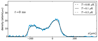
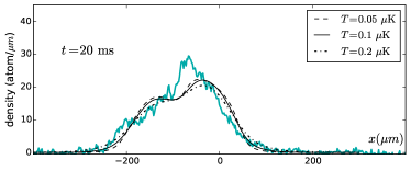
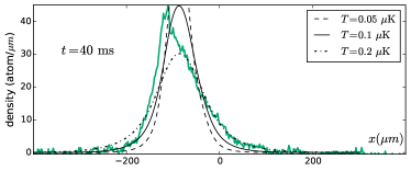
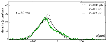
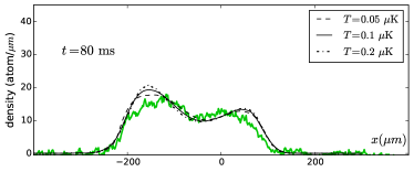
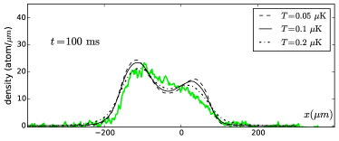
Figure 9: Comparison between the experimental data of Fig. 4 in the main text, and the GHD simulation assuming three different temperatures of the initial state. For Fig. 4 in the main text, we selected the results corresponding to $T=0.1\,\mu$K.

We do this for several values of the initial temperature $T$. In Fig. 8 we display the results for the data set shown in Fig. 3 in the main text, for initial temperatures $0.2\,\mu{\rm K}$, $0.3\,\mu{\rm K}$ and $0.4\,\mu{\rm K}$. We see that the results do not strongly dependent on the temperature. More quantitatively, for each $T$ we measure the mean distance between the experimental data and the GHD prediction defined as $\sqrt{\frac{1}{N_{\rm{data}}}\sum_{x,t}[n_{\rm data}(x,t)-n_{\rm GHD}(x,t)]^{2}}$, where the sum is done over all the data points for different positions $x$ and times $t$ and $N_{\rm{data}}$ is the total number of data points. For temperatures $T=0.01,0.2,0.25,0.3,0.35,0.4,1\,\mu{\rm K}$, we find that the distance is respectively $1.21,0.66,0.62,0.61,0.64,0.63,1.26$ (atom/$\mu$m). In the main text, we have selected the GHD results with $T=0.3\,\mu{\rm K}$, corresponding to the minimum of that distance for the set of temperatures simulated.

We have proceeded in the same way for the quench from a double-well to harmonic potential, corresponding to the data set shown in Fig. 4 in the main text. In Fig. 9 we display the GHD curves for initial temperatures $0.05\,\mu{\rm K}$, $0.1\,\mu{\rm K}$ and $0.2\,\mu{\rm K}$, up to time $t=100$ ms after the quench. We have performed the GHD simulation for temperatures For temperatures $T=0.05,0.75,0.1,0.125,0.15,0.2,0.3\,\mu{\rm K}$, we find that the mean distance is respectively $2.69,2.19,1.88,1.71,1.64,1.72,2.08$ (atom/$\mu$m). In the main text, we have selected the GHD results with $T=0.15\,\mu{\rm K}$, corresponding to the minimum of that distance for the set of temperatures simulated.

VII Approximate periodicity of the GHD solution for the quench from double-well to harmonic potential

In Fig. 10 we display the phase-space occupation $\nu(x,v)$ for the quench from double-well to harmonic potential, corresponding to the GHD data shown in Fig. 4 in the main text. We recall that $\nu(x,v)$ is the phase-space occupation, and that it is related to the phase-space density used in the main text by Eq. (8). One can roughly think of $\nu(x,v)$ as a Fermi dstribution, see App. III above. The GHD evolution equation can be written directly in terms of the occupation function $\nu(v)$, see Eq. (18).

It is clear from these plots that, after one period of the harmonic trap (the period is 154 ms), the distribution is only approximately similar to the initial one. So, even though our atomic clouds are weakly interacting, the behavior that is predicted by GHD is clearly different from the one of non-interacting particles, since the latter would be exactly periodic.

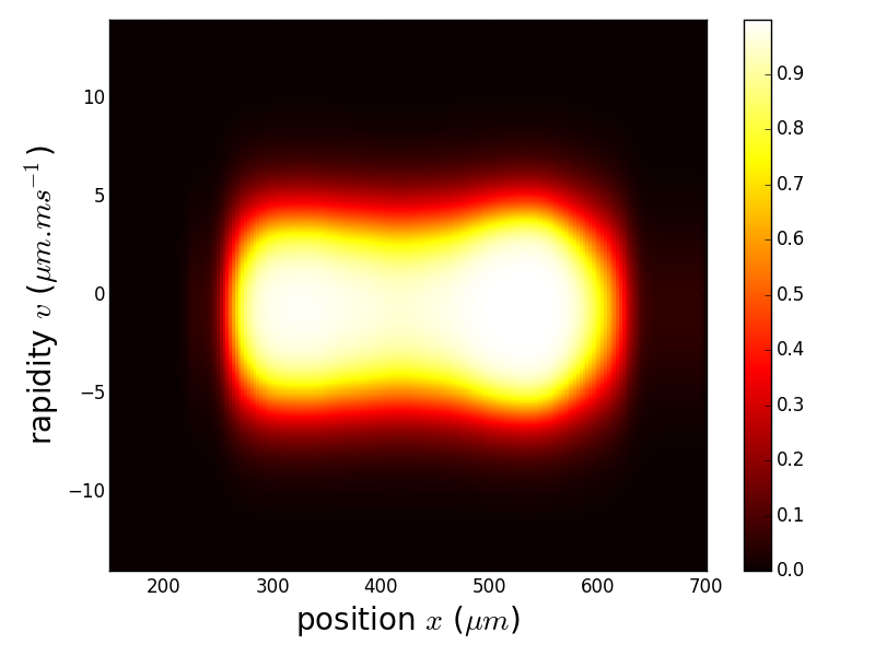
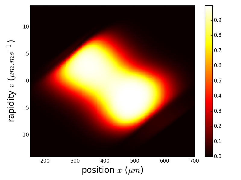
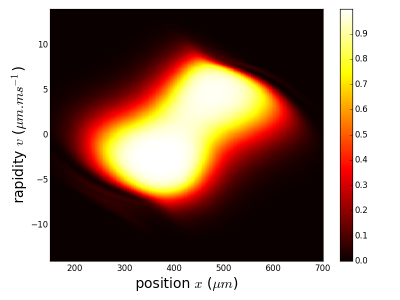
$t=0$	$t=20$ ms	$t=40$ ms	$t=60$ ms
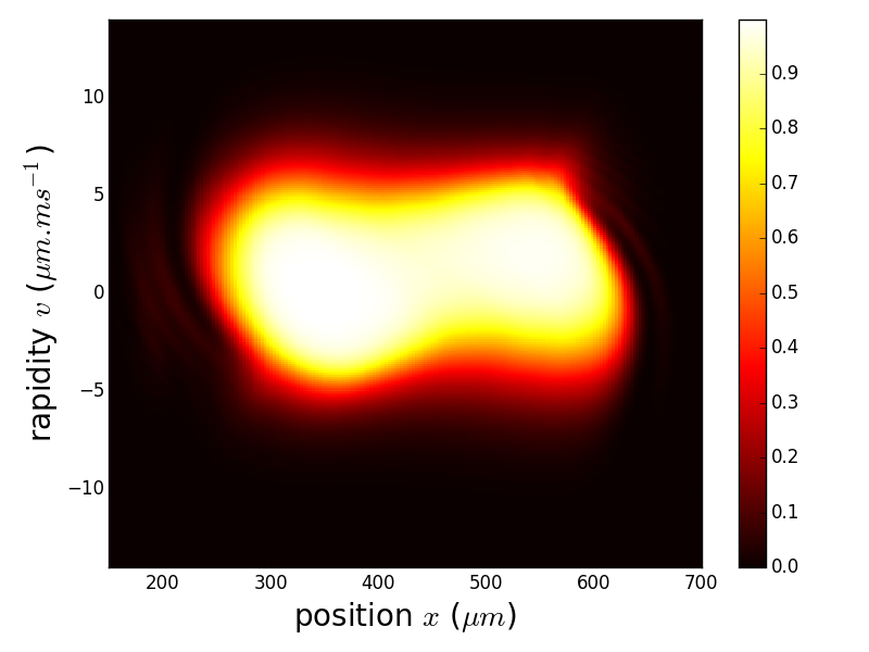
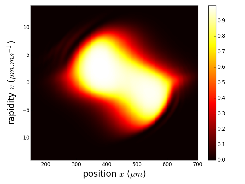
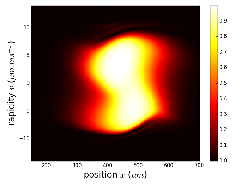
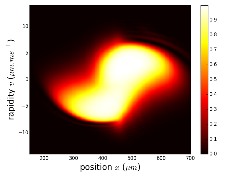
$t=80$ ms	$t=100$ ms	$t=120$ ms	$t=140$ ms
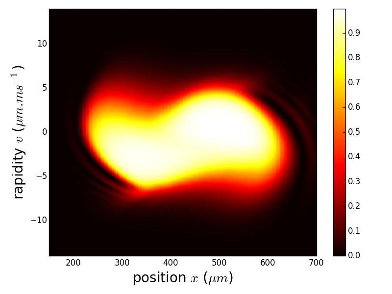
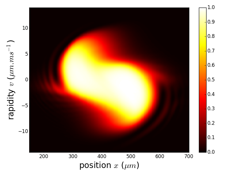
$t=160$ ms	$t=180$ ms

Figure 10: Phase-space occupation $\nu(x,v)$ obtained from GHD for the quench from double-well to harmonic potential shown in Fig. 4 in the main text. The motion is approximately periodic, although one clearly sees that the distribution does not come back exactly to its initial shape after one period; instead, it gets slightly distorted by the interactions between the atoms. The period of the harmonic trap is 154 ms, and we see that the approximate period is roughly 165 ms.