An empirical evaluation of imbalanced data strategies from a practitioner’s point of view

Abstract

This paper evaluates six strategies for mitigating imbalanced data: oversampling, undersampling, ensemble methods, specialized algorithms, class weight adjustments, and a no-mitigation approach referred to as the baseline. These strategies were tested on 58 real-life binary imbalanced datasets with imbalance rates ranging from 3 to 120. We conducted a comparative analysis of 10 under-sampling algorithms, 5 over-sampling algorithms, 2 ensemble methods, and 3 specialized algorithms across eight different performance metrics: accuracy, area under the ROC curve (AUC), balanced accuracy, F1-measure, G-mean, Matthew’s correlation coefficient, precision, and recall. Additionally, we assessed the six strategies on altered datasets, derived from real-life data, with both low (3) and high (100 or 300) imbalance ratios (IR).

The principal finding indicates that the effectiveness of each strategy significantly varies depending on the metric used. The paper also examines a selection of newer algorithms within the categories of specialized algorithms, oversampling, and ensemble methods. The findings suggest that the current hierarchy of best-performing strategies for each metric is unlikely to change with the introduction of newer algorithms.

capbtabboxtable[][]

[a]Artificial Intelligence Lab, REOD.ai, Institute of Computing, University of Campinas, Brazil

1 Introduction

In a class imbalance binary classification problem, the proportion of examples from each class is not equal in the training data and potentially in the test or future data. The minority class is typically referred to as the positive class, while the majority class is the negative class. The imbalance rate (IR) represents the proportion of the majority class relative to the minority class. It is worth noting that sometimes the inverse of this ratio is used as the imbalance ratio. Fortunately, these two distinct uses can be easily identified. Although there is no universally accepted threshold for when the data set is imbalanced, the published research on imbalanced data sets typically focuses on imbalance rates ranging from 3 to 100.

Imbalanced classification problems pose two main challenges. Firstly, detecting the positive class is often more crucial than detecting the negative class. In scenarios like disease detection, misclassifying a person as healthy when they have the disease is more serious than misclassifying a healthy person as having the disease. This is because positive cases require further analysis, unlike false negatives who will not seek treatment since they have been diagnosed as healthy.

Secondly, the scarcity of positive class examples can lead to suboptimal classification results. For instance, when minimizing a global metric, it may be reasonable to prioritize minimizing errors for the majority class while accepting errors for the positive class.

The problem of bias for the negative class can be worsened in local regions, as discussed by Prati et al. (2004), López et al. (2013), and Haixiang et al. (2017). Intrinsic characteristics of the data distribution play a significant role in suboptimal classifiers. These characteristics can be understood by distinguishing safe, borderline, and noisy data (Kubat and Matwin, 1997). Safe data points reside in homogeneous regions of their respective class, while noisy data points are a small set of data points located in regions safe for the other class. Borderline data points are close to the class boundary where some overlap is expected. Classifiers may perform well in defining safe regions, disregard noisy data, but differ in their treatment of borderline regions. Imbalanced problems may result in a conceptual shift from safe regions to borderline regions to noisy regions due to the scarcity or low density of minority class data. This can lead to different classifiers treating them differently, such as treating a borderline region as a safe region for the majority class or considering minority examples in this region as noisy data. Some of the intrinsic characteristics discussed by López et al. (2013) can be understood within this framework of safe, borderline, and noisy data. Small disjuncts (Jo and Japkowicz, 2004) refer to isolated clusters of positive/minority class examples that may be challenging for classifiers to learn. Low density (López et al., 2013) refers to positive examples spread over large volumes, resulting in lower densities and potentially being labeled as noise. Overlapping (Denil and Trappenberg, 2010; Prati et al., 2004) regions have equal numbers of positive and negative examples, leaving the classifier with insufficient information to assign different probabilities to the classes. Noisy data and borderline examples (Napierała et al., 2010) represent instances where safe positive data points may be misinterpreted as noise or exist on the class boundary, posing a higher risk of overlap.

The issue of data set shift represents a more nuanced problem, not directly linked to the safe, borderline, and noisy regions. A fundamental assumption in machine learning is that the test set, on which measurements are performed to make decisions about algorithmic choices, is a valid approximation of future data. However, if there are only a few positive examples, it is improbable that different test sets and future data will be “similar” to each other, particularly concerning the properties of the minority class. Consequently, decisions made by the practitioner based on one test set may not be the most effective when considering the data the system will encounter in the future.

There has been an extensive literature proposing different strategies/techniques/algorithms to deal with imbalanced data. In this paper we will use the term strategy to refer to them all. Most of the strategies discusses in this paper are full fledged algorithms specially the sampling and ensemble strategies, and we will use the term algorithm to discuss particular techniques within these families. But some of the strategies are as simple as doing noting to the data or the classifier (the strategy we call baseline in this paper), while other are to change the base classifier algorithms so that they weight false positive errors more than false negative (a strategy we call class weight). It is a stretch to call these alternatives as algorithms, and thus our use of the term strategy.

For the purposes of his paper, we will classify the different strategies into the following groups or families:

• Baseline This strategy is to apply a “standard”, unmodified classifier to the data. The standard classifier is called a base classifier.

• Cost sensitive: These strategies add a cost to the classification construction algorithm or optimization so that errors for the majority and minority classes have different costs, and thus, the classifier would “try harder” to predict the minority class. A simple solution is to weight the data differently by classes, but the different classifier algorithms must be adapted to take the weight into account. At the time of this writing almost all classifiers in the popular Python package scikit-learn do include a class weight parameter; but gradient boosting machines are one of the important exceptions. A classifier-independent approach is to incorporate the cost into a boosting approach (Domingos, 1999; Sun et al., 2007).

• Sampling approaches. These strategies aim at creating a different training set for the classifier, where the imbalance of the two classes is significantly reduced. The sampling strategies can be further divided into two families.

  • Undersampling approaches reduce the number of majority class elements from the training set. The selection of the data to be removed from the training set can be at random (Drummond et al., 2003) or it can be informed one some measure of how ” important” or “non-important” are the negative data points (Smith et al., 2014) or how “noisy” or “non-noisy” are the negative example data points (Kubat and Matwin, 1997). Lemaître et al. (2017) distinguish between three classes of undersampling:

    • prototype generator where, for example, the negative class is clustered using k-means into $n$ groups, and the centers of the clusters are the new negative data points, and the rest of the negative data is discarted;

    • controlled undesampling techniques, where the final quantity of negative examples can be controlled or set by the user;

    • cleaning undersampling techniques, where only negative data with some “noisy” or “unimportant” characteristic are eliminated from the majority side. An important concept in cleaning undersamplers is a Tomek link - a pair of data from different classes that are each others closest neighbors. One simple cleaning undersampler is the Tomek undersampler (tomekUS) that removes all majority members of Tomek links. Notice that the algorithm is iterative, since removing the majority member of a Tomek link may reveal another Tomek link with the same minority member, but there is no way to control how many majority class data remains after the iterative removal.

  • Oversampling on the other hand, creates new (Chawla et al., 2002; He et al., 2008) or repeat positive examples, increasing their numbers in the training set. As an example of creating new positive examples, the Synthetic Minority Oversampling Technique or SMOTE (Chawla et al., 2002) selects a positive example, and from its $k$ nearest positive neighbours will select a random one. Then it will create a new positive data point in a random position the line segment between these two positives examples.

• Ensemble methods. One can create different under-sampled training sets and train the base classifier on each of these different sets and combine the result of the different classifiers, for example by voting, into a single result. This is a bagging ensemble, based on different under-sampled training set. One can also create a bagging ensemble based on over-sampled training sets. Finally, one can also follow a boosting approach to ensembles, where the training set of each boost is a different under-sampled (or over-sampled) set.

• Specialised classifiers. There has been some research on modifying known algorithms to better deal with imbalanced problems. For example, modifying SVM (Tang et al., 2008), or random forests (Chen et al., 2004), or extreme learning machines (Zong et al., 2013), among others. Also, what in general could be considered an ensemble algorithm for any base classifier, is usually presented or used in the literature with a fixed base classifier, usually a decision tree. In this case we will also treat this as a specialized algorithm. For example EasyEnsemble (Liu et al., 2009) is a bagging of boosted base classifiers, but the literature only considers the case where the base classifier is a decision tree, and thus we will consider it as a specialised classifier and not as a general way of combining any base classifier. Similarly, RUSBoost (Seiffert et al., 2010) could be considered as the general construction procedure of using AdaBoost to construct a boosting ensemble and using random undersampling (thus the “RUS” in the name) on the training set of each boost. But in the literature it is always assumed that the base classifier is a decision tree, and thus we will consider it as a specialised classifier for imbalanced problems.

The families above are not the only way of classifying the strategies into different families, nor it is the case that all strategies fall into the classes above. For example, He and Ma (2013) place the imbalanced data strategies into four main classes: sampling and cost-based (as above) but also kernel-based approaches (Wu and Chang, 2005; Liu and Chen, 2007), which are more specific to SVM classifiers, and one-class approaches (Raskutti and Kowalczyk, 2004) which use one-class classifiers to learn only the minority class. Kernel based approaches will be included into our specialized algorithms class, but one-class approaches (for example, (Raskutti and Kowalczyk, 2004)) are not covered by our taxonomy.

Estabrooks et al. (2004) classify imbalance strategies broadly on internal and external approaches. Internal approaches aim at changing the formulation of a particular classifier so that it can deal better with imbalanced data. Cost-sensitive approaches, such as class weight and kernel-based approaches discussed in the previous paragraph are internal. External approaches assume an unmodified base classifier, and construct a larger classifier by usually combining different instances of the base classifier trained on different samples of the original data. All sampling approaches are external, as is the MetaCost (Domingos, 1999) framework for a cost-sensitive approach, as well as ensemble approaches.

Also, not all strategies proposed in the literature fall within one of our families, as we mentioned above regarding the one-class approaches. Batista et al. (2004) proposed a mixed strategy that combines oversampling followed by a cleaning undersampling, which also is not covered by our taxonomy.

This research attempts to answer the question of what to do with an imbalanced data set from the point of view of a practitioner. We assume that a practitioner:

1. will have time and computer resources to test some but not a very large number of imbalanced strategies, different base classifiers, and different hyperparameters for both the strategies and the base classifiers;

2. prefers using already implemented approaches;

3. may use different metrics;

4. does not have a deep understanding of his or her own data or an understanding of the literature regarding solutions that deal with “similar” data.

We understand a practitioner as someone who is tasked to construct a workable classifier of a particular data set in weeks, as opposed to a researcher that has to construct the best solution for a classification problem in months or years. The practitioner will prefer off-the-shelf classifiers and already implemented imbalance strategies, and will likely not spend the effort to understand his own data in depth beyond the fact that it is imbalanced. The practitioner will not have the time or the tools to understand the intrinsic characteristics of the data set (if there are small disjuncts, overlapping, or low density of the positive class) that may have an impact on the efficiency of different imbalance mitigation strategies.

Let us discuss each of those characteristics of the practitioner, and their impact on the methodological approach taken by this research.

Algorithms in classification are usually dependent on hyperparameters; an algorithm that performs better the other algorithms in a dataset using a particular set of hyperparameter values may perform much worse if the hyperparameters were changed. Thus, almost all practitioners know that one has to perform some hyperparameter search to achieve the best performance of any algorithm. Furthermore, a practitioner also knows that there are very few guarantees that one algorithm will outperform all the others for all data sets. Thus, we assume that a practitioner has both the time and the computational resources to test different algorithms with different hyperparameters for their particular problem.

The same is true for most imbalanced strategies which also have hyperparameters that have to be searched for. But most imbalance strategies have an added degree of freedom: the base classifier itself. Sampling strategies alter the training data that will be fed to a base classifier, and ensemble strategies construct ensembles of a base classifier. Furthermore, the base classifier may have hyperparameters itself. We assume that the practitioner will not only test multiple strategies and their hyperparameters, and different base algorithms and their hyperparameters.

There is a reasonable literature that random forests, gradient boosting machines, and SVM with radial kernels are, in general, the best classifiers for the majority of problems. There is no proof for that, but empirical research on a large set of data sets (Fernández-Delgado et al., 2014; Wainer, 2016) allows one to be reasonably sure that those three classifiers are certainly the first three that should be tested on any problem. We will assume that the practitioner will test these base classifiers. This choice of base classifiers (and how we will analyze their results - see Section 2.4) is an important difference of this research from previous published comparisons (Section 1.1).

The second characteristic is that the practitioner will prefer already implemented and well establish solutions. At the time of the writing of this research, we believe that at least among Python and R implementations of machine learning frameworks, the most well established set of tools to deal with imbalanced are the one provided by the imblearn Python package (Lemaître et al., 2017). Imblearn is compatible with the scikit-learn Python framework for machine learning, and implements a large set of techniques (oversampling, undersampling, some ensemble techniques, and a few specialized algorithms). As a consequence to this research, we tested most of the imbalanced mitigation algorithms implemented in imblearn. The version used in this research is 0.12.0.dev0.

We also assume that the practitioner will not have decision power on the metric used. Metrics are an important issue regarding imbalanced data sets. The main problem with the standard metric, accuracy – the proportion of correct predictions – is that it assigns the same cost for the mis-classifications of both positive and negative examples. As we discussed above, an important aspect of imbalanced problems is that there is some understanding that misclassifying a positive case (a false positive) should be costlier than misclassifying a negative case (a false negative). Different metrics have been proposed to “balance” the mistakes of the classifier on both the positive and negative classes (Japkowicz, 2013).

But we believe that the practitioner will have little control over which metric to use and in this paper we will not advocate one or other metrics as the “correct ones”. We will compare the different strategies using different metrics, in particular the ones listed as the most common ones used in the literature on both techniques and applications of imbalanced problems, according to Haixiang et al. (2017). The metrics are, in order of frequency of use in the literature: AUC, accuracy, gmean, f1, recall, specificity, precision, followed by balanced accuracy and MCC. These metrics are discussed in Section 2.2 and all but specificity are tested in this research. (Specificity is the accuracy of the majority case which we do not believe is an interesting aspect of imbalanced problems.)

Finally, there is a current understanding that the source of difficulties regarding imbalanced datasets is not due to the skewed distribution of the classes but stem from the intrinsic characteristics discussed above (López et al., 2013). If that is true, the best strategy to deal with a particular data set may depend on its particular intrinsic characteristics. We assume that a practitioner will not have the tools or the time to explore these issues regarding their particular data set.

1.1 Related literature

The standard in any research in imbalanced problems, and in machine learning in general, is that researchers that propose new algorithms or methods would compare those algorithms with others across different data sets, using one or sometimes a few metrics. But those comparisons are potentially partial. The choice of the competing algorithms, the choice of data sets used in the comparisons, and the choice of metrics are made by the researchers themselves. This is the standard practice within the research community as a way to provide evidence that one algorithm is a contribution to the research front, and we are not criticising this practice. We will call a comparison as (potentially more) impartial if the author is not the researcher that proposed one of the algorithms that perform well in the comparison. We will discuss some of the relevant impartial comparisons among imbalance mitigation strategies.

Kovács (2019) compares 85 different oversampling algorithms on 104 binary imbalanced data sets, with imbalance rates from 1.8 to 130, with the majority of the data sets having IR below 20. They used gmean, AUC, F1 score, and precision at top 20%, which measures the accuracy on the positive class of the top 20% of the examples with higher internal score (for the classifier). As base classifier they use SVM, decision trees, kNN, and multi-layer perceptrons. When aggregating the results for all data set, for all base classifiers, and for all 4 metrics, the paper recommends polynom-fit-SMOTE (Gazzah and Amara, 2008), ProWSyn (Barua et al., 2013) and SMOTE-IPF (Sáez et al., 2015) as the best oversampling algorithms.

Galar et al. (2012) focus on ensemble-based strategies to deal with imbalanced data. They compare 7 different proposals for cost-based boosting where the weight update rule of AdaBoost is changed to take into consideration the cost of making a minority class error; 4 different algorithms in the family of boosting based ensembles, where sampling strategies of adding or removing data for the training set of each boost is used; 4 different bagging-based ensembles, which use sampling and bagging; and 2 algorithms classified as hybrid. They only use C4.5 as the base classifier and AUC as the quality metric. They conclude that SMOTEBagging, RUSBoost, and UnderBagging are the best strategies in terms of the AUC and RUSBoost seems to be the less computationally complex solution.

López et al. (2013) compare 7 oversampling strategies, 3 cost-sensitive learning, and 5 ensemble-based strategies, using three base classifiers (kNN, C4.5, and SVM) and AUC as the metric. They first compare the strategies within each family and then compare the best in each family to each other. Within the oversampling strategies, they conclude that SMOTE and SMOTE+ENN perform better. For the cost-sensitive approaches, class weight is the winning strategy; and among ensemble-based strategies, RUSBoost, SMOTEBagging, and EasyEnsemble perform better. When comparing the winners among themselves and a no-strategies approach (which we call baseline in this paper), they concluded that, in general, class weight, SMOTE, and SMOTE+ENN perform better than the other strategies (for AUC).

This paper only deals with binary imbalanced problems. There has been recent literature on multiclass imbalanced literature (FernáNdez et al., 2013; Liao, 2008; Wang and Yao, 2012; Abdi and Hashemi, 2015). For these problems, some research follows the path of decomposing the multiclass problem into either OVO or OVA binary imbalanced problems (FernáNdez et al., 2013; Liao, 2008) while other research tackles the full multiclass problem directly (Wang and Yao, 2012; Abdi and Hashemi, 2015).

2 Methods

This section describes the details of the experiment performed in this research. Section 2.1 describes the strategies tested; Section 2.2 discusses the metrics used to evaluate the quality of the classifier and Section 2.3 discusses the datasets used in the evaluation. Section 2.4 discusses the statistical analysis performed in partiuclar the inovative way this research deals with base classifiers; Section 2.5 discusses the different base classifiers and hyperparameters explored in this research; Section 2.6 describes the experimental setup in terms of cross-validation used. Finally and Section 2.7 discusses the public availability of both data and programs to reproduce this research.

2.1 Strategies

The choice of strategies selected for the comparisons was based on one of our assumptions regarding the goals of a practitioner: that she will prefer solutions that are already implemented and established. In this line, we used the python package Imbalanced Learn (Lemaître et al., 2017), and tested some of the strategies implemented therein.

• base Baseline is the null case - the use of a single base classifier with equal weighting for the classes.

• cw The Class Weight strategy weights the positive examples with a higher value so that erring the positive examples is costlier than negative examples. This is an internal strategy and so it depends on changing the base classifier appropriately. Fortunately, standard implementations of random forest, and SVM already accepts a class weight parameter. Unfortunately, at the time of the writing of this report, there is no widely used implementation of gradient boosting classifiers that accept class weight. So this is a low-cost alternative for the practitioner. We fixed the class weight for the negative class as 1 and for the positive as the inverse of the imbalance rate, that is, for an imbalance rate of 100, the positive class has a weight of 100, and the negative weight 1.

• Under the general undersampling approach, we tested the algorithms below. The algorithms names are an abbreviation of the general known name of the algorithm with the US suffix, to indicate that the algorithm belongs to the undersampling family. The algorithms for the other families will also use suffixes: OS for oversampling, SA for specialized algorithms, EN for ensemble algorithms.

  • Controlled undersamplers:

    • randomUS Randomly remove negative examples from the training set. This is the standard controlled undersampling method.

    • nmissUS Near Miss (Mani and Zhang, 2003) (We will not discuss the details of each algorithm.)

  • Cleaning undersamplers

    • tomekUS Tomek undersampler (Tomek, 1976).

    • editUS Edited Nearest Neighbours (Wilson, 1972)

    • allknnUS All K-Nearest Neighbors (Tomek, 1976)

    • condensedUS Condensed Nearest Neighbour (Hart, 1968)

    • onesidedUS One Sided Selection (Kubat et al., 1997)

    • ncleaningUS Neighbourhood Cleaning Rule (Laurikkala, 2001)

    • ihardnessUS Instance Hardness Threshold (Smith et al., 2014)

  • Prototype undersampler:

    • clusterUS Cluster Centroids (Zhang et al., 2010)

• oversampling Under the general oversampling approach we tested the following algorithms:

  • randomOS Random oversampling is the process of randomly selecting with replacement a positive data point, and adding it again to the training set.

  • smoteOS SMOTE or Synthetic Minority Over-sampling Technique (Chawla et al., 2002).

  • adasynOS Adaptive Synthetic (ADASYN) sampling (He et al., 2008)

  • bordersmoteOS Borderline-SMOTE (Han et al., 2005)

  • svmsmoteOS SVM-SMOTE (Nguyen et al., 2011)

• bagging ensemble. We used a two simple strategies based on bagging-based ensemble of the base classifier. The strategies are underbagEN and overbagEN; UnderbagEN is also called underbagging or balanced bagging classifiers, and it uses a standard bagging approach to construct the ensemble, where each bag is balanced using random undersampling. OverbagEN is a standard bagging approach where each bag is balanced using random oversampling.

• specialised classifiers

  • easySA EasyEnsemble (Liu et al., 2009)

  • rusbSA RUSBoost (Seiffert et al., 2010)

  • balrfSA Balanced Random Forests (Chen et al., 2004)

2.2 Metrics

This paper will focus on eight metrics:

• accuracy abbreviated as acc

• area under the ROC curve abbreviated as auc

• balanced accuracy abbreviated as bac

• F1-measure abbreviated as f1

• G-mean (Kubat et al., 1998) abbreviated as gmean

• Matthew’s correlation coefficient(Matthews, 1975) abbreviated as mcc

• precision abbreviated as prec

• recall abbreviated as rec

Let us denote TP as the number of true positives, that is, the correct positive predictions of the classifier; TN as the number of true negatives; FP is the number of false positives, that is data that the classifier predicted as positive which were, in fact, negative; and FN as the number of false negatives. We remind the reader that in this paper and usually in imbalanced problems, the minority class is the positive class and the majority class is the negative class. Then:

acc $$=\frac{TP+TN}{TP+FP+TN+FN}$$

precision $$=\frac{TP}{TP+FP}$$

recall $$=\frac{TP}{TP+FN}$$

specificity $$=\frac{TN}{TN+FP}$$

f1 $$=\frac{2}{\frac{1}{\mbox{precision}}+\frac{1}{\mbox{recall}}}=\frac{2TP}{2TP+FP+FN}$$

bac $$=\frac{\mbox{recall}+\mbox{specificity}}{2}=\frac{\frac{TP}{TP+FN}+\frac{TN}{TN+FP}}{2}$$

gmean $$=\sqrt{\mbox{recall}\times\mbox{specificity}}=\sqrt{\frac{TP}{TP+FN}\times\frac{TN}{TN+FP}}$$

mcc $$=\frac{TP\times TN-FP\times FN}{\sqrt{(TP+FP)(TP+FN)(TN+FP)(TN+FN)}}$$

Accuracy is the proportion of correct predictions. Notice that TP+FN is the total number of positive examples, and thus recall is the accuracy of the positive examples (the proportion of true predictions for the positive examples). Similarly, specificity is the accuracy for the negative cases.

Precision also known as positive predicted value, measures the proportion of data that is indeed positive (TP) among the cases that the classifier determined to be positive (TP+FP); or in other words, how much can one trust the classifier if it outputs a positive classification.

Classifiers usually compute a score value for each data. Let us assume that higher scores are associated with the positive class. Besides computing the score, the classifier also defines a threshold, above which it classifies the example as positive. Changing this threshold, one can change which examples are classified as positive or negative. Lowering the threshold will change the classification of some examples that before were negative to positive. Let assume that some of these were indeed positive (before they were a false negative) but not all of them. Lowering the threshold caused an increase in the true positives and thus an increase in recall. But the newly false positives decrease specificity - the accuracy of negative cases. Therefore, by changing the threshold one can trade recall for specificity, increasing one while decreasing the other. Similarly, one can trade recall for precision by changing the threshold.

The metrics bac, f1 and gmean attempt to balance two of these conflicting/tradeable metrics. bac balances the accuracy of the positive cases (recall) with the accuracy of the negative cases (specificity) by taking the arithmetic mean of both figures. f1 computes the harmonic mean between recall and precision. gmean computes the geometric mean between recall and specificity.

MCC is the Pearson correlation between the predicted and the correct classes. The usual Pearson correlation formula:

$$\rho(X,Y)=\frac{E[XY]-E[X]E[Y]}{\sqrt{E[X^{2}]-E[X]^{2}}\sqrt{E[Y^{2}]-E[Y]^{2}}}$$

where $X$ is the predicted class and $Y$ is the correct class reduces to the mcc formula above when one realizes that:

• $X$ and $Y$ are binary, and thus $E[X^{2}]=E[X]$

• $E[X]$ is the proportion of examples classified as positive ($(TP+FP)/N$), where $N=TP+FP+TN+FN$ is the total number of examples

• $E[Y]$ is the proportion of positive examples ($(TP+FN)/N$),

• $E[XY]$ is the proportion of true positives ($TP/N$)

Area under the curve (AUC) is defined in terms of the receiver operating characteristic (ROC) curve, which is constructed by plotting the recall and specificity (actually 1 - specificity) of the classifier for different values of the score threshold discussed above. The ROC is the convex hull of those points and the AUC is the area of that ROC.

A more intuitive definition is that the AUC is an estimate of the probability that a random positive example will have a higher score than a randomly selected negative example. Under this interpretation, assuming that $f(x)$ is the score for sample $x$, $X_{+}$ is the set of positive examples, and $X_{-}$ the set of negative samples, then

$$auc =\frac{1}{|X_{+}|\times|X_{-}|}\sum_{p\in X_{+},n\in X_{-}}H(f(p)-f(n))$$

where $H(x)=+1$ if $x>0$, and 0 otherwise, is the Heaviside step function. The formula just counts the number of times the score of a positive example is higher than the score of a negative example, divided by the number of pairs.

There are other metrics proposed in the literature (Scott, 2007; Japkowicz, 2013; Branco et al., 2016). In this paper we focus on the eight metrics listed above: auc, acc, f1, gmean, mcc, bac, prec, and rec.

We understand that accuracy is a metric that violates one of the characteristics of an imbalance problem, the intuition that misclassifying positive examples should be more costly that misclassifying negative examples, and thus it is inappropriate as a metric for an imbalanced problem. But given our goal answering the practitioner’s need for practical knowledge on how to solve an imbalanced problem, we cannot disregard that they seem to use accuracy with frequency.

2.3 Data

This paper uses a standard set of data sets that has been used in many imbalanced research. The data that we call natural are a set of 58 real life imbalanced data sets, with imbalance rate ranging from 2.5 to 160. The data is the first three blocks (“Imbalance ratio between 1.5 and 9” and “Imbalance ratio higher than 9” Parts I and II) of the Keel (Alcalá-Fdez et al., 2011) curated data sets on imbalance .

For, the second data, which we call manipulated, we randomly removed either majority or minority data in both the training and test sets so that the resulting data sets would have specific IR of 3, 100, or 300, if possible. The only restriction is that we limit the number of minority data to be at least 8 for the training set and at least 2 for the test set. All 58 datasets could be manipulated to an IR of 3, which represent the low IR examples. Only two of the data sets could be manipulated to an IR of 300, and other 7 could be manipulated for an IR of 100. These 9 data sets represent the examples of high IR.

2.4 Statistical analysis

This paper aims to analyze various strategies within each family of techniques to address imbalanced classification problems. However, the implementation of nearly every strategy necessitates the configuration of hyperparameters. To illustrate, for a controlled undersampling strategy, a decision must be made concerning the final imbalance rate post-undersampling. Besides this hyperparameter, there is a need to select the base classifier (and its hyperparameters) that will process the undersampled training data. Consequently, when comparing different strategies, the choice of base classifier typically must be made, except in the case of specialized algorithms, which are themselves the base algorithm. A pertinent methodological issue is whether the base algorithm is regarded as a nuisance factor, in the broad sense, or as a hyperparameter.

Hyperparameters represent decisions made by the practitioner after testing various alternatives. When executing a comparison of strategies, treating the resulting imbalance ratio (IR) for a controlled undersampler as a hyperparameter implies the assumption that the practitioner, for their specific data set, will conduct a search for possible values for this hyperparameter and select the optimal one. A nuisance factor, on the other hand, is a decision significant for the strategy’s evaluation, but the researcher conducting the comparison does not know which value the practitioner will opt for. Therefore, from the viewpoint of the researcher making the comparison, the solution lies in employing a sufficiently broad range of possible values for the nuisance factor and averaging the results derived from all of them.

Prior research comparing various strategies has often treated the base algorithm as a nuisance factor. This study, however, advocates for treating the base algorithm as a hyperparameter, positing that practitioners will not only explore different values for the strategy’s hyperparameters but will also experiment with different base algorithms and their respective hyperparameters, and choose the best one.

In order to compare strategies, we employ a two-step procedure. Initially, strategies within a single family are compared, with the top-performing strategy designated as the representative for that family. We then carry out a comparison of the representatives across different families. The families of baseline, class weight, and ensemble each comprise a single strategy, so these strategies naturally serve as their respective representatives. However, for the families of undersampling, oversampling, and specialized algorithms, a comparison of all strategies within the family is performed to identify the representative for each metric.

Regarding statistical analysis, we largely adhere to Demsar’s procedure (Demšar, 2006) for comparing multiple classifiers across multiple data sets, albeit with modifications as suggested by Garcia and Herrera (2008) and García et al. (2010). Notably, instead of using the Nemenyi test as advocated by Demsar, we employ a pairwise Wilcoxon test on the ranks of each classifier, with a multi-comparison adjustment of the p-value in accordance with Bergmann and Hommel (Bergmann and Hommel, 1988). For instances where more than nine classifiers were compared, we utilized the Holm procedure (Holm, 1979). The computations were performed using the R package scmamp (Calvo and Santafe, 2016).

Demsar suggested a graphical representation to visualize the resulting comparisons, as depicted in Figure 2. In contrast, we have chosen a more compact representation, utilizing a table to concurrently display the ranking of different strategies and the significance of the differences (Piepho, 2004). Each letter in Table 2 corresponds to a bar in the plot, indicating the lack of statistically significant differences among the algorithms.

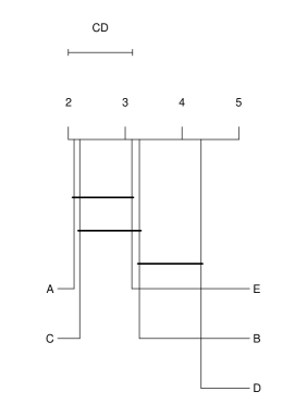
Figure 1: The CD plot of the base results

. algorithm sig A a C ab E ab B  bc D   c

Figure 2: The table representation of the CD plot

Section 2.5 discusses the base classifiers, their hyperparameters, and the hyperparameters for the strategies tested in this research. Once we have a best combination of the base classifier, the base classifier’s hyperparameters, and the strategy’s hyperparameters, we will compare this strategy with the others. Section 2.6 discusses how the data is split into training and test, so the quality of a particular strategy (using a particular metric) is measured in the (multiple) test sets.

2.5 Classifiers and hyperparameters

The base classifiers used are:

• random forest (rf). The hyperparameter range is: number of trees $\in\{100,500,1000\}$.

• SVM with RBF kernel (svm). The hyperparameters are: $C\in\{2^{-5},2^{0},20^{5},20^{10},2^{15}\}$ and $\gamma\in\{2^{-15},2^{-10},2^{-5},2^{0},,2^{5}\}$.

• Gradient boosting machines (gbm). Hyperparameters: learning rate $\in\{0.03,0.1,0.3\}$, max depth $\in\{2,3,5\}$.

The specialised algorithms also have hyperparameters:

• rusbSA: the number of trees is a hyperparameter whose possible values are nboost $\in\{10,20,50,100\}$.

• easySA: The hyperparameter: number of estimators $\in\{3,7,10,20,30\}$

• balrfSA: The hyperparameter: number of trees $\in\{10,50,100,500,1000\}$

The underbagEN and overbagEN in the ensemble family also have a hyperparameter: number of bags $\in\{5,10,20,30\}$.

Finally, some of the over- and undersampling algorithms allow to control for the final imbalance rate after the sampling. For these strategies (randomOS, smoteOS, bordersmoteOS, adasynOS, svmsmoteOS, nmissUS, ihardnessUS, and clusterUS) the final imbalance rate is also a hyperparameter, with the values in $\{0.2,0.4,0.6,0.8,1.0\}$. We did not set the other hyperparameters of the strategies and base classifiers.

2.6 Experimental setup

For each data set, we randomly selected 20% of the data set as the test set. The proportion of classes was the same in both the training and test set but we did not impose any other constraints on the partitioning (against the warnings of (López et al., 2014)).

Let us call solution a combination of a strategy and a base classifier, or the specialised classifiers by themselves. We performed a 3-fold cross-validation on the training set to select the best set of hyperparameters for the solution. For a particular metric, say auc, we tested 10 random samples of the hyperparameters for each solution. The combination of hyperparameters that maximized the mean auc over the three folds was selected. Then the solution was trained on the whole training set, and the auc on the test set was measured. The same process was repeated for the other metrics.

We repeated the process (starting at the random selection of the test set) 3 times, that is, we have three measures of the quality of the solution, which we averaged to have a better estimate. Formally, we used a 3-repetition of a 20% holdout procedure with a nested 3-fold for selecting the hyperparameters.

2.7 Reproducibility

The imbalanced data sets, the programs that run the experiments, the results of all experiments, and the R program to perform the analysis are available at https://figshare.com/s/96b3d7f8d3f74de4b6e3.

3 Results

3.1 Natural data sets

The statistical comparisons between strategies within the OS, US and SA families are displayed in A. The summary of those results are:

For acc:

• undersampling: tomekUS is the algorithm with best mean rank, but it is not significantly different than onesidedUS, ncleaningUS, clusterUS, editnnUS and allknnUS.

• oversampling: best algorithm randomOS but none of the other algorithms are significantly different from it.

• specialised algorithms: rusbSA is the best algorithm, but not significantly better than balrfSA.

• ensemble: overbagEN is significantly better than underbagEN.

For auc:

• undersampling; editUS is the algorithm with the best mean rank, but it is not significantly different than the other undersampling algorithm with the exception of ihardnessUS.

• oversampling: best strategy is svmsmoteOS, but not significantly better than any of the other algorithm.

• specialised algorithms: balrfSA is the best strategy and significantly better than the other two.

• ensemble: overbagEN is not significantly better than underbagEN.

For bac:

• undersampling: randomUS is the best ranked algorithm, but not significantly better than ihardnessUS, clusterUS, and editnnUS.

• oversampling: best algorithm is adasynOS, but not significantly better than any of the others.

• specialised algorithms: balrfSA is the best algorithm, significantly better than any of the others.

• ensemble: underbagEN is significantly better than overbagEN.

For f1:

• undersampling: best strategy: ncleaningUS but not significantly better than the other strategies except ihardnessUS, condensedUS, and nmissUS.

• oversampling: best strategy svmsmoteOS, but not significantly better than any of the other strategies.

• specialised algorithms: balrfSA is the best strategy, significantly better than any of the other strategies.

• ensemble: overbagEN is significantly better than underbagEN.

For gmean:

• undersampling: best algorithm onesidedUS, but not significantly better than tomekUS, ncleaningUS, editnnUS, allknnUS, and condensedUS.

• oversampling: best algorithm svmsmoteOS, but not significantly better any other strategy except bordersmoteOS.

• specialised algorithms: balrfSA is the best algorithm, significantly better than the others.

• ensemble: overbagEN is not significantly better than underbagEN.

For mcc:

• undersampling: best algorithm ihardnessUS but not significantly better than randomUS, clusterUS, allknnUS and editnnUS.

• oversampling: best algorithm adasynOS, but not significantly better than any of the others, except randomOS.

• specialised algorithms: balrfSA is the best algorithm but not significantly better than the otherseasySA‘.

• ensemble: underbagEN is significantly better than overbagEN.

For prec:

• undersampling: best algorithm tomekUS but not significantly better than ncleaningUS, onesidedUS, clusterUS, and allknnUS.

• oversampling: best algorithm randomOS, but not significantly better than the other algorithms except svmsmoteOS.

• specialised algorithms: rusbSA is the best algorithm but not significantly better than balrfSA.

• ensemble: overbagEN is significantly better than underbagEN.

For rec:

• undersampling: best algorithm clusterUS but not significantly better than ihardnessUS, randomUS, condensedUS, and nmissUS.

• oversampling: best algorithm adasynOS, but not significantly better than the other algorithms.

• specialised algorithms: balrfSA is the best algorithm, significantly better than the others.

• ensemble: underbagEN is significantly better than overbagEN

3.1.1 Comparison of the best solutions

We now compare the representative algorithm from each family of oversampling, undersampling, ensemble, and specialized algorithms with the baseline, and class weight, for each metric. The results are displayed in Table 1. Figure 3 report visually the results from Table 1

family	rank	sig	family	rank	sig	family	rank	sig
acc			auc			bac
US	2.81	a	OS	2.79	a	EN	2.42	a
BA	2.87	a	US	3.01	ab	OS	3.16	ab
EN	2.95	a	EN	3.13	ab	US	3.20	ab
OS	3.16	a	CW	3.45	ab	SA	3.57	b
CW	3.33	a	BA	3.89	bc	CW	3.66	b
SA	5.89	b	SA	4.73	c	BA	4.98	c
f1			gmean			mcc
OS	2.75	a	OS	2.60	a	EN	2.19	a
EN	2.76	a	US	3.14	a	US	3.26	b
CW	3.33	ab	EN	3.28	a	SA	3.35	b
US	3.45	ab	BA	3.46	a	OS	3.41	b
BA	3.74	b	CW	3.57	a	CW	3.87	b
SA	4.97	c	SA	4.95	b	BA	4.92	c
prec			rec
US	2.92	a	US	2.35	a
CW	2.93	a	EN	2.89	ab
BA	2.97	a	SA	3.23	b
EN	3.12	a	OS	3.57	b
OS	3.16	a	CW	3.65	b
SA	5.91	b	BA	5.31	c

Table 1: Comparison of the best representatives from each family. rank is the mean rank of the best representative for that family and sig is the indication of statistical non-significance.

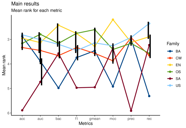
Figure 3: The mean rank of the best representative of each family. Mean rank is better the lower number; vertical dark line indicates that the differences are not statistically significant; horizontal axis indicates the metric.

In summary:

• For acc there is no statistically significant difference among undersampling, baseline, ensemble, oversampling, and cost weights strategies. Specialized algorithms are significantly worse than the best families.

• For auc, there is no statistically significant difference among oversampling, undersampling, ensemble, and cost weight strategies. Specialized algorithms is significantly worse than the other families.

• For bac, ensemble, oversampling and undersampling perform better.

• For f1 oversampling, ensemble, class weight and undesampling perform better.

• For gmean, oversampling, undersampling, ensemble, baseline, and class weight perform better, and specialised algorithms performs significantly worse than the others.

• For mcc ensemble performs significantly better then the alternatives.

• For prec, undersampling, class weight, baseline, ensemble, and oversampling perform better. Specialised algorithms perform significantly worse than the others.

• and finally for rec, undersampling, and ensemble perform better. Baseline performs significantly worse than the others.

3.2 Different imbalance rates

Figure 4 displays the graphic result of the natural data sets and the manipulated data sets for low (3) and high (100 and 300) imbalance rates. For the high IR experiments, because of the smaller number of data sets, the non-significance bars are longer. As expected in most cases the families of strategies maintain their relative positions. But there are some notable changes from low to high IR:

• for acc, it is likely (but not demonstrated by our data) that OS and US will perform better in high IR than the other good strategies (BA, CW and EN).

• for auc, it is likely (but not demonstrated by our data) that OS should perform better for higher IR.

• for gmean, it is likely (but not demonstrated by our data) that OS should perform better for higher IR.

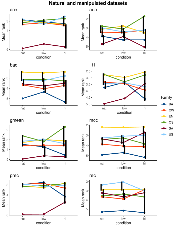
Figure 4: The families of the best strategies for the natural datasets, for the manipulated datasets with low IR (3 and 10) and the manipulated datasets with high IR (100 and 300).

4 Discussion

4.1 Dependency on the quality metric

A critical observation from the results presented above is that the choice of the optimal strategy is profoundly influenced by the metric employed. To our knowledge, this interdependence has not been highlighted in previous literature, and it bears significant implications for both practitioners and researchers. Practitioners must first determine the metric they will employ to assess the quality of the classifier before experimenting with different imbalance strategies. For instance, if the AUC metric is utilized, the baseline or class weight strategies are likely to be the most effective. However, these strategies perform poorly when the MCC metric is applied, with both differences being statistically significant.

As discussed, this research will not provide practitioners with a definitive guide on which metric is most advantageous or which is the “correct” one. We refer the reader to other resources that discuss the various metrics: (Gu et al., 2009), (Jeni et al., 2013), and (Japkowicz, 2013). Readers should also be mindful of works such as (Hernández-Orallo et al., 2012) and (Hand, 2009) that establish a connection between performance metrics and anticipated classification loss when operational conditions (like the ratio of imbalance and the costs of errors for different classes) are unknown in advance.

We believe that the strong dependence of the best strategy on the chosen metric has not been a widely recognized phenomenon in the field. Very few papers, and no comprehensive reviews of the area explicitly state this. Raeder et al. (2012) did briefly observe that certain findings regarding the best classifier for imbalanced problems depend on the evaluation metric, but this observation was used to advocate for the superiority of one metric over others. Zhu et al. (2017) arrived at a conclusion akin to our own but confined their analysis to churn prediction problems. In their study, 24 strategies were tested on 11 churn-specific datasets, leading to the conclusion that “The evaluation metric has a high impact on the (measured, ranked) performance of different techniques.”

The significance of the evaluation metric on the results should inspire future researchers in this field to compare their novel algorithms and strategies using a variety of metrics. A strategy that surpasses alternatives using one metric might also excel with other metrics. By providing comparisons across different metrics, the researcher can deliver valuable insights to practitioners, aiding them in deciding whether to test a specific algorithm or strategy once they have determined the quality metric.

4.2 Base classifier as hyperparameter and relation to previous results

The second important conclusion is that this research seems to contradict the published results, in particular, the results that use AUC as metric (Prati et al., 2015; Galar et al., 2012; López et al., 2013). All of these papers show specialised algorithms (for example RUSBoost) as a winning strategy, while for us, it is the worse family of strategies.

Table 2: Table of comparisons for AUC, when using the hyperparameter method versus when using the nuisance method when dealing with base classifiers.

hyperparameter			nuisance
algorithm	mean.rank	sig	algorithm	mean.rank	sig
OS	2.79	a	OS	2.81	a
US	3.01	ab	SA	3.22	a
EN	3.13	ab	EN	3.26	a
CW	3.45	ab	US	3.59	ab
BA	3.89	bc	CW	3.66	ab
SA	4.73	c	BA	4.47	b

A significant distinction between our study and previous research lies in the treatment of the base algorithm as a hyperparameter in our analysis (as detailed in Section 2.4), while other studies regard it as a nuisance factor. Besides this analytical difference, past literature also often employs weak classifiers, or base classifiers that are likely suboptimal for the data. Naturally, in a nuisance factor analysis, where the average over possible values of the base classifier is calculated, it would be reasonable to include simpler algorithms in the average. Studies by Prati et al. (2015) and López et al. (2013) include SVMs alongside less powerful classifiers such as decision tree, rule induction, and naive Bayes, all with fixed hyperparameters. In contrast, our research not only treats the base algorithm as a hyperparameter (and seeks better hyperparameters for the base classifiers themselves) but also uses “stronger” base classifiers, or those more likely to perform well on the data.

To illustrate the impact of our approach, Table 2 presents a comparison of the statistical tests of AUC for our methodology, and the results from including weaker base classifiers into the alternatives (in this case, 1-NN and CART decision trees) and averaging the results for all base classifiers, that is treating base classifiers as a nuisance factor.

The revised results partially align with the conclusions of prior research. For instance, Galar et al. (2012), who employed only decision trees as base classifiers, identified RUSBoost (SA) and Underbagging (EN) as winning strategies, both of which rank as the top two strategies in Table 2 without any statistically significant differences. These results, however, show less congruence with López et al. (2013), who found SMOTE (OS), RUSBoost (SA), and class weight (CW) as winning strategies, obtained using k-NN, C4.5, and SVM (all with fixed hyperparameters) as base classifiers.

Specialized algorithms, since they do not have base classifiers, benefit a lot from the nuisance methodology. Strategies on the other families will be weighted down by averaging their results using less powerful base classifiers while specialized algorithms will not.

4.3 Testing newer algorithms

A potential critique of this research is its reliance on the particular strategies and algorithms tested, which may not represent the cutting edge within each family. This section demonstrates that our main findings remain relatively stable when we introduce newer algorithms. Initially, we augmented our analysis by including only newer algorithms from each family, followed by an inclusive approach where we incorporated all new algorithms across families.

Within the OS family, we based our selection of newer (or more modern) algorithms on an analysis by Kovács (2019), which compared 85 oversampling algorithms across three metrics: AUC, F1, and gmean. We chose the top three algorithms for each metric. The new OS algorithms tested included: polynom-fit-SMOTE (Gazzah and Amara, 2008), ProWSyn (Barua et al., 2013), SMOTE-IPF (Sáez et al., 2015), Lee (Lee et al., 2015), G-SMOTE (Sandhan and Choi, 2014), LVQ-SMOTE (Nakamura et al., 2013), Assembled-SMOTE (Zhou et al., 2013), and SMOBD (Wang et al., 2012). We extend our thanks to the authors for their contributions to the implementation of these and other oversampling algorithms.

For the ensemble family, our analysis so far considered two basic algorithms: underbagging and overbagging. To examine new ensemble strategies, we leveraged the implementation of various ensemble alternatives by Liu et al. (2021). Among these, we tested the overboost ensemble, which is a boosting approach that incorporates oversampling in its boosting stages, and the self-paced ensemble (Liu et al., 2020), a novel proposal for addressing imbalanced datasets.

In the specialized algorithm category, we included the AdaCC (Iosifidis et al., 2023) algorithm in our tests.

Our experimental process involved the sequential addition of new strategies from one family at a time and then the simultaneous addition of all the new strategies. Figure 5 compares the original ranking of the families with the updated rankings after incorporating the new strategies, culminating in the final entry where all new strategies are included.

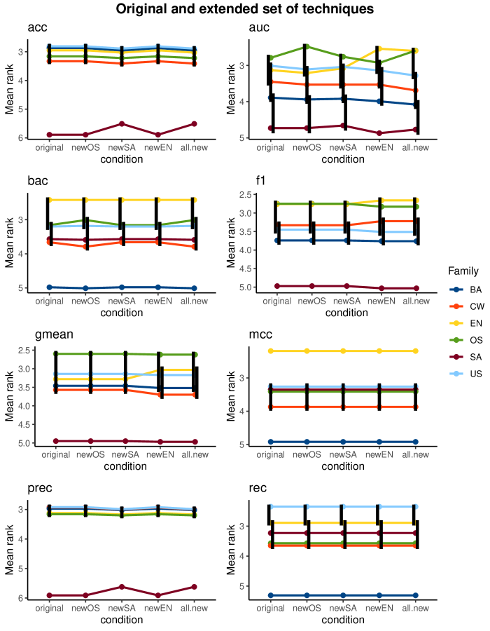
Figure 5: The comparison of our original results and results by adding newer algorithms in the OS, EN and SA families. newOS are the result of adding only newer OS strategies, and similarly for newEN and newSA. .

The integration of more sophisticated (or at least more contemporary) oversampling (OS) algorithms does not alter the relative ranking of the best-performing algorithms for each metric, with the exception of the area under the curve (AUC) and balanced accuracy (BAC). For AUC, OS is already the leading family of strategies (though not significantly superior to some others); however, the introduction of newer algorithms appears to further distinguish OS from the rest (yet without a significant difference from ensemble (EN) and undersampling (US)). Consequently, in the case of AUC, newer OS algorithms are likely to result in performance improvements. Likewise, newer EN algorithms also enhance that family’s average ranking. For BAC, the latest OS algorithms have shifted OS from the third to the second-best strategy family (although not significantly different from the other two).

The introduction of more sophisticated EN algorithms seems to have a greater impact on the EN family’s relative ranking, especially for AUC but also for the F1-score and geometric mean (gmean). Conversely, the specialized algorithms (SA) are consistently outperformed by the other families, and the addition of new SA algorithms does little to change this.

Therefore, for all metrics, with the potential exception of AUC, one can reasonably project the findings of this study to newer or forthcoming algorithms—if this paper concludes that for Matthews correlation coefficient (MCC), ensemble strategies are likely the best option based on the tested strategies, it is safe to assume that a newly published OS algorithm would not overturn that conclusion. More definitively, a practitioner using MCC as their metric should focus on testing some of the EN strategies discussed in this paper, and probably avoid expending resources on implementing or testing a newly published OS algorithm.

AUC, however, appears to be a metric that is more susceptible to fluctuations with the introduction of newer algorithms. In our experiments, newer algorithms in the OS family did improve its relative ranking, a trend that was also observed with the introduction of newer EN algorithms. This indicates that some of these newer algorithms did outperform their older counterparts. Therefore, a practitioner using AUC as a metric should stay informed about newer algorithms, especially among the families that generally perform well for this metric: OS, EN, and US (for which we did not test newer algorithms).

5 Conclusions

5.1 How a practitioner should use these results

Once the practitioner selects a quality metric, they should refer to Figure 3 or Table 1 to identify the which strategies are most effective according to that metric. Additionally, practitioners must consider the data’s imbalance rate (IR), especially in cases of high IR. For these instances, the practitioner should review the trends for high IR depicted in Figure LABEL:fig:high_ir. It is important to note that these trends may not be definitive due to the limited size of the datasets, which prevents achieving statistical significance. Nonetheless, for those using metrics such as AUC or G-mean, oversampling is highly recommended.

Upon determining the suitable strategy families, practitioners should refer to section 3.1 or Appendix A, which details the top-performing algorithms within these families. Practitioners are encouraged to test all, or at the very least, the majority of the top-ranked algorithms from the chosen families.

Finally, practitioners should not overlook the importance of selecting different base classifiers for strategies that require them and should invest effort into hyperparameter tuning for both the algorithm and the base classifiers. Section 2.5 provides a list of hyperparameters and the values that have been utilized in this study.

5.2 How a researcher should use these results

This paper offers two key recommendations for researchers who are developing new algorithms to address imbalanced problems. The first, and in the authors’ view, the most pressing research direction, concerns the alignment of strategies with various metrics. A pertinent question arises: why do ensemble algorithms excel with the MCC metric, while specialized algorithms perform poorly with the precision metric? A deeper exploration into how these strategies correlate with specific metrics could illuminate potential enhancements within those algorithmic families. For instance, a better grasp of why the MCC metric aligns so well with ensemble strategies might lead to advancements in ensemble algorithms.

Secondly, researchers developing a new algorithm within a given family should benchmark it against other algorithms in the same family, particularly for the metrics where that family excels. If practitioners are to adopt the new algorithm, it stands a better chance if it is among the top performers for the metric of interest, rather than simply being the best within its family.

Appendix A Results on the natural data sets: each family

algorithm	rank	sig	algorithm	rank	sig	algorithm	rank	sig
acc			auc			bac
tomekUS	4.04	a	editnnUS	4.53	a	randomUS	3.53	a
onesidedUS	4.33	a	allknnUS	4.84	a	ihardnessUS	4.03	ab
ncleaningUS	4.66	ab	ncleaningUS	4.94	a	clusterUS	4.72	abc
clusterUS	4.95	ab	onesidedUS	5.01	a	editnnUS	5.19	abcd
editnnUS	5.11	ab	tomekUS	5.09	a	allknnUS	5.47	bcd
allknnUS	5.50	ab	randomUS	5.65	ab	ncleaningUS	5.66	bcd
nmissUS	6.13	bc	clusterUS	5.90	ab	condensedUS	6.23	cd
randomUS	6.20	bc	condensedUS	5.99	ab	nmissUS	6.48	cd
condensedUS	6.25	bc	nmissUS	6.14	ab	tomekUS	6.72	d
ihardnessUS	7.84	c	ihardnessUS	6.93	b	onesidedUS	6.96	d
f1			gmean			mcc
ncleaningUS	4.35	a	onesidedUS	4.11	a	ihardnessUS	3.79	a
tomekUS	4.35	a	tomekUS	4.29	a	randomUS	4.05	ab
onesidedUS	4.52	a	ncleaningUS	4.36	a	clusterUS	4.73	abc
editnnUS	4.84	a	editnnUS	4.42	a	allknnUS	5.20	abcd
allknnUS	5.22	ab	allknnUS	4.47	a	editnnUS	5.31	abcd
clusterUS	5.34	ab	condensedUS	5.72	ab	ncleaningUS	5.70	bcde
randomUS	5.66	abc	randomUS	6.22	bc	nmissUS	6.10	cde
ihardnessUS	6.63	bc	clusterUS	6.23	bc	condensedUS	6.15	cde
condensedUS	6.67	bc	ihardnessUS	7.33	bc	tomekUS	6.78	de
nmissUS	7.42	c	nmissUS	7.84	c	onesidedUS	7.19	e
prec			rec
tomekUS	3.58	a	clusterUS	3.48	a
ncleaningUS	3.94	ab	ihardnessUS	3.52	a
onesidedUS	4.23	ab	randomUS	3.68	a
clusterUS	5.04	abc	condensedUS	4.27	ab
allknnUS	5.32	abc	nmissUS	4.45	ab
editnnUS	5.44	bc	allknnUS	5.72	bc
randomUS	5.68	bcd	editnnUS	6.20	c
nmissUS	6.49	cde	ncleaningUS	7.24	cd
condensedUS	7.33	de	onesidedUS	8.18	d
ihardnessUS	7.95	e	tomekUS	8.26	d

Table 3: Undersampling algorithms: results of the statistical test.

algorithm	rank	sig	algorithm	rank	sig	algorithm	rank	sig
acc			auc			bac
randomOS	2.84	a	svmsmoteOS	2.84	a	adasynOS	2.53	a
smoteOS	2.95	a	smoteOS	2.85	a	smoteOS	2.96	a
svmsmoteOS	2.99	a	adasynOS	2.95	a	svmsmoteOS	3.03	a
adasynOS	3.04	a	randomOS	3.15	a	bordersmoteOS	3.14	a
bordersmoteOS	3.17	a	bordersmoteOS	3.22	a	randomOS	3.34	a
f1			gmean			mcc
svmsmoteOS	2.74	a	svmsmoteOS	2.55	a	adasynOS	2.44	a
randomOS	2.91	a	smoteOS	2.70	a	smoteOS	2.99	ab
adasynOS	3.07	a	adasynOS	2.98	ab	bordersmoteOS	3.07	ab
bordersmoteOS	3.13	a	randomOS	3.16	ab	svmsmoteOS	3.09	ab
smoteOS	3.15	a	bordersmoteOS	3.61	b	randomOS	3.41	b
prec			rec
randomOS	2.25	a	adasynOS	2.56	a
svmsmoteOS	2.97	ab	smoteOS	2.97	a
smoteOS	3.00	b	bordersmoteOS	2.98	a
bordersmoteOS	3.23	b	randomOS	3.13	a
adasynOS	3.55	b	svmsmoteOS	3.36	a

Table 4: Oversampling algorithms: results of the statistical test.

algorithm	rank	sig	algorithm	rank	sig	algorithm	rank	sig
acc			auc			bac
rusbSA	1.78	a	balrfSA	1.50	a	balrfSA	1.46	a
balrfSA	1.90	a	easySA	2.20	b	easySA	1.96	b
easySA	2.33	b	rusbSA	2.30	b	rusbSA	2.59	c
f1			gmean			mcc
balrfSA	1.43	a	balrfSA	1.52	a	balrfSA	1.59	a
easySA	2.09	b	easySA	2.16	b	easySA	1.94	a
rusbSA	2.47	c	rusbSA	2.32	b	rusbSA	2.47	b
prec			rec
balrfSA	1.76	a	balrfSA	1.49	a
rusbSA	1.89	a	easySA	1.89	b
easySA	2.35	b	rusbSA	2.62	c

Table 5: Specialized algorithms: results of the statistical test.

algorithm	rank	sig	algorithm	rank	sig	algorithm	rank	sig
acc			auc			bac
overbagEN	1.17	a	overbagEN	1.46	a	underbagEN	1.29	a
underbagEN	1.83	b	underbagEN	1.54	a	overbagEN	1.71	b
f1			gmean			mcc
overbagEN	1.28	a	overbagEN	1.41	a	underbagEN	1.24	a
underbagEN	1.72	b	underbagEN	1.59	a	overbagEN	1.76	b
prec			rec
overbagEN	1.12	a	underbagEN	1.41	a
underbagEN	1.88	b	overbagEN	1.59	b

Table 6: Ensemble strategies: results of the statistical test

Appendix B Results on new algorithms

original

newOS

newSA

newEN

all new

algorithm

rank

sig

algorithm

rank

sig

algorithm

rank

sig

algorithm

rank

sig

algorithm

rank

sig

acc

US

2.81

a

US

2.81

a

US

2.89

a

US

2.81

a

US

2.89

a

BA

2.87

a

BA

2.87

a

BA

2.96

a

BA

2.87

a

BA

2.96

a

EN

2.95

a

EN

2.95

a

EN

3.03

a

EN

2.95

a

EN

3.03

a

OS

3.16

a

OS

3.16

a

OS

3.22

a

OS

3.16

a

OS

3.22

a

CW

3.33

a

CW

3.33

a

CW

3.41

a

CW

3.33

a

CW

3.41

a

SA

5.89

b

SA

5.89

b

SA

5.51

b

SA

5.89

b

SA

5.51

b

auc

OS

2.79

a

OS

2.48

a

OS

2.76

a

EN

2.54

a

OS

2.59

a

US

3.01

ab

US

3.11

ab

US

3.04

ab

OS

2.93

ab

EN

2.60

a

EN

3.13

ab

EN

3.21

ab

EN

3.08

ab

US

3.14

abc

US

3.28

ab

CW

3.45

ab

CW

3.53

b

CW

3.53

ab

CW

3.53

bc

CW

3.69

b

BA

3.89

bc

BA

3.94

bc

BA

3.92

bc

BA

3.99

c

BA

4.08

bc

SA

4.73

c

SA

4.73

c

SA

4.66

c

SA

4.87

d

SA

4.77

c

bac

EN

2.42

a

EN

2.42

a

EN

2.42

a

EN

2.42

a

EN

2.42

a

OS

3.16

ab

OS

3.01

ab

OS

3.16

ab

OS

3.16

ab

OS

3.01

ab

US

3.20

ab

US

3.18

ab

US

3.20

ab

US

3.20

ab

US

3.18

ab

SA

3.57

b

SA

3.59

b

SA

3.57

b

SA

3.57

b

SA

3.59

b

CW

3.66

b

CW

3.79

b

CW

3.66

b

CW

3.66

b

CW

3.79

b

BA

4.98

c

BA

5.01

c

BA

4.98

c

BA

4.98

c

BA

5.01

c

f1

OS

2.75

a

OS

2.75

a

OS

2.75

a

EN

2.66

a

EN

2.66

a

EN

2.76

a

EN

2.76

a

EN

2.76

a

OS

2.83

a

OS

2.83

a

CW

3.33

ab

CW

3.33

ab

CW

3.33

ab

CW

3.22

ab

CW

3.22

ab

US

3.45

ab

US

3.45

ab

US

3.45

ab

US

3.51

ab

US

3.51

ab

BA

3.74

b

BA

3.74

b

BA

3.74

b

BA

3.76

b

BA

3.76

b

SA

4.97

c

SA

4.97

c

SA

4.97

c

SA

5.03

c

SA

5.03

c

gmean

OS

2.60

a

OS

2.60

a

OS

2.60

a

OS

2.62

a

OS

2.62

a

US

3.14

a

US

3.14

a

US

3.14

a

EN

3.03

ab

EN

3.03

ab

EN

3.28

a

EN

3.28

a

EN

3.28

a

US

3.17

ab

US

3.17

ab

BA

3.46

a

BA

3.46

a

BA

3.46

a

BA

3.52

ab

BA

3.52

ab

CW

3.57

a

CW

3.57

a

CW

3.57

a

CW

3.70

b

CW

3.70

b

SA

4.95

b

SA

4.95

b

SA

4.95

b

SA

4.97

c

SA

4.97

c

mcc

EN

2.19

a

EN

2.19

a

EN

2.19

a

EN

2.19

a

EN

2.19

a

US

3.26

b

US

3.26

b

US

3.26

b

US

3.26

b

US

3.26

b

SA

3.35

b

SA

3.35

b

SA

3.35

b

SA

3.35

b

SA

3.35

b

OS

3.41

b

OS

3.41

b

OS

3.41

b

OS

3.41

b

OS

3.41

b

CW

3.87

b

CW

3.87

b

CW

3.87

b

CW

3.87

b

CW

3.87

b

BA

4.92

c

BA

4.92

c

BA

4.92

c

BA

4.92

c

BA

4.92

c

prec

US

2.92

a

US

2.92

a

US

2.99

a

US

2.92

a

US

2.99

a

CW

2.93

a

CW

2.93

a

CW

3.00

a

CW

2.93

a

CW

3.00

a

BA

2.97

a

BA

2.97

a

BA

3.02

a

BA

2.97

a

BA

3.02

a

EN

3.12

a

EN

3.12

a

EN

3.17

a

EN

3.12

a

EN

3.17

a

OS

3.16

a

OS

3.16

a

OS

3.20

a

OS

3.16

a

OS

3.20

a

SA

5.91

b

SA

5.91

b

SA

5.62

b

SA

5.91

b

SA

5.62

b

rec

US

2.35

a

US

2.35

a

US

2.35

a

US

2.35

a

US

2.35

a

EN

2.89

ab

EN

2.89

ab

EN

2.89

ab

EN

2.89

ab

EN

2.89

ab

SA

3.23

b

SA

3.23

b

SA

3.23

b

SA

3.23

b

SA

3.23

b

OS

3.57

b

OS

3.57

b

OS

3.57

b

OS

3.57

b

OS

3.57

b

CW

3.65

b

CW

3.65

b

CW

3.65

b

CW

3.65

b

CW

3.65

b

BA

5.31

c

BA

5.31

c

BA

5.31

c

BA

5.31

c

BA

5.31

c

Table 7: Introduction of more modern strategies: results of the statistical tests.

References

- Abdi and Hashemi (2015) Lida Abdi and Sattar Hashemi. To combat multi-class imbalanced problems by means of over-sampling techniques. IEEE Transactions on Knowledge & Data Engineering, 28(1):238–251, 2015.
- Alcalá-Fdez et al. (2011) Jesús Alcalá-Fdez, Alberto Fernández, Julián Luengo, Joaquín Derrac, Salvador García, Luciano Sánchez, and Francisco Herrera. Keel data-mining software tool: data set repository, integration of algorithms and experimental analysis framework. Journal of Multiple-Valued Logic & Soft Computing, 17, 2011.
- Barua et al. (2013) Sukarna Barua, Md Monirul Islam, and Kazuyuki Murase. Prowsyn: Proximity weighted synthetic oversampling technique for imbalanced data set learning. In Pacific-Asia Conference on Knowledge Discovery and Data Mining, pages 317–328. Springer, 2013.
- Batista et al. (2004) Gustavo EAPA Batista, Ronaldo C Prati, and Maria Carolina Monard. A study of the behavior of several methods for balancing machine learning training data. ACM SIGKDD explorations newsletter, 6(1):20–29, 2004.
- Bergmann and Hommel (1988) Beate Bergmann and Gerhard Hommel. Improvements of general multiple test procedures for redundant systems of hypotheses. In Multiple Hypotheses Testing, pages 100–115. Springer, 1988.
- Branco et al. (2016) Paula Branco, Luís Torgo, and Rita P Ribeiro. A survey of predictive modeling on imbalanced domains. ACM Computing Surveys (CSUR), 49(2):31, 2016.
- Calvo and Santafe (2016) Borja Calvo and Guzman Santafe. scmamp: Statistical comparison of multiple algorithms in multiple problems. The R Journal, 8(1), 2016.
- Chawla et al. (2002) Nitesh V Chawla, Kevin W Bowyer, Lawrence O Hall, and W Philip Kegelmeyer. Smote: synthetic minority over-sampling technique. Journal of artificial intelligence research, 16:321–357, 2002.
- Chen et al. (2004) Chao Chen, A Liaw, and L Breiman. Using random forest to learn imbalanced data. 2004. University of California, Berkeley, 2004.
- Demšar (2006) Janez Demšar. Statistical comparisons of classifiers over multiple data sets. Journal of Machine learning research, 7(Jan):1–30, 2006.
- Denil and Trappenberg (2010) Misha Denil and Thomas Trappenberg. Overlap versus imbalance. In Canadian Conference on Artificial Intelligence, pages 220–231. Springer, 2010.
- Domingos (1999) Pedro Domingos. Metacost: A general method for making classifiers cost-sensitive. In Proceedings ACM SIGKDD international conference on Knowledge discovery and data mining, pages 155–164. ACM, 1999.
- Drummond et al. (2003) Chris Drummond, Robert C Holte, et al. C4.5, class imbalance, and cost sensitivity: why under-sampling beats over-sampling. In Workshop on learning from imbalanced datasets II, volume 11, pages 1–8. Citeseer, 2003.
- Estabrooks et al. (2004) Andrew Estabrooks, Taeho Jo, and Nathalie Japkowicz. A multiple resampling method for learning from imbalanced data sets. Computational intelligence, 20(1):18–36, 2004.
- FernáNdez et al. (2013) Alberto FernáNdez, Victoria LóPez, Mikel Galar, MaríA José Del Jesus, and Francisco Herrera. Analysing the classification of imbalanced data-sets with multiple classes: Binarization techniques and ad-hoc approaches. Knowledge-based systems, 42:97–110, 2013.
- Fernández-Delgado et al. (2014) Manuel Fernández-Delgado, Eva Cernadas, Senén Barro, and Dinani Amorim. Do we need hundreds of classifiers to solve real world classification problems. Journal Machine Learning Reseach, 15(1):3133–3181, 2014.
- Galar et al. (2012) Mikel Galar, Alberto Fernandez, Edurne Barrenechea, Humberto Bustince, and Francisco Herrera. A review on ensembles for the class imbalance problem: bagging-, boosting-, and hybrid-based approaches. IEEE Transactions on Systems, Man, and Cybernetics, Part C (Applications and Reviews), 42(4):463–484, 2012.
- Garcia and Herrera (2008) Salvador Garcia and Francisco Herrera. An extension on“statistical comparisons of classifiers over multiple data sets”for all pairwise comparisons. Journal of Machine Learning Research, 9(Dec):2677–2694, 2008.
- García et al. (2010) Salvador García, Alberto Fernández, Julián Luengo, and Francisco Herrera. Advanced nonparametric tests for multiple comparisons in the design of experiments in computational intelligence and data mining: Experimental analysis of power. Information Sciences, 180(10):2044–2064, 2010.
- Gazzah and Amara (2008) Sami Gazzah and Najoua Essoukri Ben Amara. New oversampling approaches based on polynomial fitting for imbalanced data sets. In 2008 The Eighth IAPR International Workshop on Document Analysis Systems, pages 677–684. IEEE, 2008.
- Gu et al. (2009) Qiong Gu, Li Zhu, and Zhihua Cai. Evaluation measures of the classification performance of imbalanced data sets. In International Symposium on Intelligence Computation and Applications, pages 461–471. Springer, 2009.
- Haixiang et al. (2017) Guo Haixiang, Li Yijing, Jennifer Shang, Gu Mingyun, Huang Yuanyue, and Gong Bing. Learning from class-imbalanced data: Review of methods and applications. Expert Systems with Applications, 73:220–239, 2017.
- Han et al. (2005) Hui Han, Wen-Yuan Wang, and Bing-Huan Mao. Borderline-smote: a new over-sampling method in imbalanced data sets learning. In International Conference on Intelligent Computing, pages 878–887. Springer, 2005.
- Hand (2009) David J Hand. Measuring classifier performance: a coherent alternative to the area under the roc curve. Machine learning, 77(1):103–123, 2009.
- Hart (1968) Peter Hart. The condensed nearest neighbor rule (corresp.). IEEE transactions on information theory, 14(3):515–516, 1968.
- He and Ma (2013) Haibo He and Yunqian Ma, editors. Imbalanced learning: foundations, algorithms, and applications. John Wiley & Sons, 2013.
- He et al. (2008) Haibo He, Yang Bai, Edwardo A Garcia, and Shutao Li. Adasyn: Adaptive synthetic sampling approach for imbalanced learning. In Neural Networks, 2008. IJCNN 2008.(IEEE World Congress on Computational Intelligence). IEEE International Joint Conference on, pages 1322–1328. IEEE, 2008.
- Hernández-Orallo et al. (2012) José Hernández-Orallo, Peter Flach, and Cèsar Ferri. A unified view of performance metrics: translating threshold choice into expected classification loss. Journal of Machine Learning Research, 13(Oct):2813–2869, 2012.
- Holm (1979) Sture Holm. A simple sequentially rejective multiple test procedure. Scandinavian journal of statistics, pages 65–70, 1979.
- Iosifidis et al. (2023) Vasileios Iosifidis, Symeon Papadopoulos, Bodo Rosenhahn, and Eirini Ntoutsi. Adacc: cumulative cost-sensitive boosting for imbalanced classification. Knowledge and Information Systems, 65(2):789–826, 2023.
- Japkowicz (2013) Nathalie Japkowicz. Imbalanced learning: foundations, algorithms, and applications, chapter Assessment metrics for imbalanced learning, pages 187–206. In He and Ma (2013), 2013.
- Jeni et al. (2013) László A Jeni, Jeffrey F Cohn, and Fernando De La Torre. Facing imbalanced data–recommendations for the use of performance metrics. In Affective Computing and Intelligent Interaction (ACII), 2013 Humaine Association Conference on, pages 245–251. IEEE, 2013.
- Jo and Japkowicz (2004) Taeho Jo and Nathalie Japkowicz. Class imbalances versus small disjuncts. ACM Sigkdd Explorations Newsletter, 6(1):40–49, 2004.
- Kovács (2019) György Kovács. An empirical comparison and evaluation of minority oversampling techniques on a large number of imbalanced datasets. Applied Soft Computing, 83:105662, 2019. doi: 10.1016/j.asoc.2019.105662. (IF-2019=4.873).
- Kubat and Matwin (1997) Miroslav Kubat and Stan Matwin. Addressing the curse of imbalanced training sets: one-sided selection. In ICML, pages 179–186, 1997.
- Kubat et al. (1997) Miroslav Kubat, Stan Matwin, et al. Addressing the curse of imbalanced training sets: one-sided selection. In ICML, page 179. Citeseer, 1997.
- Kubat et al. (1998) Miroslav Kubat, Robert C Holte, and Stan Matwin. Machine learning for the detection of oil spills in satellite radar images. Machine learning, 30(2-3):195–215, 1998.
- Laurikkala (2001) Jorma Laurikkala. Improving identification of difficult small classes by balancing class distribution. In Conference on artificial intelligence in medicine in Europe, pages 63–66. Springer, 2001.
- Lee et al. (2015) Jaedong Lee, Noo-ri Kim, and Jee-Hyong Lee. An over-sampling technique with rejection for imbalanced class learning. In Proceedings of the 9th International Conference on Ubiquitous Information Management and Communication, pages 1–6, 2015.
- Lemaître et al. (2017) Guillaume Lemaître, Fernando Nogueira, and Christos K. Aridas. Imbalanced-learn: A python toolbox to tackle the curse of imbalanced datasets in machine learning. Journal of Machine Learning Research, 18(17):1–5, 2017.
- Liao (2008) T Warren Liao. Classification of weld flaws with imbalanced class data. Expert Systems with Applications, 35(3):1041–1052, 2008.
- Liu et al. (2009) Xu-Ying Liu, Jianxin Wu, and Zhi-Hua Zhou. Exploratory undersampling for class-imbalance learning. IEEE Transactions on Systems, Man, and Cybernetics, Part B (Cybernetics), 39(2):539–550, 2009.
- Liu and Chen (2007) Yi-Hung Liu and Yen-Ting Chen. Face recognition using total margin-based adaptive fuzzy support vector machines. IEEE Transactions on Neural Networks, 18(1):178–192, 2007.
- Liu et al. (2020) Zhining Liu, Wei Cao, Zhifeng Gao, Jiang Bian, Hechang Chen, Yi Chang, and Tie-Yan Liu. Self-paced ensemble for highly imbalanced massive data classification. In 2020 IEEE 36th international conference on data engineering (ICDE), pages 841–852. IEEE, 2020.
- Liu et al. (2021) Zhining Liu, Jian Kang, Hanghang Tong, and Yi Chang. Imbens: ensemble class-imbalanced learning in python. arXiv preprint arXiv:2111.12776, 2021.
- López et al. (2013) Victoria López, Alberto Fernández, Salvador García, Vasile Palade, and Francisco Herrera. An insight into classification with imbalanced data: Empirical results and current trends on using data intrinsic characteristics. Information Sciences, 250:113–141, 2013.
- López et al. (2014) Victoria López, Alberto Fernández, and Francisco Herrera. On the importance of the validation technique for classification with imbalanced datasets: Addressing covariate shift when data is skewed. Information Sciences, 257:1–13, 2014.
- Mani and Zhang (2003) Inderjeet Mani and I Zhang. knn approach to unbalanced data distributions: a case study involving information extraction. In Proceedings of workshop on learning from imbalanced datasets, volume 126, pages 1–7. ICML, 2003.
- Matthews (1975) Brian W Matthews. Comparison of the predicted and observed secondary structure of t4 phage lysozyme. Biochimica et Biophysica Acta (BBA)-Protein Structure, 405(2):442–451, 1975.
- Nakamura et al. (2013) Munehiro Nakamura, Yusuke Kajiwara, Atsushi Otsuka, and Haruhiko Kimura. LVQ-SMOTE–learning vector quantization based synthetic minority over–sampling technique for biomedical data. BioData mining, 6(1):1–10, 2013.
- Napierała et al. (2010) Krystyna Napierała, Jerzy Stefanowski, and Szymon Wilk. Learning from imbalanced data in presence of noisy and borderline examples. In International Conference on Rough Sets and Current Trends in Computing, pages 158–167. Springer, 2010.
- Nguyen et al. (2011) Hien M Nguyen, Eric W Cooper, and Katsuari Kamei. Borderline over-sampling for imbalanced data classification. International Journal of Knowledge Engineering and Soft Data Paradigms, 3(1):4–21, 2011.
- Piepho (2004) Hans-Peter Piepho. An algorithm for a letter-based representation of all-pairwise comparisons. Journal of Computational and Graphical Statistics, 13(2):456–466, 2004.
- Prati et al. (2004) Ronaldo C Prati, Gustavo E Batista, and Maria C Monard. Class imbalances versus class overlapping: an analysis of a learning system behavior. In Mexican international conference on artificial intelligence, pages 312–321. Springer, 2004.
- Prati et al. (2015) Ronaldo C Prati, Gustavo EAPA Batista, and Diego F Silva. Class imbalance revisited: a new experimental setup to assess the performance of treatment methods. Knowledge and Information Systems, 45(1):247–270, 2015.
- Raeder et al. (2012) Troy Raeder, George Forman, and Nitesh V Chawla. Learning from imbalanced data: evaluation matters. In Data mining: Foundations and intelligent paradigms, pages 315–331. Springer, 2012.
- Raskutti and Kowalczyk (2004) Bhavani Raskutti and Adam Kowalczyk. Extreme re-balancing for SVMs: a case study. ACM Sigkdd Explorations Newsletter, 6(1):60–69, 2004.
- Sáez et al. (2015) José A Sáez, Julián Luengo, Jerzy Stefanowski, and Francisco Herrera. Smote–ipf: Addressing the noisy and borderline examples problem in imbalanced classification by a re-sampling method with filtering. Information Sciences, 291:184–203, 2015.
- Sandhan and Choi (2014) Tushar Sandhan and Jin Young Choi. Handling imbalanced datasets by partially guided hybrid sampling for pattern recognition. In 2014 22nd International Conference on Pattern Recognition, pages 1449–1453. IEEE, 2014.
- Scott (2007) Clayton Scott. Performance measures for neyman-pearson classification. IEEE Trans. Information Theory, 53(8):2852–2863, 2007.
- Seiffert et al. (2010) Chris Seiffert, Taghi M Khoshgoftaar, Jason Van Hulse, and Amri Napolitano. Rusboost: A hybrid approach to alleviating class imbalance. IEEE Transactions on Systems, Man, and Cybernetics-Part A: Systems and Humans, 40(1):185–197, 2010.
- Smith et al. (2014) Michael R Smith, Tony Martinez, and Christophe Giraud-Carrier. An instance level analysis of data complexity. Machine learning, 95(2):225–256, 2014.
- Sun et al. (2007) Yanmin Sun, Mohamed S Kamel, Andrew KC Wong, and Yang Wang. Cost-sensitive boosting for classification of imbalanced data. Pattern Recognition, 40(12):3358–3378, 2007.
- Tang et al. (2008) Yuchun Tang, Yan-Qing Zhang, Nitesh V Chawla, and Sven Krasser. Svms modeling for highly imbalanced classification. IEEE Transactions on Systems, Man, and Cybernetics, Part B (Cybernetics), 39(1):281–288, 2008.
- Tomek (1976) Ivan Tomek. An experiment with the edited nearest-neighbor rule. IEEE Trans. Systems, Man and Cybernetics, 6:448–452, 1976.
- Wainer (2016) Jacques Wainer. Comparison of 14 different families of classification algorithms on 115 binary datasets. Technical Report 1606.00930, arXiv, 2016. URL https://arxiv.org/abs/1606.00930.
- Wang et al. (2012) Senzhang Wang, Zhoujun Li, Wenhan Chao, and Qinghua Cao. Applying adaptive over-sampling technique based on data density and cost-sensitive svm to imbalanced learning. In The 2012 international joint conference on neural networks (IJCNN), pages 1–8. IEEE, 2012.
- Wang and Yao (2012) Shuo Wang and Xin Yao. Multiclass imbalance problems: Analysis and potential solutions. IEEE Transactions on Systems, Man, and Cybernetics, Part B (Cybernetics), 42(4):1119–1130, 2012.
- Wilson (1972) Dennis L Wilson. Asymptotic properties of nearest neighbor rules using edited data. IEEE Transactions on Systems, Man, and Cybernetics, (3):408–421, 1972.
- Wu and Chang (2005) Gang Wu and Edward Y Chang. Kba: Kernel boundary alignment considering imbalanced data distribution. IEEE Transactions on knowledge and data engineering, 17(6):786–795, 2005.
- Zhang et al. (2010) Yan-Ping Zhang, Li-Na Zhang, and Yong-Cheng Wang. Cluster-based majority under-sampling approaches for class imbalance learning. In 2nd IEEE International Conference on Information and Financial Engineering, pages 400–404. IEEE, 2010.
- Zhou et al. (2013) Bo Zhou, Cheng Yang, Haixiang Guo, and Jinglu Hu. A quasi-linear svm combined with assembled smote for imbalanced data classification. In The 2013 International Joint Conference on Neural Networks (IJCNN), pages 1–7. IEEE, 2013.
- Zhu et al. (2017) Bing Zhu, Bart Baesens, and Seppe KLM vanden Broucke. An empirical comparison of techniques for the class imbalance problem in churn prediction. Information sciences, 408:84–99, 2017.
- Zong et al. (2013) Weiwei Zong, Guang-Bin Huang, and Yiqiang Chen. Weighted extreme learning machine for imbalance learning. Neurocomputing, 101:229–242, 2013.