Joint Nonparametric Precision Matrix Estimation with Confounding

Abstract

We consider the problem of precision matrix estimation where, due to extraneous confounding of the underlying precision matrix, the data are independent but not identically distributed. While such confounding occurs in many scientific problems, our approach is inspired by recent neuroscientific research suggesting that brain function, as measured using functional magnetic resonance imaging (fMRI), is susceptible to confounding by physiological noise, such as breathing and subject motion. Following the scientific motivation, we propose a graphical model, which in turn motivates a joint nonparametric estimator. We provide theoretical guarantees for the consistency and the convergence rate of the proposed estimator. In addition, we demonstrate that the optimization of the proposed estimator can be transformed into a series of linear programming problems and, thus, can be efficiently solved in parallel. Empirical results are presented using simulated and real brain imaging data and suggest that our approach improves precision matrix estimation as compared to baselines when confounding is present.

1 INTRODUCTION

We consider the problem of precision matrix estimation where, due to extraneous confounding of the underlying precision matrix, the data are independent but not identically distributed. While such confounding occurs in many scientific problems, our approach is inspired by applications to brain connectivity estimation from functional brain imaging. Functional brain connectivity has emerged as one of the most promising tools in the neuroscience toolbox for elucidating brain organization [5, 13] and its relationship to behavior [53, 12, 70, 4]. Multiple studies suggest that functional brain connectivity may provide an accurate biomarker for cognitive disorders – from Alzheimer’s and schizophrenia, to autism and depression [51, 2], and may be the key to better understanding of these cognitive diseases.

However, there is growing evidence that brain function as measured by functional magnetic resonance imaging (fMRI), is susceptible to confounding by physiological noise, such as breathing and subject motion [39, 20]. In particular, these physiological signals cause complicated effects (usually non-linear), and induce incorrect strong connectivity between brain areas. Perhaps most strikingly, some authors have suggested that much of what we now think of as functional connectivity might simply reflect these physiological confounders. A variety of techniques have been proposed in the neuroimaging literature for addressing the effects of physiological confounders [62, 50, 6], most commonly by attempting to regress out their effects from the time series, or using matrix factorization methods such as independent components analysis. While these methods may be effective for removing linear confounding in the observed time series (or in the covariance), none of these address our core concern of removing the effects of physiological confounding in the precision matrix, whose structure, in most of the cases, directly corresponds to the connectivity of brain areas.

In contrast to prior work, our manuscript addresses the physiological confounding via a varying statistical graphical model. Specifically, by allowing underlying models to change over each observation, the proposed method directly addresses the confounding of the precision matrices. We consider a novel method for precision matrix estimation from non-identically distributed data, where the extraneous factors may nonlinearly induce additive noise in the precision matrix. We propose a joint nonparametric estimator (JNE) that estimates the objective precision matrix using independent, but non-identically distributed (i.n.d.) data. Surprisingly, the provided theoretical guarantees not only indicate the consistency of JNE, but also point out a convergence rate comparable to that of state-of-the-art methods without any confounding. An efficient optimization procedure based on linear programming that can easily be parallelized is applied to the parameter estimation. While the model is motivated and applied to neuroimaging, our results may be of more general interest to other applications where non-i.i.d. signals induced by confounders are prevalent, such as financial and social network applications [23, 41, 16, 17, 19, 59], and drug-condition interaction analysis [35, 36, 38, 60].

We summarize the main contributions as follows:

• We propose a graphical model for precision matrix estimation where the data are independent, but not identically distributed, due to systematic effects of confounders on the underlying precision matrix.

• We propose a joint nonparametric estimator and rigorously prove its consistency and rate of convergence.

• We evaluate the resulting estimator using simulated and real brain imaging data showing improved performance when confounding is present.

The paper is organized as follows. The overall approach for graphical modeling with physiological confounders is outlined in Section 2. Our proposed joint nonparametric estimator is outlined in Section 4. Three types of models related to the proposed one are discussed in Section 3. We investigate the consistency and convergence rate of the estimator in Section 5. Experimental results on simulated and real brain imaging data are provided in Section 6. We conclude in Section 7.

2 GRAPHICAL MODELING OF PHYSIOLOGICAL CONFOUNDERS

In this section, we introduce our model for brain connectivity analysis with physiological confounders based on the framework of probabilistic graphical models. Undirected probabilistic graphical models are widely used to explore and represent dependencies among random variables [40], in areas ranging from image processing [47] to multiple testing [44, 45] and computational biology [15, 37].

An undirected probabilistic graphical model consists of an undirected graph ${\cal G}=(V,E)$, where $V=\{1,\ldots,p\}$ is the vertex set and $E\subset V\times V$ is the edge set, and a random vector $\mathbf{Z}=(Z_{1},\ldots,Z_{p})\in{\cal Z}^{p}\subseteq\mathbb{R}^{P}$. Each coordinate of the random vector $Z$ is associated with a vertex in $V$, and the graph structure encodes the conditional independence assumptions underlying the distribution of $Z$. In particular, $Z_{j}$ and $Z_{j^{\prime}}$, with $j$, $j^{\prime}$ $\in V$, are conditionally independent given all the other variables if and only if $(j,j^{\prime})\not\in E$, that is, the nodes $j$ and $j^{\prime}$ are not adjacent in ${\cal G}$. One of the fundamental problems in statistics is that of learning the structure of ${\cal G}$ from i.i.d. samples from $Z$ and quantifying uncertainty of the estimated structure. A recent review of algorithms for learning the structure of graphical models is provided by [10].

Gaussian graphical models are commonly used for modeling continuous $\mathbf{Z}$. In this case, the edge set $E$ can be recovered by estimating the inverse covariance matrix $\mathbf{\Omega}=\mathbf{\Sigma}^{-1}$, known as the precision matrix. The sparsity pattern of the precision matrix encodes the edge set $E$, that is, $(j,j^{\prime})\in E$ if and only if $\mathbf{\Omega}_{jj^{\prime}}\neq 0$. Therefore, sparse estimators of precision matrices, like graphical Lasso [14] and CLIME [7], are commonly used for learning the structure of Gaussian graphical models.

We assume that we are given $n$ independent observations $\left\{\mathbf{z}^{i},g^{i}\right\}_{i\in[n]}$ from the joint distribution of $(\mathbf{Z},G)$, where $\mathbf{Z}\in\mathbb{R}^{p}$ is a random vector representing brain measurements and $G$ is a random variable representing confounders such as micro-motion. Rather than assuming that the confounders only linearly affect the mean of $\mathbf{Z}$, as is commonly assumed in the literature [62, 50, 6], we assume that it affects both the mean and the variance of $\mathbf{Z}$. In particular, we assume that the conditional mean $\mu(g)=\mathbb{E}(\mathbf{Z}\mid G=g)\in\mathbb{R}^{p}$ is a smooth function of the motion variable, and that the conditional covariance matrix

$$\mathbf{\Sigma}(g)=\operatorname*{{\rm Var}}(\mathbf{Z}\mid G=g)$$

has an inverse which takes the form

$$\mathbf{\Omega}(g)=\mathbf{\Sigma}^{-1}(g)=\mathbf{\Omega}^{0}+\mathbf{R}(g).$$ (1)

In the above model, $\mathbf{\Omega}^{0}$ is the target precision matrix while the term $\mathbf{R}(g)$ is a nuisance component that arises due to physiological confounders. For the neuroscience application the sparsity pattern $\mathbf{\Omega}^{0}$ encodes the brain connectivity.

Such an additive form for the precision matrix significantly generalizes existing models in the literature [62, 50, 6], where the following model is assumed:

$$\mathbf{Z}=\bm{\beta}^{\top}G+\mathbf{Z}^{\prime},$$ (2)

where $\mathbf{Z}^{\prime}$ follows a Gaussian graphical model with parameter $\mathbf{\Omega}$, and $\bm{\beta}^{\top}G$ corresponds to linear confounding. Under the model in (2), conditionally on $G=0$, $\mathbf{Z}$ is equivalent to $\mathbf{Z}^{\prime}$ and the target parameter for the non-confounded structure is $\mathbf{\Omega}$. However, for any $g$, the conditional distribution of $\mathbf{Z}\>|\>G=g$ is always a Gaussian graphical model with the precision matrix $\mathbf{\Omega}$. In other words, such models indeed assume that the underlying precision matrices are not affected by the confounders.

It should be noted that recovering $\mathbf{\Omega}^{0}$ is impossible without any constrains on $\mathbf{R}(\cdot)$. Our identifiability condition for $\mathbf{\Omega}^{0}$ assumes that $\mathbb{E}(\mathbf{R}(G))=\bm{0}$. We justify this assumption from two perspectives. First, it is common in the nonparametric estimation literature to assume that the unknown curve has mean zero. Without this assumption, the constant term could be absorbed in the nonparametric component. Second, as we mentioned before, most of the widely used existing models assume that the confounder does not affect the precision matrices of the observations, which is equivalent to assuming

$$\mathbf{R}(g)=0,$$ (3)

for any $g$, in (1). As a result, the provided zero-expectation assumption relaxes (3) asymptotically.

Furthermore, we assume that the elements of $\mathbf{\Sigma}(g)$ are smooth functions of $g$, which will facilitate our nonparametric estimation procedure. Practically, for the motivating micro-movement problem, the confounding is often assumed to be both linear and smooth [62, 50, 6], as in (2). Therefore, we extend the linear assumption to a smooth, but nonparametric assumption. We formulate these assumption rigorously in Section 5.1.

3 RELATED MODELS

The model in (1) is motivated from the perspective of multi-task learning, where for each task one has a parameter vector that can be decomposed into a common component, corresponding to $\mathbf{\Omega}^{0}$ in our setting, and a task specific component, corresponding to $\mathbf{R}(g)$ in our setting [11]. The goal in multi-task learning is to improve prediction performance in supervised learning, while our goal is on identifying the common brain connectivity by removing the contamination effects of motion. A big difference compared to the literature on multi-task learning is that here we have infinitely many tasks if $G$ has a density. While in multi-task learning one may not impose additional structure on $\mathbf{R}(g)$, here we assume smoothness over the motion variable $g$. The effect motion can be seen through $\mathbf{R}(g)$, which modulates the strength of edges in the true structure or adds spurious edges.

Our model (1) is closely related to the literature on time-varying undirected graphical models [71, 30, 27, 67, 31, 32, 28, 18, 29, 58, 57]. However, in this literature one is interested in estimating $\mathbf{\Omega}(g)$ as a function of time, without assuming existence of confounding effects. Simply averaging estimated $\mathbf{\Omega}(g)$ over $g$ will lead to inefficient estimators of $\mathbf{\Omega}^{0}$, as suggested in experiments in Section 6.1.

Another strand of the related literature focuses on estimation of multiple graphical models under the assumption that they are structurally similar [8, 21, 9, 33, 34, 48, 42]. This literature is similar to multi-task learning in that the goal is to leverage similarity between multiple related graphical models, with the focus on a finite, and usually very small, number of different graphs. This class of models turn out to be not applicable to our problem as outlined in Section 6.1.

4 JOINT NONPARAMETRIC ESTIMATION TO THE PRECISION MATRIX

In this section, we propose an estimator for $\mathbf{\Omega}^{0}$ under the setting described in Section 2. Since we only have one observation for any $G=g$ to estimate $\mathbf{\Omega}(g)$, we are going to pull the information from nearby observations. Specifically, we define a nonparametric estimator for the covariance matrix at $G=g$ as:

$$\begin{split}\mathbf{S}(g):=\frac{\sum_{i=1}^{n}w_{i}(g)\mathbf{z}^{i}\left(\mathbf{z}^{i}\right)^{\top}}{\sum_{i=1}^{n}w_{i}(g)}:=\sum_{i=1}^{n}W_{i}(g)\mathbf{z}^{i}\left(\mathbf{z}^{i}\right)^{\top},\end{split}$$ (4)

where

$$w_{i}(g)=\psi\left(\absolutevalue{g^{i}-g}/h\right)$$

with a symmetric density function $\psi(\cdot)$ and a user specified bandwidth $h>0$. In practice, we select the bandwidth following the procedure in [43]. For convenience, we define $\mathbf{S}^{i}:=\mathbf{S}(g^{i})$, $W_{i,i^{\prime}}=W_{i}(g^{i^{\prime}})$, and $\mathbf{R}^{i}=\mathbf{R}(g^{i})$.

With the covariance matrix estimator in (4), we define the proposed JNE as

$$\begin{split}&\hat{\mathbf{\Omega}}^{0},\left\{\hat{\mathbf{R}}^{i}\right\}_{i=1}^{n}\\ =&\operatorname*{arg\,min}_{\mathbf{M},\ \left\{\mathbf{R}^{i}\right\}_{i=1}^{n}}\quad\left\{\norm{\mathbf{M}}_{L_{1}}+\frac{1}{n}\sum_{i=1}^{n}\norm{\mathbf{R}^{i}}_{L_{1}}\right\},\end{split}$$ (5)

with the following constraints:

$$\begin{split}&\quad\absolutevalue{\mathbf{S}^{i}\left(\mathbf{M}+\mathbf{R}^{i}\right)-\mathbf{I}}_{\infty}\leq\lambda,\quad i=1,\ldots,n,\\ &\quad\sum_{i=1}^{n}\mathbf{R}^{i}=\bm{0},\end{split}$$ (6)

where $\absolutevalue{\cdot}_{\infty}$ denotes the elementwise $L_{\infty}$ norm, $\absolutevalue{\cdot}_{1}$ the $L_{1}$ vector norm, and $\norm{\cdot}_{L_{1}}$ the $L_{1}$ matrix norm. The tuning parameter $\lambda$ is user-specified and controls how close the estimated precision matrix is to the inverse of the kernel-estimated covariance matrix for each $g\in\left\{g^{i}\right\}$. For ease of presentation, we use $\mathbf{M}$ to denote the common part of precision matrices in the optimization program.

Although JNE has a similar form as CLIME [7], it differs in two aspects: the sample covariance in CLIME is replaced by local kernel estimates; the constraint in (6) incorporates all the local estimates. These modifications allow for pooling of the information from all samples, and as a result, JNE achieves a similar non-asymptotic sample complexity as CLIME for i.i.d. samples (see Section 5.2).

As in CLIME [7], we encourage the precision matrix to be sparse, which in our case is equivalent to a sparse $\mathbf{M}$ and sparse nuisance matrices $\mathbf{R}^{i}$’s. We note that recovery of $\mathbf{\Omega}^{0}$ becomes increasingly more challenging as nuisance matrices become more dense. While the proposed estimator encourages sparsity, it is not a necessary condition. In other words, the method is still applicable if the underlying $\mathbf{\Omega}^{0}$ is less sparse, in which case the $\lambda$ that facilitates a consistent estimator should be chosen appropriately. Furthermore, according to Theorem 1, more data will be required for a less sparse $\mathbf{\Omega}^{0}$.

The objective function of JNE (5) can be decomposed with respect to the columns of $\mathbf{M}$, similar to the decomposition used in [7]. In particular, for a matrix $\mathbf{M}$, let $\mathbf{M}_{*j}$ denote the $j$-th column vector. Then, for each $j=1,\ldots,p$, we consider the following $p$ minimization problems separately:

$$\begin{split}&\operatorname*{arg\,min}_{\mathbf{M}_{*j},\ \left\{\mathbf{R}^{i}_{*j}\right\}_{i=1}^{n}}\quad\left\{\absolutevalue{\mathbf{M}_{*j}}_{1}+\frac{1}{n}\sum_{i=1}^{n}\absolutevalue{\mathbf{R}^{i}_{*j}}_{1}\right\}\end{split}$$ (7)

with the following constraints:

$$\begin{split}&\quad\absolutevalue{\mathbf{S}^{i}\left(\mathbf{M}_{*j}+\mathbf{R}_{*j}^{i}\right)-\mathbf{I}_{*j}}_{\infty}\leq\lambda,\quad i=1,\ldots,n,\\ &\quad\sum_{i=1}^{n}\mathbf{R}_{*j}^{i}=\bm{0}.\end{split}$$

The decomposed optimization tasks are instances of linear programs to which we apply the concurrent simplex method implemented in Gurobi [22], which solves the problems on multiple threads simultaneously. Since the solution obtained by (LABEL:eq:estimation-unconstrained-decomp) is not symmetric or positive definite in general, the final estimator is obtained after a symmetrization step as proposed by [7].

5 CONSISTENT ESTIMATION

In this section, we establish the consistency and the non-asymptotic sample complexity of JNE under mild assumptions.

5.1 ASSUMPTIONS

We start off by listing assumptions, most of which are standard in kernel-based and CLIME-based methods. Assumption 1 and 2 specify the model and the structured effect of confounders on the covariance of $\mathbf{Z}$ as described in Section 2. The assumptions enable identifiability of the underlying target.

Assumption 1.

We assume that random variable $G$ has a density $f(g)$ with a compact support satisfying

$$\inf f(g)\geq C_{f}>0\ \text{ and }\ \absolutevalue{f^{\prime}_{k}(g)-f^{\prime}_{k}(g^{\prime})}\leq C_{d}\absolutevalue{g-g^{\prime}},$$

for some constants $C_{f}$ and $C_{d}$. The conditional distribution of $\mathbf{Z}$ given $G=g$ is a Gaussian with the variance proxy $v$. That is,

$$\Pr(|\mathbf{a}^{\top}\mathbf{Z}|>t)\leq c_{1}\exp{-c_{2}\cdot v\cdot t^{2}},$$

for any $\|\mathbf{a}\|_{2}=1$ and some constants $c_{1},c_{2}$.

Assumption 2.

We assume that

$$\operatorname*{{\rm Var}}(\mathbf{Z}\mid G=g)=\mathbf{\Sigma}(g)$$

with

$$\mathbf{\Omega}(g)=\mathbf{\Sigma}^{-1}(g)=\mathbf{\Omega}^{0}+\mathbf{R}(g)$$

and $\mathbb{E}(\mathbf{\Omega}(G))=\mathbf{\Omega}^{0}$.

The following assumption ensures that the local covariance matrices are well behaved. A related assumption was used in the analysis of CLIME [7].

Assumption 3.

There exist $\Lambda_{\infty},C_{\infty}\leq\infty$ such that

$$\begin{split}\Lambda_{\infty}^{-1}\leq\inf_{g}\Lambda_{\min}(\mathbf{\Sigma}{(g)})\leq\sup_{g}\Lambda_{\max}(\mathbf{\Sigma}{(g)})\leq\Lambda_{\infty},\end{split}$$

and

$$\begin{split}\sup_{g}\absolutevalue{\mathbf{\Sigma}{(g)}}_{\infty}\leq C_{\infty},\end{split}$$

where $\Lambda_{\min}(\cdot)$ and $\Lambda_{\max}(\cdot)$ denote the smallest and largest eigenvalues respectively. Furthermore, there exist $C_{\mathbf{M}},C_{\mathbf{R}}\leq\infty$ such that

$$\sup_{g}\norm{\mathbf{R}(g)}_{L_{1}}\leq C_{\mathbf{R}}\quad\text{ and }\quad\norm{\mathbf{\Omega}}_{L_{1}}\leq C_{\mathbf{M}}.$$

It should be noted that Assumption 3 indeed indicates that $\mathbf{R}(g)$’s and $\mathbf{\Omega}$ are sparse in terms of the $L_{1}$ norm. Also, $C_{\mathbf{R}}$ and $C_{\mathbf{M}}$ quantify the sparsity of the underlying precision matrices, and affect the convergence results in Theorem 1. Back to the brain connectivity analysis, the sparsity assumption is reasonable, as research suggests that the correlation among brain regions is a result of hub effects, and the conditional independence structure is likely to be sparse (or close to sparse) [24].

Since we are using a local kernel estimator, we need the following three assumptions, which give regularity conditions that allow us to estimate $\mathbf{\Omega}^{0}$. Assumption 4 imposes assumptions on the kernel function $\psi(\cdot)$ that are satisfied for a number of commonly used kernels.

Assumption 4.

The kernel function $\psi(\cdot)$: $\mathbb{R}\rightarrow\mathbb{R}$ is a symmetric probability density function supported on $\left[-1,1\right]$. $h=O(\frac{1}{n^{5}})$. There exists a constant $C_{\psi}<\infty$, such that

$$\begin{split}\sup_{x}\absolutevalue{\psi(x)}\leq C_{\psi}\ \text{ and }\ \sup_{x}\psi(x)^{2}\leq C_{\psi}.\end{split}$$

Furthermore, $\psi(\cdot)$ is $C_{L}$-Lipschitz on $\left[-1,1\right]$. That is

$$\begin{split}\absolutevalue{\psi(x)-\psi(x^{\prime})}\leq C_{L}\absolutevalue{x-x^{\prime}},\qquad x,x^{\prime}\in\left[-1,1\right].\end{split}$$

The above assumption could be relaxed at the expense of more complicated proofs.

The next condition assumes smoothness of the conditional mean and variance of $\mathbf{Z}$.

Assumption 5.

There exists a constant $C_{\mathbf{\mu}}<\infty$ such that

$$\begin{split}\sup_{g}\absolutevalue{\frac{d}{dg}\mathbf{\mu}{(g)}}_{\infty}\leq C_{\mathbf{\mu}}\ \text{ and }\ \sup_{g}\absolutevalue{\frac{d^{2}}{dg^{2}}\mathbf{\mu}{(g)}}_{\infty}\leq C_{\mathbf{\mu}}.\end{split}$$

Furthermore, there exists a constant $C_{\mathbf{\Sigma}}<\infty$ such that

$$\begin{split}\sup_{g}\absolutevalue{\frac{d}{dg}\mathbf{\Sigma}{(g)}}_{\infty}\leq C_{\mathbf{\Sigma}}\ \text{ and }\ \sup_{g}\absolutevalue{\frac{d^{2}}{dg^{2}}\mathbf{\Sigma}{(g)}}_{\infty}\leq C_{\mathbf{\Sigma}}.\end{split}$$

Although complicated, the proposed assumptions are designed to relax the existing linear assumption (2) widely used in the neuroimaging literature [62, 50, 6]. Also, such assumptions are commonly used in nonparametric works to relax parametric assumptions.

With the assumptions, we are ready to present our main result in the next section.

5.2 CONVERGENCE RATE OF $\hat{\mathbf{\Omega}}^{0}$

# Nodes	Mm-CLIME	Ke-CLIME	Re-CLIME
10	0.078	0.078	0.039
15	0.117	0.078	0.117
20	0.117	0.117	0.117
25	0.117	0.156	0.156

Table 1: Summary of the regularization parameters used for the considered methods using the synthetic datasets.

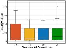
Figure 1: Bandwidths for models with different numbers of variables for the synthetic datasets.

We provide the consistency and the non-asymptotic sample complexity of $\hat{\mathbf{\Omega}}^{0}$ in Theorem 1.

Theorem 1.

Suppose that Assumptions 1–5 are satisfied. Given $n$ independent observations $\left\{\mathbf{z}^{i},g^{i}\right\}_{i\in[n]}$, we assume that there are $C_{1}>0$ and $C_{2}>0$, satisfying

$$\begin{split}\min_{\left\{j,j^{\prime}\>|\>\exists i\in[n],\Omega_{jj^{\prime}}(g^{i})\neq 0\right\}}&\sqrt{n^{-1}\sum_{i\in[n]}\left(\mathbf{\Omega}_{jj^{\prime}}(g^{i})\right)^{2}}\\ &\qquad\qquad\quad\leq C_{1}\sqrt{\log p}n^{-2/5},\end{split}$$

where $n\geq C_{2}d^{5/2}(\log p)^{5/4}$, and

$$\lambda=\frac{\left(C_{\mathbf{M}}+C_{\mathbf{R}}\right)}{C_{2}}\sqrt{(r+1)\log p-\log C_{1}}n^{-2/5},$$

where $d$ denotes the maximum node degree of the graph.

Then, for any $r>0$, we have

$$\begin{split}&\absolutevalue{\hat{\mathbf{\Omega}}^{0}-\mathbf{\Omega}^{0}}_{\infty}\\ \leq&\frac{3\left(C_{\mathbf{M}}+C_{\mathbf{R}}\right)^{2}}{C_{2}}\sqrt{(r+1)\log p-\log C_{1}}n^{-2/5}\\ &+\frac{C_{\mathbf{M}}}{\sqrt{2}}\sqrt{(r+2)\log p+\log 2}n^{-1/2},\end{split}$$ (8)

with probability larger than $1-2p^{-r}$.

In words, Theorem 1 indicates that, with a high probability, the estimation error is bounded by $O\left(\sqrt{\frac{\log p}{n^{4/5}}}\right)$. Inevitably, it is slightly larger than $O\left(\sqrt{\frac{\log p}{n}}\right)$, i.e, the non-asymptotic sample complexity of CLIME with $n$ i.i.d. data. Therefore, even in the presence of confounding, we can consistently and efficiently estimate the underlying precision matrix $\mathbf{\Omega}^{0}$ that encodes the true connectivity pattern, with a convergence rate comparable to CLIME without any confounding.

5.3 PROOF SKETCH

We provide a rough sketch idea on the proof for Theorem 1, and defer the details to the appendix.

To begin with, we need the following Lemma 1 on the convergence of $\mathbf{S}(g)$ to $\mathbf{\Sigma}(g)$, since the derived estimator $\hat{\mathbf{\Omega}}^{0}$ is highly dependent on the nonparametric estimator $\mathbf{S}(g)$.

Lemma 1.

Suppose that the Assumption 1 and Assumption 3 to 5 in Section 5.1 are satisfied, and that $C_{1}$ and $C_{2}$ are defined in Theorem 1. Then, for any $r>0$, and

$$\delta=\frac{\sqrt{(r+1)\log p-\log C_{1}}}{C_{2}}n^{-2/5},$$

the difference between $\mathbf{S}(g)$ and $\mathbf{\Sigma}(g)$ can be bounded in probability by

$$\begin{split}\Pr{\sup_{g}\absolutevalue{\mathbf{S}(g)-\mathbf{\Sigma}(g)}_{\infty}\geq\delta}\leq p^{-r}.\end{split}$$ (9)

Proof.

By following the rationale of the Lemma 8 in [64], we can derive

$$\begin{split}\Pr&\left\{\sup_{g}\absolutevalue{\mathbf{S}(g)-\mathbf{\Sigma}(g)}_{\infty}\geq\epsilon\right\}\\ &\leq C_{1}\exp(-C_{2}n^{4/5}\epsilon^{2}+\log p).\end{split}$$

Then, by letting $\epsilon=\sqrt{\frac{\log(p^{r+1}C_{1}^{-1})}{C_{2}n^{4/5}}}$, we complete the proof. ∎

Lemma 1 provides a uniform convergence result over $g$ of the local covariance estimator.

Then, instead of directly studying $\absolutevalue{\hat{\mathbf{\Omega}}^{0}-\mathbf{\Omega}^{0}}_{\infty}$, we start by bounding $\absolutevalue{\hat{\mathbf{\Omega}}^{0}-\mathbf{M}}_{\infty}$, where

$$\mathbf{M}=\frac{\sum_{i\in[n]}\mathbf{\Omega}(g^{i})}{n}.$$

Specifically, with Lemma 1, we derive Lemma 2 on the relationship between $\hat{\mathbf{\Omega}}^{0}$ and $\mathbf{M}$.

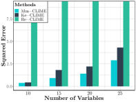
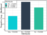
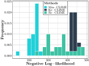
Figure 2: Squared error for the considered methods with the selected $\lambda$’s using synthetic datasets.

    Figure 3: Barplot of estimated negative log-likelihoods using the selected $\lambda$’s, histogram of the considered methods with all $\lambda$’s, using the COBRE dataset.

Figure 4: Glass brain figure of the estimated precision matrix using Mm-CLIME on the COBRE dataset (see manuscript for details).

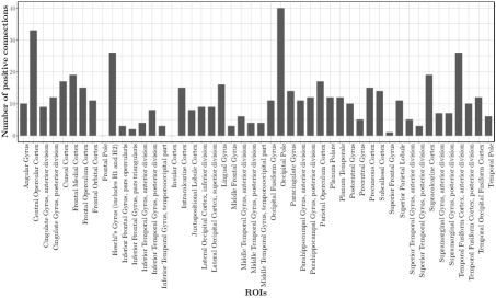
Figure 5: Number of positive connections across ROIs of the subjects diagnosed with schizophrenia recovered by the proposed Mm-CLIME method.

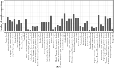
Figure 6: Number of positive connections across ROIs of the control subjects recovered by the proposed Mm-CLIME method.

Lemma 2.

Suppose that the conditions in Theorem 1 are satisfied. Then, for any $r>0$,

$$\begin{split}\absolutevalue{\hat{\mathbf{\Omega}}^{0}-\mathbf{M}}_{\infty}\qquad&\\ \qquad\leq\frac{3\left(C_{\mathbf{M}}+C_{\mathbf{R}}\right)^{2}}{C_{2}}&\sqrt{(r+1)\log p-\log C_{1}}n^{-2/5},\end{split}$$ (10)

with probability larger than $1-p^{-r}$.

The proof of Lemma 2 is deferred to the appendix.

Finally, we bound $\absolutevalue{\mathbf{M}-\mathbf{\Omega}^{0}}_{\infty}$. According to Lemma 2, $\hat{\mathbf{\Omega}}^{0}$ converges to $\mathbf{M}$. Therefore, we can prove the consistency of $\hat{\mathbf{\Omega}}^{0}$ by studying the relationship between $\mathbf{M}$ and $\mathbf{\Omega}^{0}$. Specifically, by Hoeffding inequality, we have

$$\Pr{\absolutevalue{\mathbf{\Omega}^{0}-\mathbf{M}}_{\infty}\geq C_{\mathbf{M}}\sqrt{\log(2p^{r+2})}(2n)^{-1/2}}\leq p^{-r},$$ (11)

for any $r>0$.

Combine (11) with Lemma 2, we have

$$\begin{split}&\absolutevalue{\hat{\mathbf{\Omega}}^{0}-\mathbf{\Omega}^{0}}_{\infty}\\ \leq&\frac{3\left(C_{\mathbf{M}}+C_{\mathbf{R}}\right)^{2}}{C_{2}}\sqrt{\log(p^{r+1})-\log(C_{1})}n^{-2/5}\\ &+\frac{C_{\mathbf{M}}}{\sqrt{2}}\sqrt{\log(p^{r+2})+\log(2)}n^{-1/2},\end{split}$$

with probability $1-2p^{-r}$.

6 EXPERIMENTS

In what follows, we will demonstrate that the proposed method efficiently recovers the target precision matrix when applied to synthetic data in Section 6.1. Then, to illustrate that the proposed model is readily applicable to practical analysis of brain connectivity, we apply it to a resting-state functional magnetic resonance imaging dataset collected for the study of schizophrenia.

6.1 SYNTHETIC EXPERIMENTS

In this section, we compare the proposed model with some existing models using synthetic data. Specifically, we consider a generative model where the underlying precision matrix varies smoothly with respect to the confounder variable $G$. Then, we generate samples with varying precision matrices via the following procedure:

1. We set the length of the multivariate random variable $\mathbf{Z}$ to $p=10,15,20,25$, and implement the following steps separately.

2. We randomly generate $11$ precision matrices as anchors, denoted by $\mathbf{\Omega}^{1},\mathbf{\Omega}^{11},\mathbf{\Omega}^{21},\mathbf{\Omega}^{31},\cdots,\mathbf{\Omega}^{101}$. Specifically, each element of the anchor precision matrices is drawn randomly to be non-zero with probability 0.2. The values of non-zero elements follow a uniform distribution.

3. Precision matrices between every two consecutive anchor precision matrices are constructed by linear interpolation.

4. For each precision matrix, we generate $2$ independent zero-mean multivariate Gaussian samples, which constitute the synthetic dataset, $\mathbb{Z}$.

5. We set the target precision matrix as $\mathbf{\Omega}^{0}=\frac{\sum_{i=1}^{101}\mathbf{\Omega}^{i}}{101}$, and the $\mathbf{\Omega}^{0}$ is thresholded for the sparsity.

6. The considered methods are applied to $\mathbb{Z}$ to estimate $\mathbf{\Omega}^{0}$.

Note that by following the procedure above, the simulated model is equivalent to a generative model with fixed precision $\mathbf{\Omega}^{0}$ and additive confounding $\mathbf{R}^{i}=\mathbf{\Omega}^{0}-\mathbf{\Omega}^{i}$, where the superscripts indicate the confounder variable $G$.

The proposed method is based on a movement modeling method, and thus is denoted by Mm-CLIME. According to the analysis in Section 2, the competing methods fall into three categories: the precision matrix estimation with confounding (which is designed exactly for our problem setting), time-varying precision matrix estimation [71, 27, 67, 31, 46, 32], and multiple precision matrix estimation [8, 21, 9, 48, 42]. We also study two benchmarks: Re-CLIME and Ke-CLIME from the first two categories.

The baseline Re-CLIME refers to the procedure that linearly regresses out the confounding by $G$ from the observed samples first, and then uses CLIME to estimate the precision matrix. As a precision matrix estimation method with confounding, Re-CLIME is widely applied to brain functional connectivity analysis in practice [62, 50]. Furthermore, we consider Ke-CLIME; a CLIME version of the method studied in [27] as a representative of time-varying precision matrix estimation. In this case, CLIME is separately applied to kernel estimators of the covariance matrix for each observation, which results in $101$ estimated precision matrices, i.e., estimates of the time-varying precision matrices. Then, we use the average of the precision matrices as an estimator of $\mathbf{\Omega}^{0}$.

To strike a fair comparison, we only select CLIME-based methods from each category of techniques. Otherwise, whether the efficiency gain of JNE comes from the joint estimation or CLIME will be unclear. Also, as suggested by [7], CLIME has at least comparable performance to the graphical Lasso.

Multiple precision matrix estimation methods are not included due to numerical issues. We observe that such methods require sufficient samples for the estimation of each precision matrix. Empirical evaluation of one such approach [42] most often resulted in ill-defined optimization problems, since we may have as few as two observations for each precision matrix.

The solutions obtained by the considered CLIME-based methods are not guaranteed to be symmetric or positive definite in general. To deal with this, a procedure provided in [7] is used to symmetrize solution of each method.

The Epanechnikov kernel is used with the bandwidth parameters selected by leave-one-out cross-validation. Since all the considered kernel-based methods use the same estimator of the covariance matrix, the same bandwidth are used across all the methods. Different bandwidths are used to estimate each component of the covariance matrix, resulting in $p(p-1)/2$ bandwidths. Values of these bandwidths are provided in Figure 1. The regularization parameters ($\lambda$’s) are determined by the Akaike information criterion (AIC). The selected $\lambda$’s are reported in Table 1.

The results are summarized in Figure 3. Notice that the proposed Mm-CLIME achieves the smallest squared error among all the considered methods. Furthermore, although Re-CLIME is widely used in practice to analyze the brain connectivity, it performs worst in terms of accuracy in our experiments. Actually, this is not surprising, since the effects of confounders on the observed data are seldom linear, both in our synthetic setting and practical problems.

Compared with Ke-CLIME, the proposed model adds an extra constraint in the optimization program and, as a result, it can better take advantage of the assumption $E(R^{i})=0$ and achieves more accurate estimation. The main intuition for this advantage is that with our procedure, we can choose a smaller bandwidth parameter $h$, which results in smaller bias and better performance compared to simple averaging. Note that when averaging the estimated $\Omega(g)$ over $g$ the bias due to kernel estimation does not get reduced. Furthermore, estimation of each individual $\Omega(g)$ requires a larger bandwidth, resulting in more bias.

6.2 fMRI EXPERIMENTS

Functional brain connectivity measures associations between brain areas, and are thought to reflect communication and coordination between spatially distant neuronal populations – corresponding to information processing pathways in the brain. There are a wide variety of techniques for estimating functional connectivity in the literature [53, 12, 70, 4], most commonly via the correlation. However, there is increasing evidence that the precision matrix results in a more stable and effective connectivity estimate than the alternatives [63, 49, 55, 56, 1]. For this reason, we focus our attention on precision matrix estimation. We also focus on motion confounding – one of the most pressing examples of physiological confounding in the literature.

Our experiments use data from the Center for Biomedical Research Excellence (COBRE). We compare the considered methods using preprocessed resting-state functional magnetic resonance images for $70$ patients diagnosed with schizophrenia, and $72$ healthy controls. Every patient has more than $150$ fMRI observations each with $22$ corresponding confounders. We use the $7$ confounders provided in the dataset related to motion for the analysis. Furthermore, we apply Harvard-Oxford Atlas to generate 48 atlas regions of interest (ROIs).

First we split the data from each patient into a training test with $70\%$ of the data and a test set with $30\%$ of the data. Then, we apply the method to training sets to estimate an unconfounded precision matrix for each patient. Further, we treat the observations of each test set as the samples of a multivariate normal distribution with the precision matrix as estimated, and calculate the log-likelihood to compare different methods. A glass brain figure illustrating the achieved precision matrix of a patient with schizophrenia is provided in Figure 4. Our hypothesis is that the confounding has a similar effect as additive noise. Thus, better estimation of the average precision will correspond to higher likelihood. The results using the $\lambda$ selected by AIC and the results using all considered $\lambda$’s are both summarized in Figure 3. As expected, we find that the proposed method achieves the highest log-likelihood on the held-out dataset, which suggests that it results in a better model of the brain connectivity than the baselines.

Next, we concatenated all the observations across subjects diagnosed with schizophrenia, and and all the healthy controls into two time series, then apply the proposed method separately to each concatenated time series. The results are summarized in Figure 5 and Figure 6, where the number of positive connections for each ROI are reported. We notice that the connectivity of the ROIs of the subjects with schizophrenia are similar to that of the control group, except the Occipital Pole and Central Opercular Cortex have abnormally more positive connections with other ROIs, i.e., most highly connected areas. Interestingly, these two areas have been implicated in the literature as highly associated with schizophrenia [54, 61]. In summary, the proposed method models the fMRI accurately, and detects the differences between the subjects with schizophrenia and the control group.

7 Conclusion

We developed a novel approach for precision matrix estimation where, due to extraneous confounding of the underlying precision matrix, the data are independent but not identically distributed. For this, we proposed a varying graphical model, and an associated joint nonparametric estimator. Our technical contributions included theoretical consistency and convergence rate guarantees for the proposed estimator, and an efficient optimization procedure. Empirical results were also presented using simulated and real brain imaging data, which suggests that our approach improves precision matrix estimation as compared to a variety of baselines. For future work, we plan to investigate more complex hierarchical graphical models including more confounder effects, and joint estimation across groups to better estimate shared global structure.

We have focused on the estimation of the precision matrix under a specific model of confounding. An interesting future direction is development of a goodness of fit test that would allow us to verify if the model specification is appropriate for data. Extending recent work on quantifying uncertainty in estimation of edge parameters in undirected graphical models [66, 52, 65, 3, 68, 26, 69, 25] to a setting with confounding is rather challenging and will be pursued elsewhere.

Empirical results were also presented suggesting an improvement for precision matrix estimation.

References

Supplements

Proof for Lemma 2

According to Lemma 1, for any $r>0$,

$$\begin{split}\sup_{g}\absolutevalue{\mathbf{S}(g)-\mathbf{\Sigma}(g)}_{\infty}\geq\sqrt{\log(p^{r+1}C_{1}^{-1})}C_{2}^{-1}n^{-2/5}\end{split}$$ (12)

with probability larger than $1-p^{-r}$.

For the ease of presentation, we now use $\mathbf{S}^{i}$ to denote $\mathbf{S}(g^{i})$ and $\mathbf{R}^{i}=\mathbf{\Omega}(g^{i})-\mathbf{M}$. Assuming that (12) holds, we can see that $\mathbf{M}$ and $\left\{\mathbf{R}^{i}\right\}_{i=1}^{n}$ is a pair of feasible solution to (5) for

$$\begin{split}\absolutevalue{\mathbf{I}-\mathbf{S}^{i}\left(\mathbf{M}+\mathbf{R}^{i}\right)}_{\infty}&=\absolutevalue{\left(\mathbf{\Sigma}(g^{i})-\mathbf{S}^{i}\right)\left(\mathbf{M}+\mathbf{R}^{i}\right)}_{\infty}\\ &\leq(C_{\mathbf{M}}+C_{\mathbf{R}})\sqrt{\log(p^{r+1}C_{1}^{-1})}C_{2}^{-1}n^{-2/5}\\ &=\lambda.\end{split}$$

Then, we consider $\absolutevalue{\sum_{i=1}^{n}\left(\mathbf{M}+\mathbf{R}^{i}-\hat{\mathbf{\Omega}}^{0}-\hat{\mathbf{R}}^{i}\right)\mathbf{e}_{j}}_{\infty}$, which satisfies :

$$\begin{split}\absolutevalue{\sum_{i=1}^{n}\left(\mathbf{M}+\mathbf{R}^{i}-\hat{\mathbf{M}}-\hat{\mathbf{R}}^{i}\right)\mathbf{e}_{j}}_{\infty}\leq&\absolutevalue{\sum_{i=1}^{n}\left(\mathbf{M}+\mathbf{R}^{i}\right)\left(\mathbf{\Sigma}^{i}-\mathbf{S}^{i}\right)\left(\hat{\mathbf{\Omega}}^{0}+\hat{\mathbf{R}}^{i}\right)\mathbf{e}_{j}}_{\infty}\\ &+\absolutevalue{\sum_{i=1}^{n}\left(\mathbf{M}+\mathbf{R}^{i}\right)\left(\mathbf{S}^{i}\left(\hat{\mathbf{\Omega}}^{0}+\hat{\mathbf{R}}^{i}\right)-\mathbf{I}\right)\mathbf{e}_{j}}_{\infty},\end{split}$$

where $\mathbf{I}$ is the identity matrix.

For $\absolutevalue{\sum_{i=1}^{n}\left(\mathbf{M}+\mathbf{R}^{i}\right)\left(\mathbf{\Sigma}(g^{i})-\mathbf{S}^{i}\right)\left(\hat{\mathbf{\Omega}}^{0}+\hat{\mathbf{R}}^{i}\right)\mathbf{e}_{j}}_{\infty}$, according to the Assumption 3, we have:

$$\begin{split}&\absolutevalue{\sum_{i=1}^{n}\left(\mathbf{M}+\mathbf{R}^{i}\right)\left(\mathbf{\Sigma}(g^{i})-\mathbf{S}^{i}\right)\left(\hat{\mathbf{\Omega}}^{0}+\hat{\mathbf{R}}^{i}\right)\mathbf{e}_{j}}_{\infty}\\ \leq&\norm{\mathbf{M}}\left\{\sum_{i=1}^{n}\absolutevalue{\mathbf{\Sigma}(g^{i})-\mathbf{S}^{i}}_{\infty}\absolutevalue{\hat{\bm{\omega}}_{j}}_{1}+\sum_{i=1}^{n}\absolutevalue{\mathbf{\Sigma}(g^{i})-\mathbf{S}^{k}}_{\infty}\absolutevalue{\hat{\mathbf{r}}^{i}_{j}}_{1}\right\}\\ &+\sum_{i=1}^{n}\norm{\mathbf{R}^{i}}_{L_{1}}\absolutevalue{\left(\mathbf{\Sigma}(g^{i})-\mathbf{S}^{i}\right)}_{\infty}\absolutevalue{\hat{\bm{\omega}}_{j}}_{1}+\sum_{i=1}^{n}\norm{\mathbf{R}^{i}}_{L_{1}}\absolutevalue{\left(\mathbf{\Sigma}^{i}-\mathbf{S}^{i}\right)}_{\infty}\absolutevalue{\hat{\mathbf{r}}^{i}_{j}}_{1}\\ \leq&C_{\mathbf{M}}\left\{n\max_{i}\absolutevalue{\left(\mathbf{\Sigma}(g^{i})-\mathbf{S}^{i}\right)}_{\infty}\absolutevalue{\hat{\bm{\omega}}_{j}}_{1}+\max_{i}\absolutevalue{\left(\mathbf{\Sigma}(g^{i})-\mathbf{S}^{k}\right)}_{\infty}\sum_{i=1}^{n}\absolutevalue{\hat{\mathbf{r}}^{i}_{j}}_{1}\right\}\\ &+\absolutevalue{\hat{\bm{\omega}}_{j}}_{1}\max_{i}\absolutevalue{\left(\mathbf{\Sigma}(g^{i})-\mathbf{S}^{i}\right)}_{\infty}\sum_{i=1}^{n}\norm{\mathbf{R}^{i}}_{L_{1}}+\max_{i}\absolutevalue{\left(\mathbf{\Sigma}(g^{i})-\mathbf{S}^{i}\right)}_{\infty}\sum_{i=1}^{n}\norm{\mathbf{R}^{i}}_{L_{1}}\absolutevalue{\hat{\mathbf{r}}^{i}_{j}}_{1}\\ \leq&C_{\mathbf{M}}\sqrt{\log(p^{r+1}C_{1}^{-1})}C_{2}^{-1}n^{3/5}\absolutevalue{\hat{\bm{\omega}}_{j}}_{1}+C_{\mathbf{M}}\sqrt{\log(p^{r+1}C_{1}^{-1})}C_{2}^{-1}n^{-2/5}\sum_{i=1}^{n}\absolutevalue{\hat{\mathbf{r}}_{j}^{i}}_{1}\\ &+C_{\mathbf{R}}\sqrt{\log(p^{r+1}C_{1}^{-1})}C_{2}^{-1}n^{3/5}\absolutevalue{\hat{\bm{\omega}}_{j}}_{1}+C_{\mathbf{R}}\sqrt{\log(p^{r+1}C_{1}^{-1})}C_{2}^{-1}n^{-2/5}\sum_{i=1}^{n}\absolutevalue{\hat{\mathbf{r}}_{j}^{i}}_{1}\\ =&2\left(C_{\mathbf{M}}+C_{\mathbf{R}}\right)\sqrt{\log(p^{r+1}C_{1}^{-1})}C_{2}^{-1}n^{3/5}\left(\absolutevalue{\hat{\bm{\omega}}_{j}}_{1}+\frac{\sum_{i=1}^{n}\absolutevalue{\hat{\mathbf{r}}_{j}^{i}}_{1}}{n}\right),\end{split}$$

where $\hat{\bm{\omega}}_{j}$ denotes the $j$th column of $\hat{\mathbf{\Omega}}^{0}$

Since $\mathbf{M}$ and $\left\{\mathbf{R}^{i}\right\}_{i=1}^{n}$ is a set of feasible solution to (5), combined with the definition of (5), we can derive the upperbound of $\absolutevalue{\sum_{i=1}^{n}\left(\mathbf{M}+\mathbf{R}^{i}\right)\left(\mathbf{\Sigma}(g^{i})-\mathbf{S}^{i}\right)\left(\hat{\mathbf{\Omega}}^{0}+\hat{\mathbf{R}}^{i}\right)\mathbf{e}_{j}}_{\infty}$ as:

$$\begin{split}&\absolutevalue{\sum_{i=1}^{n}\left(\mathbf{M}+\mathbf{R}^{i}\right)\left(\mathbf{\Sigma}(g^{i})-\mathbf{S}^{i}\right)\left(\hat{\mathbf{\Omega}}^{0}+\hat{\mathbf{R}}^{i}\right)\mathbf{e}_{j}}_{\infty}\\ \leq&2\left(C_{\mathbf{M}}+C_{\mathbf{R}}\right)\sqrt{\log(p^{r+1}C_{1}^{-1})}C_{2}^{-1}n^{3/5}\left(\absolutevalue{\hat{\bm{\omega}}_{j}}_{1}+\frac{\sum_{i=1}^{n}\absolutevalue{\hat{\mathbf{r}}_{j}^{i}}_{1}}{n}\right)\\ \leq&2\left(C_{\mathbf{M}}+C_{\mathbf{R}}\right)^{2}\sqrt{\log(p^{r+1}C_{1}^{-1})}C_{2}^{-1}n^{3/5},\end{split}$$ (13)

where the second inequality is due to the Assumption 3.

Furthermore, for $\absolutevalue{\sum_{i=1}^{n}\left(\mathbf{M}+\mathbf{R}^{i}\right)\left(\mathbf{S}^{i}\left(\hat{\mathbf{\Omega}}^{0}+\hat{\mathbf{R}}^{i}\right)-\mathbf{I}\right)\mathbf{e}_{j}}_{\infty}$, we have:

$$\begin{split}&\absolutevalue{\sum_{i=1}^{n}\left(\mathbf{M}+\mathbf{R}^{i}\right)\left(\mathbf{S}^{i}\left(\hat{\mathbf{\Omega}}^{0}+\hat{\mathbf{R}}^{i}\right)-\mathbf{I}\right)\mathbf{e}_{j}}_{\infty}\\ \leq&\norm{\mathbf{M}}_{L_{1}}\absolutevalue{\sum_{i=1}^{n}\left(\mathbf{S}^{i}\left(\hat{\mathbf{\Omega}}^{0}+\hat{\mathbf{R}}^{i}\right)-\mathbf{I}\right)\mathbf{e}_{j}}_{\infty}+\sum_{i=1}^{n}\norm{\mathbf{R}^{i}}_{L_{1}}\absolutevalue{\left(\mathbf{S}^{i}\left(\hat{\mathbf{\Omega}}^{0}+\hat{\mathbf{R}}^{i}\right)-\mathbf{I}\right)\mathbf{e}_{j}}_{\infty}\\ \leq&\lambda\left(\norm{\mathbf{M}}_{L_{1}}+\sum_{i=1}^{n}\norm{\mathbf{R}^{i}}_{L_{1}}\right)\\ =&(nC_{\mathbf{R}}+C_{\mathbf{M}})(C_{\mathbf{M}}+C_{\mathbf{R}})\sqrt{\log(p^{r+1}C_{1}^{-1})}C_{2}^{-1}n^{-2/5}.\end{split}$$ (14)

Therefore, combining (13) and (14), we can prove the consistency of $\hat{\mathbf{\Omega}}^{0}$ by

$$\begin{split}&\frac{\absolutevalue{\sum_{i=1}^{n}\left(\mathbf{M}+\mathbf{R}^{i}-\hat{\mathbf{\Omega}}^{0}-\hat{\mathbf{R}}^{i}\right)\mathbf{e}_{j}}_{\infty}}{n}\\ =&\absolutevalue{\hat{\mathbf{\Omega}}^{0}-\mathbf{M}}_{\infty}\\ \leq&\left(C_{\mathbf{M}}+C_{\mathbf{R}}\right)\left(3C_{\mathbf{R}}+(2+n^{-1})C_{\mathbf{M}}\right)\sqrt{\log(p^{r+1}C_{1}^{-1})}C_{2}^{-1}n^{-2/5},\end{split}$$ (15)

with probability larger than $1-p^{-r}$.

References

- Andersen et al. [2018] M. Andersen, O. Winther, L. K. Hansen, R. Poldrack, and O. Koyejo. Bayesian structure learning for dynamic brain connectivity. In AISTATS, 2018.
- Arbabshirani and Calhoun [2011] M. R. Arbabshirani and V. D. Calhoun. Functional network connectivity during rest and task: comparison of healthy controls and schizophrenic patients. In EMBC, 2011.
- Barber and Kolar [2018] R. F. Barber and M. Kolar. Rocket: Robust confidence intervals via kendall’s tau for transelliptical graphical models. Ann. Statist., 46(6B):3422–3450, 2018.
- Barch et al. [2013] D. M. Barch, G. C. Burgess, M. P. Harms, S. E. Petersen, B. L. Schlaggar, M. Corbetta, M. F. Glasser, S. Curtiss, S. Dixit, C. Feldt, et al. Function in the human connectome: task-fmri and individual differences in behavior. Neuroimage, 80:169–189, 2013.
- Biswal et al. [1995] B. Biswal, F. Zerrin Yetkin, V. M. Haughton, and J. S. Hyde. Functional connectivity in the motor cortex of resting human brain using echo-planar mri. Magnetic resonance in medicine, 34(4):537–541, 1995.
- Caballero-Gaudes and Reynolds [2017] C. Caballero-Gaudes and R. C. Reynolds. Methods for cleaning the bold fmri signal. Neuroimage, 154:128–149, 2017.
- Cai et al. [2011] T. T. Cai, W. Liu, and X. Luo. A constrained minimization approach to sparse precision matrix estimation. J. Am. Stat. Assoc., 106(494):594–607, 2011.
- Chiquet et al. [2011] J. Chiquet, Y. Grandvalet, and C. Ambroise. Inferring multiple graphical structures. Stat. Comput., 21(4):537–553, 2011.
- Danaher et al. [2014] P. Danaher, P. Wang, and D. M. Witten. The joint graphical lasso for inverse covariance estimation across multiple classes. J. R. Stat. Soc. B, 76(2):373–397, 2014.
- Drton and Maathuis [2017] M. Drton and M. H. Maathuis. Structure learning in graphical modeling. Annual Review of Statistics and Its Application, 4(1):365–393, 2017.
- Evgeniou and Pontil [2004] T. Evgeniou and M. Pontil. Regularized multi-task learning. In SIGKDD, 2004.
- Fornito et al. [2013] A. Fornito, A. Z. Lee, and M. Breakspear. Graph analysis of the human connectome: Promise, progress, and pitfalls. NeuroImage, 80:426–444, 2013.
- Fox and Raichle [2007] M. D. Fox and M. E. Raichle. Spontaneous fluctuations in brain activity observed with functional magnetic resonance imaging. Nature Reviews Neuroscience, 8(9):700–711, 2007.
- Friedman et al. [2008] J. H. Friedman, T. J. Hastie, and R. J. Tibshirani. Sparse inverse covariance estimation with the graphical lasso. Biostatistics, 9(3):432–441, 2008.
- Friedman [2004] N. Friedman. Inferring cellular networks using probabilistic graphical models. Science, 303(5659):799–805, 2004.
- Geng et al. [2017] S. Geng, Z. Kuang, and D. Page. An efficient pseudo-likelihood method for sparse binary pairwise markov network estimation. arXiv:1702.08320, 2017.
- Geng et al. [2018a] S. Geng, Z. Kuang, J. Liu, S. Wright, and D. Page. Stochastic learning for sparse discrete markov random fields with controlled gradient approximation error. In UAI, 2018a.
- Geng et al. [2018b] S. Geng, Z. Kuang, P. Peissig, and D. Page. Temporal poisson square root graphical models. In ICML, 2018b.
- Geng et al. [2019] S. Geng, M. Yan, M. Kolar, and S. Koyejo. Partially linear additive Gaussian graphical models. In ICML 36, 2019.
- Goto et al. [2016] M. Goto, O. Abe, T. Miyati, H. Yamasue, T. Gomi, and T. Takeda. Head motion and correction methods in resting-state functional mri. Magnetic Resonance in Medical Sciences, 15(2):178–186, 2016.
- Guo et al. [2011] J. Guo, E. Levina, G. Michailidis, and J. Zhu. Joint estimation of multiple graphical models. Biometrika, 98(1):1–15, 2011.
- Gurobi Optimization [2016] I. Gurobi Optimization. Gurobi optimizer reference manual, 2016.
- Hong et al. [2012] L. Hong, A. Ahmed, S. Gurumurthy, A. J. Smola, and K. Tsioutsiouliklis. Discovering geographical topics in the twitter stream. In WWW 21, 2012.
- Hsieh et al. [2013] C.-J. Hsieh, M. A. Sustik, I. S. Dhillon, P. K. Ravikumar, and R. Poldrack. Big & quic: Sparse inverse covariance estimation for a million variables. In NIPS, 2013.
- Janková and van de Geer [2019] J. Janková and S. van de Geer. Inference in high-dimensional graphical models. In Handbook of graphical models, Chapman & Hall/CRC Handb. Mod. Stat. Methods, pages 325–349. CRC Press, Boca Raton, FL, 2019.
- Kim et al. [2019] B. Kim, S. Liu, and M. Kolar. Two-sample inference for high-dimensional markov networks. arXiv 1905.00466, 2019.
- Kolar and Xing [2011] M. Kolar and E. P. Xing. On time varying undirected graphs. In AISTATS, 2011.
- Kolar and Xing [2012] M. Kolar and E. P. Xing. Estimating networks with jumps. Electron. J. Stat., 6:2069–2106, 2012.
- Kolar et al. [2009a] M. Kolar, L. Song, and E. P. Xing. Sparsistent learning of varying-coefficient models with structural changes. In Y. Bengio, D. Schuurmans, J. D. Lafferty, C. K. I. Williams, and A. Culotta, editors, NIPS, pages 1006–1014, 2009a.
- Kolar et al. [2009b] M. Kolar, L. Song, and E. P. Xing. Sparsistent learning of varying-coefficient models with structural changes. In NIPS, 2009b.
- Kolar et al. [2010a] M. Kolar, A. P. Parikh, and E. P. Xing. On sparse nonparametric conditional covariance selection. In J. Fürnkranz and T. Joachims, editors, 27th Int. Conf. Mach. Learn., Haifa, Israel, 2010a.
- Kolar et al. [2010b] M. Kolar, L. Song, A. Ahmed, and E. P. Xing. Estimating Time-varying networks. Ann. Appl. Stat., 4(1):94–123, 2010b.
- Kolar et al. [2013] M. Kolar, H. Liu, and E. P. Xing. Markov network estimation from multi-attribute data. In ICML, 2013.
- Kolar et al. [2014] M. Kolar, H. Liu, and E. P. Xing. Graph estimation from multi-attribute data. J. Mach. Learn. Res., 15(1):1713–1750, 2014.
- Kuang et al. [2016a] Z. Kuang, J. Thomson, M. Caldwell, P. Peissig, R. Stewart, and D. Page. Baseline regularization for computational drug repositioning with longitudinal observational data. In IJCAI, 2016a.
- Kuang et al. [2016b] Z. Kuang, J. Thomson, M. Caldwell, P. Peissig, R. Stewart, and D. Page. Computational drug repositioning using continuous self-controlled case series. In SIGKDD, 2016b.
- Kuang et al. [2017a] Z. Kuang, S. Geng, and D. Page. A screening rule for l1-regularized ising model estimation. In NIPS, 2017a.
- Kuang et al. [2017b] Z. Kuang, P. Peissig, V. Santos Costa, R. Maclin, and D. Page. Pharmacovigilance via baseline regularization with large-scale longitudinal observational data. In SIGKDD, 2017b.
- Laumann et al. [2016] T. O. Laumann, A. Z. Snyder, A. Mitra, E. M. Gordon, C. Gratton, B. Adeyemo, A. W. Gilmore, S. M. Nelson, J. J. Berg, D. J. Greene, et al. On the stability of bold fmri correlations. Cerebral cortex, 27(10):4719–4732, 2016.
- Lauritzen [1996] S. L. Lauritzen. Graphical Models, volume 17 of Oxford Statistical Science Series. The Clarendon Press Oxford University Press, New York, 1996. Oxford Science Publications.
- Lee and Hastie [2015] J. D. Lee and T. J. Hastie. Learning the structure of mixed graphical models. J. Comput. Graph. Statist., 24(1):230–253, 2015.
- Lee and Liu [2015] W. Lee and Y. Liu. Joint estimation of multiple precision matrices with common structures. J. Mach. Learn. Res., 16:1035–1062, 2015.
- Li et al. [2013] Q. Li, J. Lin, and J. S. Racine. Optimal bandwidth selection for nonparametric conditional distribution and quantile functions. J. Bus. Econom. Statist., 31(1):57–65, 2013.
- Liu et al. [2014] J. Liu, C. Zhang, E. S. Burnside, and D. Page. Multiple testing under dependence via semiparametric graphical models. In ICML, pages 955–963, 2014.
- Liu et al. [2016] J. Liu, C. Zhang, and D. Page. Multiple testing under dependence via graphical models. Ann. Appl. Stat., 10(3):1699–1724, 2016.
- Lu et al. [2018] J. Lu, M. Kolar, and H. Liu. Post-regularization inference for time-varying nonparanormal graphical models. J. Mach. Learn. Res., 18(203):1–78, 2018.
- Mignotte et al. [2000] M. Mignotte, C. Collet, P. Perez, and P. Bouthemy. Sonar image segmentation using an unsupervised hierarchical mrf model. IEEE transactions on image processing, 9(7):1216–1231, 2000.
- Mohan et al. [2014] K. Mohan, P. London, M. Fazel, D. M. Witten, and S.-I. Lee. Node-based learning of multiple gaussian graphical models. J. Mach. Learn. Res., 15:445–488, 2014.
- Poldrack et al. [2015] R. A. Poldrack, T. O. Laumann, O. Koyejo, B. Gregory, A. Hover, M.-Y. Chen, K. J. Gorgolewski, J. Luci, S. J. Joo, R. L. Boyd, et al. Long-term neural and physiological phenotyping of a single human. Nature communications, 6:8885, 2015.
- Power et al. [2014] J. D. Power, A. Mitra, T. O. Laumann, A. Z. Snyder, B. L. Schlaggar, and S. E. Petersen. Methods to detect, characterize, and remove motion artifact in resting state fMRI. NeuroImage, 84:320–341, 2014.
- Price et al. [2014] T. Price, C.-Y. Wee, W. Gao, and D. Shen. Multiple-network classification of childhood autism using functional connectivity dynamics. In International Conference on Medical Image Computing and Computer-Assisted Intervention, pages 177–184. Springer, 2014.
- Ren et al. [2015] Z. Ren, T. Sun, C.-H. Zhang, and H. H. Zhou. Asymptotic normality and optimalities in estimation of large Gaussian graphical models. Ann. Stat., 43(3):991–1026, 2015.
- Sadaghiani and Kleinschmidt [2013] S. Sadaghiani and A. Kleinschmidt. Functional interactions between intrinsic brain activity and behavior. Neuroimage, 80:379–386, 2013.
- Sheffield et al. [2015] J. M. Sheffield, G. Repovs, M. P. Harms, C. S. Carter, J. M. Gold, A. W. MacDonald III, J. D. Ragland, S. M. Silverstein, D. Godwin, and D. M. Barch. Fronto-parietal and cingulo-opercular network integrity and cognition in health and schizophrenia. Neuropsychologia, 73:82–93, 2015.
- Shine et al. [2015] J. M. Shine, O. Koyejo, P. T. Bell, K. J. Gorgolewski, M. Gilat, and R. A. Poldrack. Estimation of dynamic functional connectivity using multiplication of temporal derivatives. NeuroImage, 122:399–407, 2015.
- Shine et al. [2016] J. M. Shine, O. Koyejo, and R. A. Poldrack. Temporal metastates are associated with differential patterns of time-resolved connectivity, network topology, and attention. PNAS, 113(35):9888–9891, 2016.
- Song et al. [2009a] L. Song, M. Kolar, and E. P. Xing. Keller: Estimating time-varying interactions between genes. Bioinformatics, 25(12):i128–i136, 2009a.
- Song et al. [2009b] L. Song, M. Kolar, and E. P. Xing. Time-varying dynamic bayesian networks. In Y. Bengio, D. Schuurmans, J. D. Lafferty, C. K. I. Williams, and A. Culotta, editors, NIPS, pages 1732–1740, 2009b.
- Suggala et al. [2017] A. S. Suggala, M. Kolar, and P. Ravikumar. The Expxorcist: Nonparametric graphical models via conditional exponential densities. In NIPS 30, 2017.
- Sun et al. [2015] S. Sun, M. Kolar, and J. Xu. Learning structured densities via infinite dimensional exponential families. In NIPS 28, 2015.
- Tohid et al. [2015] H. Tohid, M. Faizan, and U. Faizan. Alterations of the occipital lobe in schizophrenia. Neurosciences, 20(3):213, 2015.
- Van Dijk et al. [2012] K. R. Van Dijk, M. R. Sabuncu, and R. L. Buckner. The influence of head motion on intrinsic functional connectivity mri. Neuroimage, 59(1):431–438, 2012.
- Varoquaux et al. [2010] G. Varoquaux, A. Gramfort, J.-B. Poline, and B. Thirion. Brain covariance selection: Better individual functional connectivity models using population prior. In NIPS, 2010.
- Wang and Kolar [2014] J. Wang and M. Kolar. Inference for sparse conditional precision matrices. arXiv:1412.7638, 2014.
- Wang and Kolar [2016] J. Wang and M. Kolar. Inference for high-dimensional exponential family graphical models. In AISTATS, 2016.
- Wasserman et al. [2014] L. A. Wasserman, M. Kolar, and A. Rinaldo. Berry-Esseen bounds for estimating undirected graphs. Electron. J. Stat., 8:1188–1224, 2014.
- Yin et al. [2010] J. Yin, Z. Geng, R. Li, and H. Wang. Nonparametric covariance model. Stat. Sinica, 20:469–479, 2010.
- Yu et al. [2016] M. Yu, V. Gupta, and M. Kolar. Statistical inference for pairwise graphical models using score matching. In NIPS 29, 2016.
- Yu et al. [2019] M. Yu, V. Gupta, and M. Kolar. Simultaneous inference for pairwise graphical models with generalized score matching. arXiv 1905.06261, 2019.
- Zalesky et al. [2012] A. Zalesky, A. Fornito, and E. Bullmore. On the use of correlation as a measure of network connectivity. Neuroimage, 60(4):2096–2106, 2012.
- Zhou et al. [2010] S. Zhou, J. D. Lafferty, and L. A. Wasserman. Time varying undirected graphs. Mach. Learn., 80(2-3):295–319, 2010.