Isolating the confining color field in the SU(3) flux tube

Abstract

Using lattice Monte Carlo simulations of SU(3) pure gauge theory, we determine the spatial distribution of all components of the color fields created by a static quark and antiquark. We identify the components of the measured chromoelectric field transverse to the line connecting the quark-antiquark pair with the transverse components of an effective Coulomb-like field $\vec{E}^{C}$ associated with the quark sources. Subtracting $\vec{E}^{C}$ from the total simulated chromoelectric field $\vec{E}$ yields a non-perturbative, primarily longitudinal chromoelectric field $\vec{E}^{NP}$, which we identify as the confining field. This is the first time that the chromoelectric field has been separated into perturbative and nonperturbative components, creating a new tool to study the color field distribution between a quark and an antiquark, and thus the long distance force between them.

1 Introduction

Quantum chromodynamics (QCD), the theory of the strong interactions describing the dynamics of quarks and gluons, has yet to provide a theoretical explanation of the experimentally established phenomenon of confinement, i.e., the confinement of quarks and gluons inside hadrons. Several mechanisms of confinement have been proposed (for a review, see Refs. greensite2011introduction ; Diakonov:2009jq ), each with its own merits and limitations, but a comprehensive picture is still missing. In particular, it is not yet clear which feature of QCD is responsible for the area-law behavior of Wilson loops that implies a linear confining potential between a static quark and antiquark at large distances. Results from numerical simulations have shown this linear potential for $q\bar{q}$ distances $\gtrsim$ 0.5 fm, and up to distances of about 1.4 fm in presence of dynamical quarks, where string breaking should take place Philipsen:1998de ; Kratochvila:2002vm ; Bali:2005fu .

A wealth of numerical analyses of SU(2) and SU(3) Yang-Mills theory Fukugita:1983du ; Kiskis:1984ru ; Flower:1985gs ; Wosiek:1987kx ; DiGiacomo:1989yp ; DiGiacomo:1990hc ; Cea:1992sd ; Matsubara:1993nq ; Cea:1994ed ; Cea:1995zt ; Bali:1994de ; Skala:1996ar ; Haymaker:2005py ; D'Alessandro:2006ug ; Cardaci:2010tb ; Cea:2012qw ; Cea:2013oba ; Cea:2014uja ; Cea:2014hma ; Cardoso:2013lla ; Caselle:2014eka ; Cea:2017ocq ; Shuryak:2018ytg have found that the dominant color field generated by a static quark-antiquark pair is the component of the chromoelectric field along the line connecting the pair. (See, in particular, the SU(2) studies of Ref. Cea:1995zt .) This longitudinal field results in tube-like structures (flux tubes) that naturally give rise to a long-distance linear quark-antiquark potential  Bander:1980mu ; Greensite:2003bk ; Ripka:2005cr ; Simonov:2018cbk .

The aim of this paper is to measure the complete color field distributions generating this heavy quark potential. To do this, we first perform a series of new simulations in SU(3) pure gauge theory, measuring all six components of the color electric and magnetic fields on all transverse planes passing through the line between the quarks. These simulations have been carried out for three values of the quark-antiquark separation, and they provide maps of the chromodynamic fields permeating the space between a quark and antiquark. (These fields can be viewed as analogous to the electromagnetic field permeating the space between a pair of oppositely charged particle obtained by the solution of Maxwell’s equations.)

We find that the chromomagnetic field is everywhere much smaller than the chromoelectric field. We then fit the measured transverse components of the chromoelectric field to an effective Coulomb-like field generated by sources at the positions of the quarks. A nonperturbative, mostly longitudinal, chromoelectric field is then obtained by subtracting the effective Coulomb-like field from the total chromoelectric field, thereby isolating its confining part. To the extent that the nonperturbative field generates the measured linear term in the long distance heavy quark potential, and the effective Coulomb-like field generates the measured Coulomb correction to the force, we will have gained new understanding into the development of the long distance force between a quark and an antiquark in terms of the color fields permeating the space between them.

2 Theoretical background and lattice observables

The field configurations generated by a static $q\bar{q}$ pair can be probed by calculating on the lattice the vacuum expectation value of the following connected correlation function DiGiacomo:1989yp ; DiGiacomo:1990hc ; Kuzmenko:2000bq ; DiGiacomo:2000va :

$$\rho_{W,\,\mu\nu}^{\rm conn}=\frac{\left\langle{\rm tr}\left(WLU_{P}L^{\dagger}\right)\right\rangle}{\left\langle{\rm tr}(W)\right\rangle}-\frac{1}{N}\,\frac{\left\langle{\rm tr}(U_{P}){\rm tr}(W)\right\rangle}{\left\langle{\rm tr}(W)\right\rangle}\;.$$ (1)

Here $U_{P}=U_{\mu\nu}(x)$ is the plaquette in the $(\mu,\nu)$ plane, connected to the Wilson loop $W$ by a Schwinger line $L$, and $N$ is the number of colors (see Fig. 1).

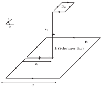
(a)                       

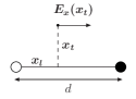
Figure 1:  1(a) The connected correlator given in Eq. (1) between the plaquette $U_{P}$ and the Wilson loop (subtraction in $\rho_{W,\,\mu\nu}^{\rm conn}$ not explicitly drawn).  1 The longitudinal chromoelectric field $E_{x}(x_{t})$ relative to the position of the static sources (represented by the white and black circles), for a given value of the transverse distance $x_{t}$.

The correlation function defined in Eq. (1) measures the field strength $F_{\mu\nu}$, since in the naive continuum limit DiGiacomo:1990hc

$$\rho_{W,\,\mu\nu}^{\rm conn}\stackrel{{\scriptstyle a\rightarrow 0}}{{\longrightarrow}}a^{2}g\left[\left\langle F_{\mu\nu}\right\rangle_{q\bar{q}}-\left\langle F_{\mu\nu}\right\rangle_{0}\right]\;,$$ (2)

where $\langle\quad\rangle_{q\bar{q}}$ denotes the average in the presence of a static $q\bar{q}$ pair, and $\langle\quad\rangle_{0}$ is the vacuum average. This relation is a necessary consequence of the gauge-invariance of the operator defined in Eq. (1) and of its linear dependence on the color field in the continuum limit (see Ref. Cea:2015wjd ).

The lattice definition of the quark-antiquark field-strength tensor $F_{\mu\nu}$ is then obtained by equating the two sides of Eq. (2) for finite lattice spacing. In the particular case when the Wilson loop $W$ lies in the plane with $\hat{\mu}=\hat{4}$ and $\hat{\nu}=\hat{1}$ (see Fig. 1(a)) and the plaquette $U_{P}$ is placed in the planes $\hat{4}\hat{1}$, $\hat{4}\hat{2}$, $\hat{4}\hat{3}$, $\hat{2}\hat{3}$, $\hat{3}\hat{1}$, $\hat{1}\hat{2}$, we get, respectively, the color field components $E_{x}$, $E_{y}$, $E_{z}$, $B_{x}$, $B_{y}$, $B_{z}$, at the spatial point corresponding to the position of the center of the plaquette, up to a sign depending on the orientation of the plaquette. Because of the symmetry of Fig. 1, the color fields take on the same values at spatial points connected by rotations around the axis on which the sources are located (the $\hat{1}$- or $x$-axis in the given example) .

As far as the color structure of the field $F_{\mu\nu}$ is concerned, we note that the source of $F_{\mu\nu}$ is the Wilson loop connected to the plaquette in Fig. 1. The role of the Schwinger lines entering in Eq. (1) is to realize the color parallel transport between the source loop and the “probe" plaquette. The Wilson loop defines a direction in color space. The color field, Eq. (2), that we measure points in a color direction parallel to this direction, the color direction of the source. (There are fluctuations of the color fields in the other color directions. These should contribute to the width of the energy density.)

In principle, the operator in Eq. (1) could be affected by $x_{t}$-dependent renormalization effects, related to Schwinger lines, which might contaminate the $x_{t}$ dependence of the color fields. However, our data satisfy continuum scaling; as carefully checked in Ref. Cea:2017ocq , fields obtained in the same physical setup, but at different values of beta, are in perfect agreement in the range of parameters used in the present work. This would have been impossible in the presence of sizeable renormalization effects. The absence of such effects is probably explained by the fact that we perform smearing before taking measurements (see below), and smearing effectively amounts to pushing the system towards the continuum, where renormalization effects become negligible.

In A we present some further discussion about the smearing procedure and, in particular, compare it with the approach based on the explicit renormalization of the operator given in (1), recently pursued in Ref. Battelli:2019lkz .

3 Lattice setup

We performed all simulations in pure gauge SU(3), with the standard Wilson action as the lattice discretization. A summary of the runs performed is given in Table 1. The error analysis was performed by the jackknife method over bins at different blocking levels.

Table 1: Summary of the runs performed in the SU(3) pure gauge theory (measurements are taken every 100 upgrades of the lattice configuration).

$\beta$	lattice	$a$[fm]	$d$ [lattice]	$d$ [fm]	statistics	smearing steps
6.370	$48^{4}$	0.059	16	0.951(11)	5300	100
6.240	$48^{4}$	0.071	16	1.142(15)	21000	100
6.136	$48^{4}$	0.083	16	1.332(20)	84000	120

We set the physical scale for the lattice spacing by using the value $\sqrt{\sigma}=420~{}$MeV for the string tension, and the parameterization Edwards:1998xf for $a\sqrt{\sigma}$ that gave an accurate fit in a high-statistics simulation for all $\beta$ in the range $5.6\leq\beta\leq 6.5$. The correspondences between $\beta$ and the distance $d$ shown in Table 1 were obtained from this parameterization. Note that the distance in lattice units between quark and antiquark, corresponding to the size of the Wilson loop in the connected correlator in Eq. (1), was kept fixed to $d=16\,a$.

The connected correlator defined in Eq. (1) suffers from large fluctuations at the scale of the lattice spacing, which are responsible for a bad signal-to-noise ratio. To extract the physical information carried by fluctuations at the physical scale (and, therefore, at large distances in lattice units) we smoothed out configurations by a smearing procedure. Our setup consisted of (just) one step of HYP smearing Hasenfratz:2001hp on the temporal links, with smearing parameters $(\alpha_{1},\alpha_{2},\alpha_{3})=(1.0,0.5,0.5)$, and $N_{\rm APE}$ steps of APE smearing Falcioni1985624 on the spatial links, with smearing parameter $\alpha_{\rm APE}=0.25$. Here $\alpha_{\rm APE}$ is the ratio of the weight of one staple to the weight of the original link.

4 Numerical results

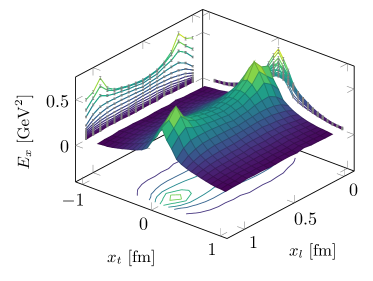
(a) $E_{x}(x_{t},x_{l})$

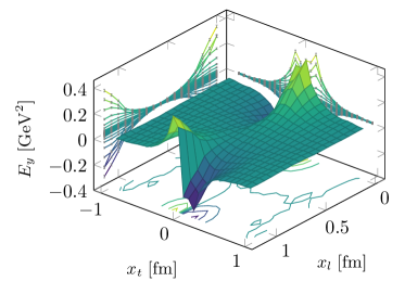
(b) $E_{y}(x_{t},x_{l})$

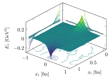
(c) $E_{z}(x_{t},x_{l})$

Figure 2: Surface and contour plots for the three components of the chromoelectric field at $\beta=6.240$ and $d=1.142$ fm. All plotted quantities are in physical units.

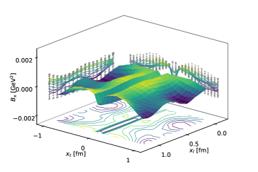
(a) $B_{x}(x_{t},x_{l})$

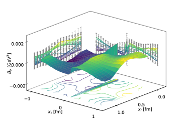
(b) $B_{y}(x_{t},x_{l})$

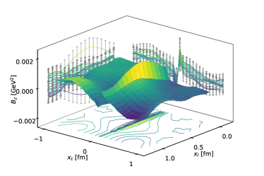
(c) $B_{z}(x_{t},x_{l})$

Figure 3: Surface and contour plots for the three components of the chromomagnetic field at $\beta=6.240$ and $d=1.142$ fm. All plotted quantities are in physical units.

Using Monte Carlo evaluations of the expectation value of the operator $\rho_{W,\,\mu\nu}^{\rm conn}$ over smeared ensembles, we have determined the six components of the color fields on all two-dimensional planes transverse to the line joining the color sources allowed by the lattice discretization. These measurements were carried out for three values of the distance $d$ between the static sources, at values of $\beta$ lying inside the continuum scaling region, as determined in Ref. Cea:2017ocq .

We found that the chromomagnetic field is everywhere much smaller than the longitudinal chromoelectric field and is compatible with zero within statistical errors (see Fig. 3). As expected, the dominant component of the chromoelectric field is longitudinal, as is seen in Fig. 2, where we plot the components of the simulated chromoelectric field $\vec{E}$ at $\beta=6.240$ as functions of their longitudinal displacement from one of the quarks, $x_{l}$, and their transverse distance from the axis, $x_{t}$.

While the transverse components of the chromoelectric field are also smaller than the longitudinal component, they are larger than the statistical errors in a region wide enough that we can match them to the transverse components of an effective Coulomb-like field $\vec{E}^{C}(\vec{r})$ produced by two static sources. For points which are not very close to the quarks, this matching can be carried out with a single fitting parameter $Q$, the effective charge of static quark and antiquark sources determining $\vec{E}^{C}(\vec{r})$.

To the extent that we can fit the transverse components of the simulated field $\vec{E}$ to those of $\vec{E}^{C}(\vec{r})$ with an appropriate choice of $Q$, the nonperturbative difference $\vec{E}^{NP}$ between the simulated chromoelectric field $\vec{E}$ and the effective Coulomb field $\vec{E}^{C}$

$$\vec{E}^{NP}~{}\equiv~{}\vec{E}~{}-~{}\vec{E}^{C}.$$ (3)

will be purely longitudinal. We then identify $\vec{E}^{NP}$ as the confining field of the QCD flux tube.

5 Evaluation of the effective Coulomb field of the sources

To extract the longitudinal component of the confining field $\vec{E}^{NP}$, Eq. (3), from lattice simulations, we must first determine the effective charge of the sources, $Q$, by fitting the transverse components of the simulated field to those of an effective Coulomb field $\vec{E}^{C}(\vec{r})$:

$$\vec{E}^{C}(\vec{r})\;=\;Q\left(\frac{\vec{r}_{1}}{\max(r_{1},R_{0})^{3}}\;-\;\frac{\vec{r}_{2}}{\max(r_{2},R_{0})^{3}}\;\right)\;,$$ (4)

$$\vec{r}_{1}\equiv\vec{r}-\vec{r}_{Q}\;,\;\;\;\vec{r}_{2}\equiv\vec{r}-\vec{r}_{-Q}\;,$$

where $\vec{r}_{Q}$ and $\vec{r}_{-Q}$ are the positions of the two static color sources and $R_{0}$ is the effective radius of the color source, introduced to explain, at least partially, the decrease of the field close to the sources. Due to the axial symmetry around the line connecting the static charges, we may consider the color field distributions in the $x\,y$ plane without loss of generality. Then $x\equiv x_{l},~{}y\equiv x_{t}$.

We find that with an appropriate choice of $Q$ the $y$-component of the simulated chromoelectric field, $E_{y}$, is approximately equal to the $y$-component of the Coulomb field, $E_{y}^{C}$ at distances greater than 1–2 lattice spacings from the quarks. In making the fit we must take into account that the color fields are probed by a plaquette, so that the measured field value should be assigned to the center of the plaquette. This also means that the $z$-component of the field is probed at a distance of $1/2$ lattice spacing from the $x\,y$ plane, where the $z$-component of the Coulomb field $E_{z}^{C}$ is nonzero and can be matched with the measured value $E_{z}$ for the same value of $Q$.

In Table 2, we list the values of the effective charge $Q$ obtained from lattice measurements of $E_{z}$ and $E_{y}$ at three values of $d$, the quark-antiquark separation.

Table 2: Values of the fit parameters $Q$ and $R_{0}$ extracted from Coulomb fits of the transverse components of the chromoelectric field and values of the longitudinal chromoelectric fields at $(d/2,0)$, the midpoint between the sources and transverse distance zero, for several values of distance $d$. $E_{x}(d/2,0)$ is the unsubtracted simulated field and $E_{x}^{NP}(d/2,0)$ is the nonperturbative chromoelectric field. For the parameters of the Coulomb fit we quote, along with the statistical error, a systematic uncertainty that accounts for the variability in the values of the fit parameters extracted from all acceptable fits to $E_{y}$ and $E_{z}$ at different $x_{l}$ values (for more details, see  B).

$\beta$	$d$ [fm]	$Q$	$R_{0}$ [fm]	$E_{x}(d/2,0)$ $[\text{GeV}^{2}$]	$E_{x}^{NP}(d/2,0)$ $[\text{GeV}^{2}]$
6.370	0.951(11)	0.278(4)(43)	0.1142(16)(200)	0.360(9)	0.263(7)
6.240	1.142(15)	0.289(11)(38)	0.1367(29)(241)	0.335(11)	0.265(10)
6.136	1.332(20)	0.305(14)(81)	0.179(6)(32)	0.288(25)	0.234(25)

.

The statistical uncertainties in the quoted $Q$ values result from the comparisons among Coulomb fits of $E_{y}$ and $E_{z}$ at the values of $x_{l}$, for which we were able to get meaningful results for the fit. The stability of $Q$ under a change of the fitting strategy, its dependence upon the values of $x_{l}$ included in the fit and the global assessment of the systematic uncertainties will be presented in a forthcoming extended version of this work. The values of $R_{0}$ in physical units grow with the growth of the lattice step $a$, while in lattice units they show more stability. This suggests that the effective size of a color charge in our case is mainly explained by lattice discretization artifacts and the smearing procedure, and is not a physical quantity. In B we present some details about the Coulomb fit.

Evaluating the contribution of the field of the quark to $\mathbb{E}^{C}(\mathbb{r})$ in Eq. (4) at the position $\mathbb{r_{-Q}}$ of the antiquark and multiplying by the charge $-4\pi Q$ of the antiquark yields a Coulomb force between the quark and antiquark with coefficient $-4\pi Q^{2}$. By comparison, in the standard string picture of the color flux tube, a Coulomb correction of strength $-\pi/12$ to the long distance linear potential (the universal Lüscher term) arises from the long wave length transverse fluctuations of the flux tube Luscher:1980ac . This Lüscher term is equal to the Coulomb force generated by the field $\mathbb{E}^{C}(\mathbb{r})$ (4) when $Q=1/(4\sqrt{3})\approx 0.144$. This is roughly $1/2$ the values of Q measured in our simulations and listed in Table 2. (We note the Lüscher value of the Coulomb force is consistent with the results Necco:2001xg ; Kaczmarek:2005ui ; Karbstein:2018mzo of lattice situations of the heavy quark potential at distances down to $\approx 0.4$ fm.) Although the connection between these two descriptions of the Coulomb force is not clear, we note that the color fields we measure point in a single direction in color space. The fluctuating color fields in the other color directions might affect the strength of the effective Coulomb force between the quark and the antiquark.

6 Evaluation of the nonperturbative color field

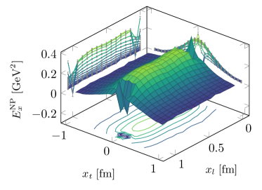
(a) $E_{x}^{NP}(x_{t},x_{l})$

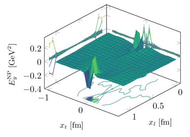
(b) $E_{y}^{NP}(x_{t},x_{l})$

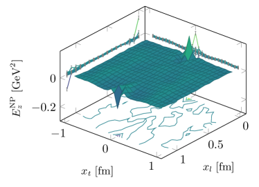
(c) $E_{z}^{NP}(x_{t},x_{l})$

Figure 4: Surface and contour plots for the three components of the nonperturbative chromoelectric field, $\vec{E}^{NP}\equiv\vec{E}-\vec{E}^{C}$, at $\beta=6.240$ and $d=1.142~{}$fm. All plotted quantities are in physical units.

Once $\vec{E}^{C}$ has been fixed, the difference Eq. (3) between the simulated field $\vec{E}$ and the field $\vec{E}^{C}$ determines $\vec{E}^{NP}$. In this way we obtain the nonperturbative structure of the flux tube. To the best of our knowledge, this is the first time that a confining part of the measured longitudinal chromoelectric field has been extracted making use only of lattice data.

In Fig. 4 we plot the longitudinal component $E_{x}^{NP}$ of the nonperturbative field (3) as a function of the longitudinal and transverse displacements $x_{l}$, $x_{t}$ at $\beta=6.240$. As expected, $E^{NP}$ is almost uniform along the flux tube at distances not too close to the static color sources. This feature is better seen in Fig. 6, where transverse sections of the field $E_{x}^{NP}(x_{l},x_{t})$, plotted in Fig. 4, are shown for the values of $x_{l}$ specified in Fig. 6. For these values of $x_{l}$ the shape of the nonperturbative longitudinal field is basically constant all along the axis.

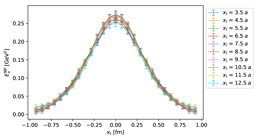
Figure 5: Transverse cross sections of the nonperturbative field $E_{x}^{NP}(x_{t})$ at $\beta=6.240$, $d=1.142$ fm, for several values of $x_{l}$.

Although figures 2,3, and 4 refer only to the case of $\beta=6.240$ and $d=1.142$ fm, the scenario is similar for the other two lattice setups listed in Table 1.

In Table 2 we also compare the values of the measured longitudinal chromoelectric field $E_{x}$ with those of the nonperturbative field $E_{x}^{NP}$ on the axis at the midpoint between the quark and antiquark, for all three values of their separation $d$. Given that $E^{NP}_{x}$ is almost uniform along the axis, $E_{x}^{NP}(x_{l},x_{t}=0)$ assumes these same values at all points $x_{l}$ on the axis for all distances larger than approximately $0.1-0.2~{}$fm from the quark sources.The value of $E_{x}^{NP}(x_{l},x_{t}=0)$ is closely related to the value of the string tension (see below). In future work we will use the distribution of color fields between a quark and an antiquark to calculate the force between them.

7 Future work

The value of the chromoelectric field at the position of the quarks is equal to force on the quarks Brambilla:2000gk , i.e. , the derivative of the heavy quark potential. However because the difficulty of carrying accurate simulations of the color field close to position of the source we cannot use our current simulations to determine the quark-antiquark force as a function of their separation. This is one goal of our future work.

We plan to compare the stress tensor density distribution calculated from our simulated color fields with the stress tensor density simulated in Ref. Yanagihara:2018qqg . This will provide a test of our vision of the space between static color charges as filled with lines of force of chromoelectric fields pointing in a color direction parallel to the color direction of the source, generating a Maxwell-like stress tensor in this color direction. Since there are fluctuations of the color fields in the other color directions, the width of the stress tensor density that we measure should be interpreted as the intrinsic width of the flux tube.

We can use our simulated stress tensor to calculate the force transmitted across the midplane and the resulting quark-antiquark force for the values of their separations where our simulations are carried out. These predictions can then be tested by comparing our simulated results with a parameterization of Wilson loop data for the long distance heavy quark potential. To the extent that the nonperturbative field $E^{NP}$ generates the long distance constant heavy quark force ( i.e., the string tension), and that the Coulomb-like field $E^{C}$ generates the $1/R^{2}$ correction to it, the force between a quark and an antiquark can be understood in terms of the color fields permeating the space between them.

8 Summary

In this paper we have determined the spatial distribution in three dimensions of all components of the color fields generated by a static quark-antiquark pair. We have found that the dominant component of the color field is the chromoelectric one in the longitudinal direction, i.e. in the direction along the axis connecting the two quark sources. This feature of the field distribution has been known for a long time. However, the accuracy of our numerical results allowed us to go far beyond this observation. First, we have found that all the chromomagnetic components of the color field are compatible with zero within the statistical uncertainties. Second, the chromoelectric components of the color fields in the directions transverse to the axis connecting the two sources, though strongly suppressed with respect to the longitudinal component, are sufficiently greater than the statistical uncertainties that we could manage to interpolate them.

Our remarkable finding was that the transverse components of the simulated chromoelectric field can be nicely reproduced by a Coulomb-like field generated by two sources with opposite charge (everywhere except in a small region around the sources). We then subtract this Coulomb-like field from the simulated chromoelectric field to obtain a nonperturbative field $\vec{E}^{NP}$ according to Eq. (3). The dependence of the resulting longitudinal component of $\vec{E}^{NP}$ on the distance $x_{t}$ from the axis is independent of the position $x_{l}$ along the axis, except near the sources. We identify the nonperturbative field found in this way from lattice simulations as the confining field of the QCD flux tube.

9 Discussion

We stress that our separation of the chromoelectric field into perturbative and nonperturbative components was obtained by directly analyzing lattice data on color field distributions between static quark sources. To the best of our knowledge this separation between perturbative and nonperturbative components has not been carried out previously.

The idea of this separation is independent of the procedure used in this paper to implement it. The separation provides a new tool with which to probe the chromoelectric field surrounding the quarks. Our approach can be straightforwardly extended to the case of QCD with dynamical fermions with physical masses and at nonzero temperature and baryon density.

Appendix A Smearing and renormalization

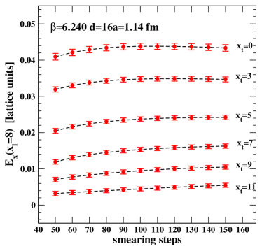
Figure 6: $E_{x}$ in lattice units versus smearing at $\beta=6.240$, $d=1.14$ fm, measured at the midpoint between sources ($x_{l}=8a$), for several values of $x_{t}$ (in lattice units).

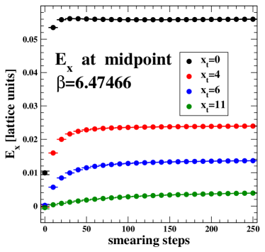
Figure 7: $E_{x}$ in lattice units at several values of $x_{t}$ versus smearing at $\beta=6.47466$ and $d=4a\simeq 0.37$ fm as in Ref. Battelli:2019lkz .

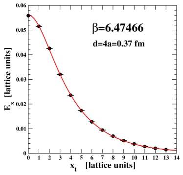
Figure 8: Clem fit (see Eq. 924) of Ref. Battelli:2019lkz to $E_{x}$ in lattice units at $\beta=6.47466$ and $d=4a\simeq 0.37$ fm. The values of $E_{x}$ have been measured after 100 smearing steps.

The typical behavior of the (unsubtracted) chromoelectric field in the longitudinal direction with our smearing setup is described in Fig. 6, which gives, at $\beta=6.240$ and for a distance $d=1.14$ fm between the sources, the field $E_{x}$ measured at the midpoint between sources ($x_{l}=8a$) for several values of the transverse distance $x_{t}$. We can clearly see that, for increasing number of the smearing steps, $E_{x}$ reaches a plateau for larger and larger values of $x_{t}$, with no sign whatsoever of degradation of the signal. The value of the smearing step quoted in the last column of Table 1 is such that all field components, on all transverse planes and at all values of $x_{t}$ (except possibly the few largest ones) have reached their plateaux.

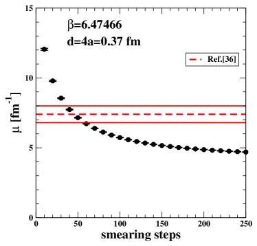
Figure 9: The Clem $\mu$ parameter (full black circles) versus smearing at $\beta=6.47466$ and $d=4a\simeq 0.37$ fm compared to the value obtained in Ref. Battelli:2019lkz (the red dashed line is the central value, the red full lines delimit the error band).

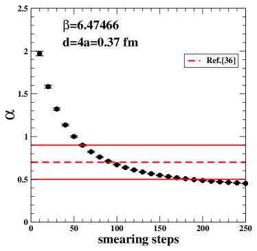
Figure 10: The Clem $\alpha$ parameter (full black circles) versus smearing at $\beta=6.47466$ and $d=4a\simeq 0.37$ fm compared to the value obtained in Ref. Battelli:2019lkz (the red dashed line is the central value, the red full lines delimit the error band).

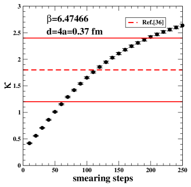
Figure 11: The Clem $\kappa$ parameter (full black circles) versus smearing at $\beta=6.47466$ and $d=4a\simeq 0.37$ fm compared to the value obtained in Ref. Battelli:2019lkz (the red dashed line is the central value, the red full lines delimit the error band).

Recently, a paper appeared Battelli:2019lkz which studied the flux tube between two static sources by means of a connected operator similar to ours, except that the role of the Wilson loop is replaced by two parallel and oppositely directed Polyakov loops. No smoothing is performed on the ensemble configuration, but the renormalization properties of the connected operator are properly taken into account. Their analysis of the (unsubtracted) longitudinal chromoelectric field at the midpoint between two sources separated by distance $d=4a\simeq 0.37$ fm gave the following values for the "Clem parameters” Clem:1975aa describing the transverse profile of the field:

$$\frac{1}{\lambda}=\mu=7.4(6)\ {\rm fm}^{-1}\;\;,\;\;\alpha=0.7(2)\ \;\;,\;\;\kappa=1.8(6)\,.$$ (5)

(See Eq.(24) of Ref. Battelli:2019lkz ).

To compare the analysis Ref. Battelli:2019lkz with our smearing procedure, we measured the longitudinal chromoelectric field $E_{x}$ at $\beta=6.47466$ and at a distance between the two static sources equal to $d=4a$. With the scale setting procedure used in Ref. Battelli:2019lkz this distance corresponds in physical units to the same quark-antiquark separation $d=0.37$ fm considered there. The behavior under smearing of the measured (unsubtracted) field $E_{x}$ at the midpoint between the sources and at different values of $x_{t}$ is shown in Fig. 7. The qualitative behavior is the same as in Fig. 6: the larger the number of smearing steps, the greater the number of values of $x_{t}$ for which $E_{x}$ has reached a plateau. We use the Clem parameterization to fit the transverse profiles. After 100 smearing steps, our determination of the parameters of the Clem fit gives

$$\frac{1}{\lambda}=\mu=5.73(2)\ {\rm fm}^{-1}\;,\;\;\alpha=0.67(1)\;,\;\;\kappa=1.65(2)\,,$$ (6)

The values of $\alpha$ and $\kappa$ are in nice agreement with Ref. Battelli:2019lkz but the difference in the values of $\mu$ requires further investigation. In Fig. 8 the fit is compared to data: it seems to be qualitatively very good, in spite of a $\chi^{2}/{\rm dof}$ of about $40$, probably due to the large correlation among data at different $x_{t}$, which were obtained in the same Monte Carlo simulation.

In Figs. 9, 10 and 11, we show the behavior of the parameters of the Clem fit versus smearing at $\beta=6.47466$ and $d=4a\simeq 0.37$ fm and compare them with the corresponding values as quoted in Ref. Battelli:2019lkz . The conclusion that can be drawn is that smearing behaves, not surprisingly, as an effective renormalization, driving the parameters towards the values extracted from the renormalized field. Of course, the different systematics in the two approaches must be carefully studied, to improve the matching.

Appendix B Coulomb fit

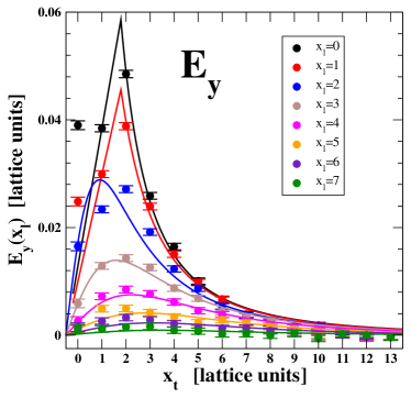
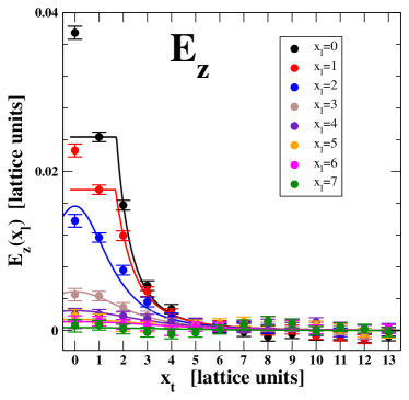
Figure 12: $E_{y}(x_{t})$ 12 and $E_{z}(x_{t})$ 12 and in lattice units at several values of $x_{l}$ at $\beta=6.240$, $d=16a\simeq 1.14$ fm, together with the Coulomb fit according to Eq. (4).

In this Appendix we give some details about the fit of the transverse components of the chromoelectric field with the Coulomb law given in Eq. (4). For definiteness, we concentrate on the case $\beta=6.240$ and distance between the sources equal to $d=16a\simeq 1.14$ fm. The other cases considered in this work were treated similarly.

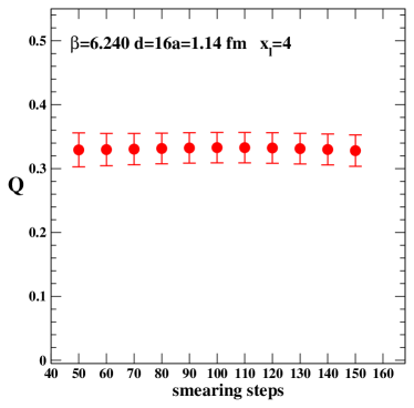
Figure 13: $Q$ from the Coulomb fit to $E_{y}$ field at $\beta=6.240$, $d=16a\simeq 1.14$ fm, and $x_{l}=4a$ versus smearing steps.

Table 3: Values of the fit parameters extracted from Coulomb fits of the $E_{y}$ field component at $\beta=6.240$ and $d=16a\simeq 1.14$ fm.

$x_{l}$	$Q$	$R_{0}$ [lattice units]	$\chi^{2}_{r}$
0	0.308(5)	2.287(24)	4.3
1	0.312(6)	2.498(32)	4.0
2	0.301(8)		14.3
3	0.333(15)		2.8
4	0.333(24)		2.6
5	0.313(37)		2.3
6	0.305(44)		1.6
7	0.269(86)		0.9

Table 4: Values of the fit parameters extracted from Coulomb fits of the $E_{z}$ field component at $\beta=6.240$ and $d=16a\simeq 1.14$ fm.

$x_{l}$	$Q$	$R_{0}$ [lattice units]	$\chi^{2}_{r}$
0	0.281(16)	1.792(41)	1.6
1	0.292(21)	2.018(60)	0.9
2	0.355(25)	2.422(65)	0.6
3	0.279(26)		0.2
4	0.341(54)		0.6
5	0.397(102)		1.1
6	0.626(191)		0.6
7	0.488(432)		0.9

In Fig. 12 we compare the profiles of the $y$- and $z$-components of the chromoelectric field on the transverse planes labeled by $x_{l}=0,\dots,7$ with fitting curves of the form given in (4). The field components were obtained after 100 smearing steps.

The fit parameters extracted from the Coulomb fit to $E_{y}$ and $E_{z}$ on transverse planes at $x_{l}\leq 7$ are summarized in Tables 3 and 4. For $x_{l}=0,1$ the point at $x_{t}=0$ has been excluded from the fit.

In order to obtain the final values for $Q$ (as well as for $R_{0}$), as quoted in Table 2, only Coulomb fits whose quality is higher than $10\%$, on datasets where the error on the largest extracted value of the field is $<20\%$, have been taken into account. Then weighted averages have been computed, along with the corresponding statistical error and a systematic uncertainty to account for the variability of $Q$ and $R_{0}$ among different acceptable fits.

The behavior of the $Q$ value so determined under smearing is shown in Fig. 13.

References

- (1) J. Greensite, An Introduction to the Confinement Problem, Lecture Notes in Physics (Springer Berlin Heidelberg, 2011), ISBN 9783642143816
- (2) D. Diakonov, Nucl. Phys. Proc. Suppl. 195, 5 (2009), 0906.2456
- (3) O. Philipsen, H. Wittig, Phys. Rev. Lett. 81, 4056 (1998), [Erratum: Phys. Rev. Lett. 83, 2684(1999)], hep-lat/9807020
- (4) S. Kratochvila, P. de Forcrand, Nucl. Phys. Proc. Suppl. 119, 670 (2003), hep-lat/0209094
- (5) G.S. Bali, H. Neff, T. Duessel, T. Lippert, K. Schilling (SESAM), Phys. Rev. D71, 114513 (2005), hep-lat/0505012
- (6) M. Fukugita, T. Niuya, Phys. Lett. B132, 374 (1983)
- (7) J.E. Kiskis, K. Sparks, Phys. Rev. D30, 1326 (1984)
- (8) J.W. Flower, S.W. Otto, Phys. Lett. B160, 128 (1985)
- (9) J. Wosiek, R.W. Haymaker, Phys. Rev. D36, 3297 (1987)
- (10) A. Di Giacomo, M. Maggiore, S. Olejnik, Phys. Lett. B236, 199 (1990)
- (11) A. Di Giacomo, M. Maggiore, S. Olejnik, Nucl. Phys. B347, 441 (1990)
- (12) P. Cea, L. Cosmai, Nucl. Phys. Proc. Suppl. 30, 572 (1993)
- (13) Y. Matsubara, S. Ejiri, T. Suzuki, Nucl. Phys. Proc. Suppl. 34, 176 (1994), hep-lat/9311061
- (14) P. Cea, L. Cosmai, Phys. Lett. B349, 343 (1995), hep-lat/9404017
- (15) P. Cea, L. Cosmai, Phys. Rev. D52, 5152 (1995), hep-lat/9504008
- (16) G.S. Bali, K. Schilling, C. Schlichter, Phys. Rev. D51, 5165 (1995), hep-lat/9409005
- (17) P. Skala, M. Faber, M. Zach, Nucl. Phys. B494, 293 (1997), hep-lat/9603009
- (18) R.W. Haymaker, T. Matsuki, Phys. Rev. D75, 014501 (2007), hep-lat/0505019
- (19) A. D’Alessandro, M. D’Elia, L. Tagliacozzo, Nucl. Phys. B774, 168 (2007), hep-lat/0607014
- (20) M.S. Cardaci, P. Cea, L. Cosmai, R. Falcone, A. Papa, Phys. Rev. D83, 014502 (2011), 1011.5803
- (21) P. Cea, L. Cosmai, A. Papa, Phys. Rev. D86, 054501 (2012), 1208.1362
- (22) P. Cea, L. Cosmai, F. Cuteri, A. Papa, PoS LATTICE2013, 468 (2013), 1310.8423
- (23) P. Cea, L. Cosmai, F. Cuteri, A. Papa, Phys. Rev. D89, 094505 (2014), 1404.1172
- (24) P. Cea, L. Cosmai, F. Cuteri, A. Papa, PoS LATTICE2014, 350 (2014), 1410.4394
- (25) N. Cardoso, M. Cardoso, P. Bicudo, Phys. Rev. D88, 054504 (2013), 1302.3633
- (26) M. Caselle, M. Panero, R. Pellegrini, D. Vadacchino, JHEP 01, 105 (2015), 1406.5127
- (27) P. Cea, L. Cosmai, F. Cuteri, A. Papa, Phys. Rev. D95, 114511 (2017), 1702.06437
- (28) E. Shuryak (2018), 1806.10487
- (29) M. Bander, Phys. Rept. 75, 205 (1981)
- (30) J. Greensite, Prog. Part. Nucl. Phys. 51, 1 (2003), hep-lat/0301023
- (31) G. Ripka, AIP Conf. Proc. 775, 262 (2005)
- (32) Y. A. Simonov, Phys. Rev. D99, 056012 (2019), 1804.08946
- (33) D.S. Kuzmenko, Y.A. Simonov, Phys. Lett. B494, 81 (2000), hep-ph/0006192
- (34) A. Di Giacomo, H.G. Dosch, V.I. Shevchenko, Y.A. Simonov, Phys. Rept. 372, 319 (2002), hep-ph/0007223
- (35) P. Cea, L. Cosmai, F. Cuteri, A. Papa, JHEP 06, 033 (2016), 1511.01783
- (36) N. Battelli, C. Bonati (2019), 1903.10463
- (37) R.G. Edwards, U.M. Heller, T.R. Klassen, Nucl. Phys. B517, 377 (1998), hep-lat/9711003
- (38) A. Hasenfratz, F. Knechtli, Phys. Rev. D64, 034504 (2001), hep-lat/0103029
- (39) M. Falcioni, M. Paciello, G. Parisi, B. Taglienti, Nuclear Physics B 251, 624 (1985)
- (40) M. Lüscher, Nucl. Phys. B180, 317 (1981)
- (41) S. Necco, R. Sommer, Nucl. Phys. B622, 328 (2002), hep-lat/0108008
- (42) O. Kaczmarek, F. Zantow, Phys. Rev. D71, 114510 (2005), hep-lat/0503017
- (43) F. Karbstein, M. Wagner, M. Weber, Phys. Rev. D98, 114506 (2018), 1804.10909
- (44) N. Brambilla, A. Pineda, J. Soto, A. Vairo, Phys. Rev. D63, 014023 (2001), hep-ph/0002250
- (45) R. Yanagihara, T. Iritani, M. Kitazawa, M. Asakawa, T. Hatsuda, Phys. Lett. B789, 210 (2019), 1803.05656
- (46) J.R. Clem, Journal of Low Temperature Physics 18, 427 (1975), 10.1007/BF00116134