Lagrangian Approximations for Stochastic Reachability of a Target Tube

Abstract

In this paper we examine how Lagrangian techniques can be used to compute underapproximations and overapproximation of the finite-time horizon, stochastic reach-avoid level sets for discrete-time, nonlinear systems. This approach is applicable for a generic nonlinear system without any convexity assumptions on the safe and target sets. We examine and apply our methods on the reachability of a target tube problem, a more generalized version of the finite-time horizon reach-avoid problem. Because these methods utilize a Lagrangian (set theoretic) approach, we eliminate the necessity to grid the state, input, and disturbance spaces allowing for increased scalability and faster computation. The methods scalability are currently limited by the computational requirements for performing the necessary set operations by current computational geometry tools. The primary trade-off for this improved extensibility is conservative approximations of actual stochastic reach set. We demonstrate these methods on several examples including the standard double-integrator, a chain of integrators, and a 4-dimensional space vehicle rendezvous docking problem.

1 Introduction

Reach-avoid analysis is an established verification tool that provides formal guarantees of both safety (by avoiding unsafe regions) and performance (by reaching a target set). Because of these guarantees, it is often used in systems that are safety-critical or expensive, such as space systems [1], avionics [2, 3], biomedical systems [4], and other applications [5, 6, 7]. The reach-avoid set is the set of states for which there exists a control that enables the state trajectory to reach a target at some finite time horizon, $N$, while remaining within a safe set (avoiding an unsafe set) for all instants in the time horizon. In a probabilistic system, satisfaction of the reach-avoid objective is accomplished stochastically. A dynamic programming-based solution characterizes the optimal value function, a function that assigns to each initial state the optimal probability of achieving the reach-avoid objective [8]. An appropriate level set of this value function provides the stochastic reach-avoid level set, the set of states for which probabilistic success of the reach-avoid objective is assured with at least the desired likelihood.

The theoretical framework for the probabilistic reach-avoid calculation uses dynamic programming [7, 8], and, hence, is computationally infeasible for even moderate-sized systems due to the gridding of not only the state-space, but also of the input and disturbance spaces [9]. Alternatives to dynamic programming include approximate dynamic programming [6, 10, 11], Gaussian mixtures [11], particle filters [1, 6], and convex chance-constrained optimization [1, 5]. These methods have been applied to systems that are at most 10-dimensional, at high memory and computational costs [6]. Further, since an analytical expression of the value function is not accessible, stochastic reach-avoid level sets can be computed only up to the accuracy of the gridding. Recently, a Fourier transform-based approach has provided greater scalability verifying LTI systems of dimension up to $40$ [12, 13]. In [13] the researchers established a set of sufficient conditions in which the stochastic reach-avoid set is convex and compact, enabling scalable polytopic underapproximation. However, this approach relies on numerical quadrature and is restricted to verifying the existence of open-loop controllers.

For deterministic systems (that is, systems without a disturbance input but with a control input) or systems with disturbances that come from a bounded set, Lagrangian methods for computing reachable sets are popular because they do not rely on a grid and can be computed efficiently for high-dimensional systems [4, 14, 15]. Rather than gridding the system, Lagrangian methods compute reachable sets through operations on sets, e.g. intersections, Minkowski summation, unions, etc. Thus, Lagrangian methods rely on computational geometry, whose scalability depends on the set representation and the computational difficulty of the operations used [14]. For example, sets that are represented as either vertex or facet polyhedra typically are limited by the need to solve the vertex-facet enumeration problem. Common set representations and relevant toolboxes for their implementation are: polyhedrons (MPT [16]), ellipsoids (ET [17]), zonotopes [18] (CORA [19]), star representation (HyLAA [20]), and support functions [21].

In this paper, we describe recursive techniques to obtain an under and an overapproximation of the probabilistic reach-avoid level set using Lagrangian methods. The underapproximation can be theoretically posed as the solution to the reachability of a target tube problem [22, 23, 24], originally framed to compute reachable sets of discrete-time controlled systems with bounded disturbance sets. Motivated by the scalability of the Lagrangian method proposed in [4, 25] for viability analysis in deterministic systems (that is, systems without a disturbance input but with a control input), we seek a similar approach to compute the underapproximation via tractable set theoretic operations. We originally demonstrated these methods in [26] unifying these approaches for the terminal-time reach-avoid problem. The reachability of a target tube problem is, however, a more generalized framework than the terminal-time reach-avoid problem. Hence, we extend [26] to the reachability of a target tube problem and additionally describe a recursive method for computing an overapproximation to the stochastic reach-avoid level set. Borrowing notation and terminology from [27] we call these under and overapproximations disturbance minimal and disturbance maximal reach sets, respectively.

The disturbance minimal reach set (underapproximation) is the set of initial states of the system for which there exists a disturbance that will remain in the target tube despite the worst case choice of a disturbance drawn from a bounded set $\operatorname{\mathcal{E}}$, i.e. for all disturbances in $\operatorname{\mathcal{E}}$. The disturbance maximal reach set (overapproximation) is the set of states for which there exists and input that will remain in the target tube given the best choice of a disturbance in a bounded set $\operatorname{\mathcal{O}}$, i.e. exists a disturbance in $\operatorname{\mathcal{O}}$. The original formulation [26] described the underapproximation for a single bounded disturbance set $\operatorname{\mathcal{E}}$. Here we will also demonstrate that we can use many different bounded disturbance sets $\operatorname{\mathcal{E}}_{i}$, $\operatorname{\mathcal{O}}_{i}$, $i\in\{1,\dots,M\}$, to help reduce the conservativeness of the approximations. Using multiple bounded disturbance sets requires repeated computations of the disturbance minimal and maximal reach sets. However, because of the reduced computational time from using Lagrangian methods we can use multiple disturbance sets and still provide substantially faster computation.

The remainder of the paper is as follows: Section 2 provides the necessary preliminaries and describes the problem formulation. In Section 3, we establish sufficient conditions for the bounded disturbance sets such that the disturbance minimal and maximal reach sets are a subset and superset of the stochastic reach set, respectively. Section 4 details the recursions for computing the disturbance minimal and disturbance maximal reach sets, given a single sufficient bounded disturbance set. Section 5 describes how these approximations can be improved by using multiple bounded disturbance sets. We examine numerical methods to obtain these sufficient bounded disturbance sets in Section 6 and examine the numerical implementation challenges for computing the disturbance minimal and maximal reach sets in Section 7. Finally, we demonstrate our algorithm on selected examples in Section 8 and provide conclusions and directions of future work in Section 9.

2 Preliminaries

The following notation will be used throughout the paper. We denote the set of natural numbers, including zero, as $\operatorname{\mathbb{N}}$, and discrete-time intervals with $\operatorname{\mathbb{N}}_{[a,b]}=\operatorname{\mathbb{N}}\cap\{a,a+1,\dots,b-1,b\}$, for $a,b\in\operatorname{\mathbb{N}}$, $a\leq b$. We will primarily use $k\in\operatorname{\mathbb{N}}$ as our discrete-time index but will also use $t\in\operatorname{\mathbb{N}}$ as necessary to provide clarity. The transposition of a vector is $x^{\top}$, and the concatenation of a discrete-time series of vectors is noted with a bar above the variable and a subscript with the indices, i.e. $\bar{x}_{[k,N]}=[x_{k}^{\top},x_{k+1}^{\top},\dots,x_{N}^{\top}]^{\top}$, $x_{t}\in\operatorname{\mathbb{R}}^{n}$ for $t\in\operatorname{\mathbb{N}}_{[k,N]}$. The $n$-dimensional identity matrix is noted as $I_{n}$.

The Minkowski summation of two sets $\mathcal{S}_{1},\mathcal{S}_{2}\subseteq\operatorname{\mathbb{R}}^{n}$ is $\mathcal{S}_{1}\oplus\mathcal{S}_{2}=\{s_{1}+s_{2}:s_{1}\in\mathcal{S}_{1},s_{2}\in\mathcal{S}_{2}\}$; the Minkowski difference (or Pontryagin difference) of two sets $\mathcal{S}_{1},\mathcal{S}_{2}$ is $\mathcal{S}_{2}\operatorname{\ominus}\mathcal{S}_{1}=\{s:s+s_{1}\in\mathcal{S}_{2}\ \forall s_{1}\in\mathcal{S}_{1}\}$. For $\operatorname{\mathcal{X}}\subseteq\operatorname{\mathbb{R}}^{n},n\in\mathbb{N},n>0$, the indicator function corresponding to a set $\mathcal{S}$ is $\boldsymbol{1}_{\mathcal{S}}:\operatorname{\mathcal{X}}\rightarrow\{0,1\}$ where $\boldsymbol{1}_{\mathcal{S}}(x)=1$ if $x\in\mathcal{S}$ and is zero otherwise; the Cartesian product of the set $\mathcal{S}$ with itself $k\in\mathbb{N}$ times is $\mathcal{S}^{k}$.

2.1 Lower semi-continuity

Lower semi-continuous (l.s.c.) functions are functions whose sub-level sets are closed [28, Definition 7.13]. Lower semi-continuous functions have very useful properties with respect to optimization.

• Indicator function of a closed set is l.s.c.: Given a closed set $S\subseteq\mathcal{X}$, the function $-\boldsymbol{1}_{S}(x)$ is l.s.c..

• Addition and l.s.c.: Given two l.s.c. functions $l_{1}(x),l_{2}(x):\mathcal{X}\rightarrow\operatorname{\mathbb{R}}$ such that $\forall x\in\mathcal{X}$, $|l_{1}(x)|\neq\infty$ and $|l_{2}(x)|\neq\infty$, the function $l_{1}(x)+l_{2}(x)$ is l.s.c. over $\mathcal{X}$ [29, Ex. 1.39].

• Semicontinuity under composition: Given a l.s.c. functions $l(x):\mathcal{X}\rightarrow\operatorname{\mathbb{R}}$ and a continuous function $C(x):\mathcal{Y}\rightarrow\mathcal{X}$, the function $l\circ C=l(C(\cdot)):\mathcal{Y}\rightarrow\operatorname{\mathbb{R}}$ is l.s.c. over $\mathcal{Y}\subseteq\operatorname{\mathbb{R}}^{m},\ m\in\mathbb{N},\ m>0$ [29, Ex. 1.40].

• Supremum of a l.s.c. function: Given $l:\mathcal{X}\times\mathcal{Y}\rightarrow\operatorname{\mathbb{R}}\cup\{-\infty,\infty\}$ such that $l$ is l.s.c., then $l^{\ast}(x)=\sup_{y\in\mathcal{Y}}l(x,y)=-\inf_{y\in\mathcal{Y}}(-l(x,y))$ is l.s.c. [28, Prop. 7.32(b)].

• Infimum of a l.s.c. function: Given $l:\mathcal{X}\times\mathcal{Y}\rightarrow\operatorname{\mathbb{R}}\cup\{-\infty,\infty\}$ such that $l$ is l.s.c. and $\mathcal{Z}\subseteq\mathcal{Y}$ is compact, then $l^{\ast}(x)=\inf_{y\in\mathcal{Z}}l(x,y)$ is l.s.c.. Additionally, there exists a Borel-measurable $\phi:\mathcal{X}\rightarrow\mathcal{Z}$ such that $l^{\ast}(x)=l(x,\phi(x)),\ \forall x\in\mathcal{X}$ [28, Prop. 7.33].

2.2 System description

Consider a discrete-time, nonlinear, time-varying dynamical system with an affine disturbance,

$$x_{k+1}=f_{k}(x_{k},u_{k})+w_{k}$$ (1)

with state $x_{k}\in\operatorname{\mathcal{X}}\subseteq\operatorname{\mathbb{R}}^{n}$, input $u_{k}\in\operatorname{\mathcal{U}}\subseteq\operatorname{\mathbb{R}}^{m}$, disturbance $w_{k}\in\operatorname{\mathcal{W}}\subseteq\operatorname{\mathbb{R}}^{n}$, and a function $f:\operatorname{\mathcal{X}}\times\operatorname{\mathcal{U}}\rightarrow\operatorname{\mathcal{X}}$. We denote the origin of $\operatorname{\mathbb{R}}^{n}$ as $0_{n}$ and assume $0_{n}\in\operatorname{\mathcal{W}}$ without loss of generality due to the affine nature of the disturbance. We also consider the discrete-time LTV system

$$x_{k+1}=A_{k}x_{k}+B_{k}u_{k}+w_{k}$$ (2)

with $A_{k}\in\operatorname{\mathbb{R}}^{n\times n}$ and $B_{k}\in\operatorname{\mathbb{R}}^{n\times m}$. We assume $A_{k}$ is non-singular, which holds true especially for discrete-time systems that arise from sampling continuous-time systems. We will consider the cases where $w_{k}$ is uncertain (non-stochastic disturbance drawn from a bounded set) and stochastic (random vector drawn from a known probability density function). The discrete horizon length for the reachability of a target tube problem is marked as $N\in\operatorname{\mathbb{N}}$, $N>0$.

2.3 Reachability of a target tube

As in [22, 30], we define a target tube $\mathscr{T}_{N}=[\operatorname{\mathcal{T}}_{0},\operatorname{\mathcal{T}}_{1},\dots,\operatorname{\mathcal{T}}_{N}]$, as an indexed collection of subsets of the state space, $\operatorname{\mathcal{T}}_{k}\subseteq\operatorname{\mathcal{X}}$, for all $k\in\operatorname{\mathbb{N}}_{[0,N]}$. We assign attributes of the tube that are typically given to sets, e.g. closed, bounded, compact, convex, etc., if and only if every set in the target tube has those properties. For example, we say that the target tube $\operatorname{\mathscr{T}}_{N}$ is closed if and only if $\operatorname{\mathcal{T}}_{k}$ is closed for all $k\in\operatorname{\mathbb{N}}_{[0,N]}$.

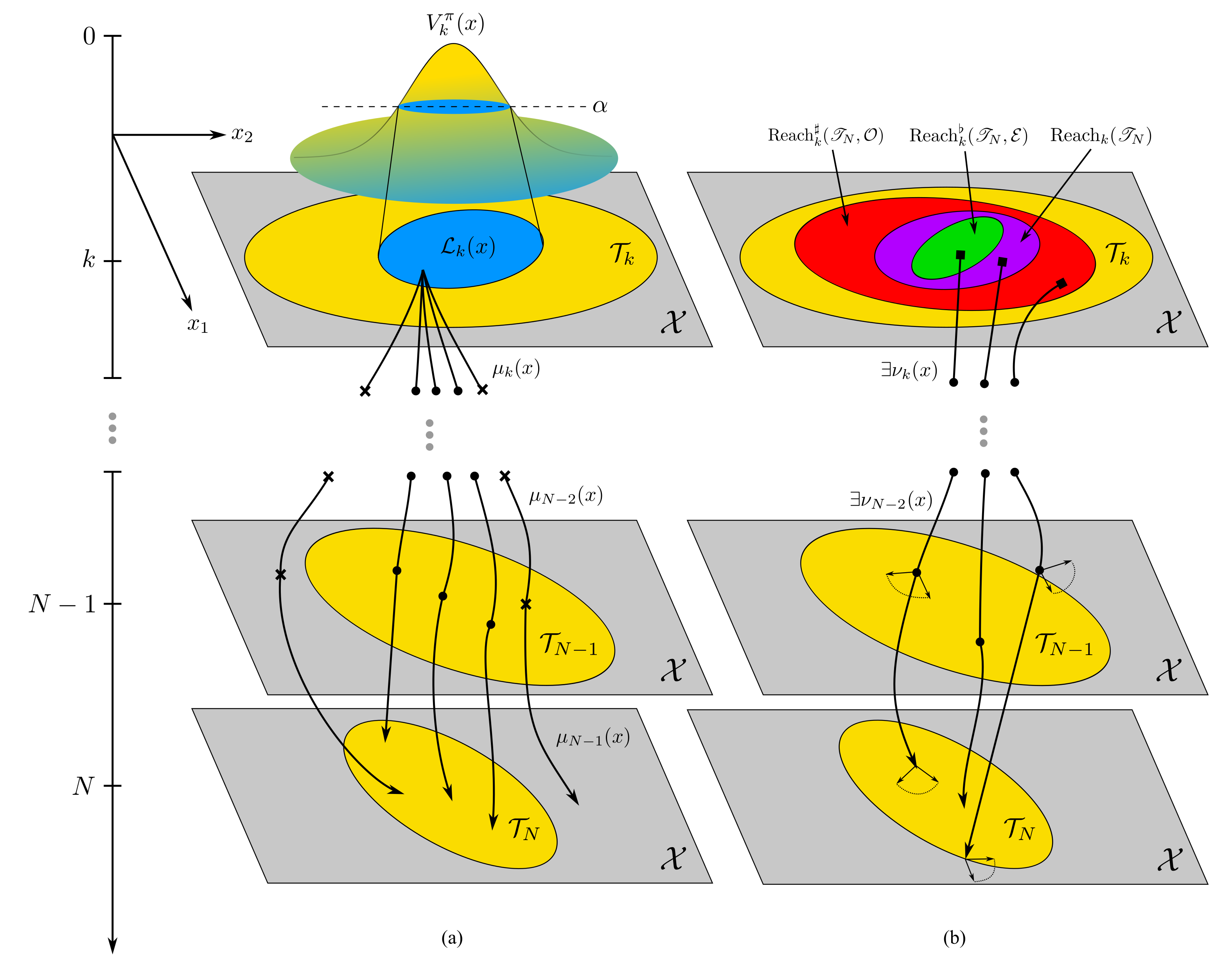
Figure 1: Graphical representation of (a) the stochastic $\alpha$-level reach set, $\mathcal{L}_{k}(\operatorname{\mathscr{T}}_{N},\alpha)$ and (b) of the reachability of the target tube—$\operatorname{Reach}_{k}(\operatorname{\mathscr{T}}_{N})$, (3), the disturbance minimal reach set—$\operatorname{Reach}_{k}^{\flat}(\operatorname{\mathscr{T}}_{N},\operatorname{\mathcal{E}})$, (7), and the disturbance maximal reach set—$\operatorname{Reach}_{k}^{\sharp}(\operatorname{\mathscr{T}}_{N},\operatorname{\mathcal{O}})$, (8). The trajectories with circle markings (•) remain in the target tube while trajectories with an ex (x) fail to remain in the tube. For the stochastic reach set starting from the same initial condition, some trajectories will not remain in the target tube due to the random nature of the disturbance. For the disturbance minimal and maximal reach reach set the trajectories need to remain in the target set for all disturbances in $\operatorname{\mathcal{E}}$, and some disturbance in $\operatorname{\mathcal{O}}$, respectively. The reachability of a target tube set, $\operatorname{Reach}_{k}(\operatorname{\mathscr{T}}_{N})$, does not consider a disturbance and, hence, has a deterministic trajectory.

We will denote an admissible state-feedback law using $\nu:\operatorname{\mathcal{X}}\rightarrow\operatorname{\mathcal{U}}$, the set of admissible state-feedback laws with $\mathcal{F}$, and the set of admissible control policies $\rho=[\nu_{0}(\cdot),\nu_{1}(\cdot),\dots,\nu_{N-1}(\cdot)]$ using $\mathcal{P}=\mathcal{F}^{N}$.

The reachability of a target tube problem is concerned with determining the set of states at time $k\in\operatorname{\mathbb{N}}$ for which there exists a control policy, $\rho$, such that, for the system (1) with no disturbance, i.e. $\mathcal{W}=\{0_{n}\}$, the trajectory $[x_{k},\dots,x_{N}]$ will remain in the target tube. Formally,

$$\operatorname{Reach}_{k}(\operatorname{\mathscr{T}}_{N})=\big{\{}x_{k}\in\operatorname{\mathcal{T}}_{k}:\; \forall t\in\operatorname{\mathbb{N}}_{[k,N-1]},\exists\nu_{t}\in\mathcal{F},$$

$$x_{t+1}\in\operatorname{\mathcal{T}}_{t+1}\big{\}}$$ (3)

This set can be seen graphically in Figure LABEL:fig:uncertain-reach-sets.

The motivation for using target tubes is to allow for more versatility in the problem definition. We can unite the standard terminal-time reach-avoid problem—in which we desire to reach a target, $\operatorname{\mathcal{T}}$, at time $N$ while remaining in a safe set, $\operatorname{\mathcal{K}}$, for $k<N$—and the reachability of target tubes with $\operatorname{\mathscr{T}}_{N}^{RA}=[\operatorname{\mathcal{K}},\operatorname{\mathcal{K}},\dots,\operatorname{\mathcal{K}},\operatorname{\mathcal{T}}]$. The viability problem can equivalently be subsumed with $\operatorname{\mathscr{T}}_{N}^{V}=[\operatorname{\mathcal{K}},\operatorname{\mathcal{K}},\dots,\operatorname{\mathcal{K}}]$. However many interesting problems fit outside of the standard terminal-time reach-avoid or viability problems.

2.4 Stochastic reachability of a target tube

The basic reachability of a target tube problem (3) is described with no disturbance. Here we consider (1), with a stochastic disturbance $w_{k}$. We assume $w_{k}$ is an $n$-dimensional random vector defined in the probability space $(\operatorname{\mathcal{W}},\sigma(\operatorname{\mathcal{W}}),\mathbb{P}_{w})$; $\sigma(\operatorname{\mathcal{W}})$ denotes the minimal $\sigma$-algebra associated with the random vector $w_{k}$. We assume the disturbance $w_{k}$ is absolutely continuous with a probability density function $\psi_{w}$ and the disturbance process ${\{w_{k}\}}_{k=0}^{N-1}$ is an independent and identically distributed (i.i.d.) random process.

We will denote an admissible universally-measurable state-feedback law as $\mu:\operatorname{\mathcal{X}}\rightarrow\operatorname{\mathcal{U}}$ and the set of Markov control policies $\pi=[\mu_{0}(\cdot),\mu_{1}(\cdot),\dots,\mu_{N-1}(\cdot)]$ as $\mathcal{M}$. Since no measurability restrictions were imposed on the admissible feedback laws in Section 2.3, $\mathcal{M}\subset\mathcal{P}$. Given a Markov policy $\pi$ and initial state $x_{0}\in\operatorname{\mathcal{X}}$, the concatenated state vector $\bar{x}_{[1,N]}=[x_{1}^{\top},\dots,x_{N}^{\top}]^{\top}$ for the system (1) is a random vector defined in the probability space $(\operatorname{\mathcal{X}}^{N},\sigma(\operatorname{\mathcal{X}}^{N}),\operatorname{\mathbb{P}}_{\bar{x}_{[1,N]}}^{x_{0},\pi})$. The probability measure $\operatorname{\mathbb{P}}_{\bar{x}_{[1,N]}}^{x_{0},\pi}$ is induced from the sequence of random variables $\bar{w}_{[0,N-1]}$ defined on the probability space $(\operatorname{\mathcal{W}}^{N},\sigma(\operatorname{\mathcal{W}}^{N}),\operatorname{\mathbb{P}}_{\bar{w}_{[0,N-1]}})$, as seen in [7, Sec. 2]. For $k\in\mathbb{N}_{[0,N-1]}$, we denote the probability space associated with the random vector $\bar{x}_{[k+1,N]}$ as $(\operatorname{\mathcal{X}}^{N-k},\sigma(\operatorname{\mathcal{X}}^{N-k}),\operatorname{\mathbb{P}}_{\bar{x}_{[k+1,N]}}^{x_{k},\pi})$.

For stochastic reachability analysis, we are interested in the maximum likelihood that the system (1) starting at an initial state $x_{0}\in\operatorname{\mathcal{X}}$ will stay within the target tube using a Markov policy. The maximum likelihood and the optimal Markov policy can be determined as the solution to the optimization problem, [7, Sec. 4]

$$\sup_{\pi\in\mathcal{M}}\mathbb{E}^{N,\pi}_{\bar{x}}\left[\prod_{i=0}^{N}\boldsymbol{1}_{\operatorname{\mathcal{T}}_{i}}(x_{i})\right].$$ (4)

Let the optimal solution to problem (4) be $\pi^{\ast}=[\mu_{0}^{\ast}(\cdot)\ \ldots\ \mu_{N-1}^{\ast}(\cdot)]$, the maximal Markov policy in the terminal sense [7, Def. 10]. A dynamic programming approach was presented in [7] to solve problem (4), along with sufficient conditions for the existence of a maximal Markov policy. This approach computes value functions $V_{k}^{\ast}:\operatorname{\mathcal{X}}\rightarrow[0,1]$ for $k\in[0,N]$,

$$V_{N}^{\ast}(x) =\boldsymbol{1}_{\mathcal{T}_{N}}(x)$$ (5a)

$$V_{k}^{\ast}(x) =\boldsymbol{1}_{\operatorname{\mathcal{T}}_{k}}(x)\int_{\operatorname{\mathcal{X}}}V_{k+1}^{\ast}(y)Q(dy|x,u)$$

$$=\boldsymbol{1}_{\operatorname{\mathcal{T}}_{k}}(x)\operatorname{\mathbb{P}}_{\bar{x}_{[k+1,N]}}^{x_{k},\pi^{\ast}}\left(\bigcap_{t=k+1}^{N}\{x_{t}\in\operatorname{\mathcal{T}}_{t}\}\Big{|}x_{k}=x\right)$$ (5b)

where $Q(\cdot|x,u)$ is the one-step transition kernel [7]. For notational convenience we will often simplify the $x_{k}=x$ condition in probability statements and simply write $\operatorname{\mathbb{P}}_{\bar{x}_{[k+1,N]}}^{x_{k},\pi^{\ast}}\left(\cdot|x_{k}=x\right)$ as $\operatorname{\mathbb{P}}_{\bar{x}_{[k+1,N]}}^{x_{k},\pi^{\ast}}\left(\cdot|x\right)$.

$$V_{k}^{\ast}(x) =\operatorname{\mathbb{P}}_{\bar{x}_{[k+1,N]}}^{x_{k},\pi^{\ast}}\Bigg{(}\bigcap_{t=k+1}^{N}\{x_{t}\in\operatorname{\mathcal{T}}_{t}\}\Big{|}x\Bigg{)}\boldsymbol{1}_{\operatorname{\mathcal{T}}_{k}}(x)$$

$$=\operatorname{\mathbb{P}}_{\bar{x}_{[k+1,N]}}^{x_{k},\pi^{\ast}}\Bigg{(}\bigcap_{t=k+1}^{N}\{x_{t}\in\operatorname{\mathcal{T}}_{t}\}\Big{|}x,\bar{w}_{[k,N-1]}\in\operatorname{\mathcal{E}}^{N-k}\Bigg{)}\operatorname{\mathbb{P}}_{\bar{w}_{[k,N-1]}}(\bar{w}_{[k,N-1]}\in\operatorname{\mathcal{E}}^{N-k})$$

$$\qquad+\operatorname{\mathbb{P}}_{\bar{x}_{[k+1,N]}}^{x_{k},\pi^{\ast}}\Bigg{(}\bigcap_{t=k+1}^{N}\{x_{t}\in\operatorname{\mathcal{T}}_{t}\}\Big{|}x,\bar{w}_{[k,N-1]}\in(\mathcal{W}^{N-k}\setminus\operatorname{\mathcal{E}}^{N-k})\Bigg{)}\operatorname{\mathbb{P}}_{\bar{w}_{[k,N-1]}}(\bar{w}_{[k,N-1]}\in(\mathcal{W}^{N-k}\setminus\operatorname{\mathcal{E}}^{N-k}))$$ (10)

$$\geq\operatorname{\mathbb{P}}_{\bar{x}_{[k+1,N]}}^{x_{k},\pi^{\ast}}\Bigg{(}\bigcap_{t=k+1}^{N}\{x_{t}\in\operatorname{\mathcal{T}}_{t}\}\Big{|}x,\bar{w}_{[k,N-1]}\in\operatorname{\mathcal{E}}^{N-k}\Bigg{)}\operatorname{\mathbb{P}}_{\bar{w}_{[k,N-1]}}(\bar{w}_{[k,N-1]}\in\operatorname{\mathcal{E}}^{N-k}).$$ (11)

By definition, the optimal value function $V_{0}^{\ast}(x_{0})$ provides the maximum likelihood of ensuring that the system (1) stays within the target tube $\operatorname{\mathscr{T}}_{N}$ when initialized to the initial state $x_{0}\in\operatorname{\mathcal{X}}$. Note that the problem discussed in [7] was specifically a reach-avoid problem, but it may be easily extended to the more general case discussed here yielding the recursion (5).

For $\alpha\in[0,1]$ and $k\in\mathbb{N}_{[0,N]}$, the stochastic $\alpha$-level reach set,

$$\mathcal{L}_{k}(\operatorname{\mathscr{T}}_{N},\alpha) =\Bigg{\{}y\in\operatorname{\mathcal{T}}_{k}:$$

$$\hskip-28.45274pt\sup_{\pi\in\mathcal{M}}\operatorname{\mathbb{P}}_{\bar{x}_{[k+1,N]}}^{x_{k},\pi}\Bigg{(}\bigcap_{t=k+1}^{N}\{\bar{x}_{t}\in\operatorname{\mathcal{T}}_{t}\}\;\Big{|}\;y\Bigg{)}\geq\alpha\Bigg{\}},$$

$$=\left\{y\in\operatorname{\mathcal{T}}_{k}:V_{k}^{\ast}(x)\geq\alpha\right\}$$ (6)

is the set of states $x$ that achieve the reachability of a target tube objective with a minimum probability $\alpha$. This set is shown graphically in Figure LABEL:fig:stoch-reach-set. For brevity we will often refer to the stochastic $\alpha$-level reach set simply as the stochastic reach set.

2.5 Disturbance minimal and maximal reachability of a target tube

Now, consider the nonlinear system, (1), with an uncertain disturbance $w_{k}$ drawn from a bounded disturbance set. Two types of phenomena are of interest: the disturbance minimal reachability of a target tube and the disturbance maximal reachability of a target tube. In this subsection, we will treat the disturbance as a non-stochastic uncertainty. For these problems we also consider admissible state-feedback policies, $\rho\in\mathcal{P}$.

For the disturbance minimal reachability problem, we are interested in the existence of a feedback controller $\rho\in\mathcal{P}$ for which the system (1) will remain in a target tube, $\operatorname{\mathscr{T}}_{N}$, despite the worst possible choice of the disturbance $w_{k}\in\operatorname{\mathcal{E}}$. The set of states $x_{k}$ for $k\in\mathbb{N}_{[0,N-1]}$ which may be driven by such a control policy is the $k$-time disturbance minimal reach set

$$\operatorname{Reach}_{k}^{\flat}(\operatorname{\mathscr{T}}_{N},\operatorname{\mathcal{E}})=\big{\{}x_{k}\in\operatorname{\mathcal{T}}_{k}:\; \forall t\in\operatorname{\mathbb{N}}_{[k,N-1]},\exists\nu_{t}\in\mathcal{F},$$

$$\forall w_{t}\in\operatorname{\mathcal{E}},x_{t+1}\in\operatorname{\mathcal{T}}_{t+1}\big{\}}$$ (7)

The problem of disturbance maximal reachability of the target tube concerns the system (1) with $w_{k}\in\operatorname{\mathcal{O}}\subseteq\mathcal{W}$. Here, we seek a feedback controller $\rho\in\mathcal{P}$ ensures that the system stays within the target tube, under the best possible choice for the disturbance $w_{k}\in\mathcal{O}$. The set of states $x_{k}$ for $k\in\mathbb{N}_{[0,N-1]}$ which may be driven by such a control policy is the $k$-time disturbance maximal reach set,

$$\operatorname{Reach}_{k}^{\sharp}(\operatorname{\mathscr{T}}_{N},\operatorname{\mathcal{O}})=\big{\{}x_{k}\in\operatorname{\mathcal{T}}_{k}:\; \forall t\in\operatorname{\mathbb{N}}_{[k,N-1]},\exists\nu_{t}\in\mathcal{F},$$

$$\exists w_{t}\in\operatorname{\mathcal{O}},x_{t+1}\in\operatorname{\mathcal{T}}_{t+1}\big{\}}.$$ (8)

The disturbance minimal and maximal reach sets, (7) and (8), can be seen graphically in Figure LABEL:fig:uncertain-reach-sets.

For brevity, when the discrete-time index $k$ is apparent, we will refer to the $k$-time disturbance minimal and maximal reach sets more succinctly as the disturbance minimal and disturbance maximal reach sets. Note that the disturbance minimal reach set is equivalent to the well studied in reachability of target tube problem [22, 30], and is also known as the robust controllable set in model predictive control community [15].

2.6 Problem statements

This paper utilizes disturbance minimal and maximal reach sets to efficiently and scalably approximate the stochastic $\alpha$-level reach set. We achieve this by addressing the following problems:

Problem 1.

Given a value $\alpha\in[0,1]$, characterize $\operatorname{\mathcal{E}},\operatorname{\mathcal{O}}\subseteq\operatorname{\mathcal{W}}$ whose corresponding disturbance minimal and maximal reach sets respectively under and overapproximate the stochastic effective $\alpha$-level set (6), i.e., find $\operatorname{\mathcal{E}},\operatorname{\mathcal{O}}\subseteq\operatorname{\mathcal{W}}$ such that $\operatorname{Reach}_{0}^{\flat}(\operatorname{\mathscr{T}}_{N},\operatorname{\mathcal{E}})\subseteq\mathcal{L}_{0}(\operatorname{\mathscr{T}}_{N},\alpha)\subseteq\operatorname{Reach}_{0}^{\sharp}(\operatorname{\mathscr{T}}_{N},\operatorname{\mathcal{O}})$.

Problem 1.a.

Characterize the sufficient conditions for which the optimal control policy corresponding to the disturbance minimal and maximal reach sets is a Markov control policy for the system (1).

Next, we discuss convex optimization-based techniques to construct $\operatorname{\mathcal{E}}$ and $\operatorname{\mathcal{O}}$.

Problem 2.

Propose computationally efficient methods to compute $\operatorname{\mathcal{E}},\operatorname{\mathcal{O}}\subseteq\mathcal{W}$ that satisfy Problem 1.

We will also discuss the min-max and min-min problems that may be used to obtain these sets [30, Sec. 4.6.2].

Problem 3.

Construct Lagrangian-based recursions for the exact computation of the $k$-time disturbance minimal and disturbance maximal reach sets for the system (1).

Problem 4.

Improve the approximations obtained via Problem 1 by using multiple disturbance subsets.

3 Lagrangian approximations for the stochastic effective level sets

In this section we will details how disturbance minimal and maximal reach sets are used to approximate stochastic reach sets. We will first detail the conditions upon $\operatorname{\mathcal{E}}$ which allow for the disturbance minimal reach set to be a conservative underapproximation, and then will detail the conditions for $\operatorname{\mathcal{O}}$ that ensures that the disturbance maximal reach set will provide an overapproximation. The theory in this section will require the conditions stated in the following assumption.

Assumption 1.

The target tube $\operatorname{\mathscr{T}}_{N}$ is closed, the input space $\operatorname{\mathcal{U}}$ is compact, and $f$ is continuous in $\operatorname{\mathcal{X}}\times\operatorname{\mathcal{U}}$.

3.1 Underapproximation of the stochastic $\alpha$-level reach set

We will first address Problem 1.a via Theorem 1.

Theorem 1.

Under Assumption 1, there exists an optimal Markov policy $\pi^{\ast}\in\mathcal{M}\subset\mathcal{P}$ associated with the set $\operatorname{Reach}_{0}^{\flat}(\operatorname{\mathscr{T}}_{N},\operatorname{\mathcal{E}})$.

The proof for Theorem 1 is deferred to Section 4.4. The guarantee of the existence of an optimal Markov policy for the robust effective target set allows for the definition of the probability measure $\operatorname{\mathbb{P}}_{\bar{x}_{[k+1,N]}}^{x_{k},\pi}(\cdot|y)$, which is essential for demonstrating the conditions upon $\operatorname{\mathcal{E}}$ that will make the disturbance minimal reach set a conservative approximation of the stochastic reach set, as will be shown in the following Proposition and Theorem.

Proposition 1.

Under Assumption 1, for every $k\in\operatorname{\mathbb{N}}_{[0,N-1]}$, if $y\in\operatorname{Reach}_{k}^{\flat}(\operatorname{\mathscr{T}}_{N},\operatorname{\mathcal{E}})$, then

$$\operatorname{\mathbb{P}}_{\bar{x}_{[k+1,N]}}^{x_{k},\pi^{\ast}}\Bigg{(}\bigcap_{t=k+1}^{N}\{x_{t}\in\operatorname{\mathcal{T}}_{t}\}\;\Big{|}\; y,\bar{w}_{[k,N-1]}\in\operatorname{\mathcal{E}}^{N-k}\Bigg{)}=1.$$ (9)

Proof: Theorem 1 ensures that the probability measure on the left-hand side of (9) exists. The equality is thus ensured by the definition of the disturbance minimal reach set, (7).   

Theorem 2.

Under Assumption 1, for some $\alpha\in[0,1]$, $k\in\operatorname{\mathbb{N}}_{[0,N-1]}$, and $\operatorname{\mathcal{E}}\subseteq\mathcal{W}$ such that for all $t\in\operatorname{\mathbb{N}}_{[k,N-1]}$, $\mathbb{P}_{w}(w_{t}\in\operatorname{\mathcal{E}})={\alpha}^{\frac{1}{N-k}}$, then $\operatorname{Reach}_{k}^{\flat}(\operatorname{\mathscr{T}}_{N},\operatorname{\mathcal{E}})\subseteq\mathcal{L}_{k}(\alpha)$.

Proof: We are interested in underapproximating $\mathcal{L}_{k}(\operatorname{\mathscr{T}}_{N},\alpha)$ as defined in (6). If $x\in\operatorname{Reach}_{k}^{\flat}(\operatorname{\mathscr{T}}_{N},\operatorname{\mathcal{E}})$, then Equation 10 follows from (5b) by Theorem 1, the law of total probability, and the definition of the robust effective target set (7)—which implies that $\boldsymbol{1}_{\operatorname{\mathcal{T}}_{k}}(x)=1$. Equation (11) follows from (10) after ignoring the second term (which is non-negative). Simplifying (11) using Proposition 1 and the i.i.d. assumption of the disturbance process, we obtain

$$V_{k}^{\ast}(x) \geq\operatorname{\mathbb{P}}_{\bar{w}_{[k,N-1]}}(\bar{w}_{[k,N-1]}\in\operatorname{\mathcal{E}}^{N-k})$$

$$=\left(\mathbb{P}_{w}(w_{t}\in\operatorname{\mathcal{E}})\right)^{N-k}=\alpha.$$ (12)

Thus, if $x\in\operatorname{Reach}_{k}^{\flat}(\operatorname{\mathscr{T}}_{N},\operatorname{\mathcal{E}})$ then $x\in\mathcal{L}_{k}(\operatorname{\mathscr{T}}_{N},\alpha)$ by (6), implying $\operatorname{Reach}_{k}^{\flat}(\operatorname{\mathscr{T}}_{N},\operatorname{\mathcal{E}})\subseteq\mathcal{L}_{k}(\operatorname{\mathscr{T}}_{N},\alpha)$.   

Theorem 2 characterizes conditions upon $\operatorname{\mathcal{E}}$ such that $\operatorname{Reach}_{k}^{\flat}(\operatorname{\mathscr{T}}_{N},\operatorname{\mathcal{E}})$ will be a conservative underapproximation of $\mathcal{L}_{k}(\operatorname{\mathscr{T}}_{N},\alpha)$. This will allow for fast underapproximations of $\mathcal{L}_{k}(\operatorname{\mathscr{T}}_{N},\alpha)$ to be determined through Lagrangian computation of the robust effective target set. These methods will be further detailed in Section 4.

$$\operatorname{\mathbb{P}}_{\bar{x}_{[k+1,N]}}^{x_{k},\pi}\left(\bigcup_{t=k+1}^{N}\{x_{t}\not\in\operatorname{\mathcal{T}}_{t}\}\Big{|}y\right) =\operatorname{\mathbb{P}}_{\bar{x}_{[k+1,N]}}^{x_{k},\pi}\left(\bigcup_{t=k+1}^{N}\{x_{t}\not\in\operatorname{\mathcal{T}}_{t}\}\Big{|}y,\bar{w}_{[k,N-1]}\in\operatorname{\mathcal{O}}^{N-k}\right)\operatorname{\mathbb{P}}_{\bar{w}_{[k,N-1]}}(\bar{w}_{[k,N-1]}\in\operatorname{\mathcal{O}}^{N-k})$$

$$\hskip 28.45274pt+\operatorname{\mathbb{P}}_{\bar{x}_{[k+1,N]}}^{x_{k},\pi}\left(\bigcup_{t=k+1}^{N}\{x_{t}\not\in\operatorname{\mathcal{T}}_{t}\}\Big{|}y,\bar{w}_{[k,N-1]}\not\in\operatorname{\mathcal{O}}^{N-k}\right)\operatorname{\mathbb{P}}_{\bar{w}_{[k,N-1]}}(\bar{w}_{[k,N-1]}\not\in\operatorname{\mathcal{O}}^{N-k})$$

$$\geq\operatorname{\mathbb{P}}_{\bar{x}_{[k+1,N]}}^{x_{k},\pi}\left(\bigcup_{t=k+1}^{N}\{x_{t}\not\in\operatorname{\mathcal{T}}_{t}\}\Big{|}y,\bar{w}_{[k,N-1]}\in\operatorname{\mathcal{O}}^{N-k}\right)\operatorname{\mathbb{P}}_{\bar{w}_{[k,N-1]}}(\bar{w}_{[k,N-1]}\in\operatorname{\mathcal{O}}^{N-k}).$$ (15)

3.2 Overapproximation of the stochastic $\alpha$-level reach set

We now move to the less common analysis of the overapproximation of the stochastic $\alpha$-level reach set.

Theorem 3.

Under Assumption 1, $\alpha\in[0,1]$, some $k\in\operatorname{\mathbb{N}}_{[0,N]}$, and $\operatorname{\mathcal{O}}\subseteq\mathcal{W}$ such that for all $t\in\operatorname{\mathbb{N}}_{[0,N-1]}$, $\mathbb{P}_{w}(w_{t}\in\operatorname{\mathcal{O}})={(1-\alpha)}^{\frac{1}{N-k}}$, then $\operatorname{Reach}_{k}^{\sharp}(\operatorname{\mathscr{T}}_{N},\operatorname{\mathcal{O}})\subseteq\mathcal{L}_{k}(\alpha)$.

Proof: After characterizing $\operatorname{\mathcal{X}}\setminus\mathcal{L}_{k}(\operatorname{\mathscr{T}}_{N},\alpha)$ and $\operatorname{\mathcal{X}}\setminus\operatorname{Reach}_{k}^{\sharp}(\operatorname{\mathscr{T}}_{N},\operatorname{\mathcal{O}})$, we will show that, $y\in\operatorname{\mathcal{X}}\setminus\operatorname{Reach}_{k}^{\sharp}(\operatorname{\mathscr{T}}_{N},\operatorname{\mathcal{O}})\Rightarrow y\in\operatorname{\mathcal{X}}\setminus\mathcal{L}_{k}(\alpha)$, for the given $\operatorname{\mathcal{O}}$. This implies that $\operatorname{\mathcal{X}}\setminus\operatorname{Reach}_{k}^{\sharp}(\operatorname{\mathscr{T}}_{N},\operatorname{\mathcal{O}})\subseteq\operatorname{\mathcal{X}}\setminus\mathcal{L}_{k}(\alpha)\Rightarrow\mathcal{L}_{k}(\alpha)\subseteq\operatorname{Reach}_{k}^{\sharp}(\operatorname{\mathscr{T}}_{N},\operatorname{\mathcal{O}})$, as desired.

Using DeMorgan’s law, we can write $\operatorname{\mathcal{X}}\setminus\mathcal{L}_{k}(\operatorname{\mathscr{T}}_{N},\alpha)$ as in Equation 17. From the definition of (8),

$$\operatorname{\mathcal{X}}\setminus\operatorname{Reach}_{k}^{\sharp}(\operatorname{\mathscr{T}}_{N},\operatorname{\mathcal{O}}) =\big{\{}x_{k}\in\operatorname{\mathcal{X}}:\exists t\in\operatorname{\mathbb{N}}_{[k,N-1]},\forall\nu_{t}\in\mathcal{F},$$

$$\hskip 59.75095pt\forall w_{t}\in\operatorname{\mathcal{O}},x_{t+1}\not\in\operatorname{\mathcal{T}}_{t+1}\big{\}}.$$ (13)

Hence, given $y\in\operatorname{\mathcal{X}}\setminus\operatorname{Reach}_{k}^{\sharp}(\operatorname{\mathscr{T}}_{N},\operatorname{\mathcal{O}})$, for any admissible control policies ($\rho\in\mathcal{P}$), and specifically any Markov control policies ($\pi\in\mathcal{M}$) since $\mathcal{M}\subset\mathcal{P}$,

$$\operatorname{\mathbb{P}}_{\bar{x}_{[k+1,N]}}^{x_{k},\pi}\Bigg{(}\bigcup_{t=k+1}^{N}\{\bar{x}_{t}\not\in\operatorname{\mathcal{T}}_{t}\}\;\Big{|}\; y,\bar{w}_{[k,N-1]}\in\operatorname{\mathcal{O}}^{N-k}\Bigg{)}=1$$ (14)

By the law of total probability, we have (15). Since $\mathbb{P}_{w}(w_{t}\in\operatorname{\mathcal{O}})=(1-\alpha)^{\frac{1}{N-k}},\ \forall t\in\mathbb{N}_{[k,N-1]}$, and the disturbance $w_{t}$ is i.i.d.,

$$\operatorname{\mathbb{P}}_{\bar{w}_{[k,N-1]}}(\bar{w}_{[k,N-1]}\in\operatorname{\mathcal{O}}^{N-k})=1-\alpha$$ (16)

From (14), (15), and (16), we conclude that for every $\pi\in\mathcal{M}$, $\operatorname{\mathbb{P}}_{\bar{x}_{[k+1,N]}}^{x_{k},\pi}\left(\bigcup_{t=k+1}^{N}\{\bar{x}_{t}\not\in\operatorname{\mathcal{T}}_{t}\}\Big{|}y\right)\geq 1-\alpha$, implying $y\in\operatorname{\mathcal{X}}\setminus\mathcal{L}_{k}(\operatorname{\mathscr{T}}_{N},\alpha)$ by (17).   

$$\operatorname{\mathcal{X}}\setminus\mathcal{L}_{k}(\operatorname{\mathscr{T}}_{N},\alpha) =\left\{y\in\operatorname{\mathcal{T}}_{k}:\sup_{\pi\in\mathcal{M}}\operatorname{\mathbb{P}}_{\bar{x}_{[k+1,N]}}^{x_{k},\pi}\left(\bigcap_{t=k+1}^{N}\{\bar{x}_{t}\in\operatorname{\mathcal{T}}_{t}\}\Big{|}y\right)<\alpha\right\}$$

$$=\left\{y\in\operatorname{\mathcal{T}}_{k}:\sup_{\pi\in\mathcal{M}}\left(1-\operatorname{\mathbb{P}}_{\bar{x}_{[k+1,N]}}^{x_{k},\pi}\left(\bigcup_{t=k+1}^{N}\{\bar{x}_{t}\in\operatorname{\mathcal{T}}_{t}\}\Big{|}y\right)\right)<\alpha\right\}$$

$$=\left\{y\in\operatorname{\mathcal{T}}_{k}:1-\inf_{\pi\in\mathcal{M}}\operatorname{\mathbb{P}}_{\bar{x}_{[k+1,N]}}^{x_{k},\pi}\left(\bigcup_{t=k+1}^{N}\{\bar{x}_{t}\in\operatorname{\mathcal{T}}_{t}\}\Big{|}y\right)<\alpha\right\}$$

$$=\left\{y\in\operatorname{\mathcal{T}}_{k}:\inf_{\pi\in\mathcal{M}}\operatorname{\mathbb{P}}_{\bar{x}_{[k+1,N]}}^{x_{k},\pi}\left(\bigcup_{t=k+1}^{N}\{\bar{x}_{t}\in\operatorname{\mathcal{T}}_{t}\}\Big{|}y\right)>1-\alpha\right\}$$

$$=\left\{y\in\operatorname{\mathcal{T}}_{k}:\forall\pi\in\mathcal{M},\operatorname{\mathbb{P}}_{\bar{x}_{[k+1,N]}}^{x_{k},\pi}\left(\bigcup_{t=k+1}^{N}\{\bar{x}_{t}\in\operatorname{\mathcal{T}}_{t}\}\Big{|}y\right)>1-\alpha\right\}.$$ (17)

Note that because of the $\forall\pi\in\mathcal{M}$ in (17) we can be assured that the measure $\operatorname{\mathbb{P}}_{\bar{x}_{[k+1,N]}}^{x_{k},\pi}(\cdot|y)$ in (14) is well defined. This contrasts with Theorem 2 for which we needed to Theorem 1 is necessary to ensure that the probability measure in (9).

We summarize the sufficient conditions put forward in Theorems 2 and 3 in Theorem 4 to achieve the desired approximation, which addresses Problem 1, i.e. characterizes the conditions upon $\operatorname{\mathcal{E}}$ and $\operatorname{\mathcal{O}}$ that ensure that the robust and augmented effective target sets will under and overapproximate $\mathcal{L}_{k}(\operatorname{\mathscr{T}}_{N},\alpha)$, respectively.

Theorem 4.

Under Assumption 1, $\alpha\in[0,1]$, and $\operatorname{\mathcal{E}},\operatorname{\mathcal{O}}\subseteq\mathcal{W}$ such that for all $t\in\operatorname{\mathbb{N}}_{[0,N-1]}$, $\mathbb{P}_{w}(w_{t}\in\operatorname{\mathcal{E}})={\alpha}^{\frac{1}{N}}$ and $\mathbb{P}_{w}(w_{t}\in\operatorname{\mathcal{O}})={(1-\alpha)}^{\frac{1}{N}}$, then $\operatorname{Reach}_{k}^{\flat}(\operatorname{\mathscr{T}}_{N},\operatorname{\mathcal{E}})\subseteq\mathcal{L}_{k}(\alpha)\subseteq\operatorname{Reach}_{k}^{\sharp}(\operatorname{\mathscr{T}}_{N},\operatorname{\mathcal{O}})$ for $k\in\operatorname{\mathbb{N}}_{[0,N]}$.

Remark 1.

The bounded disturbance sets, $\operatorname{\mathcal{E}}$, $\operatorname{\mathcal{O}}$, which satisfy Theorem 4 are not unique.

We will describe later, in Section 6, methodologies for computing these bounded sets. As noted in Remark 1, these sets are not unique. However, the algorithms that will be presented will provide efficient means for generating $\operatorname{\mathcal{E}}$ and $\operatorname{\mathcal{O}}$ for Gaussian and non-Gaussian disturbances alike.

4 Lagrangian methods for computation of disturbance minimal and maximal reach sets

In this section we presume that we have bounded sets $\operatorname{\mathcal{E}}$ and $\operatorname{\mathcal{O}}$ which satisfy the conditions given in Theorem 4. We now demonstrate convenient backward recursions to compute (7) and (8) using set operations.

For these recursions we will need to define, as in [4, 26], the unperturbed, one-step backward reach set from a set $\mathcal{S}\subseteq\operatorname{\mathcal{X}}$ as $\mathscr{R}_{1,k}(\mathcal{S})$. Formally, for a nonlinear system (1)

$$\mathscr{R}_{1,k}(\mathcal{S}) \triangleq\left\{x^{-}\in\operatorname{\mathcal{X}}:\exists u\in\operatorname{\mathcal{U}},\exists y\in\mathcal{S},\ y=f_{k}(x^{-},u)\right\}$$

$$=\left\{x^{-}\in\operatorname{\mathcal{X}}:\mathscr{F}_{1,k}(x^{-})\cap\mathcal{S}\neq\emptyset\right\}$$ (18)

For an LTV system (2), these can be written as

$$\mathscr{R}_{1,k}(\mathcal{S}) =A_{k}^{-1}(\mathcal{S}\oplus(-B_{k}\operatorname{\mathcal{U}})).$$ (19)

4.1 Recursion for disturbance minimal reach set $\operatorname{Reach}_{k}^{\flat}(\operatorname{\mathscr{T}}_{N},\operatorname{\mathcal{E}})$

The following theorem details the backward recursion for the disturbance minimal reach set.

Theorem 5.

For the system given in (1), the $k$-time disturbance minimal reach set $\operatorname{Reach}_{k}^{\flat}(\operatorname{\mathscr{T}}_{N},\operatorname{\mathcal{E}})$ can be computed using the recursion for $k\in\mathbb{N},k<N$:

$$\operatorname{Reach}_{N}^{\flat}(\operatorname{\mathscr{T}}_{N},\operatorname{\mathcal{E}}) =\operatorname{\mathcal{T}}_{N}$$ (20)

$$\operatorname{Reach}_{k}^{\flat}(\operatorname{\mathscr{T}}_{N},\operatorname{\mathcal{E}}) =\operatorname{\mathcal{T}}_{k}\cap\mathscr{R}_{1,k}(\operatorname{Reach}_{k+1}^{\flat}(\operatorname{\mathscr{T}}_{N},\operatorname{\mathcal{E}})\operatorname{\ominus}\operatorname{\mathcal{E}})$$ (21)

Proof: We prove this by induction. Starting with the base case, $k=N-1$,

$$\operatorname{\mathcal{T}}_{N-1}\,\cap\, \mathscr{R}_{1,N-1}(\operatorname{Reach}_{N}^{\flat}(\operatorname{\mathscr{T}}_{N},\operatorname{\mathcal{E}})\operatorname{\ominus}\operatorname{\mathcal{E}})$$

$$=\operatorname{\mathcal{T}}_{N-1}\cap\,\mathscr{R}_{1,N-1}(\operatorname{\mathcal{T}}_{N}\operatorname{\ominus}\operatorname{\mathcal{E}})$$ (22)

$$=\operatorname{\mathcal{T}}_{N-1}\cap\,\big{\{}x^{-}\in\operatorname{\mathcal{X}}:\exists\nu\in\mathcal{F},\forall w_{N-1}\in\operatorname{\mathcal{E}},$$

$$\hskip 56.9055ptf_{N-1}(x^{-},\nu(x^{-}))+w_{N-1}\in\operatorname{\mathcal{T}}_{N}\big{\}}$$ (23)

$$=\big{\{}x_{N-1}\in\operatorname{\mathcal{T}}_{N-1}:\exists\nu_{N-1}\in\mathcal{F},\forall w_{N-1}\in\operatorname{\mathcal{E}},$$

$$\hskip 56.9055ptf_{N-1}(x_{N-1},\nu(x_{N-1}))+w_{N-1}\in\operatorname{\mathcal{T}}_{N}\big{\}}$$ (24)

$$=\big{\{}x_{N-1}\in\operatorname{\mathcal{T}}_{N-1}:\exists\nu_{N-1}\in\mathcal{F},\forall w_{N-1}\in\operatorname{\mathcal{E}},$$

$$\hskip 91.04872ptx_{N}\in\operatorname{\mathcal{T}}_{N}\big{\}}$$ (25)

$$=\operatorname{Reach}_{N-1}^{\flat}(\operatorname{\mathscr{T}}_{N},\operatorname{\mathcal{E}}).$$ (26)

For any $k\in\operatorname{\mathbb{N}}$, $k<N-1$

$$\operatorname{\mathcal{T}}_{k}\,\cap\, \mathscr{R}_{1,k}(\operatorname{Reach}_{k+1}^{\flat}(\operatorname{\mathscr{T}}_{N},\operatorname{\mathcal{E}})\operatorname{\ominus}\operatorname{\mathcal{E}})$$

$$=\big{\{}x_{k}\in\operatorname{\mathcal{T}}_{k}:\exists\nu_{k}\in\mathcal{F},\forall w_{k}\in\operatorname{\mathcal{E}},$$

$$\hskip 42.67912ptf_{k}(x_{k},\nu(x_{k}))+w_{k}\in\operatorname{Reach}_{k+1}^{\flat}(\operatorname{\mathscr{T}}_{N},\operatorname{\mathcal{E}})\big{\}}$$ (27)

$$=\big{\{}x_{k}\in\operatorname{\mathcal{T}}_{k}:\exists\nu_{k}\in\mathcal{F},\forall w_{k}\in\operatorname{\mathcal{E}},$$

$$\hskip 42.67912ptx_{k+1}\in\operatorname{Reach}_{k+1}^{\flat}(\operatorname{\mathscr{T}}_{N},\operatorname{\mathcal{E}})\big{\}}.$$ (28)

By expanding $\operatorname{Reach}_{k+1}^{\flat}(\operatorname{\mathscr{T}}_{N},\operatorname{\mathcal{E}})$ with its definition (7),

$$=\big{\{}x_{k}\in\operatorname{\mathcal{T}}_{k}:\forall t\in\operatorname{\mathbb{N}}_{[k,N-1]},\exists\nu_{t}\in\mathcal{F},\hskip 17.07182pt$$

$$\hskip 58.04343pt\forall w_{t}\in\operatorname{\mathcal{E}},x_{t+1}\in\operatorname{\mathcal{T}}_{t+1}\big{\}}$$

$$=\operatorname{Reach}_{k}^{\flat}(\operatorname{\mathscr{T}}_{N},\operatorname{\mathcal{E}})$$ (29)

which completes the proof.   

In systems for which the disturbance is not affine, i.e.

$$x_{k+1}=f_{k}(x_{k},u_{k},w_{k})$$

the recursion in Theorem 5 can be altered by replacing $\operatorname{Reach}_{k+1}^{\flat}(\operatorname{\mathscr{T}}_{N},\operatorname{\mathcal{E}})\operatorname{\ominus}\operatorname{\mathcal{E}}$ with $\mathrm{Pre}(\operatorname{Reach}_{k+1}^{\flat}(\operatorname{\mathscr{T}}_{N},\operatorname{\mathcal{E}}))$, where $\mathrm{Pre}(\cdot)$ is the predecessor set [24]. Since many systems can be written in the form (1), i.e. with affine disturbances, we do not formally prove the recursion using predecessor sets.

4.2 Recursion for disturbance maximal reach set $\operatorname{Reach}_{k}^{\sharp}(\operatorname{\mathscr{T}}_{N},\operatorname{\mathcal{O}})$

We follow a similar methodology as in the previous section to establish a recursion for computing the disturbance maximal reach set.

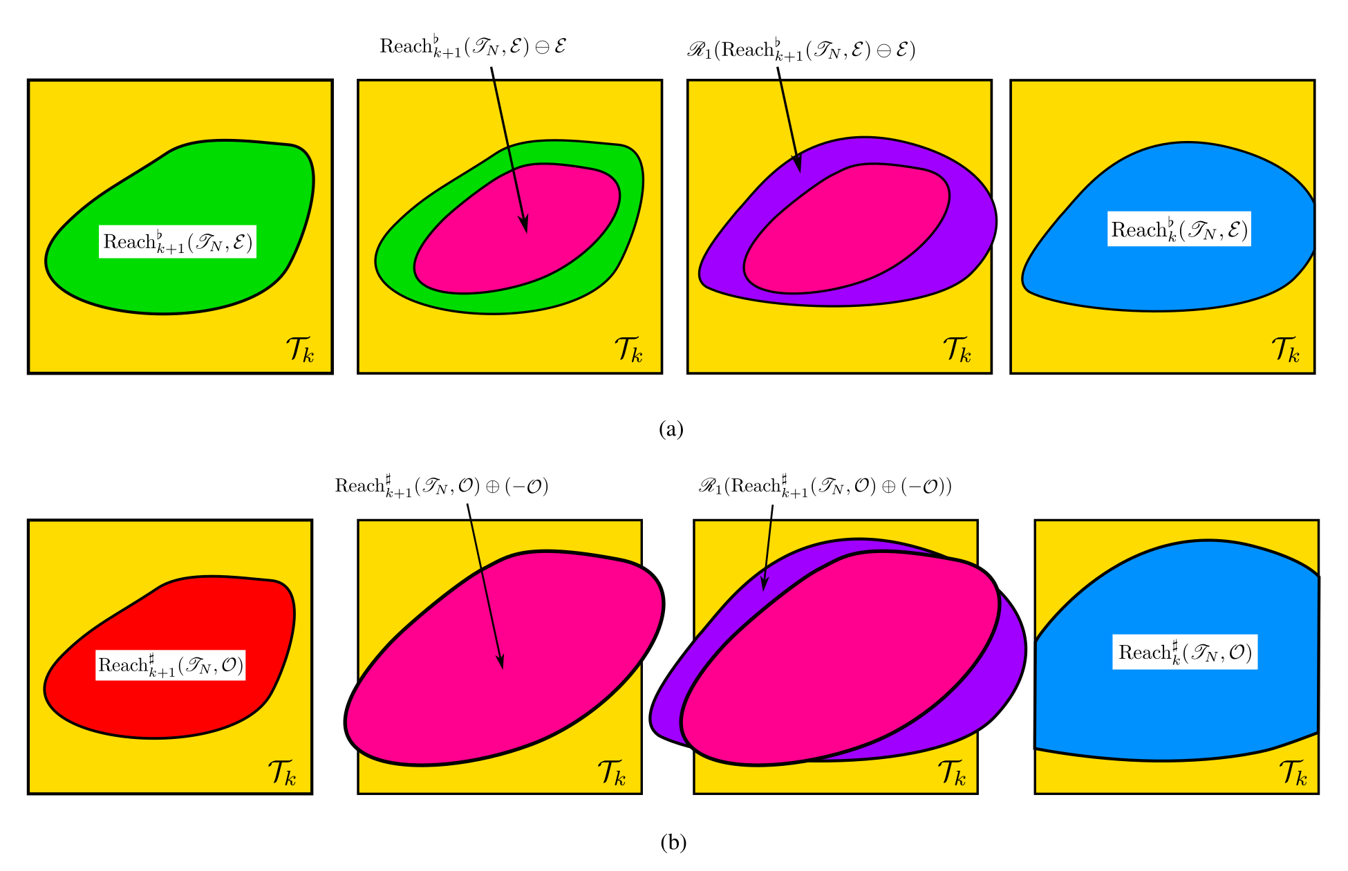
Figure 2: Graphical depiction of Lagrangian recursion methods for computing (a) the $k$-time disturbance minimal reach set, $\operatorname{Reach}_{k}^{\flat}(\operatorname{\mathscr{T}}_{N},\operatorname{\mathcal{E}})$, from $\operatorname{Reach}_{k+1}^{\flat}(\operatorname{\mathscr{T}}_{N},\operatorname{\mathcal{E}})$ via (21) and (b) the $k$-time disturbance maximal reach set, $\operatorname{Reach}_{k}^{\sharp}(\operatorname{\mathscr{T}}_{N},\operatorname{\mathcal{O}})$ from $\operatorname{Reach}_{k+1}^{\sharp}(\operatorname{\mathscr{T}}_{N},\operatorname{\mathcal{O}})$ via (31).

Theorem 6.

For the system given in (1), the $k$-time disturbance maximal reach set $\operatorname{Reach}_{k}^{\sharp}(\operatorname{\mathscr{T}}_{N},\operatorname{\mathcal{O}})$ can be computed using the recursion for $k\in\mathbb{N},k<N$:

$$\operatorname{Reach}_{N}^{\sharp}(\operatorname{\mathscr{T}}_{N},\operatorname{\mathcal{O}}) =\operatorname{\mathcal{T}}_{N}$$ (30)

$$\operatorname{Reach}_{k}^{\sharp}(\operatorname{\mathscr{T}}_{N},\operatorname{\mathcal{O}}) =\operatorname{\mathcal{T}}_{k}\cap\mathscr{R}_{1,k}(\operatorname{Reach}_{k+1}^{\sharp}(\operatorname{\mathscr{T}}_{N},\operatorname{\mathcal{O}})\operatorname{\oplus}(-\operatorname{\mathcal{O}}))$$ (31)

Proof: Again, we prove this by induction. Starting with the base case, $k=N-1$,

$$\operatorname{\mathcal{T}}_{N-1}\,\cap\, \mathscr{R}_{1,N-1}(\operatorname{Reach}_{N}^{\sharp}(\operatorname{\mathscr{T}}_{N},\operatorname{\mathcal{O}})\operatorname{\oplus}(-\operatorname{\mathcal{O}}))$$

$$=\operatorname{\mathcal{T}}_{N-1}\cap\,\mathscr{R}_{1,N-1}(\operatorname{\mathcal{T}}_{N}\operatorname{\oplus}(-\operatorname{\mathcal{O}}))$$ (32)

$$=\operatorname{\mathcal{T}}_{N-1}\cap\,\big{\{}x^{-}\in\operatorname{\mathcal{X}}:\exists\nu\in\mathcal{F},\exists w_{N-1}\in\operatorname{\mathcal{O}}$$

$$\hskip 56.9055ptf_{N-1}(x^{-},\nu(x^{-}))+w_{N-1}\in\operatorname{\mathcal{T}}_{N}\big{\}}$$ (33)

$$=\big{\{}x_{N-1}\in\operatorname{\mathcal{T}}_{N-1}:\exists\nu_{N-1}\in\mathcal{F},\exists w_{N-1}\in\operatorname{\mathcal{O}},$$

$$\hskip 56.9055ptf_{N-1}(x_{N-1},\nu(x_{N-1}))+w_{N-1}\in\operatorname{\mathcal{T}}_{N}\big{\}}$$ (34)

$$=\big{\{}x_{N-1}\in\operatorname{\mathcal{T}}_{N-1}:\exists\nu_{N-1}\in\mathcal{F},\exists w_{N-1}\in\operatorname{\mathcal{O}},$$

$$\hskip 91.04872ptx_{N}\in\operatorname{\mathcal{T}}_{N}\big{\}}$$ (35)

$$=\operatorname{Reach}_{N-1}^{\sharp}(\operatorname{\mathscr{T}}_{N},\operatorname{\mathcal{O}}).$$ (36)

For any $k\in\operatorname{\mathbb{N}}$, $k<N-1$

$$\operatorname{\mathcal{T}}_{k}\,\cap\, \mathscr{R}_{1,k}(\operatorname{Reach}_{k+1}^{\sharp}(\operatorname{\mathscr{T}}_{N},\operatorname{\mathcal{O}})\operatorname{\oplus}(-\operatorname{\mathcal{O}}))$$

$$=\big{\{}x_{k}\in\operatorname{\mathcal{T}}_{k}:\exists\nu_{k}\in\mathcal{F},\exists w_{k}\in\operatorname{\mathcal{O}},$$

$$\hskip 42.67912ptf_{k}(x_{k},\nu(x_{k}))+w_{k}\in\operatorname{Reach}_{k+1}^{\sharp}(\operatorname{\mathscr{T}}_{N},\operatorname{\mathcal{O}})\big{\}}$$ (37)

$$=\big{\{}x_{k}\in\operatorname{\mathcal{T}}_{k}:\exists\nu_{k}\in\mathcal{F},\exists w_{k}\in\operatorname{\mathcal{O}},$$

$$\hskip 42.67912ptx_{k+1}\in\operatorname{Reach}_{k+1}^{\sharp}(\operatorname{\mathscr{T}}_{N},\operatorname{\mathcal{O}})\big{\}}.$$ (38)

By expanding $\operatorname{Reach}_{k+1}^{\sharp}(\operatorname{\mathscr{T}}_{N},\operatorname{\mathcal{O}})$ with its definition (7),

$$=\big{\{}x_{k}\in\operatorname{\mathcal{T}}_{k}:\forall t\in\operatorname{\mathbb{N}}_{[k,N-1]},\exists\nu_{t}\in\mathcal{F},\hskip 17.07182pt$$

$$\hskip 58.04343pt\exists w_{t}\in\operatorname{\mathcal{O}},x_{t+1}\in\operatorname{\mathcal{T}}_{t+1}\big{\}}$$

$$=\operatorname{Reach}_{k}^{\sharp}(\operatorname{\mathscr{T}}_{N},\operatorname{\mathcal{O}})$$ (39)

which completes the proof.   

Figure 2 shows, graphically, the recursion process for the disturbance minimal and maximal reach sets.

We synthesize the recursions shown in Theorems 2 and 3 into algorithmic forms, see Algorithms 1 and 2. These algorithms compute the robust and augmented effective target sets which have been shown to approximate the stochastic effective $\alpha$-level set.

Input : Target tube $\operatorname{\mathscr{T}}_{N}$; system dynamics; desired probability level $\alpha\in[0,1]$; a bounded disturbance sets, $\operatorname{\mathcal{E}}$; horizon length, $N$

Output : Augmented effective target set, $\operatorname{Reach}_{0}^{\flat}(\operatorname{\mathscr{T}}_{N},\operatorname{\mathcal{E}})$

$\operatorname{Reach}_{N}^{\flat}(\operatorname{\mathscr{T}}_{N},\operatorname{\mathcal{E}})\leftarrow\mathcal{T}_{N}$,

for $i=N-1,N-2,\dots,0$ do

       // from (21)

       $S\leftarrow\operatorname{Reach}_{i+1}^{\flat}(\operatorname{\mathscr{T}}_{N},\operatorname{\mathcal{E}})\operatorname{\ominus}\operatorname{\mathcal{E}}$

       $E\leftarrow\mathscr{R}_{1,k}(S)$

       $\operatorname{Reach}_{i}^{\flat}(\operatorname{\mathscr{T}}_{N},\operatorname{\mathcal{E}})\leftarrow\mathcal{T}_{i}\cap E$

      

end for

Algorithm 1 Recursion for the disturbance minimal reach set.

Input : Target tube $\operatorname{\mathscr{T}}_{N}$; system dynamics; desired probability level $\alpha\in[0,1]$; a bounded disturbance sets, $\operatorname{\mathcal{O}}$; horizon length, $N$

Output : Robust effective target set, $\operatorname{Reach}_{0}^{\sharp}(\operatorname{\mathscr{T}}_{N},\operatorname{\mathcal{O}})$

$\operatorname{Reach}_{N}^{\sharp}(\operatorname{\mathscr{T}}_{N},\operatorname{\mathcal{O}})\leftarrow\mathcal{T}_{N}$,

for $i=N-1,N-2,\dots,0$ do

       // from (31)

       $S\leftarrow\operatorname{Reach}_{i+1}^{\sharp}(\operatorname{\mathscr{T}}_{N},\operatorname{\mathcal{O}})\operatorname{\oplus}(-\operatorname{\mathcal{O}})$

       $E\leftarrow\mathscr{R}_{1,k}(S)$

       $\operatorname{Reach}_{i}^{\sharp}(\operatorname{\mathscr{T}}_{N},\operatorname{\mathcal{O}})\leftarrow\mathcal{T}_{i}\cap E$

      

end for

Algorithm 2 Recursion for the disturbance maximal reach set.

4.3 Min-max formulation for $\operatorname{Reach}_{k}^{\flat}(\operatorname{\mathscr{T}}_{N},\operatorname{\mathcal{E}})$

A min-max optimal control problem was presented in [22, Sec. 1], [30, Sec. 4.6.2] to compute the disturbance minimal reach set for the system (1). The optimization problem is:

(Min-max problem for robust effective target sets)

$$\begin{array}[]{rl}\underset{\rho\in\mathcal{P}}{\mbox{minimize}}&\hskip-5.69046pt\underset{\bar{w}_{[0,N-1]}\in\operatorname{\mathcal{E}}^{N}}{\mbox{ maximize}}\ J(\rho,\bar{w}_{[0,N-1]};x_{0})\\ \mbox{subject to}&\hskip-8.5359pt\left\{\begin{array}[]{rll}x_{k+1}&=f(x_{k},\nu_{k}(x_{k}))+w_{k},&\quad k\in\mathbb{N}_{[0,N-1]}\\ \nu_{k}(\cdot)&\in\mathcal{F}&\quad k\in\mathbb{N}_{[0,N-1]}\\ \rho&=[\nu_{0}(\cdot)\ \ldots\ \nu_{N-1}(\cdot)]\\ \bar{w}_{[0,N-1]}&=[w_{0}\ \ldots\ w_{N-1}(\cdot)]\\ \end{array}\right.\end{array}$$ (40g)

$$\hskip 75.0001ptg_{k}(x_{k})\triangleq 1-\boldsymbol{1}_{\mathcal{T}_{k}}(x_{k}),\ k\in\operatorname{\mathbb{N}}_{[0,N]}$$ (40h)

$$J(\rho,\bar{w}_{[0,N-1]};x_{0})=\sum\limits_{k=0}^{N}g_{k}(x_{k})$$ (40i)

where the decision variables are $\rho$ and $\bar{w}_{[0,N-1]}$. The min-max optimal control problem (40) can be solved using dynamic programming [30, Sec 1.6]. We generate the cost-to-go/value functions $J^{\ast}_{k}(x):\mathcal{X}\rightarrow\operatorname{\mathbb{N}}_{[0,N-k+1]}$ for $k\in\operatorname{\mathbb{N}}_{[0,N]}$ with the optimal value of problem (40) when starting at $x_{0}$ as $J^{\ast}_{0}(x_{0})$. We define $J^{\ast}_{N}(x)=g_{N}(x)$, and obtain the remaining value functions via a dynamic programming recursion,

$$H^{\ast}_{k}(u,x) =\sup_{w\in\operatorname{\mathcal{E}}}\left[J^{\ast}_{k+1}(f(x,u)+w)+g_{k}(x)\right]$$ (41a)

$$J^{\ast}_{k}(x) =\inf_{u\in\operatorname{\mathcal{U}}}H^{\ast}_{k}(u,x).$$ (41b)

Note that here $J^{\ast}_{k}(x)$ records the minimum count of violations of the target tube constraint by the system (1) when starting at $x$ at time $k$ under the optimal choice of the inputs $\nu_{k}(\cdot)$ and adversarial choice of the disturbances $w_{k}$ [30, Sec. 4.6.2]. This follows from (40h), where $x_{k}\not\in\operatorname{\mathcal{T}}_{k}$ if and only if $g_{k}(x_{k})=1$ and $x_{k}\in\operatorname{\mathcal{T}}_{k}$ if and only if $g_{k}(x_{k})=0$. By construction,

$$\operatorname{Reach}_{0}^{\flat}(\operatorname{\mathscr{T}}_{N},\operatorname{\mathcal{E}}) =\{x\in\mathcal{X}:J^{\ast}_{0}(x_{0})=0\}.$$ (42)

Remark 2.

A min-min problem can be similarly constructed for the disturbance maximal reach set for system (1). Here, the system is driven to stay within the target tube with the input’s optimal efforts augmented by the disturbance.

4.4 Proof of Theorem 1

Theorem 1 states for systems (1) that satisfies Assumption 1, there exists an optimal Markov policy $\pi^{\ast}$ associated with the set $\operatorname{Reach}_{0}^{\flat}(\operatorname{\mathscr{T}}_{N},\operatorname{\mathcal{E}})$, i.e.. we want to show that there is an optimal policy for (40) $\pi^{\ast}\in\mathcal{M}\subset\mathcal{P}$. We will prove this using the equivalent min-max problem formulated in Section 4.3.

The organization of the proof is as follows: first, we will show that $g_{k}$ are l.s.c. over $\operatorname{\mathcal{X}}$. Then, we will show that, for every $k\in\mathbb{Z}_{[0,N-1]}$, the functions $J_{k}^{\ast}$ and $H_{k}^{\ast}$ of (40) are l.s.c. over $\operatorname{\mathcal{X}}$ and $\operatorname{\mathcal{X}}\times\operatorname{\mathcal{U}}$ respectively, and that there exists a Borel-measurable (and therefore universally measurable [28, Definition 7.20]) state-feedback control law $\mu_{k}^{\ast}(\cdot)$. We thus construct an optimal Markov policy $\pi^{\ast}\triangleq[\mu_{0}^{\ast}(\cdot)\ \ldots\ \mu_{N-1}^{\ast}(\cdot)]$ associated with $\operatorname{Reach}_{0}^{\flat}(\operatorname{\mathscr{T}}_{N},\operatorname{\mathcal{E}})$, completing the proof.

Since the target tube $\operatorname{\mathscr{T}}_{N}$ is closed, $-\boldsymbol{1}_{\operatorname{\mathcal{T}}_{k}}$ is l.s.c. over $\operatorname{\mathcal{X}}$ by (P1). We conclude that $g_{k}$ is l.s.c. over $\operatorname{\mathcal{X}}$ for $k\in\mathbb{Z}_{[0,t]}$ by the fact that constant functions are l.s.c., (P2), and (40h).

Next, we prove the l.s.c. property of $J_{k}^{\ast}$ and $H_{k}^{\ast}$ and the existence of a Borel-measurable $\nu_{k}^{\ast}(\cdot)$ by induction. Consider the base case $k=N-1$. From (41a),

$$H_{N-1}^{\ast}(u,x) =\sup_{w_{N-1}\in\operatorname{\mathcal{E}}}[J_{N}(f(x,u)+w_{N-1})+g_{N-1}(x)]$$

$$=\sup_{w_{N-1}\in\operatorname{\mathcal{E}}}[g_{N}(f(x,u)+w_{N-1})+g_{N-1}(x)]$$ (43)

Since $f$ is continuous over $\operatorname{\mathcal{X}}\times\operatorname{\mathcal{U}}$, $g_{N}(f(x,u)+w_{N-1})$ is l.s.c. over $\operatorname{\mathcal{X}}\times\operatorname{\mathcal{U}}\times\mathcal{W}$ by the fact that $g_{N}$ is l.s.c. over $\mathcal{X}$ and (P3). This implies that the objective in (43) is l.s.c. by the fact that $g_{N-1}$ is l.s.c. over $\operatorname{\mathcal{X}}$ and (P2). Hence, $H_{N-1}^{\ast}(u,x)$ is l.s.c. over $\operatorname{\mathcal{X}}\times\operatorname{\mathcal{U}}$ by (P4). Additionally, since $\operatorname{\mathcal{U}}$ is compact and $H_{N-1}^{\ast}(u,x)$ is l.s.c., $J_{N-1}^{\ast}(x)$ is l.s.c. over $\mathcal{X}$ and there exists a Borel-measurable state-feedback law $\mu_{N-1}(x)$ that optimizes (41b) by (P5). This completes the proof of the base case.

Assume, for induction, the case $k=t,\ t\in\mathbb{N}_{[0,N-2]}$ is true, i.e, $J_{t}^{\ast}$ is lower semicontinuous. Then, by the same arguments as above, we conclude that $J_{t-1}^{\ast}$ and $H_{t-1}^{\ast}$ is l.s.c. over $\operatorname{\mathcal{X}}$ and $\operatorname{\mathcal{X}}\times\operatorname{\mathcal{U}}$, and a Borel-measurable state-feedback law $\mu_{t-1}^{\ast}(x)$ exists via (P2)–(P5), and (41). This completes the induction, and demonstrates the existence of $\pi^{\ast}$ associated with $\operatorname{Reach}_{0}^{\flat}(\operatorname{\mathscr{T}}_{N},\operatorname{\mathcal{E}})$.

5 Improving Approximations With Multiple Bounded Disturbance Sets

Theorem 4 demonstrates that the disturbance minimal and maximal reach sets are a under and overapproximation, respectively, of the stochastic reach set. These sets are computed using bounded disturbance sets $\operatorname{\mathcal{E}}$, and $\operatorname{\mathcal{O}}$. These disturbance sets, however, are not unique (Remark 1) and many different disturbance sets can satisfy the sufficient conditions established in Section 3.

In this section we will demonstrate how we can use many different bounded disturbance sets $\operatorname{\mathcal{E}}_{i}$, $\operatorname{\mathcal{O}}_{i}$, $i\in\{1,\dots,M\}$, we can combine the these reach sets to help improve the approximation. For this we will assume that $\operatorname{\mathcal{E}}_{i}$, $\operatorname{\mathcal{O}}_{i}$ satisfy the conditions established in Theorem 4 for each $i\in\{1,\dots,M\}$. We will denote the disturbance minimal and maximal reach sets using $\operatorname{\mathcal{E}}_{i}$, $\operatorname{\mathcal{O}}_{i}$ as $\operatorname{Reach}_{k}^{\flat}(\operatorname{\mathscr{T}}_{N},\operatorname{\mathcal{E}}_{i})$ and $\operatorname{Reach}_{k}^{\sharp}(\operatorname{\mathscr{T}}_{N},\operatorname{\mathcal{O}}_{i})$, respectively.

5.1 Tighter approximations via multiple disturbance sets

We first examine how to improve the underapproximation using multiple disturbance minimal reach sets computed using $\operatorname{\mathcal{E}}_{i}$. Algorithm 3, Theorems 7 and 8, and Lemma 48 demonstrate these techniques.

Theorem 7.

Let $\operatorname{\mathcal{E}}_{i}$, be a bounded set which satisfies the condition

$$\operatorname{\mathbb{P}}\left(\bar{w}_{[k,N-1]}\in\operatorname{\mathcal{E}}_{i}^{N-k}\right)=\alpha$$ (44)

for all $i\in\operatorname{\mathbb{N}}_{[1,M]}$, $\bar{w}_{[k,N-1]}=[w_{k},w_{k+1},\dots w_{N-1}]$. For a nonlinear system (1), the union of each disturbance minimal reach set is a subset of the true stochastic reach set, i.e.

$$\operatorname{Reach}_{k}^{\flat+}(\operatorname{\mathscr{T}}_{N},\operatorname{\mathcal{E}}_{[1,M]})=\bigcup_{m=1}^{M}\operatorname{Reach}_{k}^{\flat}(\operatorname{\mathscr{T}}_{N},\operatorname{\mathcal{E}}_{m})\subseteq\operatorname{\mathcal{L}}_{k}.$$ (45)

Proof: From 4 $\operatorname{Reach^{\flat}}_{k}(\operatorname{\mathscr{T}}_{N},\operatorname{\mathcal{E}}_{i})\subseteq\operatorname{\mathcal{L}}_{k}$ for each $i\in\operatorname{\mathbb{N}}_{[1,N]}$. Thus the union of these sets remains a subset of $\operatorname{\mathcal{L}}_{k}$.   

Theorem 8.

Let $\operatorname{\mathcal{E}}_{i}$, be a bounded set which satisfies the condition

$$\operatorname{\mathbb{P}}\left(\bar{w}_{[k,N-1]}\in\operatorname{\mathcal{E}}_{i}^{N-k}\right)=\alpha$$ (46)

for all $i\in\operatorname{\mathbb{N}}_{[1,M]}$, $\bar{w}_{[k,N-1]}=[w_{k},w_{k+1},\dots w_{N-1}]$. For a linear system (2), if $\mathcal{U}$ is convex and compact, $\operatorname{\mathscr{T}}_{N}$ is closed and convex, and $Q(\cdot|x,u)$ is continuous and log-concave, then the convex hull of the robust reach avoid set for each bounded disturbance $\operatorname{Reach^{\flat}}_{k}(\operatorname{\mathscr{T}}_{N},\operatorname{\mathcal{E}}_{i})$, is a subset of the true reach-avoid level set $\operatorname{\mathcal{L}}_{k}$, i.e.

$$\operatorname{Reach}_{k}^{\flat+}(\operatorname{\mathscr{T}}_{N},\operatorname{\mathcal{E}}_{[1,M]})=\mathrm{Co}\big{(}\bigcup_{m=1}^{M}\operatorname{Reach}_{k}^{\flat}(\operatorname{\mathscr{T}}_{N},\operatorname{\mathcal{E}}_{m})\big{)}\subseteq\operatorname{\mathcal{L}}_{k}.$$ (47)

Proof: From 4 $\operatorname{Reach}_{k}^{\flat}(\operatorname{\mathscr{T}}_{N},\operatorname{\mathcal{E}}_{i})\subseteq\operatorname{\mathcal{L}}_{k}$ for each $i\in\operatorname{\mathbb{N}}_{[1,M]}$, and from [13, Theorem 4], $\operatorname{\mathcal{L}}_{k}$ is convex. Thus, the convex hull of disturbance minimal reach sets is a subset of $\operatorname{\mathcal{L}}_{k}$ [31, Section 2.3.4].   

Lemma 1.

Let $\operatorname{\mathcal{E}}_{j}$ be a bounded set in the collection $\operatorname{\mathcal{E}}_{1},\dots,\operatorname{\mathcal{E}}_{M}$, $M,j\in\operatorname{\mathbb{N}}$, $j<M$. Then

$$\operatorname{Reach}_{k}^{\flat}(\operatorname{\mathscr{T}}_{N},\operatorname{\mathcal{E}}_{j})\subseteq\operatorname{Reach}_{k}^{\flat+}(\operatorname{\mathscr{T}}_{N},\operatorname{\mathcal{E}}_{[1,M]})$$ (48)

Proof: For a nonlinear system (1), for any $x\in\operatorname{Reach}_{k}^{\flat}(\operatorname{\mathscr{T}}_{N},\operatorname{\mathcal{E}}_{j})$, $x\in\operatorname{Reach}_{k}^{\flat+}(\operatorname{\mathscr{T}}_{N},\operatorname{\mathcal{E}}_{[1,M]})$ by (45), and for a linear system (2) any $y\in\operatorname{Reach}_{k}^{\flat}(\operatorname{\mathscr{T}}_{N},\operatorname{\mathcal{E}}_{j})$, $y\in\operatorname{Reach}_{k}^{\flat+}(\operatorname{\mathscr{T}}_{N},\operatorname{\mathcal{E}}_{[1,M]})$ by (47).   

Input : Target tube $\operatorname{\mathscr{T}}$; system dynamics; desired probability level $\alpha\in[0,1]$; $M$ bounded disturbance sets, $\operatorname{\mathcal{E}}_{1},\dots,\operatorname{\mathcal{E}}_{M}$; horizon length, $N$

Output : $N$-time stochastic reach-avoid $\alpha$-level set underapproximation, $\operatorname{Reach}_{0}^{\flat+}(\operatorname{\mathscr{T}}_{N},\operatorname{\mathcal{E}}_{[1,M]})$

// Initialization

for $m=1,2,\dots,M$ do

       $\operatorname{Reach}_{N}^{\flat}(\operatorname{\mathscr{T}}_{N},\operatorname{\mathcal{E}}_{m})\leftarrow\mathcal{T}_{N}$

end for

// Recursion

for $i=N-1,N-2,\dots,0$ do

       for $m=1,2,\dots,M$ do

             // from Algorithm 1

             $S\leftarrow\operatorname{Reach}_{i+1}^{\flat}(\operatorname{\mathscr{T}}_{N},\operatorname{\mathcal{E}}_{m})\operatorname{\ominus}\operatorname{\mathcal{E}}_{m}$

             $E\leftarrow\mathscr{R}_{1,k}(S)$

             $\operatorname{Reach}_{i}^{\flat}(\operatorname{\mathscr{T}}_{N},\operatorname{\mathcal{E}}_{m})\leftarrow\mathcal{T}_{i}\cap E$

            

       end for

      

      if nonlinear system dynamics (1) then

             $\operatorname{Reach}_{i}^{\flat+}(\operatorname{\mathscr{T}}_{N},\operatorname{\mathcal{E}}_{[1,M]})\leftarrow\bigcup_{m=1}^{M}\operatorname{Reach}_{i}^{\flat}(\operatorname{\mathscr{T}}_{N},\operatorname{\mathcal{E}}_{m}))$

       end if

      

      if linear system dynamics (2) then

             $\operatorname{Reach}_{i}^{\flat+}(\operatorname{\mathscr{T}}_{N},\operatorname{\mathcal{E}}_{[1,M]})\leftarrow\mathrm{Co}\big{(}\bigcup_{m=1}^{M}\operatorname{Reach}_{i}^{\flat}(\operatorname{\mathscr{T}}_{N},\operatorname{\mathcal{E}}_{m})\big{)}$

       end if

      

end for

Algorithm 3 Underapproximation of the stochastic effective $\alpha$-level set using multiple bounded disturbances and unions or convex hulls.

Now we apply similar methodology to demonstrate how to improve the overapproximation using multiple augmented effective target sets.

Theorem 9.

Let $\operatorname{\mathcal{O}}_{i}$, be a bounded set which satisfies the condition

$$\operatorname{\mathbb{P}}\left(\bar{w}_{[k,N-1]}\in\operatorname{\mathcal{O}}_{i}^{N-k}\right)=\alpha$$ (49)

for all $i\in\operatorname{\mathbb{N}}_{[1,M]}$, $\bar{w}_{[k,N-1]}=[w_{k},w_{k+1},\dots w_{N-1}]$. For a nonlinear system (1), the union of each robust reach avoid set is a subset of the true reach-avoid level set, i.e.

$$\operatorname{Reach}_{k}^{\sharp+}(\operatorname{\mathscr{T}}_{N},\operatorname{\mathcal{O}}_{[1,M]})=\bigcap_{m=1}^{M}\operatorname{Reach}_{k}^{\sharp}(\operatorname{\mathscr{T}}_{N},\operatorname{\mathcal{O}}_{m})\supseteq\operatorname{\mathcal{L}}_{k}.$$ (50)

Proof: From 4 $\operatorname{Reach\raisebox{2.0pt}{${}^{\sharp}$}}_{k}(\operatorname{\mathscr{T}}_{N},\operatorname{\mathcal{O}}_{i})\supseteq\operatorname{\mathcal{L}}_{k}$ for each $i\in\operatorname{\mathbb{N}}_{[1,N]}$. Thus the intersection of these sets remains a subset of $\operatorname{\mathcal{L}}_{k}$.   

Lemma 2.

Let $\operatorname{\mathcal{O}}_{j}$ be a bounded set in the collection $\operatorname{\mathcal{O}}_{1},\dots,\operatorname{\mathcal{O}}_{M}$, $M,j\in\operatorname{\mathbb{N}}$, $j<M$. Then

$$\operatorname{Reach}_{k}^{\sharp+}(\operatorname{\mathscr{T}}_{N},\operatorname{\mathcal{O}}_{[1,M]})\subseteq\operatorname{Reach\raisebox{2.0pt}{${}^{\sharp}$}}_{k}(\operatorname{\mathscr{T}}_{N},\operatorname{\mathcal{O}}_{j})$$ (51)

Proof: From the intersection operation in (50), clearly $\operatorname{Reach}_{k}^{\sharp+}(\operatorname{\mathscr{T}}_{N},\operatorname{\mathcal{O}}_{[1,M]})\subseteq\operatorname{Reach\raisebox{2.0pt}{${}^{\sharp}$}}_{k}(\operatorname{\mathscr{T}}_{N},\operatorname{\mathcal{O}}_{j})$ for any $j\in\{1,\dots,M\}$.   

The methods from Theorem 9 and Lemma 2 are succinctly combined in Algorithm 4.

Input : Target tube $\operatorname{\mathscr{T}}$; system dynamics; desired probability level $\alpha\in[0,1]$; $M$ bounded disturbance sets, $\operatorname{\mathcal{E}}_{1},\dots,\operatorname{\mathcal{E}}_{M}$; horizon length, $N$

Output : $N$-time stochastic reach-avoid $\alpha$-level set underapproximation, $\operatorname{Reach}_{0}^{\sharp+}(\operatorname{\mathscr{T}}_{N},\operatorname{\mathcal{O}}_{[1,M]})$

// Initialization

for $m=1,2,\dots,M$ do

       $\operatorname{Reach}_{N}^{\sharp}(\operatorname{\mathscr{T}}_{N},\operatorname{\mathcal{O}}_{m})\leftarrow\mathcal{T}_{N}$

end for

// Recursion

for $i=N-1,N-2,\dots,0$ do

       for $m=1,2,\dots,M$ do

             // from Algorithm 2

             $S\leftarrow\operatorname{Reach}_{i+1}^{\sharp}(\operatorname{\mathscr{T}}_{N},\operatorname{\mathcal{O}}_{m})\operatorname{\oplus}(-\operatorname{\mathcal{O}}_{m})$

             $E\leftarrow\mathscr{R}_{1,k}(S)$

             $\operatorname{Reach}_{i}^{\sharp}(\operatorname{\mathscr{T}}_{N},\operatorname{\mathcal{O}}_{m})\leftarrow\mathcal{T}_{k}\cap E$

            

       end for

      

      if nonlinear system dynamics (1) then

             $\operatorname{Reach}_{i}^{\sharp+}(\operatorname{\mathscr{T}}_{N},\operatorname{\mathcal{O}}_{[1,M]})\leftarrow\bigcap_{m=1}^{M}\operatorname{Reach}_{i}^{\sharp}(\operatorname{\mathscr{T}}_{N},\operatorname{\mathcal{O}}_{m})$

       end if

      

end for

Algorithm 4 Overapproximation of the stochastic effective $\alpha$-level set using multiple bounded disturbances and intersections.

6 Computation of disturbance subsets: $\operatorname{\mathcal{E}},\operatorname{\mathcal{O}}$

With the sufficient conditions established for $\operatorname{\mathcal{E}},\operatorname{\mathcal{O}}$ in Theorem 4 we now focus our attention on methods for computing bounded disturbance sets that satisfy these criteria. To reiterate, our disturbance in (1), $w_{k}$ is an assumed i.i.d. disturbance drawn from the probability space $(\operatorname{\mathcal{W}},\sigma(\operatorname{\mathcal{W}}),\operatorname{\mathbb{P}}_{w_{k}})$. As mentioned in Remark 1, these bounded disturbance sets need not be unique. Thus, there are many different methods that can be used to these bounded sets. Here we propose an optimization problem to obtain generic polyhedra that can be used to represent the bounded sets.

First, we define a polytope

$$\hbox{Poly}(A,b)=\big{\{}y\in\operatorname{\mathbb{R}}^{p}:Ay\preceq b\}$$ (52)

where $A\in\operatorname{\mathbb{R}}^{q\times p}$, $b\in\operatorname{\mathbb{R}}^{q}$, and $y\preceq b$ if $y_{i}\leq b_{i}$ for all $i\in\{1,\dots,p\}$. For a fixed polytopic shape, i.e. a fixed $A$, we formulate the optimization problem,

$$\mathmakebox[\widthof{$\underset{\displaystyle b}{\mathrm{subject~{}to}}$}]{\underset{\displaystyle b}{\mathrm{minimize}}}\quad\log(\mathrm{vol}(\hbox{Poly}(A,b)))$$ (53a)

$$\mathmakebox[\widthof{$\underset{\displaystyle\phantom{b}}{\mathrm{\,subject~{}to}}$}][c]{\mathmakebox[\widthof{$\mathrm{minimize}$}][l]{\mathrm{subject~{}to}}}\quad \gamma^{\frac{1}{N}} \leq\operatorname{\mathbb{P}}_{w}(w_{k}\in\hbox{Poly}(A,b))$$ (53b)

To obtain $\operatorname{\mathcal{E}}$ we use $\gamma=\alpha$, and for $\operatorname{\mathcal{O}}$, $\gamma=1-\alpha$. The volume $\mathrm{vol}$ is the Lebesgue measure of the set,

$$\mathrm{vol}(A)=\int_{A}dx.$$

Lemma 3.

For $\theta\in[0,1]$, and $A\in\operatorname{\mathbb{R}}^{q\times p}$ such that $\hbox{Poly}(A,0)=\{0\}$, then $\hbox{Poly}(A,\theta b)=\theta\hbox{Poly}(A,b)$.

Proof: For $\theta=0$, $\hbox{Poly}(A,0)=0\times\hbox{Poly}(A,b)=\{0\}.$

For $\theta\in(0,1]$, if $y\in\hbox{Poly}(A,\theta b)$ then $Ay\leq\theta b\Rightarrow Ay/\theta\leq b\Rightarrow y\in\theta\hbox{Poly}(A,b)$. Thus $\hbox{Poly}(A,\theta b)\subseteq\theta\hbox{Poly}(A,b)$.

If $y\in\hbox{Poly}(A,b)$, then $Ay\leq b\Rightarrow A\theta y\leq\theta b$. Let $z=\theta y$, then $z\in\hbox{Poly}(A,\theta b)\Rightarrow\theta\hbox{Poly}(A,b)\subseteq\hbox{Poly}(A,\theta b)$.   

Proposition 2.

For $A\in\operatorname{\mathbb{R}}^{q\times p}$ such that $\hbox{Poly}(A,0)=\{0\}$, if $\operatorname{\mathbb{P}}_{w}$ is a log-concave probability measure, then (53) is a concave minimization problem.

Proof: From [31, Ex. 3.44], $\mathrm{vol}(\hbox{Poly}(A,b))$ is log-concave in $b\in\operatorname{\mathbb{R}}^{p}$, implying the objective (53a) is concave.

Next we show that, for $\theta\in[0,1]$, and $b_{1},b_{2}\in\operatorname{\mathbb{R}}^{q}$,

$$\hbox{Poly}(A,\theta b_{1})\operatorname{\oplus}\hbox{Poly}(A,(1-\theta)b_{2})\subset\hbox{Poly}(A,\theta b_{1}+(1-\theta)b_{2}).$$

Let $z_{1}\in\hbox{Poly}(A,\theta b_{1})$ and $z_{2}\in\hbox{Poly}(A,(1-\theta)b_{2})$. Let $y=z_{1}+z_{2}$, hence $y\in\hbox{Poly}(A,\theta b_{1})\operatorname{\oplus}\hbox{Poly}(A,(1-\theta)b_{2})\Rightarrow Ay=Az_{1}+Az_{2}\leq\theta b_{1}+(1-\theta)b_{2}\Rightarrow y\in\hbox{Poly}(A,\theta b_{1}+(1-\theta)b_{2})$.

Now,

$$\operatorname{\mathbb{P}}_{w_{k}}\big{(}w_{k}\in\hbox{Poly}(A,\theta b_{1}+(1-\theta)b_{2})\big{)}$$

$$\hskip 28.45274pt\geq\operatorname{\mathbb{P}}_{w_{k}}\big{(}w_{k}\in\hbox{Poly}(A,\theta b_{1})\operatorname{\oplus}\hbox{Poly}(A,(1-\theta)b_{2})\big{)}$$

$$\hskip 28.45274pt=\operatorname{\mathbb{P}}_{w_{k}}\big{(}w_{k}\in\theta\hbox{Poly}(A,b_{1})\operatorname{\oplus}(1-\theta)\hbox{Poly}(A,b_{2})\big{)}$$ (54)

$$\hskip 28.45274pt\geq\operatorname{\mathbb{P}}_{w_{k}}\big{(}w_{k}\in\hbox{Poly}(A,b_{1})\big{)}^{\theta}\operatorname{\mathbb{P}}_{w_{k}}\big{(}w_{k}\in\hbox{Poly}(A,b_{2})\big{)}^{1-\theta}.$$ (55)

Equation (54) follows from Lemma 3 and (55) follows from the log-concavity of $\operatorname{\mathbb{P}}_{w_{k}}$. Since log-concavity implies quasiconcavity, the constraint (53b) is convex. Thus, the problem (53) minimizes a concave function over a convex set.

 

Corollary 1.

For $A\in\operatorname{\mathbb{R}}^{q\times p}$, and polytope

$$\hbox{Poly}(A,b,c)=\big{\{}y\in\operatorname{\mathbb{R}}^{p}:A(y-c)\preceq b\big{\}}$$ (56)

where $\hbox{Poly}(A,0,c)=\{c\}$, if $\operatorname{\mathbb{P}}_{w}$ is a log-concave probability measure, then (53) is a concave minimization problem.

Proof: Note that $\hbox{Poly}(A,b,c)=\hbox{Poly}(A,b)\operatorname{\oplus}\{c\}$. Let $v_{k}=w_{k}-c$, and the proof of Proposition 2 holds for the random variable $v_{k}$.   

Multiplicative optimization problems belong to the class of concave minimization (reverse convex optimization) problems, and they have been well-studied in global optimization literature [32, 33]. They may be solved to global optimality using branch-and-bound techniques. However, we employ a computationally simple bisection method, described in Algorithm 5, to solve this problem to a potentially suboptimal solution [33, Sec. 3.3.3].

The use of generic polytopes defined by $A$, $b$, and $c$ allow for flexibility in the definition of the bounded sets. For example, if $w_{k}\sim N(\mu,\Sigma)$ then we can use Algorithm 5 to obtain a cuboid bounded set by setting $A=[\Sigma^{-1},-\Sigma^{-1}]^{\top}$, $c=\mu$, $b=[1,\dots,1]^{\top}$. If $w_{k}$ was drawn from an exponential distribution we can obtain a cuboid bounded set with $A=I$, $c=[0,\dots,0]^{\top}$, $b=[1,\dots,1]^{\top}$.

Input : Matrix, $A\in\operatorname{\mathbb{R}}^{q\times p}$, and vectors $b\in\operatorname{\mathbb{R}}^{q},c\in\operatorname{\mathbb{R}}^{p}$ defining initial Polyhedron $\hbox{Poly}(A,b,c)$, and $\gamma\in[0,1]$

Output : Polyhedral bounded disturbance set $\mathcal{S}$

$\alpha\leftarrow 1$

$p\leftarrow\operatorname{\mathbb{P}}_{w_{k}}\big{(}w_{k}\in\hbox{Poly}(A,\alpha b,c)\big{)}$

// Expansion of polyhedron to find initial values for bisection

while $p<\gamma^{\frac{1}{N}}$ do

       $\alpha\leftarrow 2\alpha$

       $p\leftarrow\operatorname{\mathbb{P}}_{w_{k}}\big{(}w_{k}\in\hbox{Poly}(A,\alpha b,c)\big{)}$

      

end while

// Bisection

if $\alpha=1$ then

       $l\leftarrow 0$

else

       $l\leftarrow\alpha/2$

      

end if

$h\leftarrow\alpha$

$m\leftarrow\frac{l+h}{2}$

$p\leftarrow\operatorname{\mathbb{P}}_{w_{k}}\big{(}w_{k}\in\hbox{Poly}(A,mb,c)\big{)}$

while $p\neq\gamma^{\frac{1}{N}}$ do

       if $p>\gamma^{\frac{1}{N}}$ then

             $h\leftarrow m$

            

      else

             $l\leftarrow m$

            

       end if

      

      $m\leftarrow\frac{l+h}{2}$

       $p\leftarrow\operatorname{\mathbb{P}}_{w_{k}}\big{(}w_{k}\in\hbox{Poly}(A,mb,c)\big{)}$

      

end while

$\mathcal{S}\leftarrow\hbox{Poly}(A,mb,c)$

Algorithm 5 Bisection algorithm for obtaining polyhedral bounded disturbance sets. If $\gamma=\alpha$, then $\mathcal{S}=\operatorname{\mathcal{E}}$, and if $\gamma=1-\alpha$, then $\mathcal{S}=\operatorname{\mathcal{O}}$.

6.1 I.i.d. Gaussian disturbances

For i.i.d. Gaussian disturbances we can determine minimum volume set satisfying (53b) in the form of an ellipsoid. If the disturbance $w_{k}$ in (1) is an $n$-dimensional Gaussian random variable with mean vector $\mu\in\operatorname{\mathbb{R}}^{n}$ and covariance matrix $\Sigma\in\operatorname{\mathbb{R}}^{n\times n}$, then its probability density function is [34, Ch. 29]

$$\psi_{w_{k}}(y)={(2\pi)}^{\frac{-n}{2}}{|\Sigma|}^{\frac{-1}{2}}\exp{\left(-\frac{{(y-\mu)}^{\top}\Sigma^{-1}{(y-\mu)}}{2}\right)},$$

$y\in\operatorname{\mathbb{R}}^{n}$.

Consider an $n$-dimensional ellipsoid, parameterized by $R^{2}\in[0,\infty)$,

$$\mathcal{Q}_{R^{2}}=\left\{y\in\operatorname{\mathbb{R}}^{n}:{(y-\mu)}^{\top}\Sigma^{-1}{(y-\mu)}\leq R^{2}\right\}.$$ (57)

For $\mu=0,\Sigma=r^{2}I_{n}$, we have $\mathcal{Q}_{R^{2}}=\{y:y^{\top}y\leq r^{2}R^{2}\}$, a $n$-dimensional hypersphere of radius $rR$. We aim to compute the parameter $R^{2}$ such that $\operatorname{\mathbb{P}}_{w_{k}}(w_{k}\in\mathcal{Q}_{R^{2}}\}=\gamma^{\frac{1}{N}}$. If $\gamma=\alpha$, then $\operatorname{\mathcal{E}}=\mathcal{Q}_{R^{2}}$ and if $\gamma=(1-\alpha)$ then $\operatorname{\mathcal{O}}=\mathcal{Q}_{R^{2}}$ will generate bounded disturbance sets that satisfy the conditions of Theorem 4.

Given a normally distributed $n$-dimensional random vector $\eta\sim\mathcal{N}(0,I_{n})$, we have $w_{k}={\Sigma}^{\frac{1}{2}}\eta+\mu$ [34, Ch. 29]. Also, $\mathcal{Q}_{R^{2}}={\Sigma}^{\frac{1}{2}}\mathcal{Q}_{\eta,R^{2}}\oplus\{\mu\}$ with $\mathcal{Q}_{\eta,R^{2}}=\{s\in\operatorname{\mathbb{R}}^{n}:s^{\top}s\leq R^{2}\}$. Since the affine transformation of $\eta$ to $w_{k}$ is deterministic, $\mathbb{P}_{w_{k}}(w_{k}\in\mathcal{Q}_{R^{2}})=\mathbb{P}_{\eta}(\eta\in\mathcal{Q}_{\eta,R^{2}})=\gamma^{\frac{1}{N}}$. From [34, Ex. 20.16], we have

$$F_{\chi^{2}(n)}(R^{2})=\mathbb{P}\left\{\chi^{2}(n)\leq R^{2}\right\}=\mathbb{P}\{\eta\in\mathcal{Q}_{\eta,R^{2}}\}=\gamma^{\frac{1}{N}}$$

where $\chi^{2}(n)$ is a chi-squared random variable with $n$ degrees of freedom and $F_{\chi^{2}(n)}(\cdot)$ denotes its cumulative distribution function. Consequently, we have

$$R^{2}=F^{-1}_{\chi^{2}(n)}\left(\gamma^{\frac{1}{N}}\right).$$ (58)

By solving (58) with $\gamma=\alpha$ or $\gamma=1-\alpha$ and then using the result in (57), we can obtain a feasible $\operatorname{\mathcal{E}}$ or $\operatorname{\mathcal{O}}$, respectively, for any Gaussian disturbance.

7 Computational challenges

Since Lagrangian methods are grid-free, they have the potential to provide substantial numerical benefits, most notably a dramatically increased computational speed and applicability to high-dimensional systems. The trade-off for the increased computational speed is a degree of conservativeness in the approximations. It was shown in [26] that for Gaussian systems with low variance, these approximations become tight to the actual solution obtained via dynamic programming. Still, there are several important computational challenges at present that can limit the efficacy of these methods for high-dimensional system analysis.

The primary challenge is the implementation of Algorithms 1 and 2 with current computational geometry methods. In particular the types of set operations required often limit the ability for current methodologies to effectively scale with increasing dimension. For linear systems, the one-step backward reach set it given by (19), thus for the disturbance maximal reach set we need intersections, Minkowski addition, and affine transformations. To compute the disturbance minimal reach set we need all the previous operations as well as Minkowski (Pontryagin) difference and, potentially, unions, or convex hulls $\mathrm{Co}(\cdot)$ if multi-disturbance set methods are used.

Table 1 summarizes various capabilities for current methodologies to perform the necessary set operations required to compute the robust and augmented effective target sets. The following subsections will provide additional detail regarding these different computational geometry methods and examine their applicability for computing the robust and augmented effective target sets.

Toolbox	MPT [16]		ET [17]		CORA
Methods	$\mathcal{H}$-polytope	$\mathcal{V}$-polytope	Ellipsoids	Support Functions	Zonotope
$\cap$	$=$		$-$	$+$, $=$	$+$
$T$	$=$	$=$	$=$	$=$	$=$
$\operatorname{\oplus}$	$=$	$=$	$+$	$=$	$=$
$\operatorname{\ominus}$	$=$		$-$
$\cup$		$=$	$+$
$\mathrm{Co}$		$=$	$+$
	[14]	[14]	[35]	[21, 14, 4]	[14]

Table 1: Computational geometry tools and their ability to perform various set operations. To compute the the disturbance maximal reach set ass the operations shaded in gray are needed. For the disturbance minimal reach set, all six operations are needed (unions and convex hulls are only required when using multiple disturbances). Each method can compute the operation exactly ($=$) or will underapproximate ($-$) or overapproximate ($+$) the result. References for the operations computability are provided at the base of the table.

7.1 Ellipsoidal Methods

Ellipsoidal methods [35, 17] can handle all of the fundamental operations previously discussed but requires that all sets be represented as ellipses. Hence for many methods—e.g. intersections, unions, Minkowski addition—this methodology cannot compute exact representations of the resulting set and thus determine approximations. For example, the intersection of two ellipses does not necessary result in an ellipse, thus ellipsoidal methods underapproximate these intersection by finding the largest ellipse that exists inside of the intersection. Conversely for unions a bounding ellipse is used to overapproximate the operation.

For the disturbance minimal and maximal reach sets these approximations make ellipsoidal methods unappealing. For the maximal reach set, we need to consistently overapproximate to maintain guarantees. However, ellipsoidal methods underapproximate intersections which makes ellipsoidal methods not applicable. Ellipsoidal methods can handle the appropriate operations for the disturbance minimal reach set, however because this computation already provides a conservative underapproximation the additional underapproximations made from the ellipsoidal methods compound the conservativeness. Hence ellipsoidal methods are not advantageous.

7.2 $\mathcal{H}$ and $\mathcal{V}$-polytopes

Perhaps the most applicable method, $\mathcal{H}$ and $\mathcal{V}$-polytopes represent polytopic sets in either halfspace or vertex form, respectively. One of the most current toolboxes for polytopic computational geometry is the Model Parametric Toolbox [16], written in MATLAB. For most set operations there are convenient ways to exactly compute the aforementioned set operation using $\mathcal{H}$ or $\mathcal{V}$-polytope representation. Many operations are only feasible for a specific representative form, e.g. intersections with $\mathcal{H}$-polytope form. Thus, to use these methods to compute the effective target sets, we must be able to switch between the two forms, which is limited by the vertex-facet enumeration problem. This problem limits ability for these methods to extend to higher-dimensional spaces as the vertex-facet problem becomes more and more costly.

Additionally polytopic representation also suffers from a need to approximation generic shapes as polytopes. For example, representing the ellipsoid computed in Section 6.1, $\mathcal{Q}_{R^{2}}$, can be problematic In order to obtain an approximation of the ellipse using either $\mathcal{H}$ or $\mathcal{V}$-polytope representations we need to to choose $m$ directions in $n$ dimensional space on the surface of the ellipse. For an underapproximation each point becomes a vertex of the polytope and as an overapproximation the plane tangential to the ellipsoid’s surface at that point becomes a halfspace. Which points on the surface would best approximate the ellipse is a hard problem but a good heuristic is to use points that are equidistant, i.e. $x_{i}^{T}x_{j}=c$ for all $i\neq j$, $c$ is some constant. Choosing equidistant vectors eliminates the possibility of creating unbounded or very large overapproximations of the ellipsoid from poor directional choice; instead unboundedness or large overapproximations would arise if $m$ is very small, especially compared to the dimension size $n$, e.g. if $m<n$. For a two-dimensional system choosing the appropriate directions is a simple problem in which $x_{i}^{T}x_{j}=\cos(2*pi/m)$, see Figure 3.

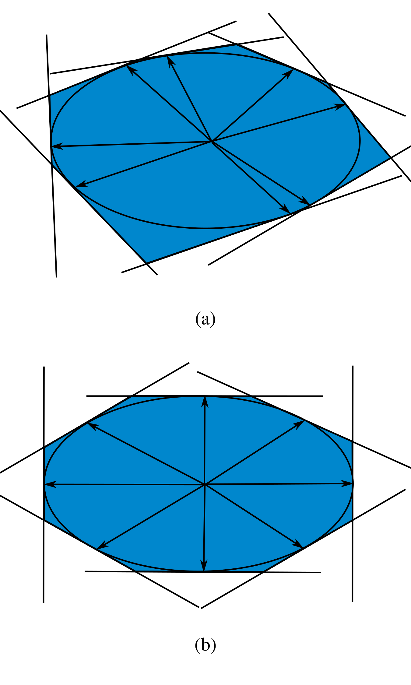
Figure 3: Ellipsoid approximations from (a) random directions (b) equidistant vector generation, $n=2$, $m=8$.

In systems with $n>2$, however, approximations are done in a random manner [36] by sampling points on the exterior of the ellipse, and hence polyhedral representations will vary.

Additionally, accurate approximations require an increasing number of vertices/halfspaces as dimensionality increases, again increasing computational requirements. The use of bounded disturbances that are constructed as simple polytopic structures, as are made in Algorithm 5, can help reduce computational difficulties in higher dimensions. In [37] it was shown that using a single disturbance box allowed for the underapproximation methods to compute simulations on a 6-dimensional chain of integrators. Additionally for low-dimensional systems the average computation time for a disturbance box was 50% of the computation time for a polytopic ellipsoid approximation.

Because the necessary set operations can be performed without additional conservativeness through approximations, we employ polytopic methods and use MPT to compute the robust effective target set in the examples.

7.3 Zonotopes

Zonotopes have been demonstrated to be effective tools for higher-dimensional reachability analysis [38]. For zonotopes, intersections are represented as zonotope bundles, and the Minkowski sum of a set and a zonotope bundle yields an overapproximation. This restricts us from using zonotopes for the disturbance minimal reach set since it would nullify our conservativeness guarantee.

Because the disturbance maximal reach set is an overapproximation zonotopes are a viable option for this computation. We do not use these methods in this paper, however, because we do not wish to compound conservativeness, i.e. take overapproximations of an overapproximation (similar to ellipsoidal methods).

7.4 Star Methods

The star methods are capable of performing undisturbed reach computations [20] but have not been reported to be able to handle the set operations individually. Hence we cannot evaluate their efficacy with our methods.

7.5 Support Functions

Support functions are a powerful tool for representing generic convex sets [39, 21, 4, 40]. They have very simple and effective methods for computing affine transformations and Minkowski summation [4, 14], and can compute Minkowski differences with a polytopic set [41]. However, intersections with support functions are more problematic. Exact computation of intersections can be determined through a computationally difficult optimization problem [14] but they can be overapproximated simply. This overapproximation eliminates their applicability for computation of the robust effective target set. Additionally, this intersection approximation does not permit additional Minkowski summation [14].

8 Examples

All calculations were done using MATLAB R2017a on a computer with an Intel Xeon E3-1270 v6 processor and 32 GB RAM (2400MHz DDR4 UDIMM ECC) running Ubuntu 16.04. The computations were performed using the Stochastic Reachability Toolbox (SReachTools) which utilizes the model parametric toolbox (MPT 3.0) [16] for the polyhedra and set operations. All simulation code can be found at https://hscl.unm.edu/software/code/.

8.1 Two-dimensional double integrator

We first consider a simple double integrator example. This example allows for a direct comparison of the conservatism of the results and a comparison of the computations speed against dynamic programming methods. The underapproximation methods were compared against dynamic programming in [26]. Here, we reiterate these results as well as demonstrate the overapproximation.

The discretized double integrator dynamics are

$$x_{k+1}=\left[\begin{array}[]{cc}1&T\\ 0&1\end{array}\right]x_{k}+\left[\begin{array}[]{c}\frac{T^{2}}{2}\\ T\end{array}\right]u_{k}+w_{k}$$ (59)

with state $x_{k}\in\operatorname{\mathcal{X}}\subseteq\operatorname{\mathbb{R}}^{2}$, input $u_{k}\in\operatorname{\mathcal{U}}\subseteq\operatorname{\mathbb{R}}$, $T=0.25$, and Gaussian disturbance $w_{k}\sim\mathcal{N}(0,0.005\cdot I_{2})$. We consider the viability problem, or equivalently the target tube problem with $\operatorname{\mathcal{T}}_{k}=\{x_{k}\in\mathcal{X}:|x_{i}|\leq 1,i\in\{1,\dots,n\}\}$ for all $k\in\{0,\dots,N\}$. In this example $\operatorname{\mathcal{E}}$ and $\operatorname{\mathcal{O}}$ are ellipsoidal sets obtained via (58) and (57) with $\alpha=0.8$.

Figure 4 compares the underapproximation and overapproximation, via Algorithms 1 and 2, to the level sets computed via dynamic programming, as in [7]. A comparison between the total computation time for both approaches is provided in Table 2. The accuracy of dynamic programming relies on its grid size, resulting in a trade-off between accuracy and computation speed, from which Algorithms 1 and 2 do not suffer.

Grid Size	Dynamic Programming	Approximations	Ratio
$41\times 41$	8.16	0.98	8.3
$82\times 82$	59.76	0.98	60.9

Table 2: Computation times, in seconds, for the double integrator problem, solved via dynamic programming and via Algorithm 1 and 2. The ratio of computation times is the computation time via dynamic programming divided by computation time via Lagrangian approximations.

Both the under and overapproximation in this example are conservative. This is the result of the need to be robust, in the case of the underapproximation, to all disturbances in a bounded set. For Gaussian disturbances, as the variance of the disturbance reduces, this bounded set also decreases in size as a direct consequence of (57). We demonstrated previously [26], omitted here for brevity, that as the variance decreases the underapproximation becomes tight to the solution obtained via dynamic programming. This result holds true for the overapproximation as well.

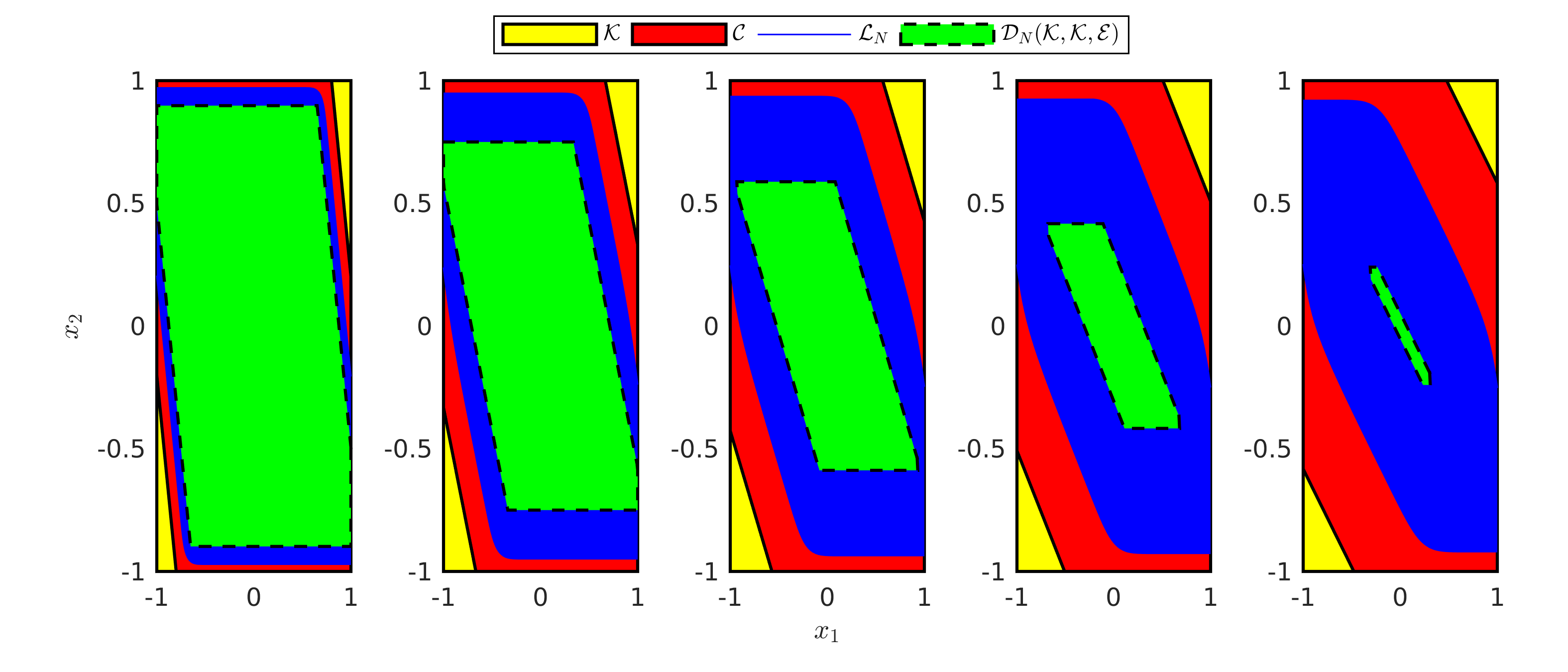
Figure 4: Double integrator example computation and comparison of $\mathcal{L}_{k}(\operatorname{\mathscr{T}}_{N},\alpha)$, $\operatorname{Reach}_{k}^{\flat}(\operatorname{\mathscr{T}}_{N},\operatorname{\mathcal{E}})$ and $\operatorname{Reach}_{k}^{\sharp}(\operatorname{\mathscr{T}}_{N},\operatorname{\mathcal{O}})$, where $\operatorname{\mathcal{E}}$ and $\operatorname{\mathcal{O}}$ are ellipsoidal sets. Here, $N=5$ and, from left to right, $k=4,3,2,1,0$.

8.2 Chain of integrators

As was mentioned in 7.2 because ellipsoidal representations of polytopes can require high numbers of vertices or facets to represent as the dimension of the system increases it is often advantageous, from a computational time perspective, to use simpler polytopes that are obtained with Algorithm 5. Do demonstrate this we examine a chain of integrators,

$$x_{k+1} =\left[{\begin{array}[]{ccccc}1&T&\frac{1}{2}T^{2}&\ldots&\frac{1}{(n-1)!}T^{n-1}\\ 0&1&T&&\\ \vdots&&&\ddots&\vdots\\ 0&0&0&\ldots&T\\ 0&0&0&\ldots&1\\ \end{array}}\right]x_{k}$$ (65)

$$\quad+{\left[{\begin{array}[]{cccc}\frac{1}{n!}T^{n}&\ldots&\frac{1}{2}T&T\end{array}}\right]}^{\top}u_{k}+w_{k}$$ (67)

with state $x_{k}\in\mathbb{R}^{n}$, input $u_{k}\in\mathcal{U}=\{u\in\operatorname{\mathbb{R}}:|u|\leq 0.1\}$, and $w_{k}\sim\mathcal{N}(0,1\times 10^{-5}\cdot I_{n})$.

We analyze the same target tube (viability) problem as was done for the double integrator with $T=0.25$, $N=5$, and $\alpha=0.8$. With this example, we examine the scalability of these Lagrangian methods. For $n=2,\dots,6$, we computed 1) $\operatorname{Reach}_{0}^{\flat}(\operatorname{\mathscr{T}}_{N},\operatorname{\mathcal{E}}_{\mathrm{box}})$ where $\operatorname{\mathcal{E}}_{\mathrm{box}}$ is an origin-centered $n$-d box

$$\operatorname{\mathcal{E}}_{\hbox{box}}=\hbox{Poly}([I_{n}^{-1},-I_{n}^{-1}]^{\top},b,0)$$ (68)

obtained via solution to Algorithm 5; 2) $\operatorname{Reach}_{0}^{\flat}(\operatorname{\mathscr{T}}_{N},\operatorname{\mathcal{E}}_{R^{2}})$ where $\operatorname{\mathcal{E}}_{R^{2}}$ is a polyhedral approximation of an ellipsoid given by (57), sampled in 200 random directions; and 3) an underapproximation, $\operatorname{Reach}_{0}^{\flat+}(\operatorname{\mathscr{T}}_{N},\operatorname{\mathcal{E}}_{[1,3]})$ where $\operatorname{\mathcal{E}}_{1}=\operatorname{\mathcal{E}}_{\hbox{box}}$ and

$$\operatorname{\mathcal{E}}_{i}=\hbox{Poly}([I_{n}^{-1},-I_{n}^{-1}]^{\top},b,c_{i})\qquad i=2,3$$ (69)

are off-center, $c_{i}\neq 0_{n}$, $n$-d boxes from Algorithm 5.

Figure 5 shows the computation times for each set. We were unable to compute $\operatorname{Reach}_{0}^{\flat}(\operatorname{\mathscr{T}}_{N},\operatorname{\mathcal{E}}_{R^{2}})$ and $\operatorname{Reach}_{0}^{\flat+}(\operatorname{\mathscr{T}}_{N},\operatorname{\mathcal{E}}_{[1,3]})$ for $n>4$.

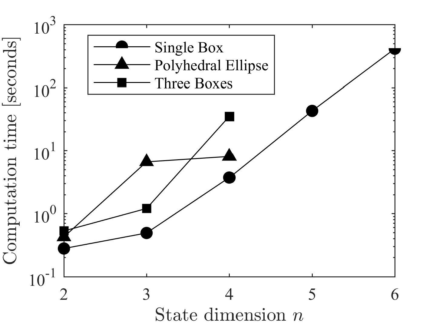
Figure 5: Computation time for $\operatorname{Reach}_{0}^{\flat}(\operatorname{\mathscr{T}}_{N},\operatorname{\mathcal{E}}_{R^{2}})$ computed with a single polyhedral overapproximation of an ellipse using 200 random directions (triangles), $\operatorname{Reach}_{0}^{\flat}(\operatorname{\mathscr{T}}_{N},\operatorname{\mathcal{E}}_{\mathrm{box}})$ computed with a single box centered at the origin (circles), and $\operatorname{Reach}_{0}^{\flat+}(\operatorname{\mathscr{T}}_{N},\operatorname{\mathcal{E}}_{[1,3]})$ with three boxes (squares).

For 2 and 3-dimensional integrators using multiple boxes was still faster than computation using a polyhedral approximation an ellipse, and while disturbance minimal reach set could not be computed for the ellipsoid disturbance set, we were able to simulate up to a 6-dimensional integrator when using a single $n$-d box disturbance. The rise in computation time is predominately caused by the burden of solving the vertex-facet enumeration problem for higher dimensions.

8.3 Application to space-vehicle dynamics

We now consider a more realistic problem, motivated by the rendezvous and docking problem for a pair of space vehicles. The goal is for one spacecraft, referred to as the deputy, to approach and dock to an orbiting satellite, referred to as the chief, while remaining in a predefined line-of-sight cone, in which accurate sensing of the other vehicle is possible. The dynamics are described by the Clohessy-Wiltshire-Hill (CWH) equations [42]

$$\begin{split}\ddot{x}-3\omega x-2\omega\dot{y}=\frac{F_{x}}{m_{d}}\\ \ddot{y}+2\omega\dot{x}=\frac{F_{y}}{m_{d}}\end{split}$$ (70)

The chief is located at the origin, the position of the deputy is $x,y\in\operatorname{\mathbb{R}}$, $\omega=\sqrt{\mu/R_{0}^{3}}$ is the orbital frequency, $\mu$ is the gravitational constant, and $R_{0}$ is the orbital radius of the spacecraft.

We define the state as $z=[x,y,\dot{x},\dot{y}]\in\operatorname{\mathbb{R}}^{4}$ and input as $u=[F_{x},F_{y}]\in\operatorname{\mathcal{U}}\subseteq\operatorname{\mathbb{R}}^{2}$. We discretize the dynamics (70) in time to obtain the discrete-time LTI system,

$$z_{k+1}=Az_{k}+Bu_{k}+w_{k}$$ (71)

with $w_{k}\in\operatorname{\mathbb{R}}^{4}$ a Gaussian i.i.d. disturbance, with $\mathbb{E}[w_{k}]=0$, $\Sigma=\mathbb{E}[w_{k}w_{k}^{\top}]=10^{-4}\times\mbox{diag}(1,1,5\times 10^{-4},5\times 10^{-4})$. The bounded disturbance sets $\operatorname{\mathcal{E}}$ and $\operatorname{\mathcal{O}}$ are origin-centered 4-dimensional boxes obtained with Algorithm 5.

We define the target sets and as in [1]

$$\operatorname{\mathcal{T}}_{N} =\left\{z\in\operatorname{\mathbb{R}}^{4}:|z_{1}|\leq 0.1,-0.1\leq z_{2}\leq 0,\right.$$

$$\hskip 54.06006pt\left.|z_{3}|\leq 0.01,|z_{4}|\leq 0.01\right\}$$ (72)

$$\operatorname{\mathcal{T}}_{i} =\left\{z\in\operatorname{\mathbb{R}}^{4}:|z_{1}|\leq z_{2},|z_{3}|\leq 0.05,|z_{4}|\leq 0.05\right\}$$ (73)

$$\qquad i=1,2,\dots,N-1$$ (74)

$$\operatorname{\mathcal{U}} =[-0.1,0.1]\times[-0.1,0.1].$$ (75)

For a horizon, $N=5$, and a level set, $\alpha=0.8$, $\operatorname{\mathcal{E}}=\{s:s^{\top}\Sigma^{-1}s\leq 6.26\}$, from (57). Figure 6 shows a cross-section at $\dot{x}=\dot{y}=0$ of the resulting underapproximation of the $N=5$ stochastic reach-avoid level set. The computation time for this level set was $14.5$ seconds. Direct comparison of results via dynamic programming is not possible due to dimensionality of the state. However, in [1, Figure 2], a cross-section of $\dot{x}=\dot{y}=0.9$ of the stochastic reach-avoid set was approximated via convex chance-constrained optimization and particle approximation methods. Although these approaches require gridding, they are computationally feasible, unlike dynamic programming. The computation time reported in [1] is approximately $20$ minutes (about $82$ times slower) for just a subset of the state space.

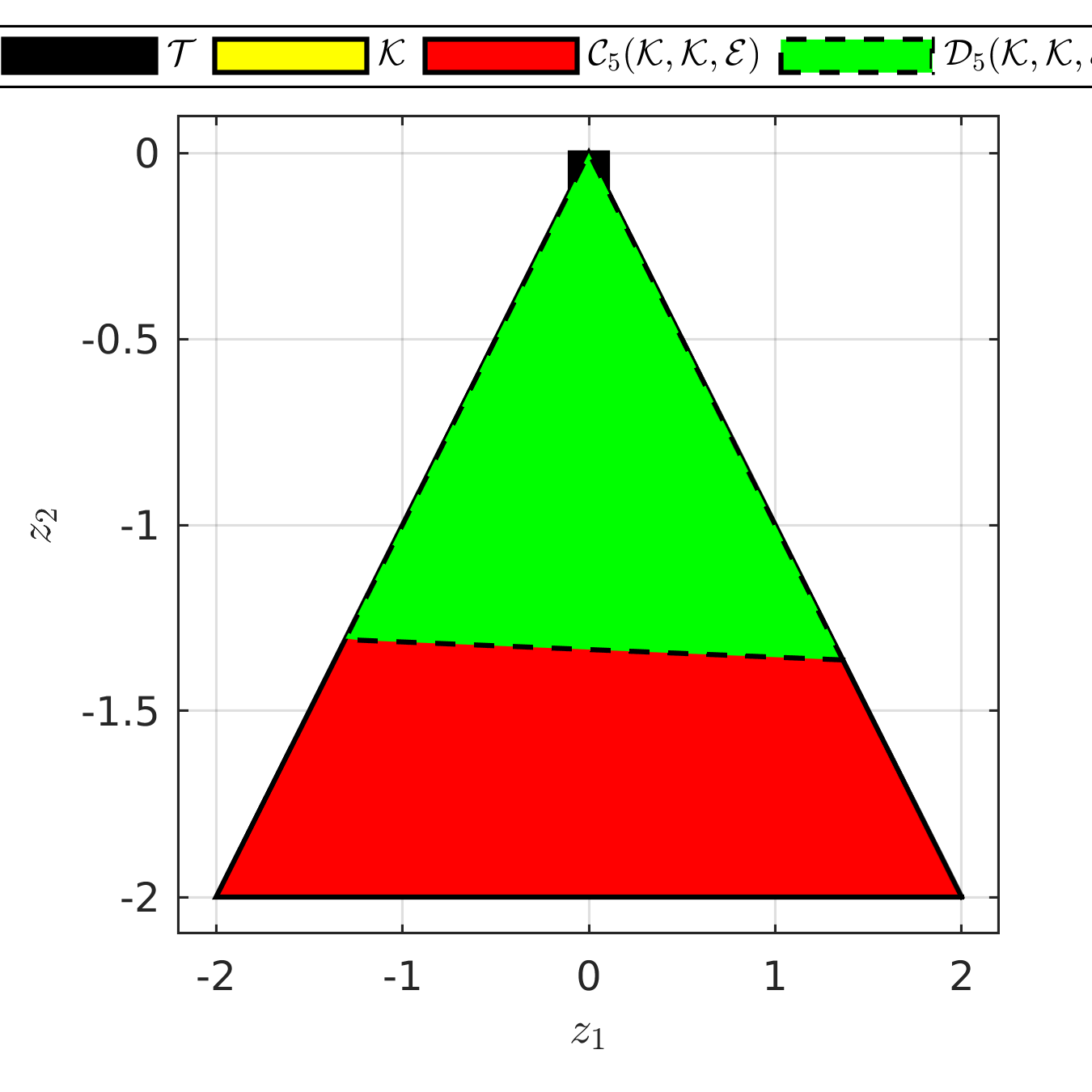
Figure 6: Computation of $\operatorname{Reach}_{0}^{\flat}(\operatorname{\mathscr{T}}_{N},\operatorname{\mathcal{E}})$ and $\operatorname{Reach}_{0}^{\sharp}(\operatorname{\mathscr{T}}_{N},\operatorname{\mathcal{O}})$ for the 4-dimensional CWH spacecraft rendezvous docking problem. Outside of the realm of dynamic programming we are still able to obtain an under and overapproximation of the stochastic reach set using Lagrangian methods.

9 Conclusion

In this work we have demonstrated how Lagrangian recursions can be used to under and overapproximate the stochastic $\alpha$-level reach set of the reachability of the target tube problem. The reachability of a target tube problem was shown to be a more generalized version of both the terminal-time reach-avoid and viability problems. These recursive methods provide substantial gains in computation time when compared to dynamic programming since they do not require on gridding the system, nor are the accuracy of the obtained results related to the spacing of the grid. The Lagrangian results are however, conservative, and while we are able to demonstrate the ability to simulate systems with moderate dimensional size, the current limitations in computational geometry tools limit this growth. In the examples demonstrated, the requirement to solve the vertex-facet enumeration problem is a limiting factor.

In the future, we intend to continue work to allow for Lagrangian methods to provide approximations sets for higher dimensional systems. The use of zonotopes for the overapproximation, for example, may allow for evaluation of higher dimensional systems. Additionally, Lagrangian methods provide fast simulation for a set of states for which existence of a closed-loop feedback controller is guaranteed, however an explicit controller is not provided. We also plan to develop methods that will use the disturbance minimal reach tube, i.e. $[\operatorname{Reach}_{0}^{\flat}(\operatorname{\mathscr{T}}_{N},\operatorname{\mathcal{E}}),\operatorname{Reach}_{1}^{\flat}(\operatorname{\mathscr{T}}_{N},\operatorname{\mathcal{E}}),\dots,\operatorname{Reach}_{N}^{\flat}(\operatorname{\mathscr{T}}_{N},\operatorname{\mathcal{E}})]$ to determine open and closed-loop control strategies that will have the probabilistic guarantees of safety established by the approximation. Controllers can be equivalently found for the disturbance maximal reach tube.

References

- [1] K. Lesser, M. Oishi, and R. S. Erwin, “Stochastic reachability for control of spacecraft relative motion,” December 2013.
- [2] C. Tomlin, I. Mitchell, A. Bayen, and M. Oishi, “Computational techniques for the verification of hybrid systems,” Proc. IEEE, vol. 91, no. 7, pp. 986–1001, 2003.
- [3] S. Summers, M. Kamgarpour, J. Lygeros, and C. Tomlin, “A stochastic reach-avoid problem with random obstacles.” ACM, 2011, pp. 251–260.
- [4] J. N. Maidens, S. Kaynama, I. M. Mitchell, M. M. Oishi, and G. A. Dumont, “Lagrangian methods for approximating the viability kernel in high-dimensional systems,” Automatica, vol. 49, no. 7, pp. 2017–2029, 2013.
- [5] N. Kariotoglou, D. M. Raimondo, S. Summers, and J. Lygeros, “A stochastic reachability framework for autonomous surveillance with pan-tilt-zoom cameras,” 2011, pp. 1411–1416.
- [6] G. Manganini, M. Pirotta, M. Restelli, L. Piroddi, and M. Prandini, “Policy search for the optimal control of Markov Decision Processes: A novel particle-based iterative scheme,” pp. 1–13, 2015.
- [7] S. Summers and J. Lygeros, “Verification of discrete time stochastic hybrid systems: A stochastic reach-avoid decision problem,” Automatica, vol. 46, pp. 1951–1961, September 2010.
- [8] A. Abate, M. Prandini, J. Lygeros, and S. Sastry, “Probabilistic reachability and safety for controlled discrete time stochastic hybrid systems,” Automatica, vol. 44, pp. 2724–2734, October 2008.
- [9] A. Abate, S. Amin, M. Prandini, J. Lygeros, and S. Sastry, “Computational approaches to reachability analysis of stochastic hybrid systems,” 2007, pp. 4–17.
- [10] N. Kariotoglou, S. Summers, T. Summers, M. Kamgarpour, and J. Lygeros, “Approximate dynamic programming for stochastic reachability,” 2013, pp. 584–589.
- [11] N. Kariotoglou, K. Margellos, and J. Lygeros, “On the computational complexity and generalization properties of multi-stage and stage-wise coupled scenario programs,” vol. 94, pp. 63–69, 2016.
- [12] A. P. Vinod and M. M. K. Oishi, “Scalable underapproximation for the stochastic reach-avoid problem for high-dimensional lti systems using fourier transforms,” IEEE Ctrl. Syst. Lett., vol. 1, no. 2, pp. 316–321, October 2017.
- [13] ——, “Scalable underapproximative verification of stochastic LTI systems using convexity and compactness,” in Hybrid Systems: Control and Computation, Porto, Portugal, 2018, (accepted).
- [14] C. Le Geurnic, “Reachability analysis of hybrid systems with linear continuous dynamics,” Ph.D. dissertation, Université Joseph-Fourier, 2009.
- [15] F. Borelli, A. Bemporad, and M. Morari, Predictive Control for Linear and Hybrid Systems. Cambridge University Press, 2017.
- [16] M. Herceg, M. Kvasnica, C. Jones, and M. Morari, “Multi-Parametric Toolbox 3.0,” in Proc. of the European Control Conference, Zürich, Switzerland, July 17–19 2013, pp. 502–510, http://people.ee.ethz.ch/%7Empt/3/.
- [17] A. A. Kurzhanskiy and P. Varaiya, “Ellipsoidal toolbox,” University of California, Berkeley, Tech. Rep., 2006.
- [18] A. Girard, “Reachability of uncertain linear systems using zonotopes,” in Proceedings of the 8th International Conference on Hybrid Systems: Computation and Control, 2005, pp. 291–305.
- [19] M. Althoff, “An introduction to cora 2015,” in Proceedings of the Workshop on Applied Verification for Continuous and Hybrid Systems, 2015.
- [20] S. Bak and P. S. Duggirala, “Hylaa: A tool for computing simulation-equivalent reachability for linear systems,” in Proceedings of the 20th International Conference on Hybrid Systems: Computation and Control, 2017, pp. 173–178.
- [21] C. Le Guernic and A. Girard, “Reachability analysis of linear systems using support functions,” Nonlinear Analysis: Hybrid Systems, vol. 4, no. 2, pp. 250–262, 2010.
- [22] D. P. Bertsekas and I. B. Rhodes, “On the minimax reachability of target sets and target tubes,” Automatica, vol. 7, no. 2, pp. 233–247, 1971.
- [23] E. C. Kerrigan, “Robust constraint satisfaction: Invariant sets and predictive control,” Ph.D. dissertation, University of Cambridge, 2001.
- [24] S. V. Raković, E. C. Kerrigan, D. Q. Mayne, and J. Lygeros, “Reachability analysis of discrete-time systems with disturbances,” vol. 51, no. 4, pp. 546–560, April 2006.
- [25] P. Saint-Pierre, “Approximation of the viability kernel,” Applied Mathematics and Optimization, vol. 29, no. 2, pp. 187–209, March 1994.
- [26] J. D. Gleason, A. Vinod, and M. M. K. Oishi, “Underapproximation of reach-avoid sets for discrete-time stochastic systems via Lagrangian methods,” in Proceedings of the IEEE Conference on Decision and Control, Melbourne, Australia, December 2017.
- [27] S. Kaynama, M. Oishi, I. M. Mitchell, and G. A. Dumont, “The continual reachability set and its computation using maximal reachability techniques,” in 2011 50th IEEE Conference on Decision and Control and European Control Conference, Dec 2011, pp. 6110–6115.
- [28] D. P. Bertsekas and S. E. Shreve, Stochastic Optimal Control: the Discrete Time Case. Academic Press, 1978.
- [29] R. Rockafellar and R. Wets, Variational analysis. Springer Science & Business Media, 2009, vol. 317.
- [30] D. P. Bertsekas, Dynamic Programming and Optimal Control. Vol. 1, 3rd ed. Belmont, Mass: Athena Scientific, 2005.
- [31] S. Boyd and L. Vandenberghe, Convex optimization. Cambridge Univ. Press, 2004.
- [32] H. Benson and G. Boger, “Multiplicative programming problems: analysis and efficient point search heuristic,” Journal of Optimization Theory and Applications, vol. 94, no. 2, pp. 487–510, 1997.
- [33] R. Horst, P. M. Pardalos, and N. Van Thoai, Introduction to global optimization. Springer Science & Business Media, 2000.
- [34] P. Billingsley, Probability and Measure, 3rd ed. New York: Wiley, 1995.
- [35] A. B. Kurzhanski and P. Varaiya, “Ellipsoidal techniques for reachability analysis,” in Hybrid systems: computation and control, 2000, pp. 202–214.
- [36] R. Harman and V. Lacko, “On decompositional algorithms for uniform sampling from n-spheres and n-balls,” Journal of Multivariate Analysis, vol. 101, no. 10, pp. 2297 – 2304, 2010.
- [37] J. D. Gleason, A. P. Vinod, and M. M. K. Oishi, “Improving lagrangian underapproximations of stochastic reach-avoid level sets,” in IEEE Conference on Decision and Control, Miami, Florida, USA, 2018, (submitted).
- [38] M. Althoff and B. H. Krogh, “Zonotope bund les for the efficient compu tation of reachable sets,” in Proceedings of the IEEE Confernce on Decision and Control, Orlando, FL, USA, 2011.
- [39] R. J. Gardner, D. Hug, and W. Weil, “Operations between sets in geometry,” Journal of the European Mathematical Society, vol. 15, no. 6, pp. 2297–2352, 2013.
- [40] C. Le Guernic and A. Girard, “Reachability analysis of hybrid systems using support functions,” in International Conference on Computer Aided Verification. Springer, 2009, pp. 540–554.
- [41] I. Kolmanovsky and E. G. Gilbert, “Theory and computation of disturbance invariant sets for discrete-time linear systems,” Mathematical Problems in Engineering, vol. 4, pp. 317–367, 1998.
- [42] W. Wiesel, Spaceflight Dynamics. New York: McGraw-Hill, 1989.