Constructing energy accounts for WIOD 2016 release

Abstract

Most of today’s products and services are made in global supply chains. As a result a consumption of goods and services in one country is associated with various environmental pressures all over the world due to international trade. Advances in global multi-region input-output models have allowed researchers to draw detailed, international supply-chain connections between production and consumptions activities and associated environmental impacts. Due to a limited data availability there is little evidence about the more recent trends in global energy footprint. In order to expand the analytical potential of the existing WIOD 2016 dataset to wider range of research themes, this paper develops energy accounts and presents the global energy footprint trends for the period 2000-2014.

1 Introduction

Addressing the problem of climate change has moved high up on the governments’ agendas across the world. Effective strategies to reduce country-specific impacts require accurate and reliable environmental statistics. Such statistics should not only account for environmental pressures occurring within the borders of a country but should also allow to consider environmental pressures embodied in imports and exports.

This issue is of particular importance given that most of today’s products and services are no longer produced within a single country and are made in global supply chains. This means that countries import intermediate goods and raw materials, to which they add one or more layers of value and sell the product either for final consumption or for another producer who adds the next layer (Tukker and Dietzenbacher, 2013). Evidence suggest that the average number of border crossings in value chain required for a product of one country to reach the final user in another country is approximately 1.7 (Muradov, 2016).

Normally environmental impacts are calculated following production-based accounting (PBA) method. This method assigns the responsibility of a specific factor (e.g. energy or CO₂) to a country where the impact occurs. Following the rise in international trade and increasing production fragmentation many scholars begun to discuss appropriate ways to measure the responsibility for emissions and question the effects of trade on the environment (Tukker and Dietzenbacher, 2013; Wiedmann and Lenzen, 2018).

One way to account for the factor content embodied in trade is to use the consumption-based accounting (CBA). Significant attention has been devoted to the use of consumption-based accounting principles (also referred to as footprint) in the past few decades. Multi-regional input-output (MRIO) analysis has proved to be an ideal tool for this task. Recently, the availability of global multi-regional input-output databases enabled researchers to draw detailed, global supply-chain connections between production and consumption of goods and services.

Multiple studies have shown that in the developed countries CO₂ and energy content embodied in imports is higher than in exports. In contrast, for the developing countries the opposite is true, i.e., CO₂ and energy embodied in exports is higher than in imports. Between 1995-2011, the share of total global environmental impacts embodied in trade increased from 20% to 29% for energy use and from 19% to 24% for GHG emissions (Wood et al., 2018).

While the MRIO models are a powerful tool for analysing the carbon footprints of countries, their data and computational requirements are often cited as barriers to timely, detailed and robust studies (Andrew et al., 2009). Recent reviews of the main global MRIO initiatives indicate that there are seven global MRIO databases (Owen, 2015). Four of these (Eora, WIOD2013, EXIOBASE, GTAP) databases come with the environmental extensions that permit environmental analyses (e.g., estimation of carbon or energy footprints). However, in some cases, for instance, the WIOD database released in 2016 does not contain environmental extensions.

Monitoring and understanding global impacts associated with trade of goods and services is essential for effective policy measures. Global Databases with environmental extensions are necessary for this task. This study aims to: i) demonstrate how data from the International Energy Agency (IEA) can be used to construct energy accounts that match the WIOD 2016 sectoral classification, ii) present detailed comparison of WIOD2016 and WIOD2013 energy accounts, and iii) analyse global energy production based accounts (PBA) and consumption based accounts (CBA) for the period 2000-2014.

2 Data

2.1 Energy data

Data for this study comes from two sources: i) International Agency (IEA) and ii) World Input-Output Database (WIOD). IEA (2017) is the main source of energy data. Latest IEA 2017 edition provides World Energy balances for 178 countries and regional aggregates over the period 1960-2015 (OECD countries and regions) and 1971-2015 (non-OECD countries and regions). For each year and country, energy balances cover 67 products and 85 flows. For example, a flow " iron & steel" contains data of how much and what energy product (e.g., coal, oil) iron and steel industry used during a specific year. A final data extract from the IEA has the following dimensions:

$$Year\times country\times flow\times product=14\times 44\times 63\times 85$$

It covers a 14 year period from 2000 to 20014, and contains data for 44 countries, 63 energy products and 85 flows.

Table 1: IEA energy balances, exemplified with data for Germany 2014, (Mtoe)

	Energy Product
	product $1$	product $2$	…	product $67$	Total
TPES					306
Production	…	…	…	…	120
Imports	…	…	…	…	246
Exports	…	…	…	…	-49
International marine bunkers	…	…	…	…	-2
International aviation bunkers	…	…	…	…	-8
Stock changes	…	…	…	…	0.3
Transfers					0.7
Statistical differences					0.3
Transformation processes					-74
…	…	…	…	…
Energy industry own use					-16
…	…	…	…	…	…
Total final consumption					216
Industry					55
…	…	…	…	…	…
Transport					55
…	…	…	…	…	…
Other					84
…	…	…	…	…	…
Non-energy use					22

2.2 MRIO data

Multi-regional input-output (MRIO) tables come from World Input Output Database (WIOD), which contains WIOD 2013 release (WIOD13 hereafter) and WIOD 2016 release (WIOD16 hereafter). WIOD13 version is a system of MRIO tables, socioeconomic and environmental accounts (Genty et al., 2012; Timmer et al., 2015, 2016). It covers 35 industries and 41 countries/regions, including 27 EU and 13 other major advanced and emerging economies, plus Rest of the World (ROW) region over the period 1995-2011 (environmental accounts only for 1995-2009).

A more recent WIOD2016 database provides data for 56 industries and 44 countries (28 EU, 15 other major countries and ROW region) for the period from 2000 to 2014 (see table A.1 and table A.2 in Appendix A). It also provides socio-economic accounts, but it lacks environmental accounts.

The two databases overlap over the period from 2000 to 2009. WIOD2016 estimates are compared to WIOD2013 version over this period to test for the accuracy of the WIOD2016 estimates. The aim is to provide estimates that closely resemble those in WIOD2013 so that the two databases could be linked to study the changes in environmental indicators over an extended period: 1995-2014. This is a novel contribution of this paper and could serve the scientific community in many ways.

3 Methodology

This section outlines the allocation procedure of the 85 flows of the IEA energy balances into the corresponding WIOD16 sectors and final demand categories. The allocation procedure have been outlined in previous studies by Genty et al. (2012); Wood et al. (2015); Wiebe and Yamano (2016); Owen et al. (2017). The procedure to obtain energy accounts starting from energy balances involves a series of steps. Each step with examples is explained below.

3.1 IEA Allocation Procedure

3.1.1 Step 1

The IEA energy balances show the supply and the use of energy products by industries and final use categories as in table 1. This data allows to construct two energy extension vectors: one showing energy use by industry and another showing energy supply of different energy products (e.g. coal) by the source sector (e.g., Mining). The two vectors are equivalent in size (energy supply = energy use), but the allocation to industry sectors is different. Among the existing databases GTAP and WIOD provide energy use vectors, Eora provides energy-supply vectors, and EXIOBASE is the only database to provide both energy vectors (Owen et al., 2017). There is little information on the difference between the two vectors and the choice of which energy extension vector to use when largely depends on the question at hand. Owen et al. (2017) show that both energy extensions produce very similar estimates of the overall energy CBA for the UK. However, at a more detailed level, the results address different issues. For instance, the energy-supply vector reveals how dependent the UK is on the domestic energy supply, an issue that is of utmost importance for energy security policy. On the other hand, the energy use vector allows for the attribution of actual energy use to industry sectors, which enables a better understanding of sectoral efficiency gains.

In order to be consistent with WIOD13 energy accounts, this study focuses on the construction of energy use instead of energy supply. The very first step in deriving energy use accounts from the IEA energy balances is to separate the use and the supply of energy products.

Energy use consists of the total final consumption (Industry + transport + Other + Non-energy use); the aviation and marine bunkers; the energy sector own use (with a changed algebraic sign) and transformation processes (with a changed algebraic sign).

3.1.2 Step 2

The next step is to establish a correspondence key linking energy balance items and WIOD16 industries plus households. An example of a binary correspondence matrix is displayed in table . Zero value "0" means no link and "1" represents a link between the IEA flow and WIOD sector(s). The columns containing only one entry represent one-to-one allocation, for example, column $fl2$ is allocated to WIOD16 sector $s56$. The IEA flows that contain multiple entries of "1" represent one-to-many allocation. For instance, the IEA flow $fl1$ is allocated to two WIOD16 sectors $s1$ and $s2$ and flow $fl85$ is split among all WIOD sectors + households.

Table 2: An example of a binary concordance matrix

		IEA energy flow
		$fl1$	$fl2$	…	$fl85$
WIOD16 (56 sectors + households)	$s1$	1	0	…	1
	$s2$	1	0	…	1
	…	…	…	…	…
	$s56$	0	1	…	1
	$hh$	0	0	…	1

3.1.3 Step 3

While one-to-one allocation is a straightforward task one-to-many allocation requires disaggregation of a specific IEA flow among several WIOD16 sectors. The splitting key is the total input in monetary terms from two WIOD16 energy related sectors: “coke and refined petroleum products” ($s10$) and “Electricity, gas, steam and air conditioning supply” ($s24$). For instance, the splitting key to allocate IEA flow $f1$ among two WIOD16 sectors $s1$ and $s2$ is $=[\begin{array}[]{cc}12/16&4/16\end{array}]=[\begin{array}[]{cc}0.75&0.25\end{array}]$ . This means that 75% of IEA energy flow $f1$ is allocated to $s1$ and 25% to $s2$.

Table 3: An example of a splitting key vector (arbitrary numbers)

		WIOD16 ($)
		s1	s2	…	s56	HH
Coke and refined petroleum products	s10	5	1	…	1	3
Electricity, gas, steam and air conditioning supply	s24	7	3	…	0	11
Total	s10+s24	12	4	…	1	14

In a formal way the procedure in step 2 and step 3 can be written as :

$$\mathbf{M=\hat{a}C\widehat{aC}^{-1}}$$ (1)

where $\mathbf{C}$ is a binary concordance matrix, $\mathbf{a}$ is a splitting vector and $\mathbf{M}$ is a mapping matrix between IEA flow and WIOD16 sectors plus households. Using the information from table 3.1.2 and table 3 this can be expressed in more detail as:

$$\underset{}{\mathbf{C}}=\left[\begin{array}[]{ccc}1&0&1\\ 1&0&1\\ 0&1&1\\ 0&0&1\end{array}\right]\text{ }\underset{}{\mathbf{a}}=\left[\begin{array}[]{cccc}12&4&1&14\end{array}\right]$$

this yields:

$$\underset{}{\mathbf{M}}=\left[\begin{array}[]{ccc}0.75&0&0.39\\ 0.25&0&0.13\\ 0&1&0.03\\ 0&0&0.45\end{array}\right]$$

3.1.4 Step 4

The above steps are combined to obtain the use of energy products by WIOD16 sectors and final demand category using the following equation:

$$\mathbf{W16E=E\times M^{*}}$$ (2)

Where $\mathbf{E}$ is the IEA energy use table as explained in Step 1 with dimension 63 x 5355 (63 products x 85 flows). This matrix is obtained by diagonalising the 63x1 vector corresponding to each IEA energy flow and stacking them horizontally.

$\mathbf{M}^{*}$ is a 5355 x 57 energy use allocation matrix it is obtained by modifying $\mathbf{M}$. Every column from $\mathbf{M}$ is transposed and replicated 63 times to match the energy product dimension. $\mathbf{M}^{*}$ shows how much of each energy product (corresponding to each energy flow) is used by each WIOD16 sector plus households.

$\mathbf{W16E}$ is the resulting energy use matrix with a dimension 63x57 representing the use of 63 energy products by 56 WIOD16 industries plus households. The energy product dimension (63) has been further aggregated to match WIOD13 classification of 27 energy products (See Appendix for energy product detail). The final energy matrix is 27x57. The above steps were repeated for all WIOD16 countries except Rest of the World (RoW). For RoW energy use was estimated by taking IEA World energy use and subtracting all energy use by WIOD16 countries.

Table 4: Simplified IEA energy balance table, (arbitrary numbers)

		IEA product
		$pr1$	$pr2$
IEA flow	$fl1$	100	20
	$fl2$	4	2
	$fl2$	15	1

The procedure presented in step 4 can be illustrated using data from step 2 and step 3. One additional piece of information needed for the example is energy balance data i.e. $\mathbf{E}$. An example of energy balance data is given in table 4. It displays the use of a specific energy product (e.g. oil, coal) by a specific flow (e.g. transport). This information is presented in a matrix form as :

$$\underset{}{\mathbf{E}}=\left[\begin{array}[]{cccccc}pr1&0&pr1&0&pr1&0\\ 0&pr2&0&pr2&0&pr2\end{array}\right]=\left[\begin{array}[]{cccccc}100&0&4&0&15&0\\ 0&20&0&2&0&1\end{array}\right]$$

based on sample data from step 3 $\mathbf{M}^{*}$ is:

$$\underset{}{\mathbf{M^{*}}}=\left[\begin{array}[]{cccc}0.75&0.25&0&0\\ 0.75&0.25&0&0\\ 0&0&1&0\\ 0&0&1&0\\ 0.39&0.13&0.03&0.45\\ 0.39&0.13&0.03&0.45\end{array}\right]$$

This matrix shows for $fl1$, 75% of $pr1$ is allocated to $s1$ and 25% to $s2$ and $pr2$ is allocated in the same way. For $fl2$ both $pr1$ and $pr2$ are allocated to $s3$.

Multiplying $\mathbf{E}$ and $\mathbf{M^{*}}$ yields:

$$\underset{}{\mathbf{W16E}}=\left[\begin{array}[]{cccc}80&27&4&6\\ 15&5&2&0.5\end{array}\right]$$

elements in a first row display the use of $pr1$ by the four sectors, the second row show the use of $pr2$. For instance, $s1$ uses 80 units of $pr1$ and 15 units of $pr2$.

3.1.5 Step 5: Accuracy

The accuracy of WIOD16 energy use estimates was evaluated by measuring the difference between WIOD13 energy and WIOD16 energy. Steen-Olsen et al. (2014) have used a similar approach to estimate MRIO aggregation error. The relative error $\varepsilon$ between WIOD13 $(\mathbf{W13})$ and WIOD16 $(\mathbf{W16})$ for a given year $t$ and country $r$ is defined as:

$$\varepsilon_{t}^{r}=\frac{\mathbf{W16}_{t}^{r}-\mathbf{W13}_{t}^{r}}{\mathbf{W13}_{t}^{r}}$$

where $\mathbf{W13}$ and $\mathbf{W16}$ is total energy use (from a production perspective) for WIOD13 and WIOD16 respectively.

3.1.6 Step 6: Calibration

The final step is to calibrate WIOD16 estimates so that they match those of WIOD13 for the year where the two databases overlap, i.e., 2000-2009. It is important to note that while sectoral detail does not match between the two databases energy product detail is the same, i.e. in WIOD13 energy use for a single country is given by $35\times 27$ energy matrix and WIOD16 $56\times 27$, hence the total energy use by energy product is given by $1\times 27$ vector. The calibration was performed in two steps. First, total energy use by product in WIOD16 ($\mathbf{W16E}$) is divided by total product use in WIOD13 ($\mathbf{W13E}$) as:

$$\alpha=(\mathbf{W16E}_{t}^{r}\mathbf{i)^{\prime}}\widehat{\mathbf{W13E}_{t}^{r}\mathbf{i}}^{-1}$$

Where $\mathbf{W16E}$ is $56\times 27$ WIOD16 energy use matrix, $\mathbf{W13E}$ is $35\times 27$ energy use by product, $\mathbf{i}$ is a vector of ones used for summation, $\alpha$is $1\times 27$ vector that shows over/under estimation of a particular energy product. The second step involves adjusting WIOD16 energy accounts as:

$$\mathbf{W16E}^{calibrated}=\widehat{\alpha}\mathbf{W16E}$$

Here it is assumed that under/over estimation of a particular energy product is equally distributed among all sectors. For instance, if coal use in WIOD16 is found to be underestimated by 2% then for every industry that uses coal its consumption is raised by 2%. The calibration strategy is applied for the years where the two datasets overlap, i.e., 2000-2009.

For the period 2010-2014 an additional step was required to calibrate the estimates. It involved extrapolation of under/over estimation data from previous years using a 5-year moving average.

In order to show the scale of adjustments between the two databases, the results are provided for energy use before and after the calibration. While the energy CBA calculations are performed only using the calibrated data.

3.2 Calculation of Energy Footprint

A standard environmentally extended Leontief model is applied to calculate energy footprints for WIOD13 and WIOD16. The basic Leontief model can be expressed as:

$$\mathbf{x}=(\mathbf{I-A})^{-1}\mathbf{Y}=\mathbf{LY}$$

where $\mathbf{x}$ is the vector of output, $\mathbf{A}$ is the matrix of technical coefficients, $\mathbf{Y}$ is the matrix of final demands and $\mathbf{(I-A)^{-1}=L}$ is the total requirement matrix representing interdependencies between industries. The IO model in equation 1 is extended to incorporate energy use as:

$$\mathbf{E}=\mathbf{e^{\prime}L}\mathbf{Y}$$

where $\mathbf{E}$ is the total energy requirements from consumption perspective (CBA) and $\mathbf{e}$ is the direct energy intensity vector representing energy use per unit of output for a given country.s

4 Results

4.1 WIOD16 allocation results

The difference between WIOD16 energy use estimates in comparison with WIOD13 for selected years and the average for the period 2000-2009 are presented in table LABEL:tab:Chapter4_Tbl1. The results indicate that for most countries WIOD16 and WIOD13 results vary between 1 and 4 per cent and in most cases the difference is positive. For the world total, the results are higher on average by 4.1% implying that WIOD16 energy use estimates are on average higher than WIOD13. However, there are also some exceptions, e.g., Denmark, the Netherlands and Germany.

For Denmark, Malta, Belgium and Luxembourg the estimates display greater discrepancies and vary between 10-20%. For Denmark and Luxembourg the results are underestimated and for Malta and Belgium overestimated. For China and Austria WIOD16, energy use estimates are on average 7-9 % larger than WIOD13. For these countries, the results are less accurate (assuming WIOD13 is a correct measure) than for the rest of the sample, but they are precise (i.e. over/underestimation is similar over the years).

Switzerland, Croatia and Norway were not included in the WIOD13 release, and therefore it was not possible to present the estimation error for these countries.

4.2 PBA and CBA results WIOD13 vs WIOD16

WIOD16 energy use estimates were calibrated to match WIOD13 estimates (the procedure explained in step 6). The calibrated energy accounts are labeled as WIOD16C. Data from all three (WIOD13, WIOD16, WIOD16C) energy accounts have been used to calculate PBA and CBA for the period 2000 to 2014 (1995-2009 for WIOD13). To show yearly variations between different estimates the results are displayed for four selected countries (China, Germany, Japan and the US) in figures 1,2,3,4. The two databases overlap from 2000 to 2009, so this period can be used to study the differences between WIOD13 and WIOD16 and WIOD16_C. It is important to note that PBA indicator for WIOD_C and WIOD13 is the same (or very close) due to calibration but CBA can differ, for example, due to a greater sectoral and country detail.

Figure 1 display CBA and PBA results for the USA. PBA results are virtually the same when calculated using WIOD13 and WIOD16. On the other hand, CBA results are larger when using WIOD16 especially during the period 2000-2006. Finally, we can see that energy use has stabilised in the US after 2008 for both PBA and CBA measures. The are no difference between WIOD16C and WIOD16 for the PBA indicator and for CBA the results are when using WIOD16C, but between 2000-2006 they are still higher than WIOD13.

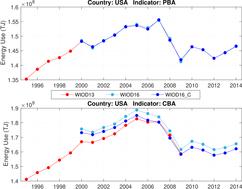
Figure 1: PBA and CBA energy use for the USA, WIOD13 vs WIOD16 and WIOD16C

The same results are displayed for China in figure 2. Here, we can see that WIOD16 results are higher for both PBA and CBA measures, but they follow the same trend as WIOD13. The results for the period after 2009 show that energy use in China continues to increase. WIOD16C results show that with calibrated data CBA measure is almost identical to WIOD13.

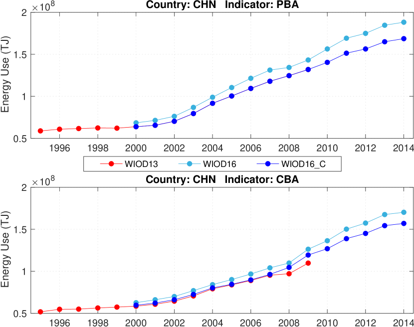
Figure 2: PBA and CBA energy use for China, WIOD13 vs WIOD16 and WIOD16C

The results for Japan are displayed in figure 3. In general, the results for Japan are similar to those of the USA. PBA energy use is virtually the same when calculated using WIOD13 and WIOD16. Whereas, CBA is higher when calculated with WIOD16 than with WIOD13. From 2009 PBA and CBA has declined in Japan. WIODC closely follow WIOD13 for CBA indicator until 2005 after which WIODC gives a lower CBA estimate than WIOD13.

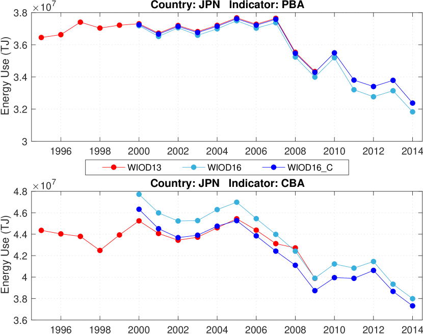
Figure 3: PBA and CBA energy use for the Japan, WIOD13 vs WIOD16 and WIOD16C

The results for Germany displayed in figure 4 show a different story. PBA estimates are virtually the same according to both WIOD13 and WIOD16 calculations. CBA results are different in the sense that WIOD16 display lower values than WIOD13 which is opposite to the deviations seen for the US and Japan. For CBA indicator WIOD16C results are very similar to WIOD16 prior calibration

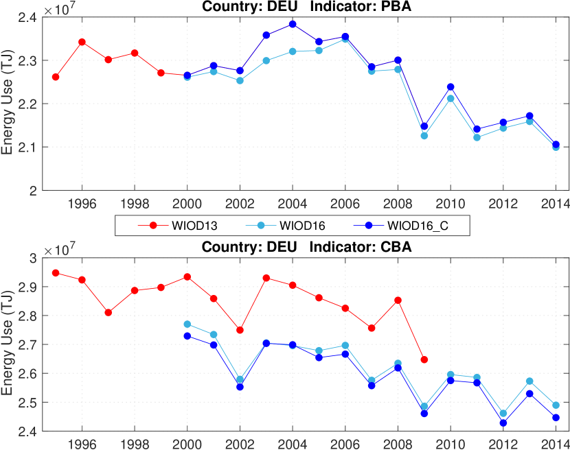
Figure 4: PBA and CBA energy use for the Germany, WIOD13 vs WIOD16 and WIOD16C

4.3 PBA and CBA results for WIOD16

How did energy footprint develop after 2009? and What are the effects of a greater sectoral (56 vs 35) and country detail (44 vs 41) for CBA estimates? To address these questions WIOD16C energy use estimates are presented in table 2 for all countries.

The difference between WIOD13 and WIOD16C energy footprints (CBA) for the period 2000 - 2009 are shown in figure 5. For countries at the top of the figure CBA results are higher when calculated using WIOD16C, and for countries, at the bottom of the graph, the results are lower.

Bulgaria, Malta and Cyprus stand out as outliers in this sample. WIOD16C CBA estimates are on average 30-40% higher than in WIOD13. These countries also display a high degree of variation (0 – 55%) in the results. This implies that in some years the results are quite similar while in others they differ substantially. High degree of variation in the results is also visible for Greece, Slovakia, Estonia, Slovenia, Latvia and Lithuania.

Other countries that have higher CBA in WIOD16C the results fall in the 0-10% range. For instance, for China, Russia, and the US CBA estimates are on average 1.5-3% higher.

Another set of countries including the Netherlands, Romania, Australia, the UK, Taiwan, Japan and Poland do not show significant differences between different databases. The results for these countries are within ±1%.

For the remaining countries at the bottom part of figure 5 CBA results are lower when calculated using WIOD16C. For most countries, the estimates vary between 0-10%. A few notable exceptions are Sweden, Austria, Denmark and Ireland. For these countries, WIOD16C CBA estimates are more than 10% lower compared to WIOD13. The majority of the countries with lower CBA estimates are the EU countries.

The differences between the two databases can occur due to several reasons. First, more detailed sectoral classification (from 35 to 56) can lead to lower estimates if disaggregated sectors (in WIOD16C) have different energy intensities and imports occur predominantly from a sector with a lower intensity. Second, a more detailed country classification can lead to the same outcome if imports come from a country with lower energy intensities than the rest of the world (ROW) aggregate. Finally, the differences in how IO tables and Energy accounts have been compiled also play a role.

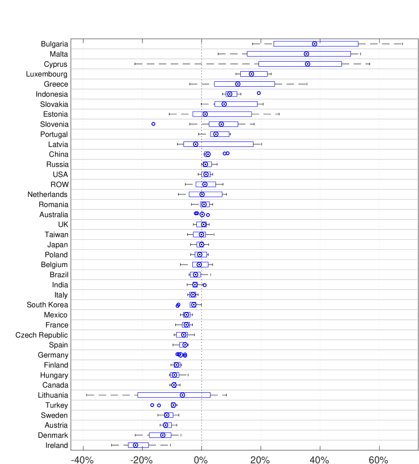
Figure 5: Difference between WIOD13 and WIO16C energy footprint (CBA), 2000-2009

4.3.1 Global Energy footprint 2000-2014

Estimates of CBA and PBA on per capita basis for the years 2000 vs 2014 and the per cent change over the period 2000-2014 are presented in Table LABEL:tab:Chapter4_Tbl2 for all countries covered by WIOD16. The results for both PBA and CBA show substantial variations across countries.

Developed economies, in general, have higher PBA and CBA than developing countries. The USA, Canada and many European countries have PBA and CBA of more than 350 GJ/per capita. In contrast, India has about ten times lower PBA and CBA accounting for roughly 35 GJ/per capita. China had the highest PBA and CBA growth in the sample, both measures increased by 143% between 2000 and 2014, but the levels in 2014 are still less than half of the values for developed countries.

Figure 6 display PBA (solid line) and CBA (dashed line) results over the period 2000-2014 for selected countries and regions. The area between the two lines represents net import (net export) of energy embodied in trade (aka BEET). The solid line above the dashed line implies that a country/region is a net importer of energy and the dashed line above the solid implies that a country is a net exporter of energy.

BRIC and China are net exporters of energy. More energy is embodied in exports of goods and services than in imports. For the USA and the EU28, the result is the opposite. Furthermore, BRIC and China display an increasing PBA and CBA trend, while the USA and the EU28 show stable or declining trend (especially for the EU28).

The difference between PBA and CBA (the shaded area between the two lines) has contracted since about 2008. This implies that the energy content in imports is becoming more balanced over time.

It is also apparent that PBA and CBA are closely correlated; an increase or decline in one measure is followed by a similar change in the other. Such a relationship between the two measures implies that it is just a matter of time until a change experienced in one measure will be replicated by the other. In other words; if PBA declines, CBA will decline too and vice versa. For instance, CBA for BRIC in 2012 was about the same as PBA for BRIC in 2010. For the EU28 and the US, these changes are less visible because the rate of change in the two measures is much slower.

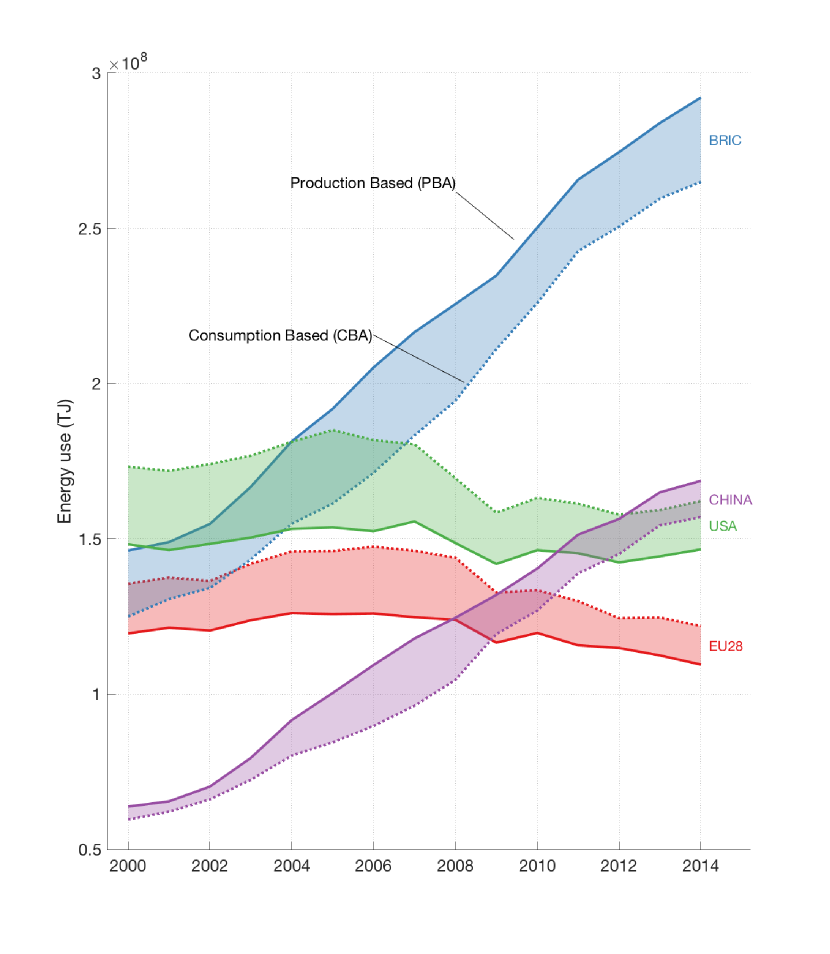
Figure 6: PBA and CBA, 2000-2014 selected countries/regions

5 Discussion and concluding remarks

The aim of this paper has been to construct energy accounts for the WIOD 2016 release and present the main trends in global energy footprints for 2000 – 2014, with a particular focus on the period after 2009, for which the research on energy footprints is lacking.

The newly constructed WIOD16 energy accounts were compared with the existing WIOD13 energy accounts for the period 2000-2009, the period for which the two databases overlap. This exercise shows the accuracy of extended WIOD16 energy accounts. The results show that the difference between WIOD16 and WIOD13 energy accounts for most countries (34 out of 41) are within the 4% range. The differences are mainly due to the allocation procedure. Generally, such differences are not high and in line with known differences between input-output results within the IO community (Moran and Wood, 2014).

To ensure that the two databases are comparable WIOD16 energy accounts were calibrated to match those of WIOD13. As a result, PBA energy is the same in both WIOD13 and WIOD16 energy accounts. However, as shown in figure 5 CBA results differ across countries. For most countries, the differences are within 5% range, and in some extreme cases, the differences range from -20% to +40 %. The negative difference shows by how much CBA is underestimated and the positive result shows how much it is overestimated.

The exact source for these differences is not known, but few possible explanations can be made. First, the differences can occur due to different sectoral and spatial aggregation. WIOD13 is more aggregate than WIOD 2016 both in terms of country and sector detail. The prevailing view is that the finer the level of sector disaggregation the more accurate the results. Su and Ang (2010)use a single-country model to investigate emissions embodied in exports of China and Singapore. They suggest that around 40 sector aggregation is sufficient to capture the majority of $CO_{2}$ emissions embodied in production. Bouwmeester and Oosterhaven (2013) show that for $CO_{2}$ emissions, aggregation errors are on average 2.3% when sectoral detail is reduced from 129 to 59 sectors and about 3.4 % when sectoral detail is reduced from 59 to 10 sectors. The spatial aggregation error is on average 1.4% when aggregating from 43 to 5 regions and 2.4% when aggregating from 5 to 2 regions. However, in most cases the results differ strongly across countries, suggesting that a uniform prescription for the level of sectoral and spatial detail is not possible. Interestingly, the countries that show the largest aggregation error in Bouwmeester and Oosterhaven (2013) study, also appear as having the most significant differences between CBA estimates (figure 5) of this study (e.g., the Baltic countries, Cyprus, Luxembourg, Malta, Greece).

Second, the differences can occur due to different accounting conventions. The WIOD13 IO tables adhere to the 1993 version of System of National Accounts (SNA), and the WIOD2016 release adhere to the 2008 version of SNA. The SNA 2008 version involves two major changes in the recording of international trade statistics. The first concerns changes of goods sent abroad for processing and the second to merchanting (Van De Ven, 2015). In the 1993 SNA goods sent abroad for processing and then returned to the country from where they were dispatched are treated as undergoing an effective change of ownership and recorded as imports and exports Timmer et al. (2016). The 2008 SNA version records transactions on the basis of a change in (economic) ownership which means that goods processed in one country on behalf of another are not recorded as imports and exports even if they physically crossed the borders. These changes have significant consequences for the input-output tables and environmental analysis. Quantitively this leads to lower intermediate consumption, output, import and export estimates. For some countries, the reductions can be quite substantial Aspden (2007). Van Rossum et al. (2014)show that for the Netherlands changing from SNA 1993 to SNA 2008 lead to -8.4% lower estimates for emissions embodied in imports and +12.4% increase in the emission-trade balance. The authors conclude that new SNA 2008 concepts undermine the potential of the environmental input-output analysis.

Intensification of international trade and increasing production fragmentation over the last few decades has made countries more interdependent on one another’s supply of resources. As shown in figure 6 energy content embodied in trade remains high. PBA and CBA measures are highly correlated. This has important implications for the decoupling of energy use from economic growth debate. A prevailing hypothesis suggests that the decoupling seen from the PBA perspective might be a result of production outsourcing. One way to test this hypothesis is to look at the CBA energy use which takes into account imports. Figure 6 shows that the PBA and CBA measures follow a similar trend, and a change in one is closely mirrored by the other. This implies that the decoupling seen in the PBA case will be reassembled by the CBA measure too. That is, PBA and CBA measures will have a similar shape of the so-called Environmental Kuznets curve, only the peak point will differ and the CBA will peak at a higher point.

Appendix A

Table A.1: World Input-Output Database 2016 Country Coverage

No	Name	Code
1	Australia	AUS
2	Austria	AUT
3	Belgium	BEL
4	Bulgaria	BGR
5	Brazil	BRA
6	Canada	CAN
7	Switzerland	CHE
8	People’s Republic of China	CHN
9	Cyprus	CYP
10	Czech Republic	CZE
11	Germany	DEU
12	Denmark	DNK
13	Spain	ESP
14	Estonia	EST
15	Finland	FIN
16	France	FRA
17	United Kingdom	GBR
18	Greece	GRC
19	Croatia	HRV
20	Hungary	HUN
21	Indonesia	IDN
22	India	IND
23	Ireland	IRL
24	Italy	ITA
25	Japan	JPN
26	Republic of Korea	KOR
27	Lithuania	LTU
28	Luxembourg	LUX
29	Latvia	LVA
30	Mexico	MEX
31	Malta	MLT
32	Netherlands	NLD
33	Norway	NOR
34	Poland	POL
35	Portugal	PRT
36	Romania	ROU
37	Russian Federation	RUS
38	Slovakia	SVK
39	Slovenia	SVN
40	Sweden	SWE
41	Turkey	TUR
42	Taiwan	TWN
43	United States	USA
44	Rest of World	ROW

Table A.2: World Input-Output Database 2016 Sectoral Coverage

No	Name	Code
1	Crop and animal production, hunting and related service activities	A01
2	Forestry and logging	A02
3	Fishing and aquaculture	A03
4	Mining and quarrying	B
5	Manufacture of food products, beverages and tobacco products	C10-C12
6	Manufacture of textiles, wearing apparel and leather products	C13-C15
7	Manufacture of wood and of products of wood and cork, except furniture; manufacture of articles of straw and plaiting materials	C16
8	Manufacture of paper and paper products	C17
9	Printing and reproduction of recorded media	C18
10	Manufacture of coke and refined petroleum products	C19
11	Manufacture of chemicals and chemical products	C20
12	Manufacture of basic pharmaceutical products and pharmaceutical preparations	C21
13	Manufacture of rubber and plastic products	C22
14	Manufacture of other non-metallic mineral products	C23
15	Manufacture of basic metals	C24
16	Manufacture of fabricated metal products, except machinery and equipment	C25
17	Manufacture of computer, electronic and optical products	C26
18	Manufacture of electrical equipment	C27
19	Manufacture of machinery and equipment n.e.c.	C28
20	Manufacture of motor vehicles, trailers and semi-trailers	C29
21	Manufacture of other transport equipment	C30
22	Manufacture of furniture; other manufacturing	C31_C32
23	Repair and installation of machinery and equipment	C33
24	Electricity, gas, steam and air conditioning supply	D35
25	Water collection, treatment and supply	E36
26	Sewerage; waste collection, treatment and disposal activities; materials recovery; remediation activities and other waste management services	E37-E39
27	Construction	F
28	Wholesale and retail trade and repair of motor vehicles and motorcycles	G45
29	Wholesale trade, except of motor vehicles and motorcycles	G46
30	Retail trade, except of motor vehicles and motorcycles	G47
31	Land transport and transport via pipelines	H49
32	Water transport	H50
33	Air transport	H51
34	Warehousing and support activities for transportation	H52
35	Postal and courier activities	H53
36	Accommodation and food service activities	I
37	Publishing activities	J58
38	Motion picture, video and television programme production, sound recording and music publishing activities; programming and broadcasting activities	J59_J60
39	Telecommunications	J61
40	Computer programming, consultancy and related activities; information service activities	J62_J63
41	Financial service activities, except insurance and pension funding	K64
42	Insurance, reinsurance and pension funding, except compulsory social security	K65
43	Activities auxiliary to financial services and insurance activities	K66
44	Real estate activities	L68
45	Legal and accounting activities; activities of head offices; management consultancy activities	M69_M70
46	Architectural and engineering activities; technical testing and analysis	M71
47	Scientific research and development	M72
48	Advertising and market research	M73
49	Other professional, scientific and technical activities; veterinary activities	M74_M75
50	Administrative and support service activities	N
51	Public administration and defence; compulsory social security	O84
52	Education	P85
53	Human health and social work activities	Q
54	Other service activities	R_S
55	Activities of households as employers; undifferentiated goods- and services-producing activities of households for own use	T
56	Activities of extraterritorial organizations and bodies	U
57	Households	HH

Table A.3: IEA and WIOD2016 Energy product correspondence

No	WIOD16 energy	IEA energy Product
1	HCOAL	Anthracite; Coking coal; Other bituminous coal; Sub-bituminous coal; Patent fuel
2	BCOAL	Lignite; Coal tar; BKB; Peat; Peat products; Oil shale and oil sands
3	COKE	Coke oven coke; Gas coke
4	CRUDE	Crude oil; Natural gas liquids; Refinery feedstocks; Additives/blending components; Other hydrocarbons
5	DIESEL	Gas/diesel oil excl. biofuels
6	GASOLINE	Motor gasoline excl. biofuels
7	JETFUEL	Aviation gasoline; Gasoline type jet fuel; Kerosene type jet fuel excl. biofuels
8	LFO
9	HFO	Fuel oil
10	NAPHTA	Naphtha
11	OTHPETRO	Refinery gas; Ethane; Liquefied petroleum gases (LPG); Other kerosene; White spirit & SBP; Lubricants; Bitumen; Paraffin waxes; Petroleum coke; Other oil products
12	NATGAS	Natural gas
13	OTHGAS	Gas works gas; Coke oven gas; Blast furnace gas; Other recovered gases
14	WASTE	Industrial waste; Municipal waste (renewable); Municipal waste (non-renewable)
15	BIOGASOL	Biogasoline; Other liquid biofuels
16	BIODIESEL	Biodiesels
17	BIOGAS	Biogases
18	OTHRENEW	Primary solid biofuels; Charcoal
19	ELECTR	Electricity
20	HEATPROD	Elec/heat output from non-specified manufactured gases; Heat output from non-specified combustible fuels; Heat
21	NUCLEAR	Nuclear
22	HYDRO	Hydro
23	GEOTHERM	Geothermal
24	SOLAR	Solar photovoltaics; Solar thermal
25	WIND	Wind
26	OTHSOURC	Tide, wave and ocean; Other sources
27	LOSS

References

- Andrew et al. (2009) Andrew, R., Peters, G. P., and Lennox, J. (2009). Approximation and regional aggregation in Multi-Regional Input-Output Analysis for national carbon footprint accounging. Economic Systems Research, 21(3):311–335.
- Aspden (2007) Aspden, B. C. (2007). The Revision of the 1993 System of National Accounts What does it change ? OECD, 2(2).
- Bouwmeester and Oosterhaven (2013) Bouwmeester, M. C. and Oosterhaven, J. (2013). Specification and Aggregation Errors in Environmentally Extended Input-Output Models. Environmental and Resource Economics, 56(3):307–335.
- Genty et al. (2012) Genty, A., Arto, I., and Neuwahl, F. (2012). Final Database of Environmental Satellite Accounts: Technical Report on Their Compilation. WIOD Deliverable, 4.6:1–69.
- IEA (2017) IEA (2017). World Energy Balances 2017. Technical report, International Energy Agency.
- Moran and Wood (2014) Moran, D. and Wood, R. (2014). Convergence between the Eora, WIOD, EXIOBASE, and OpenEU’s consumption-based carbon accounts. Economic Systems Research, 26(3):245–261.
- Muradov (2016) Muradov, K. (2016). Counting borders in global value chain. In The 24th International Input-Output Conference.
- Owen et al. (2017) Owen, A., Brockway, P., Brand-Correa, L., Bunse, L., Sakai, M., and Barrett, J. (2017). Energy consumption-based accounts: A comparison of results using different energy extension vectors. Applied Energy, 190:464–473.
- Owen (2015) Owen, A. E. (2015). Techniques for evaluating the differences in consumption- based accounts. PhD thesis, The University of Leeds.
- Steen-Olsen et al. (2014) Steen-Olsen, K., Owen, A., Hertwich, E. G., and Lenzen, M. (2014). Effects of sector aggregation on CO2 multipliers in multiregional input-output analyses. Economic Systems Research, 26(3):284–302.
- Su and Ang (2010) Su, B. and Ang, B. (2010). Input-output analysis of CO2 emissions embodied in trade: The effects of spatial aggregation. Ecological Economics, 70(1):10–18.
- Timmer et al. (2015) Timmer, M. P., Dietzenbacher, E., Los, B., Stehrer, R., and de Vries, G. J. (2015). An Illustrated User Guide to the World Input-Output Database: the Case of Global Automotive Production. Review of International Economics, 23(3):575–605.
- Timmer et al. (2016) Timmer, M. P., Los, B., Stehrer, R., and De Vries, G. J. (2016). An Anatomy of the Global Trade Slowdown based on the WIOD 2016 Release.
- Tukker and Dietzenbacher (2013) Tukker, A. and Dietzenbacher, E. (2013). Global multiregional input-output frameworks: an introduction and outlook. Economic Systems Research, 25(1):1–19.
- Van De Ven (2015) Van De Ven, P. (2015). New standards for compiling national accounts: what’s the impact on GDP and other macro-economic indicators? Technical report, OECD STATISTICS BRIEF.
- Van Rossum et al. (2014) Van Rossum, M., Delahaye, R., Edens, B., Schenau, S., Hoekstra, R., and Zult, D. (2014). Do the new SNA 2008 concepts undermine Environmental Input Output Analysis. In Conference paper 22nd International Input-Output Conference, 14-18 July 2014, Lisbon, pages 14–18.
- Wiebe and Yamano (2016) Wiebe, K. S. and Yamano, N. (2016). Estimating CO2 Emissions Embodied in Final Demand and Trade Using the OECD ICIO 2015: Methodology and Results.
- Wiedmann and Lenzen (2018) Wiedmann, T. and Lenzen, M. (2018). Environmental and social footprints of international trade. Nature Geoscience, 11(5):314–321.
- Wood et al. (2015) Wood, R., Stadler, K., Bulavskaya, T., Lutter, S., Giljum, S., de Koning, A., Kuenen, J., Schütz, H., Acosta-Fernández, J., Usubiaga, A., Simas, M., Ivanova, O., Weinzettel, J., Schmidt, J. H., Merciai, S., and Tukker, A. (2015). Global sustainability accounting-developing EXIOBASE for multi-regional footprint analysis. Sustainability, 7(1):138–163.
- Wood et al. (2018) Wood, R., Stadler, K., Simas, M., Bulavskaya, T., Giljum, S., Lutter, S., and Tukker, A. (2018). Growth in Environmental Footprints and Environmental Impacts Embodied in Trade: Resource Efficiency Indicators from EXIOBASE3. Journal of Industrial Ecology.