Fractional Laplacians in bounded domains: Killed, reflected, censored and taboo Lévy flights

Abstract

The fractional Laplacian $(-\Delta)^{\alpha/2}$, $\alpha\in(0,2)$ has many equivalent (albeit formally different) realizations as a nonlocal generator of a family of $\alpha$-stable stochastic processes in $R^{n}$. On the other hand, if the process is to be restricted to a bounded domain, there are many inequivalent proposals for what a boundary-data respecting fractional Laplacian should actually be. This ambiguity holds true not only for each specific choice of the process behavior at the boundary (like e.g. absorbtion, reflection, conditioning or boundary taboos), but extends as well to its particular technical implementation (Dirchlet, Neumann, etc. problems). The inferred jump-type processes are inequivalent as well, differing in their spectral and statistical characteristics, which may strongly influence the ability of the formalism (if uncritically adopted) to provide an unambigous description of real geometrically confined physical systems with disorder. Specifically that refers to their relaxation properties and the near-equilibrium asymptotic behavior. In the present paper we focus on Lévy flight-induced jump-type processes which are constrained to stay forever inside a finite domain. That refers to a concept of taboo processes (imported from Brownian to Lévy - stable contexts), to so-called censored processes and to reflected Lévy flights whose status still remains to be unequivocally settled. As a byproduct of our fractional spectral analysis, with reference to Neumann boundary conditions, we discuss disordered semiconducting heterojunctions as the bounded domain problem.

I Motivation

Brownian motion in a bounded domain is a classic problem with an ample coverage in the literature, specifically concerning the absorbing (Dirichlet) and reflecting (Neumann) boundary data (for the present purpose we disregard other boundary data choices). A coverage concerning their physical relevance is enormous as well schuss ; carlsaw .

Anticipating further discussion, we quite inentionally point out source papers dealing with reflected Brownian motion, grebenkov and exposing at some length the method of eigenfuction expansions for the reflected and other boundary-data problems, grebenkov1 -bickel0 , c.f. also risken . The latter method is as well an indispensable tool in the analysis of spectral properties of fractional Laplacians and related jump-type processes in bounded domains. Its direct link with well developed theory of heat semigroups for jump-type processes (mostly these with absorpion/killing) allows to address the statistics of exits from the domain, like e.g. the first and mean first exit times, large time behavior, stationarity issues, probability of survival and its asymptotic decay, c.f. lorinczi -gar . Compare e.g. also gar1 ; mazzolo (Brownian case) and gaps ; kaleta ; frank (Lévy-stable case), where the role of lowest eigenstates and eigenvalues (thence eigenvalue gaps) of the motion generator has appeared to be vital for the description of decay rates of killed stochastic processes. The spectral data of motion generators are relevant for quantifying long-living processes in a spatial trap (e.g. bounded domain), eventually with an infinite life-time.

Currently, the literature devoted to fractional Laplacians and related jump-type processes is extrememly rich, albeit with no efficient interplay/communication between physics and mathematics-oriented communities. There is a definite prevalence of the very active purely mathematical research on this subject matter. On the other hand, even a concise listing of various real-world applications of the fractional calculus in science and engineering is beyond the ramifications of an introductory section of this paper, see e.g. for example collection - laskin . Viewpoints of applied mathematicians can be consulted in bucur - servadei .

A departure point of the present work is an apparent incompatibility of the implementation of reflecting boundary conditions for Lévy flights in the physics-motivated investigations, Refs. dybiec - denisov , while set against varied (inequivalent) proposals available in the mathematical literature, Refs. bogdan - grubb .

We note that a general theory of censored Lévy processes has been developed bogdan , to handle jump-type processes which are not allowed to jump-out of an open, sufficiently regular set $D\subset R^{n}$ (eventually closed, under suitable precautions, guan ). Within this theory, reflected Lévy-stable processes have been introduced and so-called regional fractional Laplacians were identified as generators of these processes, refl ; guan ; warma . Nonlocal analogs of the Neumann boundary data have been associated with them in suitable ranges of the stability parameter, guan . We point out that other analogs of nonlocal Neumann data, imposed directly on the fractional Laplacian, were proposed as well, dipierro .

The existence problem for jump-type processes with an infinite life-time in a bounded domain, seems to have been left aside in the physics literature (see however Refs. gar1 ; mazzolo in connection with diffusion processes and zaba ; gar for a preliminary discussion of the Cauchy process that is trapped in the interval). To the contrary, permanently trapped Lévy-type processes (diffusion processes like-wise) have their well established place in the mathematical literature.

One category of such processes stems from the analysis of the long-time behavior of the survival probability in the case of absorbing enclosures. One may actually single out appropriately conditioned processes that never leaves the domain once started within. Another category can be related to reflecting boundary data. In contrast to the reflected Brownian motion this issue is conceptually more involved and as yet not free from ambiguities in the context of Lévy-stable processes. Thus, both from physical and applied mathematics points of view, constructing well-posed fractional (Lévy) transport models in bounded domains and keeping under control (the degree and physical relevance of) their possible inequivalence is of vital importance.

In the traditional Brownian lore, while giving meaning to the Laplacian in a bounded domain $D\subset R^{n}$, denoted tentatively $\Delta_{D}$, we must account for various admissible boundary data, that are local i.e. set at the boundary $\partial D$ of an open set $D$. One may try to define a fractional power of the Laplacian by importing its locally defined boundary data on $\partial D$, through so-called spectral definition $(-\Delta_{D})^{\alpha/2}$, bucur -what . This operator is known to be different, servadei , from the outcome of the procedure in which one first executes the fractional power of the Laplacian, and next imposes the boundary data, as embodied in the notation $(-\Delta)^{\alpha/2}_{D}$. In case of absorbing boundaries, in contrast to $(-\Delta_{D})^{\alpha/2}$ where Dirichlet conditions can be imposed locally at the boundary $\partial D$ of $D$, for $(-\Delta)^{\alpha/2}_{D}$ these data need to be imposed as exterior ones i.e. in the whole complement $R^{n}\backslash D$ of $D$.

In passing we note that it is the nonolocality of fractional motion generators (fractional Laplacians) that is the main source of difficulties if the finite-size domain problems are to be considered. In the familiar to physicists lore of Riemann-Liouville fractional derivatives, defined in the Caputo sense, it is known that the divergence problems arise near the domain boundaries. In the study of transport properties of magnetically confined plasmas, negrete , a regularization of the otherwise singular fractional derivative of a general function, has been accomplished by subtracting the boundary terms. A careful handling of such terms appears to be vital in the present research, and allows to make a clear distinction between e.g. absorbing, censored and reflected processes and the corresponding fractional motion generators.

Reflected Brownian motions belong to the bounded domain paradigm, bickel0 ; bickel and the general family of censored Lévy flights (reflected case being included) likewise. If one resorts to the spectral definition of the fractional Laplacian on $D$, Neumann conditions can be imported directly from the Brownian framework and imposed locally.

This is not the case, if censored Lévy processes and regional Laplacians enetr the game. In connection with reflected Lévy flights, a fairly nontrivial problem is to deduce a proper nonlocal analog of the Neumann boundary condition, so that the existence status of the regional generator (and thence of the induced process) can be granted. Even more diffucult issue is to provide a consistent (semi)phenomenological picture of the reflection mechanism, that should underly (or directly follow from) the mathematical procedure. Notwithstanding, Neumann type problems can be obtained in many ways, depending on the kind of ”reinjection” we impose on the outside jumps, barles .

The physically appealing reflection mechanism (a limiting infinite well/trapping interval case of the strongly anharmonic Langevin - Lévy evolution, c.f. Refs. dybiec - denisov , cannot be justified on the basis of the existing mathematical theory of reflected L ́evy processes of Refs. bogdan ; guan ; warma and needs a deepened discussion concerning its meaning and range of validity. On purely mathematical grounds, the resultant asymptotic probability density function can be readily recognized gar as so-called $\alpha$ - harmonic function of the fractional Laplacian $(-\Delta)^{\alpha/2}_{D}$. Here we emphasize that the $\alpha$-harmonic function needs to be defined globally in $R$, albeit may vanish beyond $D$, i.e in $R\backslash D$.

A strictly positive part (restricted exclusively to $D$) of the pertinent function, while normalized on $D$, can be interpreted as a probability density and, according to Ref. denisov , sets a formal explanation of the ”origin of the preferred concentration of flying objects near the boundaries in nonequilibrium systems”.

We note that in the interior of $D$ this pdf rapidly diverges while approaching the boundary, in the whole parameter range $\alpha\in(0,2)$. Such probability accumulation in the vicinity of the boundary barrier has been reported recently in the analysis of the fractional Brownian motion with a reflecting wall wada , albeit only in the superdiffusive regime $\alpha>1$, while a probability depletion close to the barrier has been a characteristic of the subdiffusive regime $\alpha<1$.

Reflecting barriers were seldom seriously addressed by physicists in case of Lévy -type processes, fractional diffusions and continuous time random walks scenarios. On the other hand, their role in the so-called fractional Brownian motion and general anomalous diffusion problems has been analyzed, neel ; metzler ; metzler1 , with observations that are different from the previously outlined ones. As well they remain incongruent with more mathematically oriented (including computer-assisted) research on reflected Lévy flights and fractional diffusion with reflection, meer .

In the present paper, the main body of arguments has its roots in the theory of (nonlocally induced, Lévy-stable) Markov stochastic processes and spectral properties of their (nonlocal as well, fractional) generators. Hence many interesting resarch streamlines which refer to varied realisations of anomalous diffusions (processes with memory,those deriving from the continuous time random walks (CTRW), standard fractional Brownian motion, etc.) are left aside. Nonetheless we mention some source papers, that investigate relaxation properties in the fractional transport that is governed by generalized Langevin equations (GLE), in particular in a finite domain, oliveira ; kinley ; vainstein and specifically wada ; metzler2 in the context of the fractional Brownian motion, where depletion or accretion zones of particles near boundaries have been numerically predicted.

In the latter case metzler a clear specification is given of what pragmatically oriented researchers interpret as a reflection from the boundary (there are different prescriptions that may lead to inequivalent outcomes). The reflection recipe always refers to the trajectory behavior in the vicinity of the boundary. One needs to state clearly how to execute a reflection in the Monte Carlo path-wise simulations, i.e. not to cross the boundary once a jump of a given length would definitely take us away from the trapping enclosure. Compare e.g. our discussion in section VI and a related discussion of reflection conditions in Refs. dybiec -denisov . Neither of these papers addresses the reflection boundary conditions for motion generators per se.

II Varied (in)equivalent faces of the fractional Laplacian.

II.1 Fractional Laplacians in $R^{n}$

In the present paper, up to suitable adjustment of dimensional constants, the free stochastic evolution in $R^{n}$ refers either to the nonnegative motion generator $-\Delta$ (Brownian motion) or $(-\Delta)^{\alpha/2}$ with $0<\alpha<2$ (Lévy-stable motion). One should keep in mind that it is $-(-\Delta)^{\alpha/2}$ which stands for a legitimate fractional relative of the ordinary Laplacian $\Delta$.

It is known that there are many formally different definitions of the fractional Laplacian which actually are equivalent, kwasnicki . For our purposes we shall reproduce three equivalent in $R^{n}$ definitions of the symmetric Lévy stable generator, which nowadays are predominantly employed in the literature (we do not directly refer to the popular notion of a fractional derivative, although formally one can write $(-\Delta)^{\alpha/2}\equiv-\partial^{2}/\partial|x|^{\alpha/2}$, whatever a specific form of $(-\Delta)^{\alpha/2}$ is chosen).

The spatially nonlocal fractional Laplacian has an integral definition (involving a suitable function $f(x)$, with $x\in R^{n}$) in terms of the Cauchy principal value (p.v.), that is valid in space dimensions $n\geq 1$

$$(-\Delta)^{\alpha/2}f(x)=\mathcal{A}_{\alpha,n}\lim\limits_{\varepsilon\to 0^{+}}\int\limits_{{R}^{n}\supset\{|y-x|>\varepsilon\}}\frac{f(x)-f(y)}{|x-y|^{\alpha+n}}dy.$$ (1)

where $dy\equiv d^{n}y$ and the (normalisation) coefficient:

$$\mathcal{A}_{\alpha,n}=\frac{2^{\alpha}\Gamma({\frac{\alpha+n}{2}})}{\pi^{n/2}|\Gamma(-{\frac{\alpha}{2}})|}=\frac{2^{\alpha}\alpha\Gamma({\frac{\alpha+n}{2}})}{{\pi^{n/2}\Gamma(1-\alpha/2})}$$ (2)

Here one needs to employ $\Gamma(1-s)=-s\Gamma(-s)$ for any $s\in(0,1)$. The normalisation coefficient has been adjusted to secure that the integral definition stays in conformity with its Fourier transformed version. The latter actually gives rise to the widely (sometimes uncritically) used Fourier multiplier representation of the fractional Laplacian, kwasnicki ; bucur ; abtangelo ; what ; kwa :

$${\cal{F}}[(-\Delta)^{\alpha/2}f](k)=|k|^{\alpha}{\cal{F}}[f](k).$$ (3)

We recall again, that it is $-(-\Delta)^{\alpha/2}$ which is a fractional analog of the Laplacian $\Delta$.

Another definition, being quite popular in the literature in view of more explicit dependence on the ordinary Laplacian, derives directly from the standard Brownian semigroup $\exp(t\Delta)$ (in passing we note that the Lévy semigroup reads $\exp[-t(-\Delta)^{\alpha/2}]$. The pertinent semigroup is explicitly built into the formula, originally related to the Bochner’s subordination concept, kwasnicki ; kwa ; vondr :

$$(-\Delta)^{\alpha/2}f={\frac{1}{|\Gamma(-{\frac{\alpha}{2}})|}}\,\int_{0}^{\infty}(e^{t\Delta}f-f)t^{-1-\alpha/2}\,dt.$$ (4)

Clearly, given an initial datum $f(x)$, we deal here directly involved a solution of the standard (up to dimensional coefficient) heat equation $f(x,t)=(e^{t\Delta}f$ in the above integral formula.

We note, that based on tools from functional analysis (e.g. the spectral theorem), this definition of the fractional Laplacian extends to fractional powers of more general non-negative operators, than $(-\Delta)$ proper. This point will receive more attention in below.

Remark 1: While computing the singular integral (1), one needs some care if a decomposition into a sum of integrals is involved. An alternative definition

$$(-\Delta)^{\alpha/2}f(x)={\frac{\mathcal{A}_{\alpha,n}}{2}}\int_{R^{n}}\frac{2f(x)-f(x+y)-f(x-y)}{|y|^{n+\alpha}}\,dy,$$ (5)

if employed in suitable function spaces, is by construction free of singularities and does not involve the pertinent decompositions, bucur ; servadei ; abtangelo .

II.2 Fractional Laplacians in a bounded domain.

II.2.1 Restricted (hypersingular) fractional Laplacian

As mentioned before, a domain restriction to a bounded subset $D\subset R^{n}$ is hard, if not impossible, to implement via the Fourier multiplier definition. The reason is an inherent spatial nonlocality of Lévy-stable generators.

We confine attention to the Dirichlet boundary data in a bounded domain. Here one begins from the formal fractional operator definition in $R^{n}$ and restricts its action to suitable functions with support in $D\subset R^{n}$. It is known that the standard Dirichlet restriction $f(x)=0$ for all $x\in\partial D$ is insufficient. One needs to impose the so-called exterior Dirichlet condition: $f(x)=0$ for all $x\in R\backslash D$.

Let us tentatively assume that $f=g$ does not identically vanish in $R^{n}\backslash D$. The formal definition (1) (we use the principal value $p.v.$ abbreviation for the integral) yields:

$$(-\Delta)^{\alpha/2}f(x)=\mathcal{A}_{\alpha,n}p.v.\int_{R^{n}}\frac{f(x)-f(y)}{|x-y|^{\alpha+n}}dy=\mathcal{A}_{\alpha,n}\left[p.v.\int_{D}\frac{f(x)-f(y)}{|x-y|^{\alpha+n}}dy+\int_{R^{n}\backslash D}{\frac{f(x)-g(y)}{|x-y|^{\alpha+n}}}dy\right].$$ (6)

Upon setting $g(x)=0$ for all $x\in R\backslash D$, we arrive at the restricted fractional Laplacian $(-\Delta)^{\alpha/2}_{D}$, whose integral definition is shared with $(-\Delta)^{\alpha/2}$, c.f. Eq. (1), but whose domain is restricted to functions vanishing in $R^{n}\backslash D$. Accordingly, for all $x\in D$ we have

$$(-\Delta)^{\alpha/2}_{D}f(x)=(-\Delta)^{\alpha/2}f(x)=h(x)$$ (7)

where the function $h(x)$ may not have the exterior property of $f(x)$. We point out that there is no restriction upon the the integration volume which is a priori $R^{n}$ and not solely $D\subset R^{n}$. Indeed:

$$(-\Delta)^{\alpha/2}f(x)=\mathcal{A}_{\alpha,n}\left[p.v.\int_{D}\frac{f(x)-f(y)}{|x-y|^{\alpha+n}}dy+f(x)\int_{R^{n}\backslash D}{\frac{dy}{|x-y|^{\alpha+n}}}\right].$$ (8)

so that the exterior $R^{n}\backslash D$ contribution affects the outcome of (7) for all $x\in D$.

In case of sufficiently regular domains, we encounter here a solvable spectral (eigenvalue) problem for the fractional Laplacian in a bounded domain $D$: $(-\Delta)^{\alpha/2}_{D}\phi_{k}(x)=\lambda_{k}\phi_{k}(x)$, $k\geq 1$. This spectral issue has an ample coverage in the literature, and with regard to a detailed analysis of various eigenvalue problems for restricted fractional Laplacians, especially of the fully computable $1D$ case in the interval $(-1,1)=D\subset R$, we mention Refs. kulczycki , duo - mypre , see also kwa .

We note that Eq. (8) can be converted to the form of the hypersingular Fredholm problem, discussed in detail in Refs. zaba0 ; zaba1 ; mypre0 ; mypre . All involved singularities can be properly handled (are removable) and eventually one arrives at the formula, mypre0 :

$$(-\Delta)^{\alpha/2}_{D}f(x)\equiv-{\cal{A}}_{\alpha,n}\int_{\bar{D}}{\frac{f(u)}{|u-x|^{n+\alpha}}}\,du$$ (9)

where $x\in D$ and $D$ is the ultimate integration area. The $R\backslash D$ input, implicit in Eq. (8), has been completely eliminated.

II.2.2 Spectral fractional Laplacian

We first impose the boundary conditions upon the Dirichlet Laplacian in a bounded domain $D$ i. e. at the boundary $\partial D$ of $D$. That is encoded in the notation $\Delta_{\cal{D}}$. Presuming to have in hands its $L^{2}(D)$ spectral solution (employed before in connection with (7)), we introduce a fractional power of the Dirichlet Laplacian $(-\Delta_{\cal{D}})^{\alpha/2}$ as follows:

$$(-\Delta_{\cal{D}})^{\alpha/2}f(x)=\sum_{j=1}^{\infty}\lambda_{j}^{\alpha/2}f_{j}\phi_{j}(x)={\frac{1}{|\Gamma(-{\frac{\alpha}{2}})|}}\,\int_{0}^{\infty}(e^{t\Delta_{\cal{D}}}f-f)t^{-1-\alpha/2}\,dt.$$ (10)

where $f_{j}=\int_{D}f(x)\phi_{j}(x)dx$ and $\phi_{j},j=1,2,...$ form an orthonormal basis system in $L^{2}(D)$: $\int_{D}\phi_{j}(x)\phi_{k}(x)dx=\delta_{jk}$.

We note that the spectral fractional Laplacian $(-\Delta_{\cal{D}})^{\alpha/2}$ and the ordinary Dirichlet Laplacian $\Delta_{\cal{D}}$ share eigenfunctions and their eigenvalues are related as well: $\lambda_{j}\leftrightarrow\lambda_{j}^{\alpha/2}$. The boundary data for $(-\Delta_{\cal{D}})^{\alpha/2}$ are imported from these for $\Delta_{\cal{D}}$.

From the computational (computer-assisted) point of view, this spectral simplicity has been considered as an advantage, compared to other proposals, c.f. vazquez ; teso ; musina .

In contrast to the situation in $R^{n}$, the restricted $(-\Delta)^{\alpha/2}_{D}$ and spectral $(-\Delta_{\cal{D}})^{\alpha/2}$ fractional Laplacians are inequivalent and have entirely different sets of eigenvalues and eigenfunctions. Basic differences between them have been studied in servadei , see also bucur ; abtangelo and duo . An extended study of the intimately related subordinate killed Brownian motion in a domain can be found in Refs. vondr ; vondr1 .

We note one most obvious (and not at all subtle) difference encoded in the very definitions: the boundary data for the restricted fractional Laplacian need to be exterior and set on $R^{n}\backslash D$, while those for the spectral one are set locally at the boundary $\partial D$ of $D$.

Remark 2: In the physics oriented research, the existence of inequivalent fractional Laplacians in case of bounded domains seems to have been overlooked. That led to vigorious discussions luchko ; bayin about the validity of spectral (eigenvalue problems) solutions presented in Refs. laskin0 ; laskin . See also wei for simple standard quantum theory motivated problems, like e.g. the fractional infinite well or harmonic oscillator with mass $m\geq 0$. In particular, Laskin’s spectral solution for the infinite well, as an outcome of his tacit assumptions, coincides precisely with the spectral Laplacian eigenvalue solution $\lambda_{k}^{\alpha/2},\phi_{k}(x),k\geq 1$, given the standard solution $\lambda_{k},\phi_{k}(x),k\geq 1$ of the quantum mechanical infinite well. We point out an explicit usage of the spectral fractional Laplacian in Ref. gitterman , where the fractional process on the interval with absorbing ends has been resolved by means of the spectral affinity with an infnite well problem, gar ; gar1 ; bickel .

Remark 3: Let us mention that solutions of the fractional infinite well problem, together with that of an approximating sequence of deepening fractional finite wells, based on the restricted fractional Laplacian, have been addressed in Refs. zaba ; duo1 ; zaba0 ; zaba1 ; mypre and kwasnicki1 ; kaleta1 ; stos . Moreover, the fractional harmonic oscillator (including the so-called massless version. with the Cauchy generator involved)) has been addressed in a number of papers, gar0 ; zaba0 ; malecki see also durugo for the quartic case.

Remark 4: In Ref. buldyrev the spectral definition of the fractional Laplacian has been comparatively mentioned, prior to the mathematically more refined analysis of Ref. servadei . In fact, a quantitative comparison has been made of the spectral and restricted Dirichlet problems on the interval. Numerical results for various average quantities have been found not to differ substantially. It has been noticed that the restricted Laplacian eigenfunctions are close to the spectral Laplacian eigenfunctions (trigonometric functions) except for the vicinity of the boundaries. An important observation was that the probability decay time rate formulas show up detectable differences. In this connection it is also instructive to record an analogous situation while comparing the pure Brownian case with its he spectral fractional relative.

Remark 5: It is useful to exmplify the differences between the restricted Laplacian and spectral Laplacian outcomes for the interval $(-1,1)$. Namely, according to kwasnicki1 , one arrives at an approximate eigenvalue formula for $n\geq 1$ and $0<\alpha<2$: $\lambda_{n}=\left[{\frac{n\pi}{2}}-{\frac{(2-\alpha)\pi}{8}}\right]^{\alpha}-O\left({\frac{2-\alpha}{n\sqrt{\alpha}}}\right)$. We note that the eignevalues of the ordinary (minus) Laplacian in the interval read $\lambda_{n}=\left[{\frac{n\pi}{2}}\right]^{2}$, $n\geq 1$. Up to dimensional coefficients we have here the familiar quantum mechanical spectrum of the infinite well, set on the interval in question. On the other hand, the spectral fractional well outcome is $\lambda^{\alpha/2}_{n}=\left[{\frac{n\pi}{2}}\right]^{\alpha}$, $n\geq 1$, see also laskin0 ; laskin ; wei .

Remark 6: The ground state function in the restricted case has been proposed in quite complicated analytic form (actrually it is an approximate expression for a ”true” eigenfunction), kwasnicki1 ; stos . Porspective ground state properties were also analyzed in minute detail, with a numemrical assistance, zaba0 ; zaba1 ; duo1 . The available data justify another approximation in terms of a function $\psi(x)=C_{\alpha,\gamma}[(1-x^{2})\cos(\gamma x)]^{\alpha/2}$, where $C_{\alpha,\gamma}$ stands for the $L^{2}(D)$ normalization factor, while $\gamma$ is considered to be the ”best-fit” parameter, allowing to approach quite closely the computer-assisted eigenfunction outcomes, zaba0 . This may be directly compared with the outcome for the spectral case, whose the ground state $cos(\pi x/2)$ is shared with the ordinary Laplacian in the interval.

II.2.3 Regional fractional Laplacian

The regional fractional Laplacian has been introduced in conjunction with the notion of censored symmetric stable processes, bogdan -barles . A censored stable process in an open set $D\subset R^{n}$ is obtained from the symmetric stable process by suppressing its jumps from $D$ to the complement $R^{n}\backslash D$ of $D$, i.e., by restricting its Lévy measure to D. Told otherwise, a censored stable process in an open domain D is a stable process forced to stay inside D. This makes a clear difference with a nuber of proposals to give meaning to Neumann-type conditions, e.g. dipierro ; abtangelo1 , where outside jumps are admitted, albeit with an immediate return (”resurrection”, c.f. bogdan ; pakes ) to the interior of $D$.

Verbally the censorship idea resembles random processes conditioned to stay in a bounded domain forever, gar1 ; mazzolo . However, we point out that the ”censoring” concept is not the same bogdan as that of the (Doob-type) conditioning. Instead, it is intimately related to reflected stable processes in a bounded domain with killing within the domain, or in the least at its boundary, encompassing a class of processes (loosely interpreted as ”reflective”) that do not approach the boundary at all, bogdan ; refl .

In Ref. refl the reflected stable processes in a bounded domain have been investigated, stringent criterions for their admissibility set and their generators identified with regional fractional Laplacians on the closed region $\bar{D}=D\cup\partial D$. According to refl , censored stable processes of Ref. bogdan , in $D$ and for $0<\alpha\leq 1$, are essentially the same as the reflected stable process.

In general, bogdan , if $\alpha\geq 1$, the censored stable process never approaches $\partial D$. If $\alpha>1$, the censored process may have a finite lifetime and may take values at $\partial D$.

Conditions for the existence of the regional Laplacian for all $x\in\bar{D}$, in spatial dimensions higher than one, have been set in Theorem 5.3 of refl . For $1\leq\alpha<2$, the existence of the regional Laplacian for all $x\in\partial D$, is granted if and only if a derivative (this notion is not conventional and is adapted to the nonocal setting) of a each function in the domain in the inward normal direction vanishes, refl ; warma .

For our present purposes we assume $0<\alpha<2$ and $D\subset R^{n}$ being an open set. The regional Laplacian is assumed (a technical assumption employed in the mathematical literature) to act upon functions $f$ on an open set $D$ such that

$$\int_{D}{\frac{|f(x)|}{(1+|x|)^{n+\alpha}}}\,dx<\infty$$ (11)

For such functions $f$, $x\in D$ and $\epsilon>0$, we write (compare e.g. Eqs. (6) - (9))

$$(-\Delta)^{\alpha/2}_{D,Reg}f(x)=\mathcal{A}_{\alpha,n}\lim\limits_{\varepsilon\to 0^{+}}\int\limits_{y\in D\{|y-x|>\varepsilon\}}\frac{f(x)-f(y)}{|x-y|^{\alpha+n}}dy.$$ (12)

provided the limit (actually the Cauchy principal value, p.v.) exists.

Note a subtle difference between the restricted and regional fractional Laplacians. The former is restricted exclusively by the domain property $f(x)=0,x\in R^{n}\backslash D$. The latter is restricted exclusively by demanding the integration variable $y$ of the Lévy measure to be in $D$.

If we impose the Dirichlet domain restriction upon the regional fractional operator ($f(x)=0$ for $x\in R^{n}\backslash D$, $D$ being an open set $D$), we can rewrite Eq. (8) as an identity relating the restricted and regional fractional Laplacians for all $x\in D$, bogdan ; duo ; gar :

$$(-\Delta)^{\alpha/2}f(x)=\left[(-\Delta)^{\alpha/2}_{D,Reg}+\kappa_{D}(x)\right]f(x)$$ (13)

where $\kappa_{D}(x)=\mathcal{A}_{\alpha,n}\int_{R^{n}\backslash D}{|x-y|^{-(n+\alpha)}}dy$ is nonnegative and plays the role of the density of the killing measure, bogdan .

Eqs. (12), (13), actually indicate that the restricted fractional Laplacian can be obtained as a $\kappa_{D}$ perturbation of the regional one (see e.g. bogdan ) and in principle we can move a priority status from the restricted to the regional one. Provided the exterior Dirichlet condition is respected by both operators.

Indeed, while quantifying the random process associated with the generator $(-\Delta)^{\alpha/2}_{D,Reg}+\kappa_{D}(x)$ by invoking the concept of the Feynman-Kac kernel bogdan , one is tempted to view $\kappa_{D}(x)dt$ as a probability of extiction (killing) in the time interval $[t,t+\Delta t]$, and accordingly $\kappa_{D}(x)$ stands for the killing rate.

Proceeding otherwise, we can define the regional Laplacian as a perturbation of the restricted fractional one by the negative (not positive-definite) potential: $(-\Delta)^{\alpha/2}-\kappa_{D}(x)=(-\Delta)^{\alpha/2}_{D,Reg}$. Then however, $\kappa_{D}(x)$ would refer to the resurrection (birth, or creation, bogdan ) rate. One should be aware, that to give meaning to the regional fractional Laplacian, various precautions concerning its domain must be observed to handle potentially dangerous divergent terms ($\kappa_{D}(x)$ being included).

If to replace $D$ in Eq. (12) by $\bar{D}=D\cup\partial D$ then, according to bogdan ; refl , one arrives at the generator of a reflected stable process in $\bar{D}$, c.f. refl , $(-\Delta)^{\alpha/2}_{\bar{D},Reg}f(x)$. Provided suitable conditions (various forms of the Hölder continuity) upon functions in the domain of the nonlocal operator are respected. In particular, in case of $1\leq\alpha<2$ it has been shown that $(-\Delta)^{\alpha/2}_{\bar{D},Reg}f(x)$ exists at a boundary point $x\in∂D$ if and only if the normal inward derivative vanishes: $(\partial f/\partial n)(x)=0$.

We note that an existence of the spectral solution (eigenvalue problem) for the regional Laplacian with (appropriately defined, generally not in an appealing derivative form) Neumann boundary data has been demonstrated in Ref. warma , see e.g. also for the one-dimensional discussion in bogdan ; guan .

Remark 7: To avoid possible misunderstandings and misuse of the concept of killing (and subsequently that of resurrection/birth, pakes ; evans ; evans1 ; durang ), let us recall basic Brownian motion intuitions that underly the the implicit path integral formalism. Namely, operators of the form $\hat{H}=-(1/2)\Delta+V\geq 0$ with $V\geq 0$ give rise to transition kernels of diffusion -type Markovian processes with killing (absorption), whose rate is determined by the value of $V(x)$ at $x\in R$. That interpretation stems from the celebrated Feynman-Kac (path integration) formula, which assigns to $\exp(-\hat{H}t)$ the positive integral kernel

$$\left[\exp(-(t-s)(-{\frac{1}{2}}\Delta+V)\right](y,x)=\int\exp\left[-\int_{s}^{t}V(\omega(\tau))d\tau\right]\,d\mu_{s,y,x,t}(\omega)$$

In terms of Wiener paths that kernel is constructed as a path integral over paths that get killed at a point $X_{t}=x$, with an extinction probability $V(x)dt$ in the time interval$(t,t+dt)$. The killed path is henceforth removed from the ensemble of on-going Wiener paths. The exponential factor $\exp[-\int_{s}^{t}V(\omega(\tau))$ is here responsible for a proper redistribution of Wiener paths, so that the evolution rule

$$\big{(}[\exp(tL)]f\big{)}(x)=\int_{R^{n}}k(x,0;y,t)f(y)dy=E^{x}\big{[}f(X_{t})\big{]}$$

with $-L=-(1/2)\Delta+V$ is well defined as an expectation value of the killed process $X(t)$, but given in terms of Brownian paths $W(t)$ with the Feynman-Kac weight:

$$E^{x}[f(X_{t})]=E^{x}\left[f(W_{t})\exp\left(-\int_{0}^{t}V(W_{\tau})d\tau\right)\right].$$

The resurrection executed with the same $V(x)$ rate would actually refer to another Feynman-Kac weight (note the sign change): $\int\exp[\int_{s}^{t}V(\omega(\tau))d\tau]\,d\mu_{s,y,x,t}(\omega)$, which amounts to the replacement of $V$ by $-V$ in the expression for the motion generator $L$ (as an instructive example one may conceive a replacement of the harmonic oscillator potential by its inverted version, c.f. dual ).

III Relevance versus irrelevance of eigenvalue problems for fractional Laplacians in a bounded domain: Stochastic viewpoint.

III.1 Transition densities

Let us restate our motivations in a more formal lore (our notation is consistent with that in Ref. lorinczi ). Namely, given the (negative-definite) motion generator $L$, we shall consider the (contractive) semigroup evolutions of the form

$$f(x,t)=T_{t}f(x)=\big{(}[\exp(tL)]f\big{)}(x)=\int_{R^{n}}k(x,0;y,t)f(y)dy=E^{x}[f(X_{t})],$$ (14)

where $t\geq 0$. In passing, we have here defined a local expectation value $E^{x}[...]$, interpreted as an average taken at time $t>0$, with respect to the process $X_{t}$ started in $x$ at $t=0$, with values $X_{t}=y\in R^{n}$ that are distributed according to the positive transition (probability) density function $k(x,0;,y,t)$.

We in fact deal with a bit more general transition function $k(x,s;y,t),0\leq s<t$ that is symmetric with respect to $x$ and $y$, and time homogeneous. This justifies the notation $k(x,s;y,t)=k(t-s,x,y)=k(t-s,y,x)$ and subsequently $k(x,0;y,t)=k(t,x,y)=k(t,y,x)$. The ”heat” equation $\partial_{t}f(x,t)=Lf(x,t)$ for $t\geq 0$ is here presumed to follow. We recall, that given a suitable transition function, we recover the semigroup generator via $[Lf](x)=\lim_{t\rightarrow 0}{\frac{1}{t}}\int_{R^{n}}[k(t,x,y)f(y)dy-f(x)]$, in accordance with an (implicit strong continuity) assumption that actually $T_{t}=\exp(Lt)$.

For completeness let us mention that the semigroup property $T_{t}T_{s}=T_{t+s}$, implies the validity of the composition rule $\int_{R^{n}}k((t,x,y)\,k(s,y,z)\,dy=k(t+s,x,z)$. Let $B\subset R^{n}$, a probability that a subset $B$ has been reached by the process $X_{t}$ started in $x\in R^{n}$, after the time lapse $t$, can be inferred from $P[X_{t}\in B|X_{s}=x]=\int_{B}k(t-s,x,y)dy$, $0\leq s<t$, and reads

$$P^{x}(X_{t}\in B)=\int_{B}k(t,x,y)dy=k(t,x,B)$$ (15)

Clearly, $P^{x}(X_{t}\in R^{n})=1$.

In general, for time-homogeneous processes, we have $k(x,s;B,t)=\int_{B}k(t-s,x,y)dy$, $s<t$, hence we can rephrase the Chapman-Kolmogorov relation as follows:

$$\int_{R^{n}}k(x,s;z,u)k(z,u,B,t)dz=k(x,s;B,t)=k(t-s,x,B)=P[X_{t-s}\in B|X_{s}=x],$$ (16)

where $s<u<t$.

III.2 Absorbing boundaries and survival probability

Now, we shall pass to killed Brownian and Lévy-stable motions in a bounded domain. Let us denote $D$ a bounded open set in $R^{n}$. By $T_{t}^{D}$ we denote the semigroup given by the process $X_{t}$ that is killed on exiting $D$. Let $k_{D}(t,x,y)$ be the transition density for $T_{t}^{D}$. Then kulczycki :

$$T_{t}^{D}f(x)=E^{x}[f(X_{t});t<\tau_{D}]=\int_{D}k_{D}(t,x,y)f(y)dy$$ (17)

provided $x\in D$ , $t>0$ and the first exit time $\tau_{D}=\inf\{t\geq 0,X_{t}\notin D\}$ actually stands for the killing time for $X_{t}$.

From the general theory of killed semigroups in a bounded domain there follows that in $L^{2}(D)$ there exists an orthonormal basis of eigenfunctions $\{\phi_{n}\},n=1,2,...$ of $T_{t}^{D}$ and corresponding eigenvalues $\{\lambda_{n},n=1,2,...\}$ satisfying $0<\lambda_{1}<\lambda_{2}\leq\lambda_{3}\leq...$. Accordingly there holds $T_{t}^{D}\phi_{n}(x)=e^{-\lambda_{n}t}\,\phi_{n}(x)$, where $x\in D,t>0$ and we also have:

$$k_{D}(t,x,y)=\sum_{n=1}^{\infty}e^{-\lambda_{n}t}\,\phi_{n}(x)\,\phi_{n}(y)$$ (18)

The eigenvalue $\lambda_{1}$ is non-degenerate (e.g. simple) and the corresponding strictly positive eigenfunction $\phi_{1}$ is often called the ground state function.

For the infinitesimal generator $L_{D}$ of the semigroup we have $L_{D}\phi_{n}(x)=-\lambda_{n}\phi_{n}(x)$ The corresponding ”heat” equation $\partial_{t}f(x,t)=L_{D}f(x,t)$ holds true as well.

It is useful to introduce the notion of the survival probability for the killed random process in a bounded domain $D$. Namely, given $T>0$, the probability that the random motion has not yet been absorbed (killed) and thus survives up to time $T$ is given by

$$P^{x}[\tau>T]=P^{x}[X_{T}\in D]=\int_{D}k_{D}(T,x,y)dy$$ (19)

and is named the survival probability up to time $T$.

Proceeding formally with Eqs. (4) and (5), under suitable integrability and convergence assumptions for the infinite series, one arrives at an asymptotic survival probability decay rule:

$$P^{x}[\tau>T]=\sum_{n=1}^{\infty}e^{-\lambda_{n}T}\,a_{n}\,\phi_{n}(x)\,\Rightarrow\,a_{1}\,e^{-\lambda_{1}T}\,\phi_{1}(x)$$ (20)

where $a_{n}=[\int_{D}\phi_{n}(y)dy]$, $n=1,2,...$. This familiar exponential decay law is characteristic for e.g. the Brownian motion with absorbing boundary data. Its time rate is controlled by the largest eigenvalue $-\lambda_{1}$ of $\Delta_{D}$.

Thus, as far as the asymnptotic properties are concerned, we do not need the fully-fledged spectral solution (e.g. that of the eigenvalue problem for the fractional Laplacian). The lowest eigenvalue and its eigenfunction are what really matters. The degree of accuracy with which we approximate the asymptotic behavior may be improved by not ignoring the second eigenvalue (i.e. the fundamental gap, gaps ). That is also specific to the reflected motion with the lowest eigenvalue zero.

III.3 Conditioned random motions in a bounded domain: taboo processes.

For the absorbing stochastic process with the transition density (17) (thus surviving up to time $T$), we introduce survival probabilities $P^{y}[\tau>T-t]$ and $P^{x}[\tau>T]$, respectively at times $T-t$ and $T$, $0<t<T$. We infer a conditioned stochastic process with the transition density:

$$q_{D}(t,x,y)=k_{D}(t,x,y){\frac{P^{y}[\tau>T-t]}{P^{x}[\tau>T]}},$$ (21)

which by construction survives up to time $T$ and is additionally conditioned to start in $x\in D$ at time $t=0$ and reach the target point $y\in D$, at time $t<T$. An alternative construction of such processes, in the diffusive case, has been described in gar1 .

Given $t<T$, in the large time asymptotic of T, we can invoke (19), and once $T\rightarrow\infty$ limit is executed, Eq. (20) takes the form:

$$q_{D}(t,x,y)\longrightarrow p_{D}(t,x,y)=k_{D}(t,x,y){\frac{\phi_{1}(y)}{\phi_{1}(x)}}\exp(\lambda_{1}t)$$ (22)

We have arrived at the transition probability density $p_{D}(t,xy)$ of the probability conserving process, which never leaves the bounded domain $D$. The latter ”eternal life-time” property is shared with the censored processes of Ref. bogdan , but the pertinent taboo processes (c.f. gar1 ; mazzolo ; pinsky for the origin of the term ”taboo”) appear to form an independent family of random motions.

Its asymptotic (invariant) probability density is $\rho(y)=[\phi_{1}(y)]^{2}$, $\int_{D}\rho(y)\,dy=1$ (that in view of the implicit $L^{2}(D)$ normalization of eigenfunctions $\phi_{n}$).

By employing (19) and the definition $\rho(y)=[\phi_{1}(y)]^{2}$, we readily check the stationarity property. We take $\rho(x)$ as the initial distribution (probability density) of points in which the process is started at time $t=0$). The propagation towards target points, to be reached at time $t>0$, induces a distribution $\rho(y,t)$. Stationarity follows from:

$$\rho(y,t)=\int_{D}\rho(x)p_{D}(t,x,y)dx=\rho(y).$$ (23)

Note that in contrast to $k_{D}(t,x,y)$ the transition probability function $p_{D}(t,x,y)$ is no longer a symmetric function of $x$ and $y$. Compare e.g. in this connection Ref. kaleta .

Remark 8: The semigroup $T_{t}^{D}(\alpha)=\exp(-t(-\Delta)^{\alpha/2}_{D}$, $t\geq 0$ of the stable process killed upon exiting from a bounded set $D$ has an eigenfunction expansion of the form (19). Basically we never have in hands a complete set of eigenvalues and eigenfunctions and likewise we generically do not know a closed analytic form for the semigroup kernel $k_{D}(t,x,y)$, (19). A genuine mathematical achievement has been to establish that when $\alpha\in(0,2)$ and a bounded domain $D$ is a subset of $R^{n}$, then the stable semigroup $T_{t}^{D}(\alpha)$ is intrinsically ultracontractive. This technical (IU) property actually means that for any $t>0$ there exists $c_{t}$ such that for any $x,y\in D$ we have, kulczycki ; kulczycki1 ; grzywny ; chen :

$$k_{D}(t,x,y)\leq c_{t}\,\phi_{1}(x)\phi_{1}(y).$$

Actually we have $k_{D}(t,x,y)=\sum_{1}^{\infty}e^{-\lambda_{n}t}\phi_{n}(x)\phi_{n}(y)$. Accordingly:

$${\frac{k_{D}(t,x,y)}{e^{-\lambda_{1}t}\phi_{1}(x)\phi_{1}(y)}}=1+\sum_{2}^{\infty}e^{-(\lambda_{n}-\lambda_{1})t}\,{\frac{\phi_{n}(x)\phi_{n}(y)}{\phi_{1}(x)\phi_{1}(y)}}.$$

It follows that we have a complete information about the (large time asymptotic) decay of relevant quantities:

$$\lim_{t\to\infty}{\frac{k_{D}(t,x,y)}{e^{-\lambda_{1}t}\phi_{1}(x)\phi_{1}(y)}}=1$$

and (for $t>1$)

$$e^{-(\lambda_{2}-\lambda_{1})t}\leq\sup_{x,y\in D}|{\frac{k_{D}(t,,x,y)}{e^{-\lambda_{1}t}\phi_{1}(x)\phi_{1}(y)}}|\leq C_{\alpha,D}e^{-(\lambda_{2}-\lambda_{1})t}.$$

Thus, what we actually need to investigate the large time regime of Lévy processes in the bounded domain $D$, is to know two lowest eigenvalues $\lambda_{1},\lambda_{2}$ and the ground state eigenfunction $\phi_{1}(x)$ (eventually its shape, banuelos ) of the motion generator, see e.g. also gaps . The existence of conditioned Lévy flights, with a transition density (21) and an invariant probability density $\rho(y)=[\phi_{1}(y)]^{2}$, $\int_{D}\rho(y)\,dy=1$ is here granted.

III.4 Reflected motions in a bounded domain

Reflected random motions in the bounded domain are typically expected to live indefinitely, never leaving the domain, basically with a complete reflection form the boundary. (We cannot a priori exclude a partial reflection, that is accompanied by killing or transmission.)

In case of previously considered motions a boundary may be regarded as either a transfer terminal to the so-called ”cemetry’ (killing/absorption), or as being inaccessible form the interior at all (conditioned processes). In both scenarios, the major technical tool was the eigenfunction expansion (11), where the spectral solution for the Laplacian with the Dirichlet boundary data has been employed. Thus, in principle we should here use the notation $\Delta_{\cal{D}}$, where ${\cal{D}}$ indicates that the Dirichlet boundary data have been imposed at the boundary $\partial D$ of $D\subset R^{n}$.

Reflecting boundaries are related to Neumann boundary data, and therefore we should rather use the notation $\Delta_{\cal{N}}$. In a bounded domain we deal with a spectral (eigenvalue) problem for $\Delta_{\cal{N}}$ with the Neumann data-respecting eigenfunctions and eigenvalues.

The major difference, if compared to the absorbing case is that the eigenvalue zero is admissible and the corresponding eigenfunction $\psi_{0}(x)$ determines an asymptotic (stationary, uniform in $D$) distribution $\rho_{0}(x)=[\psi_{0}(x)]^{2}$, bickel0 ; bickel . In the Brownian context, the rough form of the related transition density looks like:

$$k_{\cal{N}}(t,x,y)={\frac{1}{{\mathrm{vol}}(D)}}+\sum_{n=1}^{\infty}e^{-\kappa_{n}t}\,\psi_{n}(x)\,\psi_{n}(y)$$ (24)

where $\kappa_{n}$ are positive eigenvalues, $\psi_{n}(x)$ respect the Neumann boundary data and $vol(D)$ denotes the volume of $D$ (interval length, surface are etc.). We have $\psi_{0}(x)=1/\sqrt{{\mathrm{vol}}(D)}$.

If one resorts to the spectral definition of the fractional Laplacian in a bounded domain, Neumann conditions are directly imported from these for the standard Laplacian, and thence (see e.g. gitterman ; buldyrev ; bickel the Laplacian eigenvalues $\lambda_{k},k>0$ need to be replaced by $\lambda_{k}^{\alpha/2}$. That is enough to map an eigenfunction expansion of the Laplacian-induced pdf (probability density function) and transition pdf to these appropriate for the fractional case (remebering about the spectral definition of the fractional Laplacian, see also servadei ).

Remark 9: Let us invoke the standard Laplacian in the interval (with an immediate passage to the spectral definition in mind). The case of reflecting boundaries in the interval is specified by Neumann boundary conditions for solutions of the diffusion equation $\partial_{t}f(x)=\Delta_{\cal{N}}f(x)$ in the interval $\bar{D}=[a,b]$. We need to have respected $(\partial_{x}f)(a)=0=(\partial_{x}f)(b)$ at the interval boundaries. The pertinent transition density reads, carlsaw ; bickel :

$$k_{\cal{N}}(t,x,y)={\frac{1}{L}}+{\frac{2}{L}}\sum_{n=1}^{\infty}\cos\left({\frac{n\pi}{L}}(x-a)\right)\cos\left({\frac{n\pi}{L}}(y-a)\right)\exp\left(-{\frac{n^{2}\pi^{2}}{L^{2}}}\,t\right).$$ (25)

The operator $\Delta_{\cal{N}}$ admits the eigenvalue $0$ at the bottom of its spectrum, the corresponding eigenfunction being a constant whose square actually stands for a uniform probability distribution on the interval of length $L$ ($L=2$ in case of $(-1,1)$), to be approached in the asymptotic (large time) limit. Solutions of the diffusion equation with reflection at the boundaries of $D$ can be modeled by setting $p(x,t)=k_{\cal{N}}(t,x,x_{0})$, while remembering that $p(x,0)=\delta(x-x_{0})$. We can as well resort to $c(x,t)=\int_{D}k_{\cal{N}}(t,x,y)c(y)dy$, while keeping in memory that $k(t,x,y)=k(t,y,x)$. Note that all $n\geq 1$ eigenvalues coincide with these of the absorbing case, gitterman . The eigenvalues of the spectral fractional operator for $n>0$ would read $\lambda_{n}^{\alpha/2}=(n^{2}\pi^{2}/4)^{\alpha/2}=(n\pi/2)^{\alpha}$. For comparison we reproduce a rough analytic approximation of the restricted Laplacian eigenvalues $\left[{\frac{n\pi}{2}}-{\frac{(2-\alpha)\pi}{8}}\right]^{\alpha}$, kwasnicki1 , see also mypre for an extended list of numerically generated sharp eigenvalues.

IV Spectral properties of the regional fractional Laplacian.

All derivations and mathematically advanced demonstrations of the existence of regional fractional Laplacianas and their link with (whatever that actually means) reflected Lévy flights and general censored processes, involve subtleties concerning the behavior of functions in their domain, in the vicinity and at the boundaries. Attempts to reconcile a semi-phenomenologically prescribed boundary behavior of censored stochastic processes with the notion of (i) regional fractional Laplacian and (ii) any conceivable forms of Neumann boundary data, lead to inequivalent outcomes. That refers as well to the exoploitation of Sobolev spaces instead of the more familiar for physicists $L^{2}(D)$ Hilbert spaces, warma ; guide . Other subtleties, like an issue of the Hölder continuity up to the boundary, need to be kept under control as well.

All that blurs or even hampers any pragmatic approach aiming at the deduction of approximate (if not sharp) eigenvalues, functional shapes of eigenfunctions, related (approximate) probability distributions and estimates of probability killing rates or decay rates towards equilibrium, if regional fractional Laplacians are interpreted as primary theoretical constructs, instead of the restricted ones.

It is our purpose to follow the pragmatic routine, tested before in our investigation of fractional Laplacians with exterior Dirichlet boundary conditions, zaba0 ; zaba1 ; mypre . We point out the existence of alternative computation routines (based on a direct discretization of fractional Laplacians), duo1 ; duo2 ; pezzo . It is advantageous that we can directly compare our results with these of Ref. duo for the regional Laplacian with the (exterior) Dirichlet boundary data. THis test of a comparative validity of two different computation methods gived support to our subsequent analysis of the full-fledged spectral problem with no Dirichlet restriction, resulting in the implicit relecting boundary conditions.

It is worthwhile to note that the main body of the mathematical research refers to space dimensionalities $d\geq 2$. One should keep in mind, in the least for comparative purposes, that the one-dimensional case (being of interest for us in below) differs form higher dimensional ones in a number of technical points. Notwithstanding the one dimensional case has an advantage of computability and allows for a deeper insight into the properties of motion generators and processes, specifically into an issue of potentially dangerous divergencies.

IV.1 Restricted versus regional fractional Laplacian

We depart from the formal definition (11)-(13) of the regional fractional Laplacian and following gar ; duo concentrate on the one-dimensional spectral problem in the interval. The latter topic, for the Dirichlet fractional Laplacians, has been addressed before in a number of papers in the whole stability parameter range $0<\alpha<2$ and in more detail, for the distinguished $\alpha=1$ value (Cauchy process and motion generator) in Refs. dybiec ; dybiec1 ; dubkov ; denisov , zaba ; zaba0 ; zaba1 ; duo1 ; mypre and kwasnicki ; malecki .

We consider the regional fractional Laplacian (see, e.g. Ref. refl ) acting on the closed interval (including the endpoints) $-1\leq x\leq 1$. To make clear the difference between the regional and ordinary fractional Laplacians, we begin with the fractional Laplacian on the whole real axis. We have, mypre :

$$(-\Delta)^{\alpha/2}\psi(x)=-A_{\alpha}\int_{-\infty}^{\infty}\frac{\psi(u)-\psi(x)}{|u-x|^{1+\alpha}}du,\ A_{\alpha}=\frac{1}{\pi}\Gamma(1+\alpha)\sin\frac{\pi\alpha}{2}.$$ (26)

Since we assume the exterior Dirichlet condition $\psi(u)=0$ for $R\backslash(-1,1)$ (c.f. (8), (9)), the division of the integral into separate contributions from within and ouside the interval

$$(-\Delta)^{\alpha/2}\psi(x)=-A_{\alpha}\int_{-\infty}^{\infty}\frac{\psi(u)-\psi(x)}{|u-x|^{1+\alpha}}du=-A_{\alpha}\left[\int_{-\infty}^{-1}+\int_{-1}^{1}+\int_{1}^{\infty}\right]\frac{\psi(u)-\psi(x)}{|u-x|^{1+\alpha}}du.$$ (27)

implies:

$$(-\Delta)^{\alpha/2}\psi(x)=-A_{\alpha}\left[-\psi(x)\int_{-\infty}^{-1}\frac{du}{|u-x|^{1+\alpha}}+\int_{-1}^{1}\frac{\psi(u)}{|u-x|^{1+\alpha}}du-\psi(x)\int_{-1}^{1}\frac{du}{|u-x|^{1+\alpha}}-\psi(x)\int_{1}^{\infty}\frac{du}{|u-x|^{1+\alpha}}\right]\equiv$$

$$\equiv-A_{\alpha}\left[\int_{-1}^{1}\frac{\psi(u)}{|u-x|^{1+\alpha}}du-\psi(x)\int_{-\infty}^{\infty}\frac{du}{|u-x|^{1+\alpha}}\right]\equiv-A_{\alpha}\int_{-1}^{1}\frac{\psi(u)du}{|u-x|^{1+\alpha}}+\Delta I_{1D}.$$ (28)

Formally, the integral $\Delta I_{1D}$ in (28) indentically vanishes

$$\Delta I_{1D}=-\frac{A_{\alpha}\psi(x)}{\alpha}\left[\frac{1}{|u-x|^{\alpha}}\right]_{-\infty}^{\infty}=0$$ (29)

for all $0<\alpha<2$. This implies that the eigenvalue problem for the operator $|\Delta|^{\alpha/2}$ in the interval (i.e. actually the restricted fractional Laplacian $(-\Delta)^{\alpha/2}_{D}$ of Eq. (9)) is defined by the equation

$$(-\Delta)^{\alpha/2}\psi(x)=-A_{\alpha}\int_{-1}^{1}\frac{\psi(u)du}{|u-x|^{1+\alpha}}=E\psi(x).$$ (30)

The emergent spectrum is discrete $E\equiv E_{n}$, $n=1,2...$, non-degenerate and positive $E_{n}>0$, see e.g. kulczycki ; mypre0 ; mypre and references therein.

The regional fractional Laplacian is defined similarly to Eq. (26) but directly in the interval $D=[-1,1]$ (that refers to the admitted integration area as well), i.e.

$$(-\Delta)^{\alpha/2}_{D,reg}\psi(x)=-A_{\alpha}\int_{-1}^{1}\frac{\psi(u)-\psi(x)}{|u-x|^{1+\alpha}}du=-A_{\alpha}\left[\int_{-1}^{1}\frac{\psi(u)du}{|u-x|^{1+\alpha}}-\psi(x)\int_{-1}^{1}\frac{du}{|u-x|^{1+\alpha}}\right].$$ (31)

We can readily evaluate the integral:

$$\int_{-1}^{1}\frac{du}{|u-x|^{1+\alpha}}=-\frac{1}{\alpha}\frac{1}{(1-x^{2})^{\alpha}}\bigg{[}(1-x)^{\alpha}+(1+x)^{\alpha}\bigg{]}=-{\frac{1}{A_{\alpha}}}\kappa_{D}^{\alpha}(x)$$ (32)

where $D=[-1,1]$ and we meet essentialy the same $\kappa_{D}(x)$ that has emerged in the formula (13), see also Eq. 2.13 in Ref. duo . We emphasize that apart from a difference in the integration volumes for the involved integrals (13) and (32), the outcome of integrations is the same, see e.g. also mypre ). We note a familiar mypre outcome $2/(x^{2}-1)$ for $\alpha=1$.

We thus arrive at the following spectral problem for the regional fractional Laplacian in $D=[-1,1]$:

$$-A_{\alpha}\int_{-1}^{1}\frac{\psi(u)du}{|u-x|^{1+\alpha}}-\frac{A_{\alpha}\psi(x)}{\alpha}\frac{(1-x)^{\alpha}+(1+x)^{\alpha}}{(1-x^{2})^{\alpha}}=E\psi(x).$$ (33)

In short that reads

$$(-\Delta)^{\alpha/2}_{D,Reg}\psi(x)=(-\Delta)^{\alpha/2}\psi(x)-\kappa_{D}^{\alpha}(x)\psi(x)=E\psi(x)$$ (34)

with the persuasive interpretation of $(-\Delta)^{\alpha/2}_{D,Reg}\psi(x)$ as the additive perturbation of $|\Delta|^{\alpha/2}$ by the negative-definite potential $-\kappa_{D}^{\alpha}(x)$. The latter is an inverted version (c.f. dual ) of the attractive singular (c.f. diaz ) potential $\kappa_{D}^{\alpha}(x)$. Its functional shape (the coefficient $A_{\alpha}$ has been skipped) for different values of $\alpha$ is reported in Fig.1.

In passing we note that a concept of resurrected (after killing) Markov processes has been associated with so interpreted random noise generator $(-\Delta)^{\alpha/2}_{D,Reg}\psi(x)$, see e.g. bogdan and pakes .

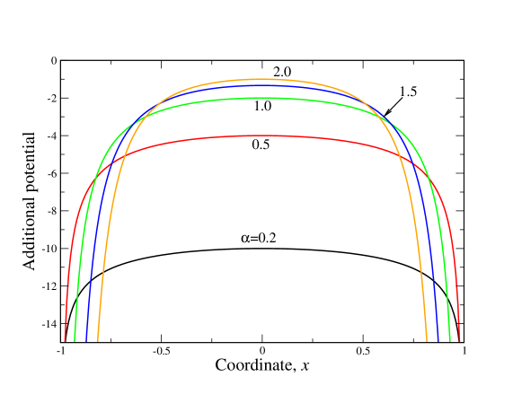
Figure 1: The negative-definite singular potential (32) in the spectral problem for the regional fractional Laplacian for various values of $\alpha$.

IV.2 Regional fractional Laplacian in $L^{2}(D),D=[-1,1]$. Trigonometric base with Dirichlet boundary conditions.

We do not know of any methods towards an analytic solution of the pertinent eigenvalue problem and therefore we reiterate to numerically-assisted arguments, where an explicit diagonalization of Eq. (33) in the $L^{2}(D)$ trigonometric basis can be performed. To this end we shall use the same ”even-odd” base (and the computation method) as that in Ref. mypre . For any function $\psi_{\alpha}(x)$, that may possibly be a solution to the eigenvalue problem, we have the folowing expansions in the trigonometric basis of $L^{2}(D),D=[-1,1]$:

$$\psi_{\alpha e}(x)=\sum_{k=0}^{\infty}a_{k\alpha}\cos\frac{(2k+1)\pi x}{2},\ \psi_{\alpha o}(x)=\sum_{k=1}^{\infty}b_{k\alpha}\sin k\pi x.$$ (35)

So defined would-be basis functions (35) satisfy the Dirichlet boundary conditions $\psi_{\alpha e,o}(\pm 1)=0$. The behavior of the derivative $d\psi(x=\pm 1)/dx$ is immaterial.

Passing to the matrix representation of the eigenvalue problem, for the even subspace we have

$$\sum_{k=0}^{\infty}a_{k}(\gamma_{ki\alpha}+\beta_{ki\alpha})=Ea_{i\alpha}.$$ (36)

Explicitly, the matrix to be diagonalized has the form (we suppress an index $\alpha$ for a moment)

$$\hat{A}_{even}=\left(\begin{array}[]{cccc}\gamma_{00}+\beta_{00}&\gamma_{10}+\beta_{10}&\cdots&\gamma_{n0}+\beta_{n0}\\ \gamma_{10}+\beta_{10}&\gamma_{11}+\beta_{11}&\cdots&\gamma_{n1}+\beta_{n1}\\ \vdots&\cdots&\cdots&\vdots\\ \gamma_{n0}+\beta_{n0}&\gamma_{n1}+\beta_{n1}&\cdots&\gamma_{nn}+\beta_{nn}\end{array}\right),$$ (37)

where $\gamma_{ik}\equiv\gamma_{ki}$ are ”old” mypre matrix elements coming from Eq. (30) (or first term in left hand side of Eq. (33)):

$$\gamma_{ik\alpha}=\int_{-1}^{1}f_{k\alpha}(x)\cos\frac{(2i+1)\pi x}{2}dx,$$ (38)

where $f_{k\alpha}(x)$ are defined by Eq. (16) of Ref. mypre .

At the same time, $\beta_{ki}$ are ”new” matrix elements coming from the second term in the left-hand side of (33), i.e. from the additive negative-definite potential (32):

$$\beta_{ik\alpha}=-\frac{A_{\alpha}}{\alpha}\int_{-1}^{1}\cos\frac{(2i+1)\pi x}{2}\cos\frac{(2k+1)\pi x}{2}\ \frac{(1-x)^{\alpha}+(1+x)^{\alpha}}{(1-x^{2})^{\alpha}}dx.$$ (39)

The integrals for $\beta_{ik1}$ ($\alpha=1$) can be calculated explicitly

$$\beta_{ik1}=\frac{1}{\pi}\Bigg{\{}(-1)^{k-i}{\mathrm{Ci}}[2\pi(1+k+i)]+(-1)^{k+i+1}{\mathrm{Ci}}[2\pi(k-i)]+(-1)^{k+i+1}\ln\frac{1+k+i}{k-i}\Bigg{\}}.$$ (40)

Diagonal elements have the form

$$\beta_{ii1}=\frac{1}{\pi}\Big{\{}-\gamma+{\mathrm{Ci}}[2\pi(1+2i)]-\ln[2\pi(1+2i)]\Big{\}},\ \gamma=0.577216...$$ (41)

Here Ci$(x)$ is cosine integral function abr . Analogously one proceeds with $\gamma_{ik1}$, which can be analytically computed as well, mypre .

For the odd subspace we have

$$\sum_{k=0}^{\infty}b_{k}(\eta_{ki\alpha}+\zeta_{ki\alpha})=Eb_{i\alpha},$$ (42)

where $\eta_{ki\alpha}$ is given by Eq. (35) of Ref. mypre and

$$\zeta_{ik\alpha}=-\frac{A_{\alpha}}{\alpha}\int_{-1}^{1}\sin k\pi x\sin i\pi x\ \frac{(1-x)^{\alpha}+(1+x)^{\alpha}}{(1-x^{2})^{\alpha}}dx.$$ (43)

For concretness, we reproduce a computation outcome in the special (Cauchy) case $\alpha=1$:

$$\zeta_{ik1}=\frac{1}{\pi}\Bigg{\{}(-1)^{k-i}{\mathrm{Ci}}[2\pi(k+i)]+(-1)^{k+i+1}{\mathrm{Ci}}[2\pi(k-i)]+(-1)^{k+i+1}\ln\frac{k+i}{k-i}\Bigg{\}},$$ (44)

$$\zeta_{ii1}=\frac{1}{\pi}\Big{\{}-\gamma+{\mathrm{Ci}}[4i\pi]-\ln[4i\pi]\Big{\}}.$$ (45)

For $\alpha\neq 1$ the same arguments are valid and can be safely reproduced step by step. The only difference is that matrix elements need to be calculated numerically. To obtain the results at the reasonable time cost, we use smaller-sized matrices, around 50x50. This gives access to two decimal places for (lowest) eigenvalues and a fairly good approximation of the corresponding eigenfunctions.

Six lowest eigenvalues for the equation (33) are reported in Table I, for each of the stability indices $\alpha=0.5$, $1.0$ and $1.5$. Quite good coincidence is seen with the spectral data reported in Table 1 of Ref. duo (obtained by an alternative fractional Laplacian discretization method). Since our main purpose has been to test the computation method of mypre0 ; mypre against an alternative proposal of Refs. duo ; duo1 , we refrain from a comparative listing of other eigenvalues and other $\alpha$ choices, see however duo .

$i$	1	2	3	4	5	6
$\alpha=0.5$	0.0048	0.4495	0.8724	1.2189	1.5041	1.7809
$\alpha=0.5$ duo	0.0038	0.4593	0.8626	1.2091	1.5149	1.7911
$\alpha=1.0$	0.1177	1.1926	2.5888	4.0147	5.5328	7.0077
$\alpha=1.0$ duo	0.1135	1.2026	2.5760	4.0292	5.5171	7.0245
$\alpha=1.5$	0.8059	3.6475	7.7541	12.816	18.676	25.230
$\alpha=1.5$ duo	0.8088	3.6509	7.7500	12.811	18.670	25.235

Table 1: Table of 6 lowest eigenvalues of the regional fractional Laplacian for $\alpha=0.5$, 1 and 1.5 calculated for the 2000x2000 matrix, composed with repect to the trigonometric base with Dirichlet boundary conditions. Energy levels are numbered according to standard convention: the lowest (ground) state is labeled by $n=1$ (even state with $k=0$), $n=2$ corresponds to lowest odd state with $k=1$, $n=3$ corresponds to even state with $k=2$ etc. The corresponding eigenvalues from Ref. duo are listed for comparison.

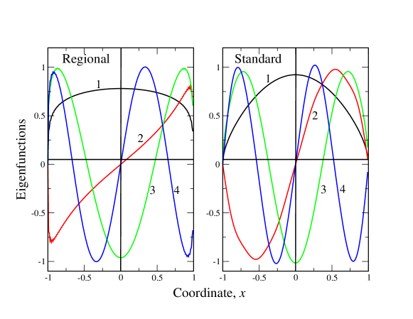
Figure 2: Comparison between four lowest eigenfunctions of the regional (left panel) and restricted (right panel) fractional Laplacians for $\alpha=1$. Eigenstate labels $n=1,2,3,4$ are indicated.

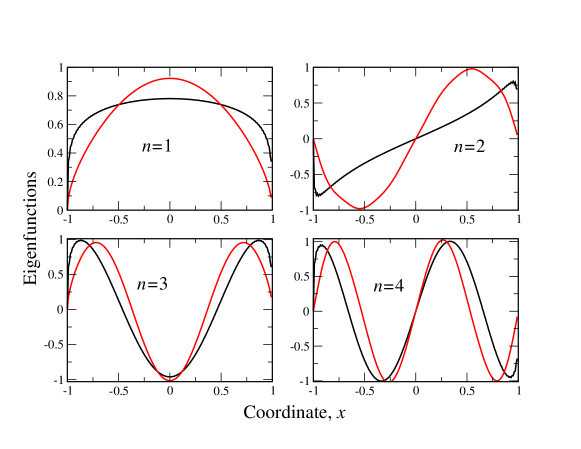
Figure 3: Comparison of first four eigenfunctions of regional and restricted fractional Laplacians, while displayed in pairs corresponding to $n=1,2,3,4$. Black curves refer to the regional Laplacian, red curves to the restricted one; $\alpha=1$.

Four lowest eigenfunctions for $\alpha=1$ are reported in Fig. 2. It is seen (compare e.g. left and right panels of Fig. 2) that the eigenfunctions for regional and standard fractional Laplacians are qualitatively similar with one exception. Namely, those for regional operator show up much sharper decay as $x\to\pm 1$ and their derivatives diverge to infinity as the boundary points are appproached.

More detailed comparative display of Fig. 3 gives further support to our statement about the sharp decay (steep decent down to zero) of the regional fractional Laplacian eigenfunctions, while set against these for the restricted one. Comparing Eqs. (30) with (33), we realize that the milder decay in the restricted case is a consequence of a strong repulsion (scattering) from the boundaries, that is encoded in the functional form of the (inverted) singular potential (32) in the eigenvalue problem of the form (13).

We note that our results are consistent with independent findings of Ref. duo (that refers as well to a different computation method). C.f. Fig. 7 therein, where the first and second eigenfunctions of the restricted and regional fractional Laplacian were compared. Additionally these for the spectral fractional Laplacian have been depicted.

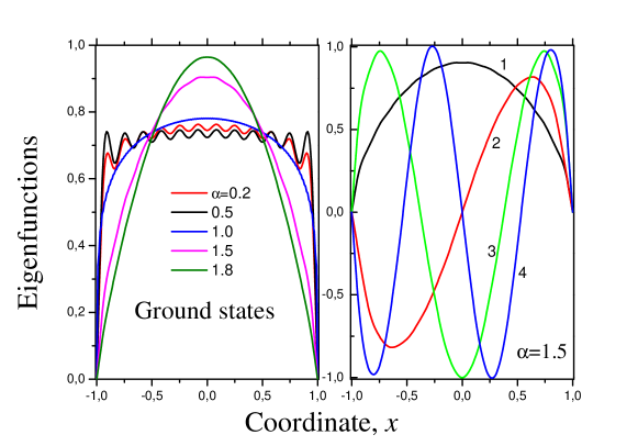
Figure 4: Left panel. Comparison of ground states for the regional fractional operator (31) for different Lévy indices $\alpha$, shown in the panel. Right panel portrays the same as in Fig. 2 but for $\alpha=1.5$. Figures near curves correspond to the number of a state.

To give a glimpse of the $\alpha$-dependence of the discussed spectral problems, in Fig. 4 we display comparatively the $n=1$ eigenfunctions (ground states) for a couple of $\alpha\neq 1$ values (the left panel). We note that for $\alpha=0.2$ and $0.5$ the ground state eigenfunctions show up an oscillatory behavior, close to a maximum. The computation has been completed for 50$\times$50 matrices (and checked for 30$\times$30, which still can be viewed to provide too rough approximation. These oscillatory artifacts are expected to smoothen down with the matrix size growth. For $\alpha=1.5$ and 1.8, curves have been evaluated by employing 50$\times$50 sized matrices, and are smooth.

The right panel of Fig. 4 depicts four lowest eigenfunctions for $\alpha=1.5$. The pertinent curves are qualitatively similar to those for $\alpha=1$, c.f. Fig. 3.

IV.3 Regional fractional Laplacian. Trigonometric base with Neumann boundary conditions - an obstacle.

On the basis of reults reported in Figs. (2) to (4), it is possible to investigate the behavior of the derivative of the ground state in the vicinity of boundary points. Clearly, $\psi_{1}^{\prime}(x\rightarrow\pm 1)$ becomes smaller as $\alpha$ increases. While for $0.2<\alpha<1$ the decay of $\psi_{1}(x)$ is steep, at $\alpha>1$ the decay becomes progressively milder. Accordingly, as $\alpha$ increases, the derivative $\psi_{n}^{\prime}(x\rightarrow\pm 1)$ of any state decreases. It is different from zero in the whole range $0<\alpha<2$.

It is thus natural to address the question of whether the traditional Neumann condition (vanishing od the derivative of the function at the boundaries) is at all feasible for the regional fractional Laplacian. The natural choice at this point is to pass from the Dirichlet to the Neumann $L^{2}([-1,1])$ basis (originally devised for the standard Laplacian in the interval, compare e.g. subsection III.B, Eqs. (24) and (25)).

The pertinent Neumann base in the interval of length $L$ comprises $f_{n}=\cos(n\pi x/L)$, $0<x<L$, $n=0,1,2,...$. In the dimensionless units (measuring $x$ in the units of $L$) the functions assume the form $f_{n}=\cos n\pi x,\ x\in[0,1],\ n=0,1,2,3,...$ This basis system is orthogonal but not normalized: $\int_{0}^{1}\cos n\pi x\cos k\pi xdx=\frac{1}{2}\delta_{nk},\ n,k\neq 0$ or $1,\quad n=k=0$. The passage to the interval [-1,1] is accomplished via a substitution $x\to(x+1)/2$, which gives rise to $f_{n}=\cos\frac{n\pi}{2}(x+1),\ n=0,1,2,...,\ x\in[-1,1]$. This basis system is orthonormal in $L^{2}([-1,1])$ except for $f_{0}=1$. After incorporating the normalization coefficient, the orthonormal base with Neumann boundary conditions at endpoints of $[-1,1])$ reads: $\{f_{0}=1/\sqrt{2},\,f_{n}=\cos\frac{n\pi}{2}(x+1),\ n=1,2,...,x\in[-1,1]\}$.

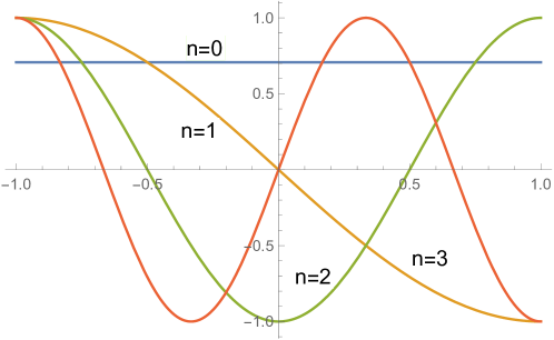
Figure 5: Plot of four first functions of the Neumann base in the interval $[-1,1]$.

The Neumann basis functions take non-zero values at the boundaries $x=\pm 1$, see e.g. Fig. 5, and this fact actually precludes the convergence of integrals that define matrix elements involved in the solution of the eigenvalue problem for the regional operator.

To demonstrate the divergence obstacle, we calculate explicitly the auxiliary function $g_{k\alpha}$ (see Eq. (15) of Ref. mypre ) for $\alpha=1$. We have

$${\color[rgb]{1,0,0}{g_{k1}}} = -\frac{1}{\pi}\int_{-1}^{1}\frac{\cos\frac{k\pi}{2}(x+1)}{(z-x)^{2}}dz=\frac{1}{\pi}\left(\frac{\cos k\pi}{1-x}+\frac{1}{1+x}\right)+\frac{k}{2}\Bigg{\{}\left[{\mathrm{Ci}}\frac{k\pi}{2}|x-1|-{\mathrm{Ci}}\frac{k\pi}{2}|x+1|\right]\sin\frac{k\pi}{2}(x+1)+$$ (46)

$$+\left[{\mathrm{Si}}\frac{k\pi}{2}(x+1)-{\mathrm{Si}}\frac{k\pi}{2}(x-1)\right]\cos\frac{k\pi}{2}(x+1)\Bigg{\}}.$$

Now, if we pass to an explicit form of the matrix elements (c.f. Eq. 18) of Ref. mypre )

$$\gamma_{kl1}=\int_{-1}^{1}\cos\frac{l\pi}{2}(x+1)g_{k1}(x)dx,$$ (47)

we see that the terms in Ex. (46), which contain $(1\pm x)^{-1}$, generate the logarithmic divergence.

The choice of $\alpha=1$ may be considered special, but explicit computations allow to identify jeopardies to be met, if the Neumann base in use. Actually, the situation is more intricate. In below we shall see that for $\alpha\geq 1$ the divergence problem persists, while for $\alpha<1$ one can handle the integrals.

Interestingly, these observations appear to stay in conformity with the mathematically rigorous discussion of divergence jeopardies in case of censored Lévy flights, bogdan , and of reflected Lévy flights proper, warma , where the stability parameter ranges $0<\alpha<1$ and $1\leq\alpha<2$ were found to refer to qualitatively different jump-type processes.

We now return to the above functions $f_{n}=\cos\frac{k\pi}{2}(x+1)$ ($k=0,1,2,...$) comprising complete orthonormal basis system in $L^{2}(D),D=[-1,1]$. While seeking a solution $\psi_{\alpha}(x)$ of the eigenvalue problem for the fractional Laplacian, we consider the expansion $\psi_{\alpha}(x)=\sum_{k=0}^{\infty}a_{k\alpha}\,f_{k}(x)$.

To quantify a possible outcome of the choice of Neumann boundary conditions, it is sufficient to consider the first integral term in Eq. (31), which is a remnant of the action of the restricted fractional Laplacian proper upon $\psi(x)$. Clearly, the second term (the inverted potential) does not depend on the choice of the (Dirichlet vs Neumann) boundary conditions.

Following the arguments of mypre , we invoke Eq. (15) therein, and note that for an auxiliary function $g_{k\alpha}(x)$ ($0<\alpha<2$) we actually have:

$$g_{k\alpha}(x)=-A_{\alpha}\int_{-1}^{1}\frac{f_{k}(u)}{|u-x|^{1+\alpha}}=\{x-u=t,\ u=x-t,\ du=dt\}=-A_{\alpha}\int_{x-1}^{x+1}\frac{f_{k}(x-t)dt}{t^{1+\alpha}}=$$

$$=-A_{\alpha}\left\{\begin{array}[]{cc}\frac{dt}{t^{1+\alpha}}=dv&u=f_{k}(x-t)\\ v=-\frac{1}{\alpha t^{\alpha}}&du=-f^{\prime}_{k}(x-t)dt\end{array}\right\}=-A_{\alpha}\left[-\frac{f_{k}(x-t)}{\alpha t^{\alpha}}\Biggl{|}_{x-1}^{x+1}-\frac{1}{\alpha}\int_{x-1}^{x+1}\frac{f^{\prime}_{k}(x-t)dt}{t^{\alpha}}\right]=$$ (50)

$$=\frac{A_{\alpha}}{\alpha}\left[\frac{f_{k}(1)}{(x-1)^{\alpha}}-\frac{f_{k}(-1)}{(x+1)^{\alpha}}+\int_{x-1}^{x+1}\frac{f^{\prime}_{k}(x-t)dt}{t^{\alpha}}\right].$$ (51)

Would we have imposed the Dirichlet boundary conditions $f_{k}(\pm 1)=0$, the first two terms in Eq. (51) would vanish, leaving us with convergent integral. In the non-Dirichlet regime the situation becomes more complicated, since we may encounter divergent matrix elements. The latter obstacle we shall analyze in more detail.

To this end let us calculate the matrix elements $\gamma_{\alpha kl}=\int_{-1}^{1}g_{k\alpha}(x)f_{l}(x)dx$ of the (so far) ordinary fractional Laplacian:

$$\gamma_{\alpha kl}=\frac{A_{\alpha}}{\alpha}\int_{-1}^{1}f_{l}(x)\left\{\frac{f_{k}(1)}{(x-1)^{\alpha}}-\frac{f_{k}(-1)}{(x+1)^{\alpha}}+\int_{x-1}^{x+1}\frac{f^{\prime}_{k}(x-t)dt}{t^{\alpha}}\right\}dx.$$ (52)

It can be shown that the double integral in Ex. (52) is convergent (of course in the sense of Cauchy principal value) for all $0<\alpha<2$. At the same time if $f_{k}(\pm 1)\neq 0$, we should consider the first two integrals separately. We have

$$I_{1}=\int_{-1}^{1}\frac{f_{l}(x)dx}{(x-1)^{\alpha}},\ I_{-1}=\int_{-1}^{1}\frac{f_{l}(x)dx}{(x+1)^{\alpha}}.$$ (53)

The ”dangerous” points are $x=1$ for $I_{1}$ and $x=-1$ for $I_{-1}$. Clearly, in the Dirichlet case $q_{l}(\pm 1)=0$, no convergence problem arises.

However, if $f_{l}(\pm 1)=const\equiv C$ (with respect to the convergence issue, it does not matter whether these constants can or cannot be different at $x=1$ and $x=-1$), we have

$$I_{1}(x\to 1)=C\int_{-1}^{1}\frac{dx}{(x-1)^{\alpha}}=C\frac{(x-1)^{1-\alpha}}{1-\alpha}\Bigg{|}_{-1}^{1}=\{x-1=\delta,\ x\to 1,\ \delta\to 0\}\sim\frac{C}{1-\alpha}\lim_{\delta\to 0}\delta^{1-\alpha}=$$

$$=\left\{\begin{array}[]{c}0,\qquad\quad\alpha<1\\ \ln\delta\to\infty,\ \alpha=1\\ \infty,\ 1<\alpha<2.\end{array}\right.$$ (57)

The same behavior is shared by $I_{-1}$ near $x=-1$. This shows that regardless the value of derivative $f^{\prime}_{l}(\pm 1)$, the integrals (53) are divergent in the range $1\leq\alpha<2$.

W point out that a departure point for our discussion was the Neumann basis system and thus standard Neumann boundary data (vanishing of the derivative at the endpoints of $[-1,1]$) were implicit. The outcome (51) tells us that the regional fractional Laplacian may react consistently to Neumann boundary data in the range $0<\alpha<1$.

This observation stays in conformity with results of mathematical papers guan ; warma , where the range $0<\alpha<1$ has been singled out for the unquestionable identification of the regional fractional Laplacian on a closed bounded domain as the generator of a reflected $\alpha$-stable process. Interestingly, no traditional form of the Neumann condition has been in use. On the other hand, a traditional looking (merely on the formal, notational level) Neumann-type boundary condition has been found to be necessary for the existence of the reflected process in the range $1\leq\alpha<1$.

V Regional fractional Laplacian: Signatures of reflecting boundaries.

The explicit spectral solution for the regional fractional Laplacian in the non-Dirichlet regime is not known in the literature, except for some general existence statements, bogdan ; guan ; warma ; grubb . The low part of that spectrum (shapes of ground and first excited eigenstates, related egenvalues) remains unkonwn as well. The spectral solution reported in duo refers explicitly to the Dirichlet boudary data for the regional fractional Laplacian.

Our major purpose is to deduce the spectral solution that would have something in common with physicists’ intuitions about reflected random motions in a bounded domain. To this end we shall address the spectral problem for the regional fractional Laplacian more carefully, avoiding the decomposition of the (nonlocal operator action-defining) integral expression into a sum of integrals, of the form (27) or (31) -(34). We shall not impose any explicit form of the Neumann condition (or any of its analogs, that can be met in the literature, guan ; warma ; barles ; dipierro ; abtangelo1 ). The only Neumann input will be related to the choice of the basis system in $L^{2}(D)$, the latter Hilbert space being not the one favoured by mathematicians guide . Lowest eigenvalues and shapes of related eigenfunctions will be deduced with a numerical assistance.

The structure of expression for fractional regional operator (31) shows that the term $\psi(x)$ balances $\psi(u)$ in the integrand numerator making the integral convergent. Indeed, by inserting $u=x+\delta$ in the integrand (31) and expanding at small $\delta=u-x$ in power series, we obtain that around the dangerous point $u=x$, the integral takes the form $\int\frac{u-x}{|u-x|^{1+\alpha}}du$, which is convergent for $0<\alpha<1$. Note that it has the form $\int dt/t^{\alpha}\sim t^{1-\alpha}=0$ at $\alpha<1$) and exists as the Cauchy principal value for $1\leq\alpha\leq 2$. We have previously discussed this question in Ref.pre11 , see Eqs. (9), (10) and surrounding discussion therein. We shall analyze that issue in more detail, in below.

Accordingly, to calculate safely (i.e. without divergencies) the spectrum of the regional operator (31), we should not split the integral into a sum of terms containing respectively $\psi(u)$ and $\psi(x)$, but rather consider them together. (We point out that in case of the restricted fractional Laplacian with Dirichlet boundary data, we were actually urged to split the integral into a sum, because the term with $\psi(x)$ has been vanishing identically in this case, see Ref. mypre for details.)

Let us make use of the modulus property

$$|u-x|=\left\{\begin{array}[]{c}u-x,\ u>x\\ x-u,\ u<x.\end{array}\right\}$$ (58)

and rewrite the limits of integration in Eq. (31) accordingly, so arriving at (once more here $D=[-1,1]$)

$$(-\Delta)^{\alpha/2}_{D,reg}\psi(x)=-A_{\alpha}\int_{-1}^{1}\frac{\psi(u)-\psi(x)}{|u-x|^{1+\alpha}}du=-A_{\alpha}\left[\int_{-1}^{x}\frac{\psi(u)-\psi(x)}{(x-u)^{1+\alpha}}du+\int_{x}^{1}\frac{\psi(u)-\psi(x)}{(u-x)^{1+\alpha}}du\right].$$ (59)

We perform the substitution $x-u=t$ ($u=x-t$) in the first integral to obtain

$$P_{1}(x)=\int_{0}^{x+1}\frac{\psi(x-t)-\psi(x)}{t^{1+\alpha}}dt.$$ (60)

Next we substitute $u-x=t$ ($u=x+t$) in the second integral:

$$P_{2}(x)=\int_{0}^{1-x}\frac{\psi(x+t)-\psi(x)}{t^{1+\alpha}}dt.$$ (61)

The regional operator can be rewritten in the form

$$(-\Delta)^{\alpha/2}_{D,reg}\psi(x)=-A_{\alpha}\bigg{[}P_{1}(x)+P_{2}(x)\bigg{]}.$$ (62)

We shall demonstrate that for $0<\alpha<1$ the integrals $P_{i}(x)$ ($i=1,2$) are convergent as $t\to 0$. We have in the lowest order in $t$

$$\psi(x-t)\approx\psi(x)-t\psi^{\prime}(x),\ \psi(x+t)\approx\psi(x)+t\psi^{\prime}(x).$$ (63)

Substitution of (63) into (60) and (61) yields

$$P_{1}(x)=-\psi^{\prime}(x)\int_{0}^{x+1}\frac{tdt}{t^{1+\alpha}}=-\psi^{\prime}(x)\left.\frac{t^{1-\alpha}}{1-\alpha}\right|_{0}^{x+1}=-\psi^{\prime}(x)\frac{(x+1)^{1-\alpha}}{1-\alpha},\ \alpha<1.$$ (64)

$$P_{2}(x)=\psi^{\prime}(x)\int_{0}^{1-x}\frac{tdt}{t^{1+\alpha}}=\psi^{\prime}(x)\left.\frac{t^{1-\alpha}}{1-\alpha}\right|_{0}^{1-x}=\psi^{\prime}(x)\frac{(1-x)^{1-\alpha}}{1-\alpha},\ \alpha<1.$$ (65)

We note that at $1\leq\alpha\leq 2$ we should interpret $P_{1}+P_{2}$ as a whole, but in terms of the Cauchy principal value procedure. The limiting behavior near zero, gives rise to the cancellation similar to that in Eq. (10) from Ref. pre11 .

In the lowest order in $t$, the final form of of the regional fractional operator reads

$$(-\Delta)^{\alpha/2}_{D,reg}\psi(x)\approx-A_{\alpha}\frac{\psi^{\prime}(x)}{1-\alpha}\biggl{[}(1-x)^{1-\alpha}-(1+x)^{1-\alpha}\biggr{]}.$$ (66)

The expression (66) is already free from divergencies.

We note that the procedure (63) can be extended to an arbitrary order in $t$ to yield the representation of the regional fractional Laplacian (nonlocal, integral operator) through the infinite series of locally defined differential operators. For our present purposes we find that ”series idea” is impractical, being too much computing time consuming. Therefore, we shall compute explicitly the integrals (59) substituting $\psi(x)$ by $f_{k}(x)$, which are the elements of the Neumann basis in $L^{2}(D)$, $n=0,1,2,...$ . We mind the structure of the integrands in Eqs (59) - (66). Namely, the Lévy index $\alpha$ is contained only in the denominators, while functions $\psi(x)$ do not have this index. The same situation occurs for the functions $f_{k}(x)$. Below, for convenience, we include index $\alpha$ in the definition of $f_{k}(x)$, i.e. we put formally $f_{k}(x)\equiv f_{k\alpha}(x)$. We have:

$$f_{k\alpha}(x)=-A_{\alpha}\bigg{[}P_{1,k\alpha}(x)+P_{2,k\alpha}(x)\bigg{]},\,\,P_{1,k\alpha}(x)=\int_{0}^{x+1}\frac{\cos\frac{k\pi}{2}(x-t+1)-\cos\frac{k\pi}{2}(x+1)}{t^{1+\alpha}}dt=$$

$$=\cos\frac{k\pi}{2}(x+1)P_{11,k\alpha}(x)+\sin\frac{k\pi}{2}(x+1)P_{12,k\alpha}(x).$$ (67)

$$P_{2,k\alpha}(x)=\int_{0}^{1-x}\frac{\cos\frac{k\pi}{2}(x+t+1)-\cos\frac{k\pi}{2}(x+1)}{t^{1+\alpha}}dt=$$

$$=\cos\frac{k\pi}{2}(x+1)P_{21,k\alpha}(x)-\sin\frac{k\pi}{2}(x+1)P_{22,k\alpha}(x).$$ (68)

$$P_{11,k\alpha}(x)=\int_{0}^{x+1}\frac{\cos\frac{k\pi t}{2}-1}{t^{1+\alpha}}dt,\ P_{12,k\alpha}(x)=\int_{0}^{x+1}\frac{\sin\frac{k\pi t}{2}}{t^{1+\alpha}}dt,$$ (69)

$$P_{21,k\alpha}(x)=\int_{0}^{1-x}\frac{\cos\frac{k\pi t}{2}-1}{t^{1+\alpha}}dt,\ P_{22,k\alpha}(x)=\int_{0}^{1-x}\frac{\sin\frac{k\pi t}{2}}{t^{1+\alpha}}dt.$$ (70)

To derive the expressions for $P_{ij,k\alpha}$ ($i,j=1,2$), we use following trigonometric identity: $\cos(A-B)=\cos A\cos B+\sin A\sin B$ so that for example in (67)

$$\cos\frac{k\pi}{2}(x+1-t)-\cos\frac{k\pi}{2}(x+1)=\cos\frac{k\pi}{2}(x+1)\cos\frac{k\pi t}{2}+\sin\frac{k\pi}{2}(x+1)\sin\frac{k\pi t}{2}-\cos\frac{k\pi}{2}(x+1)=$$

$$=\cos\frac{k\pi}{2}(x+1)\left(\cos\frac{k\pi t}{2}-1\right)+\sin\frac{k\pi}{2}(x+1)\sin\frac{k\pi t}{2}.$$

The last expression, being divided by $t^{1+\alpha}$ and integrated, yields Eq. (69) for $P_{11,k\alpha}(x)$ and $P_{12,k\alpha}(x)$. The derivation of Eqs (70) is the same. In other words, the second subscript in the functions $P_{ij,k\alpha}$ ($i,j=1,2$) appears simply because the initial functions $P_{i,k\alpha}(x)$ ($i=1,2$) (67), (68) contain two terms, each of which adds one more index $j=1,2$.

The integrals $P_{ij,k\alpha}$ ($i,j=1,2$) will be calculated numerically. For reference purposes we list the integrals $P_{ij,k\alpha}$ ($i,j=1,2$) in terms of variable $z=k\pi t/2$, which we use for actual numerical calculations

$$P_{11,k\alpha}(x)=\left(\frac{k\pi}{2}\right)^{\alpha}\int_{0}^{\frac{k\pi}{2}(x+1)}\frac{\cos z-1}{z^{1+\alpha}}dz,\ P_{12,k\alpha}(x)=\left(\frac{k\pi}{2}\right)^{\alpha}\int_{0}^{\frac{k\pi}{2}(x+1)}\frac{\sin z}{z^{1+\alpha}}dz,$$

$$P_{21,k\alpha}(x)=\left(\frac{k\pi}{2}\right)^{\alpha}\int_{0}^{\frac{k\pi}{2}(1-x)}\frac{\cos z-1}{z^{1+\alpha}}dz,\ P_{22,k\alpha}(x)=\left(\frac{k\pi}{2}\right)^{\alpha}\int_{0}^{\frac{k\pi}{2}(1-x)}\frac{\sin z}{z^{1+\alpha}}dz.$$ (71)

Also, to remove the (spurious) divergencies at $z=0$ ”gracefully”, we render the integrals to the form

$$P_{ij,k\alpha}(x)=\int_{0}^{\delta}+\int_{\delta}^{1\pm x}\equiv P_{ij,k0\alpha}(x)+\Delta P_{ij,k\alpha},\ \delta<0.01.$$ (72)

The explicit expressions for $\Delta P_{ij,k\alpha}$ read

$$\Delta P_{11,k\alpha}=\Delta P_{21,k\alpha}=\left(\frac{k\pi}{2}\right)^{\alpha}\frac{1}{2}\frac{\delta^{2-\alpha}}{2-\alpha},\ \Delta P_{12,k\alpha}=\Delta P_{22,k\alpha}=\left(\frac{k\pi}{2}\right)^{\alpha}\frac{\delta^{1-\alpha}}{1-\alpha}.$$ (73)

Finally, the elements of the matrix $(\gamma_{kl\alpha})$, to be diagonalized in order to find the desired spectrum, are as follows

$$\gamma_{kl\alpha}=-A_{\alpha}\int_{-1}^{1}\cos\frac{l\pi}{2}(x-t+1)\Bigg{\{}\cos\frac{k\pi}{2}(x-t+1)\bigg{[}P_{11,k\alpha}(x)+P_{21,k\alpha}(x)\bigg{]}+$$

$$+\sin\frac{k\pi}{2}(x-t+1)\bigg{[}P_{12,k\alpha}(x)-P_{22,k\alpha}(x)\bigg{]}\Bigg{\}}dx.$$ (74)

The results of numerical calculations of the spectrum for $(\gamma_{kl\alpha})$, (74), are reported in the Table 2. As computational times are very long (around six hours for 20x20 matrix and around 24 hours for 30x30 one), we limit ourselves for 20x20 matrices. However, the qualitative features of the spectrum remain the same as those for larger matrices. We have checked that by test calculations of some of the eigenfunctions, by means of 30x30 matrices.

$i$	1	2	3	4	5	6
$\alpha=0.2$	0.0000	0.1871	0.3075	0.3972	0.4696	0.5307
$\alpha=0.2$ duo	0.0003	0.1878	0.3085	0.3981	0.4700	0.5306
$\alpha=0.5$	0.001	0.4499	0.8505	1.1959	1.5018	1.7785
$\alpha=0.5$ duo	0.0038	0.4593	0.8626	1.2091	1.5149	1.7911
$\alpha=0.7$	0.004	0.6319	1.3138	1.9591	2.5665	3.1420
$\alpha=0.7$ duo	0.0170	0.6729	1.3646	2.0140	2.6231	3.1993
$\alpha=0.9$	0.006	0.8290	1.8987	3.0064	4.1148	5.2156
$\alpha=0.9$ duo	0.0640	0.9799	2.0823	3.2054	4.3230	5.4300

Table 2: The comparison of 6 lowest eigenvalues $E_{i}$ of the regional fractional Laplacian, evaluated in the Neumann base, for different $\alpha$ in the range $0<\alpha<1$ (calculated by means of the 20x20 matrices), with those obtained by imposing the Dirichlet boundary condition. Data are taken form Table I in Section IV of the present paper and from Table I in Ref. duo (for the comparison purpose we have abstained from using the label zero; the displayed data should be read as first, second, third… eigenvalue of the regional Laplacian in question). The first left column, modulo the computing inaccuracy, is a clear signature of reflecting boundary data that were imported by executing the the diagonalization in the Neumann basis. The ground state function in the Neumann base is constant and the respective eigenvalue should equal zero. Our data show that numerically computed lowest eigenvalue should actually be identified with zero, up to inaccuracies appearing in the third decimal place.

It seen that the Neumann base, in view of our matrix size limitations (small matrices, to lower the computing time) gives slightly inaccurate estimation for the lowest (ground state) eigenvalue . This is probably due to the fact that the lowest function of the Neumann base $f_{0}=1/\sqrt{2}$ is simply constant.

To convince ourselves that the obtained eigenvalues are signatures of reflecting boundaries, we have computed a couple of (approximate) eigenfunctions. The representative plot of four lowest eigenfunctions for $\alpha=0.5$ is portrayed in Fig. 6.

We have checked that for other $\alpha\in(0,1)$ the eigenfunctions become fairly close to those found for $\alpha=0.5$. Also, they are not distant from the Neumann basis (trigonometric) functions. Strictly speaking, up to a sign of resulting eigenfunctions $\psi_{n}$ may happen to be opposite to that of the Neumann trigonometric ones. Except for the ground state, the sign issue is immaterial, sine it is $|\psi_{n}|^{2}$ which stands for the probability density.

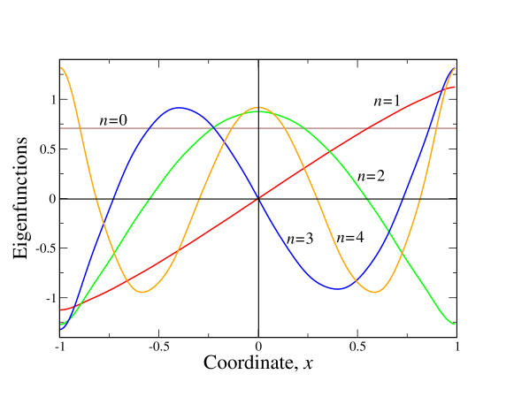
Figure 6: The representative ($\alpha=0.5$) plot of the first five eigenfunctions of the regional fractional Laplacian, found via the diagonalization in the Neumann base; $n=0$ function is constant, being a clear signature of the reflecting boundary conditions. The corresponding eigenvalue is fapp (for all practical purposes) zero. It is instructive to compare the shapes of eigenfunctions with the elements of the Neumann base, depicted in Fig. 5.

The main feature of the eigenfunctions is that appear to satisfy the Neumann boundary conditions, intepreted in terms of standard vanishing derivatives.

We have paid special attention to the range $0<\alpha<1$, because in this parameter regime the integrals (53) are convergent. The case of $1<\alpha<2$ needs more attention, since these integrals exist only in the sense of Cauchy principal value. That enforces slight modifcations of the matrix diagonalization procedure, previously adopted to calculate the spectrum of the regional fractional Laplacian in the Neumann base .

On one hand, the calculation of the matrix elements (integrals) is now more time consuming, beacuse we need to bypass the singularity at $u=x$ by means of the Cauchy principal value. On the other hand, the convergence of the matrix method is generally much worse for the base with Neumann boundary conditions than that for Dirichlet ones.

For instance, for the Dirichlet base, the acceptable accuracy of computation outcomes has been achieved already for 20x20 matrices. For the Neumann base we need matrices of the size 1000x1000 to achieve an acceptable accuracy level (the least possible case is 600x600). That substantially increases the computational time. The integration procedure for $1<\alpha<2$ incurs further increase of the computation time.

By these reasons, we have explicitly checked the signatures of reflection by an explicit computation of the ground state eigenvalue for $\alpha=1.2$, 1.5 and 1.8, followed by a computation of the shape of the corresponding eigenfunction. As expected, the eigenvalues come up (for all practical purposes) as zero, and eigenfunctions are indeed constant.

In passing, we note, that the integrals (53) are identically zero for the constant function $\psi(x)$. This is actually the signature of reflection, i.e. the zeroth ground state eigenvalue.

VI On impenetrable barriers for Lévy flights: comments on the stochastic behavior in the vicinity of the boundary.

The notion of censored stable processes, as introduced in Ref. bogdan is verbally rather loose: a censored stable process in an open set $D\subset R^{n}$ is obtained by suppressing its jumps from D to the complement $R^{n}\backslash D$. Alternatively, it is a process ”forced” to stay inside $D$. Jumps are censored, i.e. these that would (according to the jump-size probability law) ”land” beyond $D$ are simply cancelled. Next the process is resurrected at the stopping point and started anew. In connection with the resurrection of Markov process se e.g. bogdan ; pakes .

Remark 10: The above concept of resurrection, exploits the ”starting anew” property for the stopped stochastic process. It shows some affinity with the family of stochastic processes with resetting, where the wandering particle can be reset to an initial location, at a certain rate, and next the process is started anew. It is known that in the diffusion with stochastic resetting one arrives at nonequilibrium stationary states with non-Gaussian fluctuations for the particle position. Apart form the above (reset) affinity, we have not found any ”probability accumulation” outcomes that would resemble those reported in dybiec ; dybiec1 and in the fractional Brownian motion on the interval, metzler2 .

The Authors of Ref. bogdan exclude from considerations so-called taboo processes which are related to the concept of the Doob $h$-transform, gar1 ; mazzolo ; pinsky and are known not to leave the open set $D$. It is demonstrated that what is named in Ref. bogdan a censored processes (actually, a recurrent censored symmetric $\alpha$-stable process) is different (in law) from the conditioned not to leave $D$ symmetric stable one, c.f. pp. 104-105 in Ref. bogdan . That is by no mean a no-go statement for taboo processes, quite simply they do not involve any point-wise censoring mechanism, since it is the conditioning that does the job (of not reaching the boundaries).

It is quite clear, that the above loose definition encompasses both taboo and censored processes, plus (upon admitting that the boundary of $D$ can be reached by the process) $\alpha$-stable versions of reflected processes. The main issue addressed in the mathematical literature has been to strengthen the concept of ”reflection” by inventing nonlocal analogs of Neumann boundary conditions, guan ; barles ; warma ; dipierro ; abtangelo1 .

Various scenarios of the behavior of the censored process in the vicinity of the boundary have been formulated as well. One of them has been verbalized as follows, dipierro ; abtangelo1 : when the process exits $D$, it immediately comes back to $D$. The way it comes back is: if a process exits to a point $x\in R^{n}\backslash\overline{D}$, its return to $y\in D$ is realized with a probability density being proportional to $|x-y|^{-n-\alpha}$, hence not necessarily to the stopping point.

A concept of the resurrection for a Markov process has been invoked here as well, bogdan ; pakes . It amounts to an immediate resurrection of the process after eliminating (censorship) the inadmissible jump (form $D$ to $R^{n}\backslash D$), through a procedure of gluing together stable processes: at a stopping point (and time) of the tentativelyy terminated process, we glue its copy that actually gives birth to a process started anew at the stopping point. The process proceeds proceed up to the next stopping time (i.e censored jump), and the gluing procedure is repeated. Such continually resurrected process is bound not to leave $D$, as required.

Leaving aside a great amount of technicalities concerning the proper mathematical formulation of what a reflected stable process should actually be, we shall pass to a brief discussion of physicists’ viewpoint on impenetrable barriers and eventually on the concept of reflection (e.g. that of reflecting boundaries), gitterman ; buldyrev , dybiec -denisov .

Motivated by the path-wise simulations, physicists coin their own recipies on how to implement the condition of reflection from the barrier in terms of the the sample path behavior (that on the computer simulation level). For example, in Ref. dybiec the condition of reflection is assured by wrapping the trajectory, destined to hit the barrier (or crossing the barrier), around the hitting point location, while preseving the assigned length. On the other hand, it is mentioned that for jump-type processes the location boundary is not hit by the majority of discontinuous sample paths and returns (or recrossings the boundary location) should be excluded from considerations, which excludes the wrapping scenario form further considerations.

Another viewpoint mentioned in Ref. dybiec refers to a simulation of the reflecting boundary by an infinitely high hard (e.g. impenetrable) wall, quantum mechanically interpreted as the infite well (zaba0 ; zaba1 ), yielding an immediate reflection once its vicinity (and not necessarily the boundary itself) is reached.

On the other hand, in Ref. dybiec1 another proposal for the introduction of the reflection scenario has been outlined (an idea inspired by broeck ; denisov ; dubkov ), with a focus on a numerical simulation of sample trajectories of the Langevin-type Lévy - stable evolution in the binding extremally anharmonic potential $V_{n}(x)\sim x^{n}$ with $n\gg 1$ (set e.g. $n=800$ for concretness).

Here a departure point is an observation (strictly speaking, questionable in the quantum setting) that in the limit $n\rightarrow\infty$ the potential $V_{n}(x)$ mimics the infnite well enclosure, with boundaries at endpoints of the interval $[-1,1]$ (interpreted in dybiec1 as reflecting). The random motion is described in terms of the Langevin-type equation $dX(t)/dt=-{V^{\prime}}_{n}(x)+\zeta_{\alpha}(t)$ where $\zeta_{\alpha}(t)$ is a formal encoding of the symmetric white $\alpha$-stable noise, c.f. dybiec1 . The limiting stationary probability density of the associated fractional Fokker-Planck equation has been found denisov in the form of the $L^{1}([-1,1]$ normalized function :

$$\rho_{\alpha}(x)=(2)^{1-\alpha}{\frac{\Gamma(\alpha)}{\Gamma^{2}(\alpha/2)}}(1-x^{2})^{\alpha/2-1},$$ (75)

the result valid for all $0<\alpha\leq 2$. The special case of the Cauchy noise ($\alpha=1$) has been addressed in Ref. dubkov , by an independent reasoning, with the outcome:

$$\rho_{1}(x)={\frac{1}{\pi}}{\frac{1}{\sqrt{1-x^{2}}}}$$ (76)

valid for all $|x|<1$. This function blows up to infinity at the boundaries of the interval $[-1,1]$.

In passing we note that for $\alpha=2$ a uniform Brownian distribution $1/L$ arises. That would suggest a link with reflected processes, but this observation is misleading.

The probability density functions (75), (76), do not belong to the $L^{2}([-1,1])$ inventory associated with the regional fractional Laplacian. More than that, they refer to ranom motion scenarios that cannot reach the boundary and definitely comply with the stopping scenarios used in the numerical simulations in Ref. dybiec1 . That view is supported by the fact that (76) coincides with the familiar probability distribution function for the classical harmonic oscillator. Its high probability areas correspond to the long residence time for a classical particle in harmonic motion.

From the physical point of view, the most interesting observation of Ref. dybiec1 in this context is that the extremely anharmonic and stopping motion scenarios in the presence of the symmetric $\alpha$-stable noise, actually yield the same statistics of simulation outcomes, c.f., Section II.A.2 in dybiec1 . Moreover, a detectable deviation from these outcomes has been reported if the wrapping scenario is employed. Actually, irrespective of the stability index $\alpha$, the wrapping assumption, in the path-wise simulation procedure of Refs. dybiec ; dybiec1 has been found to lead to a uniform asymptotic distribution in the interval, like in the reflecting Brownian motion. The pertinent figures have not been reporoduced in Ref. dybiec1 , but are available from the Authors, dybiec2 .

At this point we shall verbalize the concept of the stopping scenario, dybiec2 . In the course of the path-wise simulation of the jump-type process, any jump longer than the distance of the point of origin from the boundary is cancelled (the process is stopped). In the $\varepsilon$-vicinity of the boundary, $\epsilon\ll 1$ all jumps in the direction of the barrier are cancelled (it is an explcit censorship at work). The process is kept stopped until the probability law will produce a jump in the direction opposite to the boundary, and next continued.

From a mathematical point of view it is clear that probability functions (75), (76) are not eigenfunctions of the regional fractional Laplacian. Actually, after completing them in $R\backslash(-1,1)$ by assigning them the value zero beyond $(-1,1)$, we realize that $\rho_{\alpha}(x)$ is the so-called $\alpha$-harmonic eigenfunction of the original fractional Laplacian $(-\Delta)^{\alpha/2}$, Eq. (1), defined on the whole of $R^{1}$ and associated with the eigenvalue zero:

$$(-\Delta)^{\alpha/2}\rho_{\alpha}(x)=0$$ (77)

c.f. what ; kulczycki . One should keep in mind that the above idenity needs somewhat involved calculations in case of arbitrary $1<\alpha<2$, but can be straightforwardly checked in case of $\alpha=1$. The calculation exploits in full a nonlocality of the fractional Laplacian, and terms that account for $R\{(-1,1)$ cannot be disregarded, dyda ; private .

Thus a stochastic process that is consistent with the pdf (76) is not the reflected one, but rather the censored one, see e.g. also bogdan . The pertinent censored process never crosses or reaches the boundary, which is a property shared with taboo processes in the impenetrable enclosure, c.f. the fractional infnite square well spectral problem or the related taboo process in the interval (so-called ground state process), zaba0 ; zaba1 ; mypre0 ; mypre ; duo ; duo1 ; gar . Nonetheless, the associated stationary probability distributions appear to be very diferrent, behaving reciprocally at the boundary: quick decay with a lowering distance from the boundary $\sim(dist)^{\alpha/2}$ (taboo process), versus blow up to infinity $\sim 1/(dist)^{\alpha/2-1}$ in the same regime (censored process). Clearly, the taboo case refers to a probability depletion in the vicinity of the boundary, while its accumulation close to the boundary characterizes the considered censored process.

VII Outlook and prospects: Some advantages of the spectral lore for fractional Laplacians in bounded domains.

VII.1 General considerations

We have paid special attention to spectral problems involved with nonlocal motion generators (fractional Laplacians of arbitrary Lévy index $0<\alpha<2$), whose adjustment to account for finite (bounded) spatial geometries is a source of ambiguities in the physical literature. Like in case of standard diffusion processes, lowest eigenfunctions and eigenvalues of the pertinent operators, are decisive for deducing measurable properties of relaxation processes towards equailibrium or their near-equilibrium behavior.

Our motivations stem basically from a simply looking inquiry into the problem of all admissible stochastic processes in a bounded domain, that may be consistently associated (derived or inferred from) with the primordial Lévy noise. That sets the broad conceptual context of Lévy flights in bounded domains and directly involves a delicvate issue of properly defined boundary data for fractional Laplacians in finite geometries.

To this end, we have adopted the numerically assisted approach to the eigenvalue problem of fractional Laplacians in the interval, developed by us earlier mypre0 and based on the expansion of the sought-for eigenfunctions in the properly tailored orthonormal base of $L^{2}(D)$. In the present paper, we have considered two such bases, namely trigonometric ones associated with $D=[-1,1]$.

The first one is familiar from the standard quantum mechanical infinite well problem land3 and comprises functions with Dirichlet boundary conditions, i.e. vanishing at the boundaries. The second one is that obeying the Neumann boundary conditions, i.e. basic functions are allowed to take arbitrary non-zero values at the boundaries, while their derivatives are required to vanish. In both cases the spectral fractional Laplacian (see Section II) simply imports all basic properties of the standard Laplacian. Things become complicated if other definitions of the fractional Laplacian in $D$ are considered.

In the course of the study, we have demonstrated that the Dirichlet base secures much better convergence properties of the numerical procedure, than the Neumann one. The latter base implies particularly bad convergence properties in the stability parameter range $1<\alpha<2$, where integrals of importance (see, e.g., Eq. (59)) exist only in the sense of Cauchy principal values. Not incidentally, in all studies devoted to censored stochastic processes, bogdan ; guan , the range $0<\alpha\leq 1$ has been considered separately from that of $1<\alpha<2$, in which major difficulties were encountered, while attempting to give meaning to the notion of reflected jump-type processes and to devise a consistent form of Neumann boundary data.

We note in passing that in so-called fractional quantum mechanics laskin , the range $1\leq\alpha<2$ is introduced a priori as the one in which this theory is supposed to make sense (it is not quite necessary assumption stef that essentially narrows the framework). We point out that a good reason for that may be the nonexistence of probability currents out of the pertinent range stef . Notwithstanding, consistent spectral solutions for Laplacians in bounded Dirichlet domains are known to exist in the whole range $0<\alpha<2$). On the other hand, spectral problems beyond the range $0<\alpha<1$, make the Dirichlet boundary data the only (for all practical purposes) reliable choice, against the Neumann or Robin ones), by purely pragmatic reasons. That conforms with the standard quantum mechanical approach, where Neumann or Robin boundary data are definitely out of favor, while the Dirichlet data are prevalent.

To the contrary, all these data are often encountered and amply discussed in the theory of Brownain motion and diffusion-type processes. In connection with the eigenvalue problems addressed, we note that one may in principle invoke the variational approach, which is customary in the ordinary quantum mechanics. Such approach works for self-adjoint operators (see, e.g. bershub ) and hence should be valid for trial functions both with Dirichlet and Neumann boundary conditions in more general than the standard Laplacian settings, i.e. for fractional Laplacians as well. It would be interesting to study the accuracy of the variational method for our two classes of (trigonometric) trial functions.

VII.2 Fractional spectral problems: Exemplary association with realistic physical systems.

Our discussion of section III on relevance versus irrelevance of eigenvalue problems for fractional Laplacians, pertains to an interplay (intertwine) between the theory of stochastic processes (stochastic modeling) in a bounded domain and the fractionally generalized quantum model-systems (that refers to so-called fractional quantum mechanics, laskin0 ; laskin1 ; laskin , see also stef ) which are spatially confined. Leaving aside an explicit probabilistic (stochastic processes) viewpoint, the developed formalism can be applied to physical systems of confined geometry (like quantum wells and/or surfaces or interfaces), where the disorder and other kinds of intrinsic randomness (hence the fractional Léy noise) can be interpreted on the quantum level.

One class of such systems is an electronic ensemble, which tunnels through potential barriers in so-called spintronic devices (see zu ; gvi ; sar and references therein). One of the realistic examples here is heterostructures like the LaAlO₃/SrTiO₃ interface oh ; sd1 ; sd2 . To describe the experimental data related to above tunneling statistics, fractional derivatives should be introduced in the conventional quantum-mechanical problem of a tunneling particle.

To be specific, the fractional generalization of the Schrödinger equation, describing the electronic properties of a hetero-junction between materials 1 and 2, reads (see Ref. sd1 for details)

$$\mathcal{H}\Psi(z)\equiv\left(\begin{array}[]{cc}s_{c}(z)+U(z)&iv(-\Delta)^{1/2}\\ iv(-\Delta)^{1/2}&-s_{v}(z)+U(z)\end{array}\right)\left(\begin{array}[]{c}\varphi(z)\\ \chi(z)\end{array}\right)=\varepsilon\left(\begin{array}[]{c}\varphi(z)\\ \chi(z)\end{array}\right),$$ (78)

where $\varepsilon$ is eigenenergy and $\Psi(z)$ is the spinor wave function of the electron at the interface. Here, $(-\Delta)^{1/2}$ is the fractional Laplacian for Lévy index $\alpha=1$, $z$ is the dimensionless coordinate along the interface (normalized by the interface width $a$) sd1 and we use atomic units $\hbar=c=1$. The spatial confinement of the problem lie in the interfacial potential $U(z)$

$$U(z)=U_{0}\delta(z)+U_{1}P(z),$$ (79)

$$P(z)=\left[\theta(z)+\theta(d-z)\right],$$

where the first term, containing $\delta$ - function, signifies the potential barrier exactly at the interface, while the second term denotes the barrier of height $U_{1}$ and width $d$, through which the electrons can tunnel. Here $\theta(z)$ is the Heaviside (unit step) function. The influence of technologically unavoidable disorder is modeled by the introduction of fractional derivative $(-\Delta)^{1/2}$ instead of ordinary gradient $d/dz$. Our further notations are as follows sd1

$$s_{c}(z)=s_{c1}[1-\theta(z)]+s_{c2}\theta(z),$$

$$s_{v}(z)=s_{v1}[1-\theta(z)]+s_{v2}\theta(z),$$

$$v(z)=v_{1}[1-\theta(z)]+v_{2}\theta(z),$$ (80)

with

$$s_{c1,2}=\Delta_{1,2}+\frac{k_{\perp}^{2}}{2m_{c1,2}},\ s_{v1,2}=\Delta_{1,2}+\frac{k_{\perp}^{2}}{2m_{v1,2}},$$ (81)

where $\Delta_{1,2}$ and $m_{c,v,1,2}$ are, respectively, the energy gaps and effective masses of interface-forming semiconductors 1 and 2. Indices $c$ and $v$ mean, respectively, the conduction and valence bands so that $m_{1c}$ denotes the electron effective mass in the conduction band of semiconductor 1, see Refs. sd1 ; sd2 for details. Also, $k_{\perp}$ is (unimportant for the interfacial problem) the electron momentum component, parallel to the interface sd1 .

The explicit form of the Schrödinger equation (78) reads

$$(s_{c}+U-\varepsilon)\,\varphi+iv(-\Delta)^{1/2}\chi=0,$$ (82)

$$iv(-\Delta)^{1/2}\varphi+(-s_{v}+U-\varepsilon)\,\chi=0.$$

Then we can express component $\chi$ through $\varphi$ from second equation (82) to obtain following eigenproblem for $\varphi$

$$(s_{c}(z)+U(z))\,\varphi(z)+v(z)(-\Delta)^{1/2}\left[\frac{v(z)}{-s_{v}(z)+U(z)-\varepsilon}\,(-\Delta)^{1/2}\varphi(z)\right]=\varepsilon\varphi(z).$$ (83)

We note that the eigenproblem (83) is indeed nonlinear as the eigenenergy $\varepsilon$ enters also the denominator. Our analysis shows that for small $\varepsilon$ the problem (83) is reducible to that for 1D regional fractional derivative. The best way to solve it is to expand a solution in the orthogonal set of functions with Neumann boundary conditions. The complete solution of the problem (83) can be obtained only numerically. Our preliminary studies of that solution show that it describes many experimentally observable salient features of the interfaces like high electronic concentration at the interface (leading, e.g. to metallic conductivity, see oh and references therein), which appears due to disorder, described by fractional derivatives. The work in this interesting direction is underway and results will be published elsewhere.

One more interesting physical problem is the onset of a chaos in excitons, induced by Rashba spin-orbit interaction br . This situation is described by one more ”confined” (although in two dimensions, making the solution to be much more complicated than in 1D case) problem. Namely, then one is dealing with the quantum version of the Kepler problem, i.e.hydrogen atom, see, e.g. ash . The fractional Hamiltonian of the 2D problem has the form

$$\frac{(-\Delta)^{\alpha/2}}{2m}\psi(x,y)-\frac{\psi(x,y)}{r}=E\psi(x,y),$$ (84)

where $r=(x^{2}+y^{2})^{1/2}$ and we once more use atomic units. Here, the spatial confinement is due to the Coulomb potential $1/r$. Similar to the case of ordinary quantum mechanics land3 ; bershub , the discreet spectrum exists only at $E<0$. It can be shown that the problem (84) admits the separation of angular and radial variables, leaving us with ordinary differential equation for the function $\psi(r)$. The solution of latter problem is still much more complicated then those in 1D. Our preliminary analysis shows that the function $\psi(r)$ can be obtained as the expansion of the complete set of eigenfunctions, corresponding to the ”ordinary” (i.e. with conventional Laplacian in Eq. (84)) 2D hydrogen atom. The method is similar to that of Ref. mypre0 . Note that the problem (84) can be formulated in 3D with additional confinement in the potential well. Latter case corresponds to the excitons, confined to quantum wells in disordered semiconductors. One more way of problem (84) generalization is to take into account the fractional analog of Rashba spin-orbit interaction br . Although the latter problem becomes very complex (for example it contains now, similar to Eq. (78), spinor wave function), its solution can be obtained along the lines of Ref. mypre0 , i.e. by the expansion over properly tailoed orthonormal basis with Dirichlet boundary conditions. The discussed problems, related to fractionally quantized Kepler one, are extremely important for photovoltaic applications (see Ref. pho for appropriate references), where possible chaotic behavior she1 ; she2 can disrupt the solar cell functionality. Namely, the chaotic behavior has been obtained explicitly in the form of ”messy” electronic trajectories she1 . At the same time, in the quantized version only weak effects like energy levels repulsion have been revealed she2 . It is tempting to expose the quantum chaotic features (along with direct quantum trajectories simulations) of this problem by substitution of the ordinary 2D Laplacian by the fractional one in the Schrödinder equation (84). In this case, the levels repulsion and other features like non-Poissonian energy level statistics rei would heavily depend on the Lévy index $\alpha$.

Acknowledgment: We would like to thank Professors K. Bogdan and G. Grubb for correspondence on censored and reflected jump-type processes, Yanzhi Zhang for explanations concerning Ref. duo , B. Dybiec for explanations concerning the stopping scenario of Refs. dybiec ; dybiec1 , R. Metzler for reference suggestion and A. Pakes for providing access to his publication on killing and resurrection of Markov processes, pakes .

References

- (1) Z. Schuss, Brownian dynamics at boundaries and interfaces, Springer, NY, 2013.
- (2) H. S. Carlsaw and J. C. Jaeger, Conduction of heat in solids, (Oxford Univ. Press, London, 1959).
- (3) D. S. Grebenkov, ”NMR survey of reflected Brownian motion”, Rev. Mod. Phys. 79, 1077, (2007).
- (4) D. S. Grebenkov, ”Laplacian eigenfunctions in NMR. I. A numerical tool”, Concepts Magn. Reson. A 32, 277, (2008)
- (5) D. S. Grebenkov, ”Laplacian Eigenfunctions in NMR. II. Theoretical Advances”, Concepts Magn. Reson., A 34, 264, (2009).
- (6) D. S. Grebenkov and B.-T. Nguyen, ”Geometrical Structure of Laplacian Eigenfunctions”, SIAM Review, 55(4), 601, (2013).
- (7) T. Bickel, ”A note on the confined diffusion”, Physica A 377, 24, (2007).
- (8) V. Linetsky, ”On the transition densities for reflected diffusions”, Adv. App. Prob. 37, 435-460, (2005)
- (9) H. Risken, The Fokker-Planck equation, (Springer, Berlin, 1996).
- (10) K. Kaleta and J. Lőrinczi, ”Transition in the decay rates of stationary distributions of Lévy motion in an energy landscape”, Phys. Rev. E 93, 022135, (2016).
- (11) M. Gitterman, ”Mean first passage time for anomalous diffusion”, Phys. Rev. E 62, 6065, (2000).
- (12) S. V. Buldyrev et al., ”Average time spent by Lévy flights and walks on an interval with absorbing boundaries”, Phys. Rev. E 64, 041108, (2001).
- (13) P. Garbaczewski and V. Stephanovich, ”Lévy flights in inhomogeneous environments”, Physica A 389, 4419, (2010).
- (14) P. Garbaczewski, W. Stephanovich, ”Lévy targeting and the principle of detailed balance”, Phys. Rev. E84, 011142 (2011)
- (15) P. Garbaczewski, ”Fractional Laplacians and Lévy flights in bounded domains”, Acta Phys. Pol. B 49(5), 921, (2018)
- (16) P. Garbaczewski, ”Killing (absorption) versus survival in random motion”, Phys. Rev. E 96, 032104, (2017).
- (17) A. Mazzolo, ”Sweetest taboo processes”, J. Stat. Mech. (2018) 073204.
- (18) R. G. Pinsky, ”On the convergence of diffusion processes conditioned to remain in a bounded region for large time to limiting positive recurrent processes”, Annals of Probability, 13 (2), 363, (1985).
- (19) W. Bao, X, Ruan, J. Shen and C. Sheng, ”Fundamental gaps of the fractional Schrödinger operator”, arXiv:1801.06517.
- (20) K. Kaleta, ”Spectral gap lower bound for the one-dimensional fractional Schrödinger operator in the interval ”, Studia Math. 209, 267, (2012).
- (21) R. Frank, ”Eigenvalue bounds for the fractional Laplacian: A review”, in: G. Palatucci, T. Kuusi (Eds.), Recent Developments in Nonlocal Theory, pp. 210–235. De Gruyter, Berlin, 2018.
- (22) H.G. Sun et al, ”A new collection of real world applications of fractional calculus in science and engineering”, Commun. Nonlinear Sci. Numer. Simulat. 64, 213, (2018).
- (23) F. A. Oliveira et al., ”Anomalous diffusion: A basic mechanism for the evolution of inhomogeneous systems”, Front. Phys. 7:18, (2019), doi: 10.3389/fphy.2019.00018
- (24) D. del-Castillo-Negrete, ”Fractional diffusion models of nonlocal transport”, Physics of Plasmas, 13, 0822308, (2006).
- (25) N. Laskin, ”Fractional Schrödinger equation”, Phys. Rev. E 66, 056108, (2002).
- (26) N. Laskin, ”Fractional quantum mechanics and Lévy path integrals”, Phys. Lett. A 268, 298, (2000).
- (27) N. Laskin, Fractional quantum mechanics, (World Scientific, Singapore, 2018).
- (28) C. Bucur and E. Valdinoci, Nonlocal diffusion and applications, Lecture Notes of the Unione Matematica Italiana, vol. 20, (Springer International Publishing Switzerland, 2016).
- (29) J. L. Vázquez, ”The Mathematical Theories of Diffusion: Nonlinear and Fractional Diffusion”, in: M. Bonforte, G. Grillo (Eds.), Nonlocal and Nonlinear Diffusions and Interactions: New Methods and Directions, Lecture Notes in Mathematics vol. 2186, (Springer, NY, 2017)
- (30) N. Abatangelo and E. Valdinoci, ”Getting acquainted with the fractional Laplacian”, arXiv:1710.1156.
- (31) A. Lischke et al, ”What is the fractional Laplacian”, arXiv:1801.09767.
- (32) R. Servadei and E. Valdinoci, ”On the spectrum of two different fractional operators”, Proceedings of the Royal Society of Edinburgh Section A: Mathematics, 144(4), 831, (2014).
- (33) B. Dybiec, E. Gudowska-Nowak and P. Hänggi, ”Lévy-Brownian motion on finite intervals: Mean-first passage time analysis”, Phys. Rev. E 73, 046104, (2006).
- (34) B. Dybiec, E. Gudowska-Nowak, E. Barkai and A. A. Dubkov, ”Lévy flights versus Lévy walks in bounded domains”, Phys. Rev. E 95, 052102, (2017).
- (35) A. A. Kharcheva et al, ”Spectral characteristics of steady-state Lévy flights in confinement potential profiles”, J. Stat. Mech. vol. 2016 (5),054039.
- (36) V. Balakrishnan, C. Van den Broeck and P. Hänggi, ”First-passage times of non-Markovian processes: The case of reflecting boundary”, Phys. Rev. 38, (8), 4213, (1988).
- (37) S. I. Denisov, W. Horsthemke and P. Hänggi, ”Steady-state Lévy flights in a confined domain”, Phys. Rev. E 77, 061112, (2008).
- (38) K. Bogdan, K. Burdzy and Z.-Q. Chen, ”Censored stable processes”, Probab. Theory Relat. Fields, 127, 89, (2002).
- (39) Q.-Y. Guan & Z.-M. Ma, ”Reflected symmetric -stable processes and regional fractional Laplacian”, Probab. Theory Relat. Fields 134, 649 (2006).
- (40) Q.-Y. Guan & Z.-M. Ma, ”Boundary problems for fractional Laplacians”, Stochastics and Dynamics, 5(3), 385, (2005)
- (41) M. Warma, ” A fractional Dirichlet-to-Neumann operator on bounded Lipschitz domains”, Commun. Pure Appl. Analysis, 14(5), 2043, (2015).
- (42) B. Barles, E. Chasseigne, C. Georgelin and E. R. Jacobsen, ”On Neumann problems for non-local equations set in a half-space”, Trans. Amer. Math. Soc. 366, 4873, (2014).
- (43) S. Dipierro, X. Ris-Oton and E. Valdinoci, ”Nonlocal problems with Neumann boundary conditions”, Revista Matematica Iberoamericana 33(2), 377, (2017).
- (44) N. Abtangelo, ”A remark on nonlocal Neumann conditions for the fractional Laplacian”, arXiv:1712.00320, (2018).
- (45) G. Grubb, ”Fractional-order operators : Boundary problems, heat equations”, arXiv:1712.01196, to appear in Springer Proceedings in Mathematics and Statistics: ”New Perspectives in Mathematical Analysis - Plenary Lectures, ISAAC 2017, Vaxjo Sweden”.
- (46) P. Garbaczewski, M. Zaba, ”Nonlocal random motions and the trapping problem”, Acta Phys. Pol. B 46, 231 (2015).
- (47) A. H. O. Wada and T. Vojta, ”Fractional Brownian motion with a reflecting wall”. Phys. Rev. E 97, 020102, (2018).
- (48) M.-C. Néel, L. Di Pietro and N. Krepysheva, ”Enhanced diffusion in a bounded domain”, IFAC Proceedings Volumes, 39(11), 448, (2006).
- (49) A. Compte, R. Metzler and J. Camacho, ”Biased continuous time random walks between parallel plates”, Phys. Rev. E 56(2), 1445, (1996).
- (50) R. Metzler and J. Klafter, ”Boundary value problems for fractional diffusion equations”, Physica A 278, 107, (2000).
- (51) B. Beumer, M. Kovács, M. M. Meerschaert and H. Sankaranarayanan, ”Reprint of: Boundary conditions for fractional diffusion”, J. Comput. Applied Math., 339, 414, (2018).
- (52) S. A. McKinley and H. Nguyen,”Anomalous diffusion and the Generalized Langevin Equation”, SIAM J. Math. Analysis 50 (5), 5119, 2017).
- (53) M. H. Vainstein et al., ”Non-exponential relaxation for anomalous diffusion”, Europhys Lett. 73 (5), 726, (2006).
- (54) T. Guggenberger et al., ” Fractional Brownian motion in a finite interval:Correlations effect, depletion or accretion zones of particles near boundaries, New Journal of Physics, 21, 022002, (2019).
- (55) M. Kwaśnicki, ”Ten equivalent definitions of the fractional Laplace operator”, Fractional Calculus & Applied Analysis, 20(1), 7, (2017).
- (56) M. Kwaśnicki, ”Fractional Laplace operator and its properties”, in: ”Handbook of fractional calculus with applications”, vol. 1, (Eds.) A. Kochuba and Y. Luchko, de Gruyter, Berlin, 2019, to be published.
- (57) R. Song and Z. Vondracek, ”Potential theory of subordinate killed Brownian motion in a domain”, Probab. Theory. Relat. Fields, 125, 578, (2003).
- (58) T. Kulczycki, ”Eigenvalues and Eigenfunctions for Stable Processes”, chap. 4, pp. 73-86, in: K. Graczyk and A. Stos (Eds.), ”Potential Analysis of Stable Processes and its Extensions”, LNM vol. 1980, (Springer-Verlag, Berlin, 2009).
- (59) S. Duo, H. Wang and Y. Zhang, ”A comparative study of nonlocal diffusion operators related to the fractional Laplacian”, Discrete & Continuous Dynamical Systems - B 22(11), 1, (2018).
- (60) S. Duo and Y. Zhang, ”Computing the ground and first excited states of the fractional Schröodinger equation in an ininite potential well”, Commun. Comput. Phys., 18, 321-350, (2015).
- (61) M. Żaba and P. Garbaczewski, ”Solving fractional Schrödinger-type spectral problems: Cauchy oscillator and Cauchy well”, J. Math. Phys. 55, 092103, (2014).
- (62) M. Żaba and P. Garbaczewski, ”Nonlocally induced (fractional) bound states: Shape analysis in the infinite Cauchy well”, J. Math. Phys. 56, 123502, (2015).
- (63) E. V. Kirichenko, P. Garbaczewski, V. Stephanovich and M. Żaba, ”Lévy flights in an infnite potential well as a hypersingular Fredholm problem”, Phys. Rev. E 93, 052110, (2016).
- (64) E. V. Kirichenko, P. Garbaczewski, V. Stephanovich and M. Żaba, ”Ultrarelativistic (Cauchy) spectral problem in the infinite well”, Acta Phys. Pol. B 47(5), 1273-1291, (2016).
- (65) N. Cusimano, F. del Teso, L. Gerardo-Giorda and G. Pagnini, ”Discretizations of the Spectral Fractional Laplacian on General Domains with Dirichlet, Neumann, and Robin Boundary Conditions”, SIAM j. Numer. Anal., 56(3), 1243, (2018).
- (66) R. Musina and A. I. Nazarov, ”On fractional Laplacians”, Comm. Partial. Diff. Eqs. 39(9), 1780, (2014).
- (67) P. Kim, R. Song and Z. Vondracek, ”On the boundary theory of subordinate killed Lévy processes”, arXiv: 1705.02595, (2017).
- (68) Y. Luchko, ”Fractional Schrödinger equation for a particle moving in a potential well”, J. Math. Phys., 54, 012111, (2013).
- (69) S. S. Bayin, ”Consistency problem of the solution of the space fractional Schrödinger equation”, J. Math. Phys., 54, 092101, (2013).
- (70) Y. Wei, ”The infinite square well problem in standard, fractional and relativistic quantum mechanics”, Int. J. Theor. Math. Phys, 5(4), 58, (2015)
- (71) K. Kaleta, M. Kwaśnicki and J. Małecki, ”Asymptotic estimate of eigenvalues of pseudo-differential operators in an interval”, J. Math Anal. Appl., 439, 896, (2016).
- (72) T. Kulczycki, M. Kwaśnicki, J. Małecki and A. Stos, ”Spectral properties of the Cauchy process on half‐line and interval”, Proc. London Math. Soc., 101(2), 589, (2010).
- (73) M. Kwaśnicki, ”Eigenvalues of the fractional Laplace operator in the interval”, J. Funct. Anal., 262(5), 2379, (2012).
- (74) J. Lőrinczi and J. Małecki, ”Spectral properties of the massless relativistic harmonic oscillator”, J. Diff. Equations, 253,2846, (2012).
- (75) S. Durugo and J. Lőrinczi, ”Spectral properties of the massless relativistic quartic oscillator”, J. Diff. Equations, 264(5), 3775, (2018).
- (76) A. G. Pakes, ”Killing and resurrection of Markov processes”, Commun. Statist. Stochastic models, 13(2), 255, (1997).
- (77) M. R. Evans and S. N. Majumdar, ”Diffusion with stochastic resetting”, Phys. Rev. Lett. 106, 160601, (2011).
- (78) M. R. Evans and S. N. Majumdar, ”Diffusion with stochastic resetting in arbitrary spatial dimension”, J. Phys. A: Math. Theor., 47, 285001, (2014).
- (79) X. Durang, M. Henkel and H. Park, ”The statistical mechanics of the coagulation - diffusion process with a stochastic reset”, J. Phys. A: Math. Theor. 47, 045002, (2014).
- (80) P. Garbaczewski, ”Modular Schrödinger equation and dynamical duality”, Phys. Rev. E 78, 031101, (2008).
- (81) T. Kulczycki, ”Intrinsic ultracontractivity for symmetric stable processes”, Bull. Polish Acad. Sci. Math. 46, 325, (1998).
- (82) T. Grzywny, ”Intrinsic Ultracontractivity for Lévy Processes”, Prob. Math. Statistics, 28(1), 91, (2008).
- (83) X. Chen and J. Wang, ”Intrinsic ultracontractivity for general Lévy processes on bounded open sets”, Illinois J. Math. 58(4), 1117, (2014).
- (84) R. Bañuelos, T. Kulczycki and P. J. Mendez-Hernandez, ”On the shape of the ground state eigenfunction for stable processes”, Potential Analysis, 24, 205, (2006).
- (85) E. Di Nezza, G. Palatucci and E. Valdinoci, ”Hitchhiker’s guide to the fractional Sobolev spaces”, Bull. Sci Math. 136(5), 521, (2012).
- (86) S. Duo, H. W. van Wyk, and Yanzhi Zhang, ”A novel and accurate finite difference method for the fractional Laplacian and the fractional Poisson problem”, J. Comput. Phys., 355, 233, (2018).
- (87) J. P. Borthagaray, L. M. Del Pezzo and S. Martinez, ”Finite element approximation for the fractional eigenvalue problem”, J. Sci. Comput. 77, 308, (2018).
- (88) J. I. Diaz, D. Gómez-Castro and J. L. Vázquez, ”The fractional Schrödinger equation with general nonnegative potentials. The weighted space approach”, arXiv: 1804.08398, (2018).
- (89) Handbook of Special Functions. Ed. M. Abramowitz, I.A. Stegun. National Bureau of Standards, NY, 1964.
- (90) B. Dybiec, private communication.
- (91) B. Dyda, ”Fractional calculus for power functions”, Fract. Calc. Appl. Anal. 15 (4), 536, (2012).
- (92) M. Żaba, private communication.
- (93) L. D. Landau and E. M. Lifshits, Quantum Mechanics. Nonrelativistic Theory (Pergamon Press, Oxford, 1995).
- (94) P. Garbaczewski and V. A. Stephanovich, ”Lévy flights nd nonlocal quantum dynamics”, J. Math. Phys. 54, 072103, (2013).
- (95) F.A. Berezin and M.A. Shubin The Schrödinger Equation (Kluwer, Dordrecht, 1991).
- (96) I. Zutič, J. Fabian, S. Das Sarma, ”Spintronics: Fundamentals and applications”, Rev. Mod. Phys. 76, 323 (2004)
- (97) A. H. Castro Neto, F. Guinea, N. M. R. Peres, K. S. Novoselov, and A. K. Geim, ”The electronic properties of graphene”, Rev. Mod. Phys. 81, 109 (2009).
- (98) S. Das Sarma, S. Adam, E. H. Hwang, and E. Rossi, ”Electronic transport in two-dimensional graphene”, Rev. Mod. Phys. 83, 407 (2011).
- (99) A. Ohtomo and H. Y. Hwang, ”A high-mobility electron gas at the LaAlO3/SrTiO3 heterointerface.”, Nature 427, 423 (2004).
- (100) V. A. Stephanovich, V. K. Dugaev and J. Barnas, ”Two-dimensional electron gas at the LaAlO3/SrTiO3 inteface with a potential barrier”, Phys. Chem. Chem. Phys. 18, 2104 (2016).
- (101) V. A. Stephanovich and V. K. Dugaev, ”Macroscopic description of the two-dimensional LaAlO3/SrTiO3 interface”, Phys. Rev. B 93, 045302 (2016).
- (102) Yu. A. Bychkov and E. I. Rashba, ”Properties of a 2D electron gas with lifted spectral degeneracy”, JETP Lett., 39, 78 (1984).
- (103) N.W. Ashkroft and N. D. Mermin, Solid State Physics (Harcourt, New York, 1976).
- (104) W. S. Yang, J. H. Noh, N. J. Jeon, Y. C. Kim, S. Ryu, J. Seo and S. I. Seok, ”High-performance photovoltaic perovskite layers fabricated through intramolecular exchange”, Science, 348, 1234 (2015).
- (105) V.A. Stephanovich and E. Ya. Sherman, ”Chaotization of internal motion of excitons in ultrathin layers by spin–orbit coupling”, Phys. Chem. Chem. Phys. 20, 7836 (2018).
- (106) V.A. Stephanovich, E. Ya. Sherman, N.T. Zinner and O.V. Marchukov, ”Energy-level repulsion by spin-orbit coupling in two-dimensional Rydberg excitons”, Phys. Rev. B 97, 205407 (2018).
- (107) L. E. Reichl, The Transition to Chaos. Conservative Classical Systems and Quantum Manifestations (Springer-Verlag, New York, 2nd edn, 2004).