Abstract

The dynamics of QCD matter is often described using effective mean field (MF) models based on Boltzmann-Gibbs (BG) extensive statistics. However, such matter is normally produced in small packets and in violent collisions where the usual conditions justifying the use of BG statistics are not fulfilled and the systems produced are not extensive. This can be accounted for either by enriching the original dynamics or by replacing the BG statistics by its nonextensive counterpart described by a nonextensivity parameter $q\neq 1$ (for $q\to 1$ one returns to the extensive situation). In this work we investigate the interplay between the effects of dynamics and nonextensivity. Since the complexity of the nonextensive MF models prevents their simple visualization, we instead use some simple quasi-particle description of QCD matter in which the interaction is modelled phenomenologically by some effective fugacities, $z$. Embedding such a model in a nonextensive environment allows for a well-defined separation of the dynamics (represented by $z$) and the nonextensivity (represented by $q$) and a better understanding of their relationship.

10.3390/—— xx Received: xx / Accepted: xx / Published: xx Nonextensive quasiparticle description of QCD matter Jacek Rożynek, Grzegorz Wilk* grzegorz.wilk@ncbj.gov.pl, +48-22-621 60 85 21.65.Qr, 25.75.Nq, 25.75.Gz, 05.90.+m

1 Introduction

Dense hadronic matter is usually described using relativistic mean field (MF) theory models (like, for example, the Walecka model for nucleons W ; W1 ; W2 or the Nambu–Jona-Lasinio model (NJL) for quarks NJL ; NJL1 ; NJL2 ; NJL3 ). All of them use the Boltzmann-Gibbs (BG) statistics, which means that they assume a homogeneous and infinite heat bath and in their original versions they do not account for any intrinsic fluctuations or long range correlations. However, this kind of matter is typically produced in violent collision processes and in rather small packets, which rapidly evolve in a highly nonhomogeneous way and whose spatial configurations (like the correlations between quarks located in different nucleons in NJL models) remain far from being uniform (in fact, there is no global equilibrium established, cf. d1 ; d2 ; d4 and references therein). As a result, some quantities become non-extensive and develop power-law tailed rather than exponential distrubutions, making application of the usual BG statistics questionable (cf., WW1 ; WW3 and references therein). The remedy is either to supplement the BG statistics by some additional dynamical input or, when it is not known, to use some form of nonextensive statistics generalizing the BG one, for example Tsallis statistics T ; T2 . The latter is characterized by a nonextensivity parameter $q\neq 1$ (for $q=1$ one recovers the usual BG statistics). In fact, such an approach has already been investigated some time ago and the $q$-versions of essentially all types of MF models were formulated (see Santos ; JRGW ; Deppman1 ; Lavagno and references therein). In the meantime the validity of the nonextensive $q$-thermodynamics used in such cases was also confirmed M ; M1 ; M2 ; M4 and the conditions for its thermodynamical consistency were established V2 ; V3 ; V4 ; V6 .

In the nonextensive approach one investigates the way in which some selected observables change when one departs from the extensive statistics with value of $q=1$. The goal is to disclose how, and to what extent, these changes are correlated with the possible modifications of the dynamics governing the model considered or with the possible influence of some external factors caused by the surroundings in which formation of dense QCD matter takes place and which is not accounted for in the usual extensive approach. In fact, it is expected that when these factors are gradually identified and their impact is accounted for by a suitable modification of the original model, the value of $|q-1|$ obtained from comparison with experiment gradually diminishes and $|q-1|=0$ signals that our improved dynamical model fully reproduces all aspects of the process considered MB .

The investigation of the interplay between these two factors is the subject of our work. However, in the case of the MF models such a procedure is not transparent because of the complexity of the dynamics of MF models (for example, as shown in our nonextensive NJL model JRGW , particles acquire dynamical masses which implicitly depend on the nonextensivity parameter). This prevents a clear interpretation of the role played by the parameter $q$ and its interplay with the dynamics. There is therefore a need to simplify the dynamics, for example by reducing it to a number of well defined (temperature dependent) parameters. Such a possibility is offered by quasi-particle models (QPM) in which the interacting particles (quarks and gluons) are replaced by free quasi-particles. They can be formulated in a number of ways, the most popular approaches are: the model encoding the interaction in the effective masses QPM3 ; QPM4 , the model using the Polyakov loop concept QPM2P ; QPM5P and the model based on the Landau theory of Fermi liquids where the effects of the interaction are modelled by some temperature dependent factors called effective fugacities, $z^{(i)}(T)$, which distort the original Bose-Eistein or Fermi-Dirac distributions zQPM5 ; zQPM6 ; zQPM6a ; zQPM11a ; zQPM12 ; zQPM14 . We will continue to use this model, and call it the $z$-QPM (note that there are also quite a number of other works on the QPM, cf., for example, QPM-G ; QPM-S ; QPM-I ; QPM-L ; QPM-Ba ). This choice is motivated by the fact that in $z$-QPM the masses of quasi-particles are not modified by the interaction (they do not depend on the fugacities $z^{(i)}$) what allows us to avoid problems encountered in other approaches.

In the $z$-QPM the effective fugacities $z^{(i)}(T)$ ( $z^{(i)}\leq 1$, the $z^{(i)}=1$ correspond to a noninteracting gas of gluons and quarks) are obtained from fits to lattice QCD results LQCD1 ; LQCD3 ; LQCD4 which serve as a kind of experimental input zQPM5 ; zQPM6 ; zQPM6a ; zQPM11a . Note that the effective fugacities have nothing to do with the usually used fugacities corresponding to the observation of particle number and are therefore not related to the chemical potential; they just encode the effects of the interactions between quarks and gluons. Because there are problems with allowing for a nonzero chemical potential in lattice simulations Latt-mu1 ; Latt-mu3 , the $z$-QPM was initially formulated assuming a vanishing chemical potential, $\mu=0$. Starting from zQPM12 a small amount of non-vanishing chemical potential $\mu$ was introduced in the matter sector (to reproduce a realistic equation of state of the QGP), and assumed to be a constant whose value varies between $\mu=0$ and $100$ MeV (depending on the circumstances, but such that $\mu/T<<1$). However, so far in all fits to lattice data used by the $z$-QPM the chemical potential $\mu$ was neglected.

The aim of this paper (which is an extension of our previous work q-QPM-RW ) is two-fold. Firstly, after embedding the $z$-QPM in a nonextensive environment characterised by a nonextensive parameter $q$, we investigate the $qz$-QPM created in this way in terms of the changes in the effective fugacities, $z^{(i)}\to z_{q}^{(i)}$, necessary to fit the same lattice data. Secondly, we use our $qz$-QPM but retain the same effective fugacities $z^{(i)}$ as in the $z$-QMP model and calculate the changes in the densities and pressure induced only by the changes in the nonextensivity $q$. This parallels, in a sense, our nonextensive $q$-NJL model JRGW with its dynamics replaced by a phenomenological parametrization in terms of fugacities $z$. However, unlike in the $q$-NJL model, in both cases our investigations are limited to $T$ above the critical temperature $T_{c}$ because only such are considered in lattice simulations.

Please note that, in terms of dynamics, we do not introduce here any new model. We have just adapted for our purposes the widely known $z$-QPM zQPM5 ; zQPM6 ; zQPM6a ; zQPM11a , accepting its physical motivation which, when combined with its transparency and simplicity, makes this model especially useful for our purposes. However, this also means that the conclusions of this work have, at most, the same level of credibility as those of the $z$-QPM.

The paper is organized as follows. In Section 2 we provide a short reminder of $z$-QPM. Section 3 contains a formulation of the $qz$-QPM. Our results are presented in Section 4 and Section 5 concludes and summarises our work. Technical details are placed in the Appendices A, B, C and D.

2 A short reminder of the $z$-QPM

We start with a short reminder of the $z$-QPM proposed and used in zQPM5 ; zQPM6 ; zQPM6a ; zQPM11a ; zQPM12 ; zQPM14 . It is based on the following effective equilibrium distribution function for quasi-partons ($i=q,~{}s,~{}g$ for, respectively, $u$ and $d$ quarks, strange quarks and gluons):

$$n\left[x^{(i)}\right] = \frac{z^{(i)}e\left[-x^{(i)}\right]}{1-\xi\cdot z^{(i)}e\left[-x^{(i)}\right]}=\frac{1}{\frac{1}{z^{(i)}}e\left[x^{(i)}\right]-\xi}=\frac{1}{e\left[\tilde{x}^{(i)}\right]-\xi},$$ (1)

$$x^{(i)} = \left\{\begin{array}[]{lll}\beta\left[E_{i}-\mu^{(i)}\right]{}{}&~{}~{}{\rm if}&~{}~{}i=q,s,\\ \beta E_{i}{}{}&~{}~{}{\rm if}&~{}~{}i=g.\end{array}\right.\qquad{\rm and}\qquad\tilde{x}^{(i)}=x^{(i)}-\ln z^{(i)}(\tau)$$ (4)

Here $e(x)=\exp(x)$, $\xi=+1$ for bosons and $-1$ for fermions and $\beta=1/T$. In the $z$-QPM $u$ and $d$ quarks are assumed massless, $E_{i=q}=p$, and strange quarks have mass $m$, $E_{s}=\sqrt{m^{2}+p^{2}}$; for gluons $E_{g}=p$. The $z^{(i)}\leq 1$ denote the effective fugacity describing the interactions, they are assumed to depend only on the scaled temperature, $\tau=T/T_{c}$ where $T_{c}$ is the temperature of transition to the deconfined phase of QCD). The dynamics described by the lattice QCD data is encoded in $z^{(i)}$. For $z^{(i)}=1$ one has free particles.

The appearance of a chemical potential needs some comment. In the equation of state the fugacity $z$, which is connected with the interactions between particles, changes the pressure $P$ and is therefore connected with the change of the chemical potential $\mu$. It reflects the evolution of the system from some initial state, described by $\mu_{0}$ and $P_{0}$, to a state described by $\mu$ and $P$ with $\Delta(\mu)=\mu-\mu_{0}=T\ln\left(P/P_{0}\right)$, which can be derived from the equation of state for constant temperature $T$. For a noninteracting gas where the relative pressure $(P/P_{0})\to 1$, this correction vanishes, $\ln(P/P_{0})\to 0$. In the $z$-QPM zQPM5 ; zQPM6 ; zQPM6a ; zQPM11a ; zQPM12 ; zQPM14 one considers a gas of quarks and gluons above the critical temperature, $T>T_{c}$, and assumes a quasi-particle description of the lattice QCD equation of state, which in the limit of high temperature ($T\to\infty$) is given by a noninteracting gas of quarks and gluons. The correction $\Delta(\mu)$ is replaced here by the fugacity $z=\exp[-\Delta(\mu)]$ multiplying distribution function. By analogy to a perfect gas the effective pressure becomes unity in limit of the large $T$ and $z(T\to\infty)\to 1$. Consequently, in the isothermal evolution of a hadron gas for finite temperatures, the chemical potential, or a single particle energy, are corrected by $\Delta(\mu)=T\ln(z)$ . Note that whereas usually the chemical potential $\mu$ enters together with the energy $E$, cf. Eq. (4), it can also be associated with the fugacity $x(\tau)$ modifying it by an exponential, temperature dependent, factor:

$$z^{(i)}\to\tilde{z}^{(i)}=z^{(i)}\cdot e\left[\beta\mu^{(i)}\right].$$ (5)

The effective fugacity, $\tilde{z}_{q}^{(i)}$, obtained this way combines the action of the original effective fugacity and that of the chemical potential.

Some remarks concerning the way of the effective fugacities are obtained from the lattice data used in $z$-QPM zQPM5 ; zQPM6 ; zQPM6a ; zQPM11a ; zQPM12 ; zQPM14 are in order here. The QCD thermodynamics at high temperature can be described in terms of a grand canonical ensemble which can be expressed in terms of the distribution functions which, in turn, depend on the fugacities, cf. Eq. (1). One of the most important quantities calculated on the lattice is pressure. The pressures of the gluons and quarks (expressed as functions of the fugacities) were therefore compared with the corresponding pressures obtained from the lattice data; in this way one gets effective fugacities as functions of scaled temperature, $z(\tau)$ ($\tau=T/T_{cr}$ with $T_{cr}$ being the critical temperature). Because it turns out there is no single universal functional form describing the lattice QCD data over the whole range of $\tau$, the low and high $\tau$ domains were therefore described by different functional forms with the cross-over points at $\tau_{g}=1.68$ for gluons and $\tau_{q}=1.7$ for quarks and were chosen as:

$$z^{(g,q)}(\tau)=a_{(g,q)}\exp\left[-b_{(g,q)}/\tau^{5}\right]\cdot\Theta\left(\tau_{(g,q)}-\tau\right)+a^{\prime}_{(g,q)}\exp\left[-b^{\prime}_{(g,q)}/\tau^{2}\right]\cdot\Theta\left(\tau-\tau_{(g,q)}\right).$$ (6)

They were then used to describe the QCD lattice data LQCD1 ; LQCD3 ; LQCD4 with the parameters listed in Table 1.

Table 1: Numerical values of coefficients $a_{(i)}$, $b_{(i)}$, $a^{\prime}_{(i)}$ and $b^{\prime}_{(i)}$ ($i=q,g$) in Eq. (6) obtained in zQPM5 .

$q$	$(i)$	$a_{(i)}$	$b_{(i)}$	$a^{\prime}_{(i)}$	$b^{\prime}_{(i)}$
$q=1$	$i=g$	$0.803$	$1.837$	$0.978$	$0.942$
$q=1$	$i=q$	$0.810$	$1.721$	$0.960$	$0.846$

3 Formulation of the $qz$-QPM

To formulate the $qz$-QPM one has to replace the previous extensive effective distribution function for quasi-partons by its nonextensive equivalent,

$$n_{q}\left[\tilde{x_{q}}^{(i)}\right]=\frac{1}{e_{q}\left[\tilde{x_{q}}^{(i)}\right]-\xi}=\frac{e_{2-q}\left[-\tilde{x}_{2-q}^{(i)}\right]}{1-\xi e_{2-q}\left[-\tilde{x_{2-q}}^{(i)}\right]}\quad{\rm with}\quad\tilde{x}_{q}^{(i)}=x^{(i)}-\ln\left[z_{q}^{(i)}\right],$$ (7)

where

$$e_{q}(x)=[1+(q-1)x]^{\frac{1}{q-1}}\stackrel{{\scriptstyle q\to 1}}{{\Longrightarrow}}e(x)\quad {\rm and} \quad e_{2-q}(-x)=[1+(1-q)(-x)]^{\frac{1}{1-q}}\stackrel{{\scriptstyle q\to 1}}{{\Longrightarrow}}e(-x),$$ (8)

$$e_{q}(-x)\cdot e_{2-q}(x)=1~{} \stackrel{{\scriptstyle q\to 1}}{{\Longrightarrow}} ~{}e(-x)\cdot e(x)=1,$$ (9)

$$n_{q}(x)+n_{2-q}(-x)=-\xi~{} \stackrel{{\scriptstyle q\to 1}}{{\Longrightarrow}} ~{}n(x)+n(-x)=-\xi.$$ (10)

Thermodynamical consistency demands that the $n_{q}(x)$ obtained in this way must be replaced by $n_{q}(x)^{q}$ V4 ; V6 ; JR (this requirement follows from the proper theoretical formulation of the nonextensive thermodynamics provided in Santos ; Deppman1 , cf. Eqs(3) below).

A comment on the conditions of validity of the $qz$-QPM is in order here. The tacit assumption of the $z$-QPM is that both $x$ and $(-x)$ remain positive, i.e., that $z^{(i)}(\tau)\leq 1$ zQPM5 . However, immersing our system in a nonextensive environment means that some part of the dynamics is now modelled by the parameter $q$, therefore the above constraints are not sufficient because $e_{q}(x)$ and $e_{2-q}(x)$ must always be nonnegative real valued and the allowed range of $x$ is given by the condition that $[1+(q-1)x]\geq 0$ which must be satisfied and which can limit the available phase space JRGW . Referring for details to JR ; JRGW we say only that out of three possibilities of introducing nonextensivity discussed in JRGW , only two (one for particles and one for antiparticles) limiting appropriately the available phase space are applicable for our purpose. The third method, which does not limit the available phase space (and which was discussed in detail in Deppman1 ), introduces some novel dynamical effects, not observed in dense nuclear matter; therefore we shall not use it here JRGW .

Both the form of $n_{q}(x)$ and the fact that it effectively emerges as $n_{q}^{q}(x)$ can be derived from the formulation of the nonextensive thermodynamics in which one starts from the nonextensive partition function $\Xi_{q}$ (the meaning of the index $i$ and the parameter $\xi$ is the same as in Eqs. (1), (4) and (7)) taken as Santos ; Deppman1 ($V$ denotes the volume, $i=g,~{}q,~{}s$ for, respectively, gluons, light quarks ($u$ and $d$) and strange quarks, and $\nu_{i}$ are the corresponding degeneracy factors which we take the same as in zQPM5 : $\nu_{g}=16$, $\nu_{q}=24$ and $\nu_{s}=12$):

$$\ln_{q}\left(\Xi_{q}\right)=-V\int\frac{d^{3}p}{(2\pi)^{3}}\sum_{i}\nu_{i}\xi L_{q}\left[\tilde{x}_{q}^{(i)}\right]\quad{\rm where}\quad L_{q}(x)=\ln_{2-q}\left[1-\xi e_{2-q}(-x)\right].$$ (11)

Integrating by parts,

$$\int_{0}^{\infty}\!p^{2}dp\,\ln_{2-q}\left[1-\xi e_{2-q}(-x)\right]=-\frac{1}{3}\int_{0}^{\infty}\!p^{3}dp\frac{\partial}{\partial p}\left\{\ln_{2-q}\left[1-\xi e_{2-q}(-x)\right]\right\},$$

and noting that

$$\frac{\partial\ln_{2-q}(x)}{\partial x}=\xi\left[1-\xi e_{2-q}(-x)\right]^{-q}\cdot\left[e_{2-q}(-x)\right]^{q}=\frac{\xi}{\left[e_{q}(x)-\xi\right]^{q}}=\xi\left[n_{q}(x)\right]^{q},$$

one arrives at the following alternative expression for the nonextensive partition function,

$$\ln_{q}\left(\Xi_{q}\right) = \frac{V}{3}\int\frac{d^{3}p}{(2\pi)^{3}}\sum_{i}\nu_{i}p\left[n_{q}\left(\tilde{x}_{q}^{(i)}\right)\right]^{q}\frac{\partial\tilde{x}_{q}^{(i)}}{\partial p},$$

$$\frac{\partial\tilde{x}_{q}^{(g,q)}}{\partial p}=\beta,\qquad\frac{\partial\tilde{x}_{q}^{(s)}}{\partial p}=\beta\sqrt{1+\left(\frac{m}{p}\right)^{2}},$$

with effective distribution functions equal now $\left[n_{q}(x)\right]^{q}$. A note of caution is necessary here. After closer inspection one realizes that the definition of $e_{q}(x)$ used in Santos , when used together with the duality relation (9), leads to $\left[n_{2-q}\right]^{2-q}$ in Eq. (3), instead of $n_{q}^{q}$ presented in Santos (cf., their Eq. (35)). The nonextensive versions of the particle density $\rho_{q}$ and the energy density, $\varepsilon_{q}$, are defined, respectively, as (we use Eqs. (11), (39), (41) and (42) with $\partial x_{q}/\partial z_{q}\to\partial x_{q}/\partial\mu=\beta$),

$$\rho_{q} = \frac{1}{\beta V}\frac{\partial}{\partial\mu}\left[\ln_{q}\left(\Xi_{q}\right)\right]=-\frac{1}{\beta}\int\frac{d^{3}p}{(2\pi)^{3}}\sum_{i}\nu_{i}\xi\frac{\partial}{\partial\mu}\left\{\ln_{2-q}\left[1-\xi e_{2-q}(-x)\right]\right\}=$$ (13)

$$= \int\frac{d^{3}p}{(2\pi)^{3}}\sum_{i}\nu_{i}\left[n_{q}\left(\tilde{x}_{q}^{(i)}\right)\right]^{q}=\sum_{i}\nu_{i}\rho_{q}^{(i)},$$

$$\varepsilon_{q} = -\frac{1}{V}\frac{\partial}{\partial\beta}\left[\ln_{q}\left(\Xi_{q}\right)\right]+\sum_{i}\nu_{i}\mu^{(i)}\rho_{q}^{(i)}=$$ (14)

$$= \int\frac{d^{3}p}{(2\pi)^{3}}\sum_{i}\nu_{i}\xi\frac{\partial}{\partial\beta}\left\{\ln_{2-q}\left[1-\xi e_{2-q}(-x)\right]\right\}+\sum_{i}\nu_{i}\mu^{(i)}\left[n_{q}\left(\tilde{x}_{q}^{(i)}\right)\right]^{q}=$$

$$= \int\frac{d^{3}p}{(2\pi)^{3}}\sum_{i}\nu_{i}\left[E_{i}-\frac{\partial}{\partial\beta}\ln z^{(i)}_{q}(\beta)\right]\cdot\left[n_{q}\left(\tilde{x}_{q}^{(i)}\right)\right]^{q}$$

Note that the energy density in our $qz$-QPM depends explicitly on the nonextensivity via the nonextensive particle density and implicitly via a possible $q$-dependence of the effective fugacities mentioned previously. In the extensive limit, $q\to 1$, Eq. (14) becomes equal to the corresponding equation $(10)$ from the $z$-QPM zQPM5 .

The physical significance of the effective nonextensive fugacities is best seen when looking at the corresponding nonextensive dispersion relations defined as (cf., Eq. (14))

$$\omega_{q}^{(i)}=E_{i}-\frac{\partial}{\partial\beta}\ln\left[z_{q}^{(i)}(\beta)\right]=E_{i}+T^{2}\left[\frac{1}{z_{q}^{(i)}}\frac{\partial z_{q}^{(i)}}{\partial T}\right].$$ (15)

Note that the masses of the quasiparticles remain intact and the single quasiparticle energies $\omega_{q}^{(i)}$ are modified only by the action of the effective fugacities, $z_{q}^{(i)}(T)$. In both extensive and nonextensive cases this results in some additional contributions to the quasiparticle energies which can be interpreted as coming from the collective excitations. They occur because of the temperature dependence of the effective fugacities (deduced from the lattice calculations) which can be interpreted as representing the action of the gap equation in JRGW taken at constant energy $E_{i}$.

Because in the version of $q$-thermodynamics used here all thermodynamic relations are preserved, the pressure $P_{q}$ is given by the usual thermodynamic relation,

$$P_{q}\beta V=\ln_{q}\left(\Xi_{q}\right).$$ (16)

From Eqs. (14) and (16) one gets an expression for the trace anomaly ($\beta=1/T$)

$$\mathbb{T}_{q}=\frac{\varepsilon_{q}-3P_{q}}{T^{4}}=T\frac{\partial}{\partial T}\left(\frac{P_{q}}{T^{4}}\right)=-\beta\frac{\partial}{\partial\beta}\left(P_{q}\beta^{4}\right).$$ (17)

4 Results

We shall now calculate the nonextensive effective fugacities, $z_{q}(\tau)$, which, for a given value of the nonextensivity parameter $q$, reproduce the original $z$-QPM results zQPM5 . These results, in turn, were obtained from a comparison with the lattice QCD simulations from LQCD1 using relation (16) to match the pressures in the $z$-QPM and in the lattice QCD simulations. Note that this procedure assumes in fact that the trace anomaly in the $z$-QPM (Eq. (17) with $q=1$) is the same as that resulting from the QCD lattice data zQPM5 . We adopt the same procedure and use Eq. (16) to match the pressures calculated, respectively, for $q=1$ (as in in zQPM5 ) and for $q\neq 1$,

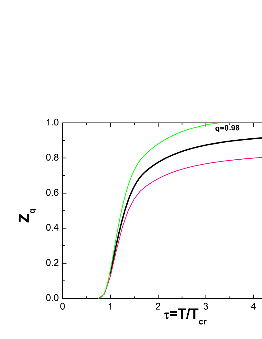
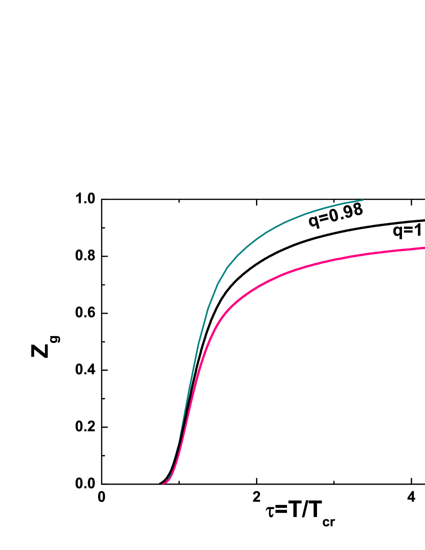
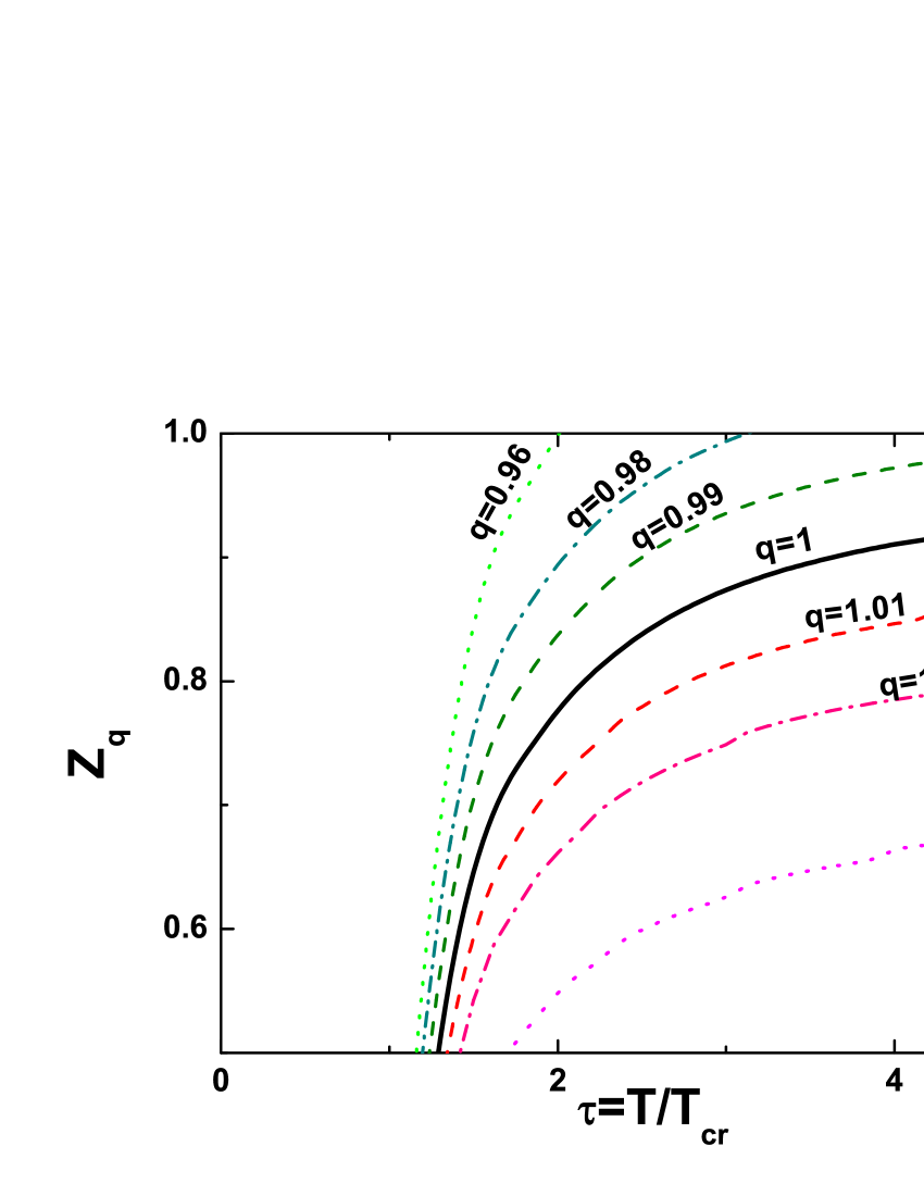
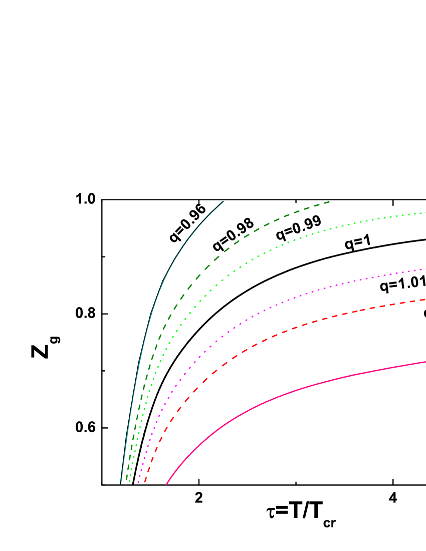
Figure 1: (Color online) Upper panels: Results for $z_{q}^{(q)}(\tau)$ and $z_{q}^{(g)}(\tau)$ as a function of the scaled temperature $\tau=T/T_{c}$ (calculated for $\mu=0$). Lower panels: As above but shown in more detail and with an enlarged range of the nonextensivity parameter $q$.

$$P_{q=1}(T)=P_{q}(T)$$ (18)

(it is tacitly assumed that in both extensive and nonextensive environments the temperature $T$ remains the same). This means that in our case the trace anomaly remains the same as in the $z$-QPM (and as in the lattice data) and does not depend on the nonextensivity. To this end the following conditions must be satisfied:

$$\int_{0}^{\infty}dpp^{2}\ln\left[1-e\left(-\tilde{x}^{(g)}\right)\right]=\int_{0}^{\infty}\,\,dpp^{2}\ln_{2-q}\left[1-e_{2-q}\left(-\tilde{x}_{q}^{(g)}\right)\right]\Theta\left(p;g)\right),$$ (19)

for gluons (with $\nu_{g}=16$) and

$$\nu_{q}\int_{0}^{\infty}dpp^{2}\ln\left[1+e\left(-\tilde{x}^{(q)}\right)\right]+\nu_{s}\int_{0}^{\infty}dpp^{2}\ln\left[1+e\left(-\tilde{x}^{(s)}\right)\right]=$$

$$=\nu_{q}\int_{0}^{\infty}dpp^{2}\ln_{2-q}\left[1+e_{2-q}\left(-\tilde{x}_{q}^{(q)}\right)\right]\Theta(p;q)+\nu_{s}\int_{0}^{\infty}dpp^{2}\ln_{2-q}\left[1+e_{2-q}\left(-\tilde{x}_{q}^{(s)}\right)\right]\Theta(p;s),$$ (20)

for quarks. They give us the $\tau$ and $q$-dependent relations between the extensive fugacities obtained in zQPM5 ), $z^{(i)}(\tau)$ (which are our input), and the nonextensive fugacities, $z_{q}^{(i)}(\tau)$ (which are our results). The function $\Theta(q,q)$ defines the allowed phase space; its details are presented in Appendix A.

Table 2: Numerical values of the coefficients $a_{(i)}$, $b_{(i)}$, $a^{\prime}_{(i)}$ and $b^{\prime}_{(i)}$ ($i=q,g$) in Eq. (6) when used for different values of $q$ resulting in the curves displayed in the lower panels of Fig. 1.

$q$	$(i)$	$a_{(i)}$	$b_{(i)}$	$a^{\prime}_{(i)}$	$b^{\prime}_{(i)}$
$q=0.96$	$i=g$	$0.985$	$1.581$	$1.168$	$0.860$
$q=0.96$	$i=q$	$1.030$	$1.510$	$1.200$	$0.747$
$q=0.98$	$i=g$	$0.897$	$1.702$	$1.078$	$0.870$
$q=0.98$	$i=q$	$0.924$	$1.603$	$1.073$	$0.770$
$q=0.99$	$i=g$	$0.850$	$1.760$	$1.028$	$0.904$
$q=0.99$	$i=q$	$0.867$	$1.662$	$1.018$	$0.799$
$q=1.01$	$i=g$	$0.753$	$1.916$	$0.927$	$0.990$
$q=1.01$	$i=q$	$0.751$	$1.791$	$0.896$	$0.879$
$q=1.02$	$i=g$	$0.704$	$2.006$	$0.876$	$1.059$
$q=1.02$	$i=q$	$0.694$	$1.862$	$0.835$	$0.925$
$q=1.04$	$i=g$	$0.600$	$2.221$	$0.766$	$1.180$
$q=1.04$	$i=q$	$0.580$	$2.061$	$0.712$	$1.050$

Figs. 1 shows the resulting effective fugacities, $z_{q}=z_{q}^{(q)}(\tau)$ and $z_{g}=z_{q}^{(g)}(\tau)$, as functions of the scaled temperature, $\tau=T/T_{c}$. They can be fitted using the same parametrization as before, i.e., Eq. (6), with the parameters displayed in Table II. Since the values of $z_{q=1}^{(i)}$ obtained in zQPM5 were obtained assuming $\mu=0$, the same assumption was used in obtaining our $z_{q}^{(i)}$ here. Note that for the nonextensivites $q$ used here the changes in the fugacities are small,

$$\delta z_{q}^{(q,g)}=z_{q}^{(q,g)}-z_{q=1}^{(q,g)}<1,$$ (21)

and can be approximated (with very good accuracy of a few percent) by (cf. Appendix B),

$$\delta z_{q}\simeq z_{q=1}(1-q)\cdot F\left(q=1,z_{q=1}\right)\quad{\rm where}\quad F=\frac{\int_{0}^{\infty}dpp^{2}\left\{\ln^{2}[1-\xi e(-x;z)]+n(x;z)x^{2}\right\}}{2\int_{0}^{\infty}dpp^{2}n(x;z)}.$$ (22)

Eq. (22), together with Fig. 1, allows for a better understanding of interrelation between the dynamics (represented by the fugacities $z$) and the nonextensivity described by $q$. The central point is that all the $z_{q}$ must describe the lattice QCD data (directly for $q=1$ in $z$-QPM and indirectly for $q\neq 1$ in $qz$-QPM, where they are forced to reproduce the results of $z$-QPM). The $\tau$-dependence of $z(\tau)$ starts from small values (corresponding to strong attraction) towards $z=1$ (corresponding to free, noninteracting particles). The case of $z>1$ would formally mean the emergence of repulsive forces and is not allowed in $z$-QPM, therefore we shall also keep this limitation in our $qz$-QPM. The replacement of extensive media by not extensive means adding some repulsive interaction (in the case of $q<1$) or an attractive one (for $q>1$). Therefore, in the first case it must be compensated by an increase in $z$ (i.e., $\delta z_{q}>0$) and in the second case by a decrease (i.e., $\delta z_{q}<0$). Note now that whereas in the latter case we have $z_{q}(\tau)<z_{q=1}(\tau)<1$, in the former there is limiting value of $\tau=\tau_{lim}(q)$, depending on $q$, for which $z_{q}\left(\tau_{lim}\right)=1$. This means that for $\tau>\tau_{lim}(q)$ the attraction represented by $z(\tau)$ is already too weak to compensate the repulsion introduced by $q<1$. The value of $\tau_{lim}$ diminishes with the increase of this repulsion (i.e., with the increase of $|q-1|$). Not wanting to introduce the problem of repulsion we limit our considerations to $\tau>\tau_{lim}$ only.

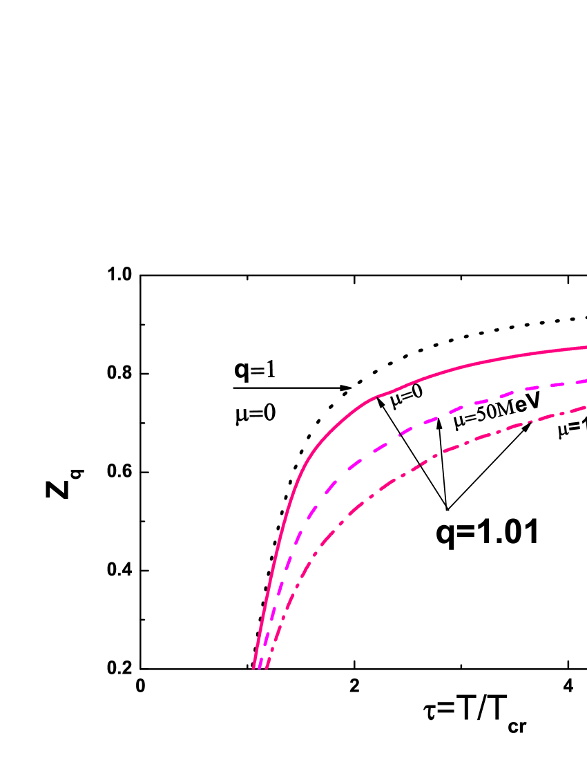
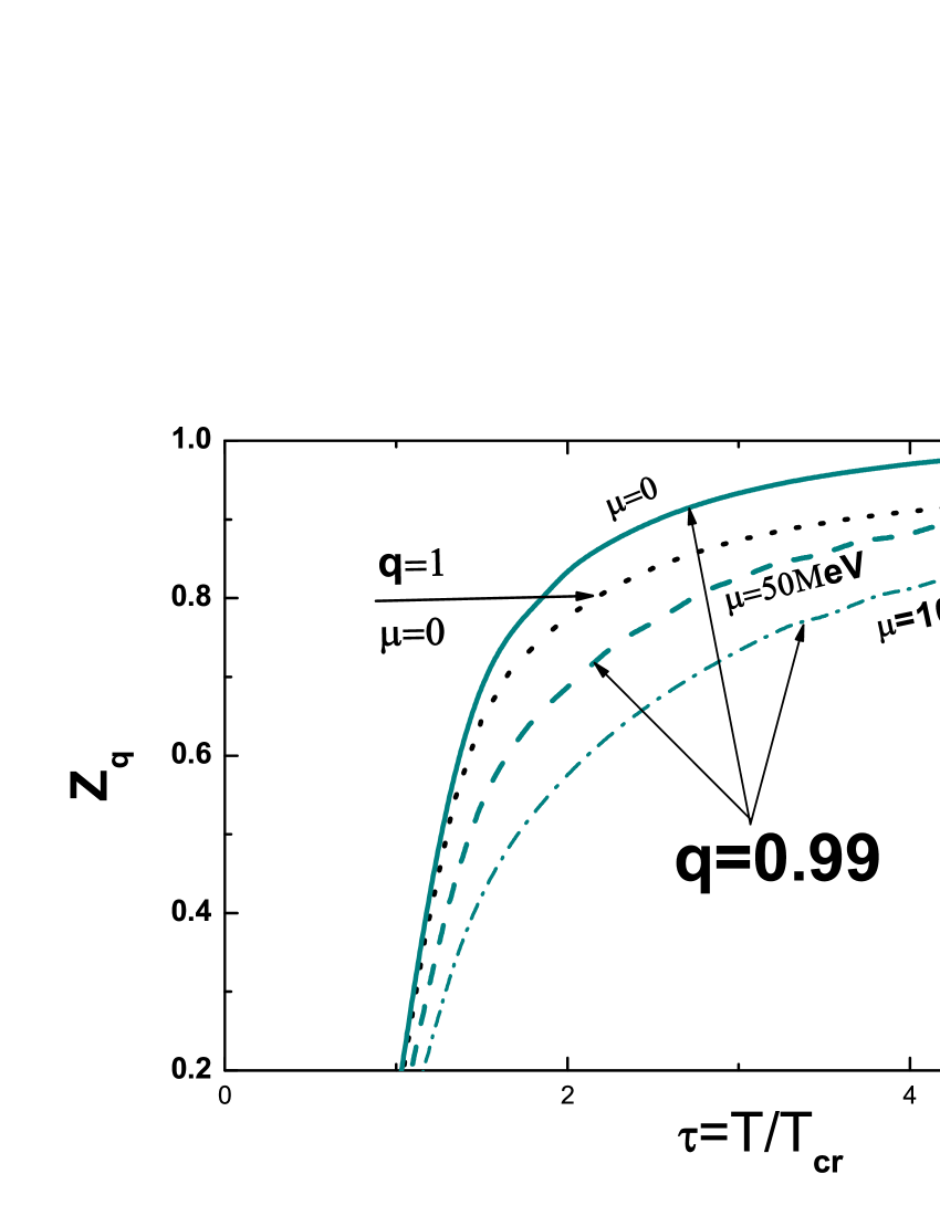
Figure 2: (Color online) Illustration of the changes introduced by the chemical potential $\mu$ for $q=1.01$ and $q=0.99$.

So far, results for $z(\tau)$ and $z_{q}(\tau)$ have been obtained with $\mu=0$. The formal introduction of the chemical potential $\mu$ in $z$-QPM zQPM12 makes $z$-QPM more flexible and applicable to possible future lattice QCD data with the chemical potential accounted for. Following this new development in $z$-QPM we have also formally introduced $\mu$ into our $z$-QPM. We can therefore check what would be the value of our $z_{q}$ in the case when part of the dynamics is shifted from fugacity $z$ to the chemical potential $\mu$. Eq. (5) shows the effective fugacity with the chemical potential included. It is visualized in Fig. 2 where we plot a number of results for different values of the chemical potential $\mu$ and for two values of the nonextensivity parameter: $q=0.99$ and $q=1.01$. As one can see, nonzero $\mu$ diminishes the real values of the fugacity because, according to Eq. (5) (valid also in a nonextensive environment with $\tilde{z}\to\tilde{z}_{q}$), the effective value $\tilde{z}_{q}$ now contains an exponential factor greater than unity, which modifies the original fugacity $z$.

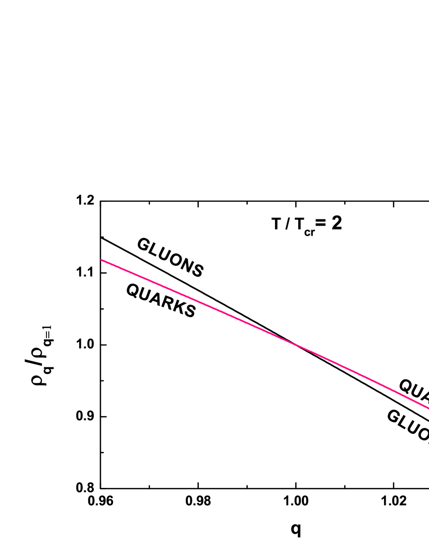
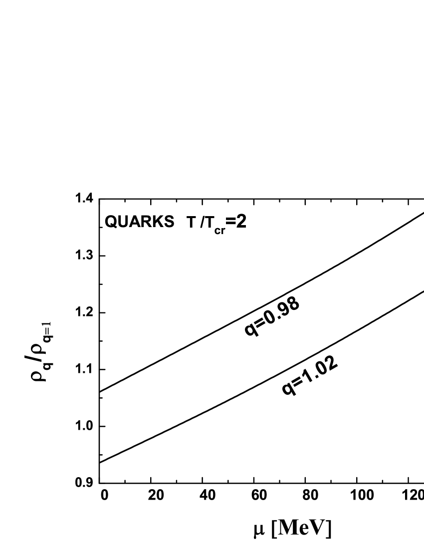
Figure 3: (Color online) Left panel: Relative density, $\rho_{q}/\rho_{q=1}$, of quarks and gluons as a function of the nonextensivity $q$ for $\mu=0$. Right panel: Dependence of the relative density, $\rho_{q}/\rho_{q=1}$, on the chemical potential $\mu$.

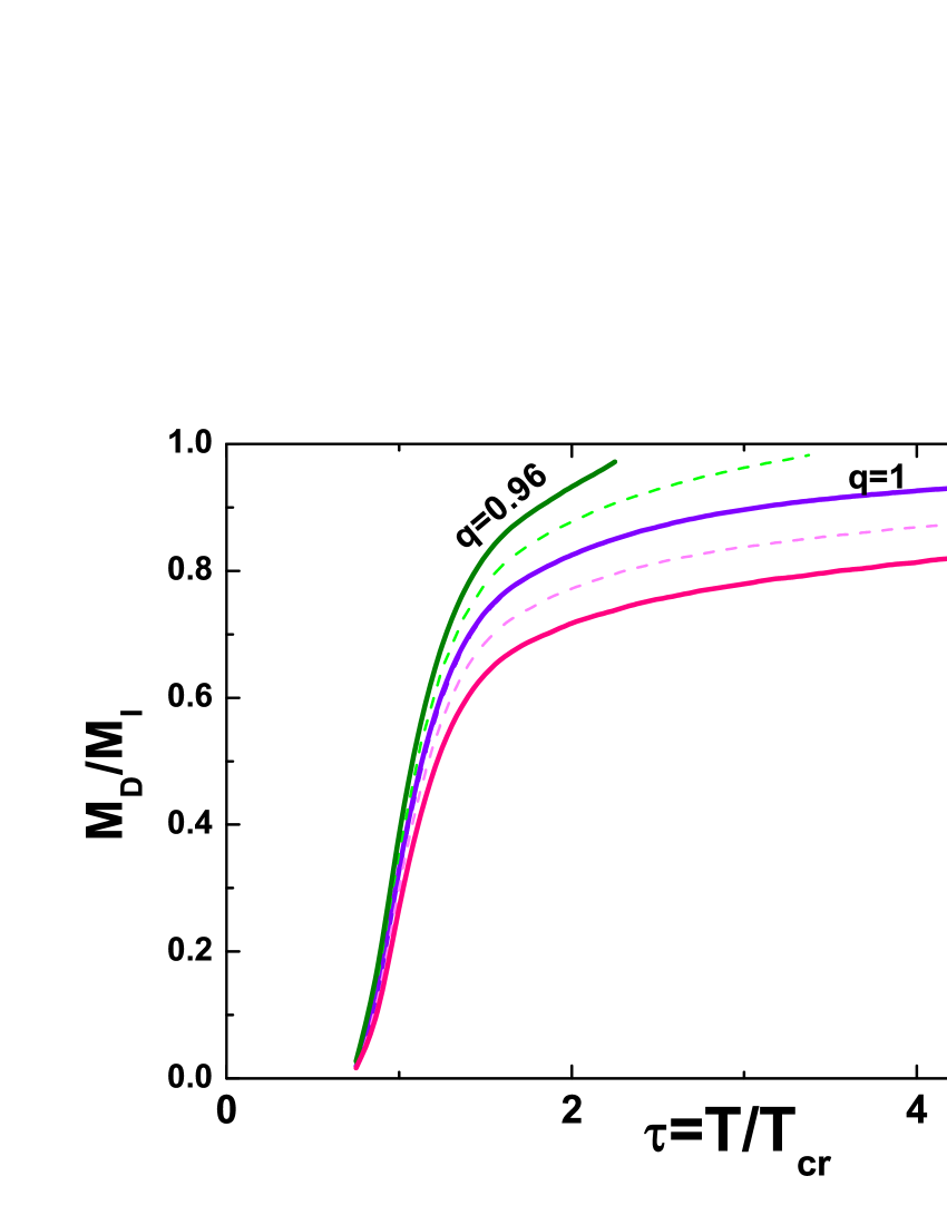
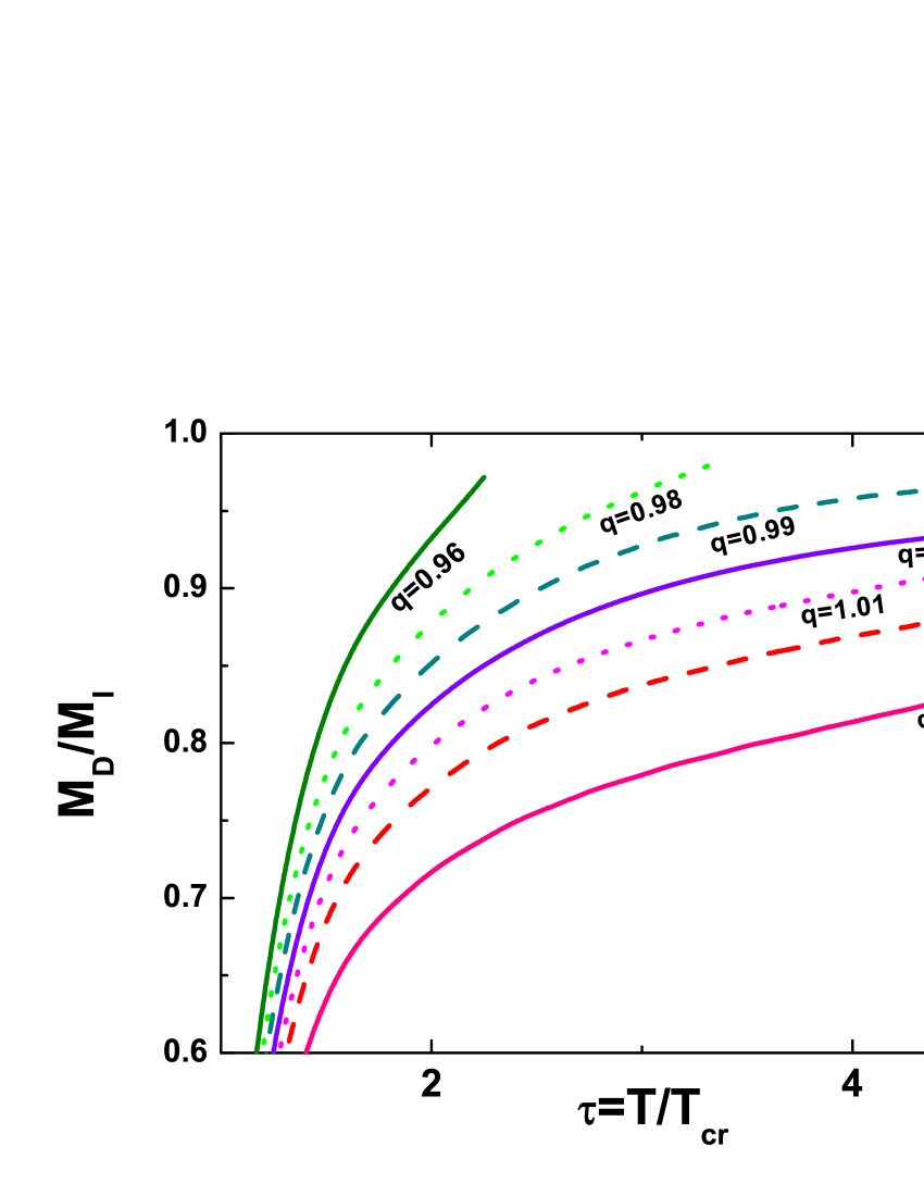
Figure 4: (Color online) Left panel: Results for the ratio $M_{D}/M_{D}^{I}$ of the Debye masses (as defined by Eqs. (23) and (24)), respectively) in the nonextensive environment as functions of the scaled temperature, $\tau=T/T_{c}$ for $q=0.96,~{}1,~{}1.04$, calculated for $\mu=0$. Right panel: The same as above but shown in more detail and with an enlarged range of the nonextensivity parameter $q$.

The introduction of the chemical potential $\mu$ also changes the $q$-dependence of the relative density of the quarks, $R_{\rho}=\frac{\rho_{q}}{\rho_{q=1}}$, where $\rho_{q}$ is given be Eq. (13). As can be seen in the left panel of Fig. 3, in a nonextensive environment one observes a clear separation of the situations with $R_{\rho}>1$ and $R_{\rho}<1$. The first occurs for $q<1$ and the observed increase of density is consistent with lowering of the entropy which, in turn, is connected with the tighter packing of the quarks in this case JRGW . The second occurs for $q>1$ and the picture is reversed; it is consistent with an increase of the entropy and with looser packing of the quarks in this case. Note that this behaviour of $R_{\rho}=R_{\rho}(q)$ is fully consistent with the behaviour of the nonextensive fugacities presented in Fig. 1. Essentially the same result can be obtained using the linear approximation of the $n_{q}^{q}$ in $(q-1)$ as given by Eqs. (59) and (59). Using now the same values of $z_{q}$ but adding some amount of the chemical potential $\mu$ yields the results shown in the right panel of Fig. 3. We observe some increase of the relative density with $\mu$ with a possible trace of a small upper bending.

We shall now calculate the modifications of partonic charges in a hot QCD medium embedded in a nonextensive environment calculating the corresponding Debye mass, $M_{qD}$. Following zQPM5 we use for the extensive Debye mass the expression derived in semiclassical transport theory in which $M_{D}$ is given in terms of equilibrium parton distribution functions ($N_{c}$ denotes the number of colors):

$$M^{2}_{D}=-2N_{c}Q^{2}\int\frac{d^{3}p}{8\pi^{3}}\partial_{p}n^{(g)}-Q^{2}\int\frac{d^{3}p}{8\pi^{3}}\partial_{p}\left(4n^{(q)}+2n^{(s)}\right)=\frac{N_{c}Q^{2}}{\pi^{2}}n^{(g)}-Q^{2}\left(2n^{(q)}+n^{(s)}\right).$$ (23)

In the nonextensive environment described by the nonextensivity parameter $q$ we simply replace $n^{(i=g,q,s)}(x;z)$ by $\left[n_{q}^{(i)}\left(x;z_{q}\right)\right]^{q}$. In Fig. 4, following zQPM5 , we present the ratio of $M_{D}/M_{D}^{I}$ where $M_{D}^{I}$ denotes the Debye mass for the ideal EOS case (i.e., with $z_{g}=1$ and $z_{q}=1$) which, following zQPM5 , equals

$$M_{D}^{I}=QT\sqrt{\frac{N_{c}}{3}+\frac{1}{2}-\frac{m^{2}}{4\pi^{2}T^{2}}\ln 2}.$$ (24)

Note that because the Debye mass is essentially a combination of the densities of quarks and gluons the above results resemble those for the effective fugacities and all previous remarks also apply here.

We now proceed to the second part of our work in which we keep the original dynamics of the $qz$-QPM intact using the same effective fugacities as in zQPM5 (i.e., we assume that $z_{q}{(i)}\to z^{(i)}$ as given by Eq. (6) with the parameters listed in Table I). This parallels to some extent our approach in the nonextensive $q$-NJL model JRGW (but now the dynamics is simplified and represented by the temperature dependent fugacities $z(\tau)$ reproducing the lattice QCD results) and allows us to investigate the sensitivity of the selected observables to the nonextensive environment only. The only drawback is the limitations in the temperatures allowed because the fugacities are only defined for $\tau>1$, i.e., above the critical temperature $T_{c}$.

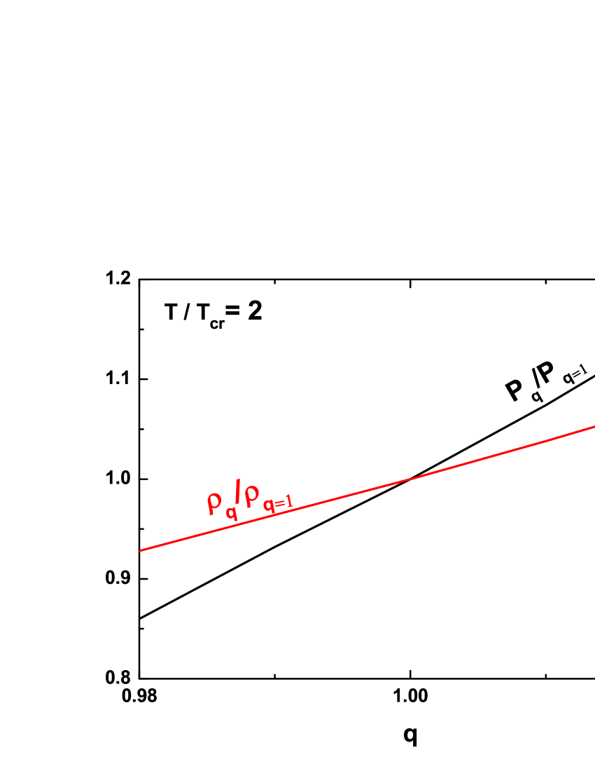
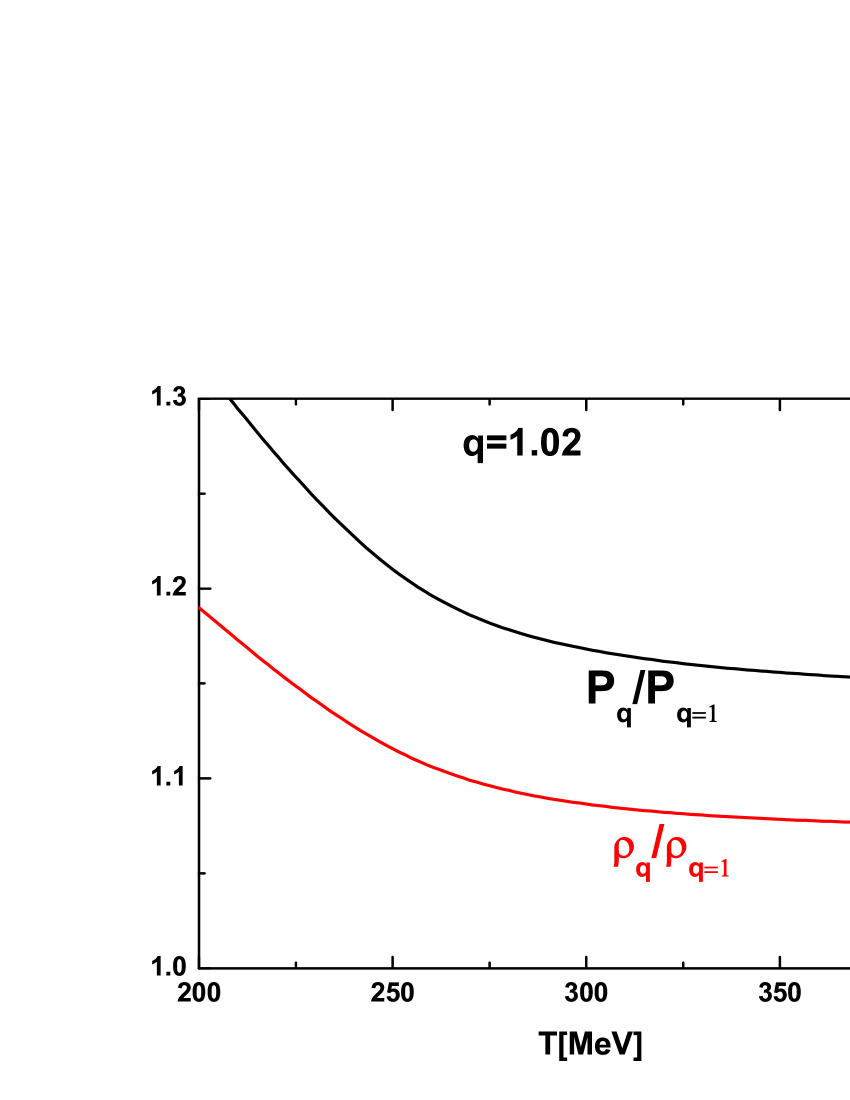
Figure 5: (Color online) Dependencies of relative pressure $P_{q}/P_{q=1}$ and density $\rho_{q}/\rho_{q=1}$ on the nonextensivity parameter $q$ at fixed temperature (left panel) and on the temperature $T$ for fixed $q$ (right panel).

To start with we present in Fig. 5 the corresponding relative pressure $P_{q}/P_{q=1}$ and relative density $\rho_{q}/\rho_{q=1}$ as functions of the nonextensivity parameter $q$ at fixed temperature (left panel) and their dependencies on $T$ for some fixed nonextensivity $q$ (right panel). Note that whereas before the pressure was assumed to be the same for extensive and nonextensive environments, $P_{q}/P_{q=1}=1$, it now increases linearly with $q$ in the same way as in the $q$-NJL model JRGW . The relative density also increases with the nonextensivity $q$, contrary to its previous behaviour (demonstrated in the left panel of Fig. 3) where it decreased with $q$.

We now proceed to the trace anomaly, $\mathbb{T}_{q}$, Eq. (17). Note that now it acquires some explicit dependence on the nonextensive parameter $q$. Using the definitions of energy density, $\varepsilon_{q}$, Eq. (14) and pressure $P_{q}$ (Eq. (16) (and additionally Eqs. (3) and (4)), we obtain that

$$\mathbb{T}_{q} = \beta^{4}\int\frac{d^{3}p}{(2\pi)^{3}}\sum_{i}\nu_{i}\left[E_{i}-p\frac{\partial\tilde{x}^{(i)}}{\partial p}-\frac{\partial}{\partial\beta}\ln z^{(i)}(\beta)\right]\cdot\left[n_{q}\left(\tilde{x}^{(i)}\right)\right]^{q}=$$ (25)

$$= -\beta^{4}\frac{\partial}{\partial\beta}\ln z^{(i)}(\beta)\cdot\int\frac{d^{3}p}{(2\pi)^{3}}\sum_{i}\nu_{i}\left[n_{q}\left(\tilde{x}^{(i)}\right)\right]^{q}.$$

The change in the trace anomaly generated by the nonextensivity $q$ is given by (see Eqs. (59) and (59))

$$\Delta\left[\mathbb{T}_{q}\right] = \mathbb{T}_{q}-\mathbb{T}_{q=1}=-\beta^{4}\frac{\partial}{\partial\beta}\ln z^{(i)}(\beta)\cdot\int\frac{d^{3}p}{(2\pi)^{3}}\sum_{i}\nu_{i}\Delta^{(i)}\left[n^{q}_{q};n\right];$$ (26)

$$\!\!\!\!\!\Delta^{(i)}\left[n^{q}_{q};n\right]\!\! = \!\!\left\{\left[n_{q}\left(\tilde{x}^{(i)}\right)\right]^{q}-\left[n\left(\tilde{x}^{(i)}\right)\right]\right\}\simeq$$ (27)

$$\simeq (q-1)n\left(\tilde{x}^{(i)}\right)\left\{\ln n\left(\tilde{x}^{(i)}\right)+\frac{1}{2}\left[1+\xi n\left(\tilde{x}^{(i)}\right)\right]\left(\tilde{x}^{(i)}\right)^{2}\right\}.$$

Fig. 6 shows the dependence of the trace anomaly on the nonextensivity $q$ (left panel) and chemical potential $\mu$ (right panel). Note that for large values of the scaled temperature $\tau$ the effects caused by the nonextensivity and by the chemical potential gradually vanish.

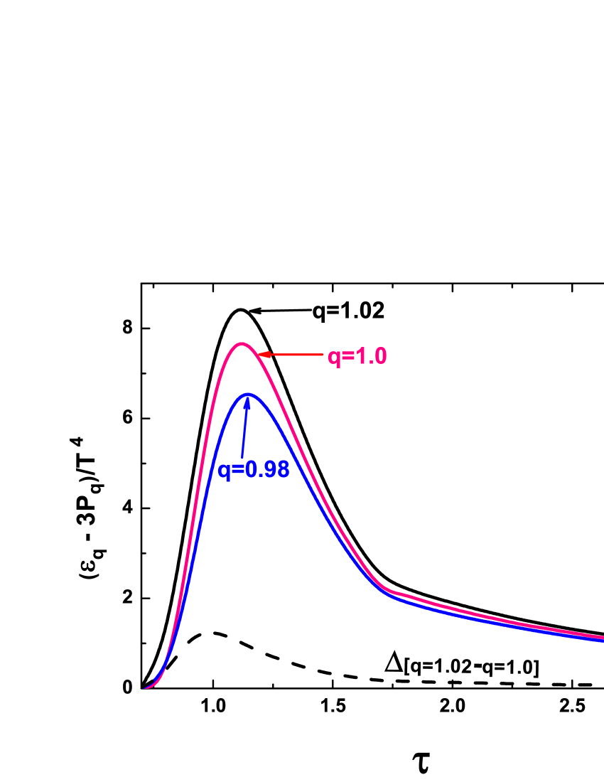
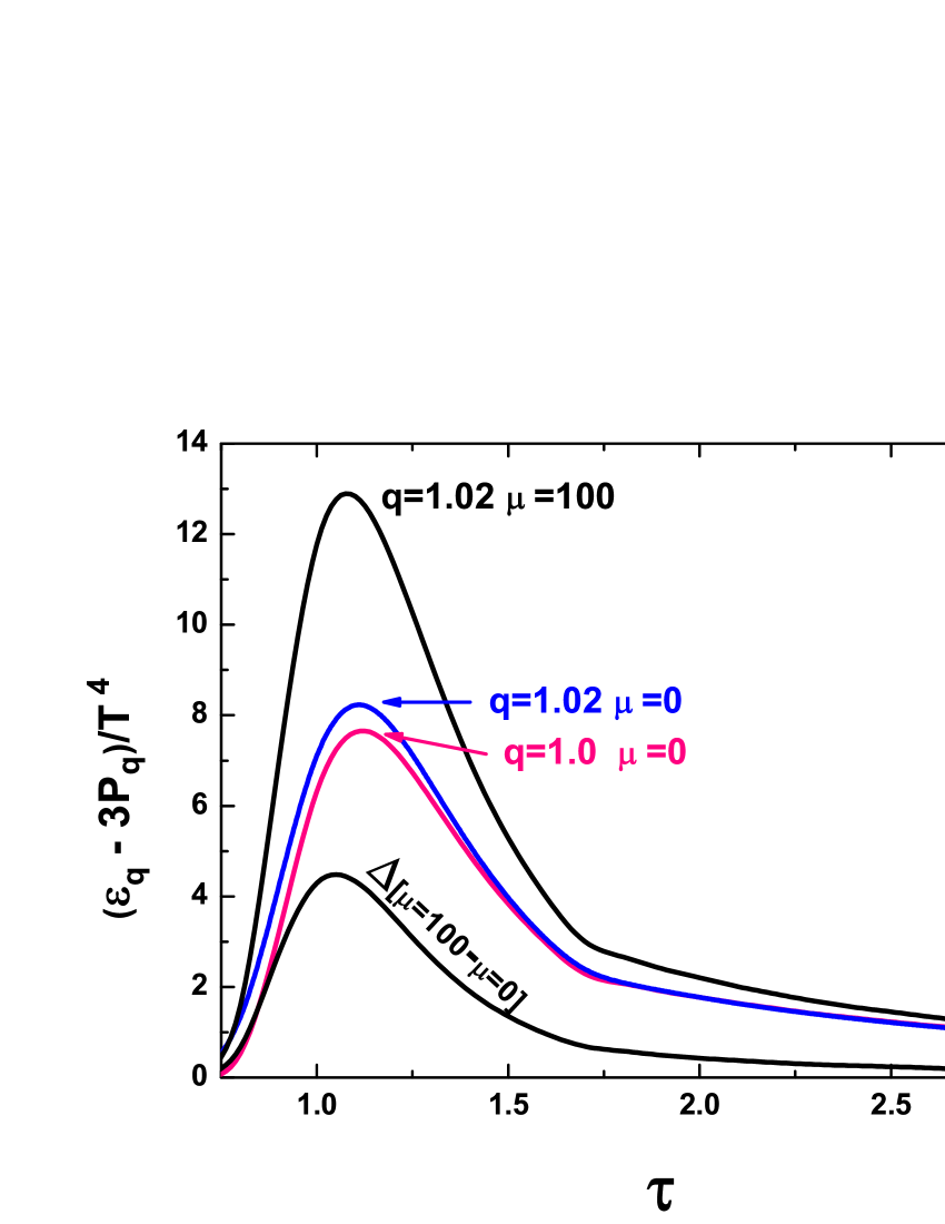
Figure 6: (Color online) The behaviour of the change in the trace anomaly in the $qz$-QPM with $z_{q}=z_{q=1}$ as a function of $\tau$ for some selected values of $q$ (left panel) and the same but for some selected values of the chemical potential $\mu$ (right panel).

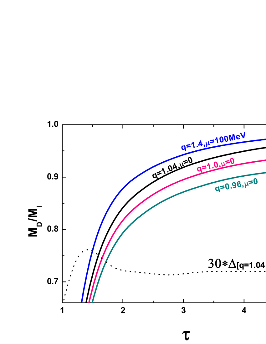
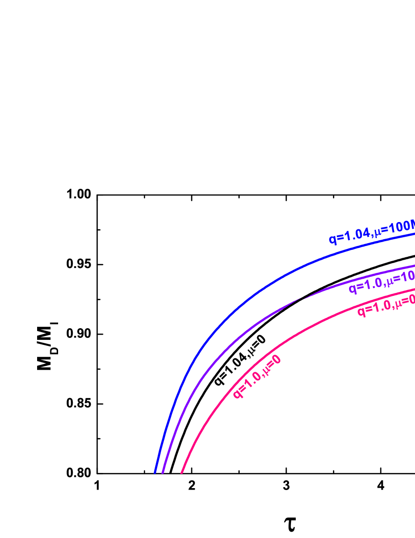
Figure 7: (Color online) The behaviour of the ratio $M_{D}/M_{D}^{I}$ of the Debye masses (as defined by Eqs. (23)) and (24) as a function of $\tau$ for some selected values of $q$ (left panel) and the same but for some selected values of the chemical potential $\mu$ (right panel). The dynamics is the same as in the $z$-QPM, i.e., $z_{q}=z_{q=1}=z$.

In Fig. 7 we present the $\tau$ dependence of the ratio $M_{D}/M_{D}^{I}$ of the Debye masses (as defined by Eqs. (23)) and (24) for different nonextensivities $q$ (left panel) and chemical potentials $\mu$ (right panel). Unlike the results presented in Fig. 4, this time they are caused solely by the action of the nonextensive environment with $z_{q}=z_{q=1}=z$ as used in the $z$-QPM.

5 Summary and conclusions

In this work we investigate the interrelation between nonextensive statistics and the effects of dynamics in dense QCD matter. It continues our previous analysis of this problem on the example of the nonextensive version of the NJL model, the $q$-NJL. However, the complexity of its dynamics does not allow for a clear separation of the purely dynamical effects from the nonextensive ones. Therefore, in this work, following some specific quasi-particle models ($z$-QPM) zQPM5 ; zQPM6 ; zQPM6a ; zQPM11a ; zQPM12 ; zQPM14 , we used simplified dynamics reduced to a number of well defined parameters, the effective fugacities, $z\in(0,1)$. In this kind of QPM the masses of the quasi-particles are not modified by the interaction, which enables the problems and inconsistencies encountered in other approaches to be avoided. The fugacities $z$ increase with temperature $T$ from very small values in the vicinity of the critical temperature, $T_{cr}$ (which corresponds to strong interactions between quarks and gluons), towards unity (which corresponds to a free gas of quarks and gluons). They modify only the argument of the exponent in the corresponding Bose-Einstein or Fermi-Dirac distributions: $e(x)\to e(x-\ln z)$. The action of nonextensivity is different, it changes the functional form of the exponent, $e(x)\to e_{q}(x)$, leaving the argument $x$ unchanged. This means that the actions of nonextensivity and dynamics are complementary and cannot be replaced by each other (although sometimes they describe the same, or comparable, situations). The fugacity $z$ therefore models phenomenologically the dynamics of the mean field theory in the extensive environment and does not account for intrinsic correlations and fluctuations present in the system, while these are most naturally described phenomenologically by the nonextensivity $q$. Phenomenologically, both approaches nicely complement each other in what concerns the description of the dense QCD system. If we wanted to replace the action of nonextensivity, $q$, by the respective action of dynamics, $z$, (or vice versa) then either $z$ or $q$ would have to acquire energy dependence, which we consider as untenable.

Note that, contrary to the $q$-NJL model JRGW , the $qz$-QPM model is formulated in such a way as to reproduce the effective fugacities of the original $z$-QPM zQPM5 , which, in turn, describes the lattice QCD results Latt-mu1 ; Latt-mu3 . This means that the $qz$-QPM also describes them; in fact they serve as a kind of experimental data. Such constraints were not present in the $q$-NJL model. Therefore, our conclusions are more reliable than those presented in JRGW . The interplay between dynamics and nonextensivity is best seen in Fig. 3 (left panel) which shows results for the relative densities, $R_{\rho}=\rho_{q}/\rho_{q=1}$, in the nonextensive environment. For $q<1$ (which corresponds to a lowering of the entropy) one observes $R_{\rho}>1$, which can be interpreted as caused by some positive (attractive) correlations in the system and may be connected with a tighter packing of quarks. The opposite is observed for $q>1$ (corresponding to an increase of the entropy) where $R_{\rho}<1$. This can be interpreted as resulting from the repulsion of the quarks and fluctuations developing in the system. Both of these correlations and fluctuations are imposed on the effects of the interaction described by the fugacities $z_{q}$. This is the clearest example of dynamical effects introduced by the nonextensive environment and characterized by the nonextensivity parameter $q$.

Let us now look more closely at the results on $z_{q}(\tau)$ presented in Fig. 1. Note that for $q<1$, when, according to the left panel of Fig. 3 our system becomes more dense, one observes that $\delta z_{q}=z_{q<1}-z_{q=1}>0$ and increases with $|q-1|$ (i.e., increases with density). This means that the interaction represented by $z_{q}$ becomes weaker. As a result, the upper limit of $z_{q}=1$ (corresponding to a noninteracting gas of quarks and gluons) is reached for smaller temperature $T$, the more so the bigger $|q-1|$ (i.e., the smaller $q$). This means that to obtain the same pressure in the system one needs a weaker interaction described by fugacity; the increasing part of it is caused by the effect of the nonextensivity $q$. In other words: the change of statistics from extensive ($q=1$) to nonextensive with $q<1$, allows the attainment of the limit of the ideal gas with weaker correlations between quarks and gluons caused by the fugacity $z$. For the $q>1$ case our system becomes, according to the left-panel of Fig. 3, less dense; the correction term needed to obtain the same pressure as in the extensive case is now negative, $\delta z_{q}=z_{q>1}-z_{q=1}<0$, and $|\delta z_{q}|$ grows only very slowly with increasing $q$ (i.e., with decreasing density) becoming constant for higher $T$; the limit $z_{q}=1$ is never reached for finite temperature $T$. This is because for $q>1$ one expects some intrinsic fluctuations (for example temperature $T$ fluctuations) which work against the dynamical interactions represented by $z$. Therefore, these interactions cannot cease and $z_{q}$ cannot grow too fast. In fact, with increasing $T$ they seem to become constant and one observes a kind of equilibrium between dynamics and nonextensivity.

Because the $z$-QPM zQPM5 ; zQPM6 ; zQPM6a ; zQPM11a ; zQPM12 ; zQPM14 uses the lattice QCD results LQCD1 ; LQCD3 ; LQCD4 as its input and because there are problems with nonzero chemical potential $\mu$ in the lattice calculations Latt-mu1 ; Latt-mu3 , the $z$-QPM was initially formulated for zero chemical potential, $\mu=0$, which substantially limits its applications. However, anticipating the possibility of the emergence of some new lattice QCD results with the chemical potential included (if only partially), starting from zQPM12 some small amount of non-vanishing $\mu$ in the matter sector was introduced. We have therefore also allowed for some nonvanishing $\mu$. In Fig. 2 we show how nonzero $\mu$ influences the extracted $z_{q}$ for $q<1$ and $q>1$. Fig. 3 (right panel) shows that the relative density (both for $q<1$ and $q>1$) increases (almost) linearly with the chemical potential. Note that the possible introduction of the chemical potential in the lattice QCD calculations will change profoundly the $z$-QPM (and the $qz$-QPM); it will therefore become a third phenomenological parameter modelling the interaction. Our results shows in what direction these changes will proceed and in Appendix D we provide a scheme of expansion of the pressure in the chemical potential to allow for the possible further application of our $qz$-QPM should similar results occur in the lattice calculations Latt-mu1 ; Latt-mu3 .

Fig. 4 presents the results for the Debye mass in a nonextensive environment. Note that because it is essentially a combination of densities of quarks and gluons the results therefore resemble those for the effective fugacities. Calculations of more involved quantities, like, for example, dissipative effects would be much more involved because they would demand the use of the nonextensive version of the transport or hydrodynamic equations, which is beyond the scope of this work and will be presented elsewhere. It would also be desirable to be able to compare directly the results of $qz$-QPM with some future nonextensive lattice QCD simulations, which seems to be gaining some interest recently qLatt ; qLatt1 .

Finally, Figs. 5 - 7 present some selected results on the, respectively, relative pressure and density, trace anomaly and Debye mass obtained when we use the $qz$-QPM with the same effective fugacities $z^{(i)}$ as in the $z$-QMP and calculate changes in densities and pressure induced only by changes in the nonextensivity $q$. Because in this case the original dynamics represented by $z^{(i)}$ remains intact, all changes in the results are caused only by the nonextensivity, i.e., by the fact that $|q-1|\neq 0$. These results correspond, in a sense, to the results obtained in our $q$-NJL model JRGW , with the proviso that now our investigations are limited to $T$ above the critical temperature $T_{c}$ (i.e., to $\tau=T/T_{c}>1$ because only such are considered in $z$-QMP). In both models we observe similar dependencies of the pressure and density on the nonextensivity parameter $q$ while maintaining all dynamical parameters for a given temperature $T$ the same. They are reduced for $q<1$ and enhanced for $q>1$. This means that when changing the amount of nonextensivity one cannot keep the same pressure $P$ in the system without changing the dynamical parameters (or their temperature dependencies). Our $qz$-QPM is therefore a simple example of such changes needed to achieve equalization of the pressure in extensive and nonextensive systems. Note that now, as a result of the pressure equalization in extensive and nonextensive systems, the relative densities, $R_{\rho}=\rho_{q}/\rho_{q=1}$, change with $q$ in opposite ways, becoming higher for $q<1$ and lower for $q<1$ than the density in an extensive system. This observation could be important for some new version of the $q$-NJL model, in which one could insist on keeping the same pressure for different nonextensivities and looking for the corresponding changes in its dynamical parameters (which would become $q$-dependent). Such an approach could have its further application in investigations of the EoS of dense matter.

Appendix A Limitations of the allowed phase space in the nonextensive approach

The functions $\Theta(p;i)$ ($i=g$ for gluons, $i=q$ for light quarks and $q=s$ for strange quarks) provide the limitations of the allowed phase space resulting from the condition

$$[1+(q-1)x]\geq 0,$$ (28)

In the $q<1$ case, for gluons (with zero mass and zero chemical potential) we have that

$$\tilde{x}^{(i)}<\frac{1}{1-q}\qquad\Longrightarrow\qquad\frac{p}{T}<\frac{1}{1-q}+\ln z_{q}^{(g)}.$$ (29)

Because $z_{q}^{(g)}<1$, our integral is non-vanishing (i.e., $p>0$) only for

$$\frac{1}{1-q}+\ln z_{q}^{(g)}>0\quad\Longrightarrow\quad z_{q}^{(g)}>e\left(-\frac{1}{1-q}\right).$$ (30)

Stronger interactions (corresponding to smaller values of the fugacity) are in this case not allowed for the $q$ used here. In the case of quarks (with chemical potential $\mu>0$ and with mass $m$ for strange quarks) condition (29) results in the following limitation

$$\frac{\sqrt{p^{2}+m^{2}}}{T}<\frac{1}{1-q}+\frac{\mu}{T}+\ln z_{q}^{(i)},\quad(i=q,s).$$ (31)

Now the phase space is open if:

$$\frac{1}{1-q}+\frac{(\mu\pm m)}{T}+\ln z_{q}^{(i)}>0\qquad{\rm or}\qquad\frac{1}{1-q}+\frac{(\mu\pm m)}{T}+\ln z_{q}^{(i)}<0.$$ (32)

In the first case the $(\mu-m)$ choice is more restrictive and results in the condition that

$$z_{q}^{(i)}>e\left(-\frac{1}{1-q}\right)\cdot e\left(-\frac{\mu-m}{T}\right),$$ (33)

which for $\mu=0$ and $m=0$ coincides with the corresponding condition for gluons. In the second case the choice $(\mu+m)$ is the more restrictive, for which

$$z_{q}^{(i)}>e\left(-\frac{1}{1-q}\right)\cdot e\left(-\frac{\mu+m}{T}\right).$$ (34)

For nonzero mass (strange quarks) it is more restrictive than condition (33).

In the case of $q>1$ we have for gluons that

$$x^{(i)}>-\frac{1}{q-1}\qquad\Longrightarrow\qquad\frac{p}{T}>\ln z_{q}^{(g)}-\frac{1}{q-1}.$$ (35)

In our case it is always satisfied and there are no limitations on $z_{q}^{(g)}$. The same situation is now in the quark sector and there are also no limitations $z_{q}^{(i)}$. For gluons, which are bosons, one has an additional condition, namely

$$e_{q}(x)>1\quad\Longrightarrow\quad p>T\ln z_{q}^{(i)}\quad{\rm for~{}all}\quad q.$$ (36)

However, for $z_{g}<1$ it does not introduce any further limitations.

Appendix B Approximate calculation of $z_{q}$

Let us denote $z_{q}=z+\delta$ (where $z=z(\tau)$ are the fugacities obtained in zQPM5 from lattice QCD and $\delta=z_{q}-z$ is the change in fugacity emerging from the nonextensive environment). We shall now calculate $\delta/z$ for the case of small $\delta$, $|\delta/z|<<1$. We start by expanding $L_{q}(x)$ from Eq. (11),

$$L_{q}\left(x_{q};\delta\right)=\ln_{2-q}\left[1-\xi e_{2-q}\left(-x_{q}\right)\right]=\ln_{2-q}(X),$$ (37)

in $\delta$ and keeping only linear terms:

$$L_{q}\left(x_{q};\delta\right)\simeq L_{q}\left(x_{q};\delta=0\right)+\frac{\partial L_{q}\left(x_{q};\delta\right)}{\partial\delta}\bigg{|}_{\delta=0}\cdot\delta.$$ (38)

Denoting

$$X=1-\xi E,\quad E=e_{2-q}\left(-x_{q}\right),\quad x_{q}=y-\ln z_{q},$$ (39)

one can write that (cf., Eqs. (8) and (7))

$$\frac{\partial L_{q}\left(x_{q};\delta\right)}{\partial\delta} = \frac{\partial L_{q}(X)}{\partial X}\cdot\frac{\partial X}{\partial E}\cdot\frac{\partial E}{\partial x_{q}}\cdot\frac{\partial x_{q}}{\partial z_{q}}\cdot\frac{\partial z_{q}}{\partial\delta},$$ (40)

$$\frac{\partial L_{q}(X)}{\partial X} = \frac{\partial\ln_{2-q}(X)}{\partial X}=X^{-q},$$ (41)

$$\frac{\partial X}{\partial E} = -\xi,\qquad\frac{\partial E}{\partial x_{q}}=-\left[e_{2-q}(-x_{q})\right]^{q},\qquad\frac{\partial x_{q}}{\partial z_{q}}=-\frac{1}{z_{q}},\qquad\frac{\partial z_{q}}{\partial\delta}=1$$ (42)

obtaining (note that for $\delta=0$ $x_{q}\to x-\ln z$)

$$\!\!\!\!\!\frac{\partial L_{q}\left(x_{q};\delta\right)}{\partial\delta}\bigg{|}_{\delta=0}\!=\!-\frac{\xi}{z}\left[n_{q}(x;z)\right]^{q}\quad{\rm and}\quad L_{q}\left(x_{q};\delta\right)\simeq\ln_{2-q}\left[1-e_{2-q}\left(-x;z\right)\right]-\frac{\xi}{z}\left[n_{q}\left(x;z\right)\right]^{q}\delta.$$ (43)

The integrals of the type presented in Eqs. (19) and (20) can therefore be rewritten as integrals over

$$\Delta L_{q} = L(x;z)-L_{q}(x;\delta)=\ln[1-e(-x;z)]-\ln_{2-q}\left[1-\xi e_{2-q}\left(-x_{q};z_{q}\right)\right]\simeq$$ (44)

$$\simeq \left\{\ln[1-e(-x;z)]-\ln_{2-q}\left[1-\xi e_{2-q}(-x;z)\right]\right\}+\xi\left[n_{q}(x;z)\right]^{q}\cdot\frac{\delta}{z}=$$

$$=\left[I(x;z)-I_{q}(x;z)\right]+\xi\left[n_{q}(x;z)\right]^{q}\cdot\frac{\delta}{z}.$$

Because $z_{q}$ is obtained from the condition that $\Delta L_{q}=0$, in the first approximation the correction term $\delta$ is equal to

$$\delta = \xi z\cdot\frac{\int_{0}^{\infty}dpp^{2}\left[I(x;z)-I_{q}(x;z)\Theta(p)\right]}{\int_{0}^{\infty}dpp^{2}\left[n_{q}(x;z)\right]^{q}\Theta(p)}.$$ (45)

$\Theta(p)$ represents the possible limitation of the phase space caused by the nonextensivity (cf. Appendix A). It depends on the nonextensivity parameter $q$ and on the type of particle considered (gluons, light quarks or strange quarks).

Formula (45) can be further approximated by expanding it in $q-1$ and retaining only the linear terms in $(q-1)$. Following Eqs. (67) and (68) one obtains that

$$I_{q}(x;z)\simeq I(x;z)+\frac{1}{2}(q-1)\Delta I(x;z)\quad{\rm where}\quad\Delta I(x;z)=-\ln^{2}[1-\xi e(-x)]+n(x;z)x^{2}.$$ (46)

Similarly, following Eqs. (59) and (59), one has that

$$n_{q}^{q}\simeq n(x;z)+(q-1)n(x;z)\Delta_{q}[n(x;x)]\quad{\rm where}\quad\Delta_{q}[n(x;z)]=\ln n(x;z)+\frac{1}{2}[1+\xi n(x;z)]x^{2}.$$ (47)

Therefore

$$\xi\frac{\delta}{z}=\frac{A(x;z)-(q-1)B(x;z)}{C(x;z)+(q-1)D(x;z)}\simeq\frac{A(x;z)}{C(x;z)}-(q-1)\left\{\frac{B(x;z)}{C(x;z)}+\frac{A(x;z)D(x;z)}{[C(x;z)]^{2}}\right\},$$ (48)

where

$$A(x;z) = \int_{0}^{\infty}dpp^{2}I(x;z)[1-\Theta(p)],$$ (49)

$$B(x;z) = \frac{\xi}{2}\int_{0}^{\infty}dpp^{2}\Delta I(x;z)\Theta(p),$$ (50)

$$C(x;z) = \int_{0}^{\infty}dpp^{2}n(x;z)\Theta(p),$$ (51)

$$D(x;z) = \int_{0}^{\infty}dpp^{2}\Theta(p)n(x;z)\cdot\left\{\ln n(x;z)+\frac{1}{2}[1+\xi n(x;z)]x^{2}\right\}.$$ (52)

In practical applications it turns out that $A(x;z)\simeq 0$, therefore

$$\frac{\delta}{z}\simeq-\xi\cdot(q-1)\frac{B(x;z)}{C(x;z)}=(1-q)\cdot\frac{\int_{0}^{\infty}dpp^{2}\left\{\ln^{2}[1-\xi e(-x;z)]+n(x;z)x^{2}\right\}}{2\int_{0}^{\infty}dpp^{2}n(x;z)}.$$ (53)

Appendix C Some selected first order expansions in $(q-1)$

List of some useful first order expansions in $q-1$ .

$$e_{q}(x) = \left[1+(q-1)x\right]^{\frac{1}{q-1}}\simeq e(x)-(q-1)e(x)\Delta\left[e(x)\right],\qquad\Delta\left[e(x)\right]=\frac{1}{2}x^{2}.$$ (54)

$$e_{2-q}(-x) \simeq e(-x)+(q-1)e(-x)\Delta[e(x)]\qquad({\rm because}\quad\Delta[e(-x)]=\Delta[e(x)]),$$ (55)

$$n_{q}(x) = \frac{1}{e_{q}(x)-\xi}\simeq\frac{1}{[e(x)-\xi]-\frac{1}{2}(q-1)e(x)x^{2}}\simeq n(x)+(q-1)n(x)\Delta[n(x)],$$ (56)

$$\ln n_{q}(x) \simeq \ln n(x)+(q-1)\Delta[n(x)]\qquad{\rm where}\qquad\Delta[n(x)]=\frac{1}{2}\left[1+\xi n(x)\right]x^{2},$$ (57)

$$n_{q}^{q} = n_{q}\cdot e\left[(q-1)\ln n_{q}\right]\simeq n_{q}\left[1+(q-1)\ln n_{q}\right]\simeq n(x)+(q-1)n(x)\Delta_{q}[n(x)],$$ (59)

$${\rm where}\quad\Delta_{q}[n(x)]=\ln n(x)+\Delta[n(x)].$$

More involved expressions.

$$\left[1-\xi e_{2-q}(-x)\right] \simeq [1-\xi e(-x)]-(q-1)\xi e(-x)\Delta[e(x)],$$ (60)

$$\ln\left[1-\xi e_{2-q}(-x)\right] \simeq \ln[1\!-\!\xi e(-x)]+(q-1)\left[\frac{\xi e(-x)}{1\!-\!\xi e(-x)}\right]\Delta[e(x)].$$ (61)

The corresponding $q$-logarithm and $(2-q)$-logarithm functions to be used in what follows are connected with the $q$-exponential function $e_{q}(x)$ and its dual $e_{2-q}(x)$:

$$\ln_{q}X=\frac{X^{q-1}-1}{q-1}\stackrel{{\scriptstyle q\rightarrow 1}}{{\Longrightarrow}}\ln X\qquad {\rm and} \qquad\ln_{2-q}X=\frac{X^{1-q}-1}{1-q}\stackrel{{\scriptstyle q\rightarrow 1}}{{\Longrightarrow}}\ln X,$$ (62)

$$\ln_{q}\left[e_{q}(X)\right]=X,\qquad {\rm and} \qquad\ln_{2-q}\left[e_{2-q}(X)\right]=X,$$ (63)

$$\ln_{2-q}X = -\ln_{q}\left(\frac{1}{X}\right).$$ (64)

From them one gets that:

$$\ln_{q}X = \frac{X^{q-1}-1}{q-1}=\frac{e^{(q-1)\ln X}-1}{q-1}\simeq\ln X+\frac{1}{2}(q-1)\ln^{2}X.$$ (65)

$$\ln_{2-q}X = \frac{X^{1-q}-1}{1-q}\simeq\ln X+\frac{1}{2}(1-q)\ln^{2}X$$ (66)

$$L^{(\xi)}_{2-q}(x) = \ln_{2-q}\left[1-\xi e_{2-q}(-x)\right]\simeq\ln\left[1-\xi e_{2-q}(-x)\right]+\frac{1}{2}(1-q)\ln^{2}\left[1-\xi e_{2-q}(-x)\right]\simeq$$ (67)

$$\simeq \,\ln[1-\xi e(-x)]+\frac{1}{2}(q-1)\Delta[\ln(x)];$$

$$\Delta[\ln(x)] = -\ln^{2}[1-\xi e(-x)]+\left[\frac{e(-x)}{1-\xi e(-x)}\right]x^{2}=-\ln^{2}[1-\xi e(-x)]+n(x;z)x^{2}.$$ (68)

Finally, the generalization of the relation $n_{q}(x)+n_{2-q}(-x)=1$ to the case where the effective particle densities are given not by $n_{q}$ but by $n_{q}^{q}$ is approximately given by

$$n_{q}^{q}(x)+n_{2-q}^{2-q}(-x)\! = \!1+(q-1)\left\{n(x)\Delta_{q}[n(x)]-n(-x)\Delta_{2-q}[n(-x)]\right\}\simeq$$

$$\simeq \!1+(q-1)\left\{n(x)\ln n(x)-n(-x)\ln n(-x)+\frac{1}{2}(1+\xi)x^{2}[n(x)-n(-x)]\right\}.$$

Appendix D Expansion of pressure in chemical potential $\mu$

In the case when we allow for a chemical potential $\mu$, in some applications we need to know the expansion of the pressure $P$ (as given by Eq. (16)) in the chemical potential $\mu$ (in fact in $\tilde{\mu}=\mu/T=\beta\mu<1$). We present below the two first terms of such an expansion,

$$P_{q}=\frac{1}{\beta V}\ln_{q}\left(\Xi_{q}\right)\simeq\frac{1}{\beta V}\left\{\ln_{q}\left(\Xi_{q}\right)\bigg{|}_{\mu=0}+\frac{\partial\ln_{q}\left(\Xi_{q}\right)}{\partial\mu}\bigg{|}_{\mu=0}\cdot\mu+\frac{1}{2}\frac{\partial^{2}\ln_{q}\left(\Xi_{q}\right)}{\partial\mu^{2}}\bigg{|}_{\mu=0}\cdot\mu^{2}\right\}$$ (70)

where $\ln_{q}\left(\Xi_{q}\right)$ is given by Eq. (11) and

$$\frac{\partial\ln_{q}\left(\Xi_{q}\right)}{\partial\mu}\bigg{|}_{\mu=0} = \int\frac{d^{3}p}{(2\pi)^{3}}\sum_{i}\nu_{i}\left\{n_{q}\left[\tilde{x}^{(i)}_{q}(\mu=0)\right]\right\}^{q}=\sum_{i}\nu_{i}\rho_{q}^{(i)}(\mu=0),$$ (71)

$$\frac{\partial^{2}\ln_{q}\left(\Xi_{q}\right)}{\partial\mu^{2}}\bigg{|}_{\mu=0} = \int\frac{d^{3}p}{(2\pi)^{3}}\sum_{i}\nu_{i}\frac{\partial}{\partial\mu}\left\{n_{q}\left[\tilde{x}^{(i)}_{q}(\mu)\right]\right\}^{q}\bigg{|}_{\mu=0}=$$ (72)

$$= \beta q\int\frac{d^{3}p}{(2\pi)^{3}}\sum_{i}\nu_{i}\left\{n_{q}\left[\tilde{x}^{(i)}_{q}(\mu=0)\right]\right\}^{q+1}\cdot\left\{e_{q}\left[\tilde{x}^{(i)}_{q}(\mu=0)\right]\right\}^{2-q}.$$

We have used here Eq. (13) and Eqs. (70) - (75) (with $n_{q}\left[\tilde{x}_{q}(\mu)\right]$, $e_{q}\left[\tilde{x}_{q}(\mu)\right]$ and $x_{q}(\mu)$ are defined by Eqs. (8) and (7)) and $\left\{n_{q}\left[\tilde{x}_{q}(\mu)\right]\right\}^{q}=N_{q}(\mu)$):

$$\frac{\partial N_{q}}{\partial\mu} = \frac{\partial N_{q}}{\partial n_{q}}\cdot\frac{\partial n_{q}}{\partial e_{q}}\cdot\frac{\partial e_{q}}{\partial\tilde{x}_{q}}\cdot\frac{\partial\tilde{x}_{q}}{\partial\mu}=\beta qn_{q}^{q+1}\cdot e_{q}^{2-q},$$ (73)

$$\frac{\partial N_{q}}{\partial n_{q}} = qn_{q}^{q-1},\qquad\qquad\qquad\qquad\qquad\qquad\frac{\partial n_{q}}{\partial e_{q}}=-\left(e_{q}-\xi\right)^{-2}=-n_{q}^{2},$$ (74)

$$\frac{\partial e_{q}}{\partial\tilde{x}_{q}} = \left[1+(q-1)\tilde{x}_{q}\right]^{\frac{2-q}{q-1}}=e_{q}^{2-q},\qquad\qquad\frac{\partial\tilde{x}_{q}}{\partial\mu}=-\beta.$$ (75)

References

- (1) Walecka, J. D. A Theory of Highly Condensed Matter. Ann. Phys. 1974 83 491-529.
- (2) Chin, S. A.; Walecka, J. D. An Equation of State for Nuclear and Hihger-Density Matter Based on a Relativistic Mean-Field Theory. Phys. Lett. B 1974 52 24-28.
- (3) Serot, B. D.; Walecka, J. D. The Relativistic Nuclear Many Body Problem. Adv. Nucl. Phys. 1986 16 1-327.
- (4) Nambu, Y.; Jona-Lasinio, G. Dynamical Model of Elementary Particles Based on an Analogy with Superconductivity. I. Phys. Rev. 1961 122 345-358.
- (5) Nambu, Y.; Jona-Lasinio, G. Dynamical Model of Elementary Particles Based on an Analogy with Superconductivity. II. Phys. Rev. 1961 124 246-254.
- (6) Klevansky, S. P. The Nambu-Jona-Lasinio model of quantum chromodynamics. Rev. Mod. Phys. 1992 64 649-708.
- (7) Rehberg, P.; Klevansky, S. P.; Hüfner, J. Hadronization in the SU(3) Nambu–Jona-Lasinio model. Phys. Rev. C 1966 53 410-429.
- (8) Randrup, J. Phase transition dynamics for baryon-dense matter. Phys. Rev. C 2009 79 054911.
- (9) Palhares, L. F.; Fraga, E. S.; Kodama, T. Chiral transition in a finite system and possible use of finite-size. scaling in relativistic heavy ion collisions. J. Phys. G 2011 38, 085101.
- (10) Skokov, V. V.; Voskresensky, D. N. Hydrodynamical description of first-order phase transitions: Analytical treatment and numerical modeling. Nucl. Phys. A 2009 828 401-438.
- (11) Wilk, G.; Włodarczyk, Z. Consequences of temperature fluctuations in observables measured in high-energy collisions. Eur. Phys. J. A 2012 48 161.
- (12) Wilk, G.; Włodarczyk, Z. Quasi-power laws in multiparticle production processes. Chaos Solitons and Fractals 2015 81 487-496.
- (13) Tsallis, C. Introduction to Nonextensive Statistical Mechanics; Springer: New York, NY, USA, 2009.
- (14) Tsallis, C. Thermodynamics and statistical mechanics for complex systems - foundationsa and applications. Acta Phys. Pol. B 2015 46 1089-1101.
- (15) Santos, A. P.; Pereira, F. I. M.; Silva, R,; Alcaniz, J. S. Consistent nonadditive approach and nuclear equation of state. J. Phys. G 2014 41 055105.
- (16) Rożynek, J.; Wilk, G. Nonextensive Nambu - Jona-Lasinio Model of QCD matter. Eur. Phys. J. A 2016 52 13.
- (17) Megias, E.; Menezes, D. P.; Deppman, A. Non extensive thermodynamics for hadronic matter with finite chemical potentials. Physica A 2015 421 15-24.
- (18) Lavagno, A.; Pigato, D. Nonextensive nuclear liquid-gas phase transition. Physica A 2013 392 5164-5171.
- (19) Maroney, O. J. E.; Thermodynamic constraints on fluctuation phenomena. Phys. Rev. E 2009 80 061141.
- (20) Biró, T. S.; Ürmösy, K.; and Schram, Z. Thermodynamics of composition rules. J. Phys. G 2010 37 094027.
- (21) Biró, T. S.; Vań, P. Zeroth law compatibility of nonadditive thermodynamics. Phys. Rev. E 2011 83 061147.
- (22) Biró, T. S. Is there a Temperature? Conceptual Challenges at High Energy, Acceleration and Complexity; Springer: New York Dordrecht Heidelberg London, 2011.
- (23) Teweldeberhan, A. M.; Plastino, A. R.; Miller, H. G. On the cut-off prescriptions associated with power-law generalized thermostatistics. Phys. Lett. A 2005 343 71-78.
- (24) Teweldeberhan, A. M.; Miller, H. G,; R. Tegen, R. Generalized statistics and the formation of a quark-gluon plasma. Int. J. Mod. Phys. E 2003 12 395-405.
- (25) Conroy, J. M.; Miller, H. G.; Plastino, A. R. Thermodynamic consistency of the -deformed Fermi-Dirac distribution in nonextensive thermostatics. Phys. Lett. A 2010 374 4581-4584.
- (26) Cleymans, J.; Worku, D. Relativistic thermodynamics: Transverse momentum distributions in high-energy physics. Eur. Phys. J. A 2012 48 160.
- (27) Biyajima, M.; Mizoguchi, T.; Nakajima, N.; Suzuki, N.; Wilk, G. Modified Hagedorn formula including temperature fluctuation: Estimation of temperatures at RHIC experiments. Eur. Phys. J. C 2006 48 597-603.
- (28) Peshier, A.; Kampfer, B.; Soff, G. From QCD lattice calculations to the equation of state of quark matter. Phys. Rev. D 2002 66 094003.
- (29) Peshier, A.; Kampfer, B.; Pavlenko, O. P.; Soff, G. Massive quasiparticle model of the SU(3) gluon plasma. Phys. Rev. D 1996 54 2399-2402.
- (30) Fukushima, K. Chiral effective model with the Polyakov loop. Phys. Lett. B 2004 591 277-284.
- (31) Tsai, H. M.; Müller, B. Phenomenology of the three-flavor PNJL model and thermal strange quark production. J. Phys. G 2009 36 075101.
- (32) Chandra, V.; Ravishankar, V. Quasiparticle description of - flavor lattice QCD equation of state. Phys. Rev. D 2011 84 074013.
- (33) Chandra, V. Bulk viscosity of anisotropically expanding hot QCD plasma. Phys. Rev. D 2011 84 094025.
- (34) Chandra, V. Transport properties of anisotropically expanding quark-gluon plasma within a quasiparticle model. Phys. Rev. D 2012 86 114008.
- (35) Jamal, M. Y.; Mitra, S.; Chandra, V. Collective excitations of hot QCD medium in a quasiparticle description. Phys. Rev. D 2017 95 094022.
- (36) Mitra, S.; Chandra, V. Transport coefficients of a hot QCD medium and their relative significance in heavy-ion collisions. Phys. Rev. D 2017 96 094003.
- (37) Mitra, S.; Chandra, V. Covariant kinetic theory for effective fugacity quasiparticle model and first order transport coefficients for hot QCD matter. Phys. Rev. D 2018 97 034032.
- (38) Gorenstein, M. I.; Yang, S. N. Gluon plasma with a medium-dependent dispersion relation. Phys. Rev. D 1995 52 5206.
- (39) Schneider, R. A.; Weise, W. Quasiparticle description of lattice QCD thermodynamics. Phys. Rev. C 2001 64 055201.
- (40) Ivanov, Y. B.; Skokov, V. V.; Toneev, V. D. Equation of state of deconfined matter within a dynamical quasiparticle description. Phys. Rev. D 2005 71 014005.
- (41) Luo, L. J.; Cao, J.; Yan, Y.; Sun, W. M.; Zong, H. S. A thermodynamically consistent quasi-particle model without density-dependent infinity of the vacuum zero-point energy. Eur. Phys. J. C 2013 73 2626.
- (42) Bannur, V. M. Landau’s statistical mechanics for quasi-particle models. Int. J. Mod. Phys. A 2014 29 1450056.
- (43) M. Cheng, M.; . Equation of state for physical quark masses. Phys. Rev. D 2010 81 054504.
- (44) Bazavov, A.; . Equation of state and QCD transition at finite temperature. Phys. Rev. D 2009 80 014504.
- (45) S. Borsanyi, S.; . The QCD equation of state with dynamical quarks. J. High Energy Phys. 2010 11 077.
- (46) Aarts, G. Introductory lectures on lattice QCD at nonzero baryon number. J. Phys. Conf. Ser. 2016 706 022004.
- (47) Ratti, C. Lattice QCD: bulk and transport properties of QCD matter. Nucl. Phys. A 2016 956 51-58.
- (48) Rożynek, J.; Wilk, G. An example of the interplay of nonextensivity and dynamics in the description of QCD matter. Eur. Phys. J. A 2016 52 294.
- (49) Rożynek, J. Non-extensive distributions for a relativistic Fermi gas. Physica A 2015 440 27-32.
- (50) Biró, T. S.; Schram, Z. Lattice gauge theory with fluctuating temperature. Eur. Phys. J. Web Conf. 2011 13 05004.
- (51) Frigori, R. B. Comp. Phys. Comm. 2014 185 2232-2239. Nonextensive lattice gauge theories: Algorithms and methods.
- (52) Osada, T.; Wilk, G. Nonextensive hydrodynamics for relativistic heavy-ion collisions. Phys. Rev. C 2008 77 044903. [erratum: Phys. Rev. C 2008 78 069903].