Is clustering advantageous in statistical ill-posed linear inverse problems

Abstract

In many statistical linear inverse problems, one needs to recover classes of similar objects from their noisy images under an operator that does not have a bounded inverse. Problems of this kind appear in many areas of application. Routinely, in such problems clustering is carried out at a pre-processing step and then the inverse problem is solved for each of the cluster averages separately. As a result, the errors of the procedures are usually examined for the estimation step only. The objective of this paper is to examine, both theoretically and via simulations, the effect of clustering on the accuracy of the solutions of general ill-posed linear inverse problems. In particular, we assume that one observes $X_{m}=Af_{m}+\delta\epsilon_{m}$, $m=1,\cdots,M$, where functions $f_{m}$ can be grouped into $K$ classes and one needs to recover a vector function $\mathbf{f}=(f_{1},\cdots,f_{M})^{T}$. We construct an estimator for $\mathbf{f}$ as a solution of a penalized optimization problem which corresponds to the clustering before estimation setting. We derive an oracle inequality for its precision and confirm that the estimator is minimax optimal or nearly minimax optimal up to a logarithmic factor of the number of observations. One of the advantages of our approach is that we do not assume that the number of clusters is known in advance. Subsequently, we compare the accuracy of the above procedure with the precision of estimation without clustering, and clustering following the recovery of each of the unknown functions separately.

We conclude that clustering at the pre-processing step is beneficial when the problem is moderately ill-posed. It should be applied with extreme care when the problem is severely ill-posed.

Keywords: ill-posed linear inverse problem, clustering, oracle inequality, minimax convergence rates
AMS classification: Primary: 65R32, 62H30; secondary 62C20, 62G05

1 Introduction

In this paper, we consider a set of general ill-posed linear inverse problems $Af_{m}=q_{m}$, $m=1,\cdots,M$, where $A$ is a bounded linear operator that does not have a bounded inverse and the right-hand sides $q_{m}$ are measured with error. In particular, we assume that some of the objects $f_{m}$ and hence $q_{m}$, are very similar to each other, so that they can be averaged and recovered together. As a result, one supposedly obtains estimators of $f_{j}$ with smaller errors. The grouping is usually unknown (as well as the number of groups) and is carried out at a pre-processing step by applying one of the standard clustering techniques with the number of clusters determined by trial and error. Subsequently, the objects in the same cluster are averaged and the errors of those aggregated curves are used as true errors in the analysis.

Problems of this kind appear in many areas of application such as astronomy (blurred images), econometrics (instrumental variables), medical imaging (tomography, dynamic contrast enhanced Computerized Tomography and Magnetic Resonance Imaging), finance (model calibration of volatility) and many others where similar objects are measured and can be recovered together. Indeed, clustering has been applied for decades to solve ill-posed inverse problems in pattern recognition [5], astronomy [22], astrophysics [14], pattern-based time series segmentation [10], medical imaging [9], elastography for computation of the unknown stiffness distribution [4] and for detecting early warning signs on stock market bubbles [18], to name a few. While in some other settings the main objective is finding group assignments, we are considering only applications where clustering is used merely as a denoising technique. In those applications, routinely, clustering is carried out at the pre-processing step and then the inverse problems are solved for each of the cluster averages separately. As a result, the errors of the procedures are usually examined for the estimation step only. The objective of this paper is to examine, both theoretically and via simulations, the effect of clustering on the accuracy of the solutions of general ill-posed linear inverse problems.

There exists immense literature on the statistical inverse problems (see, e.g., [1], [2], [6], [7], [8], [11], [20] and monographs [3], [13] and references therein, to name a few). However, to the best of our knowledge, the question about the effects of clustering in statistical inverse problems has never been investigated. Recently, as a part of a more general theory, the effect of clustering on the precision of recovery in multiple regression problems has been studied in [17]. Klopp et al. [17] concluded that, even under uncertainty, clustering improves the estimation accuracy. The goal of this paper is to extend this study to the ill-posed linear inverse problems setting.

In particular, we consider the following problem. Let $A:{\cal H}_{1}\to{\cal H}_{2}$ be a known linear operator where ${\cal H}_{1}$ and ${\cal H}_{2}$ are Hilbert spaces with inner products $\langle\cdot,\cdot\rangle_{{\cal H}_{1}}$ and $\langle\cdot,\cdot\rangle_{{\cal H}_{2}}$, respectively. The objective is to recover functions $f_{m}\in{\cal H}_{1}$ from

$$X_{m}(x)=q_{m}(x)+\delta\,\epsilon_{m}(x),\quad q_{m}=Af_{m},\quad m=1,\cdots,M,$$ (1.1)

where $\epsilon_{m}(x)$ are the independent white noise processes and the goal is to recover the vector function $f=(f_{1},\cdots,f_{M})^{T}$. Assume that observations are taken as functionals of $X_{m}$: for any $\psi\in{\cal H}_{2}$ one observes

$$\langle X_{m},\psi\rangle=\langle Af_{m},\psi\rangle+\delta\,\xi_{m}(\psi),$$ (1.2)

where $\delta$ is noise level and $\xi_{m}(\psi)$ are zero mean Gaussian random variables with

$${\mathbb{E}}[\xi_{m}(\psi_{1})\xi_{l}(\psi_{2})]=\left\{\begin{array}[]{ll}\langle\psi_{1},\psi_{2}\rangle_{{\cal H}_{2}},&m=l\\ 0,&m\neq l\end{array}\right.$$ (1.3)

In what follows we consider the situation where, despite of $M$ being large, there are only $K$ types of functions $f_{m}(t)$. In particular, we assume that there exists a collection of functions $h_{1}(t),...,h_{K}(t)$ such that $f_{m}(t)=h_{k}(t)$ for any $m$ and some $k=z(m)$. In other words, one can define a clustering function $z=z(m)$, $m=1,\ldots,M$, with values in $\{1,\ldots,K\}$ such that $f_{m}=h_{z(m)}$. We denote the clustering matrix corresponding to the clustering function $z(m)$ by $\mathbf{Z}$. Note that $\mathbf{Z}\in\{0,1\}^{M\times K}$ and $\mathbf{Z}_{m,k}=1$ if and only if $z(m)=k$, so that matrix $\mathbf{D}^{2}=\mathbf{Z}^{T}\mathbf{Z}$ is diagonal.

If the function $z(m)$ were known, one could improve precision of estimating $f_{m}$ by averaging the signals within clusters and construct the estimators $\hat{h}_{k}$ of the common cluster means, thus reducing the noise levels, and subsequently set $\hat{f}_{m}=\hat{h}_{z(m)}$. In reality, however, neither the true clustering matrix $\mathbf{Z}_{*}$, nor the true number of classes $K_{*}$ are available, so they also need to be estimated.

Note that the objective is accurate estimation of functions $f_{m}$, $m=1,\cdots,M$, rather than recovery of the clustering matrix $\mathbf{Z}$. Moreover, although a true clustering matrix $\mathbf{Z}_{*}$ always exists (if all functions $f_{m}$ are different, one can choose $K_{*}=M$ and $\mathbf{Z}_{*}=\mathbf{I}_{M}$), one is not interested in finding $\mathbf{Z}_{*}$. Indeed, one would rather incur a small bias resulting from replacement of $f_{m}$ by $h_{k}\approx f_{m}$ than obtain estimators with high variances, that are common in inverse problems where each function $f_{m}$ is estimated separately. On the other hand, using the clustering procedure leads to one more type of errors that are due to erroneously pooling together estimators of functions $f_{m}$ that belong to different classes, i.e., the errors due to mistakes in clustering.

The goal of this paper is the study of the theoretical recovery limits for the unknown functions $f_{m}$, $m=1,\cdots,M$, when one applies clustering, thus taking advantage of the fact that some of the functions $f_{m}$ are similar to each other, or ignores this knowledge and proceeds with estimation without clustering. In order to evaluate benefits of clustering, we formulate estimation with clustering problem as an optimization problem. One of the advantages of our approach is that we do not assume that the number of clusters is known in advance. Instead, we elicit the unknown number of clusters, the clustering matrix and the estimators of the unknown functions as a solution of a penalized optimization problem where a penalty is placed on the unknown number of clusters. For this reason, our analysis applies not only to an “ideal” (but usually impractical) situation when the number of clusters is known but to the realistic scenario when it is unknown.

In this paper we analyze the situation where clustering is done before estimation, at the pre-processing level, as it usually happens in many applications. The optimization problem in the paper corresponds to this scenario (specifically, to the K-means clustering setting), as well as our in-depth theoretical study which evaluates the precision of estimators with clustering and compares it to the estimation accuracy without clustering. In order to further assess benefits of clustering, we implement a numerical study and compare the estimators where clustering was carried out at the pre-processing level (“Clustering before”) to the estimators where clustering was done post-estimation (“Clustering after”) and the estimators without clustering (“No clustering”). We conclude that clustering at the pre-processing level improves estimation precision when the inverse problem is moderately ill-posed but brings no benefits (and can even increase estimation errors) if the problem is severely ill-posed.

The rest of the paper is organized as follows. In Section 2, we introduce notations and assumptions and discuss optimization problem that delivers the estimator. Section 3 deals with quantification of estimation errors. In particular, Section 3.1 provides the oracle expression for the risk of an estimator obtained in Section 2.4. Section 3.2 presents upper bounds for the risk under the assumptions in Section 2.3. In order to ensure that the estimators in Section 2.4 are asymptotically optimal, in Section 3.3 we derive minimax lower bounds for the risk. Finally, Section 3.4 carries out theoretical comparison of estimation accuracy with and without clustering in asymptotic setting. Section 4 performs a similar comparison via a simulation study for the case of finite-valued parameters. Finally, Section 5 contains in-depth discussion and recommendations about application of the pre-clustering in the linear ill-posed problems. Section 6 contains proofs of all statements in the paper.

2 Assumptions and estimation

2.1 Notations

Below, we shall use the following notations. We denote $[m]=\{1,\cdots,m\}$. We denote vectors and matrices by bold letters. For any vector $\mathbf{a}$, we denote its $l_{2}$-norm by $\|\mathbf{a}\|$ and the $l_{0}$ norm, the number of non zero elements, by $\|\mathbf{a}\|_{0}$ . For any matrix $\mathbf{A}$, we denote its Frobenius norm by $\|\mathbf{A}\|_{F}$, the operator norm by $\|\mathbf{A}\|_{op}$ and the span of the column space of matrix $\mathbf{A}$ by $\mbox{Span}(\mathbf{A})$. We denote the Hamming distance between matrices $\mathbf{A}_{1}$ and $\mathbf{A}_{2}$, the number of nonzero elements in $\mathbf{A}_{1}-\mathbf{A}_{2}$, by $\|\mathbf{A}_{1}-\mathbf{A}_{2}\|_{H}$. We denote the $(k\times k)$ identity matrix by $\mathbf{I}_{k}$ and drop subscript $k$ when there is no uncertainty about the dimension. We denote the inner product and the corresponding norm in a Hilbert space ${\cal H}$ by $\langle\cdot,\cdot\rangle_{{\cal H}}$ and $\|\cdot\|_{{\cal H}}$, respectively, and drop subscript ${\cal H}$ whenever there is no ambiguity. For any set $S$, we denote cardinality of $S$ by $|S|$. We denote the set of all clustering matrices for grouping $M$ objects into $K$ classes by ${\mathcal{M}}(M,K)$. We denote $a_{n}\lesssim b_{n}$ if there exist $c<\infty$ independent of $n$ such that $a_{n}\leq cb_{n}$ and $a_{n}\gtrsim b_{n}$ if there exist $c>0$ independent of $n$ such that $a_{n}\geq cb_{n}$. Also, $a_{n}\asymp b_{n}$ if simultaneously $a_{n}\lesssim b_{n}$ and $a_{n}\gtrsim b_{n}$. Finally, we use $C$ as a generic absolute constant independent of $n$, $M$ and $K$, which can take different values in different places.

2.2 Reduction to the matrix model

Since observations are taken as linear functionals (1.2), the problem can be reduced to the so-called sequence model. For this purpose, the unknown functions are expanded over an orthonormal basis $\phi_{j}$, $j=1,2,\cdots,$ of ${\cal H}_{1}$ and the problem reduces to the recovery of the unknown coefficients of those functions. This is a common technique in the field of statistical inverse problems (see, e.g., Cavalier et al. (2002), Cavalier and Golubev (2006) and Knapik et al. (2011)). The orthonormal basis is commonly taken to be the eigenbasis of the operator $A$. Since the eigenbasis is often unknown, in this paper, we consider a wider variety of basis functions. Specifically, we assume that operator $A$ allows a wavelet-vaguelette decomposition introduced by Donoho (1995). In particular, Donoho (1995) assumed that there exists an orthonormal basis $\phi_{j}$, $j=1,2,\cdots,$ of ${\cal H}_{1}$ and nearly orthogonal sets of functions $\psi_{j},\eta_{j}\in{\cal H}_{2}$, $j=1,2,\cdots$, such that for some constants $\nu_{j}>0$, and some absolute constants $0<c_{\psi},C_{\psi},c_{\eta},C_{\eta}<\infty$ independent of $j$, one has for any vector $\mathbf{a}$:

$$A\phi_{j}=\nu_{j}^{-1}\eta_{j},\quad A^{*}\psi_{j}=\nu_{j}^{-1}\phi_{j};\quad\langle\eta_{j_{1}},\psi_{j_{2}}\rangle_{{\cal H}_{2}}=I(j_{1}=j_{2});$$ (2.1)

$$c_{\psi}^{2}\|\mathbf{a}\|^{2}\leq\|\sum_{j}a_{j}\psi_{j}\|^{2}\leq C_{\psi}^{2}\|\mathbf{a}\|^{2},\quad c_{\eta}^{2}\|\mathbf{a}\|^{2}\leq\|\sum_{j}a_{j}\eta_{j}\|^{2}\leq C_{\eta}^{2}\|\mathbf{a}\|^{2},$$ (2.2)

where $A^{*}:{\cal H}_{2}\to{\cal H}_{1}$ is the linear operator conjugate to $A$ and $I(\ldots)$ is the indicator function. The name was motivated by the fact that conditions (2.1) and (2.2) hold for a variety of linear operators such as convolution, numerical differentiation or Radon transform when $\{\phi_{j}\}$ is a wavelet basis (see also Abramovich and Silverman (1998)). Obviously, assumptions (2.1) and (2.2) are valid when $\{\phi_{j}\}$ is the eigenbasis of the operator $A$. Under conditions (2.1) and (2.2), any function $f$ can be recovered from its image $Af$ using reproducing formula

$$f=\sum_{j}\nu_{j}\,\langle Af,\psi_{j}\rangle\phi_{j}$$ (2.3)

which is analogous to the reproducing formula for the eigenbasis case.

We expand functions $f_{m}\in{\cal H}_{1}$ over the basis $\phi_{j}$, $j=1,\cdots,$ and denote the matrix of coefficients by $\mathbf{G}$. Denote $\langle Af_{m},\psi_{j}\rangle=\mathbf{Q}_{j,m}$, so that, by (2.3), for $j=1,2,\cdots,$ $m=1,\cdots,M$, one has

$$\mathbf{G}_{j,m}=\langle f_{m},\phi_{j}\rangle=\nu_{j}\langle f_{m},A^{*}\psi_{j}\rangle=\nu_{j}\,\langle Af_{m},\psi_{j}\rangle=\nu_{j}\,\mathbf{Q}_{j,m}.$$ (2.4)

Consider matrix of observations $\mathbf{Y}$ and matrix of errors $\mathbf{E}$ with respective components $\mathbf{Y}_{j,m}=\langle X_{m},\psi_{j}\rangle$ and $\mathbf{E}_{j,m}=\xi_{m}(\psi_{j})$ where $\xi_{m}(\psi)$ is defined in (1.3). Let $\mathbf{G}_{*}$ and $\mathbf{Q}_{*}$ be the true matrices of coefficients. Then, it follows from (1.1), (1.2) and (2.4) that elements $\mathbf{Y}_{j,m}$ of column $m$ of matrix $\mathbf{Y}$ obey the sequence model

$$\mathbf{Y}_{j,m}=\nu_{j}^{-1}(\mathbf{G}_{*})_{j,m}+\delta\mathbf{E}_{j,m},\quad j=1,2,\cdots,\quad m=1,\cdots,M.$$ (2.5)

Here, ${\mathbb{E}}(\mathbf{E}_{j,m})=0$ and, by (1.3),

$${\mathbb{E}}(\mathbf{E}_{j_{1},m_{1}}\mathbf{E}_{j_{2},m_{2}})=\left\{\begin{array}[]{ll}0,&m_{1}\neq m_{2}\\ \langle\psi_{j_{1}},\psi_{j_{2}}\rangle,&m_{1}=m_{2}\end{array}\right.$$ (2.6)

In order to make the model computationally convenient, we cut the sequence model at some index $n$ where $n$ is large enough to make the error, which is due to this reduction, negligibly small. Then, $j=1,\ldots,n$, and $\mathbf{G}_{*}$, $\mathbf{Q}_{*}$, $\mathbf{Y}$ and $\mathbf{E}$ are $n\times M$ matrices, Also, it follows from (2.5) that

$$\mbox{$\Upsilon$}\mathbf{Y}=\mathbf{G}_{*}+\delta\mbox{$\Upsilon$}\mathbf{E},\quad\mbox{$\Upsilon$}=\mbox{diag}(\nu_{1},\cdots,\nu_{n}).$$ (2.7)

We shall discuss the choice of $n$ later in Section 2.3.

Denote the matrix with elements $\mbox{$\Sigma$}_{i,j}=\langle\psi_{i},\psi_{j}\rangle$ by $\Sigma$ and observe that (2.6) implies that

$${\mathbb{E}}[(\mathbf{E}\mathbf{E}^{T})]=M\,\mbox{$\Sigma$},\qquad{\mathbb{E}}(\mathbf{E}^{T}\mathbf{E})=n\,\mathbf{I}_{M}.$$ (2.8)

Hence, matrix $\mathbf{E}$ has the matrix-variate normal distribution $\mathbf{E}\sim N(0,\mbox{$\Sigma$}\otimes\mathbf{I}_{M})$. Observe that the first relation in formula (2.2) implies that

$$\|\mbox{$\Sigma$}\|_{op}\leq C_{\psi}^{2}.$$ (2.9)

2.3 Assumptions

Recall that functions $f_{m}$ belong to $K$ different groups, so that $f_{m}=h_{k}$ with $k=z(m)$ where $z=z(m)$ is a clustering function. Denote the matrix of coefficients of functions $h_{k}$ in the basis $\phi_{j}$ by $\Theta$, so that $\mbox{$\Theta$}_{j,k}=\langle h_{k},\phi_{j}\rangle$, $j=1,\cdots,n$, $k=1,\cdots,K$.

It is well known that recovery of an unknown function from noisy observations relies on the fact that it possesses some minimal level of smoothness. This smoothness usually manifests as gradual decline of coefficients of this function in some basis, so the coefficients decrease as one uses more and more complex basis functions. For this reason, we assume that $h_{k}$ belong to a ball: $h_{k}\in{\mathcal{S}}(r,{\mathcal{A}})$, $k=1,\ldots,K$, where

$${\mathcal{S}}(r,{\mathcal{A}})=\left\{h=\sum_{j}\theta_{j}\phi_{j}:\ \sum_{j=1}^{\infty}|\theta_{j}|^{2}j^{2r}\leq{\mathcal{A}}^{2}\right\}.$$ (2.10)

If $\phi_{j}$ is the Fourier basis, then (2.10) defines a well known Sobolev ball. Formula (2.10) implies that

$$\sum_{j=1}^{\infty}|\mbox{$\Theta$}_{j,k}|^{2}j^{2r}\leq{\mathcal{A}}^{2},\quad k=1,\ldots,K.$$ (2.11)

If $r\geq 1/2$, then one can set the cut-off value to $n\approx\delta^{-2}$. Indeed, the error rate in the problem cannot be smaller than a parametric rate of $C\delta^{2}$ and (2.11) implies that the approximation error with this value of $n$ will not exceed

$$\sum_{j=n+1}^{\infty}|\mbox{$\Theta$}_{j,k}|^{2}\leq n^{-2r}\sum_{j=1}^{\infty}|\mbox{$\Theta$}_{j,k}|^{2}j^{2r}\leq{\mathcal{A}}^{2}n^{-2r}\leq{\mathcal{A}}^{2}\delta^{2}$$ (2.12)

In addition, it is well known ([23]) that, in the regression setting, the observational version of the white noise model (1.1) based on a sample of size $n$ leads to $\delta=\sigma/\sqrt{n}$ where $\sigma$ is the standard deviation of the noise.

Furthermore, since operator $A$ does not have a bounded inverse, the values of $\nu_{j}$ in (2.1) are growing with $j$. While one can consider various scenarios, the standard assumption is that $\nu_{j}$ grow monotonically with $j$ (see, e.g., Alquier et al. (2011)):

$$\aleph_{1}j^{\gamma}\exp\left(\alpha j^{\beta}\right)\leq|\nu_{j}|\leq\aleph_{2}j^{\gamma}\exp\left(\alpha j^{\beta}\right)$$ (2.13)

for some absolute positive constants $\aleph_{1}$, $\aleph_{2}$ and nonnegative $\gamma$, $\alpha$ and $\beta$ where $\beta=0$ and $\gamma>0$ whenever $\alpha=0$. The problem (1.1) is called moderately ill-posed if $\alpha=0$ and severely ill-posed if $\alpha>0$.

2.4 Clustering and estimation

In what follows, we denote the true quantities using the star symbol, i.e., $K_{*}$ is the true number of clusters, $\mathbf{Z}_{*}$ is the true clustering matrix, $\mathbf{G}_{*}$, $\mathbf{Q}_{*}$ and $\mbox{$\Theta$}_{*}$ are the true versions of matrices $\mathbf{G}$, $\mathbf{Q}$ and $\Theta$ and so on. As it was indicated before, we choose $n=[\delta^{-2}]$, the largest integer that is no greater than $\delta^{-2}$.

If $z:[M]\to[K]$ is the clustering function and $\mathbf{Z}\in\{0,1\}^{M\times K}$ is a clustering matrix, then $\mathbf{G}_{i,j}=\mbox{$\Theta$}_{i,z(j)}$ for $i=1,\ldots,n$, $j=1,\ldots,M$. Therefore, if the clustering matrix $\mathbf{Z}$ were known, then one would repeat columns of matrix $\Theta$ to obtain $\mathbf{G}$ and average columns of $\mathbf{G}$ to construct $\Theta$. Specifically, $\mathbf{G}=\mbox{$\Theta$}\mathbf{Z}^{T}$ and $\mbox{$\Theta$}=\mathbf{G}\mathbf{Z}\mathbf{D}^{-2}$, where matrix $\mathbf{D}^{2}=\mathbf{Z}^{T}\mathbf{Z}$ is diagonal.

Denote by $\mbox{$\Pi$}_{\mathbf{Z},K}$ and $\mbox{$\Pi$}_{\mathbf{Z},K}^{\bot}$ the projection matrices on the column space of matrix $\mathbf{Z}$ and on the orthogonal subspace, respectively:

$$\mbox{$\Pi$}_{\mathbf{Z},K}=\mathbf{Z}(\mathbf{Z}^{T}\mathbf{Z})^{-1}\mathbf{Z}^{T},\quad\mbox{$\Pi$}_{\mathbf{Z},K}^{\bot}=\mathbf{I}_{M}-\mbox{$\Pi$}_{\mathbf{Z},K}.$$ (2.14)

Here, we use index $K$ to indicate that not only the clustering matrix $\mathbf{Z}$ but also the number of clusters $K$ is unknown. The projection matrix $\mbox{$\Pi$}_{\mathbf{Z},K}$ is such, that for any matrix $\mathbf{G}\in{\mathbb{R}}^{n\times M}$, $\mathbf{G}\mbox{$\Pi$}_{\mathbf{Z},K}$ replaces each column of $\mathbf{G}_{j}$ of $\mathbf{G}$ by its average over all columns in cluster $z(j)$. Then, matrix $\mathbf{G}_{*}$ is such that $\mathbf{G}_{*}=\mathbf{G}_{*}\mbox{$\Pi$}_{\mathbf{Z}_{*},K_{*}}$ and, due to (2.7), if $\mathbf{Z}_{*}$ were known, it would seem to be reasonable to estimate $\mathbf{G}_{*}$ by $\mbox{$\Upsilon$}\mathbf{Y}\mbox{$\Pi$}_{\mathbf{Z}_{*},K_{*}}$. It is well known, however, that this estimator is inadmissible and one needs to shrink or threshold elements of matrix $\mbox{$\Upsilon$}\mathbf{Y}\mbox{$\Pi$}_{\mathbf{Z}_{*},K_{*}}$ to achieve an optimal bias-variance balance ([19], Section 11.2).

Observe that, since for the ill-posed inverse problems, the values of $\nu_{j}$ are growing with $j$ due to equation (2.13), the elements $\mathbf{G}_{j,i}=\mbox{$\Theta$}_{j,z(i)}$ of matrix $G$ are harder and harder to recover as $j$ is growing. On the other hand, condition (2.11) means that coefficients $\mbox{$\Theta$}_{j,k}$ decrease rapidly as $j$ increases, and hence, for large $n$, one does not need to keep all $n$ coefficients for an accurate estimation of functions $h_{k}$ (and therefore $f_{m}$). On the contrary, this will yield an estimator with a huge variance. For this reason, due to the fact that conditions (2.11) apply to all $k=1,\cdots,K$ simultaneously, we need to choose a set $J\subseteq\{1,\ldots,n\}$ and set $\mbox{$\Theta$}_{jk}=0$ if $j\not\in J$. Then, one has $\mathbf{G}_{j,m}=0$ if $j\in J^{c}$ where the set $J^{c}$ is complementary to $J$. In order to express the latter in a matrix form, we introduce matrix

$$\mathbf{W}_{J}=\mbox{diag}(\mathbf{w}_{1},...,\mathbf{w}_{n})\quad\mbox{with}\quad\mathbf{w}_{j}={\mathbb{I}}(j\in J),$$ (2.15)

and observe that, for any matrix $\mathbf{G}$, condition $(\mathbf{I}_{n}-\mathbf{W}_{J})\mathbf{G}=\mathbf{0}$ ensures that $\mathbf{G}_{j,m}=0$, $j\in J^{c}$.

Consider integer $K\in[M]$, set ${\mathcal{M}}(M,K)$ of clustering matrices that cluster $M$ nodes into $K$ groups and set $J\subseteq\{1,\ldots,n\}$. Then, the objective is to find matrices $\mathbf{G}$ and $\mathbf{Z}\in{\mathcal{M}}(M,K)$, a set $J$ and an integer $K$:

$$(\hat{\mathbf{Z}},\widehat{\mathbf{G}},\hat{J},\hat{K}) \in\ \underset{\mathbf{Z},\mathbf{G},J,K}{\operatorname{argmin}}\,\left\{\|\mathbf{G}-\mbox{$\Upsilon$}\mathbf{Y}\mbox{$\Pi$}_{\mathbf{Z},K}\|_{F}^{2}+\|\mbox{$\Upsilon$}\mathbf{Y}\mbox{$\Pi$}_{\mathbf{Z},K}^{\bot}\|_{F}^{2}\right\}$$ (2.16)

$$\mbox{subject to}\ (\mathbf{I}_{n}-\mathbf{W}_{J})\mathbf{G}=\mathbf{0},$$

where $\mbox{$\Pi$}_{\mathbf{Z},K}^{\bot}$ is defined in (2.14). The second term in (2.16) corresponds to the error of the $K$-means clustering of the matrix $\mbox{$\Upsilon$}\mathbf{Y}$ while the first term quantifies the difference between the clustered version of data matrix $\mbox{$\Upsilon$}\mathbf{Y}\mbox{$\Pi$}_{\mathbf{Z},K}$ and the matrix $\mathbf{G}$.

Since $\|\mbox{$\Upsilon$}\mathbf{Y}\mbox{$\Pi$}_{\mathbf{Z},K}\|_{F}^{2}+\|\mbox{$\Upsilon$}\mathbf{Y}\mbox{$\Pi$}_{\mathbf{Z},K}^{\bot}\|_{F}^{2}=\|\mbox{$\Upsilon$}\mathbf{Y}\|_{F}^{2}$ is independent of $\mathbf{G}$ and $\mathbf{Z}$, the problem can be re-written in an equivalent form as

$$(\hat{\mathbf{Z}},\widehat{\mathbf{G}},\hat{J},\hat{K})\in\ \underset{\mathbf{Z},\mathbf{G},J,K}{\operatorname{argmin}}\,\left\{\|\mathbf{G}\|_{F}^{2}-2{\rm Tr}(\mathbf{Y}^{T}\mbox{$\Upsilon$}\mathbf{G}\mbox{$\Pi$}_{\mathbf{Z},K})\right\}\ \mbox{subject to}\ (\mathbf{I}_{n}-\mathbf{W}_{J})\mathbf{G}=\mathbf{0}.$$ (2.17)

Note though that optimization problem (2.17) has a trivial solution: $K=M$, $J=[n]$, $\mathbf{Z}=\mathbf{I}_{M}$ and $\mathbf{G}=\mbox{$\Upsilon$}\mathbf{Y}$.

In order to avoid this, we put a penalty on the value of $K$ and the set $J$, and find $\mathbf{Z},\mathbf{G},J$ and $K$ as a solution of the following optimization problem:

$$(\hat{\mathbf{Z}},\widehat{\mathbf{G}},\hat{J},\hat{K})\in\ \underset{\mathbf{Z},\mathbf{G},J,K}{\operatorname{argmin}}\,\left\{\|\mathbf{G}\|_{F}^{2}-2{\rm Tr}(\mathbf{Y}^{T}\mbox{$\Upsilon$}\mathbf{G}\mbox{$\Pi$}_{\mathbf{Z},K})+\mbox{Pen}(J,K)\right\}$$ (2.18)

$$\mbox{subject to}\ \mathbf{Z}\in{\mathcal{M}}(M,K),(\mathbf{I}_{n}-\mathbf{W}_{J})\mathbf{G}=\mathbf{0},J\subseteq[n],K\in[M].$$

Optimization procedure (2.18) leads to group thresholding of the rows of matrix $\mbox{$\Upsilon$}\mathbf{Y}\mbox{$\Pi$}_{\mathbf{Z},\mathbf{K}}$ due to the condition $(\mathbf{I}_{n}-\mathbf{W}_{J})\mathbf{G}=\mathbf{0}$. Indeed, if $\hat{\mathbf{Z}},\hat{J}$ and $\hat{K}$ were known, then it follows from (2.16) that $\widehat{\mathbf{G}}$ would be given by

$$\widehat{\mathbf{G}}=\mathbf{W}_{\hat{J}}\mbox{$\Upsilon$}\mathbf{Y}\mbox{$\Pi$}_{\hat{\mathbf{Z}},\hat{K}}$$ (2.19)

and problem (2.18) can be presented as

$$(\hat{\mathbf{Z}},\hat{J},\hat{K})\in\ \underset{\mathbf{Z},J,K}{\operatorname{argmin}}\,\left\{\|(\mathbf{I}-\mathbf{W}_{J})\mbox{$\Upsilon$}\mathbf{Y}\mbox{$\Pi$}_{\mathbf{Z},K}\|_{F}^{2}+\|\mbox{$\Upsilon$}\mathbf{Y}\mbox{$\Pi$}_{\mathbf{Z},K}^{\bot}\|_{F}^{2}+\mbox{Pen}(J,K)\right\}$$ (2.20)

$$\mbox{subject to}\ \mathbf{Z}\in{\mathcal{M}}(M,K),J\subseteq[n],K\in[M].$$

Note that the objective function in (2.20) is a sum of two components: the first one is responsible for the best fitting of the matrix $\mbox{$\Upsilon$}\mathbf{Y}\mbox{$\Pi$}_{\mathbf{Z},K}$ when some of its rows are set to zero while the second one corresponds to the error of the $K$-means clustering of columns of matrix $\mbox{$\Upsilon$}\mathbf{Y}$. The solution of the optimization problem relies on the $K$-means algorithm that is NP-hard but, however, is known to provide very accurate results as long as initialization point is not too far from the true solution.

In practice, we shall solve optimization problem (2.20) separately for each $K\in[M]$ and then choose the value of $K$ that delivers the smallest value in (2.20). We estimate the matrix of coefficients $\mathbf{G}$ by $\widehat{\mathbf{G}}$ defined in (2.19). After coefficients $\widehat{\mathbf{G}}$ are obtained, we estimate $f_{m}$, $m=1,\ldots,M$, by

$$\hat{f}_{m}=\sum_{j\in J}\widehat{\mathbf{G}}_{j,m}\phi_{j},\quad m=1,\cdots,M.$$ (2.21)

The penalty in (2.18) and (2.20) should be chosen to exceed the random errors level with high probability. If the number of clusters $K$, the set $J$ and the clustering matrix $\mathbf{Z}$ were known, then the penalty would be of the order of the variance term $\displaystyle K\sum_{j\in J}\nu_{j}^{2}$. However, since $K$, $J$ and $\mathbf{Z}$ are unknown, we need to account for the uncertainty in estimation of those parameters by applying a union bound and, hence, adding the terms that are proportional to the log-cardinality of the sets of those parameters. Since one has $n$ choices for $K$, $K^{M}$ possible clustering arrangements and approximately $\exp\left\{|J|\ln(ne/|J|)\right\}$ sets $J$ of cardinality $|J|$ for every $|J|=1,...,n$, we need to add a term proportional to $\displaystyle(\max_{j\in J}\nu_{j}^{2})\left[M\ln K+|J|\ln(ne/|J|)+\ln(Mn)\right].$ Finally, we need to choose a constant $\tau$ and add a term proportional to $\displaystyle\max_{j\in J}\nu_{j}^{2}\,\ln(\delta^{-\tau})$ to ensure that the upper bound holds with probability at least $1-2\delta^{\tau}$. By carefully evaluating the upper bounds for each of the components of the error, we derive the penalty

$$\small\mbox{Pen}(J,K)=2C_{\psi}^{2}\delta^{2}\left[26K\sum_{j\in J}\nu_{j}^{2}+39(\max_{j\in J}\nu_{j}^{2})\left\{M\ln K+|J|\ln\left(\frac{ne}{|J|}\right)+\ln\left(\frac{Mn}{\delta^{\tau}}\right)\right\}\right]$$ (2.22)

where $n=[\delta^{-2}]$, $C_{\psi}$ is defined in (2.9) and the choice of $\tau$ ensures that the upper bound for the error will hold with probability at least $1-2\delta^{\tau}$. Hence, in any real life setting, the constant $\tau$ should be such that this probability is large enough.

Penalty (2.22) consists of four terms. The first term, $26K\sum_{j\in J}\nu_{j}^{2}$ represents the error of estimating $|J|$ coefficients for each of the distinct functions $h_{k}$, $k=1,\ldots,K$. The second and the third terms account for the difficulty of clustering $M$ functions into $K$ classes and choosing a set $J\subset\{1,\ldots,n\}$. The last term is of the smaller asymptotic order, it offsets the error of the choice of $K$ and also ensures that the oracle inequality holds with the probability at least $1-2\delta^{\tau}$. Observe that since the data is weighted by the diagonal matrix $\Upsilon$ in (2.7), the last three terms are weighted by $\max_{j\in J}\nu_{j}^{2}$.

The penalty (2.22) corresponds to the general model selection that does not rely on assumptions (2.10) and (2.13). If those conditions hold, the elements $(\mathbf{G}_{*})_{j,m}$ are decreasing with $j$ for every $m$, while the values of $\nu_{j}$ are increasing. Therefore, one should choose a set $J$ of the form $J=\left\{1,...,L\right\}$ for some $L\leq n$. Since the cardinality of the set of possible $L$’s is just $n$, this would lead to replacement of the term $|J|\ln\left(ne/|J|\right)$ in the penalty by merely $\ln n$ leading to

$$\small\overline{\rm Pen}(L,K)=2C_{\psi}^{2}\delta^{2}\left[26K\sum_{j=1}^{L}\nu_{j}^{2}+39\nu_{L}^{2}\,\left\{M\ln K+\ln\left(\frac{Mn}{\delta^{\tau}}\right)\right\}\right]$$ (2.23)

Remark 1.

(Unknown noise level).   The value of $\delta$ in (2.22) and (2.23) is usually unknown but can be easily obtained from data. Indeed, one can apply a wavelet transform to the original data matrix $\mathbf{Y}$, and then recover $\delta$ as the median of the absolute value of the wavelet coefficients at the highest resolution level divided by 0.6745 (see, e.g., Mallat (2009), Section 11.3). In fact, in our simulations, we treated $\delta$ as an unknown quantity and estimated it by this procedure.

Remark 2.

(Different smoothness for different clusters).  One can consider a more general case where functions from different clusters have different smoothness levels. In this case, each function $h_{k}$ has a corresponding set of nonzero coefficients $J_{k}$, $k=1,\ldots,K$, which may be of the form $\{1,\ldots,L_{k}\}$. Consequently, the terms $\displaystyle K\sum_{j\in J}\nu_{j}^{2}$ and $\displaystyle K\sum_{j=1}^{L}\nu_{j}^{2}$ in the penalties (2.22) and (2.23) should be replaced by, respectively,

$$\sum_{k=1}^{K}\,\sum_{j\in J_{k}}\nu_{j}^{2}\ \quad\mbox{and}\quad\sum_{k=1}^{K}\,\sum_{j=1}^{L_{k}}\nu_{j}^{2}.$$

Theoretical results for this case are a matter of a future investigation.

3 Estimation error

3.1 The oracle inequality

The average error of estimating $f_{m}$ by $\hat{f}_{m}$, $m=1,\ldots,M,$ is given by

$$R(\mathbf{f},\hat{\mathbf{f}})=M^{-1}\,\sum_{m=1}^{M}\|\hat{f}_{m}-f_{m}\|^{2},$$ (3.1)

where $\mathbf{f}$ and $\hat{\mathbf{f}}$ are column vector with functional components $f_{m}$ and $\hat{f}_{m}$, $m=1,\ldots,M,$ respectively. Due to the inequality (2.12), the errors of approximation of functions $f_{m}$ by the $n$-term expansions over $\phi_{j}$, $j=1,\ldots,n$, are much smaller than the errors due to estimation or thresholding of the first $n$ coefficients of these expansions. Therefore, the main portion of the error is due to $M^{-1}\|\widehat{\mathbf{G}}-\mathbf{G}_{*}\|_{F}^{2}$. The following statement places an upper bound on $\|\widehat{\mathbf{G}}-\mathbf{G}_{*}\|_{F}^{2}$.

Theorem 1.

Let $(\hat{\mathbf{Z}},\widehat{\mathbf{G}},\hat{J},\hat{K})$ be a solution of optimization problem (2.18) with the penalty $\mbox{Pen}(J,K)$ given by expression (2.22). Then, there exists a set $\Omega=\Omega(\tau)$ with ${\mathbb{P}}(\Omega)\geq 1-2\delta^{\tau}$ such that for every $\omega\in\Omega$ one has

$$\|\widehat{\mathbf{G}}-\mathbf{G}_{*}\|_{F}^{2} \leq\min_{\mathbf{Z},J,K}\left\{3\,\|\mathbf{W}_{J}\mathbf{G}_{*}\mbox{$\Pi$}_{\mathbf{Z},K}-\mathbf{G}_{*}\|_{F}^{2}+4\,\mbox{Pen}(J,K)\right\}$$ (3.2)

Moreover, if assumptions (2.10) and (2.13) hold and $(\hat{\mathbf{Z}},\widehat{\mathbf{G}},\hat{L},\hat{K})$ is a solution of optimization problem (2.18) with $J=\{1,...,L\}$ and the penalty $\mbox{Pen}(J,K)$ replaced with $\overline{\rm Pen}(L,K)$ defined in (2.23), then, for $\omega\in\Omega$

$$\|\widehat{\mathbf{G}}-\mathbf{G}_{*}\|_{F}^{2} \leq\min_{\mathbf{Z},L,K}\left\{3\,\|\mathbf{W}_{J}\mathbf{G}_{*}\mbox{$\Pi$}_{\mathbf{Z},K}-\mathbf{G}_{*}\|_{F}^{2}+4\,\overline{\rm Pen}(L,K)\right\}$$ (3.3)

Theorem 1 provides an oracle inequality for $\|\widehat{\mathbf{G}}-\mathbf{G}_{*}\|_{F}^{2}$. The first term in expression (3.2) is the bias term that quantifies the error of approximation of matrix $\mathbf{G}_{*}$ when its columns are averaged over $K$ clusters using matrix $\mathbf{Z}$ and one keeps only terms with $j\in J$ in the approximations of each of the $K$ cluster means. This term is decreasing when $K$ and $|J|$ are increasing. The second term, $\mbox{Pen}(J,K)$, is the variance term that represents the error of estimation for the particular choices of $\mathbf{Z}$, $J$ and $K$. This term grows when $K$ and $|J|$ are increasing. The error is provided by the best possible bias-variance balance in (3.2).

Since the right hand side in (3.2) is minimized over $\mathbf{Z}$ and $K$, if some of the functions $h_{k}$, $k=1\cdots,K$, are similar but not exactly identical to each other, it may be advantageous to place those functions in the same cluster, hence, reducing the variance component of the error. Our methodology will automatically take advantage of this opportunity. Note that the error bounds in (3.2) are non-asymptotic and are valid for any true matrix $\mathbf{G}_{*}$ and any relationship between $K$, $M$ and $\delta$.

While those results are very valuable, they do not allow to quantify the effect of clustering on estimation errors when $\delta$ is small and $M$ is large, so that $\delta\to 0$, $M\to\infty$, and possibly $K\to\infty$. In the next section we shall investigate this issue under assumptions of Section 2.3.

3.2 The upper bounds for the estimation error

In order to study particular scenarios, in what follows, we assume that $\nu_{j}$ satisfies condition (2.13). Assume that $h_{k}\in{\mathcal{S}}(r,{\mathcal{A}})$, $k=1,\ldots,K_{*}$, where ${\mathcal{S}}(r,{\mathcal{A}})$ is defined in (2.10). Denote by $\mathbf{h}$ the functional column vector with components $h_{k}$, $k=1,\ldots,K_{*}$. Consider the maximum risk of our estimator $\hat{\mathbf{f}}$ over all $h_{k}\in{\mathcal{S}}(r,{\mathcal{A}})$, $k=1,\ldots,K_{*}$, and all true clustering matrices $\mathbf{Z}_{*}\in{\mathcal{M}}(M,K_{*})$

$$R(\hat{\mathbf{f}},{\mathcal{S}}(r,{\mathcal{A}}),M,K_{*})=\max_{\mathbf{f},\mathbf{Z}_{*}}\,R(\mathbf{f},\hat{\mathbf{f}})\quad\mbox{subject to}\quad$$ (3.4)

$$\mathbf{f}=\mathbf{Z}_{*}\,\mathbf{h},\ h_{k}\in{\mathcal{S}}(r,{\mathcal{A}}),\ k=1,\ldots,K_{*},\ \mathbf{Z}_{*}\in{\mathcal{M}}(M,K_{*}),$$

where ${\mathcal{S}}(r,{\mathcal{A}})$ is defined in (2.10) and ${\mathcal{M}}(M,K_{*})$ is the set of all clustering matrices that place $M$ objects into $K_{*}$ classes.

In what follows, we assume that both $n$ and $M$ are growing simultaneously, that is, $\ln M\asymp\ln(n)$. Note that this is a mild condition since it is satisfied when $M$ is growing at a rate of any positive power of $n$ or visa versa. Hence, due to $n\approx\delta^{-2}$, we obtain

$$\ln(\delta^{-1})\asymp\ln n\asymp\ln M\asymp\ln(Mn).$$ (3.5)

Observe that the first relation follows from the definition of $n$ while the third one is the direct consequence of the second. Note also that the second assumption is both very mild and very natural. Since $\ln x$ grows very slowly with $x$, in practical terms, it merely states that both $M$ and $\delta^{-1}$ tend to infinity. The main consequence of the assumption (3.5) is that the terms $\ln(\delta^{-1})$, $\ln n$ and $\ln M$ become interchangeable up to a constant.

Then, application of the oracle inequality (3.2) with $|J|=L$ and $K=K_{*}$ provides the following upper bounds for the error.

Theorem 2.

Let assumption (3.5) hold and $\nu_{j}$, $j=1,\cdots,n$, satisfy condition (2.13) with $r\geq 1/2$. Let $(\hat{\mathbf{Z}},\widehat{\mathbf{G}},\hat{L},\hat{K})$ be a solution of optimization problem (2.18) with the penalty given by expression (2.22). Then, with probability at least $1-2\delta^{\tau}$, one has

$$R(\hat{\mathbf{f}},{\mathcal{S}}(r,{\mathcal{A}}),M,K_{*})\leq C\,R(M,K_{*},\delta),$$

where the constant $C$ depends on $\alpha,\beta,\gamma,r,\tau$ and ${\mathcal{A}}$ only and

$$R(M,K_{*},\delta)=\left(\delta^{2}\,\ln K_{*}\right)^{\frac{2r}{2r+2\gamma}}+\left({\delta^{2}\,M^{-1}K_{*}}\right)^{\frac{2r}{2r+2\gamma+1}},$$ (3.6)

if $\alpha=\beta=0$, and

$$R(M,K_{*},\delta)=\left[\ln\left(\frac{1}{\delta^{2}\ln K_{*}}\right)\right]^{-\frac{2r}{\beta}}+\left[\ln\left(\frac{M}{\delta^{2}K_{*}}\right)\right]^{-\frac{2r}{\beta}},$$ (3.7)

if $\alpha>0,\beta>0$.

The expressions in (3.6) and (3.7) are well defined if $K_{*}\geq 2$. If $K_{*}=1$, then $\ln K_{*}=0$ and the first terms in (3.6) and (3.7) are just equal to zero.

3.3 The minimax lower bounds for the risk

In order to show that the estimator developed in this paper is asymptotically near-optimal, below we derive minimax lower bounds for the risk over all $h_{k}\in{\mathcal{S}}(r,{\mathcal{A}})$, $k=1,\ldots,K_{*}$, and all clustering matrices $\mathbf{Z}_{*}\in{\mathcal{M}}(M,K_{*})$. For this purpose, we define the minimax risk as

$$R_{\min}({\mathcal{S}}(r,{\mathcal{A}}),M,K_{*})=\min_{\tilde{\mathbf{f}}}R(\tilde{\mathbf{f}},{\mathcal{S}}(r,{\mathcal{A}}),M,K_{*})$$ (3.8)

where $\tilde{\mathbf{f}}$ is any estimator of $\mathbf{f}$ on the basis of matrix of observations $\mathbf{Y}$.

Theorem 3.

Let $\nu_{j}$, $j=1,\cdots,$ satisfy condition (2.13) and $r\geq 1/2$. Then, with probability at least $0.1$, one has

$$R_{\min}({\mathcal{S}}(r,{\mathcal{A}}),M,K_{*})\geq CR_{\min}(M,K_{*},\delta)$$ (3.9)

where the constant $C$ depends on $\alpha,\beta,\gamma,r$ and ${\mathcal{A}}$ only and

$$R_{\min}(M,K_{*},\delta)=\max\left\{\left({\delta^{2}\,\ln K_{*}}\right)^{\frac{2r}{2r+2\gamma}},\ \left(\delta^{2}\,M^{-1}\,K_{*}\right)^{\frac{2r}{2r+2\gamma+1}}\right\},$$ (3.10)

if $\alpha=\beta=0$, and

$$R_{\min}(M,K_{*},\delta)=\max\left\{\left[\ln\left(\frac{1}{\delta^{2}\ln K_{*}}\right)\right]^{-\frac{2r}{\beta}},\ \left[\ln\left(\frac{M}{\delta^{2}K_{*}}\right)\right]^{-\frac{2r}{\beta}}\right\},$$ (3.11)

if $\alpha>0,\beta>0$.

Observe that expressions for the upper and the lower bounds of the risk (3.6) and (3.10) in the case of $\alpha=\beta=0$, and (3.7) and (3.11) in the case of $\alpha>0,\beta>0$ are identical, so our estimators are asymptotically optimal.

3.4 The advantage of clustering

Theorems 2 and 3 allow to answer the question whether clustering in linear ill-posed inverse problems improves the estimation accuracy as $M\to\infty$ and $\delta\to 0$. Indeed, solving problem (1.1) for each $m=1,\cdots,M$ separately is equivalent to choosing $K=M=1$ in the penalty. In this case, one obtains the following corollary.

Corollary 1.

If each of the inverse problems is solved separately, where the penalty is of the form (2.22) with $K=M=1$ and $J=\left\{1,\cdots,L\right\}$, then, with probability at least $1-2\,\delta^{\tau}$, the average estimation error $\tilde{R}(\delta)$ defined in (3.1) is bounded by

$$\tilde{R}(\delta)\asymp\left\{\begin{array}[]{ll}\left[\delta^{2}\right]^{\frac{2r}{2\gamma+2r+1}},&\mbox{if}\ \alpha=\beta=0,\\ \left[\ln(\delta^{-1})\right]^{-\frac{2r}{\beta}},&\mbox{if}\ \alpha>0,\beta>0.\end{array}\right.$$ (3.12)

If $r\geq 1/2$ and assumption (3.5) holds, then for $\delta\to 0$, $M\to\infty$, one has

$$\frac{R(M,K_{*},\delta)}{\tilde{R}(\delta)}\asymp\left\{\begin{array}[]{ll}1&\mbox{if}\ \alpha>0,\beta>0,\\ M^{-\frac{2r}{2\gamma+2r+1}},&\mbox{if}\ \alpha=\beta=0,K_{*}=1\\ \left(\frac{K_{*}}{M}\right)^{\frac{2r}{2\gamma+2r+1}}+\left(\delta^{2}\right)^{\frac{2r}{(2\gamma+2r+1)(2r+2\gamma)}}\ln(K_{*}),&\mbox{if}\ \alpha=\beta=0,K_{*}\geq 2.\end{array}\right.$$ (3.13)

Therefore, when $\delta\to 0,\ M\to\infty$, clustering is asymptotically advantageous if $\alpha=\beta=0$.

4 Simulations

In order to study finite sample properties of the proposed estimation procedure, we carried out a numerical study. In particular, we considered a periodic convolution equation $q=Ah=h*g$ with a kernel $g$ that transforms into a product in the Fourier domain

$$\tilde{q}_{j}=\tilde{g}_{j}\tilde{h}_{j},\quad\nu_{j}=1/\tilde{h}_{j},\ j=1,\cdots,n,$$ (4.1)

where, for any function $t$, we denote its $j$-th Fourier coefficient by $\tilde{t}_{j}$. The periodic Fourier basis serves as the eigenbasis for this operator.

We carried out simulations with the periodized versions of the following two kernels

$$g_{1}(x)=0.5\,\exp(-\lambda|x|),\quad g_{2}(x)=\exp(-\lambda x^{2}/2)$$ (4.2)

where $g_{1}(x)$ corresponds to the case of $\alpha=\beta=0,\gamma=2$ while $g_{2}(x)$ corresponds to $\alpha\propto 1/\lambda$, $\beta=2$ in (2.13). Hence, the problem is moderately ill-posed with $g_{1}$ and severely ill-posed with $g_{2}$. In addition, recovery of the solution becomes easier as $\lambda$ grows.

Although we carried out simulations for a much wider sets of parameters, here we report the results for two series of simulations with $n=256$, $M=60$ and $K=4$. In the first batch, we considered a set of smooth spatially homogeneous test functions

$$l_{1}(x)=\sin(4\pi x),\ l_{2}(x)=\sin(4\pi(x-1/16)),\ l_{3}(x)=\left(x-0.5\right)^{2},\ l_{4}(x)=\left(x-0.5\right)^{4},$$ (4.3)

coefficients of which follow the assumption (2.11). For this set, we used Fourier basis $\phi_{j}$, $j=1,\cdots,n$, that diagonalizes the problem. Moreover, since the functions are spatially homogeneous, they can be well estimated when the same set $J$ of nonzero coefficients is used for all four functions. In the second round, we expanded our study to the set of spatially inhomogeneous functions

$$l_{1}(x)=l_{B}(x),\ l_{2}(x)=l_{W}(x),\ l_{3}(x)=l_{P}(x),\ l_{4}(x)=|x-0.5|$$ (4.4)

where $l_{B}(x)$, $l_{W}(x)$ and $l_{P}(x)$ are the blip, wave and parabolas introduced by Donoho and Johnstone [12]. In this case, Fourier basis does not allow accurate estimation, hence, we used the Daubechies 8 wavelet basis as $\phi_{j}$, $j=1,\cdots,n$, for which conditions (2.1) and (2.2) hold with $\nu_{j}$ given in (4.1) (see, e.g., [1]). Although the second example does not follow our assumptions, it shows that our conclusions are true even in the situation when those assumptions are violated. In particular, we used a different set of nonzero coefficients $J_{k}$ for $l_{k}$, $k=1,\ldots,4$, for the functions in (4.4).

$\lambda=7$
	Clustering Before		Clustering After		No Clustering
	Error	Miss-rate	Error	Miss-rate
$SNR=3$	0.0365(0.0262)	0.0090	0.0554(0.0083)	0.0068	0.0556(0.0001)
$SNR=5$	0.0270(0.0015)	0.0000	0.0419(0.0095)	0.0070	0.0423(0.0001)
$SNR=7$	0.0250(0.0084)	0.0031	0.0405(0.0000)	0.0000	0.0414(0.0000)
$\lambda=5$
$SNR=3$	0.0377(0.0038)	0.0000	0.0549(0.0059)	0.0033	0.0567(0.0002)
$SNR=5$	0.0317(0.0016)	0.0000	0.0542(0.0000)	0.0000	0.0551(0.0000)
$SNR=7$	0.0269(0.0014)	0.0000	0.0406(0.0000)	0.0000	0.0421(0.0001)
$\lambda=3$
$SNR=3$	0.0498(0.0398)	0.0106	0.0810(0.0217)	0.0133	0.0788(0.0001)
$SNR=5$	0.0409(0.0237)	0.0036	0.0543(0.0000)	0.0000	0.0565(0.0002)
$SNR=7$	0.0350(0.0241)	0.0026	0.0542(0.0000)	0.0000	0.0554(0.0001)

Table 1: Estimation and clustering errors for the “Clustering before”, “Clustering after” and “No clustering” scenarios averaged over 100 simulation runs (the standard deviations of the means are in parentheses). Results for the set of functions (4.3) with the $g_{1}(x)$ kernel in (4.2) and the same set of nonzero coefficients for all functions.

We sampled the test functions on the equispaced grid on the interval $[0,1]$ and scaled them to have norms $\sqrt{n}$, obtaining $h_{k}=c_{k}l_{k}$ where $c_{k}=\sqrt{n}/\|l_{k}\|$, $k=1,\ldots,4$. Note that, while the functions in Set 1 (4.3) are simpler and easier to recover, they are less distinct and harder to cluster since $l_{1}$ is similar to $l_{2}$ and $l_{3}$ is similar to $l_{4}$. On the other hand, while it is easier to distinguish between images of functions in Set 2 (4.4), they are more difficult to estimate. For each of the test functions $h_{k}$, $k=1,\cdots,K$, we evaluated $u_{k}=(Ah)_{k}$, and sampled those functions on the grid of $n$ equispaced points $j/n$, $j=1,\cdots,n$, on the interval $[0,1]$, obtaining vectors $\mathbf{h}_{k}$ and $\mathbf{u}_{k},k=1,\cdots,K$. Furthermore, we generated a clustering function $z:M\to K$ that places $M$ objects into $K$ classes, $M/K$ into each class at random. We obtained the true matrices $\mathbf{F},\mathbf{Q}\in{\mathbb{R}}^{n\times M}$ with the columns $\mathbf{h}_{z(m)}$ and $\mathbf{u}_{z(m)}$, $m=1,\cdots,M$, respectively. Finally, we generated data $\mathbf{X}$ by adding independent Gaussian noise with the standard deviation $\sigma$ to every element in $\mathbf{Q}$. We found $\sigma$ by fixing the Signal-to-Noise Ratio (SNR) and choosing $\sigma=\mbox{std}(\mathbf{F})/SNR$, where $\mbox{std}(\mathbf{F})$ is the standard deviation of the matrix $\mathbf{F}$ reshaped as a vector. In what follows, we considered several noise scenarios: SNR = 3, 5 and 7 for $g_{1}$ and SNR = 5, 7, and 10 for $g_{2}$. In our study we treat $K$ as known and compare the estimators where clustering was carried out at pre-processing level (“Clustering before”) to the estimators where clustering was done post-estimation (“Clustering after”) and estimators without clustering (“No clustering”).

$\lambda=15$
	Clustering Before		Clustering After		No Clustering
	Error	Miss-rate	Error	Miss-rate
$SNR=5$	0.1568(0.0684)	0.0623	0.1258(0.0175)	0.0071	0.1252(0.0002)
$SNR=7$	0.1516(0.0640)	0.0521	0.1252(0.0063)	0.0180	0.1245(0.0001)
$SNR=10$	0.1307(0.0342)	0.0128	0.1237(0.0000)	0.0000	0.1241(0.0000)
$\lambda=12$
$SNR=5$	0.2336(0.0770)	0.1601	0.1609(0.0173)	0.0398	0.1659(0.0034)
$SNR=7$	0.2186(0.0759)	0.1303	0.1602(0.0080)	0.0413	0.1620(0.0025)
$SNR=10$	0.1938(0.0660)	0.0758	0.1583(0.0058)	0.0211	0.1592(0.0017)
$\lambda=10$
$SNR=5$	0.5419(0.0707)	0.2513	0.7933(0.1005)	0.2796	0.7448(0.0000)
$SNR=7$	0.5196(0.0128)	0.2331	0.7678(0.0733)	0.2693	0.7448(0.0000)
$SNR=10$	0.5078(0.0212)	0.1715	0.4853(0.0084)	0.0430	0.4849(0.0037)

Table 2: Estimation and clustering errors for the “Clustering before”, “Clustering after” and “No clustering” scenarios averaged over 100 simulation runs (the standard deviations of the means are in parentheses). Results for the set of functions (4.3) with the $g_{2}(x)$ kernel in (4.2) and the same set of nonzero coefficients for all functions.

For the “Clustering before” setting, we applied clustering directly to the elements of matrix $\mathbf{Y}$. As it follows from equation (2.20), the matrix $\hat{\mathbf{Z}}\in{\mathcal{M}}(M,K)$ which minimizes the objective function is a solution of the $K$-means clustering problem. Subsequently, we found matrix $\mbox{$\Pi$}_{\hat{\mathbf{Z}},K}$ and, following equation (2.19), estimated $\mathbf{G}_{*}$ by $\widehat{\mathbf{G}}=\mathbf{W}_{\hat{J}}\mbox{$\Upsilon$}\mathbf{Y}\mbox{$\Pi$}_{\hat{\mathbf{Z}},K}$. For the set of functions (4.3), the set $\hat{J}$ was obtained by applying hard thresholding to the rows of the matrix $\mbox{$\Upsilon$}\mathbf{Y}\mbox{$\Pi$}_{\hat{\mathbf{Z}},K}$, while for the set of functions (4.4), we applied hard hard thresholding to each of the elements of the matrix $\mbox{$\Upsilon$}\mathbf{Y}\mbox{$\Pi$}_{\hat{\mathbf{Z}},K}$. Finally, the estimator $\widehat{\mathbf{F}}$ of the matrix $\mathbf{F}_{*}$ is obtained by applying the inverse Fourier transform (in the case of the functions in (4.3)) or the inverse wavelet transform (in the case of the functions in (4.4)) to the columns of matrix $\widehat{\mathbf{G}}$. For the “Clustering after” setting, we first constructed the “No clustering” estimator $\check{\mathbf{G}}$ of matrix $\mathbf{G}_{*}$ by thresholding elements of the columns of the matrix $\mbox{$\Upsilon$}\mathbf{Y}$ in equation (2.7), and then obtained the estimator $\check{\mathbf{F}}$ of matrix $\mathbf{F}_{*}$ by applying the inverse Fourier or wavelet transform to the columns of matrix $\check{\mathbf{G}}$. Finally, the “Clustering after” estimator of $\mathbf{F}_{*}$ is obtained by applying the $K$-means clustering procedure to the columns of matrix $\check{\mathbf{F}}$.

$\lambda=7$
	Clustering Before		Clustering After		No Clustering
	Error	Miss-rate	Error	Miss-rate
$SNR=3$	0.1364(0.0055)	0.0000	0.2650(0.0609)	0.0250	0.2810(0.0056)
$SNR=5$	0.1190(0.0039)	0.0000	0.2187(0.0661)	0.0180	0.2470(0.0030)
$SNR=7$	0.1033(0.0058)	0.0000	0.1700(0.0599)	0.0205	0.2004(0.0039)
$\lambda=5$
$SNR=3$	0.1480(0.0077)	0.0000	0.2845(0.1095)	0.0731	0.3569(0.0091)
$SNR=5$	0.1186(0.0053)	0.0000	0.2322(0.1117)	0.0610	0.2719(0.0040)
$SNR=7$	0.1026(0.0045)	0.0000	0.1632(0.0656)	0.0221	0.2169(0.0042)
$\lambda=3$
$SNR=3$	0.1806(0.0110)	0.0000	0.2932(0.1309)	0.1010	0.4831(0.0092)
$SNR=5$	0.1442(0.0061)	0.0000	0.2326(0.1199)	0.0690	0.3250(0.0053)
$SNR=7$	0.1310(0.0047)	0.0000	0.2149(0.1207)	0.0718	0.2542(0.0042)

Table 3: Estimation and clustering errors for the “Clustering before”, “Clustering after” and “No clustering” scenarios averaged over 100 simulation runs (the standard deviations of the means are in parentheses). Results for the set of functions (4.4) with the $g_{1}(x)$ kernel in (4.2) and unique set of nonzero coefficients for each of the functions.

$\lambda=15$
	Clustering Before		Clustering After		No Clustering
	Error	Miss-rate	Error	Miss-rate
$SNR=5$	0.3709(0.0000)	0.0000	0.3709(0.0000)	0.0000	0.3714(0.0001)
$SNR=7$	0.3708(0.0000)	0.0000	0.3708(0.0000)	0.0000	0.3711(0.0000)
$SNR=10$	0.3708(0.0000)	0.0000	0.3708(0.0000)	0.0000	0.3710(0.0000)
$\lambda=12$
$SNR=5$	0.3768(0.0009)	0.0000	0.3768(0.0009)	0.0000	0.3810(0.0011)
$SNR=7$	0.3766(0.0006)	0.0000	0.3780(0.0137)	0.0036	0.3787(0.0006)
$SNR=10$	0.3765(0.0004)	0.0000	0.3785(0.0202)	0.0035	0.3776(0.0004)
$\lambda=10$
$SNR=5$	0.4876(0.0049)	0.0000	0.4933(0.0294)	0.0141	0.4940(0.0050)
$SNR=7$	0.4869(0.0035)	0.0000	0.4869(0.0035)	0.0000	0.4903(0.0035)
$SNR=10$	0.4872(0.0027)	0.0000	0.4872(0.0027)	0.0000	0.4888(0.0027)

Table 4: Estimation and clustering errors for the “Clustering before”, “Clustering after” and “No clustering” scenarios averaged over 100 simulation runs (the standard deviations of the means are in parentheses). Results for the set of functions (4.4) with the $g_{2}(x)$ kernel in (4.2) and unique set of nonzero coefficients for each of the functions.

Tables 1–4 report simulations results for the three clustering scenarios above (“Clustering before”, “Clustering after” and “No clustering”), for each of the sets of test functions in (4.3) and (4.4) and for each of the two kernels in (4.2) with various values of $\lambda$. In the Tables, we display the accuracies of the three estimators where the precision of an estimator $\widehat{\mathbf{F}}$ is measured by the Frobenius norms of its error

$$\Delta=\Delta(\widehat{\mathbf{F}})=\|\widehat{\mathbf{F}}-\mathbf{F}\|_{F}/\sqrt{Mn}.$$ (4.5)

In addition, we report the proportion of erroneously clustered nodes (“Miss-rate”) for the “Clustering before”and the “Clustering after” estimators.

We ought to point out that the “Clustering before” estimation procedure is much more computationally efficient since it does not require to recover $M$ unknown functions separately which is necessary for the “Clustering after” and “No clustering” procedures.

  

  

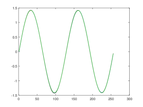
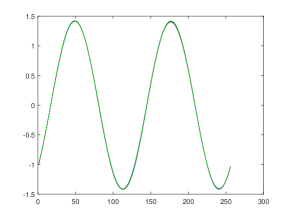
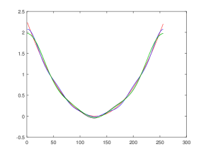
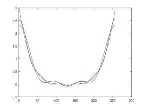
Figure 1: True functions (red) and their estimators: “Clustering before” (blue), “Clustering after” (green) and “No clustering” (black). Results for the functions in (4.3) and the kernel $g_{1}$ in (4.2) with $\lambda=3$ and SNR=3. Top row: $h_{1}$ (left), $h_{2}$ (right). Bottom row: $h_{3}$ (left), $h_{4}$ (right).

  

  

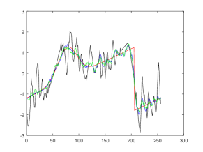
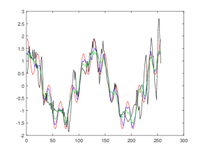
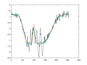
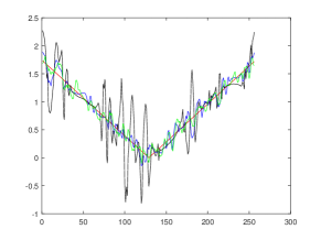
Figure 2: True functions (red) and their estimators: “Clustering before” (blue), “Clustering after” (green) and “No clustering” (black). Results for the functions in (4.4) and the kernel $g_{1}$ in (4.2) with $\lambda=3$ and SNR=3. Top row: $h_{1}$ (left), $h_{2}$ (right). Bottom row: $h_{3}$ (left), $h_{4}$ (right).

5 Conclusions

In this paper, we investigate theoretically and via a limited simulation study, the effect of clustering on the accuracy of recovery in ill-posed linear inverse problems. As we have stated earlier, in many applications leading to such problems, clustering is carried out at a pre-processing step and later is totally forgotten when it comes to error evaluation. Our main objective has been to evaluate what effect clustering at the pre-processing step has on the precision of the resulting estimators.

It appears that benefits of pre-clustering depend significantly on the nature of the inverse problem at hand. If the problem is moderately ill-posed (kernel $g_{1}$ in (4.2), $\alpha=\beta=0$), then, as Corollary 1 shows, the “Clustering Before” estimator has asymptotically smaller errors than the “No Clustering” estimator when the number of functions and the sample size grow. Tables 1 and 2, corresponding to this case, confirm that, for the finite number of functions and moderate sample size, the “Clustering before” procedure delivers better precision than the “Clustering after” and “No clustering” techniques. Furthermore, the “Clustering before” estimation has profound computational benefits since one needs to recover $K$ unknown functions instead of $M$. Moreover, the advantages of clustering at pre-processing step become more prominent when the problem is less ill-posed (larger $\lambda$). Indeed, in the case when the problem is not ill-posed ($\alpha=\beta=\gamma=0$ in (2.13)), as findings of Klopp et al. [17] show, clustering always improves estimation precision.

The situation changes drastically if the inverse problem is severely ill-posed (kernel $g_{2}$ in (4.2), $\alpha>0,\beta>0$). Our theoretical results indicate that clustering, in this case, does not improve the estimation precision as the number of functions and the sample size grow. These findings are consistent with the simulation study. In the case of functions in (4.4), Table 4 implies that the precisions of all three methodology are approximately the same, and the estimation errors are high even when clustering errors are small or zero. This is due to the fact that the reduction in the noise level due to clustering is not sufficient to counteract the ill-posedness of the problem and, thus, it does not lead to a meaningful improvement in estimation accuracy. Table 3, that reports on the simulations with functions in (4.3), presents an even more grim picture. Since functions in the set (4.3) resemble each other to start with and convolutions with the kernel $g_{2}$ make them to appear even more similar, “Clustering before” procedure leads to relatively high clustering errors that, in turn, produce higher estimation errors than the “Clustering after” and “No clustering” techniques.

In conclusion, clustering at the pre-processing step is beneficial when the problem is moderately ill-posed. It should be applied with extreme care when the problem is severely ill-posed.

6 Proofs

6.1 Proof of the oracle inequality

Proof of Theorem 1.  The proof of the inequality (3.2) is based on the standard techniques for proofs of oracle inequalities. We use optimization problem (2.18) to present the left-hand side as a sum of the error of any estimator plus the random error term followed by the difference between the penalty terms. Later on, we upper-bound the random error term for any number of classes $K$, any clustering matrix $Z$ and any set $J$. After that, we take a union bound over all possible $K$, $Z$ and $J$ to obtain an upper bound for the probability that the error exceeds certain threshold. The novelty of the proof lies in the fact that we are using vectorization of the model which allows us to attain the upper bounds.

Note that it follows from the optimization problem (2.18) that for any fixed $\mathbf{G},\mathbf{Z},J$ and $K$ one has

$$\|\widehat{\mathbf{G}}\|_{F}^{2}-2{\rm Tr}(\mathbf{Y}^{T}\mbox{$\Upsilon$}\widehat{\mathbf{G}}\mbox{$\Pi$}_{\hat{\mathbf{Z}},\hat{K}})+\mbox{Pen}(\hat{J},\hat{K})\leq\|\mathbf{G}\|_{F}^{2}-2{\rm Tr}(\mathbf{Y}^{T}\mbox{$\Upsilon$}\mathbf{G}\mbox{$\Pi$}_{\mathbf{Z},K})+\mbox{Pen}(J,K).$$

Then, adding and subtracting $\mathbf{G}_{*}$, we obtain

$$\|\widehat{\mathbf{G}}-\mathbf{G}_{*}\|_{F}^{2}+\|\mathbf{G}_{*}\|_{F}^{2}+2{\rm Tr}((\widehat{\mathbf{G}}-\mathbf{G}_{*})^{T}\mathbf{G}_{*})-2{\rm Tr}(\mathbf{Y}^{T}\mbox{$\Upsilon$}\widehat{\mathbf{G}}\mbox{$\Pi$}_{\hat{\mathbf{Z}},\hat{K}})+\mbox{Pen}(\hat{J},\hat{K})\leq$$

$$\|\mathbf{G}-\mathbf{G}_{*}\|_{F}^{2}+\|\mathbf{G}_{*}\|_{F}^{2}+2{\rm Tr}((\mathbf{G}-\mathbf{G}_{*})^{T}\mathbf{G}_{*})-2{\rm Tr}(\mathbf{Y}^{T}\mbox{$\Upsilon$}\mathbf{G}\mbox{$\Pi$}_{\mathbf{Z},K})+\mbox{Pen}(J,K).$$

Combine the trace product terms and recall that, due to equation (2.5), $\mathbf{Y}=\mbox{$\Upsilon$}^{-1}\mathbf{G}_{*}+\delta\mathbf{E}$. Hence, the last inequality yields

$$\|\widehat{\mathbf{G}}-\mathbf{G}_{*}\|_{F}^{2}\leq\|\mathbf{G}-\mathbf{G}_{*}\|_{F}^{2}+{2\,\delta}\,{\rm Tr}[\mathbf{E}^{T}\mbox{$\Upsilon$}(\widehat{\mathbf{G}}-\mathbf{G})]+\mbox{Pen}(J,K)-\mbox{Pen}(\hat{J},\hat{K})$$ (6.1)

We choose $\mathbf{G}=\mathbf{W}_{J}\mathbf{G}_{*}\mbox{$\Pi$}_{\mathbf{Z},K}$ and, in order to analyze the cross term ${\rm Tr}[\mathbf{E}^{T}\mbox{$\Upsilon$}(\widehat{\mathbf{G}}-\mathbf{G})]$, we use vectorization of the model. For this purpose, we choose $\mathbf{S}$ such that $\mbox{$\Sigma$}=\mathbf{S}\mathbf{S}^{T}$ and denote

$$\mbox{$\Pi$}_{\hat{\mathbf{Z}},\hat{K},\hat{J}}=(\mbox{$\Pi$}_{\hat{\mathbf{Z}},\hat{\mathbf{K}}}\otimes\mathbf{W}_{\hat{J}}),\quad\mbox{$\Pi$}_{\mathbf{Z},K,J}=(\mbox{$\Pi$}_{\mathbf{Z},K}\otimes\mathbf{W}_{J})$$ (6.2)

$$\hat{\mathbf{g}}=\mbox{vec}(\widehat{\mathbf{G}}),\quad\mathbf{g}=\mbox{vec}(\mathbf{G}),\quad\mbox{$\epsilon$}=\mbox{vec}(\mathbf{E}),\quad\mbox{$\Gamma$}=(\mathbf{I}_{M}\otimes\mbox{$\Upsilon$}),\quad\mbox{$\eta$}=(\mathbf{I}_{M}\otimes\mathbf{S}^{-1})\mbox{$\epsilon$}.$$ (6.3)

By definition of the matrix-variate normal distribution (Theorem 2.3.1 of Gupta and Nagar (2000)) and (2.8), we derive that

$$\mbox{$\epsilon$}\sim N(0,\mbox{$\Sigma$}\otimes\mathbf{I}_{M})$$ (6.4)

Then, ${\mathbb{E}}(\mbox{$\eta$}\mbox{$\eta$}^{T})=\mathbf{I}_{nM}$, so that, $\mbox{$\eta$}\sim N(0,\mathbf{I}_{nM})$, where $\epsilon$ is defined in (6.3) and $\|\mathbf{S}\|_{op}\leq C_{\psi}$. Then, equation (2.7) can be re-written as

$$\mbox{$\Gamma$}\mathbf{y}=\mathbf{g}_{*}+\delta\,\mbox{$\Gamma$}\,(\mathbf{I}_{M}\otimes\mathbf{S})\mbox{$\eta$}.$$ (6.5)

Observe that by Theorem 1.2.22 of Gupta and Nagar (2000), one has

$$\hat{\mathbf{g}}=\mbox{vec}(\mathbf{W}_{\hat{J}}\mbox{$\Upsilon$}\mathbf{Y}\mbox{$\Pi$}_{\hat{\mathbf{Z}},\hat{K}})=\mbox{$\Pi$}_{\hat{\mathbf{Z}},\hat{K},\hat{J}}\mbox{$\Gamma$}\mathbf{y},\quad\mathbf{g}=\mbox{$\Pi$}_{\mathbf{Z},K,J}\mathbf{g}_{*}$$

and ${\rm Tr}[\mathbf{E}^{T}\mbox{$\Upsilon$}(\widehat{\mathbf{G}}-\mathbf{G})]=\mbox{$\eta$}^{T}(\mathbf{I}_{M}\otimes\mathbf{S}^{T}\mbox{$\Upsilon$})(\mbox{$\Pi$}_{\hat{\mathbf{Z}},\hat{K},\hat{J}}\mbox{$\Gamma$}\mathbf{y}-\mbox{$\Pi$}_{\mathbf{Z},K,J}\mathbf{g}_{*})$. Now (6.1) can be rewritten in a vector form as

$$\|\hat{\mathbf{g}}-\mathbf{g}_{*}\|^{2}\leq\|\mathbf{g}-\mathbf{g}_{*}\|^{2}+\Delta+\mbox{Pen}(J,K)-\mbox{Pen}(\hat{J},\hat{K})$$ (6.6)

where

$$\Delta={2\,\delta}\mbox{$\eta$}^{T}(\mathbf{I}_{M}\otimes\mathbf{S}^{T}\mbox{$\Upsilon$})(\mbox{$\Pi$}_{\hat{\mathbf{Z}},\hat{K},\hat{J}}\mbox{$\Gamma$}\mathbf{y}-\mbox{$\Pi$}_{\mathbf{Z},K,J}\mathbf{g}_{*})=\Delta_{1}+\Delta_{2}$$ (6.7)

with

$$\Delta_{1}={2\,\delta}\mbox{$\eta$}^{T}(\mathbf{I}_{M}\otimes\mathbf{S}^{T}\mbox{$\Upsilon$})(\mbox{$\Pi$}_{\hat{\mathbf{Z}},\hat{K},\hat{J}}(\mbox{$\Gamma$}\mathbf{y}-\mathbf{g}_{*})),\quad\Delta_{2}={2\,\delta}\mbox{$\eta$}^{T}(\mathbf{I}_{M}\otimes\mathbf{S}^{T}\mbox{$\Upsilon$})(\mbox{$\Pi$}_{\hat{\mathbf{Z}},\hat{K},\hat{J}}-\mbox{$\Pi$}_{\mathbf{Z},K,J})\mathbf{g}_{*}.$$ (6.8)

Derivation of upper bounds for $\Delta_{1}$ and $\Delta_{2}$ is based on the following lemma.

Lemma 1.

Let $K,J$ be fixed, $\hat{J}$ be an arbitrary random subset of $\{1,\ldots,n\}$ and $\hat{K}$ be a random integer between 1 and $M$. Let $\mathbf{Z}\in{\mathcal{M}}(M,K)$ and $\widehat{\mathbf{Z}}\in{\mathcal{M}}(M,\hat{K})$ be a fixed and a random clustering matrix, respectively. Denote the projection matrices on the column spaces of matrices $\mathbf{Z}$ and $\widehat{\mathbf{Z}}$ by, respectively, $\mbox{$\Pi$}_{\mathbf{Z},K}$ and $\mbox{$\Pi$}_{\widehat{\mathbf{Z}},\hat{K}}$. Let $\mathbf{S}$ be a matrix with $\|\mathbf{S}\|_{op}\leq C_{\psi}$ and $\mbox{$\eta$}\sim N(0,\mathbf{I}_{nM})$. Then, for any $\tau>0$, there exist sets $\Omega_{1\tau}$ and $\Omega_{2\tau}$ with ${\mathbb{P}}(\Omega_{1\tau})\geq 1-\delta^{\tau}$ and ${\mathbb{P}}(\Omega_{2\tau})\geq 1-\delta^{\tau}$ such that

$$\|(\mbox{$\Pi$}_{\mathbf{Z},K}\otimes(\mathbf{W}_{J}\Upsilon\mathbf{S}))\mbox{$\eta$}\|^{2}\leq 2KC_{\psi}^{2}(\sum_{j\in J}\nu_{j}^{2})+3C_{\psi}^{2}(\max_{j\in J}\nu_{j}^{2})\tau\,\ln(\delta^{-1}),\quad\forall\omega\in\Omega_{1\tau};$$ (6.9)

$$\|(\mbox{$\Pi$}_{\widehat{\mathbf{Z}},\hat{K}} \otimes(\mathbf{W}_{\hat{J}}\Upsilon\mathbf{S}))\mbox{$\eta$}\|^{2}\leq 2\hat{K}C_{\psi}^{2}(\sum_{j\in\hat{J}}\nu_{j}^{2})$$ (6.10)

$$+3C_{\psi}^{2}(\max_{j\in\hat{J}}\nu_{j}^{2})\left\{M\ln\hat{K}+|\hat{J}|\ln(ne/|\hat{J}|)+\ln(Mn)+\tau\,\ln(\delta^{-1})\right\}\quad\forall\omega\in\Omega_{2\tau}.$$

Moreover, if $J=\left\{1,...,L\right\}$ is fixed and $\hat{J}=\left\{1,...,\hat{L}\right\}$ for some random integer $\hat{L}\geq 1$, then

$$\|(\mbox{$\Pi$}_{\mathbf{Z},K}\otimes(\mathbf{W}_{J}\Upsilon\mathbf{S}))\mbox{$\eta$}\|^{2}\leq 2KC_{\psi}^{2}\,\sum_{j=1}^{L}\nu_{j}^{2}+3C_{\psi}^{2}\,\tau\,\ln(\delta^{-1})\,\nu_{L}^{2},\quad\forall\omega\in\Omega_{1\tau};$$ (6.11)

$$\|(\mbox{$\Pi$}_{\widehat{\mathbf{Z}},\hat{K}} \otimes(\mathbf{W}_{\hat{J}}\Upsilon\mathbf{S}))\mbox{$\eta$}\|^{2}\leq 2\hat{K}C_{\psi}^{2}\,\sum_{j=1}^{L}\nu_{j}^{2}$$ (6.12)

$$+3C_{\psi}^{2}\,\nu_{L}^{2}\,\left\{M\ln\hat{K}+\ln(Mn)+\tau\,\ln(\delta^{-1})\right\}\quad\forall\omega\in\Omega_{2\tau}.$$

In what follows, we carry out only the proof of the upper bound (3.2) that takes place for a generic set $J$. The proof of the upper bound (3.3) can be obtained from the proof below with minimal modifications.

Note that $\Delta_{1}$ can be re-written as $\Delta_{1}=2\,\delta^{2}\,\mbox{$\eta$}^{T}(\mathbf{I}_{M}\otimes\mathbf{S}^{T}\mbox{$\Upsilon$})(\mbox{$\Pi$}_{\hat{\mathbf{Z}},\hat{K}}\otimes\mathbf{W}_{\hat{J}})(\mathbf{I}_{M}\otimes\mbox{$\Upsilon$}\mathbf{S})\mbox{$\eta$}$. Due to $\mbox{$\Gamma$}\mathbf{y}-\mathbf{g}_{*}=\delta\,\mbox{$\Gamma$}\mbox{$\epsilon$}$ and (6.3), we obtain $\Delta_{1}=2\,\delta^{2}\,\|(\mbox{$\Pi$}_{\hat{\mathbf{Z}},\hat{K}}\otimes(\mathbf{W}_{\hat{J}}\Upsilon\mathbf{S}))\mbox{$\eta$}\|^{2}$. Therefore, by (6.10), we obtain that for $\omega\in\Omega_{2\tau}$

$$|\Delta_{1}|\leq{2\,\delta^{2}\,C_{\psi}^{2}}\,\left[2\hat{K}\,\sum_{j\in\hat{J}}\nu_{j}^{2}+3(\max_{j\in\hat{J}}\nu_{j}^{2})\left\{M\ln\hat{K}+|\hat{J}|\ln(ne/|\hat{J}|)+\ln(Mn\delta^{-\tau})\right\}\right]$$ (6.13)

In order to construct an upper bound for $\Delta_{2}$, consider the following sets

$$\tilde{J}=J\cup\hat{J},\quad J_{1}=J\cap\hat{J},\quad J_{2}=J^{c}\cap\hat{J},\quad J_{3}=\hat{J}^{c}\cap J.$$ (6.14)

The sets $J_{1}$, $J_{2}$ and $J_{3}$ are non-overlapping and $\tilde{J}=J_{1}\cup J_{2}\cup J_{3}$. Furthermore, consider matrix $\tilde{\mathbf{Z}}$ that includes all linearly independent columns in matrices $\mathbf{Z}_{K}$ and $\hat{\mathbf{Z}}_{\hat{K}}$, so that $\mbox{Span}\{\tilde{\mathbf{Z}}\}=\mbox{Span}\{\mathbf{Z}_{K},\hat{\mathbf{Z}}_{\hat{K}}\}$. Let $\tilde{K}$ be the number of columns of matrix $\tilde{\mathbf{Z}}$. Then, one has

$$\mbox{$\Pi$}_{\hat{\mathbf{Z}},\hat{K}}\mbox{$\Pi$}_{\tilde{\mathbf{Z}},\tilde{K}}=\mbox{$\Pi$}_{\tilde{\mathbf{Z}},\tilde{K}}\mbox{$\Pi$}_{\hat{\mathbf{Z}},\hat{K}}=\mbox{$\Pi$}_{\hat{\mathbf{Z}},\hat{K}},$$

$$\mathbf{W}_{J}=\mathbf{W}_{J_{1}}+\mathbf{W}_{J_{3}},\ \mathbf{W}_{\hat{J}}=\mathbf{W}_{J_{1}}+\mathbf{W}_{J_{2}},\ \mathbf{W}_{\tilde{J}}=\mathbf{W}_{J_{1}}+\mathbf{W}_{J_{2}}+\mathbf{W}_{J_{3}}.$$

In order to obtain an upper bound for $\Delta_{2}$ defined in (6.8), note that using notations above, we can rewrite $\Delta_{2}$ as

$$\Delta_{2} ={2\,\delta}\mbox{$\eta$}^{T}(\mathbf{I}_{M}\otimes\mathbf{S}^{T}\mbox{$\Upsilon$})[(\mbox{$\Pi$}_{\hat{\mathbf{Z}},\hat{K}}\otimes\mathbf{W}_{J_{2}})+(\mbox{$\Pi$}_{\hat{\mathbf{Z}},\hat{K}}\otimes\mathbf{W}_{J_{1}})-(\mbox{$\Pi$}_{\mathbf{Z},K}\otimes\mathbf{W}_{J_{1}})-(\mbox{$\Pi$}_{\mathbf{Z},K}\otimes\mathbf{W}_{J_{3}})]\mathbf{g}_{*}$$

$$={2\,\delta}\mbox{$\eta$}^{T}(\mathbf{I}_{M}\otimes\mathbf{S}^{T}\mbox{$\Upsilon$})[(\mbox{$\Pi$}_{\hat{\mathbf{Z}},\hat{K}}\otimes\mathbf{W}_{J_{2}})+(\mbox{$\Pi$}_{\tilde{\mathbf{Z}},\tilde{K}}\otimes\mathbf{W}_{J_{1}})+(\mbox{$\Pi$}_{\mathbf{Z},K}\otimes\mathbf{W}_{J_{3}})][(\mbox{$\Pi$}_{\hat{\mathbf{Z}},\hat{K}}\otimes\mathbf{W}_{J_{2}})$$

$$+(\mbox{$\Pi$}_{\hat{\mathbf{Z}},\hat{K}}\otimes\mathbf{W}_{J_{1}})-(\mbox{$\Pi$}_{\mathbf{Z},K}\otimes\mathbf{W}_{J_{1}})-(\mbox{$\Pi$}_{\mathbf{Z},K}\otimes\mathbf{W}_{J_{3}})]\mathbf{g}_{*}$$

$$={2\,\delta}\mbox{$\eta$}^{T}(\mathbf{I}_{M}\otimes\mathbf{S}^{T}\mbox{$\Upsilon$})[(\mbox{$\Pi$}_{\hat{\mathbf{Z}},\hat{K}}\otimes\mathbf{W}_{J_{2}})+(\mbox{$\Pi$}_{\tilde{\mathbf{Z}},\tilde{K}}\otimes\mathbf{W}_{J_{1}})+(\mbox{$\Pi$}_{\mathbf{Z},K}\otimes\mathbf{W}_{J_{3}})][(\mbox{$\Pi$}_{\hat{\mathbf{Z}},\hat{K},\hat{J}}-\mbox{$\Pi$}_{\mathbf{Z},K,J})]\mathbf{g}_{*}$$

Using Cauchy inequality and $2ab\leq 4a^{2}+b^{2}/4$, we obtain

$$|\Delta_{2}|\leq|\Delta_{2,1}|+|\Delta_{2,2}|,\quad|\Delta_{2,2}|=0.25\,\|(\mbox{$\Pi$}_{\hat{\mathbf{Z}},\hat{K},\hat{J}}\mathbf{g}_{*}-\mbox{$\Pi$}_{\mathbf{Z},K,J}\mathbf{g}_{*})\|^{2}$$ (6.15)

$$|\Delta_{2,1}|=4\,\delta^{2}\,\|[(\mbox{$\Pi$}_{\hat{\mathbf{Z}},\hat{K}}\otimes\mathbf{W}_{J_{2}})+(\mbox{$\Pi$}_{\tilde{\mathbf{Z}},\tilde{K}}\otimes\mathbf{W}_{J_{1}})+(\mbox{$\Pi$}_{\mathbf{Z},K}\otimes\mathbf{W}_{J_{3}})](\mathbf{I}_{M}\otimes\mbox{$\Upsilon$}\mathbf{S})\mbox{$\eta$}\|^{2}$$

Applying Cauchy Inequality to the term $\Delta_{2,1}$ and using that $J_{2}\subseteq\hat{J}$ and $J_{3}\subseteq J$ we rewrite

$$|\Delta_{2,1}|\leq 12\delta^{2}\,\left[\|(\mbox{$\Pi$}_{\hat{\mathbf{Z}},\hat{K}}\otimes(\mathbf{W}_{\hat{J}}\mbox{$\Upsilon$}\mathbf{S}))\mbox{$\eta$}\|^{2}+\|(\mbox{$\Pi$}_{\tilde{\mathbf{Z}},\tilde{K}}\otimes(\mathbf{W}_{J_{1}}\mbox{$\Upsilon$}\mathbf{S}))\mbox{$\eta$}\|^{2}+\|(\mbox{$\Pi$}_{\mathbf{Z},K}\otimes(\mathbf{W}_{J}\mbox{$\Upsilon$}\mathbf{S}))\mbox{$\eta$}]\|^{2}\right]$$

The upper bounds for the first and the third term in the inequality above can be obtained directly from Lemma 1. For the second term, note that since $\tilde{K}\leq K+\hat{K}$ and $J_{1}\subseteq J$ and $J_{1}\subseteq\hat{J}$ for any $\omega\in\Omega_{1\tau}\cap\Omega_{2\tau}$ one has

$$\|(\mbox{$\Pi$}_{\tilde{\mathbf{Z}},\tilde{K}}\otimes(\mathbf{W}_{J_{1}}\mbox{$\Upsilon$}\mathbf{S}))\mbox{$\eta$}\|^{2} \leq C_{\psi}^{2}\,\left[2K\,\sum_{j\in J}\nu_{j}^{2}+2\hat{K}\,\sum_{j\in\hat{J}}\nu_{j}^{2}\right.$$ (6.16)

$$\left.+3\,(\max_{j\in\hat{J}}\nu_{j}^{2})\left\{M\ln\hat{K}+|\hat{J}|\ln\left(\frac{ne}{|\hat{J}|}\right)+\ln(Mn)+\tau\ln(\delta^{-1})\right\}\right]$$

due to

$$\tilde{K}\sum_{j\in J_{1}}\nu_{j}^{2}\leq K\,\sum_{j\in J}\nu_{j}^{2}+\hat{K}\,\sum_{j\in\hat{J}}\nu_{j}^{2}.$$

Combining (6.16) with equations (6.9) and (6.10), we obtain for any $\omega\in\Omega_{1\tau}\cap\Omega_{2\tau}$

$$|\Delta_{2,1}| \leq 12\delta^{2}\,C_{\psi}^{2}\,\left[4\hat{K}\,\sum_{j\in\hat{J}}\nu_{j}^{2}+4K\,\sum_{j\in J}\nu_{j}^{2}+3(\max_{j\in J}\nu_{j}^{2})(\tau\ln n)\right.$$ (6.17)

$$\left.+6\,(\max_{j\in\hat{J}}\nu_{j}^{2})\left\{M\ln\hat{K}+|\hat{J}|\ln\left(\frac{ne}{|\hat{J}|}\right)+\ln(Mn)+\tau\ln(\delta^{-1})\right\}\right]$$

Now consider $|\Delta_{2,2}|$ defined in (6.15). Rewrite $|\Delta_{2,2}|$ as $|\Delta_{2,2}|=0.25\|(\mbox{$\Pi$}_{\hat{\mathbf{Z}},\hat{K},\hat{J}}\mathbf{g}_{*}-\mathbf{g}_{*})-(\mbox{$\Pi$}_{\mathbf{Z},K,J}\mathbf{g}_{*}-\mathbf{g}_{*})\|^{2}$, so that

$$|\Delta_{2,2}|\leq 0.5\,\|(\mbox{$\Pi$}_{\hat{\mathbf{Z}},\hat{K},\hat{J}}\mathbf{g}_{*}-\mathbf{g}_{*})\|^{2}+0.5\|(\mbox{$\Pi$}_{\mathbf{Z},K,J}\mathbf{g}_{*}-\mathbf{g}_{*})\|^{2}.$$

Since $\hat{\mathbf{g}}=\mbox{$\Pi$}_{\hat{\mathbf{Z}},\hat{K},\hat{J}}\mbox{$\Gamma$}\mathbf{y}$ and

$$\|(\mbox{$\Pi$}_{\hat{\mathbf{Z}},\hat{K},\hat{J}}\mbox{$\Gamma$}\mathbf{y}-\mathbf{g}_{*})\|^{2} =\|(\mbox{$\Pi$}_{\hat{\mathbf{Z}},\hat{K},\hat{J}}(\mathbf{g}_{*}+\delta\,\mbox{$\Gamma$}\mbox{$\epsilon$})-\mathbf{g}_{*})\|^{2}$$

$$=\|(\mathbf{I}-\mbox{$\Pi$}_{\hat{\mathbf{Z}},\hat{K},\hat{J}})\mathbf{g}_{*}\|^{2}+\delta^{2}\,\|\mbox{$\Pi$}_{\hat{\mathbf{Z}},\hat{K},\hat{J}}\,\mbox{$\Gamma$}\mbox{$\epsilon$}\|^{2},$$

we derive

$$\|\hat{\mathbf{g}}-\mathbf{g}_{*}\|^{2}\geq\|\mbox{$\Pi$}_{\hat{\mathbf{Z}},\hat{K},\hat{J}}\mathbf{g}_{*}-\mathbf{g}_{*}\|^{2}$$ (6.18)

Taking into account that $\mathbf{g}=\mbox{$\Pi$}_{\mathbf{Z},K,J}\mathbf{g}_{*}$, so that $\|\mathbf{g}-\mathbf{g}_{*}\|^{2}=\|\mbox{$\Pi$}_{\mathbf{Z},K,J}\mathbf{g}_{*}-\mathbf{g}_{*}\|^{2}$, we obtain

$$|\Delta_{2,2}|\leq 0.5\|\hat{\mathbf{g}}-\mathbf{g}_{*}\|^{2}+0.5\|\mathbf{g}-\mathbf{g}_{*}\|^{2}.$$ (6.19)

By combining upper bounds of $\Delta_{1}$, $\Delta_{2,1}$ and $\Delta_{2,2}$, we derive from (6.13) and (6.17)– (6.19) that for any $\omega\in\Omega_{1\tau}\cap\Omega_{2\tau}$, an upper bound for $\Delta$ can be written as

$$|\Delta| \leq 0.5\|\hat{\mathbf{g}}-\mathbf{g}_{*}\|^{2}+0.5\|\mathbf{g}-\mathbf{g}_{*}\|^{2}+{2\,\delta^{2}\,C_{\psi}^{2}}\left\{26\hat{K}\,\sum_{j\in\hat{J}}\nu_{j}^{2}+24K\,\sum_{j\in J}\nu_{j}^{2}\right.$$

$$\left.+39\,(\max_{j\in\hat{J}}\nu_{j}^{2})\left[M\ln\hat{K}+|\hat{J}|\ln\left(\frac{ne}{|\hat{J}|}\right)+\ln(Mn)+\tau\ln(\delta^{-1})\right]+18(\max_{j\in J}\nu_{j}^{2})\tau\ln(\delta^{-1})\right\}$$ (6.20)

Since it follows from (6.3) that $\|\widehat{\mathbf{G}}-\mathbf{G}_{*}\|_{F}^{2}=\|\hat{\mathbf{g}}-\mathbf{g}_{*}\|^{2}$, we obtain from (6.6) that for any $\mathbf{G}=\Pi_{\mathbf{Z},K,J}\mathbf{G}_{*}$ on the set $\Omega_{1\tau}\cap\Omega_{2\tau}$ one has

$$\|\widehat{\mathbf{G}} -\mathbf{G}_{*}\|_{F}^{2}\leq 3\|\mathbf{G}-\mathbf{G}_{*}\|_{F}^{2}+{2\,\delta^{2}\,C_{\psi}^{2}}\left\{48K\,\sum_{j\in J}\nu_{j}^{2}+36(\max_{j\in J}\nu_{j}^{2})\tau\ln\delta^{-1}+52\hat{K}\,\sum_{j\in\hat{J}}\nu_{j}^{2}\right.$$ (6.21)

$$\left.+78(\max_{j\in\hat{J}}\nu_{j}^{2})\left[M\ln\hat{K}+|\hat{J}|\ln\left(\frac{ne}{|\hat{J}|}\right)+\ln(Mn)+\tau\ln\delta^{-1}\right]\right\}+2[\mbox{Pen}(J,K)-\mbox{Pen}(\hat{J},\hat{K})]$$

Choose $\mbox{Pen}(J,K)$ in the form (2.22) and note that all terms containing $\hat{J}$ and $\hat{K}$ in (6.21) cancel. Finally we obtained for any $\mathbf{G}=\mathbf{W}_{J}\mathbf{G}_{*}\mbox{$\Pi$}_{\mathbf{Z},K}$ that with probability at least $1-2\delta^{\tau}$

$$\|\widehat{\mathbf{G}}-\mathbf{G}_{*}\|_{F}^{2} \leq 3\|\mathbf{G}-\mathbf{G}_{*}\|_{F}^{2}+{2\,\delta^{2}\,C_{\psi}^{2}}\left\{48K\,\sum_{j\in J}\nu_{j}^{2}+36(\max_{j\in J}\nu_{j}^{2})\tau\ln n\right\}+2\,\mbox{Pen}(J,K)$$

which yields (3.2).

6.2 Proof of the upper bounds for the error

Proof of Theorem 2.  Since, when $j$ is growing, coefficients $\mbox{$\Theta$}_{jk}$ are decreasing while the values of $\nu_{j}$ are increasing according to (2.13), the optimal set $J$ is of the form $J=\left\{1,\cdots,L\right\}$, so that $|J|=L$. Then, we find $(\hat{\mathbf{Z}},\widehat{\mathbf{G}},\hat{L},\hat{K})$ as a solution of optimization problem (2.18) with the penalty given by expression (2.23).

Note that for the true number of classes $K_{*}$ with $N_{k},k=1,\ldots,K_{*}$ elements in each class, $\mathbf{G}$ are coefficients of each $f_{m}$ and $\Theta$ is the clustered version of those coefficients. It follows from (2.4) that

$$R(\hat{\mathbf{f}},{\mathcal{S}}(r,{\mathcal{A}}),M,K_{*})\leq M^{-1}\|\widehat{\mathbf{G}}-\mathbf{G}_{*}\|_{F}^{2}+M^{-1}\sum_{k=1}^{K_{*}}\ N_{k}\sum_{j=n+1}^{\infty}\,\mbox{$\Theta$}_{jk}^{2}.$$ (6.22)

Therefore, application of the upper bound (3.3) with a generic $L$, $\mathbf{Z}=\mathbf{Z}_{*}$, $\mathbf{K}=K_{*}$, where $\mathbf{Z}_{*}$ and $K_{*}$ are respectively the true clustering matrix and the true number of classes, yields

$$M^{-1}\,\|\widehat{\mathbf{G}}-\mathbf{G}_{*}\|_{F}^{2}\leq 3\,M^{-1}\,\|\mathbf{W}_{J}\mathbf{G}_{*}\mbox{$\Pi$}_{\mathbf{Z}_{*},K_{*}}-\mathbf{G}_{*}\|_{F}^{2}+4\,M^{-1}\,\overline{\rm Pen}(L,K_{*})$$ (6.23)

where $\overline{\rm Pen}(L,K)$ is defined in (2.23). Observe that

$$\|\mathbf{W}_{J}\mathbf{G}_{*}\mbox{$\Pi$}_{\mathbf{Z}_{*},K_{*}}-\mathbf{G}_{*}\|_{F}^{2}=\|(\mathbf{W}_{J}-\mathbf{I}_{n})\mathbf{G}_{*}\|_{F}^{2}=\sum_{k=1}^{K^{*}}N_{k}\sum_{j=L+1}^{n}\mbox{$\Theta$}_{jk}^{2}$$ (6.24)

where $N_{k}$ is the number of functions $f_{m}=h_{k}$ in the cluster $k$, $k=1,\cdots,K^{*}$, and $\mbox{$\Theta$}_{jk}$ are the true coefficients of those functions. Hence, it follows from (2.11) that

$$\sum_{j=L+1}^{n}\mbox{$\Theta$}_{jk}^{2}\leq{\mathcal{A}}^{2}L^{-2r}.$$ (6.25)

Since $\displaystyle\sum_{k=1}^{K^{*}}N_{k}=M$, (6.24) and (6.25) yield

$$\|\mathbf{W}_{J}\mathbf{G}_{*}\mbox{$\Pi$}_{\mathbf{Z}_{*},K_{*}}-\mathbf{G}_{*}\|_{F}^{2}\leq{\mathcal{A}}^{2}ML^{-2r}$$ (6.26)

Moreover, it follows from (2.12) that

$$M^{-1}\ \sum_{k=1}^{K_{*}}\ N_{k}\sum_{j=n+1}^{\infty}\,\mbox{$\Theta$}_{jk}^{2}\leq{\mathcal{A}}^{2}n^{-2r}\asymp\delta^{2},$$

so that the last term in (6.22) is smaller than $C\,R(M,K_{*},\delta)$.

Now, consider the second term in (6.23). Due to the condition (2.13), one obtains

$$\nu_{L}^{2}\leq\aleph_{2}^{2}\,L^{2\gamma}\exp\left(2\alpha L^{\beta}\right),\quad\sum_{j=1}^{L}\nu_{j}^{2}\leq\aleph_{2}^{2}\,L^{2\gamma+1}\exp\left(2\alpha L^{\beta}\right).$$

Denote

$$R_{1}\equiv R_{1}(K_{*},\delta)\asymp K_{*},\quad R_{2}\equiv R_{2}(M,K_{*},\delta)\asymp M\ln K_{*}+\ln(\delta^{-1}).$$ (6.27)

Therefore, it follows from (2.22) and (3.2) that, under condition (3.5),

$$\frac{\|\widehat{\mathbf{G}}-\mathbf{G}_{*}\|_{F}^{2}}{M}\leq\tilde{C}\,\min_{L}\left\{L^{-2r}+\frac{\delta^{2}\,L^{2\gamma}\,\exp(2\alpha L^{\beta})}{M}\,\left[LR_{1}(K_{*},\delta)+R_{2}(M,K_{*},\delta)\right]\right\}\ \ \ \$$ (6.28)

where $R_{1}(K_{*},\delta)$ and $R_{2}(M,K_{*},\delta)$ are defined in (6.27) and $\tilde{C}$ depends only on $\mu$, ${\mathcal{A}}$, $\aleph_{2}$, $C_{\psi}^{2}$ and is independent of $M$, $L$, $\delta$ and $K_{*}$.

In order to find the minimum of the right hand side of (6.28), denote

$$R(L,M,K_{*},\delta)=L^{-2r}+\delta^{2}\,M^{-1}\,\exp\left(2\alpha L^{\beta}\right)\left[L^{2\gamma+1}R_{1}+L^{2\gamma}R_{2}\right]$$ (6.29)

and observe that

$$M^{-1}\,\|\widehat{\mathbf{G}}-\mathbf{G}_{*}\|_{F}^{2}\leq\tilde{C}\,\min_{L}R(L,M,K_{*},\delta)$$ (6.30)

where $L_{opt}$ is the value of $L$ minimizing the right hand side of (6.28). Denote

$$L_{1,opt}=\underset{L}{\operatorname{argmin}}\,[L^{-2r}+\delta^{2}\,M^{-1}\,\exp\left(2\alpha L^{\beta}\right)L^{2\gamma+1}R_{1}],$$ (6.31)

$$L_{2,opt}=\underset{L}{\operatorname{argmin}}\,[L^{-2r}+\delta^{2}\,M^{-1}\,\exp\left(2\alpha L^{\beta}\right)L^{2\gamma}R_{2}].$$ (6.32)

It is easy to see that since the first terms in expressions (6.31) and (6.32) are decreasing in $L$ while the second terms are increasing, the values $L_{1,opt}$ and $L_{2,opt}$ are such that those terms are equal to each other up to a multiplicative constant. Then, $R(L_{opt},M,K_{*},\delta)=\max\left\{L_{1,opt}^{-2r},L_{2,opt}^{-2r}\right\}$, and, due to $\max(a,b)\asymp a+b$ for positive $a$ and $b$, we obtain

$$R(L_{opt},M,K_{*},\delta)\asymp L_{1,opt}^{-2r}+L_{2,opt}^{-2r}.$$ (6.33)

Consider two cases.

Case 1: $\alpha=\beta=0$.  Direct calculations yield

$$L_{1,opt}\asymp\left(M^{-1}\delta^{2}R_{1}\right)^{-\frac{1}{2\gamma+2r+1}},\quad L_{2,opt}\asymp\left(M^{-1}\delta^{2}R_{2}\right)^{-\frac{1}{2\gamma+2r}},$$

so that, due to (6.27),

$$L_{1,opt}=(M^{-1}\,\delta^{2}K_{*})^{-\frac{1}{2\gamma+2r+1}},\quad L_{2,opt}=[\delta^{2}(\ln K_{*}+M^{-1}\ln\delta^{-1})]^{-\frac{1}{2\gamma+2r}}$$

Then, by (6.33),

$$R(L_{opt},M,K_{*},\delta)\asymp(M^{-1}\,\delta^{2}K_{*})^{\frac{2r}{2\gamma+2r+1}}+[\delta^{2}(\ln K_{*}+M^{-1}\ln\delta^{-1})]^{\frac{2r}{2\gamma+2r}}.$$ (6.34)

Now, in order to obtain the expression (3.6), note that if $K_{*}\geq 2$, then $\ln K_{*}$ dominates $M^{-1}\ln\delta^{-1}$. If $K_{*}=1$, then (6.34) can be re-written as

$$R(L_{opt},M,K_{*},\delta)\asymp\left(\frac{\delta^{2}}{M}\right)^{\frac{2r}{2\gamma+2r+1}}\left[1+\left(\frac{\delta^{2}}{M}\right)^{\frac{2r}{(2\gamma+2r+1)(2r+2\gamma)}}(\ln\delta^{-1})^{\frac{2r}{2\gamma+2r}}\right]\asymp\left(\frac{\delta^{2}K_{*}}{M}\right)^{\frac{2r}{2\gamma+2r+1}},$$

which yields (3.6).

Case 2: $\alpha>0,\beta>0$.  Minimizing expressions in (6.31) and (6.32), we obtain

$$L_{i,opt}\asymp\left\{\left[\ln\left(\frac{M}{\delta^{2}R_{i}}\right)\right]\right\}^{\frac{1}{\beta}},\quad i=1,2,$$

If $K_{*}\geq 2$, then $R_{2}\geq R_{1}$. Taking into account that, under assumption (3.5), for large $M$ and small $\delta$, $\ln\left(M\delta^{-2}\ln M\right)\asymp\ln\left(M\delta^{-2}\right)$ and $\ln(Mn)\asymp\ln M$, we obtain

$$L_{1,opt}=\min\left\{\left[\ln\left(\frac{M}{\delta^{2}K_{*}}\right)\right];\left[\ln\left(\frac{M}{\delta^{2}\ln M}\right)\right]\right\}^{\frac{1}{\beta}}\asymp\left[\ln\left(\frac{M}{\delta^{2}K_{*}}\right)\right]^{\frac{1}{\beta}}.$$

Similarly,

$$L_{2,opt}=\min\left\{\left[\ln\left(\frac{1}{\delta^{2}\ln K_{*}}\right)\right];\left[\ln\left(\frac{M}{\delta^{2}\ln M}\right)\right]\right\}^{\frac{1}{\beta}}\asymp\left[\ln\left(\frac{1}{\delta^{2}\ln K_{*}}\right)\right]^{\frac{1}{\beta}},$$

which, together with (6.30) and (6.33), yield the expression (3.7). One can easily check that the case of $K_{*}=1$ leads to the same results.

6.3 Proofs of the minimax lower bounds for the error

Proof of Theorem 3.  Since the estimation error is comprised of the error due to nonparametric estimation and to clustering, we consider two cases here.

Lower bound for the error due to clustering.
Let $K\geq 2$ be the fixed number of classes. Consider a subset ${\cal{Z}}(M,K)\subset{\mathcal{M}}(M,K)$ of the set of all clustering matrices which contains all matrices that cluster $\frac{M}{K}$ vectors into each class. By Lemma 5 in Pensky (2019) with $\gamma=1$, obtain that the cardinality of the set ${\cal{Z}}(M,K)$ is

$$|{\cal{Z}}(M,K)|=M!\Big{/}[(M/K)!]^{K}\geq\exp\left(M\ln K/4\right)$$ (6.35)

Let set $J$ be of the form $J=\{L_{1},...,L_{2}\}$ where $1\leq L_{1}<L_{2}\leq n$ and $n=[\delta^{-2}]$. Choose $\mbox{$\Theta$}_{jk}=0$ if $j\notin J$. In what follows, we use the Packing Lemma (Lemma 4 of Pensky (2019)):

Lemma 2.

(The Packing lemma). Let ${\cal{Z}}(M,K)\subseteq{\mathcal{M}}(M,K)$ be a collection of clustering matrices and $q$ be a positive constant. Then, there exists a subset ${\mathcal{S}}_{M,K}(q)\subset{\cal{Z}}(M,K)$ such that for $\mathbf{Z}_{1},\mathbf{Z}_{2}\in{\mathcal{S}}_{M,K}(q)$ one has $\|\mathbf{Z}_{1}-\mathbf{Z}_{2}\|_{H}=\|\mathbf{Z}_{1}-\mathbf{Z}_{2}\|^{2}_{F}\geq q$ and $\ln|{\mathcal{S}}_{M,K}(q)|\geq\ln|{\cal{Z}}(M,K)|-q\ln(MKe/q)$.

Apply this lemma with $q=dM$, $0<d<1/4$. Then, by (6.35), derive

$$\ln|{\mathcal{S}}_{M,K}\left(dM\right)|\geq M\,\left[\ln K-4d\ln(Ke/d)\right]\big{/}4.$$

Use the following statement:

Lemma 3.

If $K\geq 2$ and $d$ is such that

$$d-d\ln d\leq(\ln 2)/9,\quad d\leq 1/9,$$ (6.36)

then $\ln K-4d\ln(Ke/d)\geq(\ln K)/9$.

It is easy to calculate that, e.g., $d=0.0147$ satisfies the condition (6.36). Then, for $d$ obeying (6.36), one has

$$\ln|{\mathcal{S}}_{M,K}(dM)|\geq\frac{M}{36}\ln K,\quad\|\mathbf{Z}_{1}-\mathbf{Z}_{2}\|_{H}\geq dM\ \mbox{for any}\ \mathbf{Z}_{1},\mathbf{Z}_{2}\in{\mathcal{S}}_{M,K}(dM),\ \mathbf{Z}_{1}\neq\mathbf{Z}_{2}$$ (6.37)

Consider a collection of binary vectors ${\mbox{$\omega$}}\in\{0,1\}^{|J|}$. By Varshamov-Gilbert bound lemma, there exists a subset ${\cal W}$ of those vectors such that, for any ${\mbox{$\omega$}},{\mbox{$\omega$}^{\prime}}\in{\cal W}$ such that ${\mbox{$\omega$}}\neq{\mbox{$\omega$}^{\prime}}$ one has $\|{\mbox{$\omega$}}-{\mbox{$\omega$}^{\prime}}\|_{H}\geq|J|/8$ and $\ln{|{\cal W}|}\geq|J|\ln(2)/8$. Choose a subset ${\cal W}_{K}$ of ${\cal W}$ such that $|{\cal W}_{K}|=K$. This is possible if $K\leq 2^{|J|/8}$ which is equivalent to $|J|\geq 8\,\ln K/\ln 2$. Consider a set of vectors $\mathbf{w}\in\{0,1\}^{n}$ obtained by packing $\omega$ with zeros for components not in $J$. Then

$${\cal W}_{K}=\left\{{\mathbf{w}_{1}},...,{\mathbf{w}_{K}}\in\{0,1\}^{n}:\,\|\mathbf{w}_{i}\|_{0}\leq|J|,\ \|\mathbf{w}_{i}-\mathbf{w}_{j}\|_{0}\geq|J|/8,\ i\neq j\right\}$$ (6.38)

Define matrix $\mathbf{W}$ with columns $\mathbf{w}_{k}$, $k=1,...,K$. Finally, form the set ${\mathcal{G}}_{M,K}$ of matrices $\mathbf{G}$ of the form

$${\mathcal{G}}_{M,K}=\left\{\mathbf{G}\in R^{n\times M}:\mathbf{G}=\theta\mathbf{W}\mathbf{Z}^{T},\mathbf{Z}\in{\mathcal{S}}_{M,K}(dM)\right\}$$

where $d$ satisfies (6.36) and $\theta>0$ depends on $M$,$\delta$ and $K$. Note that, due to (6.37), one has

$$\ln|{\mathcal{G}}_{M,K}|\geq(M\ln K)/36$$ (6.39)

Let $\mathbf{Z}_{1},\mathbf{Z}_{2}\in{\mathcal{S}}_{M,K}$ be two clustering matrices. Set $\mathbf{G}_{1}=\theta\mathbf{W}\mathbf{Z}_{1}^{T}$ $\mathbf{G}_{2}=\theta\mathbf{W}\mathbf{Z}_{2}^{T}$, so that $\mathbf{G}_{1},\mathbf{G}_{2}\in{\mathcal{G}}_{M,K}$. Since for any $i,i^{\prime}$ one has $\|{\mathbf{w}}_{i}-{\mathbf{w}}_{i^{\prime}}\|_{0}=\|{\mathbf{w}}_{i}-{\mathbf{w}}_{i^{\prime}}\|^{2}$, derive that

$$\|\theta\mathbf{W}\left(\mathbf{Z}_{1}-\mathbf{Z}_{2}\right)^{T}\|_{F}^{2}=\sum_{m=1}^{M}\sum_{j=1}^{n}\theta^{2}\left[\left(\mathbf{w}_{z_{1}{\left(m\right)}}\right)_{j}-\left(\mathbf{w}_{z_{2}{\left(m\right)}}\right)_{j}\right]^{2}=$$

$$=\theta^{2}\sum_{m=1}^{M}\|{\mathbf{w}}_{z_{1}\left(m\right)}-{\mathbf{w}}_{z_{2}\left(m\right)}\|^{2}\geq\#\{m:z_{1}\left(m\right)\neq z_{2}\left(m\right)\}\,\theta^{2}|J|/8.$$ (6.40)

On the other hand, observe that for $\mathbf{Z}_{1},\mathbf{Z}_{2}\in{\mathcal{S}}_{M,K}$ one has

$$\#\{m:z_{1}\left(m\right)\neq z_{2}\left(m\right)\}=0.5\,\|\mathbf{Z}_{1}-\mathbf{Z}_{2}\|_{H}\geq dM/2.$$

Therefore, the last two inequalities yield for any $\mathbf{G}_{1},\mathbf{G}_{2}\in{\mathcal{G}}_{M,K}$

$$\|\mathbf{G}_{1}-\mathbf{G}_{2}\|_{F}^{2}\geq d\,\theta^{2}|J|M/16.$$ (6.41)

Now, it is easy to calculate that for any $\mathbf{G}_{1},\mathbf{G}_{2}\in{\mathcal{G}}_{M,K}$ and the corresponding probability measures $P_{\mathbf{G}_{1}}$ and $P_{\mathbf{G}_{2}}$ associated with $\mathbf{Y}=\mbox{$\Upsilon$}^{-1}\mathbf{G}_{i}+\delta\mathbf{E}$, $i=1,2$, in (2.5), one has the following inequality for the Kullback-Leibler divergence between $P_{\mathbf{G}_{1}}$ and $P_{\mathbf{G}_{2}}$:

$$K\left(P_{\mathbf{G}_{1}},P_{\mathbf{G}_{2}}\right)\leq\frac{1}{2\delta^{2}C_{\psi}^{2}}\|\mbox{$\Upsilon$}^{-1}\left(\mathbf{G}_{2}-\mathbf{G}_{1}\right)\|_{F}^{2}$$ (6.42)

Since $\mathbf{G}_{1}=\theta\mathbf{W}\mathbf{Z}_{1}$, $\mathbf{G}_{2}=\theta\mathbf{W}\mathbf{Z}_{2}$, we obtain

$$\|\mbox{$\Upsilon$}^{-1}\left(\mathbf{G}_{2}-\mathbf{G}_{1}\right)\|_{F}^{2}\leq\theta^{2}\,\|\mathbf{Z}_{2}-\mathbf{Z}_{1}\|_{op}^{2}\,\|\mbox{$\Upsilon$}^{-1}\mathbf{W}\|_{F}^{2}$$ (6.43)

Note that ${\mathcal{S}}_{M,K}(dM)\subset{\cal{Z}}(M,K)$, so that for any $\mathbf{Z}\in{\mathcal{S}}_{M,K}(dM)$ one has $\mathbf{Z}^{T}\mathbf{Z}=(M/K)\,\mathbf{I}_{K}$, hence $\|\mathbf{Z}\|_{op}=\sqrt{M/K}$. Then, $\|\mathbf{Z}_{1}-\mathbf{Z}_{2}\|_{op}^{2}\leq 4M/K$. Also, due to $J=\{L_{1},...,L_{2}\}$ and condition (2.13), one has

$$\sum_{j\in J}\nu_{j}^{-2}\leq\aleph_{1}^{-2}|J|\,L_{1}^{-2\gamma}\exp\left(-2\alpha L_{1}^{\beta}\right).$$ (6.44)

Since $\|\mbox{$\Upsilon$}^{-1}\mathbf{W}\|_{F}^{2}\leq\sum_{k=1}^{K}\sum_{j\in J}\nu_{j}^{-2}$, obtain

$$K\left(P_{\mathbf{G}_{1}},P_{\mathbf{G}_{2}}\right)\leq\frac{2}{\delta^{2}\aleph_{1}^{2}C_{\psi}^{2}}\ \theta^{2}|J|M\,L_{1}^{-2\gamma}\exp\left(-2\alpha L_{1}^{\beta}\right).$$ (6.45)

Finally, due to condition (2.11), one needs $\theta^{2}\sum_{j\in J}(j+1)^{2r}\leq{\mathcal{A}}^{2}$, so that we can choose

$$\theta^{2}={\mathcal{A}}^{2}|J|^{-1}L_{2}^{-2r}$$ (6.46)

In order to apply Theorem 2.5 of Tsybakov (2009) with $\alpha=1/9$, we need $K\left(P_{\mathbf{G}_{1}},P_{\mathbf{G}_{2}}\right)\leq\ln|{\mathcal{G}}_{M,K}|/9$ which, due to (6.37), is guaranteed by

$$\frac{\theta^{2}|J|}{\delta^{2}\aleph_{1}^{2}C_{\psi}^{2}}L_{1}^{-2\gamma}\exp\left(-2\alpha L_{1}^{\beta}\right)\leq\frac{\ln K}{648}.$$ (6.47)

If inequality (6.47) holds, then application of Theorem 2.5 of Tsybakov (2009) yields that, with probability at least 0.1, one has (3.9) where, due to (3.1) and (6.41),

$$R_{\min}(M,K_{*},\delta)=\theta^{2}|J|.$$ (6.48)

Consider $L_{1}=L/2+1$ and $L_{2}=L$, so that

$$\theta^{2}\asymp L^{-(2r+1)},\quad R_{\min}(M,K_{*},\delta)\asymp L^{-2r}.$$ (6.49)

If $\alpha=0$ , $\beta=0$, then, by (6.49), inequality (6.47) holds if $L\asymp\left(\delta^{2}\,\ln K\right)^{-\frac{1}{2r+2\gamma}}.$ Hence,

$$R_{\min}(M,K_{*},\delta)\gtrsim\left(\delta^{2}\,\ln K_{*}\right)^{\frac{2r}{2r+2\gamma}}.$$ (6.50)

If $\alpha>0$, $\beta>0$, then inequality (6.47) holds if $L^{-(2\gamma+2r)}\exp\left(-2\alpha L^{\beta}\right)\lesssim\delta^{2}\ln K$, so that $L\asymp\left[\ln\left(\frac{1}{\delta^{2}\ln K}\right)\right]^{\frac{1}{\beta}}$. Therefore,

$$R_{\min}(M,K_{*},n)\gtrsim\left[\ln\left(\frac{1}{\delta^{2}\ln K_{*}}\right)\right]^{-\frac{2r}{\beta}}.$$ (6.51)

Lower bound for the error due to estimation.
Let, as before, $n=[\delta^{-2}]$ and $J=\{L_{1},...,L_{2}\}$ where $1\leq L_{1}<L_{2}\leq n$. Consider a set of binary vectors $\mbox{$\omega$}\in\{0,1\}^{|J|K}$ and set $N=|J|K$. Complete vectors $\omega$ with zeros to obtain vectors $\mathbf{w}\in\{0,1\}^{nK}$. By Varshamov-Gilbert lemma, there exists a subset ${\mathcal{B}}$ of those vectors such that for any $\mathbf{w},\mathbf{w}^{\prime}\in{\mathcal{B}}$ such that $\mathbf{w}\neq\mathbf{w}^{\prime}$ one has $\|\mathbf{w}-\mathbf{w}^{\prime}\|_{H}\geq N/8$ and $\ln|{\mathcal{B}}|\geq N\ln(2)/8$. Pack vectors $\mathbf{w}$ into matrices $\mathbf{W}\in\{0,1\}^{n\times K}$. Denote the set of those matrices by ${\cal W}$ and observe that

$$\|\mathbf{W}_{1}-\mathbf{W}_{2}\|_{F}^{2}\geq N/8\quad\mbox{for all}\quad\mathbf{W}_{1},\mathbf{W}_{2}\in{\cal W},\ \mathbf{W}_{1}\neq\mathbf{W}_{2};\qquad\ln|{\cal W}|\geq(N\,\ln 2)/8.$$ (6.52)

Let $\mathbf{Z}$ be the clustering matrix that corresponds to uniform sequential clustering, $M/K$ vectors per class. Finally, form the set ${\mathcal{G}}_{M,K}$ of matrices $\mathbf{G}$ of the form

$${\mathcal{G}}_{M,K}=\left\{\mathbf{G}\in R^{M\times K}:\mathbf{G}=\theta\mathbf{W}\mathbf{Z}^{T},\quad\mathbf{W}\in{\cal W}\right\}$$

where $\theta>0$ depends on $M$,$\delta$ and $K$. Then, for any $\mathbf{G}_{1},\mathbf{G}_{2}\in{\mathcal{G}}_{M,K}$, $\mathbf{G}_{1}\neq\mathbf{G}_{2}$, due to $\mathbf{Z}^{T}\mathbf{Z}=(M/K)\,\mathbf{I}_{K}$ and (6.52), obtain

$$\|(\mathbf{G}_{1}-\mathbf{G}_{2})\|^{2}_{F}=\theta^{2}\|(\mathbf{W}_{1}-\mathbf{W}_{2})\mathbf{Z}^{T}\|_{F}^{2}=\frac{\theta^{2}M}{K}\,\|\mathbf{W}_{1}-\mathbf{W}_{2}\|^{2}_{F}\geq\frac{\theta^{2}MN}{8K}$$ (6.53)

Now, since $\mathbf{G}_{1}=\theta\mathbf{W}_{1}\mathbf{Z}$ and $\mathbf{G}_{2}=\theta\mathbf{W}_{2}\mathbf{Z}$, using formula (6.42), derive that

$$K\left(P_{\mathbf{G}_{1}},P_{\mathbf{G}_{2}}\right)\leq\frac{\theta^{2}}{2\delta^{2}C_{\psi}^{2}}\|\mbox{$\Upsilon$}^{-1}\left(\mathbf{W}_{2}-\mathbf{W}_{1}\right)\|_{F}^{2}\,\|\mathbf{Z}\|_{op}^{2}$$

Recalling that $\|\mathbf{Z}\|_{op}^{2}=M/K$ and $\|\mbox{$\Upsilon$}^{-1}\left(\mathbf{W}_{2}-\mathbf{W}_{1}\right)\|_{F}^{2}\leq\sum_{k=1}^{K}\sum_{j\in J}\nu_{j}^{-2}$, and using (6.44), arrive at

$$K\left(P_{\mathbf{G}_{1}},P_{\mathbf{G}_{2}}\right)\leq\frac{M\theta^{2}}{2\delta^{2}\,\aleph_{1}^{2}\,C_{\psi}^{2}}\,|J|\,L_{1}^{-2\gamma}\exp\left(-2\alpha L_{1}^{\beta}\right).$$

In order to apply Theorem 2.5 of Tsybakov (2009)with $\alpha=1/9$, we need $K\left(P_{\mathbf{G}_{1}},P_{\mathbf{G}_{2}}\right)\leq(1/9)\ln|{\mathcal{G}}_{M,K}|$ which, due to (6.52), is guaranteed by

$$\frac{\theta^{2}M}{\delta^{2}\aleph_{1}^{2}C_{\psi}^{2}}L_{1}^{-2\gamma}\exp\left(-2\alpha L_{1}^{\beta}\right)\leq\frac{K}{36}.$$ (6.54)

If inequality (6.54) holds, then application of Theorem 2.5 of Tsybakov (2009) yields that, with probability at least 0.1, one has (3.9), where, due to (3.1) and (6.53),

$$R_{\min}(M,K_{*},\delta)\gtrsim\theta^{2}|J|$$ (6.55)

Now, as before, we consider two choices of $L_{1}$ and $L_{2}$: $L_{1}=L_{2}=L$ and $L_{1}=L/2+1$ , $L_{2}=L$ leading to the values of $\theta^{2}$ given by (6.49). Again, we consider the cases of $\alpha=\beta=0$ and $\alpha>0$, $\beta>0$ separately.

Case 1: $\alpha=0$ , $\beta=0$, $L_{1}=L/2+1$ , $L_{2}=L$, $|J|=L/2$.
Since $L_{1}\asymp L_{2}\asymp|J|\asymp L$, inequality (6.54) holds if $L\asymp\left(\delta^{2}M^{-1}\,K\right)^{-\frac{1}{2r+2\gamma+1}}$ and

$$R_{\min}(M,K_{*},\delta)\gtrsim\left(\delta^{2}\,M^{-1}\,K\right)^{\frac{2r}{2r+2\gamma+1}}.$$ (6.56)

Case 2: $\alpha>0$, $\beta>0$, $L_{1}=L_{2}=L$, $|J|=1$.
Plugging the first expression from (6.49) into (6.54), derive that $L^{-(2\gamma+2r)}\exp\left(-2\alpha L^{\beta}\right)\lesssim\delta^{2}M^{-1}K$, so that $L\asymp\left[\ln\left(\frac{M}{\delta^{2}K}\right)\right]^{\frac{1}{\beta}}$. Therefore,

$$R_{\min}(M,K_{*},\delta)\gtrsim\left[\ln\left(\frac{M}{\delta^{2}K}\right)\right]^{-\frac{2r}{\beta}}$$ (6.57)

Now, in order to obtain the expressions for the lower bounds, we find the maximum of (6.50) and (6.56) if $\alpha=0$ , $\beta=0$, and of (6.51) and (6.57) if $\alpha>0$ , $\beta>0$.

6.4 Proofs of the comparison of the risks with and without clustering

Proof of Corollary 1.  First observe that expressions (3.12) are obtained directly from (3.6) and (3.7) by setting $M=K_{*}=1$ since all functions belong to the same Sobolev ball (2.10). In order to compare the upper bounds (3.6) and (3.7) obtained with clustering with the upper bound (3.12) derived without clustering, we consider several cases.

Case 1 $\alpha=0$ , $\beta=0$.
Expressions in (3.13) are obtain by direct evaluation. Note that the second expression in the case of $K_{*}\geq 2$ tends to zero as $M\to\infty$ since, due to (3.5), $\ln K_{*}\leq\ln M\asymp\ln\delta^{-1}$.

Case 2 $\alpha>0$ , $\beta>0$.
Note that, due to the condition (3.5),

$$\ln(\delta^{-2})\leq\ln(M\delta^{-2}K_{*}^{-1})\leq\ln M+\ln(\delta^{-2})\asymp\ln(\delta^{-2}),$$

Also, for $K_{*}\geq 2$ and $\delta^{-2}\geq e$, due to $\ln x\leq x/2$ for $x\geq 1$, obtain

$$\ln\left(\delta^{-2}\,\ln(K_{*}^{-1})\right)=\ln(\delta^{-2})-\ln\ln K_{*}\geq\ln(\delta^{-2})-0.5\,\ln(\delta^{-2})\asymp\ln(\delta^{-2}),$$

which completes the proof.

6.5 Proofs of supplementary statements

Proof of Lemma 1.  Proof of Lemma 1 is based on the following statement provided in Gendre(2014)

Lemma 4.

(Gendre (2014)). Let $\mathbf{A}\in R^{p\times p}$ be a fixed matrix and $\mbox{$\epsilon$}\sim N(0,\mathbf{I}_{p})$. Then, for any $x>0$ one has

$${\mathbb{P}}\left\{\|\mathbf{A}\mbox{$\epsilon$}\|^{2}\geq{\rm Tr}(\mathbf{A}^{T}\mathbf{A})+2\,\sqrt{\|\mathbf{A}\|_{op}^{2}{\rm Tr}(\mathbf{A}^{T}\mathbf{A})\,x}+2\|\mathbf{A}\|_{op}^{2}x\right\}\leq e^{-x}$$ (6.58)

Note that, due to $2ab\leq a^{2}+b^{2}$, probability (6.58) can be re-written as

$${\mathbb{P}}(\|\mathbf{A}\mbox{$\epsilon$}\|^{2}\geq 2\|\mathbf{A}\|_{F}^{2}+3\|\mathbf{A}\|_{op}^{2}x)\leq e^{-x}$$ (6.59)

Consider $\|[\mbox{$\Pi$}_{\mathbf{Z},K}\otimes(\mathbf{W}_{J}\Upsilon\mathbf{S})]\,\mbox{$\eta$}\|^{2}$ with $\mathbf{Z},J,K$ fixed. Note that, due to $\|\mbox{$\Pi$}_{\mathbf{Z},K}\|^{2}_{op}=1$, $\|\mathbf{S}\|^{2}_{op}\leq C^{2}_{\psi}$, $\|\mathbf{W}_{J}\Upsilon\|^{2}_{op}=\max_{j\in J}\nu_{j}^{2}$ and $\|\mathbf{W}_{J}\Upsilon\|^{2}_{F}=\sum_{j\in J}\nu_{j}^{2}$, one has

$$\|(\mbox{$\Pi$}_{\mathbf{Z},K}\otimes(\mathbf{W}_{J}\Upsilon\mathbf{S}))\|^{2}_{op}\leq\|\mbox{$\Pi$}_{\mathbf{Z},K}\|^{2}_{op}\|\mathbf{W}_{J}\Upsilon\|^{2}_{op}\|\mathbf{S}\|^{2}_{op}\leq C^{2}_{\psi}\max_{j\in J}\nu_{j}^{2}$$ (6.60)

$$\|(\mbox{$\Pi$}_{\mathbf{Z},K}\otimes(\mathbf{W}_{J}\Upsilon\mathbf{S}))\mbox{$\eta$}\|^{2}_{F}\leq\|\mbox{$\Pi$}_{\mathbf{Z},K}\|^{2}_{F}\|\mathbf{W}_{J}\Upsilon\|^{2}_{F}\|\mathbf{S}\|^{2}_{op}\leq KC^{2}_{\psi}\sum_{j\in J}\nu_{j}^{2}$$ (6.61)

Now applying inequality (6.59) to $\|[\mbox{$\Pi$}_{\mathbf{Z},K}\otimes(\mathbf{W}_{J}\Upsilon\mathbf{S})]\,\mbox{$\eta$}\|^{2}$ where $\mbox{$\eta$}\sim N(0,\mathbf{I}_{nM})$, we obtain for any $x>0$

$${\mathbb{P}}\left\{\|(\mbox{$\Pi$}_{\mathbf{Z},K}\otimes(\mathbf{W}_{J}\Upsilon\mathbf{S}))\mbox{$\eta$}\|^{2}\geq 2\|(\mbox{$\Pi$}_{\mathbf{Z},K}\otimes(\mathbf{W}_{J}\Upsilon\mathbf{S}))\|^{2}_{F}+3\|(\mbox{$\Pi$}_{\mathbf{Z},K}\otimes(\mathbf{W}_{J}\Upsilon\mathbf{S}))\|^{2}_{op}\,x\right\}\leq$$

$${\mathbb{P}}\left\{\|(\mbox{$\Pi$}_{\mathbf{Z},K}\otimes(\mathbf{W}_{J}\Upsilon\mathbf{S}))\mbox{$\eta$}\|^{2}-C^{2}_{\psi}\left[2\,K\sum_{j\in J}\nu_{j}^{2}+3x\,\max_{j\in J}\nu_{j}^{2}\right]\geq 0\right\}\leq e^{-x}.$$ (6.62)

Setting $x=\tau\ln(\delta^{-1})$ yields (6.9). Inequality (6.11) follows from (6.9) since $\nu_{j}$ are growing with $j$ and $J=\{1,...,L\}$.

In order to prove inequality (6.10), note that for

$$x(M,K,|J|,s)=M\ln K+|J|\ln(ne/|J|)+\ln(Mn)+s,$$

due to $\ln{n\choose j}\leq j\ln(\frac{ne}{j})$, one has

$$\sum_{\mathbf{Z},K,J}e^{-x(M,K,|J|,s)} \equiv\sum_{K=1}^{M}\,\sum_{j=1}^{n}\,\sum_{|J|=j}\,\sum_{\mathbf{Z}\in{\mathcal{M}}(M,K)}e^{-x(M,K,j,s)}$$

$$=\sum_{K=1}^{M}\sum_{j=1}^{n}{n\choose j}K^{M}e^{-x(M,K,j,s)}$$

$$\leq\sum_{K=1}^{M}\sum_{j=1}^{n}\left(\frac{ne}{j}\right)^{j}K^{M}e^{-x(M,K,j,s)}\leq e^{-s}$$ (6.63)

Therefore, by (6.62) and (6.63), we obtain

$${\mathbb{P}}\left(\|(\mbox{$\Pi$}_{\hat{\mathbf{Z}},\hat{K}}\otimes(\mathbf{W}_{\hat{J}}\Upsilon\mathbf{S}))\mbox{$\eta$}\|^{2}-2\|(\mbox{$\Pi$}_{\hat{\mathbf{Z}},\hat{K}}\otimes(\mathbf{W}_{\hat{J}}\Upsilon\mathbf{S}))\|^{2}_{F}-3\|(\mbox{$\Pi$}_{\hat{\mathbf{Z}},\hat{K}}\otimes(\mathbf{W}_{\hat{J}}\Upsilon\mathbf{S}))\|^{2}_{op}\,x(M,\hat{K},|\hat{J}|,s)\geq 0\right)\leq$$

$$\sum_{\mathbf{Z},K,J}{\mathbb{P}}\left(\|(\mbox{$\Pi$}_{\mathbf{Z},K}\otimes(\mathbf{W}_{J}\Upsilon\mathbf{S}))\mbox{$\eta$}\|^{2}-C^{2}_{\psi}\left[2K\sum_{j\in J}\nu_{j}^{2}+3\,x(M,K,|J|,s)\left(\max_{j\in J}\nu_{j}^{2}\right)\right]\geq 0\right)\leq$$

$$\sum_{\mathbf{Z},K,J}e^{-x(M,K,|J|,s)}\leq e^{-s}.$$

Setting $s=\tau\ln(\delta^{-1})$ yields (6.10).

Similarly, in order to prove (6.12), choose $J=\{1,...,L\}$, $x(M,K,|J|,s)=M\ln K+\ln(Mn)+s$, and replace (6.63) by

$$\sum_{\mathbf{Z},K,J}e^{-x(M,K,|J|,s)} \equiv\sum_{K=1}^{M}\,\sum_{L=1}^{n}\,\sum_{\mathbf{Z}\in{\mathcal{M}}(M,K)}e^{-x(M,K,L,s)}$$

$$\leq\sum_{K=1}^{M}n\,K^{M}e^{-x(M,K,L,s)}\leq e^{-s}$$

Proof of Lemma 3.  By using (6.36), $K\geq 2$ and $0<d\leq 1/9$

$$\ln K-4d\ln(Ke/d) =\ln K-4[d\ln(K)+d-d\ln d]$$

$$\geq\ln K-4d\ln K-\frac{4}{9}\ln 2$$

$$\geq\frac{5}{9}\ln K-\frac{4}{9}\ln K\geq\frac{\ln K}{9}.$$

References

- [1] Abramovich, F. and Silverman, B. W. (1998). Wavelet decomposition approaches to statistical inverse problems. Biometrika, 85, 115–129.
- [2] Abramovich, F., De Canditiis, D. and Pensky, M. (2018). Solution of linear ill-posed problems by model selection and aggregation. Electronic Journal of Statistics, 12, 1822–1841.
- [3] Alquier, P., Gautier, E. and Stoltz, G. (2011). Inverse Problems and High-Dimensional Estimation, Springer-Verlag, Berlin.
- [4] Arnold, A., Reichling, S., Bruhns, O. T., and Mosler, J. (2010). Efficient computation of the elastography inverse problem by combining variational mesh adaption and a clustering technique. Phys Med Biol., 55, 2035-2056.
- [5] Bezdek, J. C. and Pal, S. K. (1992). Fuzzy models for pattern recognition methods that search for structures in data, IEEE Press, New York.
- [6] Bissantz, N., Hohage, T., Munk, A. and Ruymgaart, F. (2007). Convergence rates of general regularization methods for statistical inverse problems and applications. SIAM J. Numer. Anal., 45, 2610-2636.
- [7] Blanchard, G., Hoffmann, M. and Reis, M. (2018). Early stopping for statistical inverse problems via truncated SVD estimation. Electron. J. Statist., 12, 3204-3231.
- [8] Cohen, A., Hoffmann, M. and Reis, M. (2004). Adaptive wavelet Galerkin methods for linear inverse problems. SIAM Journ. Numer. Anal., 42, 1479-1501.
- [9] Comte, F., Cuenod, C. A., Pensky, M. and Rozenholc, Y. (2017). Laplace deconvolution on the basis of time domain data and its application to Dynamic Contrast Enhanced imaging. Journ. Royal Stat. Soc., Ser.B., 79, 69-94.
- [10] Deng, Z., Chung, F. L. and Wang, S. (2011). Clustering-Inverse: A Generalized Model for Pattern-Based Time Series Segmentation. Journal of Intelligent Learning Systems and Applications, 3, 26-36.
- [11] Donoho, D. L. (1995). Nonlinear solution of linear inverse problems by wavelet-vaguelette decomposition Applied and Computational Harmonic Analysis, 2, 101–126.
- [12] Donoho, D. L. and Johnstone, I. M. (1994). Ideal spatial adaptation by wavelet shrinkage. Biometrika 81, 425–456.
- [13] Engl, H. W., Hanke, M. and Neubauer, A. (2000). Regularization of Inverse Problems, Kluwer Academic Publishers, Netherlands.
- [14] Fraix-Burnet, D. and Girard, S. (2016). Statistics for Astrophysics Clustering and Classification, EDP Sciences.
- [15] Gendre, X. (2014) Model selection and estimation of a component in additive regression. ESAIM: Probability and Statistics, 18, 77–116.
- [16] Gupta, A. K. and Nagar, D. K. (1999). Matrix Variate Distributions, Chapman & Hall/CRC, Boca Raton.
- [17] Klopp, O., Lu Y., Tsybakov, A. B. and Zhou, H. H. (2019). Structured matrix estimation and completion. Bernoulli, 25, 3883–3911.
- [18] Kürüm, E., Weber, G. W. and Iyigun, C. (2018). Early warning on stock market bubbles via methods of optimization, clustering and inverse problems. Annals of Operations Research, 260, 293-320.
- [19] Mallat, S. (2009). A Wavelet Tour of Signal Processing. The Sparse Way. 3rd Edition. Academic Press, New York.
- [20] Pensky, M. (2016). Solution of linear ill-posed problems using overcomplete dictionaries. Annals of Statistics, 44, 1739–1764.
- [21] Pensky, M. (2019). Dynamic network models and graphon estimation. Annals of Statistics, 47, 2378–2403.
- [22] Starck, J. L. and Pantin, E. (2002). Deconvolution in Astronomy : A Review. Publ. Astronom. Soc. of the Pacific, 114, 1051-1069.
- [23] Tsybakov, A. B. (2009). Introduction to Nonparametric Estimation, Springer, New York.