Bethe–Salpeter-Motivated Modelling of Pseudo-Goldstone Pseudoscalar Mesons

Abstract:

We apply a description of bound states of fermion and antifermion by means of our approximation to the Bethe–Salpeter formalism that retains part of the information on relativistic effects provided by the full fermion propagator to the lightest pseudoscalar mesons. Therein, the pseudo-Goldstone nature of the latter quark–antiquark bound states is taken into account by appropriately formulated effective interactions. Scrutinizing the predictions of this bound-state approach for meson masses, decay constants and in-meson condensates by relying on a generalized Gell-Mann–Oakes–Renner relation shows that the light-quark-mass values required for agreement are all in the right ballpark.

1 Interpretation of the Lightest Pseudoscalar Mesons as (Pseudo) Goldstone Bosons

Spontaneous breakdown of the chiral symmetries of quantum chromodynamics (QCD) implies the presence of massless bosons, identified with the ground-state pseudoscalar mesons, with masses due to these symmetries’ further, explicit breaking. As a proof of concept, we study the treatment of such pseudo-Goldstone bosons by a simple approximation [1, 2, 3, 4, 5] to the Bethe–Salpeter equation [6].

2 Bethe–Salpeter Equation for Fermion–Antifermion States in Instantaneous Limit

Consider some boson bound state $|B(P)\rangle$ of mass $\widehat{M}_{B}$ and momentum $P,$ composed of a fermion and an antifermion with individual coordinates $x_{1,2}$, individual momenta $p_{1,2}$, center-of-momentum coordinate $X$, relative coordinate $x$, total momentum $P$, and relative momentum $p$, clearly related by

$$x\equiv x_{1}-x_{2}\ ,\qquad P\equiv p_{1}+p_{2}\ ,\qquad P^{2}=\widehat{M}_{B}^{2}\ .$$

The Bethe–Salpeter formalism describes the bound state $|B(P)\rangle$ by its Bethe–Salpeter amplitude, in momentum space defined, in terms of the Dirac field operators $\psi_{1,2}(x_{1,2})$ of the two constituents, by

$$\Phi(p,P)\equiv\exp({\rm i}\,P\,X)\int{\rm d}^{4}x\,\exp({\rm i}\,p\,x)\,\langle 0|{\rm T}(\psi_{1}(x_{1})\,\bar{\psi}_{2}(x_{2}))|B(P)\rangle\ .$$

This Bethe–Salpeter amplitude satisfies the homogeneous Bethe–Salpeter equation [6] that, in turn, involves both the appropriate interaction kernel and the propagators of the bound-state constituents. In Lorentz-covariant settings, the full propagator $S_{i}(p)$ of any spin-$\frac{1}{2}$ fermion $i$ can be represented in terms of two Lorentz-scalar functions, e.g., mass $M_{i}(p^{2})$ and wave-function renormalization $Z_{i}(p^{2})$, obtained as solutions to the Dyson–Schwinger equation for the fermion’s two-point Green function:

$$S_{i}(p)=\frac{{\rm i}\,Z_{i}(p^{2})}{\not{p}-M_{i}(p^{2})+{\rm i}\,\varepsilon}\ ,\qquad\not{p}\equiv p^{\mu}\,\gamma_{\mu}\ ,\qquad\varepsilon\downarrow 0\ ,\qquad i=1,2\ .$$ (1)

Some time ago, we devised a (Salpeter-equation-generalizing) three-dimensional reduction [1] of the Poincaré-covariant Bethe–Salpeter equation, enabled by keeping in fermion propagators only terms linear in $p_{0}$. The latter, together with the assumption of instantaneity of all interactions among the bound-state constituents, suffices to formulate bound-state equations for Salpeter amplitudes [7]

$$\phi(\bm{p})\propto\int{\rm d}p_{0}\,\Phi(p,P)\ .$$

In terms of its bound-state constituents’ free energies and projectors onto positive/negative energies,

$$E_{i}(\bm{p})\equiv\sqrt{\bm{p}^{2}+M_{i}^{2}(\bm{p}^{2})}\ ,\qquad\Lambda_{i}^{\pm}(\bm{p})\equiv\frac{E_{i}(\bm{p})\pm\gamma_{0}\,[\bm{\gamma}\cdot\bm{p}+M_{i}(\bm{p}^{2})]}{2\,E_{i}(\bm{p})}\ ,$$

and induced interaction kernel $K(\bm{p},\bm{q})$, our center-of-momentum-frame bound-state equation reads

$$\phi(\bm{p})=Z_{1}(\bm{p}^{2})\,Z_{2}(\bm{p}^{2})\int\frac{{\rm d}^{3}q}{(2\pi)^{3}} \left(\frac{\Lambda_{1}^{+}(\bm{p})\,\gamma_{0}\,[K(\bm{p},\bm{q})\,\phi(\bm{q})]\,\Lambda_{2}^{-}(\bm{p})\,\gamma_{0}}{\widehat{M}_{B}-E_{1}(\bm{p})-E_{2}(\bm{p})}\right.$$

$$-\left.\frac{\Lambda_{1}^{-}(\bm{p})\,\gamma_{0}\,[K(\bm{p},\bm{q})\,\phi(\bm{q})]\,\Lambda_{2}^{+}(\bm{p})\,\gamma_{0}}{\widehat{M}_{B}+E_{1}(\bm{p})+E_{2}(\bm{p})}\right).$$ (2)

The normalization of the Salpeter amplitude $\phi(\bm{p})$ will, of course, reflect that of the state $|B(P)\rangle$ entering its definition. For the latter normalization, we adhere to the relativistically covariant choice

$$\langle B(P)|B(P^{\prime})\rangle=(2\pi)^{3}\,2\,P_{0}\,\delta^{(3)}(\bm{P}-\bm{P}^{\prime})\ .$$

Neglecting, for one reason or the other, the impact of the interaction kernel, this yields the condition (involving a trace over our bound-state constituents’ spinor, flavour, and colour degrees of freedom)

$$\int{\rm d}^{3}p\,{\rm Tr}\!\left[\phi^{\dagger}(\bm{p})\,\frac{\gamma_{0}\,[\bm{\gamma}\cdot\bm{p}+M_{1}(\bm{p}^{2})]}{E_{1}(\bm{p})}\,\phi(\bm{p})\right]=(2\pi)^{3}\,2\,P_{0}\ .$$

3 Application Suggesting Itself: Two Bound-State Constituents of Identical Flavour

Now, let us adapt our general instantaneous Bethe–Salpeter formalism [1] to just those physical systems we are actually interested in: bound states of a quark and an antiquark of precisely the same mass — tantamount, as far as only the strong interactions are taken into account, to bound states of a quark and its own antiquark. For this special case, we may drop the flavour-related subscript $i=1,2$ in our framework, whence the instantaneous Bethe–Salpeter equation (2) simplifies (a little bit) to

$$\phi(\bm{p})=Z^{2}(\bm{p}^{2})\int\frac{{\rm d}^{3}q}{(2\pi)^{3}} \left(\frac{\Lambda^{+}(\bm{p})\,\gamma_{0}\,[K(\bm{p},\bm{q})\,\phi(\bm{q})]\,\Lambda^{-}(\bm{p})\,\gamma_{0}}{\widehat{M}_{B}-2\,E(\bm{p})}\right.$$

$$-\left.\frac{\Lambda^{-}(\bm{p})\,\gamma_{0}\,[K(\bm{p},\bm{q})\,\phi(\bm{q})]\,\Lambda^{+}(\bm{p})\,\gamma_{0}}{\widehat{M}_{B}+2\,E(\bm{p})}\right).$$ (3)

Clearly, the spin–parity–charge-conjugation assignment of any pseudoscalar bound state formed by spin-$\frac{1}{2}$ fermion and spin-$\frac{1}{2}$ antifermion is given by $J^{P\,C}=0^{-+}$. The most general Salpeter amplitude $\phi(\bm{p})$ of any such state may be expanded into only two independent Lorentz-scalar components, say, $\varphi_{1,2}(\bm{p})$. Recalling its colour factor, for a bound state of quark and its antiquark this expansion reads

$$\phi(\bm{p})=\frac{1}{\sqrt{3}}\left[\varphi_{1}(\bm{p})\,\frac{\gamma_{0}\,[\bm{\gamma}\cdot\bm{p}+M(\bm{p}^{2})]}{E(\bm{p})}+\varphi_{2}(\bm{p})\right]\gamma_{5}\ ,$$

$$4\int{\rm d}^{3}p\,[\varphi_{1}^{\ast}(\bm{p})\,\varphi_{2}(\bm{p})+\varphi_{2}^{\ast}(\bm{p})\,\varphi_{1}(\bm{p})]=(2\pi)^{3}\,2\,P_{0}\ .$$

At that stage, the only element still lacking is the Bethe–Salpeter kernel $K(\bm{p},\bm{q})$, with regard to its Dirac structure and its dependence on the momenta $\bm{p}$ and $\bm{q}$. We tackle this problem in two steps.

3.1 Dirac Structure of the Bethe–Salpeter Interaction Kernel by Sticking to Fierz Invariance

We base the determination of the kernel $K(\bm{p},\bm{q})$ on our trust in Fierz symmetries and rely for its Dirac structure on a linear combination corresponding to an eigenstate under Fierz transformations:

$$K(\bm{p},\bm{q})\,\phi(\bm{q})\propto V(\bm{p},\bm{q})\left[\gamma_{\mu}\,\phi(\bm{q})\,\gamma^{\mu}+\gamma_{5}\,\phi(\bm{q})\,\gamma_{5}-\phi(\bm{q})\right].$$ (4)

Accordingly, all underlying effective interactions are subsumed by a single Lorentz-scalar potential function, $V(\bm{p},\bm{q})$. Assuming the latter to be of convolution type and to be compatible with spherical symmetry, that is, $V(\bm{p},\bm{q})=V((\bm{p}-\bm{q})^{2})$, allows us to split off all reference to angular variables and to reduce our bound-state equation (3) to a system of equations for the radial factors $\varphi_{1,2}(p)$ of the independent components $\varphi_{1,2}(\bm{p})$, depending on the moduli $p\equiv|\bm{p}|,q\equiv|\bm{q}|$ of the momenta $\bm{p}$ and $\bm{q}$, with all interactions encoded by a yet to be found configuration-space central potential $V(r)$, $r\equiv|\bm{x}|$:

$$E(p)\,\varphi_{2}(p)+\frac{2\,Z^{2}(p^{2})}{\pi\,p}\int\limits_{0}^{\infty}{\rm d}q\,q\,{\rm d}r\sin(p\,r)\sin(q\,r)\,V(r)\,\varphi_{2}(q)=\frac{\widehat{M}_{B}}{2}\,\varphi_{1}(p)\ ,$$ (5a)

$$E(p)\,\varphi_{1}(p)=\frac{\widehat{M}_{B}}{2}\,\varphi_{2}(p)\ .$$ (5b)

3.2 Momentum Dependence of our Bethe–Salpeter Interaction Kernel by Utilizing Inversion

The two (in general, coupled) Eqs. (5) constitute an eigenvalue problem, with the bound-state masses $\widehat{M}_{B}$ as eigenvalues, for bound states specified, in momentum-space representation, by the set of radial wave functions $\varphi_{1,2}(p)$. For vanishing eigenvalue, that is, for $\widehat{M}_{B}=0$, Eqs. (5) decouple: Eq. (5b) forces $\varphi_{1}(p)$ to vanish, i.e., $\varphi_{1}(\bm{p})=0$. Thus, the corresponding Salpeter amplitude reads

$$\phi(\bm{p})=\frac{1}{\sqrt{3}}\,\varphi_{2}(\bm{p})\,\gamma_{5}\ .$$ (6)

In configuration-space representation, denoting the free term by $T(r)$, Eq. (5a) then simplifies to a relation enabling us [8, 9] to find the potential in action, $V(r)$, provided we know one solution $\varphi_{2}(r)$:

$$T(r)+V(r)\,\varphi_{2}(r)=0\qquad\Longrightarrow\qquad V(r)=-\frac{T(r)}{\varphi_{2}(r)}\ .$$ (7)

In order to get hold of, at least, one of the desired solutions, we exploit the relationship between the full quark propagator $S(p)$ — obtainable as solution to the quark Dyson–Schwinger equation — and the Bethe–Salpeter amplitude $\Phi(p,0)$ of (flavour-nonsinglet) pseudoscalar mesons arising from the (renormalized) axial-vector Ward–Takahashi identity of QCD in the chiral limit [10]: the sought relationship (in its Euclidean-space formulation indicated by underlined quantities) reads [11, 12, 13, 2, 14]

$$\Phi(\underline{k},0)\propto\frac{Z(\underline{k}^{2})\,M(\underline{k}^{2})}{\underline{k}^{2}+M^{2}(\underline{k}^{2})}\,\underline{\gamma}_{5}+\mbox{subleading contributions}\ .$$ (8)

Just for the sake of illustration, let us follow the path sketched above by starting from a solution for the chiral-quark propagator found in Ref. [15] on the basis of a particular QCD-motivated ansatz for the effective interactions entering in the quark Dyson–Schwinger equation: the conversion of the propagator functions $M(\underline{k})$ and $Z(\underline{k})$ redrawn in Fig. 1, by means of Eq. (8), to the massless-meson Salpeter amplitude of Fig. 2 entails, via the inversion (7), the interquark potential plotted in Fig. 3.

4 Basic Pseudoscalar-Meson Features in a Gell-Mann–Oakes–Renner-type Relation

With the explicit behaviour of the effective interquark potential $V(r)$ at our disposal, we are in a position to embark on the intended simplified description of meson properties: for $\widehat{M}_{B}\neq 0,$ inserting any of Eqs. (5) into the other, takes us to a single eigenvalue equation for eigenvalues ${\widehat{M}_{B}}^{2}$ [17, 2, 3, 4, 5], which can be easily solved by expanding its solutions over suitable bases in function space [18, 19, 20, 21, 22, 23, 24, 25].

Matching residues of pseudoscalar-meson poles in the axial-vector Ward–Takahashi identity of QCD gives a Gell-Mann–Oakes–Renner-resembling [26] relation [10] linking, besides meson mass $\widehat{M}_{B}$ and two quark masses, both decay constant $f_{B}$ and in-hadron condensate ${\mathbb{C}}_{B}$ of the pseudoscalar bound state $|B(P)\rangle$, defined, in terms of quark fields $\psi_{f}(x)$ (exhibiting the flavour index $f=1,2$), by

$$\langle 0|{:\!\bar{\psi}_{1}(0)\,\gamma_{\mu}\,\gamma_{5}\,\psi_{2}(0)\!:}|B(P)\rangle={\rm i}\,f_{B}\,P_{\mu}\qquad\Longrightarrow\qquad f_{B} \propto\int{\rm d}^{3}p\,{\rm Tr}[\gamma_{0}\,\gamma_{5}\,\phi(\bm{p})]\ ,$$

$$\langle 0|{:\!\bar{\psi}_{1}(0)\,\gamma_{5}\,\psi_{2}(0)\!:}|B(P)\rangle\equiv{\mathbb{C}}_{B} \propto\int{\rm d}^{3}p\,{\rm Tr}[\gamma_{5}\,\phi(\bm{p})]\ .$$

Sticking still to the idealized case of bound-state constituents of equal mass $m$, this relation becomes

$$f_{B}\,\widehat{M}_{B}^{2}=2\,m\,{\mathbb{C}}_{B}\ .$$

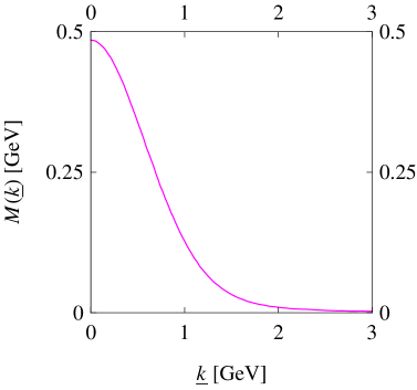
(a)

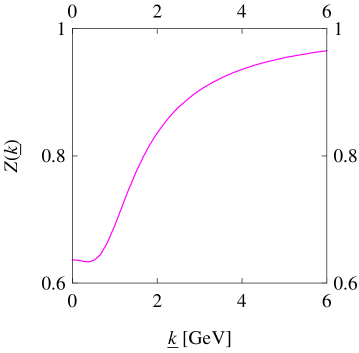
(b)

Figure 1: Dependence, on the Euclidean momentum $\underline{k}$, of both (a) mass function $M(\underline{k})$ and (b) wave-function renormalization function $Z(\underline{k})$ entering in the quark propagator (1) in the chiral limit, extracted and redrawn [2, 4] from Fig. 1 of Ref. [16], emerging as solution to the Dyson–Schwinger equation for the quark two-point Green function imitating the impact of truncated Dyson–Schwinger equations by QCD-inspired ansätze [15].

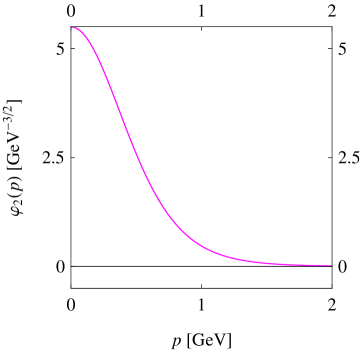
(a)

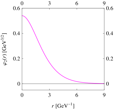
(b)

Figure 2: Nonvanishing radial component function determining the Salpeter amplitude (6) of any massless pseudoscalar quark–antiquark bound state governed by our instantaneous Bethe–Salpeter equation (3) with Fierz-symmetric Dirac structure (4), extracted from the quark propagator functions $M(\underline{k})$ and $Z(\underline{k})$ of Fig. 1, shown in both (a) momentum-space representation, $\varphi_{2}(p)$, and (b) configuration-space representation, $\varphi_{2}(r)$.

Figure 3: Spherically symmetric effective quark–antiquark interaction potential $V(r)$ that upon insertion into our instantaneous Bethe–Salpeter equation (5) trimmed to describe pseudoscalar mesons reproduces, as the ground-state solution to that bound-state problem, the (starting-point) Salpeter component depicted in Fig. 2. Its near flatness close to the origin and steep rise to infinity make $V(r)$ reminiscent of a smoothed square well.

Table 1 presents the very satisfactory outcomes of implementation of the potential of Fig. 3 into our bound-state approach (see, e.g., Refs. [28, 29, 30] for corresponding recent Bethe–Salpeter results).

Table 1: Gell-Mann–Oakes–Renner-required features of pseudoscalar quark–antiquark bound states (masses $\widehat{M}_{B},$ decay constants $f_{B}$ and in-meson condensates ${\mathbb{C}}_{B}$) predicted by Eqs. (5) for the potential $V(r)$ of Fig. 3, and adequate quark masses $m$ compared with the current-quark values $\overline{m}(\mu)$ in modified minimal subtraction.

Constituents	$\widehat{M}_{B}$	$f_{B}$	${\mathbb{C}}_{B}$	$m$	$\overline{m}(2\;\mbox{GeV})$
	$[\mbox{MeV}]$	$[\mbox{MeV}]$	$[\mbox{GeV}^{2}]$	$[\mbox{MeV}]$	$[\mbox{MeV}]$ [27]
chiral quarks	6.8	151	0.585	$0.0059$	—
$u$/$d$ quarks	148.6	155	0.598	$2.85$	$3.5^{+0.5}_{-0.2}$
$s$ quarks	620.7	211	0.799	$51.0$	$95^{+9}_{-3}$

References

- [1] W. Lucha and F. F. Schöberl, J. Phys. G 31 (2005) 1133, arXiv:hep-th/0507281.
- [2] W. Lucha and F. F. Schöberl, Int. J. Mod. Phys. A 31 (2016) 1650202, arXiv:1606.04781 [hep-ph].
- [3] W. Lucha, EPJ Web Conf. 129 (2016) 00047, arXiv:1607.02426 [hep-ph].
- [4] W. Lucha, EPJ Web Conf. 137 (2017) 13009, arXiv:1609.01474 [hep-ph].
- [5] W. Lucha, preprint HEPHY-PUB 1000/18 (2018), arXiv:1807.06245 [hep-ph].
- [6] E. E. Salpeter and H. A. Bethe, Phys. Rev. 84 (1951) 1232.
- [7] E. E. Salpeter, Phys. Rev. 87 (1952) 328.
- [8] W. Lucha and F. F. Schöberl, Phys. Rev. D 87 (2013) 016009, arXiv:1211.4716 [hep-ph].
- [9] W. Lucha, Proc. Sci., EPS-HEP 2013 (2013) 007, arXiv:1308.3130 [hep-ph].
- [10] P. Maris, C. D. Roberts, and P. C. Tandy, Phys. Lett. B 420 (1998) 267, arXiv:nucl-th/9707003.
- [11] W. Lucha and F. F. Schöberl, Phys. Rev. D 92 (2015) 076005, arXiv:1508.02951 [hep-ph].
- [12] W. Lucha and F. F. Schöberl, Phys. Rev. D 93 (2016) 056006, arXiv:1602.02356 [hep-ph].
- [13] W. Lucha and F. F. Schöberl, Phys. Rev. D 93 (2016) 096005, arXiv:1603.08745 [hep-ph].
- [14] W. Lucha and F. F. Schöberl, Int. J. Mod. Phys. A 33 (2018) 1850047, arXiv:1801.00264 [hep-ph].
- [15] P. Maris and P. C. Tandy, Phys. Rev. C 60 (1999) 055214, arXiv:nucl-th/9905056.
- [16] P. Maris, in Proceedings of the International Conference on Quark Confinement and the Hadron Spectrum IV, editors W. Lucha and K. Maung Maung (World Scientific, Singapore, 2002), p. 163, arXiv:nucl-th/0009064.
- [17] Z.-F. Li, W. Lucha, and F. F. Schöberl, Phys. Rev. D 76 (2007) 125028, arXiv:0707.3202 [hep-ph].
- [18] W. Lucha and F. F. Schöberl, Phys. Rev. A 56 (1997) 139, arXiv:hep-ph/9609322.
- [19] W. Lucha and F. F. Schöberl, Int. J. Mod. Phys. A 14 (1999) 2309, arXiv:hep-ph/9812368.
- [20] W. Lucha, K. Maung Maung, and F. F. Schöberl, Phys. Rev. D 63 (2001) 056002, arXiv:hep-ph/0009185.
- [21] W. Lucha, K. Maung Maung, and F. F. Schöberl, Phys. Rev. D 64 (2001) 036007, arXiv:hep-ph/0011235.
- [22] W. Lucha and F. F. Schöberl, Recent Res. Dev. Phys. 5 (2004) 1423, arXiv:hep-ph/0408184.
- [23] W. Lucha and F. F. Schöberl, Int. J. Mod. Phys. A 29 (2014) 1450057, arXiv:1401.5970 [hep-ph].
- [24] W. Lucha and F. F. Schöberl, Int. J. Mod. Phys. A 29 (2014) 1450181, arXiv:1408.4957 [hep-ph].
- [25] W. Lucha and F. F. Schöberl, Int. J. Mod. Phys. A 29 (2014) 1450195, arXiv:1410.5241 [hep-ph].
- [26] M. Gell-Mann, R. J. Oakes, and B. Renner, Phys. Rev. 175 (1968) 2195.
- [27] Particle Data Group (M. Tanabashi et al.), Phys. Rev. D 98 (2018) 030001.
- [28] T. Hilger, M. Gómez-Rocha, A. Krassnigg, and W. Lucha, Eur. Phys. J. A 53 (2017) 213, arXiv:1702.06262 [hep-ph].
- [29] T. Hilger, M. Gómez-Rocha, A. Krassnigg, and W. Lucha, preprint HEPHY-PUB 1003/18 (2018), arXiv:1807.06245 [hep-ph].
- [30] T. Hilger, M. Gómez-Rocha, A. Krassnigg, and W. Lucha, preprint HEPHY-PUB 1008/18 (2018), arXiv:1810.01197 [hep-ph].