Spontaneous emission of a sodium Rydberg atom close to an optical nanofibre

Abstract

We report on numerical calculations of the spontaneous emission rate of a Rydberg-excited sodium atom in the vicinity of an optical nanofibre. In particular, we study how this rate varies with the distance of the atom to the fibre, the fibre’s radius, the symmetry $s$ or $p$ of the Rydberg state as well as its principal quantum number. We find that a fraction of the spontaneously emitted light can be captured and guided along the fibre. This suggests that such a setup could be used for networking atomic ensembles, manipulated in a collective way due to the Rydberg blockade phenomenon.

Keywords: Rydberg atoms, Optical nanofibres, Spontaneous emission rates

1 Introduction

Within the last two decades, the strong dipole-dipole interaction experienced by two neighbouring Rydberg-excited atoms [1] has become the main ingredient for many of the atomic quantum information protocol proposals (see [2] and references therein). In particular, this interaction can be so large as to even forbid the simultaneous resonant excitation of two atoms if their separation is less than a specific distance, called the blockade radius, which typically depends on the intensity of the laser excitation and the interaction between the Rydberg atoms. The discovery of this “Rydberg blockade” phenomenon [3, 4, 5, 6, 7, 8] paved the way for a new encoding scheme using atomic ensembles as collective quantum registers [3, 9, 10, 11] and repeaters [12, 13, 14]. In this novel framework, information is stored in collective spin-wave-like symmetric states, which contain fully delocalized atomic excitations. Qubits are more easily manipulated and more robust in this collective approach than in the usual single-particle paradigm.

Scalability is one of the crucial requirements for quantum devices and interfacing atomic ensembles into a quantum network is a possible way to reach this goal. Photons naturally appear as ideal information carriers and the photon-based protocols considered so far include free-space [15], or guided propagation through optical fibres [12]. The former has the advantage of being relatively easy to implement, but presents the drawback of strong losses. The latter requires a cavity quantum electrodynamics setup, which is experimentally more involved. An alternative option would be to resort to optical nanofibres. Such fibres have recently received much attention [16, 17] because the coupling to the evanescent (resp. guided) modes of a nanofibre allows for easy-to-implement atom trapping [18, 19] (resp. detection [20]). This coupling increases in strength as the fibre diameter reduces and the atoms approach the fibre surface. It was also even shown that energy could be exchanged between two distant atoms via the guided modes of the fibre [21]. This strongly suggests that optical nanofibres could play the role of a communication channel between the nodes of an atomic quantum network consisting of Rydberg-excited atomic ensembles.

In this article, we make a first step towards this goal and investigate the emission rate of a highly-excited (Rydberg) sodium atom in the neighbourhood of an optical nanofibre made of silica. In the perspective of building a quantum network, we are particularly interested in quantifying how much spontaneously emitted light can be captured and guided along the fibre. Here, we study the influence of the atom to fibre distance, the radius of the fibre, and the symmetry of the Rydberg state, on the emission rates into the guided and radiative fibre modes. We find that up to $\approx 13\%$, of the spontaneously emitted light can be captured and guided along both directions of the fibre, which is comparable with the ratio of $\approx 30\%$ obtained with a cesium atom initially in its lowest excited state $6P_{\nicefrac{{3}}{{2}}}$ and located on the surface of a 200-nm-diameter nanofibre [22]. Although the theoretical framework we use here is the same, numerical calculations are more complex than in [22] due to the larger number of transitions considered. Contrary to Ref. [22], we do not take into account the atomic hyperfine structure in the excited state, which is very small for Rydberg states [23].

The article is organized as follows. In Sec. 2 we briefly present the system and introduce the expressions of the spontaneous emission rates. In Sec. 3, we present the results of our numerical calculations and discuss the different behaviours observed when the atom is initially in an $s$ or $p$ Rydberg state. Finally, in Sec. 4, we conclude and give perspectives of our work. A and B provide details about the guided and radiative electromagnetic modes, C sketches the derivation of the spontaneous emission rates of the atom in the presence of the nanofibre and D displays the atomic data we used in our calculations.

2 The system

We consider a sodium atom, initially prepared in the highly-excited (Rydberg) level $n\leq 10$, in the vicinity of a silica nanofibre, whose radius is denoted by $a$ and whose axis is conventionally taken as the $z$-axis (see figure 1). Our goal is to investigate how the presence of the fibre modifies the spontaneous emission rate of the atom : in particular, we want to study the influence of the radius of the fibre, the distance of the atom to the fibre as well as the symmetry of the Rydberg state $\left|nl_{j},m_{j}\right\rangle$ considered and the principal quantum number $n$ on the spontaneous emission rate. Note that, though the configuration is the same as in [22], in this work, the atom is (relatively) highly excited and, in contrast to [22], several transition frequencies must therefore be considered which complicates the numerical work. The choice of the sodium atom and the maximal principal quantum number $n_{\text{max}}=10$ is motivated by the fact that, for the relevant transitions $10\rightarrow n=3,\cdots,9$, the fibre can be approximately considered as a nonabsorbing medium of respective refractive indices $n_{1}=\left(1.467,1.450,1.438,1.399,1.112,1.615,2.021\right)$ [24]. Such constraints may, however, be alleviated by resorting to the formalism of macroscopic quantum electrodynamics and the Green’s function approach [25]. These techniques allow to take the absorption of the medium into account and therefore to deal with higher Rydberg states. This formalism and its application to the calculation of energy shifts will be investigated in a future work. Moreover, the choice of sodium, rather than rubidium or cesium which are more commonly used in nanofibre experiments, was made to allow us to neglect relativistic effects on the electronic wavefunctions and therefore simplify our treatment. The case of cesium will also be tackled in a future work.

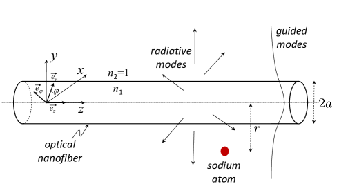
Figure 1: Sodium atom in the vicinity of an optical nanofibre with a radius $a$. The index is $n_{1}=1.45$ for silica and $n_{2}=1$ for vacuum. The axis of the nanofibre is arbitrarily chosen as the $z$-axis. The cylindrical coordinates $\left(r,\varphi,z\right)$ and frame $\left(\vec{e}_{r},\vec{e}_{\varphi},\vec{e}_{z}\right)$ are introduced.

As recalled in [22], the free electromagnetic field in the presence of a cylindrical fibre can be decomposed into guided and radiative modes which respectively correspond to energy propagation along the fibre and radially to it (see A and B).

Guided modes are characterized by their frequency $\omega>0$ and order $m$, which is a positive integer fixing the periodicity of the field with respect to $\varphi$. Due to the continuity conditions at the core-cladding interface of the fibre, the norm of the projection of the wavevector onto the $z$ axis, denoted by $\beta$, can only take a discrete set of values which are the solutions of the so-called characteristic equation equation (3) [26, 27]. The corresponding modes have different cutoff frequencies. In particular, if $\omega$ is sufficiently low, only the (so-called “hybrid”) mode $HE_{11}$, corresponding to $m=1$, can propagate along the fibre. Since a given mode can propagate either in the positive or negative $z$-direction, an extra index $f=\pm 1$ is introduced, such that $\beta\times f$ is the (algebraic) projection of the wavevector onto the $z$-axis. To complete the description, one also allows for two different polarization directions labelled by $p=\pm 1$. For the sake of simplicity, we shall gather the characteristic numbers $\left(\omega,m,f,p\right)$ into one symbol $\mu$ and replace the discrete/continuous sums $\sum_{mfp}\int_{0}^{\infty}d\omega$ by $\sum_{\mu}$. Finally the general form of the quantized guided field component is

$$\vec{E}_{g}\left(\vec{r}\right) = \mathrm{i}\sum_{\mu}\;\sqrt{\frac{\hbar\omega\beta^{\prime}}{4\pi\epsilon_{0}}}a_{\mu}\vec{e}^{\left(\mu\right)}\left(r,\varphi\right)e^{\mathrm{i}\left(f\beta z+p\varphi\right)}+\mbox{h.c.}$$

In this expression, $\beta^{\prime}$ stands for the derivative $\left(\frac{d\beta}{d\omega}\right)$, $\vec{e}_{\mu}$ is the electric-field profile function of the mode $\left(\mu\right)$ whose expression is given in A, while $a_{\mu}$ is the annihilation operator of the mode, satisfying the bosonic commutation rules $\left[a_{\mu},a_{\mu^{\prime}}^{\dagger}\right]=\delta\left(\omega-\omega^{\prime}\right)\delta_{mm^{\prime}}\delta_{ff^{\prime}}\delta_{pp^{\prime}}$.

Radiative modes are characterized by their frequency $\omega>0$, their (positive integer) order $m$ and the projection of the wavevector on the nanofibre axis $\beta$ which can now vary continuously between $-\omega n_{2}/c$ and $\omega n_{2}/c$. Here, the negative or positive sign indicates the direction of the propagation of the radiation mode along the $z$-axis. A last number is needed to fully determine a radiative mode, i.e. the polarization number $p=\pm 1$. The two values of $p$ correspond to two modes of orthogonal polarizations, see B. For the sake of simplicity, we shall gather the characteristic numbers $\left(\omega,\beta,m,p\right)$ into one symbol $\nu$ and replace the discrete/continuous sums $\sum_{mp}\int_{0}^{\infty}d\omega\int_{-kn_{2}}^{kn_{2}}d\beta$ by $\sum_{\nu}$. The general form of the quantized radiative field component is

$$\vec{E}_{r}\left(\vec{r}\right)=\mathrm{i}\sum_{\nu}\;\sqrt{\frac{\hbar\omega}{4\pi\epsilon_{0}}}a_{\nu}\vec{e}^{\left(\nu\right)}\left(r,\varphi\right)e^{\mathrm{i}\left(\beta z+m\varphi\right)}+\mbox{h.c.}$$

In this expression, $\vec{e}_{\nu}$ is the electric-field profile function of the mode $\left(\nu\right)$ whose expression is given in B, while $a_{\nu}$ is the annihilation operator of the mode, satisfying the bosonic commutation rules $\left[a_{\nu},a_{\nu^{\prime}}^{\dagger}\right]=\delta\left(\omega-\omega^{\prime}\right)\delta_{mm^{\prime}}\delta_{pp^{\prime}}$.

In the presence of the nanofibre, the spontaneous emission rate $\Gamma_{M}$ of an atom from a state $\left|M\right\rangle$ is the sum of the rates $\gamma_{MN}$ from $\left|M\right\rangle$ to all lower states $\left|N\right\rangle$, i.e. $\Gamma_{M}\equiv\sum_{N<M}\gamma_{MN}$ with

$$\gamma_{MN}\equiv 2\pi\sum_{\lambda}\left|G_{\lambda MN}\right|^{2}\delta\left(\omega_{\lambda}-\omega_{MN}\right).$$ (1)

In the expression above, the sum is performed over all electromagnetic modes denoted by $\lambda$, whether they be guided $\left(\lambda=\mu\right)$ or radiative $\left(\lambda=\nu\right)$ ; we moreover introduce the quantities

$$G_{\mu MN} \equiv -\sqrt{\frac{\omega\beta^{\prime}}{4\pi\epsilon_{0}\hbar}}\left(\vec{d}_{MN}\cdot\vec{e}^{\left(\mu\right)}\right)e^{\mathrm{i}\left(f\beta z+p\varphi\right)},$$

$$G_{\nu MN} \equiv -\sqrt{\frac{\omega}{4\pi\epsilon_{0}\hbar}}\left(\vec{d}_{MN}\cdot\vec{e}^{\left(\nu\right)}\right)e^{\mathrm{i}\left(\beta z+m\varphi\right)},$$

characterizing the coupling of the different electromagnetic modes to the atomic transition $\left|M\right\rangle\rightarrow\left|N\right\rangle$ of frequency $\omega_{MN}\equiv\nicefrac{{\left(E_{M}-E_{N}\right)}}{{\hbar}}$ and dipole matrix element $\vec{d}_{MN}$. Finally the decoherence rate between states $\left|M\right\rangle$ and $\left|N\right\rangle$ is given by

$$\Gamma_{MN}\equiv\frac{1}{2}\left(\Gamma_{M}+\Gamma_{N}\right).$$ (2)

For a detailed derivation of equations (1,2), see C.

3 Numerical results and discussion

In this section, we present the numerical results we obtained for the spontaneous emission rate of a sodium atom $\left(Z=11\right)$ initially prepared either in $\left|ns_{\nicefrac{{1}}{{2}}},m_{j}\right\rangle$ or $\left|np_{j},m_{j}\right\rangle$ states with $n\leq 10$ and $j=1/2$ or $3/2$. We study the influence of the principal quantum number, $n$, and the distance from the atom to the fibre surface on the emission rate. We also show how the fibre’s radius modifies the relative weights of the different transitions’ contributions to the total rate. For simplicity, we consider the contributions of the guided and radiative modes separately. The atomic data we used can be found in D.

3.1 Guided modes

Figure 2 displays the spontaneous emission rates, $\Gamma_{g}^{10s}$ and $\Gamma_{g}^{10p}$, of an atom initially prepared in the states $\left|10s_{\nicefrac{{1}}{{2}}},m_{j}\right\rangle$ and $\left|10p_{j},m_{j}\right\rangle$ with $j=1/2$ or $3/2$ , respectively, into the guided modes as a function of the distance $r$ to the fibre axis (see figure 1). Note that the rates are presented relative to the spontaneous emission rates $\Gamma_{0}^{10s}$, $\Gamma_{0}^{10p}$ in vacuum and $r$ is expressed in units of the fibre radius with $a=100$ nm. As expected, in both cases, the influence of the guided modes vanishes as $r$ increases, and therefore $\Gamma_{g}^{10s},\Gamma_{g}^{10p}\rightarrow 0$ when $r\rightarrow+\infty$. The maximal value is obtained for $r=a$, i.e. when the atom is on the fibre surface. More precisely, we have $\Gamma_{g}^{10s}\approx 0.18\Gamma_{0}^{10s}$ for an atom initially prepared in $\left|10s_{\nicefrac{{1}}{{2}}},m_{j}=\pm\frac{1}{2}\right\rangle$ and $\Gamma_{g}^{10p}\approx\left(0.027,0.035,0.044\right)\times\Gamma_{0}^{10p}$ for an atom initially prepared in $\left(\left|10p_{\nicefrac{{3}}{{2}}},m_{j}=\pm\frac{1}{2}\right\rangle,\left|10p_{\nicefrac{{1}}{{2}}},m_{j}=\pm\frac{1}{2}\right\rangle,\left|10p_{\nicefrac{{3}}{{2}}},m_{j}=\pm\frac{3}{2}\right\rangle\right)$. In these calculations we assumed that the electronic wave-function of the Rydberg atom is not affected by the nanofibre, which deserves further study. As a more realistic configuration, we shall consider that the Rydberg atom is located at a distance from the fibre surface which is much larger than its radius $r_{Na}\approx 5\text{ nm}=\frac{a}{20}$. For $r=a+10r_{Na}\approx 1.5\times a$, we obtain the spontaneous rate $\Gamma_{g}^{10s}\approx 0.066\times\Gamma_{0}^{10s}$ for an atom initially prepared in $\left|10s_{\nicefrac{{1}}{{2}}},m_{j}=\pm\frac{1}{2}\right\rangle$ and $\Gamma_{g}^{10p}\approx\left(0.006,0.011,0.015\right)\times\Gamma_{0}^{10p}$ for an atom initially prepared in $\left(\left|10p_{\nicefrac{{3}}{{2}}},m_{j}=\pm\frac{1}{2}\right\rangle,\left|10p_{\nicefrac{{1}}{{2}}},m_{j}=\pm\frac{1}{2}\right\rangle,\left|10p_{\nicefrac{{3}}{{2}}},m_{j}=\pm\frac{3}{2}\right\rangle\right)$. Moreover, we note that in general, $\Gamma_{g}^{10p}\ll\Gamma_{g}^{10s}$, and $\Gamma_{g}^{10p_{\nicefrac{{3}}{{2}}},m_{j}=\pm\frac{1}{2}}<\Gamma_{g}^{10p_{\nicefrac{{1}}{{2}}}}<\Gamma_{g}^{10p_{\nicefrac{{3}}{{2}}},m_{j}=\pm\frac{3}{2}}$. The latter relation can be qualitatively understood by geometric arguments on the coupling of guided modes with the atomic orbitals. The more a state is polarized along $z$, the less it couples to the guided modes which are essentially polarized orthogonally to the fibre axis. This is consistent with what we observe, since the states $\left|10p_{\nicefrac{{3}}{{2}}},m_{j}=\pm\frac{1}{2}\right\rangle$ are better aligned along $z$ than the states $\left|10p_{\nicefrac{{1}}{{2}}},m_{j}=\pm\frac{1}{2}\right\rangle$ which themselves are more aligned along $z$ than $\left|10p_{\nicefrac{{3}}{{2}}},m_{j}=\pm\frac{3}{2}\right\rangle$. This can be seen on their relation with the decoupled basis states [29].

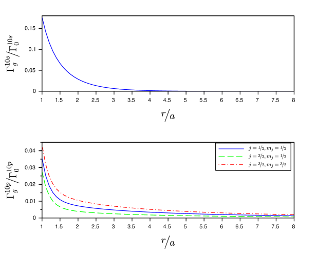
Figure 2: Spontaneous emission rate of a sodium atom into the guided modes of a nanofibre of radius $a=100$nm. The rate is plotted as a function of the distance $r$ of the atom to the fibre axis : (top) atom initially prepared in the state $\left|10s_{\nicefrac{{1}}{{2}}},m_{j}=\pm\frac{1}{2}\right\rangle$, (bottom) atom initially prepared in the states $\left|10p_{\nicefrac{{1}}{{2}}},m_{j}=\pm\frac{1}{2}\right\rangle$, $\left|10p_{\nicefrac{{3}}{{2}}},m_{j}=\pm\frac{1}{2}\right\rangle$ and $\left|10p_{\nicefrac{{3}}{{2}}},m_{j}=\pm\frac{3}{2}\right\rangle$. The rates $\Gamma_{g}^{10s},\Gamma_{g}^{10p}$ are presented relative to the spontaneous emission rates $\Gamma_{0}^{10s}$, $\Gamma_{0}^{10p}$ in vacuum.

Figure 3 shows the influence of the principal quantum number $n$ on the spontaneous emission rate $\Gamma_{g}^{ns}$ into the guided modes for an atom initially prepared in the state $\left|ns_{\nicefrac{{1}}{{2}}},m_{j}=\pm\frac{1}{2}\right\rangle$ for $n=5$ to $10$. The higher the value of $n$, the more $\Gamma_{g}^{ns}$ is peaked as a function of $r/a$ around $1$. Moreover, the plots get closer and closer as $n$ increases : the curves $n=9,10$ cannot be distinguished and for the sake of clarity, the curve $n=8$ has not been plotted.

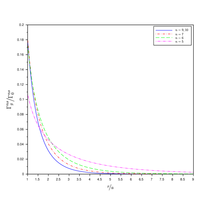
Figure 3: Spontaneous emission rate of a sodium atom initially prepared in $\left|ns_{\nicefrac{{1}}{{2}}},m_{j}=\pm\frac{1}{2}\right\rangle$, for $n=5,\cdots,10$, into the guided modes of a nanofibre of radius $a=100$ nm. The rate is plotted as a function of the distance $r$ of the atom from the fibre axis. The rate, $\Gamma_{g}^{ns}$, is renormalized by the spontaneous emission rate in vacuum, $\Gamma_{0}^{ns}$, and the distance $r$ is expressed in units of the fibre radius, $a$.

Finally, figures 4 and 5 illustrate the influence of the fibre radius, $a$, on the spontaneous emission rate from the state $\left|ns_{\nicefrac{{1}}{{2}}},m_{j}=\pm\frac{1}{2}\right\rangle$ into the guided modes. More precisely, figure 4 displays the partial spontaneous emission rates along the specific transition $10s\rightarrow 3p$ (Note that $n=3$ corresponds to the ground state of the sodium atom) into different guided modes $HE_{mn}$, $EH_{mn}$, $TE_{mn}$ and $TM_{mn}$. Two cases are considered : (i) the atom is located on the fibre surface, i.e. at a distance $r=a$ from the $z$-axis, and (ii) the atom is placed at a fixed distance of $150$ nm from the fibre surface, i.e. at a distance $r=a+150\text{ nm}$ from the $z$-axis. As expected, case (ii) gives rise to much weaker relative rates than case (i), since the atom is further away from the fibre and therefore the guided modes are strongly attenuated. Moreover, as $a$ increases, the cutoff frequencies of higher modes become smaller : when the cutoff frequency of one mode passes below the frequency of the transition $10s\rightarrow 3p$, this mode starts to contribute to the spontaneous emission rate. The peaked structure observed on the different plots results from the peaked shape of the mode intensity profile itself with respect to $a$.

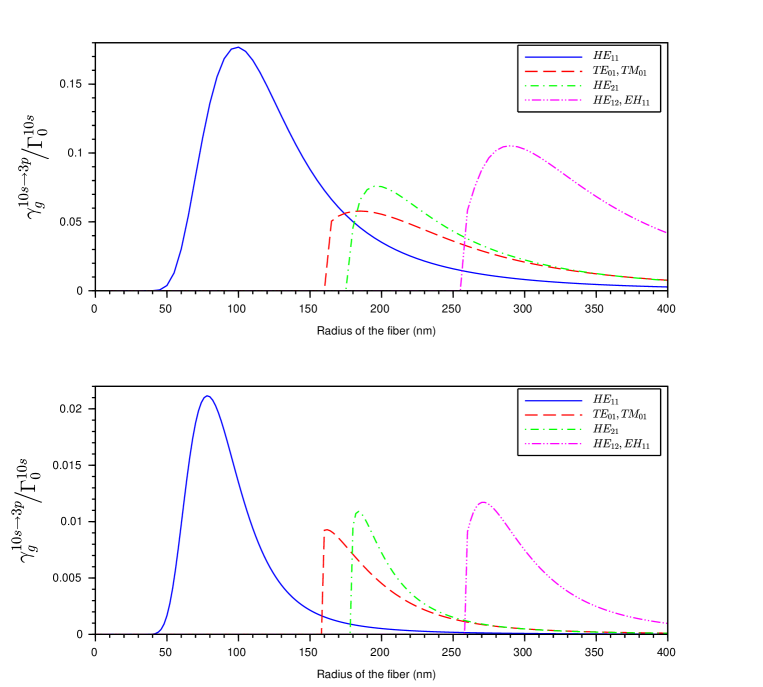
Figure 4: Partial spontaneous emission rates of a sodium atom along the specific transition $10s\rightarrow 3p$ into different guided modes of the nanofiber, as functions of the fibre radius, $a$ : (top) the atom is on the fibre surface ; (bottom) the atom is located at a distance $150$ nm from the fibre surface. The rates are presented relative to the spontaneous emission rate in vacuum, $\Gamma_{0}^{10s}$.

Figure 5 displays the partial spontaneous emission rates $\gamma_{g}^{10s\rightarrow np}$ into the guided modes along the respective transitions $10s\rightarrow np$ as well as the total rate $\Gamma_{g}^{10s}=\sum_{3\leq n\leq 10}\gamma_{g}^{10s\rightarrow np}$ as functions of the fibre radius, $a$, in the same two cases (i, ii) as above. One observes that, due to the range chosen for $a$, only the transitions $10s\rightarrow np$ for $n=3,4,5$ give relevant contributions to the total rate. It also appears that only the transition $10s\rightarrow 3p$ substantially couples to higher-order guided modes, while the other transitions couple only to the fundamental guided mode $HE_{11}$. On the range chosen for $a$, the peak structure observed for the total emission rate is therefore mainly due to the partial rate $\gamma_{g}^{10s\rightarrow 3p}$, while the other transitions smoothly modify the value of $\Gamma_{g}^{10s}$. Note that the intensity profiles of the guided modes relative to the different transition frequencies are expected to coincide up to a rescaling of the $a$-axis : this scaling factor is given by the ratio of the frequencies. The positions of the peaks of the different partial rates $\gamma_{g}^{10s\rightarrow np}$ should therefore also coincide up to a simple scaling. The heights of the peaks, however, are expected to be different since, for instance, the dipole matrix element is not the same for the different transitions.

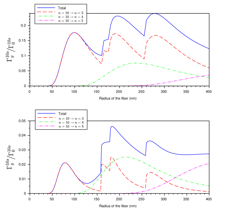
Figure 5: Partial, $\gamma_{g}^{10s\rightarrow np}$, and total, $\Gamma_{g}^{10s}$, spontaneous emission rates of a sodium atom initially prepared in $\left|10s_{\nicefrac{{1}}{{2}}},m_{j}=\pm\frac{1}{2}\right\rangle$ into the guided modes of a nanofibre. The rates are plotted as a function of the fibre radius, $a$ : (top) the atom is on the fibre surface ; (bottom) the atom is located at a distance $150$ nm from the fibre surface. The rates are presented relative to the spontaneous emission rate in vacuum, $\Gamma_{0}^{10s}$.

3.2 Radiative modes

We now turn to the contribution of the radiative modes to the total spontaneous emission rates. Figure 6 displays the spontaneous emission rates $\Gamma_{r}^{10s}$ and $\Gamma_{r}^{10p}$ of an atom initially prepared in the states $\left|10s_{\nicefrac{{1}}{{2}}},m_{j}\right\rangle$, $\left|10p_{\nicefrac{{1}}{{2}},\nicefrac{{3}}{{2}}},m_{j}\right\rangle$, respectively into the radiative modes as a function of the distance $r$ to the fibre axis (see figure 1). Note that the rates are renormalized by the spontaneous emission rates in vacuum $\Gamma_{0}^{10s}$, resp. $\Gamma_{0}^{10p}$, and $r$ is expressed in units of the fibre radius $a=100$ nm. As expected, in both cases, the influence of the fibre vanishes as $r$ increases, i.e. $\Gamma_{r}^{10s},\Gamma_{r}^{10p}\rightarrow 1$ for $r\rightarrow+\infty$. The maximal value is observed for $r=a$, i.e. when the atom is on the fibre surface. More precisely, we have $\Gamma_{r}^{10s}\approx 1.24\times\Gamma_{0}^{10s}$ for an atom initially prepared in $\left|10s_{\nicefrac{{1}}{{2}}},m_{j}=\pm\frac{1}{2}\right\rangle$ and $\Gamma_{r}^{10p}\approx\left(1.19,1.23,1.29\right)\times\Gamma_{0}^{10p}$ for an atom initially prepared in $\left(\left|10p_{\nicefrac{{3}}{{2}}},m_{j}=\pm\frac{1}{2}\right\rangle,\left|10p_{\nicefrac{{1}}{{2}}},m_{j}=\pm\frac{1}{2}\right\rangle,\left|10p_{\nicefrac{{3}}{{2}}},m_{j}=\pm\frac{3}{2}\right\rangle\right)$. For an atom at $r\approx 1.5\times a$, , i.e., at a distance from the fibre surface, we obtain the spontaneous rate $\Gamma_{r}^{10s}\approx 1.041\times\Gamma_{0}^{10s}$ for an atom initially prepared in $\left|10s_{\nicefrac{{1}}{{2}}},m_{j}=\pm\frac{1}{2}\right\rangle$ and $\Gamma_{r}^{10p}\approx\left(1.028,1.044,1.062\right)\times\Gamma_{0}^{10p}$ for an atom initially prepared in $\left(\left|10p_{\nicefrac{{3}}{{2}}},m_{j}=\pm\frac{1}{2}\right\rangle,\left|10p_{\nicefrac{{1}}{{2}}},m_{j}=\pm\frac{1}{2}\right\rangle,\left|10p_{\nicefrac{{3}}{{2}}},m_{j}=\pm\frac{3}{2}\right\rangle\right)$. This allows us to compute the proportion of light which is emitted into the guided and radiative modes. For instance, for an atom initially prepared in the state $\left|10s_{\nicefrac{{1}}{{2}}},m_{j}=\pm\frac{1}{2}\right\rangle$, $\Gamma_{g}/\left(\Gamma_{g}+\Gamma_{r}\right)\approx 13\%$ when the atom is located on the fibre surface $\left(r=a\right)$, and $\Gamma_{g}/\left(\Gamma_{g}+\Gamma_{r}\right)\approx 6\%$ when the atom is located at $50$ nm from the fibre surface $\left(r=1.5\times a\right)$. Since light is mostly spontaneously emitted into the radiative modes, it seems quite challenging to efficiently interface a Rydberg atom with a guided mode of the nanofibre and, thence, to build a valuable quantum network. The use of atomic ensembles might alleviate this concern, since, as already demonstrated in free-space, their spontaneous emission could be made highly directional and their coupling strength is enhanced [15]. These issues and the perspectives they offer will be addressed in a future work.

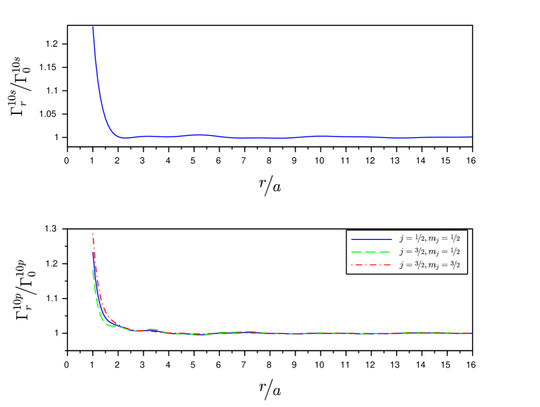
Figure 6: Total spontaneous emission rate of a sodium atom into the radiative modes of a nanofibre of radius $a=100$ nm. The rate is plotted as a function of the distance $r$ of the atom to the fibre axis : (top) atom initially prepared in the state $\left|10s_{\nicefrac{{1}}{{2}}},m_{j}=\pm\frac{1}{2}\right\rangle$, (bottom) atom initially prepared in the states $\left|10p_{\nicefrac{{1}}{{2}}},m_{j}=\pm\frac{1}{2}\right\rangle$, $\left|10p_{\nicefrac{{3}}{{2}}},m_{j}=\pm\frac{1}{2}\right\rangle$ and $\left|10p_{\nicefrac{{3}}{{2}}},m_{j}=\pm\frac{3}{2}\right\rangle$. The rates $\Gamma_{r}^{10s},\Gamma_{r}^{10p}$ are presented relative to the spontaneous emission rates $\Gamma_{0}^{10s}$, $\Gamma_{0}^{10p}$ in vacuum and the distance $r$ is expressed in units of the fibre radius, $a$.

Finally, in figure 6, one observes a damped semi-oscillatory behaviour for $\Gamma_{r}^{10s}$ and $\Gamma_{r}^{10p}$ as functions of $r$, and for $\Gamma_{r}^{10p}$ the oscillations of the different contributions $j=1/2,3/2$ are not in phase. These features result from the behaviour of the different transition components $\gamma_{nl\rightarrow n^{\prime}l^{\prime}}$ shown in figure 7 for $nl=np_{\nicefrac{{3}}{{2}}},m_{j}=\pm\frac{1}{2}$, which is itself due to the oscillatory behaviour of the radiative field. For a transition of frequency $\omega$, the frequency of oscillation with $r$ is approximately given by $2\omega/c$.

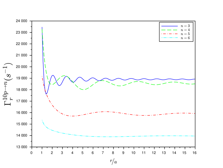
Figure 7: Spontaneous emission rate of a sodium atom initially prepared in $\left|10p_{\nicefrac{{3}}{{2}}},m_{j}=\pm\frac{1}{2}\right\rangle$ into the radiative modes of a nanofibre of radius $a=100$ nm : contributions of the different transitions $\left|10p_{\nicefrac{{3}}{{2}}},m_{j}=\pm\frac{1}{2}\right\rangle\rightarrow\left|ns_{\nicefrac{{1}}{{2}}},m_{j}=\pm\frac{1}{2}\right\rangle,\left|nd_{\nicefrac{{5}}{{2}}},m_{j}=\pm\frac{1}{2},\pm\frac{3}{2}\right\rangle$, for $n=3,\cdots,6$, . The rate is plotted as a function of the distance $r$ of the atom to the fibre axis. The distance $r$ is expressed in units of the fibre radius, $a$.

4 Conclusion

We have investigated the influence of an optical nanofibre on the spontaneous emission rate of a sodium atom prepared in a Rydberg state. The respective contributions of the guided and radiative modes to the total rate were numerically determined, for different principal quantum numbers and different symmetries, and their remarkable features were physically discussed.

Though the radiative modes’ contribution is dominant, a small fraction of the spontaneously emitted light is transferred into the guided mode of the nanofibre. This effect might be enhanced by resorting to atomic ensembles which could offer stronger and more directional collective coupling. Using thicker fibres, with more than one guided mode, may also yield for a higher ratio of spontaneous emission into the guided modes. This potentially paves the way towards the implementation of a quantum network based on Rydberg atomic ensembles linked by nanofibres, which will be further addressed in a future work.

Appendix A Guided modes

A guided mode is characterized by a set $\mu\equiv\left(\omega,\beta,m,f=\pm,p=\pm\right)$. $\beta$ is the projection of the wavevector onto the axis of the nanofibre whose value is determined by the eigenvalue equation

$$\left(\frac{n_{1}^{2}J_{m}^{\prime}(\kappa a)}{a\kappa J_{m}(\kappa a)}+\frac{n_{2}^{2}K_{m}^{\prime}(\gamma a)}{a\gamma K_{m}(\kappa a)}\right)\left(\frac{J_{m}^{\prime}(\kappa a)}{a\kappa J_{m}(\kappa a)}+\frac{K_{m}^{\prime}(\gamma a)}{a\gamma K_{m}(\gamma a)}\right)$$

$$=\left(\frac{mc\beta}{\omega}\right)^{2}\left(\frac{1}{\left(\gamma a\right)^{2}}+\frac{1}{\left(\kappa a\right)^{2}}\right)^{2}.$$ (3)

Here we introduced $\kappa\equiv\sqrt{n_{1}^{2}k^{2}-\beta^{2}}$, $\gamma\equiv\sqrt{\beta^{2}-n_{2}^{2}k^{2}}$ and $k\equiv\frac{\omega}{c}$. $a$ is the radius of the fibre, $n_{1}$ is the core index, $n_{2}\approx 1$ is the index of the surrounding vacuum. $J_{m}$ and $K_{m}$ denote the Bessel functions of the first kind and the modified Bessel functions of the second kind, respectively. Note that, when the monomode conditions are fulfilled, only the hybrid modes $HE_{11}$ with $m=1$ exist, and are fully characterized by $\mu\equiv\left(\omega,f,p\right)$.

The polarization vectors of the guided mode $\left(\mu\right)$ for $r<a$ are given by

$$e_{r}^{\left(\mu\right)} = \frac{\beta C}{2\textrm{i}\kappa}\frac{K_{m}(\gamma a)}{J_{m}(\kappa a)}\Big{(}J_{m-1}(\kappa r)(1-ms)-J_{m+1}(\kappa r)(1+ms)\Big{)}$$

$$e_{\varphi}^{\left(\mu\right)} = \frac{p\beta C}{2\kappa}\frac{K_{m}(\gamma a)}{J_{m}(\kappa a)}\Big{(}J_{m-1}(\kappa r)(1-ms)+J_{m+1}(\kappa r)(1+ms)\Big{)},$$

$$e_{z}^{\left(\mu\right)} = C\frac{K_{m}(\gamma a)}{J_{m}(\kappa a)}J_{m}(\kappa r),$$

while, for $r>a$, they are

$$e_{r}^{\left(\mu\right)} = \frac{\beta C}{2\textrm{i}\gamma}\Big{(}K_{m-1}(\gamma r)(1-ms)+K_{m+1}(\gamma r)(1+ms)\Big{)},$$

$$e_{\varphi}^{\left(\mu\right)} = \frac{\beta pC}{2\gamma}\Big{(}K_{m-1}(\gamma r)(1-ms)-K_{m+1}(\gamma r)(1+ms)\Big{)},$$

$$e_{z}^{\left(\mu\right)} = CK_{m}(\gamma r),$$

where

$$s=\frac{\frac{1}{\gamma^{2}a^{2}}+\frac{1}{\kappa^{2}a^{2}}}{\frac{J_{m}^{\prime}(\kappa a)}{\kappa aJ_{m}(\kappa a)}+\frac{K_{m}^{\prime}(\gamma a)}{\gamma aK_{m}(\gamma a)}}.$$

Using the normalization condition

$$\int_{0}^{2\pi}\mathrm{d}\varphi\int_{0}^{+\infty}n\left(r\right)^{2}\left|{\bf e}^{\left(\mu\right)}\right|^{2}\leavevmode\nobreak\ r\mathrm{d}r=1,$$

we deduce that

$$|C| = \frac{2}{a\beta K_{m}\left(\gamma a\right)\sqrt{2\pi(n_{1}^{2}A_{1}+n_{2}^{2}A_{2})}}$$

with the abbreviations

$$A_{1} = \left(\frac{1}{\kappa J_{m}\left(\kappa a\right)}\right)^{2}\times\left(\left(1-ms\right)^{2}\left(J_{m-1}^{2}\left(\gamma a\right)-J_{m}\left(\gamma a\right)J_{m-2}\left(\gamma a\right)\right)\right.$$

$$+(1+ms)^{2}\left(J_{m+1}^{2}\left(\gamma a\right)-J_{m}\left(\gamma a\right)J_{m+2}\left(\gamma a\right)\right)$$

$$\left.+2\frac{\kappa^{2}}{\beta^{2}}\left(J_{m}^{2}\left(\gamma a\right)-J_{m-1}\left(\gamma a\right)J_{m+1}\left(\gamma a\right)\right)\right),$$

$$A_{2} = \left(\frac{1}{\gamma K_{m}\left(\gamma a\right)}\right)^{2}\times\left(\left(1-ms\right)^{2}\left(-K_{m-1}^{2}\left(\gamma a\right)+K_{m}\left(\gamma a\right)K_{m-2}\left(\gamma a\right)\right)\right.$$

$$+\left(1+ms\right)^{2}\left(-K_{m+1}^{2}\left(\gamma a\right)+K_{m}\left(\gamma a\right)K_{m+2}\left(\gamma a\right)\right)$$

$$\left.+2\left(\frac{\gamma}{\beta}\right)^{2}\left(-K_{m}^{2}\left(\gamma a\right)+K_{m-1}\left(\gamma a\right)K_{m+1}\left(\gamma a\right)\right)\right).$$

Appendix B Radiative modes

A radiative mode is characterized by a set $\nu\equiv\left(\omega,\beta,m,p=\pm\right)$, where $m$ is the order of the mode, and the meaning of $p$ will be explained below.

Defining the quantities $\kappa\equiv\sqrt{n_{1}^{2}k^{2}-\beta^{2}}$, $\sigma\equiv\sqrt{n_{2}^{2}k^{2}-\beta^{2}}$ and $k\equiv\omega/c$, one can write the polarization vectors of the radiative mode $\left(\nu\right)$ for $r<a$ :

$$e_{r}^{\left(\nu\right)} = \frac{1}{\textrm{i}\kappa}\Big{(}\beta AJ_{m}^{\prime}(\kappa r)+\mathrm{i}B\frac{\omega m}{r\kappa}J_{m}(\kappa r)\Big{)},$$

$$e_{\varphi}^{\left(\nu\right)} = \frac{1}{\textrm{i}\kappa}\Big{(}\mathrm{i}A\frac{m\beta}{\kappa r}J_{m}(\kappa r)-\omega BJ_{m}^{\prime}(\kappa r)\Big{)},$$

$$e_{z}^{\left(\nu\right)} = AJ_{m}(\kappa r),$$

while for $r>a$ :

$$e_{r}^{\left(\nu\right)} = \frac{1}{\textrm{i}\sigma}\left[\beta\left(CJ_{m}^{\prime}(\sigma r)+EY_{m}^{\prime}(\sigma r)\right)+\frac{\mathrm{i}m\omega}{\sigma r}\left(DJ_{m}\left(\sigma r\right)+FY_{m}\left(\sigma r\right)\right)\right],$$

$$e_{\varphi}^{\left(\nu\right)} = \frac{1}{\textrm{i}\sigma}\left[\mathrm{i}\frac{\nu\beta}{\sigma r}\left(CJ_{m}\left(\sigma r\right)+EY_{m}\left(\sigma r\right)\right)-\omega\left(DJ_{m}^{\prime}(\sigma r)+FY_{m}^{\prime}(\sigma r)\right)\right],$$

$$e_{z}^{\left(\nu\right)} = CJ_{m}\left(\sigma r\right)+EY_{m}\left(\sigma r\right),$$

where $Y_{m}$ denote Bessel functions of the second kind. The coefficients $C$, $D$, $E$ and $F$ are related to $A$ and $B$ as follows

$$C = -\frac{\pi a\sigma^{2}}{2\epsilon_{0}n_{2}^{2}}\left(AL_{2}+\textrm{i}BV_{2}\right),$$

$$D = \textrm{i}\frac{\pi a\sigma^{2}}{2}\left(A\mu_{0}V_{2}+\textrm{i}BM_{2}\right),$$

$$E = \frac{\pi a\sigma^{2}}{2\epsilon_{0}n_{2}^{2}}\left(AL_{1}+\textrm{i}BV_{1}\right),$$

$$F = -\textrm{i}\frac{\pi a\sigma^{2}}{2}\left(A\mu_{0}V_{1}+\textrm{i}BM_{1}\right),$$

with

$$V_{1} = \frac{m\beta}{a\omega\mu_{0}\kappa^{2}\sigma^{2}}\left(n_{2}^{2}-n_{1}^{2}\right)J_{m}\left(\sigma a\right)J_{m}\left(\kappa a\right),$$

$$V_{2} = \frac{m\beta}{a\omega\mu_{0}\kappa^{2}\sigma^{2}}\left(n_{2}^{2}-n_{1}^{2}\right)Y_{m}\left(\sigma a\right)J_{m}\left(\kappa a\right),$$

$$M_{1} = \frac{1}{\kappa}J_{m}\left(\sigma a\right)J_{m}^{\prime}\left(\kappa a\right)-\frac{1}{\sigma}J_{m}^{\prime}\left(\sigma a\right)J_{m}\left(\kappa a\right),$$

$$M_{2} = \frac{1}{\kappa}Y_{m}\left(\sigma a\right)J_{m}^{\prime}\left(\kappa a\right)-\frac{1}{\sigma}Y_{m}^{\prime}\left(\sigma a\right)J_{m}\left(\kappa a\right),$$

$$L_{1} = \frac{\epsilon_{0}n_{1}^{2}}{\kappa}J_{m}\left(\sigma a\right)J_{m}^{\prime}\left(\kappa a\right)-\frac{\epsilon_{0}n_{2}^{2}}{\sigma}J_{m}^{\prime}\left(\sigma a\right)J_{m}\left(\kappa a\right),$$

$$L_{2} = \frac{\epsilon_{0}n_{1}^{2}}{\kappa}Y_{m}\left(\sigma a\right)J_{m}^{\prime}\left(\kappa a\right)-\frac{\epsilon_{0}n_{2}^{2}}{\sigma}Y_{m}^{\prime}\left(\sigma a\right)J_{m}\left(\kappa a\right).$$

In the single-mode approximation, a guided mode is completely specified by the frequency $\omega$, the direction of propagation $f=\pm 1$ and the polarization $p=\pm 1$. By contrast, at first glance, this is not the case for the radiative modes any longer. Once $\beta$, $\omega$ and $m$ are fixed, we are left with 2 constants $A$ and $B$, and a normalization condition will only determine one constant. We must therefore separate these into two modes. For instance, we can just set $A=0$ for one mode and $B=0$ for the other one. We want, however, the two modes to be orthogonal to each other. An alternative method consists in setting $B=p\mathrm{i}\eta A$ with the parameter $p=\pm 1$, then imposing an orthogonality condition between ${\bf e}^{\left(p=+1\right)}$ and ${\bf e}^{\left(p=-1\right)}$. Explicitly, this condition is written :

$$\int_{0}^{2\pi}d\varphi\int_{0}^{\infty}n\left(r\right)^{2}\left[{\bf e}^{\left(\nu\right)}\cdot{\bf e}^{\left(\nu^{\prime}\right)}\right]rdr = \delta_{pp^{\prime}}\delta_{mm^{\prime}}\delta\left(\omega-\omega^{\prime}\right)\delta\left(\beta-\beta^{\prime}\right).$$

If we consider the vacuum surrounding with the index $n_{2}=1$, this leads to :

$$\eta = \sqrt{\frac{L_{1}^{2}+L_{2}^{2}+\epsilon_{0}\mu_{0}\left(V_{1}^{2}+V_{2}^{2}\right)}{V_{1}^{2}+V_{2}^{2}+\frac{\epsilon_{0}}{\mu_{0}}\left(M_{1}^{2}+M_{2}^{2}\right)}},$$

$$1 = \frac{2\pi\omega}{\sigma^{2}}\left[\left(\left|C\right|^{2}+\left|E\right|^{2}\right)+c^{2}\left(\left|D\right|^{2}+\left|F\right|^{2}\right)\right].$$

The second normalization equation allows us to calculate the form of $\left|A\right|$

$$\left|A\right|=\frac{1}{\sigma a}\left[\frac{2}{\omega\pi^{3}}\sum_{j=1,2}\left(\frac{1}{\epsilon_{0}}\left|L_{j}-p\eta V_{j}\right|^{2}+\left|\mu_{0}V_{j}-p\eta M_{j}\right|^{2}\right)\right]^{-\frac{1}{2}}.$$

This shows that $\nu=\left(\omega,\beta,m,p\right)$ completely determines a radiative mode.

Appendix C Spontaneous emission of an atom in the presence of a nanofibre

With the definitions $\sigma_{MN}\equiv\left|M\right\rangle\left\langle N\right|$, $\omega_{MN}\equiv\left(E_{M}-E_{N}\right)/\hbar$, $k\equiv\omega/c$, the Hamiltonian of the full system consisting of the atom and the electric field takes the form $H=H_{at}+H_{f}+H_{int}$ with

$$H_{f} = \sum_{\mu}\hbar\omega a_{\mu}^{\dagger}a_{\mu}+\sum_{\nu}\hbar\omega a_{\nu}^{\dagger}a_{\nu},$$

$$H_{at} = \sum_{m}\hbar\omega_{M}\sigma_{MM},$$

$$H_{int} = -\vec{D}\cdot\vec{E},$$

where $\vec{D}=\sum_{M,N}\vec{d}_{MN}\sigma_{MN}$ and $\vec{E}\left(\vec{r}\right)=\vec{E}_{g}\left(\vec{r}\right)+\vec{E}_{r}\left(\vec{r}\right)$ are the atomic dipole operator and the total electric field operator, respectively. Switching to the interaction picture relative to $H_{0}\equiv H_{at}+H_{f}$, and resorting to the rotating wave approximation (RWA) we get the interaction Hamiltonian (note that the states $\left|M\right\rangle$ are ordered by increasing energies)

$$\tilde{H}_{int}\left(t\right) \approx \mathrm{i}\hbar\sum_{N<M}\sum_{\mu}\;G_{\mu MN}\sigma_{MN}a_{\mu}e^{-\mathrm{i}\left(\omega-\omega_{MN}\right)t}+\mathrm{h.c.}$$

$$+\mathrm{i}\hbar\sum_{N<M}\sum_{\nu}\;G_{\nu MN}\sigma_{MN}a_{\nu}e^{-\mathrm{i}\left(\omega-\omega_{MN}\right)t}+\mathrm{h.c.}$$

where we introduced

$$G_{\mu MN} \equiv -\sqrt{\frac{\omega\beta^{\prime}}{4\pi\epsilon_{0}\hbar}}\left(\vec{d}_{MN}\cdot\vec{e}^{\left(\mu\right)}\right)e^{\mathrm{i}\left(f\beta z+p\varphi\right)},$$

$$G_{\nu MN} \equiv -\sqrt{\frac{\omega}{4\pi\epsilon_{0}\hbar}}\left(\vec{d}_{MN}\cdot\vec{e}^{\left(\nu\right)}\right)e^{\mathrm{i}\left(\beta z+m\varphi\right)},$$

For simplicity, from now on we shall use $\lambda$ to denote either guided modes, i.e. $\lambda=\left(\omega,f=\pm,p=\pm\right)$, or radiative modes, i.e. $\lambda=\left(\omega,\beta,m,p\right)$, and use $\sum_{\lambda}$ to represent the sum, either discrete or continuous, of these modes, whence

$$\tilde{H}_{int}\left(t\right) \approx \mathrm{i}\hbar\sum_{N<M}\sum_{\lambda}\;G_{\lambda MN}\sigma_{MN}a_{\lambda}e^{-\mathrm{i}\left(\omega_{\lambda}-\omega_{MN}\right)t}$$ (4)

$$-\mathrm{i}\hbar\sum_{N<M}\sum_{\lambda}\;G_{\lambda MN}^{*}a_{\lambda}^{\dagger}\sigma_{NM}e^{+\mathrm{i}\left(\omega_{\lambda}-\omega_{MN}\right)t}$$

From equation (4), we get the Heisenberg equations for the field and atomic operators, $a_{\lambda}$ and $\sigma_{PQ}$

$$\partial_{t}a_{\lambda} = -\sum_{N<M}\;G_{\lambda MN}^{*}\sigma_{NM}e^{+\mathrm{i}\left(\omega_{\lambda}-\omega_{MN}\right)t},$$ (5)

$$\partial_{t}\sigma_{PQ} = \sum_{M<Q}\sum_{\lambda}\;G_{\lambda QM}\sigma_{PM}\left(t\right)a_{\lambda}\left(t\right)e^{-\mathrm{i}\left(\omega_{\lambda}-\omega_{QM}\right)t}$$ (6)

$$-\sum_{P<M}\sum_{\lambda}\;G_{\lambda MP}\sigma_{MQ}\left(t\right)a_{\lambda}\left(t\right)e^{-\mathrm{i}\left(\omega_{\lambda}-\omega_{MP}\right)t}$$

$$-\sum_{Q<M}\sum_{\lambda}\;G_{\lambda MQ}^{*}a_{\lambda}^{\dagger}\left(t\right)\sigma_{PM}\left(t\right)e^{+\mathrm{i}\left(\omega_{\lambda}-\omega_{MQ}\right)t}$$

$$+\sum_{M<P}\sum_{\lambda}\;G_{\lambda PM}^{*}a_{\lambda}^{\dagger}\left(t\right)\sigma_{MQ}\left(t\right)e^{+\mathrm{i}\left(\omega_{\lambda}-\omega_{PM}\right)t}.$$

We can eliminate the field degree of freedom by inserting the formal solution of equation (5)

$$a_{\lambda}\left(t\right) = a_{\lambda}\left(t_{0}\right)-\sum_{N<M}\;G_{\lambda MN}^{*}\int_{t_{0}}^{t}\sigma_{NM}\left(s\right)e^{+\mathrm{i}\left(\omega_{\lambda}-\omega_{MN}\right)s}$$

into equation (6). Then performing Markov approximation [28] and using

$$\int_{0}^{\infty}dse^{\pm\mathrm{i}\Delta s} = \pi\delta\left(\Delta\right)\pm\mathrm{i}\mathcal{P}\left(\frac{1}{\Delta}\right)$$

we get

$$\partial_{t}\sigma_{PQ} \approx -\left\{\Gamma_{PQ}+\mathrm{i}\Delta_{PQ}\right\}\sigma_{PQ}\left(t\right)+\delta_{PQ}\sum_{P<M}\gamma_{MP}\sigma_{MM}\left(t\right)+\xi_{PQ}\left(t\right)$$

where we introduced the different decay rates and energy shifts due to spontaneous emission into the modes of the fibre,

$$\Gamma_{PQ} \equiv \frac{1}{2}\left(\Gamma_{P}+\Gamma_{Q}\right)$$

$$\Delta_{PQ} \equiv \Delta_{P}-\Delta_{Q}$$

$$\Gamma_{P} \equiv \sum_{M<P}\gamma_{PM}$$

$$\gamma_{PQ} \equiv 2\pi\sum_{\lambda}\left|G_{\lambda PQ}\right|^{2}\delta\left(\omega_{\lambda}-\omega_{PQ}\right)$$

$$\Delta_{P} \equiv \mathcal{P}\left(\sum_{M<P}\sum_{\lambda}\frac{\left|G_{\lambda PM}\right|^{2}}{\omega_{\lambda}-\omega_{PM}}-\frac{\left|G_{\lambda PM}^{\left(0\right)}\right|^{2}}{\omega_{\lambda}-\omega_{PM}}\right)+\Delta_{P}^{\left(0\right)}$$

and the associated Langevin forces

$$\xi_{PQ}\left(t\right) \equiv \sum_{M<Q}\sum_{\lambda}\;G_{\lambda QM}\sigma_{PM}\left(t\right)a_{\lambda}\left(t_{0}\right)e^{-\mathrm{i}\left(\omega_{\lambda}-\omega_{QM}\right)t}$$ (7)

$$-\sum_{P<M}\sum_{\lambda}\;G_{\lambda MP}\sigma_{MQ}\left(t\right)a_{\lambda}\left(t_{0}\right)e^{-\mathrm{i}\left(\omega_{\lambda}-\omega_{MP}\right)t}$$

$$-\sum_{Q<M}\sum_{\lambda}\;G_{\lambda MQ}^{*}a_{\lambda}^{\dagger}\left(t_{0}\right)\sigma_{PM}\left(t\right)e^{+\mathrm{i}\left(\omega_{\lambda}-\omega_{MQ}\right)t}$$

$$+\sum_{M<P}\sum_{\lambda}\;G_{\lambda PM}^{*}a_{\lambda}^{\dagger}\left(t_{0}\right)\sigma_{MQ}\left(t\right)e^{+\mathrm{i}\left(\omega_{\lambda}-\omega_{PM}\right)t}.$$

Note that due to the normal operator ordering in equation (7), $\left\langle\xi_{PQ}\right\rangle=0$.

From the relation $\rho_{QP}\left(t\right)=\mathrm{Tr}\left[\rho\left(t_{0}\right)\sigma_{PQ}\left(t\right)\right]$ one immediately deduces the evolution equation for the density matrix

$$\partial_{t}\rho_{QP} \approx -\left(\Gamma_{PQ}+\mathrm{i}\Delta_{PQ}\right)\rho_{QP}\left(t\right)+\delta_{PQ}\sum_{P<M}\gamma_{MP}\rho_{MM}\left(t\right)$$

In particular, for coherences $\left(P\neq Q\right)$, we obtain

$$\rho_{QP}\left(t\right) \approx e^{-\left(\Gamma_{PQ}+\mathrm{i}\Delta_{PQ}\right)\left(t-t_{0}\right)}\rho_{QP}\left(t_{0}\right).$$

Appendix D Atomic data

In order to calculate the rates of spontaneous emission for levels $10s_{1/2}$ and $10p_{1/2,3/2}$, we need energies and transition dipole moments involving $s$, $p$ and $d$ lower levels. Regarding energies, we take experimental values from the NIST database [30]. Transition dipole moments are calculated using the Cowan codes [31].

The vector associated with the dipole operator is expressed as irreducible tensors $\hat{d}_{q}$ ($q=0,\pm 1$), such that $\hat{d}_{0}=\hat{d}_{z}$ and $\hat{d}_{\pm 1}=\mp(\hat{d}_{x}\pm i\hat{d}_{y})\sqrt{2}$. Their matrix elements in the coupled atomic basis $\{|n\ell_{j}m_{j}\rangle\}$ read

$$\left\langle n^{\prime}\ell^{\prime}_{j^{\prime}}m_{j}^{\prime}\right|\hat{d}_{q}\left|n\ell_{j}m_{j}\right\rangle = e(-1)^{j+\ell^{\prime}+s}\sqrt{(2j+1)}\times\left\{\begin{array}[]{ccc}\ell&s&j\\ j^{\prime}&1&\ell^{\prime}\end{array}\right\}\left\langle n^{\prime}\ell^{\prime}\right\|\hat{\mathbf{r}}\left\|n\ell\right\rangle C_{jm_{j}1q}^{j^{\prime}m_{j}^{\prime}}$$ (10)

where $e$ is the absolute value of the electron charge, $\left\{\begin{array}[]{ccc}a&b&c\\ d&e&f\end{array}\right\}$ is a Wigner 6j symbol, and $C_{a\alpha b\beta}^{c\gamma}$ a Clebsch-Gordan coefficient [32]. The quantity $\langle n^{\prime}\ell^{\prime}\|\hat{\mathbf{r}}\|n\ell\rangle$ is the reduced matrix element of the position operator of the outermost electron. In our calculations, it is supposed to be independent from $j$ and $j^{\prime}$.

$n^{\prime}$	$\langle n^{\prime}p\|\hat{\mathbf{r}}\|10s\rangle$	$\langle n^{\prime}s\|\hat{\mathbf{r}}\|10p\rangle$	$\langle n^{\prime}d\|\hat{\mathbf{r}}\|10p\rangle$
3	0.1458095	0.0205458	-0.0159734
4	0.3574532	0.0914227	-0.0856747
5	0.7398834	0.2407079	-0.2638617
6	1.4886102	0.5381275	-0.6944033
7	3.2367546	1.1745454	-1.8591371
8	9.1040991	2.8038037	-6.1298872
9	71.1485790	8.9586411	160.0011787
10		93.2001425

Table 1: Reduced matrix elements $\langle n^{\prime}\ell^{\prime}\|\hat{\mathbf{r}}\|n\ell\rangle$ in units of $ea_{0}$ ($e$ is the absolute value of the electron charge and $a_{0}$ is the Bohr radius), for $n\ell=10s$ and $10p$.

Table 1 contains the quantities $\langle n^{\prime}\ell^{\prime}\|\hat{\mathbf{r}}\|10s\rangle$ and $\langle n^{\prime}\ell^{\prime}\|\hat{\mathbf{r}}\|10p\rangle$ relevant for our calculation. They give radiative lifetimes of 0.855, 8.58 and 8.56 $\mu s$ for $10s$, $10p_{1/2}$ and $10p_{3/2}$ respectively, which are in correct agreement with the values reported in [33].

References

- [1] T.F. Gallagher, “Rydberg Atoms”, Cambridge University Press, Cambridge (1994).
- [2] M. Saffman, T. G. Walker, and K. Mølmer, “Quantum information with Rydberg atoms”, Rev. Mod. Phys. 82, 2313 (2010).
- [3] M. D. Lukin, M. Fleischhauer, R. Côté, L. M. Duan, D. Jaksch, J. I. Cirac, and P. Zoller, Phys. Rev. Lett. 87, 037901 (2001).
- [4] D. Tong, S. M. Farooqi, J. Stanojevic, S. Krishnan, Y. P. Zhang, R. Côté, E. E. Eyler, and P. L. Gould, Phys. Rev. Lett. 93, 063001 (2004).
- [5] K. Singer, M. Reetz-Lamour, T. Amthor, L.G. Marcassa, and M. Weidemüller, Phys. Rev. Lett. 93, 163001 (2004).
- [6] T. Cubel Liebisch, A. Reinhard, P. R. Berman, and G. Raithel, Phys. Rev. Lett. 95, 253002 (2005).
- [7] W. R. Anderson, J. R. Veale, and T. F. Gallagher, Phys. Rev. Lett. 80, 249 (1998).
- [8] T. Vogt, M. Viteau, J. Zhao, A Chotia, D. Comparat, and P. Pillet, Phys. Rev. Lett. 97, 083003 (2006).
- [9] E. Brion, K. Mølmer et M. Saffman, Phys. Rev. Lett. 99, 260501 (2007).
- [10] E. Brion, A. S. Mouritzen et K. Mølmer, Phys. Rev. A 76, 022334 (2007).
- [11] E. Brion, L. H. Pedersen, M. Saffman et K. Mølmer, Phys. Rev. Lett. 100, 110506 (2008).
- [12] E. Brion, F. Carlier, V. M. Akulin, and K. Mølmer, Phys. Rev. A 85, 042324 (2012).
- [13] B. Zhao, M. Mœller, K. Hammerer, and P. Zoller, Phys. Rev. A 81, 052329 (2010).
- [14] Y. Han, B. He, K. Heshami, C.-Z. Li, and C. Simon, Phys. Rev. A 81, 052311 (2010).
- [15] L. H. Pedersen and K. Mølmer, Phys. Rev. A 79, 012320 (2009).
- [16] P. Solano, J. A. Grover, J. E. Hoffman, S. Ravets, F. K. Fatemi, L. A. Orozco, and S. L. Rolston, Advances In Atomic, Molecular, and Optical Physics 66, 439-505, Academic Press (2017).
- [17] Thomas Nieddu, Vandna Gokhroo and Síle Nic Chormaic, J. Opt. 18, 053001 (2016).
- [18] V. I. Balykin, K. Hakuta, Fam Le Kien, J. Q. Liang, and M. Morinaga, Phys. Rev. A 70, 011401 (2004).
- [19] Fam Le Kien, V. I. Balykin, and K. Hakuta, Phys. Rev. A 70, 063403 (2004).
- [20] K. P. Nayak, P. N. Melentiev, M. Morinaga, F. Le Kien, V. I. Balykin, K. Hakuta, Optics Express, Vol. 15 Issue 9, pp.5431-5438 (2007).
- [21] F. Le Kien, S. Dutta Gupta, K. P. Nayak, and K. Hakuta, Phys. Rev. A 72, 063815 (2005).
- [22] F. Le Kien, S. Dutta Gupta, V. I. Balykin, and K. Hakuta Phys. Rev. A 72, 032509 (2005).
- [23] E. Arimondo, M. Inguscio, and P. Violino, Rev. Mod. Phys. 49, 31 (1977).
- [24] E. D. Palik, Handbook of Optical Constants of Solids, Academic Press (1998).
- [25] S. Y. Buhmann, Dispersion Forces I & II (Springer-Verlag, Berlin, 2012).
- [26] D. Marcuse, Light Transmission Optics, (Krieger, Malabar, FL, 1989).
- [27] A. W. Snyder and J. D. Love, Optical Waveguide Theory (Chapman and Hall, New York, 1983).
- [28] D. F. Walls and G. J. Milburn, Quantum Optics 2nd edn (Berlin: Springer, 2008).
- [29] We recall the relations of the coupled basis states with the decoupled basis states :
- [30] A. Kramida, Y. Ralchenko, & J. Reader, Team 2015 NIST Atomic Spectra Database (Gaithersburg, MD: National Institute of Standards and Technology)(version 5.3).
- [31] R. D. Cowan, The theory of atomic structure and spectra (No. 3). Univ of California Press (1981).
- [32] D. A. Varshalovich, A. N. Moskalev, & V. K. M. Khersonskii, Quantum theory of angular momentum (1988).
- [33] C. E. Theodosiou, Phys. Rev. A 30, 2881 (1984).