Vector and Axial-vector form factors in radiative kaon decay and flavor SU(3) symmetry breaking

Abstract

We study the vector and axial-vector form factors of radiative kaon decay within the framework of the gauged nonlocal effective chiral action from the instanton vacuum, focusing on the effects of flavor SU(3) symmetry breaking. The general tendency of the results are rather similar to those of radiative pion decays: The nonlocal contributions make the results of the vector form factor increased by about $20\,\%$, whereas they reduce those of the axial-vector form factor by almost $50\,\%$. Suppressing the prefactors consisting of the kaon mass and the pion decay constant, we scrutinize how the kaon form factors undergo changes as the mass of the strange current quark is varied. Those related to the vector and second axial-vector form factors tend to decrease monotonically as the strange quark mass increases, whereas that for the axial-vector form factor decreases. When $K\to e\nu\gamma$ decay is considered, both the results of the vector and axial-vector form factors at the zero momentum transfer are in good agreement with the experimental data. The results are also compared with those from chiral perturbation theory to $p^{6}$ order.

I Introduction

Radiative kaon decay ($K_{l2\gamma}$) provides essential information on the structure of the kaon. Though the structure of the radiative kaon form factors is very similar to that of the pion decay, the effects of flavor $\mathrm{SU}(3)$ symmetry breaking, which arises from the current mass of the strange quark, makes the kaon distinguished from the pion. As in the case of the pion, the radiative decay amplitude for the $K^{+}\to l^{+}+\nu_{l}+\gamma$ can be decomposed into two parts, i.e., the structure-dependent (SD) part, and the inner Bremsstrahlung (IB) one or the QED corrections Vaks:1958 ; Bludman:1960 ; Bryman:1982et ; Neville:1961zz ; Kanazawa:1961 ; Cirigliano:2011ny ; PDG . The decay rate is given by the squared modulus of the amplitude, so that it consists of three different terms, that is, the IB one, the mixed one, and the pure SD one. The IB and mixed terms are proportional to the squared ratio of the lepton and kaon masses, i.e., $(m_{l}/m_{K})^{2}$, which is called the helicity suppression factor, the radiative kaon decay to the electron ($K_{e2\gamma}$) is governed by the SD term. On the other hand, $K_{\mu 2\gamma}$ is sensitive to the IB and mixed terms. Neville Neville:1961zz proposed that by choosing the angle between the neutrino and the photon with the helicities of both the lepton and neutrino fixed one could measure the vector and axial-vector form factors of $K_{l2\gamma}$.

The suggestion of Ref. Neville:1961zz being considered, the radiative kaon decay $K_{e2\gamma}$ was measured several decades ago Heard:1974kk ; Heintze:1976qf ; Heintze:1977kk . Heintze et al. Heintze:1977kk extracted the following results: $|F_{V}+F_{A}|=0.148\pm 0.010$ and $|F_{V}-F_{A}|<0.49$ in the standard notation PDG , where $F_{V}$ and $F_{A}$ denote the vector and axial-vector form factors of the radiative kaon decay. In Refs. Akiba:1985zh ; Barmin:1987gp ; Demidov:1989gn , the $K_{\mu 2\gamma}$ decay was experimentally studied but the form factors were not extracted, since they investigated mainly the IB-dominant region. The E787 Collaboration Adler:2000vk performed the first measurement of an SD component in the radiative kaon decay $K_{\mu 2\gamma}$ and extracted $|F_{V}+F_{A}|=0.165\pm 0.007\,(\mathrm{stat})\pm 0.011\,(\mathrm{syst})$ and the limit $-0.04<F_{V}-F_{A}<0.24$ at $90\,\%$ confidence level. The E865 experiment at the Brookhaven National Laboratory (BNL) Poblaguev:2002ug studied experimentally the kaon radiative decays $K^{+}\to\mu^{+}\nu e^{+}e^{-}$ and $K^{+}\to e^{+}\nu e^{+}e^{-}$, where the photon is in a virtual state. When $\gamma$ is virtual, yet an additional form factor $R$ is involved. Though the analysis of Ref.  Poblaguev:2002ug inevitably contains the model dependence, the results were obtained to be $F_{V}=0.112\pm 0.015\pm 0.010\pm 0.003\,(\mathrm{model})$, $F_{A}=0.035\pm 0.014\pm 0.013\pm 0.003$, and $R=0.227\pm 0.013\pm 0.010\pm 0.009$, when both the data of radiative decays $K^{+}\to\mu^{+}\nu e^{+}e^{-}$ and $K^{+}\to e^{+}\nu e^{+}e^{-}$ were combined. The KLOE Collaboration Ambrosino:2009aa measured the ratio $\Gamma(K_{e2(\gamma)}/\Gamma(K_{\mu 2(\gamma)})$ and obtained also the sum of the vector and axial-vector form factors as $F_{V}+F_{A}=0.125\pm 0.007\pm 0.001$. Some years ago, ISTRA+ Collaboration Duk:2010bs reported the extraction of the form factors from the $K^{-}\to\mu^{-}\nu\gamma$ decay: $F_{V}-F_{A}=0.21\pm 0.04\pm 0.04$ with the sign also determined. We want to mention that the value of $F_{V}-F_{A}$ extracted from the E865 experiment is in disagreement with that from the ISTRA+ Collaboration.

The vector and axial-vector form factors for the radiative kaon decay were studied in chiral perturbation theory ($\chi$PT) Gasser:1984gg ; Donoghue:1989si ; Bijnens:1992mk ; Bijnens:1992en ; Geng:2003mt , since the experimental data on the axial-vector form factors can be used to determine a part of the low-energy constants (LECs) that reflect certain features of nonperturbative quark-gluon dynamics. Geng et al. examined the form factors for the radiative kaon decay to order $\mathcal{O}(p^{6})$ Geng:2003mt . The analysis of $K_{e2\gamma}$ was also carried out within the light-front quark model Chen:2007bv in which the dependence of $F_{V}$ and $F_{A}$ on the momentum transfer squared was presented. ISTRA+ Collaboration  Duk:2010bs showed explicitly that the results of $\mathcal{O}(p^{6})$ $\chi$PT is found to be slightly away from the $3\,\sigma$ ellipse. It is also interesting to see that the radiative kaon decay could be used for understanding a possible new physics such as the massless dark photon Carlson:2013mya ; Fabbrichesi:2017vma . The radiative kaon decay provides yet another theoretically important aspect on the effects of flavor $\mathrm{SU}(3)$ symmetry breaking. The structure of the radiative transition amplitude of the kaon is the same as that of the pion except for the difference of their masses. It indicates that by suppressing the kinematical factors in the expressions of the form factors one can scrutinize how the current quark mass comes into play in describing the radiative kaon and pion decays.

In this work, we investigate the vector and axial-vector form factors for the radiative kaon decay within the framework of the gauged nonlocal effective chiral action (the gauged E$\chi$A) from the instanton vacuum Diakonov:1985eg ; Diakonov:2002fq ; Musakhanov:2002xa ; Kim:2004hd ; Kim:2005jc ; Goeke:2007nc ; Goeke:2007bj , emphasizing the effects of the flavor $\mathrm{SU}(3)$ symmetry breaking. The instanton vacuum offers a natural realization of the spontaneous breakdown of chiral symmetry (SB$\chi$S). Consequently, the kaon appears as a pseudo-Nambu-Goldstone boson like the pion and the mass of the quark is dynamically generated. This dynamical quark mass is momentum-dependent, which is originated from the fermionic zero modes in the instanton background. There are two parameters characterizing the diluteness of the instanton liquid, namely, the average instanton size $\bar{\rho}\approx 1/3$ fm and average interinstanton distance $\bar{R}\approx 1$ fm. In particular, the average size of instantons is considered as a normalization point equal to $\bar{\rho}^{-1}\approx 0.6$ GeV. It implies that the results of the scale-dependent quantities from the model can be easily compared with those from other theoretical framework such as $\chi$PT and lattice QCD. These values of the $\bar{\rho}$ and $\bar{R}$ were determined many years ago by a variational method Diakonov:1985eg ; Diakonov:2002fq as well as phenomenologically Shuryak:1981ff ; Schafer:1996wv . Note that these values were also confirmed within lattice QCD Chu:1994vi ; Negele:1998ev ; DeGrand:2001tm . Reference Cristoforetti:2006ar simulated the QCD vacuum in the interacting instanton liquid model and derived $\bar{\rho}\approx 0.32\,\mathrm{fm}$ and $\bar{R}\approx 0.76\,\mathrm{fm}$ with the finite current quark mass taken into account.

When the finite current quark mass is considered, one needs to modify the E$\chi$A derived by Diakonov and Petrov Diakonov:1985eg . The modification was performed by Musakhanov Musakhanov:1998wp ; Musakhanov:2001pc ; Musakhanov:2002vu . In particular, it is essential to include the current quark mass in the E$\chi$A, when one deals with properties of the kaon. It was shown in Ref. Nam:2006ng that the improved E$\chi$A explained very well the dependence of the quark and gluon condensates on the current quark mass. Furthermore, the momentum-dependent dynamical quark mass brings about the breakdown of the Ward-Takahashi (WT) identities, that is, the current nonconservation Chretien:1954we ; Pobylitsa:1989uq ; Bowler:1994ir ; Musakhanov:1996cv . Musakhanov and Kim Musakhanov:2002xa ; Kim:2004hd showed how the gauge-invariant E$\chi$A can be constructed, which satisfies the WT identities. By using the gauged E$\chi$A, various properties of the $\pi$ and $K$ mesons such as electromagnetic form factors Nam:2007gf , kaon semileptonic decay form factors Nam:2007fx , distribution amplitudes Nam:2006sx and the pion weak form factors Shim:2017wcq have been studied. We will use this gauged E$\chi$A in the present work to investigate the weak vector and axial-vector form factors for the radiative kaon decay which is similar to the case of pion by some of the authors Shim:2017wcq .

The present work is outlined as follows: In Section II, we define one vector and two axial-vector form factors for the radiative kaon decay. In Section III, we explain the gauged E$\chi$A, focusing on the radiative kaon decay. In Section IV, we compute the vector and axial-vector form factors. In Section V, we first present the numerical results of the three dynamical quantities as functions of the mass of the strange current quark and discuss the effects of the flavor $\mathrm{SU}(3)$ symmetry breaking. Then we show the main results of the three form factors of the kaon. We also compare the numerical results with the various experimental data and those from $\chi$PT. In the final Section we summarize the results and draw conclusions.

II Vector and axial-vector form factors of the $K^{+}\to l^{+}\nu\gamma$ decay

The SD part of the kaon radiative decay amplitude is expressed in terms of the vector and axial-vector form factors of the kaon, i.e., $F_{V}(q^{2})$ and $F_{A}(q^{2})$, and the second axial-vector form factor $R_{A}(q^{2})$. The transition matrix elements of the vector and axial-vector currents are parametrized by these three form factors

$$\langle\gamma(k)|V^{45}_{\mu}(0)|K^{+}(p)\rangle =\frac{e}{m_{K}}\epsilon^{*\alpha}F_{V}(q^{2})\epsilon_{\mu\alpha\rho\sigma}p^{\rho}k^{\sigma},$$ (1)

$$\langle\gamma(k)|A^{45}_{\mu}(0)|K^{+}(p)\rangle =ie\epsilon^{*\alpha}\sqrt{2}f_{K}\left[-g_{\mu\alpha}+q_{\mu}(q_{\alpha}+p_{\alpha})\frac{F_{K}(k^{2})}{q^{2}-m_{K}^{2}}\right]$$ (2)

$$\hskip 8.5359pt+i\epsilon^{*\alpha}\frac{e}{m_{K}}\left[F_{A}(q^{2})\left(k_{\mu}q_{\alpha}-g_{\mu\alpha}q\cdot k\right)+R_{A}(q^{2})\left(k_{\mu}k_{\alpha}-g_{\mu\alpha}k^{2}\right)\right],$$ (3)

where $|K^{+}(p)\rangle$ and $|\gamma(k)\rangle$ denote the initial kaon and the final photon states. The $\Delta S=1$ transition vector and axial-vector currents are defined respectively as

$$V^{45}_{\mu}=\bar{\psi}\gamma_{\mu}\frac{\lambda^{4}-i\lambda^{5}}{2}\psi,\;\;\;A^{45}_{\mu}=\bar{\psi}\gamma_{\mu}\gamma_{5}\frac{\lambda^{4}-i\lambda^{5}}{2}\psi,$$ (4)

where $\psi=(u,\,d,\,s)$ represents the quark field, $\gamma_{\mu}$ and $\gamma_{5}$ the Dirac matrices, and $\lambda^{i}$ the flavor $\mathrm{SU}(3)$ Gell-Mann matrices. $p$ and $k$ stand for the momenta of the kaon and the photon respectively, whereas $q$ is the momentum of the lepton pair. The value of the kaon mass is taken from the experimental data $m_{K}=493.68$ MeV. The second axial-vector form factor, $R_{A}(q^{2})$ is considered only when the outgoing photon is virtual($k^{2}\neq 0$). $F_{K}(k^{2})$ designates the electromagnetic (EM) form factor which becomes unity at $k=0$, i.e. $F_{K}(0)=1$. Note that the EM charge radius $\langle r^{2}_{\pi}\rangle$ and $F_{K}(k^{2})$, were already computed in this model Nam:2007gf . In the present work, we concentrate on the derivation of the three form factors $F_{V}(q^{2})$, $F_{A}(q^{2})$, and $R_{A}(q^{2})$ within the gauged E$\chi$A.

III Gauged nonlocal effective chiral action in the presence of external fields

Since the EM, vector and axial-vector currents are involved in computing the form factors of kaon radiative decay, it is essential to preserve the relevant gauge invariance. So, we introduce the corresponding external fields into the E$\chi$A as follows

$$\mathcal{S}_{\mathrm{eff}}[v^{\mathrm{em}},v,a,\mathcal{M}]=-\mathrm{Sp}\ln\left[i\,\not{\mathcal{D}}+i\hat{m}+i\sqrt{M^{f}(i\,\mathcal{D}^{L})}U^{\gamma_{5}}\sqrt{M^{f}(i\,\mathcal{D}^{R})}\right],$$ (5)

where the functional trace $\mathrm{Sp}$ runs over the space-time, color, flavor, and spin spaces. The current quark mass matrix $\hat{m}$ is written as $\hat{m}=\mathrm{diag}(m_{\mathrm{u}},\,m_{\mathrm{d}},\,m_{\mathrm{s}})$. Since isospin symmetry is assumed, we set $m_{\mathrm{u}}=m_{\mathrm{d}}$. The covariant derivative $\mathcal{D}_{\mu}$ is defined as

$$i\,\mathcal{D}_{\mu}=i\partial_{\mu}+e\hat{Q}\,v^{\mathrm{em}}_{\mu}+\frac{\lambda^{a}}{2}v^{a}_{\mu}+\gamma_{5}\frac{\lambda^{a}}{2}a^{a}_{\mu},$$ (6)

where $v_{\mu}^{\mathrm{em}}$, $v_{\mu}^{a}$, and $a_{\mu}^{a}$ denote the external EM field, vector field and axial-vector field, respectively. The charge operator $\hat{Q}$ for the quark fields is defined by

$$\hat{Q}=\left(\begin{array}[]{ccc}\frac{2}{3}&0&0\\ 0&-\frac{1}{3}&0\\ 0&0&-\frac{1}{3}\end{array}\right)=\frac{1}{2}\lambda^{3}+\frac{\sqrt{3}}{6}\lambda^{8}.$$ (10)

The left-handed and right-handed covariant derivatives in the momentum-dependent dynamical quark mass $M(i\mathcal{D}_{L,R})$ are defined respectively as

$$i\,\mathcal{D}_{\mu}^{L}=i\partial_{\mu}+e\hat{Q}\,v^{\mathrm{em}}_{\mu}+\frac{\lambda^{a}}{2}v^{a}_{\mu}-\gamma_{5}\frac{\lambda^{a}}{2}a^{a}_{\mu},\;\;\;i\,\mathcal{D}_{\mu}^{R}=i\partial_{\mu}+e\hat{Q}\,v^{\mathrm{em}}_{\mu}+\frac{\lambda^{a}}{2}v^{a}_{\mu}+\gamma_{5}\frac{\lambda^{a}}{2}a^{a}_{\mu}.$$ (11)

The covariant derivatives ensure the gauge invariance of Eq. (5) in the presence of the external fields Musakhanov:2002xa ; Kim:2004hd . The nonlinear pseudo-Nambu-Goldstone boson field is expressed as

$$U^{\gamma_{5}}=U(x)\frac{1+\gamma_{5}}{2}+U^{\dagger}(x)\frac{1-\gamma_{5}}{2}=\exp\left(i\frac{\gamma_{5}}{f_{\pi}}\lambda^{\alpha}\mathcal{M}^{\alpha}\right),$$ (12)

where $f_{\pi}$ denotes the pion decay constant and $\mathcal{M}^{\alpha}$ represent the pseudoscalar meson fields which can be written as

$$\lambda^{\alpha}\mathcal{M}^{\alpha}=\sqrt{2}\left(\begin{array}[]{ccc}\frac{1}{\sqrt{2}}\pi^{0}+\frac{1}{\sqrt{6}}\eta&\pi^{+}&K^{+}\\ \pi^{-}&-\frac{1}{\sqrt{2}}\pi^{0}+\frac{1}{\sqrt{6}}\eta&K^{0}\\ K^{-}&\bar{K}^{0}&-\frac{2}{\sqrt{6}}\eta\end{array}\right).$$ (13)

The momentum-dependent dynamical quark mass, which arises from the quark zero-modes of the Dirac equation in the instanton background fields, is expressed as

$$M^{f}(k)=M_{0}F^{2}(k)f(m_{f}),$$ (14)

where $M_{0}$ is the constituent quark mass at zero quark virtuality, and is determined to be around $350$ MeV by the saddle-point equation Diakonov:1985eg ; Diakonov:2002fq . The form factor $F(k)$ arises from the Fourier transform of the quark zero-mode solution for the Dirac equation

$$F(k)=2\tau\left[I_{0}(\tau)K_{1}(\tau)-I_{1}(\tau)K_{0}(\tau)-\frac{1}{\tau}I_{1}(\tau)K_{1}(\tau)\right],$$ (15)

where $\tau\equiv\frac{|k|\bar{\rho}}{2}$. $I_{i}$ and $K_{i}$ designate the modified Bessel functions. Since it is rather difficult to use Eq. (15) for the form factors of the kaon radiative decays, we employ the dipole-type parametrization of $F(k)$ defined by

$$F(k)=\frac{2\Lambda^{2}}{2\Lambda^{2}+k^{2}}$$ (16)

with $\Lambda=1/\bar{\rho}$ together with the modified Bessel functions. We already haven shown in Ref. Shim:2017wcq that the results of the form factors for the radiative pion decay are not much changed by the dipole-type parametrization in place of the original form. Since $\bar{\rho}=0.33$ fm in the large $N_{c}$ limit, we take $\Lambda=600$ MeV. However, we use both Eqs. (15) and (16) to obtain the observables apart from the form factors.

The presence of the current quark mass also affects the dynamical one, which was studied in Refs. Musakhanov:1998wp ; Musakhanov:2002vu in detail. The additional factor $f(m_{f})$ describes the $m_{f}$ dependence of the dynamical quark mass, which is defined as Pobylitsa:1989uq ; Musakhanov:2001pc

$$f(m_{f})=\sqrt{1+\frac{m_{f}^{2}}{d^{2}}}-\frac{m_{f}}{d}.$$ (17)

This $m_{f}$-dependent dynamical quark mass produces the gluon condensate that does not depend on $m_{f}$ Nam:2006ng . Pobylitsa considered the sum of all planar diagrams, expanding the quark propagator in the instanton background in the large $N_{c}$ limit Pobylitsa:1989uq . Taking the limit of $N/(VN_{c})\to 0$ leads to $f(m_{f})$. The parameter $d$ is given by $198$ MeV. The $m_{f}$-dependent dynamical quark mass also explains a correct hierarchy of the chiral quark condensates: $\langle\bar{u}u\rangle\approx\langle\bar{d}d\rangle>\langle\bar{s}s\rangle$ Nam:2006ng . The explicit value of the strange current quark mass is actually not a free parameter. It can be determined by computing the kaonic two-point correlation function of the axial-vector currents and fixing the pole mass by the experimental data. However, the expression for the kaon mass will be rather complicated, in particular, when the quark mass is momentum-dependent. Instead, one can also use the relation Gasser:1984gg

$$\frac{m_{K}^{2}}{m_{\pi}^{2}}=\frac{m_{\mathrm{s}}+\tilde{m}}{2\tilde{m}},$$ (18)

where $\tilde{m}$ is the average of the up and down current quark masses whose values are chosen as $m_{u}=m_{d}=5\,\mathrm{MeV}$. Though Eq. (18) is valid only at the leading order in the large $N_{c}$ expansion and $m_{\mathrm{s}}$ expansion, we will adopt it to scrutinize the dependence of the form factors on the current quark mass for simplicity. The value of the strange current quark mass is set to be $m_{\mathrm{s}}=120$ MeV , which satisfies Eq. (18) very well.

IV Derivation of the kaon form factors

The matrix elements of the vector and axial vector currents given in Eq.(3) are derived by computing the following three-point correlation function

$$\langle\gamma(k)|\mathcal{W}_{\mu}^{a}(0)|\mathcal{M}^{b}(p)\rangle=\epsilon^{*}_{\alpha}\int d^{4}xe^{-ik\cdot x}\int d^{4}ye^{ip\cdot y}\mathcal{G}_{\alpha\rho}^{-1}(k)\mathcal{G}_{\mathcal{M}}^{-1}(p)\langle 0|\{V^{\mathrm{em}}_{\rho}(x)\mathcal{W}_{\mu}^{a}(0)P^{b}(y)\}|0\rangle,$$ (19)

where $\mathcal{W}_{\mu}^{a}$ denotes generically either the vector current or the axial-vector current defined in Eq.(4). The operators $V^{em}_{\rho}$ and $P^{b}$ in the correlation function correspond to the EM current, and the field operator for the kaon, respectively. $\mathcal{G}_{\alpha\rho}(k)$, $\mathcal{G}_{\mathcal{M}}(p)$ stand for the propagators of the photon and the meson, respectively. The matrix element (19) can be obtained by differentiating the gauged E$\chi$A in Eq.(5) with respect to the external EM field, the vector (axial-vector) field, and the kaon field

$$\langle\gamma(k)|\mathcal{W}_{\mu}^{a}(0)|\mathcal{M}^{b}(p)\rangle=\epsilon^{*}_{\alpha}\int d^{4}xe^{-ik\cdot x}\int d^{4}ye^{ip\cdot y}\left.\frac{\delta^{3}\mathcal{S}_{\mathrm{eff}}[v^{\mathrm{em}},w,\mathcal{M}]}{\delta v_{\alpha}^{\mathrm{em}}(x)\delta w_{\mu}^{a}(0)\delta\mathcal{M}^{b}(y)}\right|_{v^{\mathrm{em}},w,\mathcal{M}=0},$$ (20)

which results in five Feynman diagrams drawn in Fig. 1.

Fig. 1: The Feynman diagrams for the vector and axial-vector form factors for the radiative kaon decay. The dashed line depicts the kaon, the dashed double line and the wavy line describe the weak gauge boson (which corresponds to the vector or axial-vector field) and the photon, respectively. Diagram (a) contains both the local and nonlocal contributions, whereas diagrams (b)-(e) arise solely from the nonlocal interaction due to the momentum-dependent dynamical quark mass.

The situation is very similar to the case of the pion. Only diagram (a) contributes to the vector form factor, while all other diagrams vanish because of the trace over spin space. On the other hand, all the diagrams come into play when it comes to the axial-vector form factors. Diagram (a) includes both the local and nonlocal terms, while all other diagrams comes only from the nonlocal terms with the derivatives of the momentum-dependent quark mass.

We want to explain the decomposition of the local and nonlocal parts. As mentioned previously, the presence of the momentum-dependent dynamical quark mass, which causes a nonlocal interaction, breaks the U(1) gauge invariance. Thus, one has to introduce the gauge connection between two different positions in space-time, which was done in Ref. Musakhanov:2002xa within the instanton vacuum. When the strength of the external field is not strong, Refs. Musakhanov:2002xa ; Kim:2004hd showed that the minimal coupling is valid, i.e. the gauge invariance can be restored just by replacing the ordinary derivative in the action with the covariant one. Therefore, when one computes the correlation function that contains gauge fields, one should differentiate the gauged E$\chi$A not only with respect to the explicit gauge fields in the action but also with respect to those inside the momentum-dependent dynamical quark mass. When we turn off the momentum dependence of the dynamical quark mass, the contributions, which arise from the derivative of $M^{f}(iD)$ with respect to the gauge field, vanish. We call these contributions as nonlocal ones. Those coming from the gauge fields out of $M^{f}$ are called the local contributions.

IV.1 Vector form factor

We first derive the vector form factor of the kaon. Having computed Eq.(20) explicitly, we obtain the matrix element of the vector current ($\mathcal{W}=V$)

$$\langle\gamma(k)|V_{\mu}^{45}|K^{+}(p)\rangle =i\frac{4\sqrt{2}eN_{c}}{3f_{\pi}}\epsilon^{*}_{\alpha}\int\frac{d^{4}l}{(2\pi)^{4}}\frac{\sqrt{M^{u}(k_{a})M^{s}(k_{b})}}{\mathcal{D}^{u}_{a}\mathcal{D}^{s}_{b}\mathcal{D}^{s}_{c}}\left[\varepsilon_{\mu\alpha\rho\sigma}\left(\bar{M}^{u}_{a}k_{b\rho}k_{c\sigma}+\bar{M}^{s}_{b}k_{c\rho}k_{a\sigma}+\bar{M}^{s}_{c}k_{a\rho}k_{b\sigma}\right)\right.$$ (21)

$$\hskip 11.38092pt+\varepsilon_{\alpha\beta\rho\sigma}k_{a\beta}k_{b\rho}k_{c\sigma}\left(\sqrt{M^{u}(k_{a})}\sqrt{M^{u}_{\mu}(k_{a})}+\sqrt{M^{s}(k_{c})}\sqrt{M^{s}_{\mu}(k_{c})}\right)$$ (22)

$$\hskip 11.38092pt\left.-\varepsilon_{\mu\beta\rho\sigma}k_{a\beta}k_{b\rho}k_{c\sigma}\left(\sqrt{M^{s}(k_{b})}\sqrt{M^{s}_{\alpha}(k_{b})}+\sqrt{M^{s}(k_{c})}\sqrt{M^{s}_{\alpha}(k_{c})}\right)\right]-2(u\leftrightarrow s),$$ (23)

where $N_{c}$ is the number of colors and $\bar{M}^{f}_{i}$ is defined by the sum of the dynamical and current quark masses $\bar{M}^{f}_{i}=m_{f}+M^{f}(k_{i})$. The momenta $k_{i}$ are expressed as $k_{a}=l+\frac{q}{2}+\frac{k}{2}$, $k_{b}=l-\frac{q}{2}-\frac{k}{2}$, $k_{c}=l-\frac{q}{2}+\frac{k}{2}$, and $q=p-k$. $\mathcal{D}^{f}_{i}$ are given as $\mathcal{D}^{f}_{i}=(k_{i}^{2}+\bar{M}^{f\,2}_{i})$. $\sqrt{M^{f}_{\mu}(k_{i})}$ represents $\sqrt{M^{f}_{\mu}(k_{i})}=\partial\sqrt{M^{f}(k_{i})}/\partial k_{i\mu}$. Equation (23) corresponds to diagram (a) in Fig. 1 and diagrams (b)-(e) do not contribute at all to the vector form factor. Using the transverse condition $\epsilon^{*}\cdot p=\epsilon\cdot p=0$, we are able to extract the vector form factor, comparing Eq.(1) with Eq.(23). The final expression of the vector form factor is written as

$$F_{V}(Q^{2})=F_{V}^{\mathrm{local}}(Q^{2})+F_{V}^{\mathrm{NL}}(Q^{2}),$$ (24)

where $F_{V}^{\mathrm{local}}(Q^{2})$ and $F_{V}^{\mathrm{NL}}(Q^{2})$ stand for the local and nonlocal contributions respectively

$$F_{V}^{\mathrm{local}}(Q^{2})=\frac{4\sqrt{2}M_{K}}{f_{\pi}}\mathcal{G}_{V}^{\mathrm{local}}(Q^{2}),\;\;\;\;F_{V}^{\mathrm{NL}}(Q^{2})=\frac{4\sqrt{2}M_{K}}{f_{\pi}}\mathcal{G}_{V}^{\mathrm{NL}}(Q^{2}).$$ (25)

Here, $\mathcal{G}_{V}^{\mathrm{local}}$ and $\mathcal{G}_{V}^{\mathrm{NL}}$ are defined respectively by

$$\mathcal{G}_{V}^{\mathrm{local}}(Q^{2}) =-\frac{N_{c}}{3(p\cdot k)^{2}}\int\frac{d^{4}l}{(2\pi)^{4}}\frac{\sqrt{M^{u}(k_{a})M^{s}(k_{b})}}{D^{u}_{a}D^{s}_{b}D^{s}_{c}}p_{\mu}k_{\nu}\bigg{[}\bar{M}^{u}_{a}(k_{b\mu}k_{c\nu}-k_{c\mu}k_{b\nu})$$ (26)

$$\hskip 125.19194pt+\bar{M}^{s}_{b}(k_{c\mu}k_{a\nu}-k_{a\mu}k_{c\nu})+\bar{M}^{s}_{c}(k_{a\mu}k_{b\nu}-k_{b\mu}k_{a\nu})\bigg{]}-2(u\leftrightarrow s),$$ (27)

$$\mathcal{G}_{V}^{\mathrm{NL}}(Q^{2}) =-\frac{N_{c}}{3(p\cdot k)^{2}}\int\frac{d^{4}l}{(2\pi)^{4}}\frac{\sqrt{M^{u}(k_{a})M^{s}(k_{b})}}{\mathcal{D}^{u}_{a}\mathcal{D}^{s}_{b}\mathcal{D}^{s}_{c}}\bigg{[}-\Big{(}{M^{s}}^{\prime}_{b}+{M^{s}}^{\prime}_{c}\Big{)}(p\cdot k)^{2}(\epsilon^{*}\cdot l)(\epsilon\cdot l)$$ (28)

$$\hskip 125.19194pt+\Big{(}{M^{u}}^{\prime}_{a}+{M^{s}}^{\prime}_{c}\Big{)}(\varepsilon_{\mu\gamma\delta\lambda}l_{\mu}\epsilon_{\gamma}p_{\delta}k_{\lambda})(\varepsilon_{\alpha\beta\rho\sigma}\epsilon^{*}_{\alpha}k_{a\beta}k_{b\rho}k_{c\sigma})\bigg{]}-2(u\leftrightarrow s),$$ (29)

where ${M^{f}}^{\prime}_{i}$ denotes the derivative of the dynamical quark mass with respect to the squared momentum, ${M^{f}}^{\prime}_{i}=\partial M^{f}(k_{i})/\partial k_{i}^{2}$. We use the positive definite $Q^{2}$ defined as $Q^{2}=-q^{2}$. In fact, $\mathcal{G}_{V}^{\mathrm{local}}$ and $\mathcal{G}_{V}^{\mathrm{NL}}$ are exactly same as those for the pion form factors given explicitly in Ref. Shim:2017wcq except for the current mass of the strange quark. Thus, the results of $\mathcal{G}_{V}^{\mathrm{local}}$ and $\mathcal{G}_{V}^{\mathrm{NL}}$ will exhibit how the vector form factor gets changed, if one considers the mass of the strange current quark as a parameter.

Note that the terms with $M^{\prime}(k_{i})$ are derived from the expansion of the dynamical quark mass with respect to the covariant derivative given in Eq. (11). Thus, those terms with $M^{\prime}(k_{i})$ are the essential part in obtaining the vector and axial-vector form factors with the corresponding gauge invariance preserved, which are called the nonlocal contributions as explained previously already. If the dynamical quark mass is considered to be constant, then $M^{\prime}(k_{i})$ vanishes. However, one has to keep in mind that certain regularizations must be introduced to tame the divergence arising from the quark loop in the local $\chi$QM. Hence, the momentum-dependent dynamical quark mass can be also regarded as a regularization.

IV.2 Axial-vector form factors

Similarly, the transition matrix element of the axial-vector current ($\mathcal{W}=A$) in Eq.(3) can be obtained as

$$\langle\gamma(k)|A_{\mu}^{45}|K^{+}(p)\rangle=-i\frac{4\sqrt{2}eN_{c}}{3f_{\pi}}\epsilon^{*}_{\alpha}\int\frac{d^{4}l}{(2\pi)^{4}}\sum^{e}_{i=a}\left[\left(\mathcal{F}^{(i)}_{\mu\alpha}+2(u\leftrightarrow s)\right)+\left(\tilde{\mathcal{F}}^{(i)}_{\mu\alpha}-(u\leftrightarrow s)\right)\right],$$ (30)

where $\mathcal{F}^{(i)}_{\mu\alpha}$ and $\tilde{\mathcal{F}}^{(i)}_{\mu\alpha}$ correspond to diagram ($i$) in which $i=a,\,b,\,c,\,d,\,e$. Explicitly, they can be written as

$$\mathcal{F}^{(a)}_{\mu\alpha} =\frac{\sqrt{M^{u}(k_{a})M^{s}(k_{b})}}{\mathcal{D}^{u}_{a}\mathcal{D}^{s}_{b}\mathcal{D}^{s}_{c}}\left[\delta_{\mu\alpha}\left\{\bar{M}^{u}_{a}k_{b}\cdot k_{c}-\bar{M}^{s}_{b}k_{c}\cdot k_{a}+\bar{M}^{s}_{c}k_{a}\cdot k_{b}+\bar{M}^{uss}_{abc}\right\}\right.$$ (31)

$$+\left\{-\bar{M}^{u}_{a}(k_{b\mu}k_{c\alpha}+k_{c\mu}k_{b\alpha})+\bar{M}^{s}_{b}(k_{a\mu}k_{c\alpha}+k_{c\mu}k_{a\alpha})+\bar{M}^{s}_{c}(k_{a\mu}k_{b\alpha}-k_{b\mu}k_{a\alpha})\right\}$$ (32)

$$+\left({M^{s}}^{\prime}_{b}k_{b\alpha}+{M^{s}}^{\prime}_{c}k_{c\alpha}\right)\left\{-(k_{b}\cdot k_{c}-\bar{M}^{ss}_{bc})k_{a\mu}+(k_{c}\cdot k_{a}-\bar{M}^{su}_{ca})k_{b\mu}-(k_{a}\cdot k_{b}+\bar{M}^{us}_{ab})k_{c\mu}\right\}$$ (33)

$$-\left({M^{u}}^{\prime}_{a}k_{a\mu}-{M^{s}}^{\prime}_{c}k_{c\mu}\right)\left\{(k_{b}\cdot k_{c}+\bar{M}^{ss}_{bc})k_{a\alpha}-(k_{c}\cdot k_{a}+\bar{M}^{su}_{ca})k_{b\alpha}-(k_{a}\cdot k_{b}+\bar{M}^{us}_{ab})k_{c\alpha}\right\}$$ (34)

$$-\left.\left({M^{s}}^{\prime}_{b}k_{b\alpha}+{M^{s}}^{\prime}_{c}k_{c\alpha}\right)\left({M^{u}}^{\prime}_{a}k_{a\mu}-{M^{s}}^{\prime}_{c}k_{c\mu}\right)\left\{\bar{M}^{u}_{a}k_{b}\cdot k_{c}-\bar{M}^{s}_{b}k_{c}\cdot k_{a}-\bar{M}^{s}_{c}k_{a}\cdot k_{b}-\bar{M}^{uss}_{abc}\right\}\right],$$ (35)

$$\mathcal{F}^{(b)}_{\mu\alpha} =\frac{1}{\mathcal{D}^{u}_{a}\mathcal{D}^{s}_{c}}\sqrt{M^{u}(k_{a})}\sqrt{M^{s}_{\alpha}(k_{b})}\left[-\left\{\bar{M}^{s}_{c}+{M^{u}}^{\prime}_{a}(k_{a}\cdot k_{c}+\bar{M}^{us}_{ac})\right\}k_{a\mu}+\left\{\bar{M}^{u}_{a}+{M^{s}}^{\prime}_{c}(k_{a}\cdot k_{c}+\bar{M}^{us}_{ac})\right\}k_{c\mu}\right],$$ (36)

$$\mathcal{F}^{(c)}_{\mu\alpha} =\frac{1}{\mathcal{D}^{s}_{b}\mathcal{D}^{s}_{c}}\sqrt{M^{u}_{\mu}(k_{a})}\sqrt{M^{s}(k_{b})}\left[-\left\{\bar{M}^{s}_{c}-{M^{s}}^{\prime}_{b}(k_{b}\cdot k_{c}-\bar{M}^{ss}_{bc})\right\}k_{b\alpha}-\left\{\bar{M}^{s}_{b}-{M^{s}}^{\prime}_{c}(k_{b}\cdot k_{c}-\bar{M}^{ss}_{bc})\right\}k_{c\alpha}\right],$$ (37)

$$\mathcal{F}^{(d)}_{\mu\alpha} =\frac{1}{\mathcal{D}^{u}_{a}\mathcal{D}^{s}_{b}}\sqrt{M^{u}(k_{a})M^{s}(k_{b})}\sqrt{M^{s}_{\mu}(k_{c})}\sqrt{M^{s}_{\alpha}(k_{c})}\left(k_{a}\cdot k_{b}+\bar{M}^{us}_{ab}\right),$$ (38)

$$\mathcal{F}^{(e)}_{\mu\alpha} =\frac{\bar{M}^{s}_{c}}{\mathcal{D}^{s}_{c}}\sqrt{M^{u}_{\mu}(k_{a})}\sqrt{M^{s}_{\alpha}(k_{b})}$$ (39)

and

$$\tilde{\mathcal{F}}^{(a)-(c)}_{\mu\alpha}=0,$$ (40)

$$\tilde{\mathcal{F}}^{(d)}_{\mu\alpha}=-\frac{M^{s}(k_{b})}{2\mathcal{D}^{u}_{a}\mathcal{D}^{s}_{b}}\sqrt{M^{u}(k_{a})}\sqrt{M^{s}_{\mu\alpha}(k_{b})}\left(k_{a}\cdot k_{b}+\bar{M}^{us}_{ab}\right),$$ (41)

$$\tilde{\mathcal{F}}^{(e)}_{\mu\alpha}=-\frac{\bar{M}^{s}_{b}}{2\mathcal{D}^{s}_{b}}\sqrt{M^{u}_{\mu\alpha}(k_{a})}\sqrt{M^{s}(k_{b})}.$$ (42)

Here, we have introduced the following short-handed notations $\bar{M}^{f_{1}f_{2}}_{ij}=\bar{M}^{f_{1}}_{i}\bar{M}^{f_{2}}_{j}$, $\bar{M}^{f_{1}f_{2}f_{3}}_{ijk}=\bar{M}^{f_{1}}_{i}\bar{M}^{f_{2}}_{j}\bar{M}^{f_{3}}_{k}$ and $\sqrt{M^{f}_{\mu\alpha}(k_{i})}=\partial^{2}\sqrt{M^{f}(k_{i})}/\partial k_{i\mu}\partial k_{i\alpha}$.

As done in the case of the pion axial-vector form factors, the kaon axial-vector form factors can be easily obtained by introducing an arbitrary vector $\xi^{\perp}_{\mu}$ that satisfies the following properties: $\xi^{\perp}\cdot\xi^{\perp}=0$, $\xi^{\perp}\cdot q=0$, and $\xi^{\perp}\cdot k\neq 0$. Hence, the axial-vector form factors $F_{A}(Q^{2})$ and $R_{A}(Q^{2})$ are obtained as

$$F_{A}(Q^{2})=\frac{4\sqrt{2}m_{K}}{f_{\pi}}\mathcal{G}_{A}(Q^{2}),\quad R_{A}(Q^{2})=\frac{4\sqrt{2}m_{K}}{f_{\pi}}\mathcal{H}_{A}(Q^{2})$$ (43)

where

$$\mathcal{G}_{A}(Q^{2}) =\frac{N_{c}}{3(q\cdot k)}\int\frac{d^{4}l}{(2\pi)^{4}}\sum^{e}_{i=a}\left[\left(\mathcal{F}^{(i)}_{\mu\alpha}+2(u\leftrightarrow s)\right)+\left(\tilde{\mathcal{F}}^{(i)}_{\mu\alpha}-(u\leftrightarrow s)\right)\right]\left(\frac{\xi^{\perp}_{\mu}k_{\alpha}}{\xi^{\perp}\cdot k}-\epsilon_{\mu}\epsilon^{*}_{\alpha}\right),$$ (44)

$$\mathcal{H}_{A}(Q^{2}) =\frac{N_{c}}{3(\xi^{\perp}\cdot k)^{2}}\int\frac{d^{4}l}{(2\pi)^{4}}\sum^{e}_{i=a}\left[\left(\mathcal{F}^{(i)}_{\mu\alpha}+2(u\leftrightarrow s)\right)+\left(\tilde{\mathcal{F}}^{(i)}_{\mu\alpha}-(u\leftrightarrow s)\right)\right]\xi^{\perp}_{\mu}\xi^{\perp}_{\alpha}.$$ (45)

The local contribution to the axial-vector form factors comes from the first and second terms of $\mathcal{F}_{\mu\alpha}^{(a)}$ in Eq. (39). In the flavor SU(3) symmetric case, that is, $m_{\mathrm{u}}=m_{\mathrm{d}}=m_{\mathrm{s}}$, $\tilde{\mathcal{F}}_{\mu\alpha}^{(d,e)}$ would have been exactly canceled by the exchange terms expressed as $(u\leftrightarrow s)$. This will lead to the same expressions of the form factors for the radiative pion decay Shim:2017wcq . Thus, $\tilde{\mathcal{F}}_{\mu\alpha}^{(d,e)}$ become finite only in the case of radiative kaon decays.

V Results and discussion

Before we discuss the results, we want to emphasize that the gauged E$\chi$A does not contain any additional parameters to fit. The average size of the instanton $\rho=\Lambda^{-1}$ and the interdistance between instantons $R$ were taken from the original work Diakonov:1985eg . The dynamical quark mass at the zero quark quark virtuality was determined by the saddle-point equation Diakonov:1985eg . The strange current quark mass was also fixed by the leading-order mass relation in the large $N_{c}$ limit and in the current quark mass expansion. Nevertheless, a possible uncertainty may arise from the fact that we employ the dipole-type parametrization of $F(k)$ defined in Eq. (16) instead of the original form derived from the instanton vacuum. However, as discussed already in Ref. Shim:2017wcq , the uncertainty for $F_{V}^{\pi}$ is below $4~{}\%$, whereas those for $F_{A}^{\pi}$ and $R_{A}^{\pi}$ are around $10~{}\%$ and below $1~{}\%$, respectively. Thus, the use of the dipole-type form factor does not affect the conclusion of the present work. Otherwise, we do not have any room for changing the parameters. Note that we do not include the $1/N_{c}$ meson-loop corrections Kim:2005jc ; Goeke:2007bj in the present work.

We begin by examining the effects of the flavor $\mathrm{SU}(3)$ symmetry breaking. The expressions of both the pion and kaon form factors contain the prefactors $m_{\pi}/f_{\pi}\approx 1.5$ and $m_{K}/f_{\pi}\approx 5.3$ respectively, which makes a large difference in the magnitudes of the pion and kaon form factors. If we factor out these kinematical factors and release the value of the strange current quark mass from $m_{\mathrm{s}}=120$ MeV, then we can more closely explore the effects of the flavor SU(3) symmetry breaking. Thus, we first compute $\mathcal{G}_{V}$, $\mathcal{G}_{A}$, and $\mathcal{H}_{A}$ defined in Eqs. (27), (29), (44), and (45), respectively.

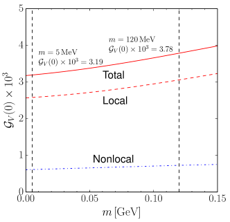
(a)

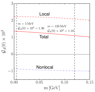
(b)

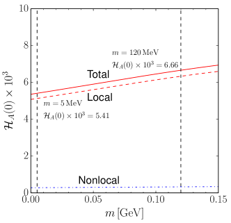
(c)

Fig. 2: Numerical results of $\mathcal{G}_{V}(0)$, $\mathcal{G}_{A}(0)$, and $\mathcal{H}_{A}(0)$ multiplied by $10^{3}$ as functions of the current quark mass $m$, which are drawn respectively in the left, middle, and right panels. The dotted and dot-dashed lines depict the local and nonlocal contributions, respectively. The solid line represents the total contribution.

Figure 2 draws the numerical results of $\mathcal{G}_{V}(0)$, $\mathcal{G}_{A}(0)$, and $\mathcal{H}_{A}(0)$ as functions of a current quark mass $m$ in the range between $m=5$ MeV and $m=120$ MeV, in which the effects of flavor SU(3) symmetry breaking are clearly exhibited. In the case of $\mathcal{G}_{V}$, the local contribution increases monotonically as the value of $m$ grows. The magnitude of the nonlocal part gets only slightly larger when $m$ increases. Hence, the $m$ dependence is governed by the local terms. $\mathcal{H}_{A}$ depicted in the right panel of Fig. 2 shows a similar tendency to $\mathcal{G}_{V}$. On the other hand, $\mathcal{G}_{A}$ decreases as $m$ increases. As displayed in Fig. 2, the effects of the SU(3) symmetry breaking increase the vector form factor $F_{V}(0)$ and the second axial-vector form factor $R_{A}(0)$ for the radiative kaon decay by about $16~{}\%$ and $19~{}\%$, compared to the corresponding pion form factors. On the other hand, they lessen the axial-vector form factor $F_{A}(0)$ for the radiative kaon decay in comparison with the corresponding pion axial-vector form factor. These kinds of tendencies of $\mathcal{G}_{V}(0)$, $\mathcal{G}_{A}(0)$, and $\mathcal{H}_{A}(0)$ determine the pion and kaon weak form factors at $Q^{2}=0$ with corresponding current quark masses, $m=5$ MeV and $m=120$ MeV.

Table 1: Results of the form factors at $Q^{2}=0$ and slope parameters in comparison with those from $\chi$PT to order $\mathcal{O}(p^{6})$ and the experimental data. The results listed in the column denoted by “D.P.” are obtained by using the original momentum-dependent quark mass (15) derived in Ref. Diakonov:1985eg , whereas those in the last column designated by “Dipole” are obtained by using the dipole-type form factor given in Eq. (16).

	CHPT$p^{6}$ Geng:2003mt	Experimental data			Present results
		$K\to e(\mu)\nu e^{+}e^{-}$ Poblaguev:2002ug	$K\to e\nu\gamma$	$K\to\mu\nu\gamma$	D.P.	Dipole
$F_{V}(0)$	0.078(5)	0.112(28)			0.118	0.114
$F_{A}(0)$	0.034	0.035(30)			0.027	0.033
$R_{A}(0)$		0.227(32)			0.201	0.200
$F_{V}(0)+F_{A}(0)$	0.112(5)	0.147(40)	0.125(8) Ambrosino:2009aa	0.165(18) Adler:2000vk	0.145	0.147
$F_{V}(0)-F_{A}(0)$	0.044(5)	0.077(45)		0.21(8)Duk:2010bs , 0.126(74)Tchikilev:2010wy	0.092	0.081
$R_{A}(0)+F_{V}(0)$		0.338(45)			0.319	0.314
$R_{A}(0)-F_{V}(0)$		0.114(42)			0.083	0.086
$R_{A}(0)+F_{A}(0)$		0.262(21)			0.228	0.233
$R_{A}(0)-F_{A}(0)$		0.191(61)			0.174	0.167
$a_{V}$	0.3(1)		0.38(4) Ambrosino:2009aa		0.404	0.379
$a_{A}$					0.159	0.192

In Table 1, we list the results of the form factors at $Q^{2}=0$, various combinations of them, and slope parameters $a_{V}$ and $a_{A}$ in comparison with those from $\chi$PT to order $\mathcal{O}(p^{6})$ and the experimental data. The slope parameters are defined from the following parametrizations of the vector and axial-vector form factors for the radiative kaon decay

$$F_{V}(Q^{2})=\frac{F_{V}(0)}{1+a_{V}\frac{Q^{2}}{m_{K}^{2}}},\;\;\;F_{A}(Q^{2})=\frac{F_{A}(0)}{1+a_{A}\frac{Q^{2}}{m_{K}^{2}}},$$ (46)

where $a_{V}$ and $a_{A}$ denote the slope parameters for the vector and axial-vector form factors, respectively. The results listed in the column denoted by “D.P.” are obtained by using the original momentum-dependent quark mass defined in Eq. (15) Diakonov:1985eg , whereas those in the last column designated by “Dipole” are produced by employing the dipole-type form factor given in Eq. (16). The results with the two different form factors are not much different from each other.

Generally, the present numerical results are in very good agreement with the experimental data taken from Ref. Poblaguev:2002ug , where kaon radiative decays $K^{+}\to\mu^{+}\nu e^{+}e^{-}$ and $K^{+}\to e^{+}\nu e^{+}e^{-}$ were experimentally studied. The experimental data presented in the third column of Table 1 are those from the combined fit including both radiative decays $K^{+}\to\mu^{+}\nu e^{+}e^{-}$ and $K^{+}\to e^{+}\nu e^{+}e^{-}$ Poblaguev:2002ug . Experimentally, more plausible quantities are $F_{V}(0)+F_{A}(0)$ and $F_{V}(0)-F_{A}(0)$. The experimental data indicate consistently that the decay $K\to\mu\nu\gamma$ yields the larger values of $F_{V}+F_{A}$ than the electron channel $K\to e\nu\gamma$. For example, Ref. Poblaguev:2002ug reported the mean value of $F_{V}+F_{A}=0.155$ from the $K^{+}\to\mu^{+}\nu e^{+}e^{-}$ data whereas $F_{V}+F_{A}=0.125$ from the $K^{+}\to e^{+}\nu e^{+}e^{-}$ data and the weighted average value is in TABLE 1. The results of $F_{V}-F_{A}$ show similar tendencies. The comparison of the KLOE data Ambrosino:2009aa with those of the E787 Experiment Adler:2000vk leads to the same conclusion. The data on $K^{-}\to\mu^{-}\nu\gamma$ from the ISTRA+ Collaboration Duk:2010bs gives a rather large value of $F_{V}-F_{A}$, i.e. $F_{V}-F_{A}=0.21$ that is almost three times larger than that from Ref. Poblaguev:2002ug . Another analysis from the ISTRA+ Collaboration yields $F_{V}-F_{A}=0.126$ with the exotic tensor interaction excluded Tchikilev:2010wy . The present results lie between those from the $\mu$ and electron channels. In general, the results from $\mathcal{O}(p^{6})$ $\chi$PT are underestimated, compared with the present ones except for $F_{A}$ of which the value is almost the same as our result. The vector slope parameter $a_{V}$ is experimentally known to be $a_{V}=0.38(4)$ from Ref. Ambrosino:2009aa where as $a_{A}$ is still at large experimentally. The present results of $a_{V}$ are $0.404$ and $0.379$, which are in good agreement with the KLOE data. We predict $a_{A}=0.159$ (D.P.) and $a_{A}=0.192$ (Dipole).

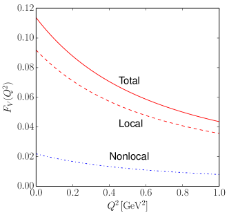
(a)

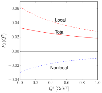
(b)

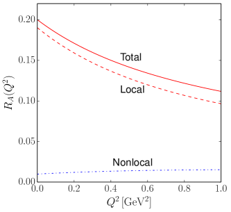
(c)

Fig. 3: Numerical results of the vector and axial-vector form factors for the radiative kaon decays as functions of $Q^{2}$. The dashed and dot-dashed curves depict respectively the local and nonlocal contributions, whereas the solid draws the total result.

In Fig. 3 we show the numerical results of the vector and axial-vector form factors of the kaon radiative decays. All these three form factors fall off monotonically as $Q^{2}$ increases. In fact, the results of the form factors for the radiative kaon decays show the same tendency as those for the radiative pion decays Shim:2017wcq , since the expressions of the form factors are the same as those for the pion decays except for the strange current quark mass, as already discussed in Fig. 2. Nevertheless let us recapitulate briefly what we have found. The nonlocal terms appear from the gauged E$\chi$A that was constructed in such a way that the relevant gauge invariance is preserved. In the left panel of Fig. 3, we find that the nonlocal contribution enhances the vector form factor by almost about 20 %. On the other hand, the nonlocal terms reduce the axial-vector form factors almost by 50 %. It implies that it is essential to preserve the gauge invariance not only theoretically but also quantitatively. The large suppression of $F_{A}(Q^{2})$ comes mainly from the nonlocal contributions that are related to diagrams (b)-(e) in Fig. 1. The contributions from them have been considered not only by two of the present authors in the same model Shim:2017wcq but also by D. G. Dumm et al. in a nonlocal NJL model Dumm:2010hh ; GomezDumm:2012qh for the radiative pion decay. We want to emphasize that they are also crucial to the description of $F_{A}(Q^{2})$ for the case of kaon. The nonlocal contribution turns out to be marginal to the second axial-vector form factor.

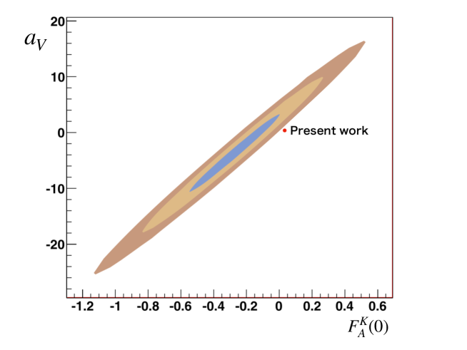
Fig. 4: Comparison with the $3\sigma$-ellipse taken from Fig. 22 of Ref. Duk:2010bs , where $F_{V}(0)$ is fixed from $\mathcal{O}(p^{6})$ $\chi$PT and $a_{V}$ and $F_{A}$ are considered as fitting parameters. The red blob denotes the present results ($a_{V}=0.383$, $F_{A}=0.033$).

Figure 4 illustrates the $3\sigma$-ellipse taken from Fig. 22 of Ref. Duk:2010bs , where $F_{V}(0)$ is fixed from $\mathcal{O}(p^{6})$ $\chi$PT and $a_{V}$ and $F_{A}$ are regarded as fitting parameters. We can put the present results $a_{V}=0.404$ and $F_{A}=0.027$ as a red blob in Fig. 4. Interestingly, the red blob turns out to be slightly higher than that of $\mathcal{O}(p^{6})$ $\chi$PT, which indicates that the present ones are closer to the $3\sigma$ boundary. However, note that the value of $F_{V}$ obtained in the present work is $0.118$ and $0.114$ as shown in Table 1, which is almost the same as the experimental data given in Ref. Poblaguev:2002ug .

Finally, we extract the parameters for the $p$-pole parametrizations of the vector and axial-vector form factors for the kaon radiative decays. In lattice QCD, the $p$-pole parametrization for a form factor is often introduced to fit various lattice data Brommel:2006ww ; Brommel:2007xd . Although there is no the results from lattice QCD yet, it will be useful to provide the parameters here so that one can easily compare the present results with those of lattice QCD in near future. The $p$-pole parametrizations of the vector and axial-vector form factors are expressed as

$$F_{V}(Q^{2})=\frac{F_{V}(0)}{\left(1+\frac{Q^{2}}{p_{V}m_{p_{V}}^{2}}\right)^{p_{V}}},\;\;\;F_{A}(Q^{2})=\frac{F_{A}(0)}{\left(1+\frac{Q^{2}}{p_{A}m_{p_{A}}^{2}}\right)^{p_{A}}},\;\;\;R_{A}(Q^{2})=\frac{R_{A}(0)}{\left(1+\frac{Q^{2}}{p_{R}m_{p_{R}}^{2}}\right)^{p_{R}}},$$ (47)

where the results of the parameters $p_{V}$, $p_{A}$, $p_{R}$, $M_{p_{A}}$, $M_{p_{A}}$, and $M_{p_{R}}$ are listed in Table 2.

Table 2: The results of the p-pole parameters. The results listed in the row denoted by “D.P.” are obtained by using the original momentum-dependent quark mass (15) derived in Ref. Diakonov:1985eg , whereas those in the last row designated by “Dipole” are obtained by using the dipole-type form factor given in Eq. (16).

	$p_{V}$	$M_{p_{V}}$	$p_{A}$	$M_{p_{A}}$	$p_{R}$	$M_{p_{R}}$
Dipole	$1.26$	$0.832$ GeV	$1.20$	$1.15$ GeV	$0.779$	$1.07$ GeV

VI Summary and conclusion

In the present work, we investigated the vector and axial-vector form factors for kaon radiative decays within the framework of the gauged nonlocal effective chiral action, which constitute the essential part of the structure-dependent decay amplitude. We scrutinized the effects of the flavor SU(3) symmetry breaking, releasing the strange current quark mass from its fixed value $m_{\mathrm{s}}=120$ MeV. The results showed how the vector and axial-vector form factors undergo changes when the current quark mass $m$ is varied. We found that the vector form factor and the second axial-vector form factor increase monotonically as $m$ increases. On the other hand, the axial-vector form factor lessens as $m$ increases.

The numerical results of the form factors are in good agreement with the experimental data. In general, the experimental data extracted from the radiative decay of the kaon to the electron are smaller than those from the radiative pion decay to the muon. The present results are found to lie between the data taken from the electron and muon channels. The slope parameter for the axial-vector form factor was predicted. The $Q^{2}$ dependences of all the three form factors were presented and the general tendency is almost the same as in the case of pion radiative decay. The nonlocal contributions enhance the vector form factor while they reduce the axial-vector one. However, their effects are marginal on the second axial-vector form factors. We compared the present results of the vector slope parameter and the axial-vector form factor with the $3\sigma$-ellipse taken from the ISTRA+ Collaboration. Finally, we provided the parameters for the $p$-pole parametrization of the vector and axial-vector form factors.

In the present work, we concentrated only on the vector and axial-vector form factors for kaon radiative decays. However, it is of great importance to consider the tensor form factors, though they must be small experimentally. Since the nonlocal chiral quark model from the instanton vacuum is a well-defined theoretical framework and furthermore it does not have any additional free parameter to handle, it is very interesting to consider the tensor form factors for the kaon radiative decay. There are at least two important physical implications on them. Firstly, it offers a possible new physics beyond the standard model, in particular, related to dark photons. Secondly, the transition tensor form factors allow one to examine the spin structure of the kaon in the course of its radiative decay. The relevant works are under way.

References

- (1) V. G. Vaks and B. L. Ioffe, Nuovo Cim. 10 (1958) 342.
- (2) S. A. Bludman and J. A. Young, Phys. Rev. 118 (1960) 602.
- (3) D. A. Bryman, P. Depommier and C. Leroy, Phys. Rept. 88 (1982) 151.
- (4) D. E. Neville, Phys. Rev. 124 (1961) 2037.
- (5) A. Kanazawa, M. Sugawara, and K. Tanaka, Phys. Rev. 122 (1961) 341.
- (6) V. Cirigliano, G. Ecker, H. Neufeld, A. Pich and J. Portoles, Rev. Mod. Phys. 84 (2012) 399. [arXiv:1107.6001 [hep-ph]].
- (7) M. Tanabashi et al. (Particle Data Group), Phys. Rev. D 98 (2018) 030001.
- (8) K. S. Heard et al., Phys. Lett. 55B (1975) 324.
- (9) J. Heintze et al., Phys. Lett. 60B (1976) 302.
- (10) J. Heintze et al., Nucl. Phys. B 149 (1979) 365.
- (11) Y. Akiba et al., Phys. Rev. D 32 (1985) 2911.
- (12) V. V. Barmin et al., Sov. J. Nucl. Phys. 47 (1988) 643 [Yad. Fiz. 47 (1988) 1011].
- (13) V. S. Demidov, V. A. Dobrokhotov, E. A. Lyublev and A. N. Nikitenko, Sov. J. Nucl. Phys. 52 (1990) 1006 [Yad. Fiz. 52 (1990) 1595].
- (14) S. Adler et al. [E787 Collaboration], Phys. Rev. Lett. 85 (2000) 2256 [hep-ex/0003019].
- (15) A. A. Poblaguev et al., Phys. Rev. Lett. 89 (2002) 2256 [hep-ex/0204006].
- (16) F. Ambrosino et al. [KLOE Collaboration], Eur. Phys. J. C 64 (2009) 627 Erratum: [Eur. Phys. J. 65 (2010) 703] [arXiv:0907.3594 [hep-ex]].
- (17) V. A. Duk et al. [ISTRA+ Collaboration], Phys. Lett. B 695 (2011) 59 [arXiv:1005.3517 [hep-ex]].
- (18) O. Tchikilev et al., [arXiv:1001.0374 [hep-ex]].
- (19) J. Gasser and H. Leutwyler, Nucl. Phys. B 250 (1985) 465.
- (20) J. F. Donoghue and B. R. Holstein, Phys. Rev. D 40 (1989) 3700.
- (21) J. Bijnens, G. Ecker and J. Gasser, In *Maiani, L. (ed.) et al.: The DAPHNE physics handbook, vol. 1* 115-190 and Frascati INFN - LNF-92-047(P) (92/06,rec.Nov.) 88 p. (see Book Index) [hep-ph/9208204].
- (22) J. Bijnens, G. Ecker and J. Gasser, Nucl. Phys. B 396 (1993) 81 [hep-ph/9209261].
- (23) C. Q. Geng, I. L. Ho and T. H. Wu, Nucl. Phys. B 684 (2004) 281 [hep-ph/0306165]
- (24) C. H. Chen, C. Q. Geng and C. C. Lih, Phys. Rev. D 77 (2008) 014004
- (25) C. E. Carlson and B. C. Rislow, Phys. Rev. D 89 (2014) 035003 [arXiv:1310.2786 [hep-ph]].
- (26) M. Fabbrichesi, E. Gabrielli and B. Mele, Phys. Rev. Lett. 119 (2017) 031801 [arXiv:1705.03470 [hep-ph]].
- (27) D. Diakonov and V. Y. Petrov, Nucl. Phys. B 272 (1986) 457.
- (28) D. Diakonov, Prog. Part. Nucl. Phys. 51 (2003) 173 [hep-ph/0212026].
- (29) M. M. Musakhanov and H.-Ch. Kim, Phys. Lett. B 572 (2003) 181 [hep-ph/0206233].
- (30) H.-Ch. Kim, M. Musakhanov and M. Siddikov, Phys. Lett. B 608 (2005) 95 [hep-ph/0411181].
- (31) H.-Ch. Kim, M. M. Musakhanov and M. Siddikov, Phys. Lett. B 633 (2006) 701 [hep-ph/0508211].
- (32) K. Goeke, H.-Ch. Kim, M. M. Musakhanov and M. Siddikov, Phys. Rev. D 76 (2007) 116007 [arXiv:0708.3526 [hep-ph]].
- (33) K. Goeke, M. M. Musakhanov and M. Siddikov, Phys. Rev. D 76 (2007) 076007 [arXiv:0707.1997 [hep-ph]].
- (34) E. V. Shuryak, Nucl. Phys. B 203 (1982) 93.
- (35) T. Schäfer and E. V. Shuryak, Rev. Mod. Phys. 70 (1998) 323 [hep-ph/9610451]
- (36) M. C. Chu, J. M. Grandy, S. Huang and J. W. Negele, Phys. Rev. D 49 (1994) 6039 [hep-lat/9312071].
- (37) J. W. Negele, Nucl. Phys. Proc. Suppl. 73 (1999) 92 [hep-lat/9810053].
- (38) T. A. DeGrand, Phys. Rev. D 64 (2001) 094508 [hep-lat/0106001].
- (39) M. Cristoforetti, P. Faccioli, M. C. Traini and J. W. Negele, Phys. Rev. D 75 (2007) 034008 [hep-ph/0605256].
- (40) M. Musakhanov, Eur. Phys. J. C 9 (1999) 235 [hep-ph/9810295].
- (41) M. Musakhanov, hep-ph/0104163.
- (42) M. Musakhanov, Nucl. Phys. A 699 (2002) 340.
- (43) S. i. Nam and H.-Ch. Kim, Phys. Lett. B 647 (2007) 145 [hep-ph/0605041].
- (44) M. Chretien and R. E. Peierls, Proc. Roy. Soc. Lond. A 223 (1954) 468.
- (45) P. V. Pobylitsa, Phys. Lett. B 226 (1989) 387.
- (46) R. D. Bowler and M. C. Birse, Nucl. Phys. A 582 (1995) 655 [hep-ph/9407336].
- (47) M. M. Musakhanov and F. C. Khanna, hep-ph/9605232.
- (48) S. i. Nam and H.-Ch. Kim, Phys. Rev. D 77 (2008) 094014 [arXiv:0709.1745 [hep-ph]].
- (49) S. i. Nam and H.-Ch. Kim, Phys. Rev. D 75 (2007) 094011 [hep-ph/0703089 [HEP-PH]].
- (50) S. i. Nam and H.-Ch. Kim, Phys. Rev. D 74 (2006) 076005 [hep-ph/0609267].
- (51) S.-I. Shim and H.-Ch. Kim, Phys. Lett. B 772 (2017) 687 [arXiv:1704.03263 [hep-ph]].
- (52) D. Gomez Dumm, S. Noguera and N. N. Scoccola, Phys. Lett. B 698 (2011) 236 [arXiv:1011.6403 [hep-ph]]
- (53) D. Gomez Dumm, S. Noguera and N. N. Scoccola, Phys. Rev. D 86 (2012) 074020 [arXiv:1205.2730 [hep-ph]]
- (54) D. Brommel et al. [QCDSF/UKQCD Collaboration], Eur. Phys. J. C 51 (2007) 335 [hep-lat/0608021].
- (55) D. Brommel et al. [QCDSF and UKQCD Collaborations], Phys. Rev. Lett. 101 (2008) 122001 [arXiv:0708.2249 [hep-lat]].