High-order Solution Transfer between Curved Triangular Meshes

Abstract.

The problem of solution transfer between meshes arises frequently in computational physics, e.g. in Lagrangian methods where remeshing occurs. The interpolation process must be conservative, i.e. it must conserve physical properties, such as mass. We extend previous works — which described the solution transfer process for straight sided unstructured meshes — by considering high-order isoparametric meshes with curved elements. To facilitate solution transfer, we numerically integrate the product of shape functions via Green’s theorem along the boundary of the intersection of two curved elements. We perform a numerical experiment and confirm the expected accuracy by transferring test fields across two families of meshes.

Keywords: Remapping, Curved Meshes, Lagrangian, Solution Transfer, Discontinuous Galerkin

1. Introduction

Solution transfer between meshes is a common problem that has practical applications to many methods in computational physics. For example, by allowing the underyling computational domain to change during a simulation, computational effort can be focused dynamically to resolve sensitive features of a numerical solution. Mesh adaptivity, this in-flight change in the mesh, requires translating the numerical solution from the old mesh to the new, i.e. solution transfer. As another example, Lagrangian or particle-based methods treat each node in the mesh as a particle and so with each timestep the mesh travels with the fluid. However, over (typically limited) time the mesh becomes distorted and suffers a loss in element quality which causes catastrophic loss in the accuracy of computation. To overcome this, the domain must be remeshed or rezoned and the solution must be transferred (remapped) onto the new mesh configuration. A few scenarios where solution transfer is necessary will be considered below to motivate the “black box” solution transfer algorithm.

Solution transfer is needed when a solution (approximated by a discrete field) is known on a donor mesh and must be transferred to a target mesh. In many applications, the field must be conserved for physical reasons, e.g. mass or energy cannot leave or enter the system, hence the focus on conservative solution transfer (typically using Galerkin or $L_{2}$-minimizing methods).

When pointwise interpolation is used to transfer a solution, quantities with physical meaning (e.g. mass, concentration, energy) may not be conserved. To address this, there have been many explorations of conservative interpolation. Since solution transfer is so commonly needed in physical applications, this problem of conservative interpolation has been considered already for straight sided meshes. However, both to allow for greater geometric flexibility and for high order of convergence, this paper will consider the case of curved isoparametric meshes. High-order methods have the ability to produce highly accurate solutions with low dissipation and low dispersion error, however, they typically require curved meshes. In addition, curved elements have advantages in problems that involve geometries that change over time, such as flapping flight or fluid-structure interactions.

The common refinement approach in [JH04] is used to compare several methods for solution transfer across two meshes. However, the problem of constructing a common refinement is not discussed there. The problem of constructing such a refinement is considered in [FPP⁺09, FM11] (called a supermesh by the authors). However, the solution transfer becomes considerably more challenging for curved meshes. For a sense of the difference between the straight sided and curved cases, consider the problem of intersecting an element from the donor mesh with an element from the target mesh. If the elements are triangles, the intersection is either a convex polygon or has measure zero. If the elements are curved, the intersection can be non-convex and can even split into multiple disjoint regions. In [CGQ18], a related problem is considered where squares are allowed to curve along characteristics and the solution is remapped onto a regular square grid.

Lagrangian methods treat each point in the physical domain as a “particle” which moves along a characteristic curve over time and then monitor values associated with the particle (heat / energy, velocity, pressure, density, concentration, etc.). They are an effective way to solve PDEs, even with higher order or non-linear terms [DKR12]. This approach transforms the numerical solution of PDEs into a family of numerical solutions to many independent ODEs. It allows the use of familiar and well understood ODE solvers. In addition, Lagrangian methods often have less restrictive conditions on time steps than Eulerian methods. When solving PDEs on unstructured meshes with Lagrangian methods, the nodes move (since they are treated like particles) and the mesh “travels”. A flow-based change to a mesh can cause problems if it causes the mesh to leave the domain being analyzed or if it distorts the mesh until the element quality is too low in some mesh elements. Over enough time, the mesh can even tangle (i.e. elements begin to overlap).

To deal with distortion, one can allow the mesh to adapt in between time steps. In addition to improving mesh quality, mesh adaptivity can be used to dynamically focus computational effort to resolve sensitive features of a numerical solution. From [IK04]

In order to balance the method’s approximation quality and its computational costs effectively, adaptivity is an essential requirement, especially when modelling multiscale phenomena.

For more on mesh adaptivity, see [BR78, PVMZ87, PUdOG01].

In either case, the change in the mesh between time steps requires transferring a known solution on the discarded mesh to the mesh produced by the remeshing process. Without the ability to change the mesh, Lagrangian methods (or, more generally, ALE [HAC74]) would not be useful, since after a limited time the mesh will distort.

To allow for greater geometric flexibility and for high order of convergence, curved mesh elements can be used in the finite element method. Though the complexity of a method can steeply rise when allowing curved elements, the trade for high-order convergence can be worth it. (See [WFA⁺13] for more on high-order CFD methods.) Curved meshes can typically represent a given geometry with far fewer elements than a straight sided mesh. The increase in accuracy also allows for the use of fewer elements, which in turn can also facilitate a reduction in the overall computation time.

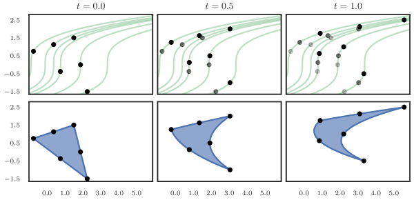
Figure 1.1. Movement of nodes in a quadratic element under distortion caused by particle motion along the velocity field $\left[y^{2}\;1\right]^{T}$ from $t=0$ to $t=1$ with $\Delta t=1/2$. The green curves represent the characteristics that each node travels along.

Even if the domain has no inherent curvature, high-order (degree $p$) shape functions allow for order $p+1$ convergence, which is desirable in it’s own right. However, even in such cases, a Lagrangian method must either curve the mesh or information about the flow of the geometry will be lost. Figure 1.1 shows what happens to a given quadratic element as the nodes move along the characteristics given by the velocity field $\left[\begin{array}[]{c c}y^{2}&1\end{array}\right]^{T}$. This element uses the triangle vertices and edge midpoints to determine the shape functions. However, as the nodes move with the flow, the midpoints are no longer on the lines connecting the vertex nodes. To allow the mesh to more accurately represent the solution, the edges can instead curve so that the midpoint nodes remain halfway between (i.e. half of the parameter space) the vertex nodes along an edge.

In multiphysics simulations, a problem is partitioned into physical components. This partitioning can apply to both the physical domain (e.g. separating a solid and fluid at an interface) and the simulation solution itself (e.g. solving for pressure on one mesh and velocity on another). Each (multi)physics component is solved for on its own mesh. When the components interact, the simulation solution must be transferred between those meshes.

In a similar category of application, solution transfer enables the comparison of solutions defined on different meshes. For example, if a reference solution is known on a very fine special-purpose mesh, the error can be computed for a coarse mesh by transferring the solution from the fine mesh and taking the difference. Or, if the same method is used on different meshes of the same domain, the resulting computed solutions can be compared via solution transfer. Or, if two different methods use two different meshes of the same domain.

Conservative solution transfer has been around since the advent of ALE, and as a result much of the existing literature focuses on mesh-mesh pairs that will occur during an ALE-based simulation. When flow-based mesh distortion occurs, elements are typically “flipped” (e.g. a diagonal is switched in a pair of elements) or elements are subdivided or combined. These operations are inherently local, hence the solution transfer can be done locally across known neighbors. Typically, this locality is crucial to solution transfer methods. In [MS03], the transfer is based on partitioning elements of the updated mesh into components of elements from the old mesh and “swept regions” from neighbouring elements. In [KS08], the (locally) changing connectivity of the mesh is addressed. In [GKS07], the local transfer is done on polyhedral meshes.

Global solution transfer instead seeks to conserve the solution across the whole mesh. It makes no assumptions about the relationship between the donor and target meshes. The loss in local information makes the mesh intersection problem more computationally expensive, but the added flexibility reduces timestep restrictions since it allows remeshing to be done less often. In [Duk84, DK87], a global transfer is enabled by transforming volume integrals to surface integrals via the divergence theorem to reduce the complexity of the problem.

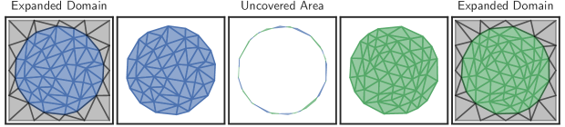
Figure 1.2. Partially overlapping meshes on a near identical domain. Both are linear meshes that approximate the unit disc in $\mathbf{R}^{2}$. The outermost columns show how the domain of each mesh can be expanded so they agree.

In this paper, an algorithm for conservative solution transfer between curved meshes will be described. This method applies to meshes in $\mathbf{R}^{2}$. Application to meshes in $\mathbf{R}^{3}$ is a direction for future research, though the geometric kernels (see Chapter A) become significantly more challenging to describe and implement. In addition, the method will assume that every element in the target mesh is contained in the donor mesh. This ensures that the solution transfer is interpolation. In the case where all target elements are partially covered, extrapolation could be used to extend a solution outside the domain, but for totally uncovered elements there is no clear correspondence to elements in the donor mesh.

The case of partially overlapping meshes can be addressed in particular cases (i.e. with more information). For example, consider a problem defined on $\Omega=\mathbf{R}^{2}$ and solution that tends towards zero as points tend to infinity. A typical approach may be to compute the solution on a circle of large enough radius and consider the numerical solution to be zero outside the circle. Figure 1.2 shows how solution transfer could be performed in such cases when the meshes partially overlap: construct a simple region containing both computational domains and then mesh the newly introduced area. However, the assumption that the numerical solution is zero in the newly introduced area is very specific and a similar approach may not apply in other cases of partial overlap.

Some attempts ([Ber87, CH94, CDS99]) have been made to interpolate fluxes between overlapping meshes. These perform an interpolation on the region common to both meshes and then numerically solve the PDE to determine the values on the uncovered elements.

When solving some PDEs with viscoelastic fields, additional nodes must be tracked at quadrature points. As the mesh travels, these quadrature points must be moved as well in a way that is consistent with the standard nodes that define the element. The solution transfer method described here does not provide a way either to determine quadrature points on a target mesh or to map the field onto known quadrature points.

This paper is organized as follows. Section 2 establishes common notation and reviews basic results relevant to the topics at hand. Section A is an in-depth discussion of the computational geometry methods needed to implement to enable solution transfer. Section 3 (and following) describes the solution transfer process and gives results of some numerical experiments confirming the rate of convergence.

2. Preliminaries

2.1. General Notation

We’ll refer to $\mathbf{R}$ for the reals, $\mathcal{U}$ represents the unit triangle (or unit simplex) in $\mathbf{R}^{2}$:

$$\mathcal{U}=\left\{(s,t)\mid 0\leq s,t,s+t\leq 1\right\}.$$ (2.1)

When dealing with sequences with multiple indices, e.g. $s_{m,n}=m+n$, we’ll use bold symbols to represent a multi-index: $\bm{i}=(m,n)$. The binomial coefficient $\binom{n}{k}$ is equal to $\frac{n!}{k!(n-k)!}$ and the trinomial coefficient $\binom{n}{i,j,k}$ is equal to $\frac{n!}{i!j!k!}$ (where $i+j+k=n$). The notation $\delta_{ij}$ represents the Kronecker delta, a value which is $1$ when $i=j$ and $0$ otherwise.

2.2. Bézier Curves

A Bézier curve is a mapping from the unit interval that is determined by a set of control points $\left\{\bm{p}_{j}\right\}_{j=0}^{n}\subset\mathbf{R}^{d}$. For a parameter $s\in\left[0,1\right]$, there is a corresponding point on the curve:

$$b(s)=\sum_{j=0}^{n}\binom{n}{j}(1-s)^{n-j}s^{j}\bm{p}_{j}\in\mathbf{R}^{d}.$$ (2.2)

This is a combination of the control points weighted by each Bernstein basis function $B_{j,n}(s)=\binom{n}{j}(1-s)^{n-j}s^{j}$. Due to the binomial expansion $1=(s+(1-s))^{n}=\sum_{j=0}^{n}B_{j,n}(s)$, a Bernstein basis function is in $\left[0,1\right]$ when $s$ is as well. Due to this fact, the curve must be contained in the convex hull of it’s control points.

2.3. Bézier Triangles

A Bézier triangle ([Far01, Chapter 17]) is a mapping from the unit triangle $\mathcal{U}$ and is determined by a control net $\left\{\bm{p}_{i,j,k}\right\}_{i+j+k=n}\subset\mathbf{R}^{d}$. A Bézier triangle is a particular kind of Bézier surface, i.e. one in which there are two cartesian or three barycentric input parameters. Often the term Bézier surface is used to refer to a tensor product or rectangular patch. For $(s,t)\in\mathcal{U}$ we can define barycentric weights $\lambda_{1}=1-s-t,\lambda_{2}=s,\lambda_{3}=t$ so that

$$1=\left(\lambda_{1}+\lambda_{2}+\lambda_{3}\right)^{n}=\sum_{\begin{subarray}{c}i+j+k=n\\ i,j,k\geq 0\end{subarray}}\binom{n}{i,j,k}\lambda_{1}^{i}\lambda_{2}^{j}\lambda_{3}^{k}.$$ (2.3)

Using this we can similarly define a (triangular) Bernstein basis

$$B_{i,j,k}(s,t)=\binom{n}{i,j,k}(1-s-t)^{i}s^{j}t^{k}=\binom{n}{i,j,k}\lambda_{1}^{i}\lambda_{2}^{j}\lambda_{3}^{k}$$ (2.4)

that is in $\left[0,1\right]$ when $(s,t)$ is in $\mathcal{U}$. Using this, we define points on the Bézier triangle as a convex combination of the control net:

$$b(s,t)=\sum_{i+j+k=n}\binom{n}{i,j,k}\lambda_{1}^{i}\lambda_{2}^{j}\lambda_{3}^{k}\bm{p}_{i,j,k}\in\mathbf{R}^{d}.$$ (2.5)

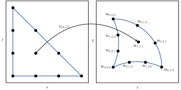
Figure 2.1. Cubic Bézier triangle

Rather than defining a Bézier triangle by the control net, it can also be uniquely determined by the image of a standard lattice of points in $\mathcal{U}$: $b\left(j/n,k/n\right)=\bm{n}_{i,j,k}$; we’ll refer to these as standard nodes. Figure 2.1 shows these standard nodes for a cubic triangle in $\mathbf{R}^{2}$. To see the correspondence, when $p=1$ the standard nodes are the control net

$$b(s,t)=\lambda_{1}\bm{n}_{1,0,0}+\lambda_{2}\bm{n}_{0,1,0}+\lambda_{3}\bm{n}_{0,0,1}$$ (2.6)

and when $p=2$

$$b(s,t)=\lambda_{1}\left(2\lambda_{1}-1\right)\bm{n}_{2,0,0}+\lambda_{2}\left(2\lambda_{2}-1\right)\bm{n}_{0,2,0}+\lambda_{3}\left(2\lambda_{3}-1\right)\bm{n}_{0,0,2}+\\ 4\lambda_{1}\lambda_{2}\bm{n}_{1,1,0}+4\lambda_{2}\lambda_{3}\bm{n}_{0,1,1}+4\lambda_{3}\lambda_{1}\bm{n}_{1,0,1}.$$ (2.7)

However, it’s worth noting that the transformation between the control net and the standard nodes has condition number that grows exponentially with $n$ (see [Far91], which is related but does not directly show this). This may make working with higher degree triangles prohibitively unstable.

A valid Bézier triangle is one which is diffeomorphic to $\mathcal{U}$, i.e. $b(s,t)$ is bijective and has an everywhere invertible Jacobian. We must also have the orientation preserved, i.e. the Jacobian must have positive determinant. For example, in Figure 2.2, the image of $\mathcal{U}$ under the map $b(s,t)=\left[\begin{array}[]{c c}(1-s-t)^{2}+s^{2}&s^{2}+t^{2}\end{array}\right]^{T}$ is not valid because the Jacobian is zero along the curve $s^{2}-st-t^{2}-s+t=0$ (the dashed line). Elements that are not valid are called inverted because they have regions with “negative area”. For the example, the image $b\left(\mathcal{U}\right)$ leaves the boundary determined by the edge curves: $b(r,0)$, $b(1-r,r)$ and $b(0,1-r)$ when $r\in\left[0,1\right]$. This region outside the boundary is traced twice, once with a positive Jacobian and once with a negative Jacobian.

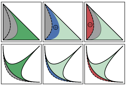
Figure 2.2. The Bézier triangle given by $b(s,t)=\left[(1-s-t)^{2}+s^{2}\;\;s^{2}+t^{2}\right]^{T}$ produces an inverted element. It traces the same region twice, once with a positive Jacobian (the middle column) and once with a negative Jacobian (the right column).

2.4. Curved Elements

We define a curved mesh element $\mathcal{T}$ of degree $p$ to be a Bézier triangle in $\mathbf{R}^{2}$ of the same degree. We refer to the component functions of $b(s,t)$ (the map that gives $\mathcal{T}=b\left(\mathcal{U}\right)$) as $x(s,t)$ and $y(s,t)$.

This fits a typical definition ([JM09, Chapter 12]) of a curved element, but gives a special meaning to the mapping from the reference triangle. Interpreting elements as Bézier triangles has been used for Lagrangian methods where mesh adaptivity is needed (e.g. [CMOP04]). Typically curved elements only have one curved side ([MM72]) since they are used to resolve geometric features of a boundary. See also [Zlá73, Zlá74]. Bézier curves and triangles have a number of mathematical properties (e.g. the convex hull property) that lead to elegant geometric descriptions and algorithms.

Note that a Bézier triangle can be determined from many different sources of data (for example the control net or the standard nodes). The choice of this data may be changed to suit the underlying physical problem without changing the actual mapping. Conversely, the data can be fixed (e.g. as the control net) to avoid costly basis conversion; once fixed, the equations of motion and other PDE terms can be recast relative to the new basis (for an example, see [PBP09], where the domain varies with time but the problem is reduced to solving a transformed conservation law in a fixed reference configuration).

2.5. Shape Functions

When defining shape functions (i.e. a basis with geometric meaning) on a curved element there are (at least) two choices. When the degree of the shape functions is the same as the degree of the function being represented on the Bézier triangle, we say the element $\mathcal{T}$ is isoparametric. For the multi-index $\bm{i}=(i,j,k)$, we define $\bm{u}_{\bm{i}}=\left(j/n,k/n\right)$ and the corresponding standard node $\bm{n}_{\bm{i}}=b\left(\bm{u}_{\bm{i}}\right)$. Given these points, two choices for shape functions present themselves:

• Pre-Image Basis: $\phi_{\bm{j}}\left(\bm{n}_{\bm{i}}\right)=\widehat{\phi}_{\bm{j}}\left(\bm{u}_{\bm{i}}\right)=\widehat{\phi}_{\bm{j}}\left(b^{-1}\left(\bm{n}_{\bm{i}}\right)\right)$ where $\widehat{\phi}_{\bm{j}}$ is a canonical basis function on $\mathcal{U}$, i.e. $\widehat{\phi}_{\bm{j}}$ a degree $p$ bivariate polynomial and $\widehat{\phi}_{\bm{j}}\left(\bm{u}_{\bm{i}}\right)=\delta_{\bm{i}\bm{j}}$

• Global Coordinates Basis: $\phi_{\bm{j}}\left(\bm{n}_{\bm{i}}\right)=\delta_{\bm{i}\bm{j}}$, i.e. a canonical basis function on the standard nodes $\left\{\bm{n}_{\bm{i}}\right\}$.

For example, consider a quadratic Bézier triangle:

$$b(s,t)=\left[\begin{array}[]{c c}4(st+s+t)&4(st+t+1)\end{array}\right]^{T}$$ (2.9)

$$\Longrightarrow\left[\begin{array}[]{c c c c c c}\bm{n}_{2,0,0}&\bm{n}_{1,1,0}&\bm{n}_{0,2,0}&\bm{n}_{1,0,1}&\bm{n}_{0,1,1}&\bm{n}_{0,0,2}\end{array}\right]=\left[\begin{array}[]{c c c c c c}0&2&4&2&5&4\\ 4&4&4&6&7&8\end{array}\right].$$ (2.13)

In the Global Coordinates Basis, we have

$$\phi^{G}_{0,1,1}(x,y)=\frac{(y-4)(x-y+4)}{6}.$$ (2.14)

For the Pre-Image Basis, we need the inverse and the canonical basis

$$b^{-1}(x,y)=\left[\begin{array}[]{c c}\frac{x-y+4}{4}&\frac{y-4}{x-y+8}\end{array}\right]\quad\text{and}\quad\widehat{\phi}_{0,1,1}(s,t)=4st$$ (2.15)

and together they give

$$\phi^{P}_{0,1,1}(x,y)=\frac{(y-4)(x-y+4)}{x-y+8}.$$ (2.16)

In general $\phi_{\bm{j}}^{P}$ may not even be a rational bivariate function; due to composition with $b^{-1}$ we can only guarantee that it is algebraic (i.e. it can be defined as the zero set of polynomials with coefficients in $\mathbf{R}\left[x,y\right]$).

2.6. Curved Polygons

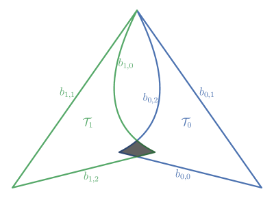
Figure 2.3. Intersection of Bézier triangles form a curved polygon.

When intersecting two curved elements, the resulting surface(s) will be defined by the boundary, alternating between edges of each element. For example, in Figure 2.3, a “curved quadrilateral” is formed when two Bézier triangles $\mathcal{T}_{0}$ and $\mathcal{T}_{1}$ are intersected.

A curved polygon is defined by a collection of Bézier curves in $\mathbf{R}^{2}$ that determine the boundary. In order to be a valid polygon, none of the boundary curves may cross, the ends of consecutive edge curves must meet and the curves must be right-hand oriented. For our example in Figure 2.3, the triangles have boundaries formed by three Bézier curves: $\partial\mathcal{T}_{0}=b_{0,0}\cup b_{0,1}\cup b_{0,2}$ and $\partial\mathcal{T}_{1}=b_{1,0}\cup b_{1,1}\cup b_{1,2}$. The intersection $\mathcal{P}$ is defined by four boundary curves: $\partial\mathcal{P}=C_{1}\cup C_{2}\cup C_{3}\cup C_{4}$. Each boundary curve is itself a Bézier curve: $C_{1}=b_{0,0}\left(\left[0,1/8\right]\right)$, $C_{2}=b_{1,2}\left(\left[7/8,1\right]\right)$, $C_{3}=b_{1,0}\left(\left[0,1/7\right]\right)$ and $C_{4}=b_{0,2}\left(\left[6/7,1\right]\right)$.

Though an intersection can be described in terms of the Bézier triangles, the structure of the control net will be lost. The region will not in general be able to be described by a mapping from a simple space like $\mathcal{U}$.

3. Galerkin Projection

3.1. Linear System for Projection

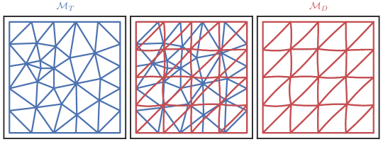
Figure 3.1. Mesh pair: donor mesh $\mathcal{M}_{D}$ and target mesh $\mathcal{M}_{T}$.

Consider a donor mesh $\mathcal{M}_{D}$ with shape function basis $\phi_{D}^{(j)}$ and a known field $\bm{q}_{D}=\sum_{j}d_{j}\phi_{D}^{(j)}$ and a target mesh $\mathcal{M}_{T}$ with shape function basis $\phi_{T}^{(j)}$ (Figure 3.1). Each shape function $\phi$ corresponds to a given isoparametric curved element (see Section 2.4) $\mathcal{T}$ in one of these meshes and has $\operatorname{supp}(\phi)=\mathcal{T}$. Additionally, the shape functions are polynomial degree $p$ (see Section 2.5 for a discussion of shape functions), but the degree of the donor mesh need not be the same as that of the target mesh. We assume that both meshes cover the same domain $\Omega\subset\mathbf{R}^{2}$, however we really only require the donor mesh to cover the target mesh.

We seek the $L_{2}$-optimal interpolant $\bm{q}_{T}=\sum_{j}t_{j}\phi_{T}^{(j)}$:

$$\left\lVert\bm{q}_{T}-\bm{q}_{D}\right\rVert_{2}=\min_{\bm{q}\in\mathcal{V}_{T}}\left\lVert\bm{q}-\bm{q}_{D}\right\rVert_{2}$$ (3.1)

where $\mathcal{V}_{T}=\operatorname{Span}_{j}\left\{\phi_{T}^{(j)}\right\}$ is the function space defined on the target mesh. Since this is optimal in the $L_{2}$ sense, by differentiating with respect to each $t_{j}$ in $\bm{q}_{T}$ we find the weak form:

$$\int_{\Omega}\bm{q}_{D}\phi_{T}^{(j)}\,dV=\int_{\Omega}\bm{q}_{T}\phi_{T}^{(j)}\,dV,\qquad\text{for all }j.$$ (3.2)

If the constant function $1$ is contained in $\mathcal{V}_{T}$, conservation follows from the weak form and linearity of the integral

$$\int_{\Omega}\bm{q}_{D}\,dV=\int_{\Omega}\bm{q}_{T}\,dV.$$ (3.3)

Expanding $\bm{q}_{D}$ and $\bm{q}_{T}$ with respect to their coefficients $\bm{d}$ and $\bm{t}$, the weak form gives rise to a linear system

$$M_{T}\bm{t}=M_{TD}\bm{d}.$$ (3.4)

Here $M_{T}$ is the mass matrix for $\mathcal{M}_{T}$ given by

$$\left(M_{T}\right)_{ij}=\int_{\Omega}\phi_{T}^{(i)}\phi_{T}^{(j)}\,dV.$$ (3.5)

In the discontinuous Galerkin case, $M_{T}$ is block diagonal with blocks that correspond to each element, so (3.4) can be solved locally on each element $\mathcal{T}$ in the target mesh. By construction, $M_{T}$ is symmetric and sparse since $\left(M_{T}\right)_{ij}$ will be $0$ unless $\phi_{T}^{(i)}$ and $\phi_{T}^{(j)}$ are supported on the same element $\mathcal{T}$. In the continuous case, $M_{T}$ is globally coupled since coefficients corresponding to boundary nodes interact with multiple elements. The matrix $M_{TD}$ is a “mixed” mass matrix between the target and donor meshes:

$$\left(M_{TD}\right)_{ij}=\int_{\Omega}\phi_{T}^{(i)}\phi_{D}^{(j)}\,dV.$$ (3.6)

Boundary conditions can be imposed on the system by fixing some coefficients, but that is equivalent to removing some of the basis functions which may in term make the projection non-conservative. This is because the removed basis functions may have been used in $1=\sum_{j}u_{j}\phi_{T}^{(j)}$.

Computing $M_{T}$ is fairly straightforward since the (bidirectional) mapping from elements $\mathcal{T}$ to basis functions $\phi_{T}^{(j)}$ supported on those elements is known. When using shape functions in the global coordinates basis (see Section 2.5), the integrand $F=\phi_{T}^{(i)}\phi_{T}^{(j)}$ will be a polynomial of degree $2p$ on $\mathbf{R}^{2}$. The domain of integration $\mathcal{T}=b\left(\mathcal{U}\right)$ is the image of a (degree $p$) map $b(s,t)$ from the unit triangle. Using substitution

$$\int_{b\left(\mathcal{U}\right)}F(x,y)\,dx\,dy=\int_{\mathcal{U}}\det(Db)F\left(x(s,t),y(s,t)\right)\,ds\,dt$$ (3.7)

(we know the map preserves orientation, i.e. $\det(Db)$ is positive). Once transformed this way, a quadrature rule on the unit triangle ([Dun85]) can be used.

On the other hand, computing $M_{TD}$ is significantly more challenging. This requires solving both a geometric problem — finding the region to integrate over — and an analytic problem — computing the integrals. The integration can be done with a quadrature rule, though finding this region is significantly more difficult.

3.2. Common Refinement

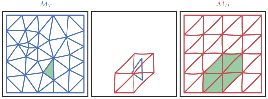
Figure 3.2. All donor elements that cover a target element

Rather than computing $M_{TD}$, the right-hand side of (3.4) can be computed directly via

$$\left(M_{TD}\bm{d}\right)_{j}=\int_{\Omega}\phi_{T}^{(j)}\bm{q}_{D}\,dV.$$ (3.8)

Any given $\phi$ is supported on an element $\mathcal{T}$ in the target mesh. Since $\bm{q}_{D}$ is piecewise defined over each element $\mathcal{T}^{\prime}$ in the donor mesh, the integral (3.8) may be problematic. In the continuous Galerkin case, $\bm{q}_{D}$ need not be differentiable across $\mathcal{T}$ and in the discontinuous Galerkin case, $\bm{q}_{D}$ need not even be continuous. This necessitates a partitioning of the domain:

$$\int_{\Omega}\phi\,\bm{q}_{D}\,dV=\int_{\mathcal{T}}\phi\,\bm{q}_{D}\,dV=\sum_{\mathcal{T}^{\prime}\in\mathcal{M}_{D}}\int_{\mathcal{T}\cap\mathcal{T}^{\prime}}\phi\left.\bm{q}_{D}\right|_{\mathcal{T}^{\prime}}\,dV.$$ (3.9)

In other words, the integral over $\mathcal{T}$ splits into integrals over intersections $\mathcal{T}\cap\mathcal{T}^{\prime}$ for all $\mathcal{T}^{\prime}$ in the donor mesh that intersect $\mathcal{T}$ (Figure 3.2). Since both $\phi$ and $\left.\bm{q}_{D}\right|_{\mathcal{T}^{\prime}}$ are polynomials on $\mathcal{T}\cap\mathcal{T}^{\prime}$, the integrals will be exact when using a quadrature scheme of an appropriate degree of accuracy. Without partitioning $\mathcal{T}$, the integrand is not a polynomial (in fact, possibly not smooth), so the quadrature cannot be exact.

In order to compute $M_{TD}\bm{d}$, we’ll need to compute the common refinement, i.e. an intermediate mesh that contains both the donor and target meshes. This will consist of all non-empty $\mathcal{T}\cap\mathcal{T}^{\prime}$ as $\mathcal{T}$ varies over elements of the target mesh and $\mathcal{T}^{\prime}$ over elements of the donor mesh. This requires solving three specific subproblems:

• Forming the region(s) of intersection between two elements that are Bézier triangles.

• Finding all pairs of elements, one each from the target and donor mesh, that intersect.

• Numerically integrating over a region of intersection between two elements.

The first subproblem is discussed in Section A.2 and the curved polygon region(s) of intersection have been described in Section 2.6. The second will be considered in Section 3.3 and the third in Section 3.4 below.

3.3. Expanding Front

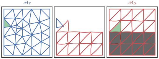
Figure 3.3. Brute force search for a donor element $\mathcal{T}^{\prime}$ that matches a fixed target element $\mathcal{T}$.

We seek to identify all pairs $\mathcal{T}$ and $\mathcal{T}^{\prime}$ of intersecting target and donor elements. The naïve approach just considers every pair of elements and takes $\mathcal{O}\left(\left|\mathcal{M}_{D}\right|\left|\mathcal{M}_{T}\right|\right)$ to complete. Taking after [FM11], we can do much better than this quadratic time search. In fact, we can compute all integrals in $\mathcal{O}\left(\left|\mathcal{M}_{D}\right|+\left|\mathcal{M}_{T}\right|\right)$. First, we fix an element of the target mesh and perform a brute-force search to find an intersecting element in the donor mesh (Figure 3.3). This has worst-case time $\mathcal{O}\left(\left|\mathcal{M}_{D}\right|\right)$.

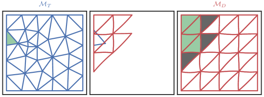
Figure 3.4. All donor elements $\mathcal{T}^{\prime}$ that cover a target element $\mathcal{T}$, with an extra layer of neighbors in the donor mesh that do not intersect $\mathcal{T}$.

Once we have such a match, we use the connectivity graph of the donor mesh to perform a breadth-first search for neighbors that also intersect the target element $\mathcal{T}$ (Figure 3.4). This search takes $\mathcal{O}\left(1\right)$ time. It’s also worthwhile to keep the first layer of donor elements that don’t intersect $\mathcal{T}$ because they are more likely to intersect the neighbors of $\mathcal{T}$. Using the list of intersected elements, a neighbor of $\mathcal{T}$ can find a donor element it intersects with in $\mathcal{O}\left(1\right)$ time (Figure 3.5). As seen, after our $\mathcal{O}\left(\left|\mathcal{M}_{D}\right|\right)$ initial brute-force search, the localized intersections for each target element $\mathcal{T}$ take $\mathcal{O}\left(1\right)$ time. So together, the process takes $\mathcal{O}\left(\left|\mathcal{M}_{D}\right|+\left|\mathcal{M}_{T}\right|\right)$.

For special cases, e.g. ALE methods, the initial brute-force search can be reduced to $\mathcal{O}\left(1\right)$. This could be enabled by tracking the remeshing process so a correspondence already exists. If a full mapping from donor to target mesh exists, the process of computing $M_{T}$ and $M_{TD}\bm{d}$ can be fully parallelized across elements of the target mesh, or even across shape functions $\phi_{T}^{(j)}$.

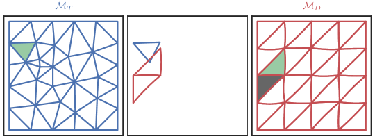
Figure 3.5. First match between a neighbor of the previously considered target element and all the donor elements that match the previously considered target element.

3.4. Integration over Curved Polygons

In order to numerically evaluate integrals of the form

$$\int_{\mathcal{T}_{0}\cap\mathcal{T}_{1}}F(x,y)\,dV$$ (3.10)

we must have a quadrature rule on these curved polygon (Section 2.6) intersections $\mathcal{T}_{0}\cap\mathcal{T}_{1}$. To do this, we transform the integral into several line integrals via Green’s theorem and then use an exact Gaussian quadrature to evaluate them. Throughout this section we’ll assume the integrand is of the form $F=\phi_{0}\phi_{1}$ where each $\phi_{j}$ is a shape function on $\mathcal{T}_{j}$. In addition, we’ll refer to the two Bézier maps that define the elements being intersected: $\mathcal{T}_{0}=b_{0}\left(\mathcal{U}\right)$ and $\mathcal{T}_{1}=b_{1}\left(\mathcal{U}\right)$.

First a discussion of a method not used. A somewhat simple approach would be be to use polygonal approximation. I.e. approximate the boundary of each Bézier triangle with line segments, intersect the resulting polygons, triangulate the intersection polygon(s) and then numerically integrate on each triangulated cell. However, this approach is prohibitively inefficient. For example, consider computing the area of $\mathcal{P}$ via an integral: $\int_{\mathcal{P}}1\,dV$. By using the actual curved boundaries of each element, this integral can be computed with relative error on the order of machine precision $\mathcal{O}\left(\mathbf{u}\right)$. On the other hand, approximating each side of $\mathcal{P}$ with $N$ line segments, the relative error is $\mathcal{O}\left(1/N^{2}\right)$. (For example, if $N=2$ an edge curve $b(s,0)$ would be replaced by segments connecting $b(0,0),b(1/2,0)$ and $b(1,0)$, i.e. $N+1$ equally spaced parameters.) This means that in order to perform as well as an exact quadrature used in the curved case, we’d need $N=\mathcal{O}\left(1/\sqrt{\mathbf{u}}\right)$.

Since polygonal approximation is prohibitively expensive, we work directly with curved edges and compute integrals on a regular domain via substitution. If two Bézier triangles intersect with positive measure, then the region of intersection is one or more disjoint curved polygons: $\mathcal{T}_{0}\cap\mathcal{T}_{1}=\mathcal{P}$ or $\mathcal{T}_{0}\cap\mathcal{T}_{1}=\mathcal{P}\cup\mathcal{P}^{\prime}\cup\cdots$. The second case can be handled in the same way as the first by handling each disjoint region independently:

$$\int_{\mathcal{T}_{0}\cap\mathcal{T}_{1}}F(x,y)\,dV=\int_{\mathcal{P}}F(x,y)\,dV+\int_{\mathcal{P}^{\prime}}F(x,y)\,dV+\cdots.$$ (3.11)

Each curved polygon $\mathcal{P}$ is defined by its boundary, a piecewise smooth parametric curve:

$$\partial\mathcal{P}=C_{1}\cup\cdots\cup C_{n}.$$ (3.12)

This can be thought of as a polygon with $n$ sides that happens to have curved edges.

Quadrature rules for straight sided polygons have been studied ([MXS09]) though they are not in wide use. Even if a polygonal quadrature rule was to be employed, a map would need to be established from a reference polygon onto the curved edges. This map could then be used with a change of coordinates to move the integral from the curved polygon to the reference polygon. The problem of extending a mapping from a boundary to an entire domain has been studied as transfinite interpolation ([Che74, GT82, Per98]), barycentric coordinates ([Wac75]) or mean value coordinates ([Flo03]). However, these maps aren’t typically suitable for numerical integration because they are either not bijective or increase the degree of the edges.

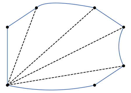
Figure 3.6. Curved polygon tessellation, done by introducing diagonals from a single vertex node.

Since simple and well established quadrature rules do exist for triangles, a valid approach would be to tessellate a curved polygon into valid Bézier triangles (Figure 3.6) and then use substitution as in (3.7). However, tessellation is challenging for both theoretical and computational reasons. Theoretical: it’s not even clear if an arbitrary curved polygon can be tessellated into Bézier triangles. Computational: the placement of diagonals and potential introduction of interior nodes is very complex in cases where the curved polygon is nonconvex. What’s more, the curved polygon is given only by the boundary, so higher degree triangles (i.e. cubic and above) introduced during tessellation would need to place interior control points without causing the triangle to invert. To get a sense for these challenges, note how the “simple” introduction of diagonals in Figure 3.7 leads to one inverted element (the gray element) and another element with area outside of the curved polygon (the yellow element). Inverted Bézier triangles are problematic because the accompanying mapping leaves the boundary established by the edge curves. For example, if the tessellation of $\mathcal{P}$ contains an inverted Bézier triangle $\mathcal{T}_{2}=b\left(\mathcal{U}\right)$ then we’ll need to numerically integrate

$$\int_{\mathcal{T}_{2}}\phi_{0}\phi_{1}\,dx\,dy=\int_{\mathcal{U}}\left|\det(Db)\right|\left(\phi_{0}\circ b\right)\left(\phi_{1}\circ b\right)\,ds\,dt.$$ (3.13)

If the shape functions are from the pre-image basis (see Section 2.5), then $\phi_{0}$ will not be defined at $b(s,t)\not\in\mathcal{T}_{0}$ (similarly for $\phi_{1}$). Additionally, the absolute value in $\left|\det(Db)\right|$ makes the integrand non-smooth since for inverted elements $\det(Db)$ takes both signs. If the shape functions are from the global coordinates basis, then tessellation can be used via an application of Theorem B.1, however this involves more computation than just applying Green’s theorem along $\partial\mathcal{P}$. By applying the theorem, inverted elements may be used in a tessellation, for example by introducing artificial diagonals from a vertex as in Figure 3.6. In the global coordinates basis, $F=\phi_{0}\phi_{1}$ can be evaluated for points in an inverted element that leave $\mathcal{T}_{0}$ or $\mathcal{T}_{1}$.

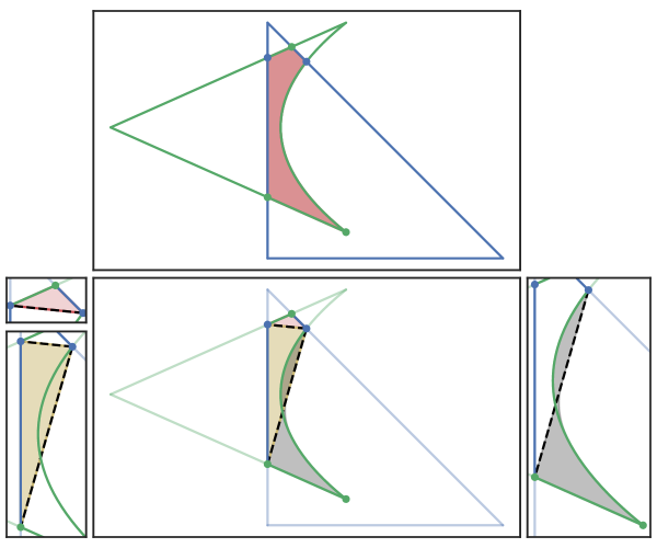
Figure 3.7. Curved polygon intersection that can’t be tessellated (with valid Bézier triangles) by introducing diagonals.

Instead, we focus on a Green’s theorem based approach. Define horizontal and vertical antiderivatives $H,V$ of the integrand $F$ such that $H_{x}=V_{y}=F$. We make these unique by imposing the extra condition that $H(0,y)\equiv V(x,0)\equiv 0$. This distinction is arbitrary, but in order to evaluate $H$ and $V$, the univariate functions $H(0,y)$ and $V(x,0)$ must be specified. Green’s theorem tells us that

$$\int_{\mathcal{P}}2F\,dV=\int_{\mathcal{P}}H_{x}+V_{y}\,dV=\oint_{\partial\mathcal{P}}H\,dy-V\,dx=\sum_{j}\int_{C_{j}}H\,dy-V\,dx.$$ (3.14)

For a given curve $C$ with components $x(r),y(r)$ defined on the unit interval, this amounts to having to integrate

$$G(r)=H(x(r),y(r))y^{\prime}(r)-V(x(r),y(r))x^{\prime}(r).$$ (3.15)

To do this, we’ll use Gaussian quadrature with degree of accuracy sufficient to cover the degree of $G(r)$.

If the shape functions are in the global coordinates basis (Section 2.5), then $G$ will also be a polynomial. This is because for these shape functions $F=\phi_{0}\phi_{1}$ will be polynomial on $\mathbf{R}^{2}$ and so will $H$ and $V$ and since each curve $C$ is a Bézier curve segment, the components are also polynomials. If the shape functions are in the pre-image basis, then $F$ won’t in general be polynomial, hence standard quadrature rules can’t be exact.

To evaluate $G$, we must also evaluate $H$ and $V$ numerically. For example, since $H(0,y)\equiv 0$, the fundamental theorem of calculus tells us that $H\left(\alpha,\beta\right)=\int_{0}^{\alpha}F\left(x,\beta\right)\,dx$. To compute this integral via Gaussian quadrature

$$H\left(\alpha,\beta\right)\approx\frac{\alpha}{2}\sum_{j}w_{j}F\left(\frac{\alpha}{2}(x_{j}+1),\beta\right)$$ (3.16)

we must be able to evaluate $F$ for points on the line $y=\beta$ for $x$ between $0$ and $\alpha$. If the shape functions are from the pre-image basis, it may not even be possible to evaluate $F$ for such points. Since $\left[\begin{array}[]{c c}\alpha&\beta\end{array}\right]^{T}$ is on the boundary of $\mathcal{P}$, without loss of generality assume it is on the boundary of $\mathcal{T}_{0}$. Thus, for some elements (e.g. if the point is on the bottom of the element), points $\left[\begin{array}[]{c c}\nu&\beta\end{array}\right]^{T}$ may not be in $\mathcal{T}_{0}$. Since $\operatorname{supp}(\phi_{0})=\mathcal{T}_{0}$, we could take $\phi_{0}(\nu,\beta)=0$, but this would make the integrand non-smooth and so the accuracy of the exact quadrature would be lost. But extending $\phi_{0}=\widehat{\phi}_{0}\circ b_{0}^{-1}$ outside of $\mathcal{T}_{0}$ may be impossible: even though $b_{0}$ is bijective on $\mathcal{U}$ it may be many-to-one elsewhere hence $b_{0}^{-1}$ can’t be reliably extended outside of $\mathcal{T}_{0}$.

Even if the shape functions are from the global coordinates basis, setting $H(0,y)\equiv 0$ may introduce quadrature points that are very far from $\mathcal{P}$. This can be somewhat addressed by using $H(m,y)\equiv 0$ for a suitably chosen $m$ (e.g. the minimum $x$-value in $\mathcal{P}$). Then we have $H\left(\alpha,\beta\right)=\int_{m}^{\alpha}F\left(x,\beta\right)\,dx$.

4. Numerical Experiments

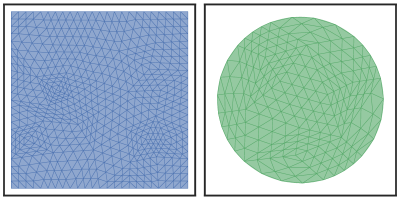
Figure 4.1. Some example meshes used during the numerical experiments; the donor meshs is on the left / blue and the target mesh is on the right / green. These meshes are the cubic approximations of each domain and have been refined twice.

A numerical experiment was performed to investigate the observed order of convergence. Three pairs of random meshes were generated, the donor on a square of width $17/8$ centered at the origin and the target on the unit disc. These domains were chosen intentionally so that the target mesh was completely covered by the donor mesh and the boundaries did not accidentally introduce ill-conditioned intersection between elements. The pairs were linear, quadratic and cubic approximations of the domains. The convergence test was done by refining each pair of meshes four times and performing solution transfer at each level. Figure 4.1 shows the cubic pair of meshes after two refinements.

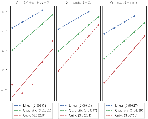
Figure 4.2. Convergence results for scalar fields on three pairs of related meshes: a linear, quadratic and cubic mesh of the same domain.

Taking after [FM11], we transfer three discrete fields in the discontinuous Galerkin (DG) basis. Each field is derived from one of the smooth scalar functions

$$\zeta_{1}(x,y) =5y^{3}+x^{2}+2y+3$$ (4.1)

$$\zeta_{2}(x,y) =\exp\left(x^{2}\right)+2y$$ (4.2)

$$\zeta_{3}(x,y) =\sin(x)+\cos(y).$$ (4.3)

For a given mesh size $h$, we expect that on a degree $p$ isoparametric mesh our solution transfer will have $\mathcal{O}\left(h^{p+1}\right)$ errors. To measure the rate of convergence:

• Choose a mesh pair $\mathcal{M}_{D}$, $\mathcal{M}_{T}$ and a known function $\zeta(x,y)$.

• Refine the meshes recursively, starting with $\mathcal{M}_{D}^{(0)}=\mathcal{M}_{D}$, $\mathcal{M}_{T}^{(0)}=\mathcal{M}_{T}$.

• Create meshes $\mathcal{M}_{D}^{(j)}$ and $\mathcal{M}_{T}^{(j)}$ from $\mathcal{M}_{D}^{(j-1)}$ and $\mathcal{M}_{T}^{(j-1)}$ by subdividing each curved element into four elements.

• Approximate $\zeta$ by a discrete field: the nodal interpolant on the donor mesh $\mathcal{M}_{D}^{(j)}$. The nodal interpolant is constructed by evaluating $\zeta$ at the nodes $\bm{n}_{j}$ corresponding to each shape function:

  $$\bm{f}_{j}=\sum_{i}\zeta\left(\bm{n}_{i}\right)\phi_{D}^{(i)}.$$ (4.4)

• Transfer $\bm{f}_{j}$ to the discrete field $\bm{g}_{j}$ on the target mesh $\mathcal{M}_{T}^{(j)}$.

• Compute the relative error on $\mathcal{M}_{T}^{(j)}$: $E_{j}=\|\bm{g}_{j}-\zeta\|_{2}/\|\zeta\|_{2}$ (here $\|\cdot\|_{2}$ is the $L_{2}$ norm on the target mesh).

  We should instead be measuring $\|\bm{g}_{j}-\bm{f}_{j}\|_{2}/\|\bm{f}_{j}\|_{2}$, but $E_{j}$ is much easier to compute for $\zeta(x,y)$ that are straightforward to evaluate. Due to the triangle inequality $E_{j}$ can be a reliable proxy for the actual projection error, though when $\|\bm{f}_{j}-\zeta\|_{2}$ becomes too large it will dominate the error and no convergence will be observed.

Convergence results are shown in Figure 4.2 and confirm the expected orders. Since $\zeta_{1}$ is a cubic polynomial, one might expect the solution transfer on the cubic mesh to be exact. This expectation would hold in the superparametric case (i.e. where the elements are straight sided but the shape functions are higher degree). However, when the elements aren’t straight side the isoparametric mapping changes the underlying function space.

5. Conclusion

This paper has described a method for conservative interpolation between curved meshes. The transfer process conserves globally to machine precision since we can use exact quadratures for all integrals. The primary source of error comes from solving the linear system with the mass matrix for the target mesh. This allows less restrictive usage of mesh adaptivity, which can make computations more efficient. Additionally, having a global transfer algorithm allows for remeshing to be done less frequently.

The algorithm breaks down into three core subproblems: Bézier triangle intersection, a expanding front for intersecting elements and integration on curved polygons. The inherently local nature of the expanding front allows the algorithm to be parallelized via domain decomposition with little data shared between processes. By restricting integration to the intersection of elements from the target and donor meshes, the algorithm can accurately transfer both continuous and discontinuous fields.

As mentioned in the preceding chapters, there are several research directions possible to build upon the solution transfer algorithm. The usage of Green’s theorem nicely extends to $\mathbf{R}^{3}$ via Stokes’ theorem, but the Bézier triangle intersection algorithm is specific to $\mathbf{R}^{2}$. The equivalent Bézier tetrahedron intersection algorithm is significantly more challenging.

The restriction to shape functions from the global coordinates basis is a symptom of the method and not of the inherent problem. The pre-image basis has several appealing properties, for example this basis can be precomputed on $\mathcal{U}$. The problem of a valid tessellation of a curved polygon warrants more exploration. Such a tessellation algorithm would enable usage of the pre-image basis.

The usage of the global coordinates basis does have some benefits. In particular, the product of shape functions from different meshes is still a polynomial in $\mathbf{R}^{2}$. This means that we could compute the coefficients of $F=\phi_{0}\phi_{1}$ directly and use them to evaluate the antiderivatives $H$ and $V$ rather than using the fundamental theorem of calculus. Even if this did not save any computation, it may still be preferred over the FTC approach because it would remove the usage of quadrature points outside of the domain $\mathcal{P}$.

Appendix A Bézier Intersection Problems

A.1. Intersecting Bézier Curves

The problem of intersecting two Bézier curves is a core building block for intersecting two Bézier triangles in $\mathbf{R}^{2}$. Since a curve is an algebraic variety of dimension one, the intersections will either be a curve segment common to both curves (if they coincide) or a finite set of points (i.e. dimension zero). Many algorithms have been described in the literature, both geometric ([SP86, SN90, KLS98]) and algebraic ([MD92]).

In the implementation for this paper, the Bézier subdivision algorithm is used. In the case of a transversal intersection (i.e. one where the tangents to each curve are not parallel and both are non-zero), this algorithm performs very well. However, when curves are tangent, a large number of (false) candidate intersections are detected and convergence of Newton’s method slows once in a neighborhood of an actual intersection. Non-transversal intersections have infinite condition number, but transversal intersections with very high condition number can also cause convergence problems.

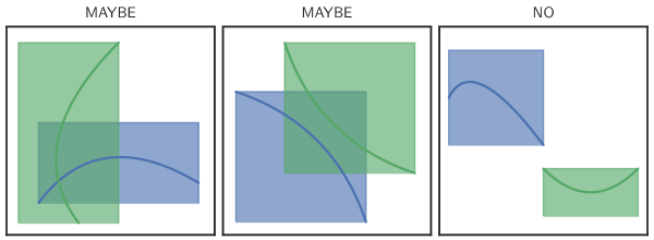
Figure A.1. Bounding box intersection predicate. This is a cheap way to conclude that two curves don’t intersect, though it inherently is susceptible to false positives.

In the Bézier subdivision algorithm, we first check if the bounding boxes for the curves are disjoint (Figure A.1). We use the bounding boxes rather than the convex hulls since they are easier to compute and the intersections of boxes are easier to check. If they are disjoint, the pair can be rejected. If not, each curve $\mathcal{C}=b\left(\left[0,1\right]\right)$ is split into two halves by splitting the unit interval: $b\left(\left[0,\frac{1}{2}\right]\right)$ and $b\left(\left[\frac{1}{2},1\right]\right)$ (Figure A.2).

Figure A.2. Bézier curve subdivision.

Figure A.3. Bézier subdivision algorithm.

As the subdivision continues, some pairs of curve segments may be kept around that won’t lead to an intersection (Figure A.3). Once the curve segments are close to linear within a given tolerance (Figure A.4), the process terminates.

Figure A.4. Subdividing until linear within tolerance.

Once both curve segments are linear (to tolerance), the intersection is approximated by intersecting the lines connecting the endpoints of each curve segment. This approximation is used as a starting point for Newton’s method, to find a root of $F(s,t)=b_{0}(s)-b_{1}(t)$. Since $b_{0}(s),b_{1}(t)\in\mathbf{R}^{2}$ we have Jacobian $J=\left[\begin{array}[]{c c}b_{0}^{\prime}(s)&-b_{1}^{\prime}(t)\end{array}\right]$. With these, Newton’s method is

$$\left[\begin{array}[]{c c}s_{n+1}&t_{n+1}\end{array}\right]^{T}=\left[\begin{array}[]{c c}s_{n}&t_{n}\end{array}\right]^{T}-J_{n}^{-1}F_{n}.$$ (A.1)

This also gives an indication why convergence issues occur at non-transveral intersections: they are exactly the intersections where the Jacobian is singular.

A.2. Intersecting Bézier Triangles

The chief difficulty in intersecting two surfaces is intersecting their edges, which are Bézier curves. Though this is just a part of the overall algorithm, it proved to be the most difficult to implement ([Her17]). So the first part of the algorithm is to find all points where the edges intersect (Figure A.5).

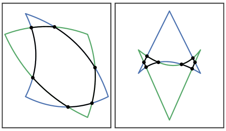
Figure A.5. Edge intersections during Bézier triangle intersection.

To determine the curve segments that bound the curved polygon region(s) (see Section 2.6 for more about curved polygons) of intersection, we not only need to keep track of the coordinates of intersection, we also need to keep note of which edges the intersection occurred on and the parameters along each curve. With this information, we can classify each point of intersection according to which of the two curves forms the boundary of the curved polygon (Figure A.6). Using the right-hand rule we can compare the tangent vectors on each curve to determine which one is on the interior.

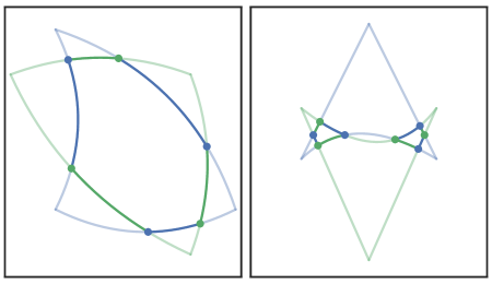
Figure A.6. Classified intersections during Bézier triangle intersection.

This classification becomes more difficult when the curves are tangent at an intersection, when the intersection occurs at a corner of one of the surfaces or when two intersecting edges are coincident on the same algebraic curve (Figure A.7).

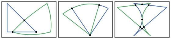
Figure A.7. Bézier triangle intersection difficulties.

In the case of tangency, the intersection is non-transversal, hence has infinite condition number. In the case of coincident curves, there are infinitely many intersections (along the segment when the curves coincide) so the subdivision process breaks down.

A.2.1. Example

Consider two Bézier surfaces (Figure A.8)

$$b_{0}(s,t)=\left[\begin{array}[]{c}8s\\ 8t\end{array}\right]\qquad b_{1}(s,t)=\left[\begin{array}[]{c}2(6s+t-1)\\ 2(8s^{2}+8st-8s+3t+2)\end{array}\right]$$ (A.2)

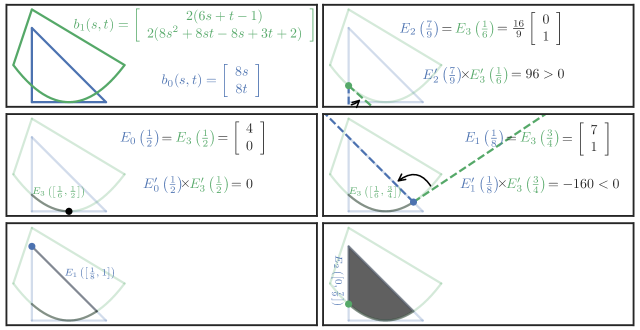
Figure A.8. Surface Intersection Example

In the first step we find all intersections of the edge curves

$$E_{0}(r)=\left[\begin{array}[]{c}8r\\ 0\end{array}\right],E_{1}(r)=\left[\begin{array}[]{c}8(1-r)\\ 8r\end{array}\right],E_{2}(r)=\left[\begin{array}[]{c}0\\ 8(1-r)\end{array}\right],\\ E_{3}(r)=\left[\begin{array}[]{c}2(6r-1)\\ 4(2r-1)^{2}\end{array}\right],E_{4}(r)=\left[\begin{array}[]{c}10(1-r)\\ 2(3r+2)\end{array}\right],E_{5}(r)=\left[\begin{array}[]{c}-2r\\ 2(5-3r)\end{array}\right].$$ (A.3)

We find three intersections and we classify each of them by comparing the tangent vectors

$$I_{1}:E_{2}\left(\frac{7}{9}\right)=E_{3}\left(\frac{1}{6}\right)=\frac{16}{9}\left[\begin{array}[]{c}0\\ 1\end{array}\right]\Longrightarrow E_{2}^{\prime}\left(\frac{7}{9}\right)\times E_{3}^{\prime}\left(\frac{1}{6}\right)=96$$ (A.6)

$$I_{2}:E_{0}\left(\frac{1}{2}\right)=E_{3}\left(\frac{1}{2}\right)=\left[\begin{array}[]{c}4\\ 0\end{array}\right]\Longrightarrow E_{0}^{\prime}\left(\frac{1}{2}\right)\times E_{3}^{\prime}\left(\frac{1}{2}\right)=0$$ (A.9)

$$I_{3}:E_{1}\left(\frac{1}{8}\right)=E_{3}\left(\frac{3}{4}\right)=\left[\begin{array}[]{c}7\\ 1\end{array}\right]\Longrightarrow E_{1}^{\prime}\left(\frac{1}{8}\right)\times E_{3}^{\prime}\left(\frac{3}{4}\right)=-160.$$ (A.12)

From here, we construct our curved polygon intersection by drawing from our list of intersections until none remain.

• First consider $I_{1}$. Since $E_{2}^{\prime}\times E_{3}^{\prime}>0$ at this point, then we consider the curve $E_{3}$ to be interior.

• After classification, we move along $E_{3}$ until we encounter another intersection: $I_{2}$

• $I_{2}$ is a point of tangency since $E_{0}^{\prime}\left(\frac{1}{2}\right)\times E_{3}^{\prime}\left(\frac{1}{2}\right)=0$. Since a tangency has no impact on the underlying intersection geometry, we ignore it and keep moving.

• Continuing to move along $E_{3}$, we encounter another intersection: $I_{3}$. Since $E_{1}^{\prime}\times E_{3}^{\prime}<0$ at this point, we consider the curve $E_{1}$ to be interior at the intersection. Thus we stop moving along $E_{3}$ and we have our first curved segment: $E_{3}\left(\left[\frac{1}{6},\frac{3}{4}\right]\right)$

• Finding no other intersections on $E_{1}$ we continue until the end of the edge. Now our (ordered) curved segments are:

  $$E_{3}\left(\left[\frac{1}{6},\frac{3}{4}\right]\right)\longrightarrow E_{1}\left(\left[\frac{1}{8},1\right]\right).$$ (A.13)

• Next we stay at the corner and switch to the next curve $E_{2}$, moving along that curve until we hit the next intersecton $I_{1}$. Now our (ordered) curved segments are:

  $$E_{3}\left(\left[\frac{1}{6},\frac{3}{4}\right]\right)\longrightarrow E_{1}\left(\left[\frac{1}{8},1\right]\right)\longrightarrow E_{2}\left(\left[0,\frac{7}{9}\right]\right).$$ (A.14)

  Since we are now back where we started (at $I_{1}$) the process stops

We represent the boundary of the curved polygon as Bézier curves, so to complete the process we reparameterize ([Far01, Ch. 5.4]) each curve onto the relevant interval. For example, $E_{3}$ has control points $p_{0}=\left[\begin{array}[]{c}-2\\ 4\end{array}\right]$, $p_{1}=\left[\begin{array}[]{c}4\\ -4\end{array}\right]$, $p_{2}=\left[\begin{array}[]{c}10\\ 4\end{array}\right]$ and we reparameterize on $\alpha=\frac{1}{6},\beta=\frac{3}{4}$ to control points

$$q_{0} =E_{3}\left(\frac{1}{6}\right)=\frac{16}{9}\left[\begin{array}[]{c}0\\ 1\end{array}\right]$$ (A.17)

$$q_{1} =(1-\alpha)\left[(1-\beta)p_{0}+\beta p_{1}\right]+\alpha\left[(1-\beta)p_{1}+\beta p_{2}\right]=\frac{1}{6}\left[\begin{array}[]{c}21\\ -8\end{array}\right]$$ (A.20)

$$q_{2} =E_{3}\left(\frac{3}{4}\right)=\left[\begin{array}[]{c}7\\ 1\end{array}\right].$$ (A.23)

A.3. Bézier Triangle Inverse

The problem of determining the parameters $(s,t)$ given a point $\bm{p}=\left[\begin{array}[]{c c}x&y\end{array}\right]^{T}$ in a Bézier triangle can also be solved by using subdivision with a bounding box predicate and then Newton’s method at the end.

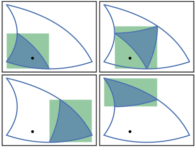
Figure A.9. Checking for a point $\bm{p}$ in each of four subregions when subdividing a Bézier triangle.

For example, Figure A.9 shows how regions of $\mathcal{U}$ can be discarded recursively until the suitable region for $(s,t)$ has a sufficiently small area. At this point, we can apply Newton’s method to the map $F(s,t)=b(s,t)-\bm{p}$. It’s very helpful (for Newton’s method) that $F:\mathbf{R}^{2}\longrightarrow\mathbf{R}^{2}$ since the Jacobian will always be invertible when the Bézier triangle is valid. If $\bm{p}\in\mathbf{R}^{3}$ then the system would be underdetermined. Similarly, if $\bm{p}\in\mathbf{R}^{2}$ but $b(s)$ is a Bézier curve then the system would be overdetermined.

Appendix B Allowing Tessellation with Inverted Triangles

Theorem B.1.

Consider three smooth curves $b_{0},b_{1},b_{2}$ that form a closed loop: $b_{0}(1)=b_{1}(0)$, $b_{1}(1)=b_{2}(0)$ and $b_{2}(1)=b_{0}(0)$. Take any smooth map $\varphi(s,t)$ on $\mathcal{U}$ that sends the edges to the three curves:

$$\varphi(r,0)=b_{0}(r),\quad\varphi(1-r,r)=b_{1}(r),\quad\varphi(0,1-r)=b_{2}(r)\quad\text{for }r\in\left[0,1\right].$$ (B.1)

Then we must have

$$2\int_{\mathcal{U}}\det(D\varphi)\left[F\circ\varphi\right]\,dt\,ds=\oint_{b_{0}\cup b_{1}\cup b_{2}}H\,dy-V\,dx$$ (B.2)

for antiderivatives that satisfy $H_{x}=V_{y}=F$.

When $\det(D\varphi)>0$, this is just the change of variables formula combined with Green’s theorem.

Proof.

Let $x(s,t)$ and $y(s,t)$ be the components of $\varphi$. Define

$$\Delta S=H(x,y)y_{s}-V(x,y)x_{s}\quad\text{and}\quad\Delta T=H(x,y)y_{t}-V(x,y)x_{t}.$$ (B.3)

On the unit triangle $\mathcal{U}$, Green’s theorem gives

$$\int_{\mathcal{U}}\left[\partial_{s}\Delta T-\partial_{t}\Delta S\right]\,dV=\oint_{\partial\mathcal{U}}\Delta S\,ds+\Delta T\,dt.$$ (B.4)

The boundary $\partial\mathcal{U}$ splits into the bottom edge $E_{0}$, hypotenuse $E_{1}$ and left edge $E_{2}$.

Since

$$E_{0}=\left\{\left[\begin{array}[]{c}r\\ 0\end{array}\right]\mid r\in\left[0,1\right]\right\}$$ (B.5)

we take $\varphi(r,0)=b_{0}(r)$ hence

$$dx=x_{s}\,dr,dy=y_{s}\,dr\Longrightarrow Hdx-Vdy=\Delta S\,dr.$$ (B.6)

We also have $ds=dr$ and $dt=0$ due to the parameterization, thus

$$\int_{E_{0}}\Delta S\,ds+\Delta T\,dt=\int_{r=0}^{r=1}\Delta S\,dr=\int_{b_{0}}H\,dx-V\,dy.$$ (B.7)

We can similarly verify that $\int_{E_{j}}\Delta S\,ds+\Delta T\,dt=\int_{b_{j}}H\,dx-V\,dy$ for the other two edges. Combining this with (B.4) we have

$$\int_{\mathcal{U}}\left[\partial_{s}\Delta T-\partial_{t}\Delta S\right]\,dV=\oint_{b_{0}\cup b_{1}\cup b_{2}}H\,dx-V\,dy.$$ (B.8)

To complete the proof, we need

$$\int_{\mathcal{U}}\left[\partial_{s}\Delta T-\partial_{t}\Delta S\right]\,dV=2\int_{\mathcal{U}}\det(D\varphi)\left[F\circ\varphi\right]\,dV$$ (B.9)

but one can show directly that

$$\partial_{s}\Delta T-\partial_{t}\Delta S=2\left(x_{s}y_{t}-x_{t}y_{s}\right)F(x,y)=2\det(D\varphi)\left[F\circ\varphi\right]. \blacksquare$$

References

- [Ber87] Marsha J. Berger. On conservation at grid interfaces. SIAM Journal on Numerical Analysis, 24(5):967–984, Oct 1987.
- [BR78] I. Babuška and W. C. Rheinboldt. Error estimates for adaptive finite element computations. SIAM Journal on Numerical Analysis, 15(4):736–754, 1978.
- [CDS99] Xiao-Chuan Cai, Maksymilian Dryja, and Marcus Sarkis. Overlapping nonmatching grid mortar element methods for elliptic problems. SIAM Journal on Numerical Analysis, 36(2):581–606, Jan 1999.
- [CGQ18] Xiaofeng Cai, Wei Guo, and Jingmei Qiu. A high order semi-Lagrangian discontinuous Galerkin method for the two-dimensional incompressible Euler equations and the guiding center Vlasov model without operator splitting. ArXiv e-prints, Apr 2018.
- [CH94] G. Chesshire and W. D. Henshaw. A scheme for conservative interpolation on overlapping grids. SIAM Journal on Scientific Computing, 15(4):819–845, Jul 1994.
- [Che74] Patrick Chenin. Quelques problèmes d’interpolation à plusieurs variables. Theses, Institut National Polytechnique de Grenoble - INPG ; Université Joseph-Fourier - Grenoble I, June 1974. Université : Université scientifique et médicale de Grenoble et Institut National Polytechnique.
- [CMOP04] David E. Cardoze, Gary L. Miller, Mark Olah, and Todd Phillips. A Bézier-based moving mesh framework for simulation with elastic membranes. In Proceedings of the 13th International Meshing Roundtable, IMR 2004, Williamsburg, Virginia, USA, September 19-22, 2004, pages 71–80, 2004.
- [DK87] John K. Dukowicz and John W. Kodis. Accurate conservative remapping (rezoning) for Arbitrary Lagrangian-Eulerian computations. SIAM Journal on Scientific and Statistical Computing, 8(3):305–321, May 1987.
- [DKR12] Veselin A. Dobrev, Tzanio V. Kolev, and Robert N. Rieben. High-order curvilinear finite element methods for Lagrangian hydrodynamics. SIAM J. Sci. Comput., 34(5):B606–B641, 2012.
- [Duk84] John K Dukowicz. Conservative rezoning (remapping) for general quadrilateral meshes. Journal of Computational Physics, 54(3):411–424, Jun 1984.
- [Dun85] D. A. Dunavant. High degree efficient symmetrical Gaussian quadrature rules for the triangle. International Journal for Numerical Methods in Engineering, 21(6):1129–1148, Jun 1985.
- [Far91] R.T. Farouki. On the stability of transformations between power and bernstein polynomial forms. Computer Aided Geometric Design, 8(1):29–36, Feb 1991.
- [Far01] Gerald Farin. Curves and Surfaces for CAGD, Fifth Edition: A Practical Guide (The Morgan Kaufmann Series in Computer Graphics). Morgan Kaufmann, 2001.
- [Flo03] Michael S. Floater. Mean value coordinates. Computer Aided Geometric Design, 20(1):19–27, Mar 2003.
- [FM11] P.E. Farrell and J.R. Maddison. Conservative interpolation between volume meshes by local Galerkin projection. Computer Methods in Applied Mechanics and Engineering, 200(1-4):89–100, Jan 2011.
- [FPP+09] P.E. Farrell, M.D. Piggott, C.C. Pain, G.J. Gorman, and C.R. Wilson. Conservative interpolation between unstructured meshes via supermesh construction. Computer Methods in Applied Mechanics and Engineering, 198(33-36):2632–2642, Jul 2009.
- [GKS07] Rao Garimella, Milan Kucharik, and Mikhail Shashkov. An efficient linearity and bound preserving conservative interpolation (remapping) on polyhedral meshes. Computers & Fluids, 36(2):224–237, Feb 2007.
- [GT82] William J. Gordon and Linda C. Thiel. Transfinite mappings and their application to grid generation. Applied Mathematics and Computation, 10-11:171–233, Jan 1982.
- [HAC74] C.W Hirt, A.A Amsden, and J.L Cook. An Arbitrary Lagrangian-Eulerian computing method for all flow speeds. Journal of Computational Physics, 14(3):227–253, Mar 1974.
- [Her17] Danny Hermes. Helper for Bézier curves, triangles, and higher order objects. The Journal of Open Source Software, 2(16):267, Aug 2017.
- [IK04] Armin Iske and Martin Käser. Conservative semi-Lagrangian advection on adaptive unstructured meshes. Numerical Methods for Partial Differential Equations, 20(3):388–411, Feb 2004.
- [JH04] Xiangmin Jiao and Michael T. Heath. Common-refinement-based data transfer between non-matching meshes in multiphysics simulations. International Journal for Numerical Methods in Engineering, 61(14):2402–2427, 2004.
- [JM09] Claes Johnson and Mathematics. Numerical Solution of Partial Differential Equations by the Finite Element Method (Dover Books on Mathematics). Dover Publications, 2009.
- [KLS98] Deok-Soo Kim, Soon-Woong Lee, and Hayong Shin. A cocktail algorithm for planar Bézier curve intersections. Computer-Aided Design, 30(13):1047–1051, Nov 1998.
- [KS08] M. Kucharik and M. Shashkov. Extension of efficient, swept-integration-based conservative remapping method for meshes with changing connectivity. International Journal for Numerical Methods in Fluids, 56(8):1359–1365, 2008.
- [MD92] Dinesh Manocha and James W. Demmel. Algorithms for intersecting parametric and algebraic curves. Technical Report UCB/CSD-92-698, EECS Department, University of California, Berkeley, Aug 1992.
- [MM72] R. McLeod and A. R. Mitchell. The construction of basis functions for curved elements in the finite element method. IMA Journal of Applied Mathematics, 10(3):382–393, 1972.
- [MS03] L.G. Margolin and Mikhail Shashkov. Second-order sign-preserving conservative interpolation (remapping) on general grids. Journal of Computational Physics, 184(1):266–298, Jan 2003.
- [MXS09] S. E. Mousavi, H. Xiao, and N. Sukumar. Generalized Gaussian quadrature rules on arbitrary polygons. International Journal for Numerical Methods in Engineering, 2009.
- [PBP09] P.-O. Persson, J. Bonet, and J. Peraire. Discontinuous Galerkin solution of the Navier–Stokes equations on deformable domains. Computer Methods in Applied Mechanics and Engineering, 198(17-20):1585–1595, Apr 2009.
- [Per98] Alain Perronnet. Triangle, tetrahedron, pentahedron transfinite interpolations. application to the generation of c0 or g1-continuous algebraic meshes. In Proc. Int. Conf. Numerical Grid Generation in Computational Field Simulations, Greenwich, England, pages 467–476, 1998.
- [PUdOG01] C.C. Pain, A.P. Umpleby, C.R.E. de Oliveira, and A.J.H. Goddard. Tetrahedral mesh optimisation and adaptivity for steady-state and transient finite element calculations. Computer Methods in Applied Mechanics and Engineering, 190(29-30):3771–3796, Apr 2001.
- [PVMZ87] J Peraire, M Vahdati, K Morgan, and O.C Zienkiewicz. Adaptive remeshing for compressible flow computations. Journal of Computational Physics, 72(2):449–466, Oct 1987.
- [SN90] T.W. Sederberg and T. Nishita. Curve intersection using Bézier clipping. Computer-Aided Design, 22(9):538–549, Nov 1990.
- [SP86] Thomas W Sederberg and Scott R Parry. Comparison of three curve intersection algorithms. Computer-Aided Design, 18(1):58–63, Jan 1986.
- [Wac75] Eugene Wachspress. A Rational Finite Element Basis. Academic Press, Amsterdam, Boston, 1975.
- [WFA+13] Z.J. Wang, Krzysztof Fidkowski, Rémi Abgrall, Francesco Bassi, Doru Caraeni, Andrew Cary, Herman Deconinck, Ralf Hartmann, Koen Hillewaert, H.T. Huynh, Norbert Kroll, Georg May, Per-Olof Persson, Bram van Leer, and Miguel Visbal. High-order CFD methods: current status and perspective. International Journal for Numerical Methods in Fluids, 72(8):811–845, Jan 2013.
- [Zlá73] Miloš Zlámal. Curved elements in the finite element method. I. SIAM Journal on Numerical Analysis, 10(1):229–240, Mar 1973.
- [Zlá74] Miloš Zlámal. Curved elements in the finite element method. II. SIAM Journal on Numerical Analysis, 11(2):347–362, Apr 1974.