Forward modelling of brightness variations in Sun-like stars

Abstract

Context. The latitudinal distribution of starspots deviates from the solar pattern with increasing rotation rate. Numerical simulations of magnetic flux emergence and transport can help model the observed stellar activity patterns and the associated brightness variations.

Aims. We set up a composite model for the processes of flux emergence and transport on Sun-like stars to simulate stellar brightness variations for various levels of magnetic activity and rotation rates.

Methods. Assuming that the distribution of magnetic flux at the base of the convection zone follows solar scaling relations, we calculate the emergence latitudes and tilt angles of bipolar regions at the surface for various rotation rates, using thin-flux-tube simulations. Taking these two quantities as input to a surface flux transport (SFT) model, we simulate the diffusive-advective evolution of the radial field at the stellar surface, including effects of active region nesting.

Results. As the rotation rate increases, (1) magnetic flux emerges at higher latitudes and an inactive gap opens around the equator, reaching a half-width of $20^{\circ}$ for $8\Omega_{\sun}$; and (2) the tilt angles of freshly emerged bipolar regions show stronger variations with latitude. Polar spots can form at $8\Omega_{\sun}$ by accumulation of follower-polarity flux from decaying bipolar regions. From $4\Omega_{\sun}$ to $8\Omega_{\sun}$, the maximum spot coverage changes from 3 to 20%, respectively, compared to 0.4% in the solar model. Nesting of activity can lead to strongly non-axisymmetric spot distributions.

Conclusions. On Sun-like stars rotating at $8\Omega_{\sun}$ ($P_{\rm rot}\simeq 3$ days), polar spots can form, owing to higher levels of flux emergence rate and tilt angles. Defining spots by a threshold field strength yields global spot coverages that are roughly consistent with stellar observations.

1 Introduction

The advent of space-borne photometry, which is designed primarily to detect extrasolar planets, has made short-term stellar activity signals measurable (Koch et al., 2010). Brightness variations in Sun-like stars on timescales ranging from hours to decades are driven by convective flows and magnetic fields at the surface, while the observed patterns of variability also depend on the stellar rotation and related quantities (Aigrain et al., 2004; Shapiro et al., 2014, 2017).

Dark spots and bright faculae observed on the Sun are formed by relatively strong magnetic flux concentrations threading the photosphere. To investigate radiative variations driven by magnetic activity and rotation on Sun-like stars, it is important to numerically simulate the distribution and the evolution of surface magnetic fields at large scales.

The latitudinal distribution of starspots is one of the extensively studied features of magnetic activity on rapidly rotating cool stars, via Doppler and Zeeman-Doppler imaging (Strassmeier, 2009; Donati & Landstreet, 2009). For Sun-like stars in particular, the mean latitude of cool spots and magnetic fields has been observed to increase with the rotation rate. Spots near or at the rotational poles are observed on rapidly rotating Sun-like stars with rotation periods below about 3 days (Jeffers et al., 2002; Marsden et al., 2006; Järvinen et al., 2007; Waite et al., 2015).

As a possible explanation for polar spots, Schüssler & Solanki (1992) suggested a mechanism in which the action of the axially directed Coriolis force in the rotating frame of a rising flux tube becomes comparable to or even dominates the outward buoyancy force for sufficiently fast rotation. Schüssler et al. (1996) demonstrated how faster rotation deflects rising tubes towards high latitudes on Sun-like stars, and Granzer et al. (2000) obtained latitudinal distributions for a range of stellar masses.

A surface mechanism which can also contribute to the formation of polar spots was suggested by Schrijver & Title (2001) using a random-walk model of flux dispersal and transport. In this model, a strong high-latitude concentration of magnetic fields of a single polarity was formed by the trailing polarities of bipolar regions when the flux emergence rate was 30 times the solar value. A ring-like structure was formed around a polar spot of opposite polarity, which had a much longer decay time than what a diffusion model would infer.

Another attempt was made by Işık et al. (2007b), who used a diffusive surface flux transport (SFT) model subject to observed stellar surface differential rotation estimates and stellar radii. They suggested that the long lifetimes of polar spots can be explained by the mid-latitude emergence of a large bipolar region with a large tilt angle, presumably owing to strong action of the Coriolis effect. In both Schrijver & Title (2001) and Işık et al. (2007b), a largely unipolar polar spot was produced by the diffusion of flux from the follower-polarities of bipolar magnetic regions (BMRs) at low or medium latitudes.

Holzwarth et al. (2006) also used an SFT model to show that a sufficiently fast poleward meridional flow at the surface can also lead to polar spots, but with intermingled polarities. In an attempt to reproduce the flip-flop activity variations that have been reported for some active stars (Berdyugina, 2005), Elstner & Korhonen (2005) applied a non-axisymmetric mean-field dynamo model, which produced an asymmetric distribution of magnetic field concentrations near the rotational poles.

Schüssler et al. (1996) modelled the latitudinal distribution of emerging flux on solar-mass stars, and Işık et al. (2007a, 2011) studied the combined effects of the dynamo, emergence, and SFT processes on stellar cycles. It is known that the average inclination of bipolar magnetic regions with respect to the east-west direction (the tilt angle) is crucial in maintaining the solar activity cycle (Baumann et al., 2004; Jiang et al., 2010). However, a systematic modelling of Sun-like stars with physically consistent computation of tilt angles and the subsequent surface flux transport has not yet been undertaken.

To better understand the implications of the rotation-activity relation not too far from the solar regime and to provide a testing platform of forward modelling for photometric reconstructions, here we construct a modelling framework. It incorporates the observed properties of the solar cycle, the effects of rotation on rising flux tubes in the convection zone, and surface flux transport. In this paper, we present the method and discuss the impact of increasing rotation rate and activity on the surface patterns of magnetic flux. A following paper will be devoted to syntheses of light curves based on the magnetic flux emergence (Sect. 2.2) and transport models (Sect. 2.3) presented here. The purpose of the model presented here is restricted to reproducing brightness variations of Sun-like stars in high-precision data such as from Kepler (Koch et al., 2010) and TESS (Ricker et al., 2015), particularly from very short timescales up to several stellar rotations. We do not, however, rule out a later extension to also model spectroscopic (e.g. radial velocity) and spectropolarimetric changes by including horizontal fields. In Sect. 3 we present results from our scaled stellar models, namely temporal and latitudinal patterns of activity. The limitations of the model and the relevance of our results with respect to the observations of active Sun-like stars is discussed in Sect. 4.

2 Model setup

To model the emergence and the evolution of the surface magnetic field, we first generated an 11-year semi-synthetic sunspot group record based on the statistics of solar cycle 22 (Sect. 2.1.1). With increasing stellar rotation rate, we linearly scaled the flux emergence rate, in agreement with the observed rotation-activity relation. Stronger solar cycles are known to show a tendency for higher mean emergence latitudes (Solanki et al., 2008; Jiang et al., 2011). We therefore used an empirical relation to extrapolate the mean latitude of emergence to higher activity levels (Sect. 2.1.2). We assumed that the resulting distribution represents the butterfly diagram of flux-tube eruptions at the base of the convection zone of a G2V-type star with a given activity level. Using flux-tube simulations, we then computed the emergence latitudes and tilt angles of rising loops for a given stellar rotation rate (Sect. 2.2). A schematic presentation of the algorithm is given in detail in Appendix B.

The latitudinal distribution of emerging flux is therefore determined by two independent effects in our approach: $(i)$ The base latitudinal distribution changes with the flux emergence rate (extrapolation of the empirical solar relation between the activity level and the mean latitude); and $(ii)$ the rotation rate affects the action of the Coriolis force, which tends to deflect rising flux tubes poleward.

The resulting starspot emergence records are then used as input to the SFT model to obtain the evolution of surface magnetic flux (Sect. 2.3). In the following sub-sections we describe the various steps in this chain in greater detail.

2.1 Synthetic starspot group records

2.1.1 The input solar cycle

Using the RGO/SOON records between 1700 and 2010, Jiang et al. (2011, hereafter JCSS11) found statistical relationships between various characteristics of sunspot groups. They generated a semi-synthetic Spot Group Record (SGR) based on these relationships. We adopted the solar SGR generation procedures described in JCSS11 and Cameron et al. (2016, hereafter CJS16; see their Sect. 2.2) to simulate a relatively strong, artificial cycle lasting about 11 years. We describe the details of this procedure in Appendix A.

In summary, the synthetic cycle module provides the following quantities related to sunspot group emergence as a function of time (cycle phase): the total number of sunspot groups (Eq. 3); the emergence times and latitudes, which are determined by the mean latitude of sunspot groups (Eqs. 4-5); the width of the latitudinal spread (Eq. 6); random longitudes (nesting is introduced in Sect. 2.1.3); sunspot group areas drawn from a composite empirical distribution (Eq. 7).

Instead of using the tilt angles synthesised within the JCSS11 model from empirical relationships, we use the results of the flux-tube simulations to be described in Sect. 2.2. For the solar case, the results are similar to the tilt angle relationship assumed by JCSS11, while for more rapidly rotating stars very different tilt angle distributions are obtained.

Having defined the base model of the solar cycle, we now describe how we determine the flux emergence rate and the mean latitude of flux eruption, for more active Sun-like stars.

2.1.2 Scaling the cycle on more active stars

To scale the stellar cycle amplitude, $S_{\star}$, we define $\tilde{s}\equiv S_{\star}/S_{\sun}$, where $S$ is in units of the maximum of the annual running mean of the sunspot group number, $S_{\sun}$ is set to 156, which is the observed value for Cycle 22 (see Appendix A.1), and $\tilde{s}$ is then a relative measure of the emergence frequency (or rate) of BMRs; for simplicity, this quantity will be called the emergence frequency or flux emergence rate (in solar units) throughout the rest of the paper, as they are proportional quantities. To evaluate $\tilde{s}$, we focused on two extreme cases: $(i)$ a constant $\tilde{s}=1$, to isolate the rotational effects on the (otherwise solar) emergence pattern; and $(ii)$ a linear scaling $\tilde{s}=\tilde{\omega}:=\Omega_{\star}/\Omega_{\sun}$, following the observed proportionality $Bf=50v_{\rm eq}$ between the field strength ($Bf$, where $f$ is the filling factor) and the equatorial rotational velocity $v_{\rm eq}$ of Sun-like stars, estimated by Reiners (2012). To first order, $Bf$ is proportional to the total magnetic flux on the stellar disc. The scaling therefore provides a rough representation of the rotation-activity relationship of G dwarfs.

The effect that stronger solar cycles start at higher latitudes has already been considered by JCSS11. We extrapolated this effect to higher activity levels ($\tilde{s}>1$) and expressed the mean latitude of flux eruptions from the base of the stellar convection zone, $\langle\lambda\rangle_{\star}$, by modifying Eq. (5), as

$$\langle\lambda\rangle_{\star}=12.2+k\tilde{s}S_{\sun},$$ (1)

where we assumed $k=0.022$ for $\tilde{s}<8$, as in Eq. (5). We chose $k=0.014$ for $\tilde{s}=8$ to limit the maximum latitude of the input cycle to $73^{\circ}$. This roughly corresponds to the high-latitude edge of the main region of instability of flux tubes (see Sect. 2.2.1).

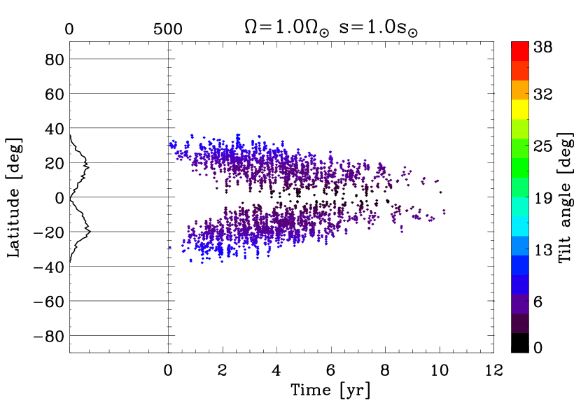
Figure 1: Semi-synthetic emergence record (SGR) for solar cycle 22, using emergence latitudes and tilt angles resulting from the remapping procedure for the solar rotation and flux emergence rate $(\tilde{\omega},\tilde{s})=(1.0,1.0)$. The colour bar shows the tilt angles with a rather high saturation level, so that the tilt angles can be compared with faster-rotating cases. The plot on the left shows the histogram of emergence latitudes.

(a)

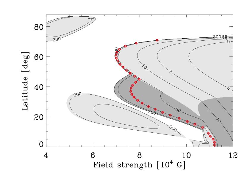
(b)

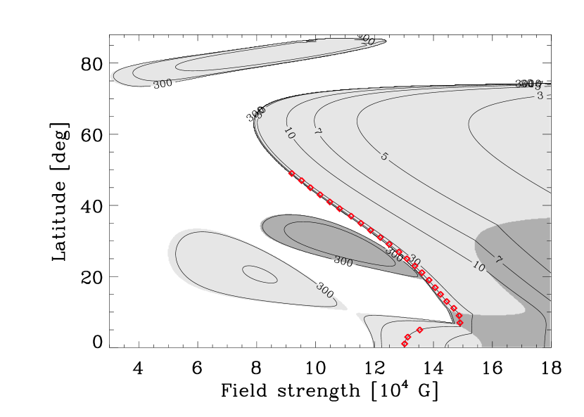
(c)

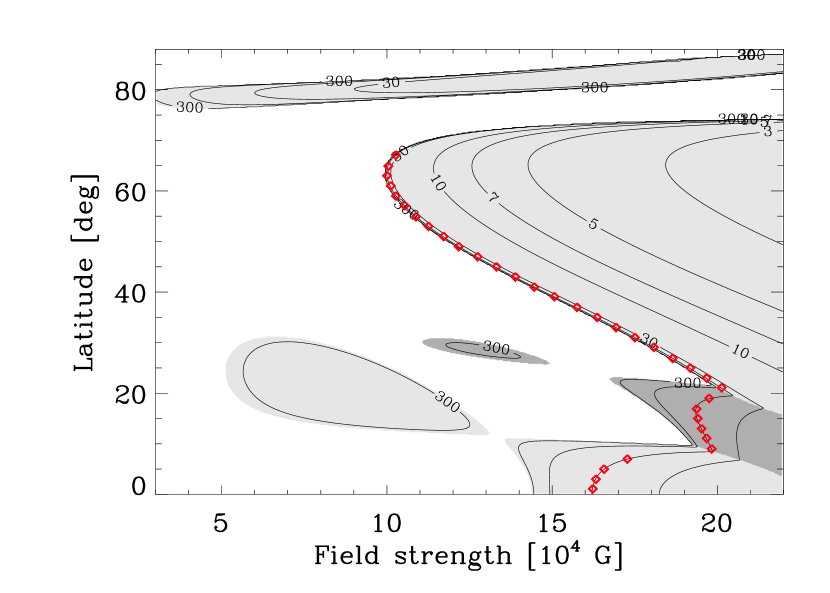
(d)

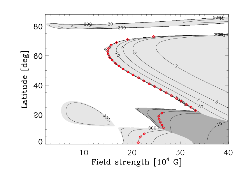
Figure 2: The initial latitudes and field strengths of flux tubes (red diamonds) chosen for flux-tube rise computations, plotted over linear stability diagrams for flux tubes at the middle of the overshoot region, for (a) $\tilde{\omega}=1$, (b) $\tilde{\omega}=2$, (c) $\tilde{\omega}=4$, and (d) $\tilde{\omega}=8$, with differential rotation $\Delta\Omega_{\star}=\Delta\Omega_{\sun}$. The contour lines denote the growth time in days. The linearly stable regime is shown in white, and the unstable regime is shaded with light grey where the fastest-growing mode is $m=1$, and with dark-grey for $m=2$. The red diamonds show the initial tube parameters chosen for the numerical simulations, at a growth time of 50 days.

Rather than assuming the surface emergence record described above to represent the distribution at the base of the convection zone, we corrected the eruption latitudes at the base of the convection zone for the weak poleward deflection of rising flux tubes at the solar rotation rate (see Appendix B).

2.1.3 Nesting of active regions

It is known that sunspot groups tend to emerge within ‘nests’ of activity (e.g. Castenmiller et al., 1986). To simulate the observed clumping of active-region emergence, we modified the longitudes and latitudes obtained in the previous steps by setting a probability that a given BMR would be part of a nest, which we call nesting probability (Appendix C). When this effect is included, the resulting cycle variation of low-order multipoles such as the equatorial dipole as well as the open flux better represent the observed variations.

Figure 1 shows the resulting solar reference butterfly diagram with $(\tilde{\omega},\tilde{s})=(1.0,1.0)$, with a nesting probability of 70%. The only significant difference from the synthetic cycle-22 butterfly diagram of the JCSS11 model is the clustered emergence pattern.

2.2 The rise of flux tubes in the convection zone

We model the latitudinal distribution of emerging magnetic flux on Sun-like stars using numerical simulations of buoyantly rising magnetic flux tubes. We adopt the thin flux tube approximation (Spruit, 1981) and model flux tubes leading to sunspot groups as initially toroidal flux rings in mechanical equilibrium (Caligari et al., 1998) in the form given by Ferriz-Mas & Schüssler (1995) and Caligari et al. (1995). At the equilibrium state, the flux tube is assumed to lie in the stably stratified overshoot region at the base of a solar-like, non-local-mixing-length convection zone model, which is adopted from Skaley & Stix (1991).

We take the angular rotation rate $\Omega$ as a function of radius $r$ and latitude $\lambda$,

$$\Omega(r,\lambda)/\Omega_{\star} = 1+2\frac{c_{3}}{\tilde{\omega}}-\left[1+{\rm erf}\left(\frac{r-r_{0}}{d}\right)\right]$$ (2)

$$\cdot\frac{1}{\tilde{\omega}}\left(c_{1}\sin^{4}\lambda+c_{2}\sin^{2}\lambda+c_{3}\right),$$

where $\Omega_{\star}$ is the equatorial rotation rate at the stellar surface, $c_{1}=0.0876$, $c_{2}=0.0535$, and $c_{3}=-0.0182$. The base of the convective overshoot region in the stratification model is at $r_{0}=0.724R_{\sun}$; it is taken as the centre of the tachocline here. Furthermore, $d=0.075R_{\sun}$ is the width of the error function defining the thickness of the tachocline and the constants $(c_{1},c_{2},c_{3},d)$ are chosen such that Eq. (2) closely mimics helioseismic inversions of solar internal rotation (Schou et al., 1998). Observational studies indicate that surface differential rotation increases rather weakly with the rotation rate as $\Delta\Omega_{\star}\propto\Omega^{n}_{\star}$, where $n$ was estimated to be 0.15 by Barnes et al. (2005), and 0.2 for G stars by Balona & Abedigamba (2016). For simplicity, we set $\Delta\Omega_{\star}=\Delta\Omega_{\sun}$ in both the radial and latitudinal directions. The factor $\tilde{\omega}^{-1}$ and the term $2c_{3}\tilde{\omega}^{-1}$ in Eq. (2) account for keeping the same (solar) differential rotation rate in both the radius and latitude, as $\Omega_{\star}$ increases.

2.2.1 Initial properties of flux tubes

Following Ferriz-Mas & Schüssler (1995), we solve the sixth-order dispersion relation for linear perturbations of a toroidal flux ring in mechanical equilibrium, taking the thermodynamical quantities from the stratification model and the rotation profile from Eq. (2).

Figure 2 shows the linear stability diagrams for toroidal flux tubes in the middle of the overshoot region ($r_{\rm mid}=0.728R_{\sun}$) as a function of the initial latitude $\lambda_{0}$ and the field strength $B_{0}$, for different rotation rates and the same Sun-like stratification. In light- and dark-shaded regions, the fastest-growing wave mode has an azimuthal wavenumber of $m=1$ and $m=2$, respectively. The radial location is about 5000 km beneath the base of the convection zone (the term ‘base’ signifies the depth at which the convective heat flux changes its sign). The red dots in Fig. 2 show $\lambda_{0}$ and $B_{0}$ of flux tubes chosen for the non-linear simulations (Sect. 2.2.2) with $2^{\circ}$ latitudinal steps, all corresponding to a characteristic linear growth time of 50 days. This growth time ensures that the tubes are sufficiently close to the onset of instability and that the Joy’s law resulting from the simulations for $\tilde{\omega}=1$ matches well with the solar observations. We did not consider the islands of instability because (1) the corresponding growth time is not reached in the lower-latitude island; and (2) the high-latitude island is not reached by the input butterfly diagram in any case, except for $\tilde{s}=8$. To be conservative, we preferred to limit the simulations to the main region of instability by decreasing the factor $k$ in Eq. (1) for $\tilde{s}=8$.

The maximum latitude at step I is $73^{\circ}$ for $\tilde{s}=8$ (Sect. 2.1.2). To cover the entire latitude range in the input solar cycle for all flux emergence rates, we set up flux-tube simulations with initial latitudes at the base of the convection zone up to $\lambda_{0}=73^{\circ}$ for $\tilde{\omega}=1$, to move from step I to II. This is the same maximum latitude as for the input model at the surface because the flux tubes rise almost radially for $\tilde{\omega}=1$, especially at high latitudes (Fig. 3).

The stability diagrams in Fig. 2 show that the onset of instability is shifted towards higher field strengths for higher rotation rates, by a factor of about 3 for $\tilde{\omega}=8$, compared to the solar value, owing to the enhanced Coriolis force component directed towards the rotation axis, which has a stabilising effect. The dynamics of the tube is governed predominantly by the buoyancy, curvature, and Coriolis forces in the rotating frame. The tube radius is relevant only for the drag force, which only weakly affects the resulting emergence properties. For all the simulations, we set the initial cross-sectional radius to 2000 km, about 3.6 % of the local pressure scale height. With this radius and the initial field strengths corresponding to a growth time of 50 days (Fig. 2), the magnetic flux within a tube is typically about $10^{22}$ Mx for $\tilde{\omega}=1$ and $3\times 10^{22}$ Mx for $\tilde{\omega}=8$. The flux-tube rise simulations serve only to obtain emergence latitudes and tilt angles, which are only slightly affected by the initial tube radius via the drag force.

2.2.2 Simulations of flux tube emergence

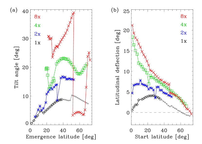
Figure 3: (a) The tilt angle of emerging flux loops vs. their emergence latitude for $\tilde{\omega}=1$ (black diamonds), $\tilde{\omega}=2$ (blue asterisks), $\tilde{\omega}=4$ (green squares), and $\tilde{\omega}=8$ (red crosses). (b) Latitudinal deflections (poleward is positive) as a function of the initial latitude at the base of the convection zone. The initial $\lambda_{0}$ and $B_{0}$ are as in Fig. 2. Emergence latitudes for which no active-region-sized BMR emerges for $(\tilde{\omega},\tilde{s})=(1,1)$ are shown by small grey diamonds (see text).

To model the rise of flux tubes through the convection zone, we carried out simulations starting from the initial parameters mentioned above (Sect. 2.2.1, see Fig. 2). We used the code developed by Moreno-Insertis (1986) and extended to three-dimensional (3D) geometry by Caligari et al. (1995). It solves the dynamical evolution of a one-dimensional (1D), initially toroidal ring of mass elements embedded in a 1D background stratification (Skaley & Stix, 1991) in the 3D Lagrangian frame. The mass elements are subject to body forces including the drag force, Lorentz force, and buoyancy, as well as the pseudo-forces induced by the Coriolis and centrifugal effects. The evolution of the tube is considered as an isentropic process. The magnetic flux and the integrity of the tube with its closed structure are also conserved. We chose $10^{3}$ mass elements for the flux tube, which is initially in mechanical equilibrium and subject to a linear combination of azimuthally periodic spatial perturbations with wave numbers in the range $1\leqslant m\leqslant 5$. Their magnitudes are $10^{-4}$ in units of the local pressure scale height, in each of the three dimensions. Unstable tubes experience magnetic buoyancy instability and develop loops that rise up to a heliocentric radial distance of about $0.98R_{\sun}$. At this point, the simulation halts owing to the ambient pressure scale height becoming comparable with the tube diameter, violating the thin-tube criterion. We roughly define this stage as the ‘emergence’ of the loop, though the loop is still under the surface. In general, the fastest-growing azimuthal wave mode in the non-linear simulations is consistent with the prediction of linear stability analysis (Fig. 2). When $m=2$, two buoyant loops form with a 180-degree phase difference, and one of them emerges before the other. The simulations are stopped at this point due to the thin-flux-tube criterion, so it is not possible to track the other emergence at the opposite longitudinal hemisphere. Therefore, our simulations may be somewhat underestimating the amount of magnetic flux that emerges at the stellar surface when $m=2$ is the dominant mode of instability.

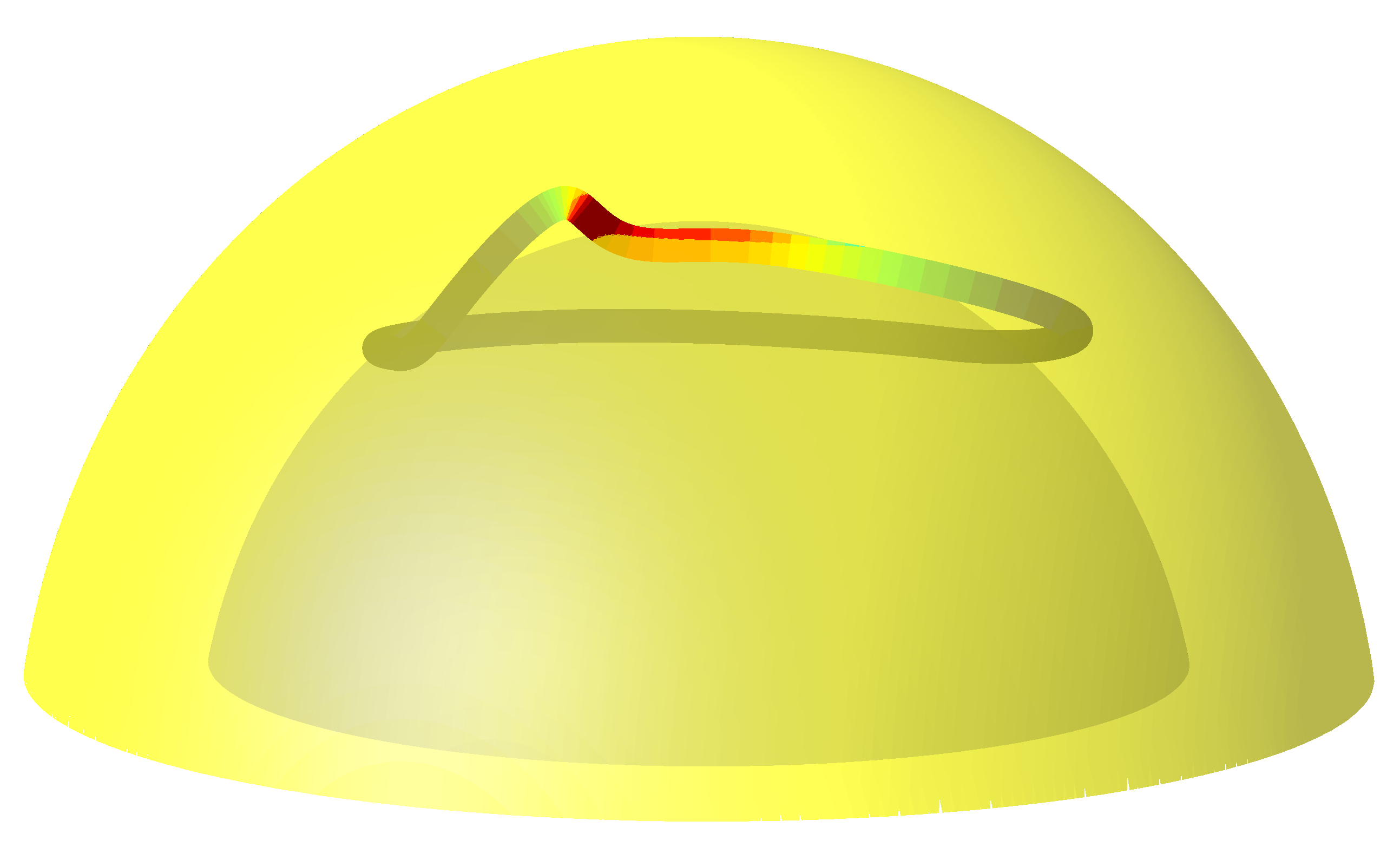
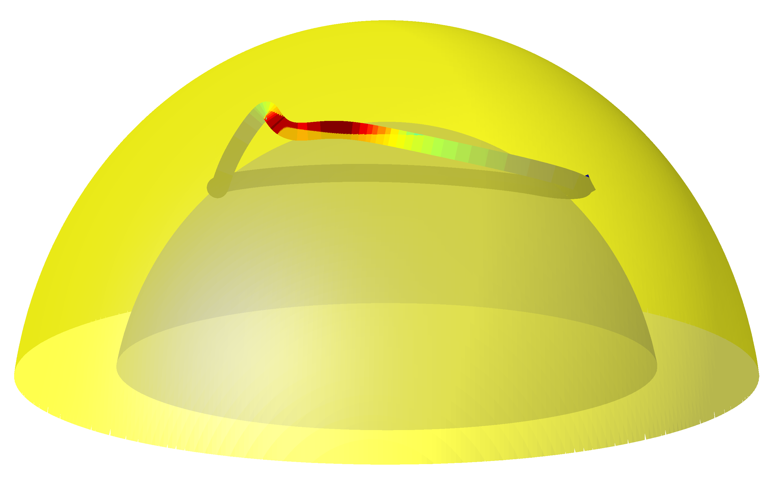
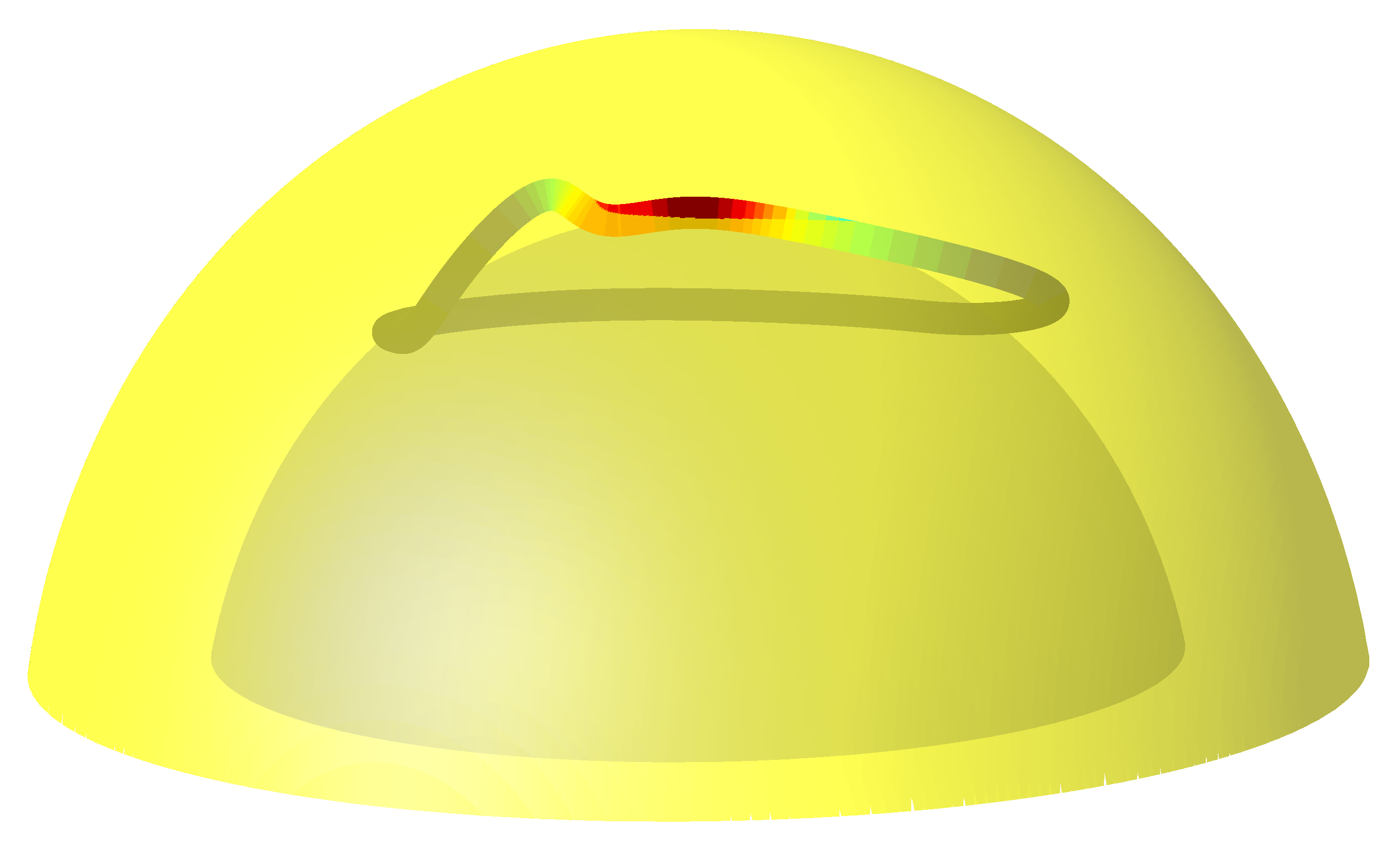
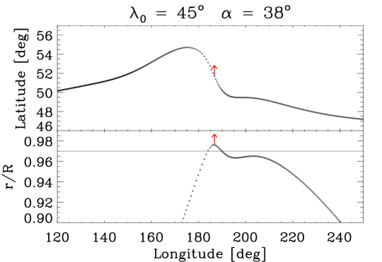
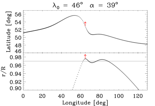
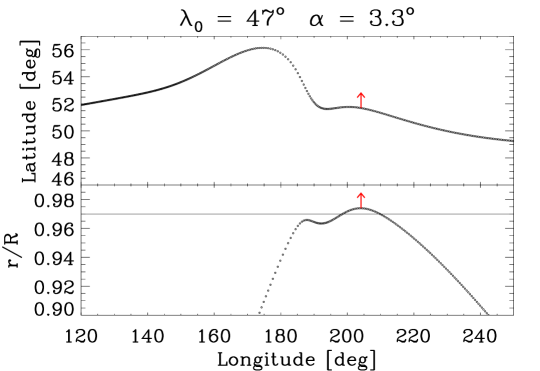
Figure 4: Geometry of three emerging flux loops with initial latitudes $45^{\circ}$ (left), $46^{\circ}$ (middle), and $47^{\circ}$ (right) at the base of the convection zone. In the upper panels, the inner sphere is drawn at $0.72R_{\sun}$, and the outer sphere at $0.97R_{\sun}$. The parts of the tube that are beneath the outer layer are shaded in grey, whereas the emerged parts are brighter. For each mass element of the tube, the colours denote the cross-sectional tube diameter (the redder the larger). Lower panels show the latitudinal and radial projections of the tubes, where each mass element is represented by a dot. The horizontal line on the radial profile corresponds to the location of the outer sphere ($0.97R_{\sun}$), where the tilt angle ($\alpha$) is measured from the footpoint locations. The red arrows denote the apex of each tube.

The initial $(\lambda_{0},B_{0})$ determined by the growth time of 50 days and the initial radial location are set such that the loops yield a realistic set of emergence latitudes and tilt angles for the Sun. The time between the initial state to the emergence, that is, including the development of the instability, ranges from a few hundred to a thousand days and increases with $\Omega_{\star}$. We measure the emergence latitude from the apex of the tube at the end of the simulation. We determine the tilt angle by using the longitudes and latitudes of the preceding and follower legs of the flux loop at $0.97R_{\sun}$. The results are roughly consistent with the tilt angles obtained from the slope of the tangent vector at the apex.

Figure 3 shows, as a function of the emergence latitude $\lambda_{e}$, the tilt angles $\alpha$ (this dependence is called Joy’s law in solar physics) and the latitudinal deflection $\lambda_{e}-\lambda_{0}$ as a function of the initial latitude, for different rotation rates. Simulations were made for the full range of latitudes in the case $\tilde{\omega}=1$, including latitudes where no emergence occurs in $(\tilde{\omega},\tilde{s})=(1,1)$ (smaller diamonds in Fig. 3). This additional latitude range was needed because we scaled the mean latitude of activity with $\tilde{s}$ in step I (Eq. 1), in accordance with the empirical solar model extrapolated to higher flux emergence rates. In general, both $\lambda_{e}$ and $\alpha$ increase with the rotation rate, owing to enhanced Coriolis force components in the rotating frame.

There are a few abrupt changes in $\alpha(\lambda_{e})$, which are also visible in $\lambda_{e}-\lambda_{0}$. To understand the origin of such features, we first eliminated the possibility of a numerical resolution issue. For this, we set up tubes with higher numbers of mass elements (up to 4000), but these runs converged to very similar values of emergence latitudes and tilt angles. Following additional simulations with slightly different initial field strengths, we found that these jumps were robust features. They are shaped by physical effects, that is, they represent regimes where different forces and/or different wave modes become dominant. For instance, the local peak in the tilt angle for $\tilde{\omega}=1$ at $\lambda_{e}\simeq 15^{\circ}$ occurs at the transition of the fastest-growing mode from $m=1$ to $m=2$ (see Fig. 2a).

To investigate the nature of the largest jump for $\tilde{\omega}=8$, we show in Fig. 4 the emergence phases of flux tubes starting at $\lambda_{0}=45^{\circ}$, $46^{\circ}$, and $47^{\circ}$, that is, roughly where the jump in the tilt angle at about $\lambda_{\rm e}=50^{\circ}$ occurs (see Fig. 3). The plots clearly depict the transition from the case when a highly tilted part of the tube emerges earlier (Fig. 4a), to the case when a much less tilted part emerges earlier (Fig. 4c). The radial and azimuthal projections of the tubes mark this transition clearly. The relative phase speeds of the two competing loops vary with $\lambda_{0}$, such that the low-tilt loop intrudes the high-tilt loop above a certain initial latitude of about $46^{\circ}$. The transition from partial to full intrusion is responsible for the low-tilt plateau in Fig. 3a, for $\lambda_{\rm e}$ between about $50^{\circ}$ and $65^{\circ}$. The two loops fully merge beyond $\lambda_{\rm e}=70^{\circ}$, where moderate tilts of about $22^{\circ}$ are reached (see Fig. 3a).

As an independent test, thin flux tube simulations for $\tilde{\omega}=8$ have been kindly made by M. Weber (priv. comm.) using the code developed by Fan et al. (1993). The only two differences with our setup were that she assumed rigid rotation for the stellar interior and started the tubes in the lower convection zone, where the superadiabaticity was positive. Nevertheless, the resulting latitude dependence of the tilt angle and the latitudinal deflection turned out to be qualitatively similar to our case for $\tilde{\omega}=8$. The distribution and amplitude of the abrupt variations in the tilt angle roughly agreed with each other in these two sets of independent simulations.

It is quite possible that both loops forming out of a single flux tube eventually emerge, producing active regions with quite different tilts. Hence, regions with systematically different tilts can coexist at nearly the same latitude on rapidly rotating stars. However, since the thin tube approximation does not allow us to continue the computations further, we have simply used the tilts of the region emerging first.

2.3 Surface flux transport

We used the solar and stellar SGRs described in Sect. 2.1 as input to the SFT model (see Jiang et al., 2014, for a review), for which we employed the code developed by Baumann et al. (2004). The code solves, with one-day steps, the magnetic induction equation at the solar/stellar surface, where the field is assumed to be purely radial. This allows us to consider the field as scalar, with a sign representing the magnetic polarity. This is a reasonable assumption for the kilo-Gauss fields on the Sun found in active region plage, solar network, and sunspot umbrae, though the geometry of the highly inclined fields in penumbrae is not taken into account. Because the purpose of this series of studies is to simulate brightness variations, we did not attempt to model the horizontal components of the magnetic field, for which the relationship with brightness variations in Sun-like stars is unclear. Exceptions are spot penumbrae, which can be treated as having a homogeneous brightness at the effective spatial resolution that can be reached in stellar observations. In the current endeavour to model brightness variations, we implicitly assume that larger-scale horizontal fields are transients that occur only during flux emergence, and neglect their signature in the brightness distribution on a stellar disc.

2.3.1 Properties of bipolar magnetic regions

In our SFT model, the distribution of the field on the solar surface is represented in terms of spherical harmonic functions, with a maximum degree of $l=64$, corresponding to a resolution at the level of supergranular cells on the Sun. The freshly emerged BMRs are defined as two circular regions of opposite polarity, with a fixed upper limit of the field strength, $B_{\rm max}$. The interpolarity distance (ranging between 3 and 10^∘) controls the size of each BMR, as the characteristic radius of each polarity is fixed at $4^{\circ}$. We adopt $B_{\rm max}=374$ G, which was determined by Cameron et al. (2010), who matched the variation of the total unsigned magnetic flux from an SFT simulation to magnetographic observations of the Sun from Mount Wilson and Wilcox Solar Observatories.

(a)

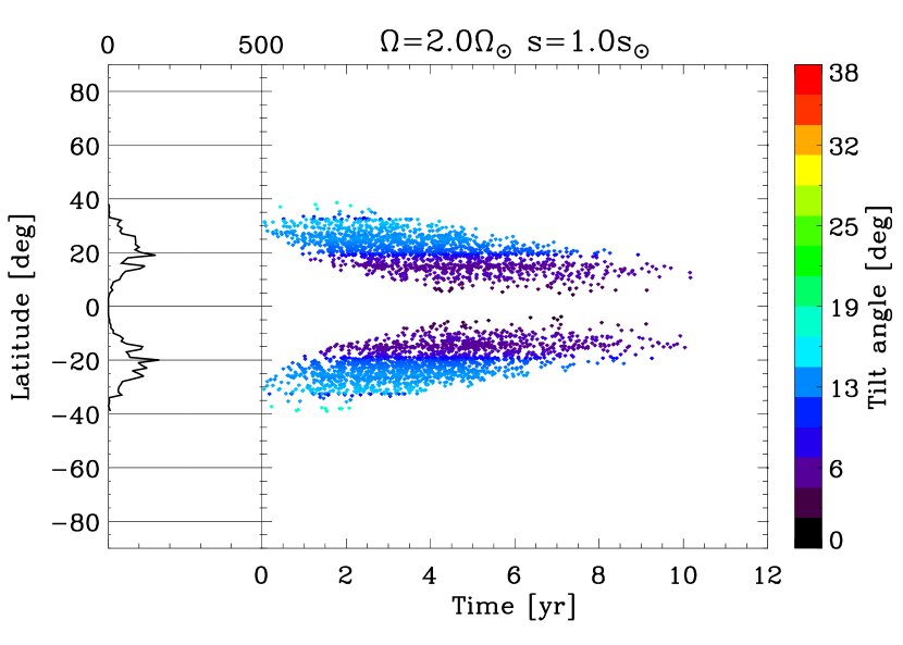
(b)

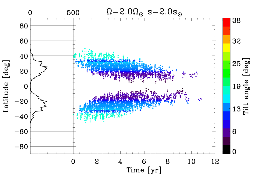
(c)

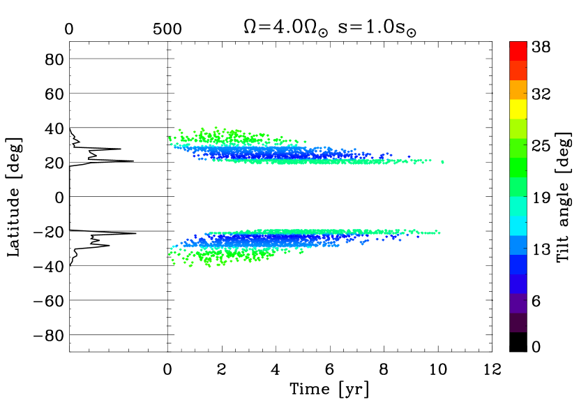
(d)

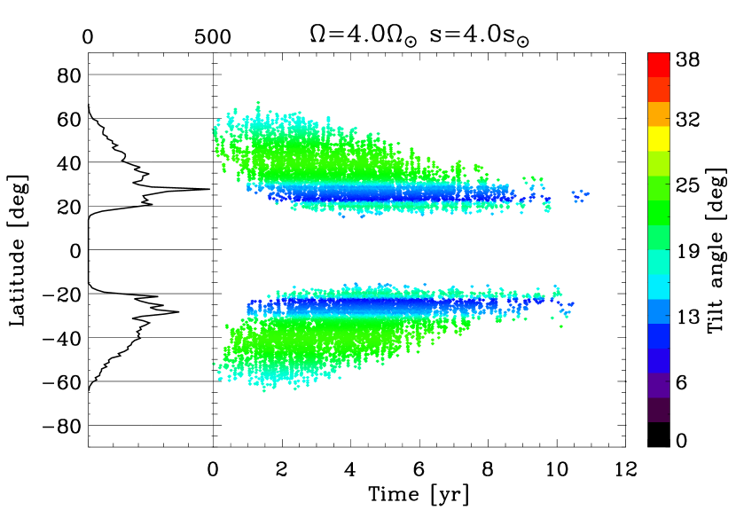
(e)

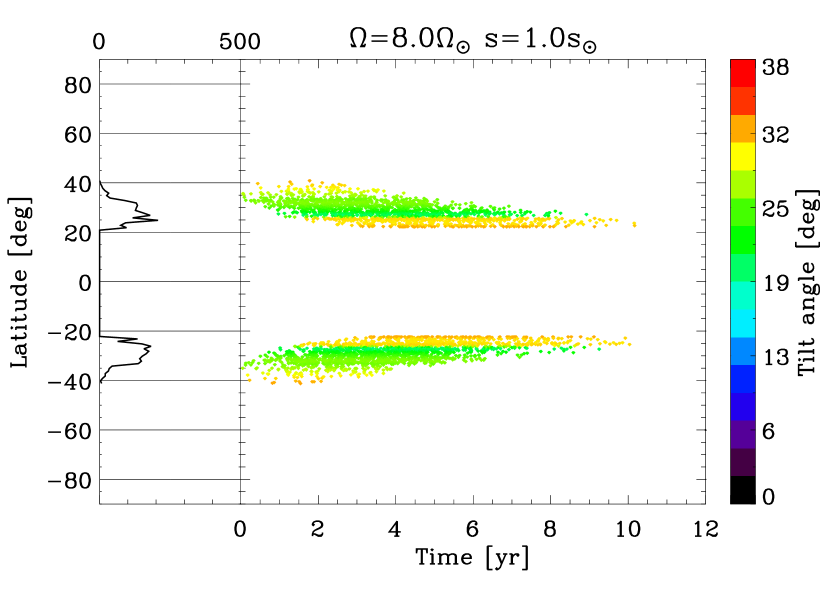
(f)

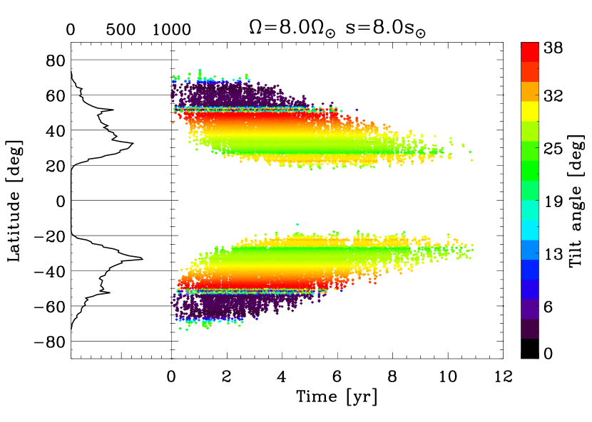
Figure 5: As in Fig. 1, but now for various sets of $(\tilde{\omega},\tilde{s})$ as indicated at the top of each panel. The left panels are for $\tilde{s}=1$ (solar emergence rate), and the right panels are for $\tilde{s}=\tilde{\omega}$.

(a)

(b)

(c)

(d)

2.3.2 Surface flows

The surface fields are subject to differential rotation and poleward meridional flow, which are assumed stationary, and follow the same profiles as in Baumann et al. (2004). The latitudinal shear considered in the SFT model is very similar to Eq. (2) at $r=R_{\sun}$. The difference does not affect the resulting surface flux distributions. The meridional flow reaches a poleward speed of 11 m s^-1 at mid-latitudes and ceases at $\lambda=\pm 75^{\circ}$. For the effects of smaller-scale flows (supergranulation), the SFT model considers the diffusion term in the induction equation, with a horizontal turbulent diffusivity of 250 km² s^-1 (Cameron et al., 2010) and a radial diffusivity of 25 km² s^-1 (Baumann et al., 2006).

2.3.3 Initial magnetic field

As the initial condition, we assume a dipolar field reaching $B_{\rm max}(t=0)=\pm 10\tilde{s}$ G at the poles, which takes into account the possibility of stronger initial axial dipole moments for higher levels of flux emergence rate, $\tilde{s}$.

The resulting time series of surface maps of the radial magnetic field are represented in the so-called Carrington frame, where the latitudes of about $\pm 5^{\circ}$ are at rest. We assumed that the SFT parameters were invariant for all sets of $(\tilde{\omega},\tilde{s})$, except for the initial field condition.

2.4 Summary of assumptions

Here we summarise our assumptions when modelling faster-rotating, more active suns.

1. The time-latitude distribution of flux tube eruptions at the base of the convection zone follows the statistical properties of the solar butterfly diagram (Sect. 2.1.1), with the cycle duration set to 11 years.

   1. The mean latitude of eruptions at the base follows the same linear scaling with the cycle strength, as observed on the solar surface (Sect. 2.1.2).

   2. The initial field strengths of erupting flux tubes correspond to a constant linear growth time (50 days) of the magnetic buoyancy instability (Fig. 2) at the middle of the convective overshoot layer near the base (Sect. 2.2.1).

2. The number of eruptions throughout the 11-year cycle scales linearly with the rotation rate, $\tilde{s}=\tilde{\omega}$, except for the comparison case $\tilde{s}=1$ (Sect. 2.1.2).

3. The stratification and the differential rotation ($\Delta\Omega$) in the convection zone are kept the same as in the solar model (Sect. 2.2).

4. The surface flux transport coefficients and the large-scale flows are the same as in the solar model (Sects. 2.3.1-2.3.2).

5. The initial surface field is dipolar with a peak unsigned strength (at the rotational poles) equal to $10\tilde{s}$ G (Sect. 2.3.3).

3 Results

3.1 Butterfly diagrams

Figure 5 shows the butterfly diagrams for six sets of $(\tilde{\omega},\tilde{s})$. For $\tilde{\omega}=$2, 4, and 8, we consider either a solar ($\tilde{s}=1$, left panels) or a scaled stellar ($\tilde{s}=\tilde{\omega}$, right panels) flux emergence rate (Sect. 2.1.2).

For $\tilde{s}=1$ (panels a, c, and e), the systematic increase of both the mean emergence latitude and the tilt angle with $\tilde{\omega}$ is evident, owing to stronger Coriolis acceleration of rising tubes. For $\tilde{s}=\tilde{\omega}$ (panels b, d, and f), the imposed increase in $\tilde{s}$ leads to a further increase in the mean latitude of activity, owing not only to the Coriolis effect, but also to the solar-like scaling of the mean latitude (Eq. 1), as can be seen in the associated latitude histograms. In addition, the gap of inactivity around the equator with $\tilde{\omega}$ widens. However, the gaps are not very different from each other in cases $\tilde{\omega}=4$ and 8 (see also Fig. 3b for comparison). The colours represent the tilt angles, as in Fig. 1. The abrupt changes in the tilt angle are visible at some latitudes (cf. Fig. 3a), especially for $(\tilde{\omega},\tilde{s})=(8,8)$.

3.2 Variation of surface magnetic activity

The synthetic emergence records presented in Sect. 3.1 are now provided as input to the SFT model. In the first set of simulations, we keep the solar flux emergence rate ($\tilde{s}=1$) and increase the rotation rate (Sect. 3.2.1). In the second set, we increase both quantities with $\tilde{s}=\tilde{\omega}$ (Sect. 3.2.2).

3.2.1 Solar flux emergence rate ($\tilde{s}=1$)

Figure LABEL:fig:fluxvar shows the 27-day averages of the unsigned flux over the stellar surface and the unsigned mean polar field strength (averaged over both polar caps, which are defined for $|\lambda|>75^{\circ}$) using the same colours as in Fig. 3. Taking $\lambda_{e}$ and $\alpha$ for $\tilde{\omega}>1$ with the solar flux emergence rate ($\tilde{s}=1$, Fig. LABEL:fig:fluxvara) leads to a total flux variation which increases only weakly with $\tilde{\omega}$. This enhancement of the flux is due to the systematic increase in the average tilt angles of emerging BMRs, which weakens flux cancellation over the polarity inversion line of each BMR. While the mean tilt angle $\langle\alpha\rangle$ increases from about $5^{\circ}$ to $30^{\circ}$, the latitudinal separation between the polarities increases with $\sin\langle\alpha\rangle$. The poleward deflection of rising loops indirectly contributes to the increase (with $\tilde{\omega}$) of flux for $\tilde{s}=1$: the emergence latitudes become more confined to a range where the latitudinal shear is stronger than at the solar activity belts. The strong differential rotation at the activity belt tends to disperse the opposite polarities at an even higher rate, immediately following any BMR emergence. This decreases the cancellation between the opposite polarities within the same BMR. Such self-cancellation accounts for a significant fraction of the initial flux decrease of a BMR.

The isolated effect of faster rotation for $\tilde{s}=1$ (Fig. 5 a, c, and e) is more conspicuous for the polar field amplitudes (Fig. LABEL:fig:fluxvarc), for which the increasing tilt angle is the major contributor. This leads to a larger latitudinal separation between the polarities of a BMR, allowing the meridional flow to transport a larger amount of the following polarity to the pole, while the leading polarity has more time to cancel with the field from other BMRs. The increasing latitudinal deflection produces the opposite effect for the polar field than for the total magnetic flux: by shifting both polarities of each BMR towards higher latitudes, it decreases the efficiency of cross-equatorial flux cancellation. However, the effect remains sufficiently weak for up to $\tilde{\omega}=8$, for which most BMRs still emerge well below the latitude of the fastest meridional flow ($\sim 37^{\circ}$). Another consequence of the increase in $\langle\alpha\rangle$ is that the polar field reverses its polarity and reaches its peak value earlier for increasing $\tilde{\omega}$.

3.2.2 Flux emergence rate scaled with rotation ($\tilde{s}=\tilde{\omega}$)

For the set $\tilde{s}=\tilde{\omega}$ (Fig. 5b, d, and f), the amplitudes of both the total flux and the polar field increase more strongly with $\tilde{\omega}$ than in the case of $\tilde{s}=1$ (Fig. LABEL:fig:fluxvarb,d). Still, the total flux and the polar field increase at a rate lower than the scaling $\tilde{s}=\tilde{\omega}$ itself. The polar field reversals occur earlier owing to increasing average tilt angles, but there is no difference in the reversal time from $(\tilde{\omega},\tilde{s})=(4,4)$ to (8,8). The reason is that a significant amount of BMRs in the case (8,8) emerge within the low-tilt plateau above $\lambda\sim 50^{\circ}$ (see Figs. 3a and 5f). In this case, $\tilde{s}=8$ does not provide sufficient contribution to the global (axial) dipole moment to reverse it earlier than in the case (4,4). We note that in (8,8) the initial polar field that has to be reversed is stronger by a factor of two, relative to (4,4), owing to our assumption $B_{\rm max}(t=0)=\pm 10\tilde{s}$ G.

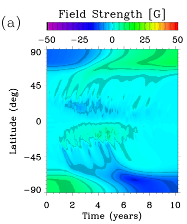
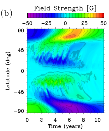
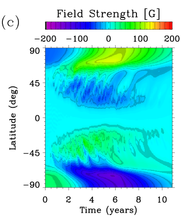
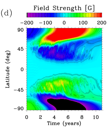
Figure 7: Time-latitude diagrams of azimuthally averaged surface magnetic field for (a) $\tilde{\omega}=1$, (b) $\tilde{\omega}=2$, (c) $\tilde{\omega}=4$, and (d) $\tilde{\omega}=8$. For all cases, $\tilde{s}=\tilde{\omega}$. We note the different saturation levels of the colour scale.

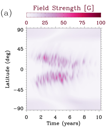
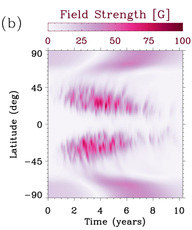
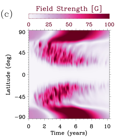
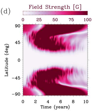
Figure 8: Time-latitude diagrams of azimuthally averaged $|B_{r}|$ for (a) $\tilde{\omega}=1$, (b) $\tilde{\omega}=2$, (c) $\tilde{\omega}=4$, and (d) $\tilde{\omega}=8$. $\tilde{s}=\tilde{\omega}$ for all cases. Here, the saturation levels are all 100 G.

The rotational dependencies of the total surface flux and the polar flux are shown in Fig. LABEL:fig:fluxvare in terms of the time integral of both quantities. The dependence is almost linear for both $\tilde{s}=1$ and $\tilde{s}=\tilde{\omega}$, with similar slopes. In the latter case the time-integrated total flux scales as $c\tilde{\omega}$, with $c\approx 0.9$. This is expected from the linearity of the SFT process (Schrijver, 2001). The non-linear dependence of the BMR dipole moments on $\tilde{\omega}$ does not lead to a significant deviation here. Eight-times-faster rotation leads to a change in the cumulative polar flux of about $2\times 10^{24}$ Mx, which is about 8 % of the corresponding change in the cumulative surface flux. It should be noted, however, that the cumulative polar flux scales non-linearly with $\tilde{\omega}$, at a gradually increasing rate, owing to rotationally induced effects. The contributors to the positive correlation between the two quantities are now both the increased latitudinal separation between polarities (increasing mean tilt angle) and the imposed dependence $\tilde{s}=\tilde{\omega}$.

3.2.3 Magnetic butterfly diagrams for $\tilde{s}=\tilde{\omega}$

Figure 7 shows the longitudinal averages of the surface magnetic field for $\tilde{s}=\tilde{\omega}$ models, as a function of time. One can directly see the effect of increased tilt angles (i.e. latitudinal separation of the preceding and the follower polarities) on the quicker formation of a stronger polar field. For the more rapidly rotating stars, the increase in both the flux emergence rate and the tilt angles cause the time at which the polar field reaches its maximum value to converge towards the time of the maximum total surface flux.

Figure 8 shows the unsigned radial field at the surface, averaged over longitude, for the cases shown in Fig. 7. In this way, it is easier to compare the distribution of the activity belts with that of polar fields, because the arithmetic cancellation of opposite-polarity fields is avoided during longitudinal averaging. It is evident that mid-latitude activity strengthens considerably for $\tilde{\omega}=4$ and 8. Above $(\tilde{\omega},\tilde{s})=(4,4)$, the polar fields start to become comparable with the mid-latitude activity, and they also become dominant for an increasingly larger fraction of the cycle.

3.3 The distribution and coverage of starspots ($\tilde{s}=\tilde{\omega}$)

To define spot areas from surface magnetic maps, we followed the simplest approach of setting a threshold to the magnetic field strength. All pixels with a field strength above the threshold are considered to belong to spots. We determine the threshold value from the condition that the time average of the spot coverage through the cycle, $\langle a_{s}\rangle_{\rm cyc}$, roughly corresponds to the cycle-averaged umbral spot coverage observed on the Sun, which is about 0.002. Using this criterion, we have found a threshold of 187 G, corresponding to about 50 % of $B_{\rm max}$ defined in Sect. 2.3. We have then used this threshold to determine the latitudinal distribution of the spot coverage for all four rotation rates with $\tilde{s}=\tilde{\omega}$.

(a)

(b)

(c)

(d)

Figure LABEL:fig:spotlatsa-d shows time-averaged latitudinal profiles of spot occupancy as a fraction of the stellar surface area. The area fractions were calculated by counting the pixels above the threshold, taking into account their areas on a spherical grid. In most observational studies, a factor of $\cos\lambda$ is used when estimating the fractional spot area per latitude bin. This means that our profiles are comparable with such latitudinal profiles presented in the literature (e.g. Järvinen et al., 2007; Waite et al., 2017). When the spot occupancy would be given as a fraction of the latitudinal band area, however, the polar spot of the case $(\tilde{\omega},\tilde{s})=(8,8)$ would lead to a much larger coverage near the pole than at mid-latitudes. The spot coverage over the whole stellar surface, averaged over the whole activity cycle (darker curves), $\langle a_{s}\rangle_{\rm cyc}$, increases from the solar value of 0.2% to 0.4% for $\tilde{\omega}=2$, 1.2% for $\tilde{\omega}=4$, and 10% for $\tilde{\omega}=8$. For comparison, one-year averages centred at the activity maximum are also given (lighter colours). There is a marked tendency for the mean latitude and the latitudinal spread of starspots to increase with $\tilde{\omega}$ and $\tilde{s}$. The mean latitude at each hemisphere increases, owing to the Coriolis deflection of rising flux and the enhanced poleward transport of highly tilted source regions. The increase in the latitudinal spread is led by ($i$) higher flux emergence rate, ($ii$) the scaling of mean latitude with $\tilde{s}$ (Eq. 5), and ($iii$) weaker flux cancellation between opposite polarities of BMRs, owing to a higher average tilt angle. It is evident from Fig. LABEL:fig:spotlatsd ($\tilde{\omega}=8$) that, through the flux transport at sufficiently high $\tilde{\omega}$ and $\tilde{s}$, spotted regions are formed at even higher latitudes than their emergence latitudes. Such starspots are formed by signed magnetic flux being transported towards higher latitudes and concentrated there. Figure LABEL:fig:spotlatse shows the variation of the surface coverage of starspots for all the four cases above. The cycle means are about one-third of the annual means around maxima, except for the the case (1,1), for which the ratio is about 0.5.

Figure 10 shows snapshot surface distributions of signed field from the maximum phases of activity, corresponding to each of the considered rotation rates, for the case $\tilde{s}=\tilde{\omega}$. The polar fields become stronger for higher $(\tilde{\omega},\tilde{s})$, while the activity belts move towards higher latitudes. A strong unipolar polar cap forms for $\tilde{\omega}=8$, but it is surrounded by patches of opposite-polarity field, owing to the leading polarities of freshly emerged, tilted BMRs. A conspicuous feature is visible for $\tilde{\omega}=8$: $dB/d\lambda$ changes its sign at $\lambda\simeq 75^{\circ}$, where the poleward meridional flow piles up the field diffusing from lower latitudes. In the later stages of the cycle, this ring-like structure diffuses to form a circular region peaking at the rotational pole.

a

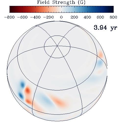
b

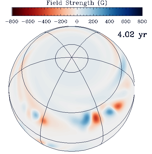
c

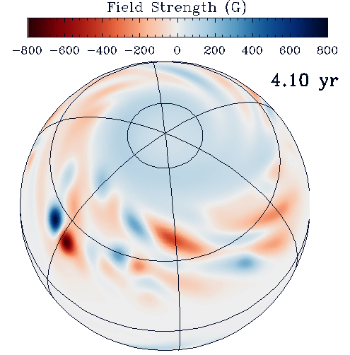
d

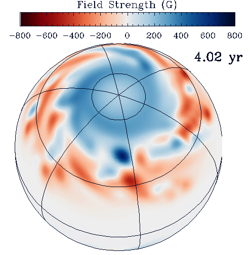
Figure 10: Snapshots of magnetic field strength from the runs for $\tilde{\omega}=1,2,4,8$ (panels a to d), corresponding to the cycle maximum in each case. The inclination angle of the rotation axis with respect to the line of sight is $30^{\circ}$. The latitudinal circles are drawn at $\lambda=37.5^{\circ}$, where the poleward flow speed has a maximum, and at $\lambda=75^{\circ}$, above which it is assumed to be zero.

In Fig. 11 we show the unsigned magnetic field strength, filtered with the threshold of 187 G. These snapshots can be seen as approximations of intensity images by omitting the limb-darkening and facular brightening effects. The strengthening of the polar field and of mid-latitude activity with increasing $\tilde{\omega}$ is visible. Based on the spot threshold field strength, the polar spot forms only for $\tilde{\omega}=8$, and it shows the same ring-shaped pattern as in Fig. 10 with occasional plumes in the direction of the equator. Here, the solar case exhibits too large ‘sunspots’, though the total area fraction is solar-like. This is because the resolution of the SFT model is not high enough to resolve typical sunspots. In addition, the saturation level for the unsigned field is only 400 G, about an order of magnitude below the average field strength of sunspot umbrae. Consequently, the simulated stellar images presented here are meant to represent a medium-resolution picture of spots on Sun-like stars. The resolution is therefore between those of solar full-disc white-light images and those produced by Doppler imaging (e.g. Solanki & Unruh, 2004). A more rigourous treatment of spot areas is beyond the scope of this study, and will be employed in the next paper for proper modelling of brightness variations.

a

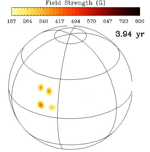
b

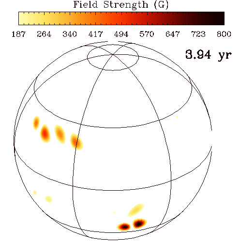
c

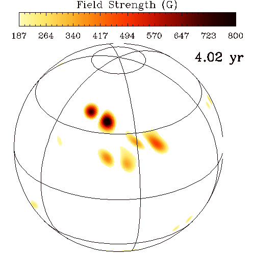
d

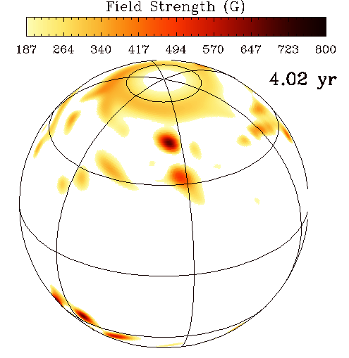
Figure 11: As in Fig. 10, but for the unsigned magnetic field strength with an inclination of $60^{\circ}$. The maps show the distribution of starspots, which are defined as all pixels above the threshold of 187 G.

It is known that faster-rotating G stars generally show stronger brightness variability (McQuillan et al., 2014). In this context, nesting of active regions can have an influence on the variability amplitudes on timescales comparable with the rotation period. This is because the surface distribution of spots would become less homogeneous in longitude (rotational phase), when spots tend to emerge within nests. As a visual demonstration of the effect of nesting, we show in Fig. 12 pole-on views ($i=0$) of our case $(\tilde{\omega},\tilde{s})=(8,8)$ at three different phases of the activity cycle, for random (unnested) and strongly nested cases, where the nesting probability was chosen to be $p=0.7$ (same as in all the previous figures). We also display the signed field distributions corresponding to the nested case, for the overall field geometry and strength to be evaluated. Without forced nesting, the spot distribution appears more axisymmetric. With nesting, the highly non-axisymmetric spot distribution is likely to induce larger-amplitude brightness variations on rotational timescales.

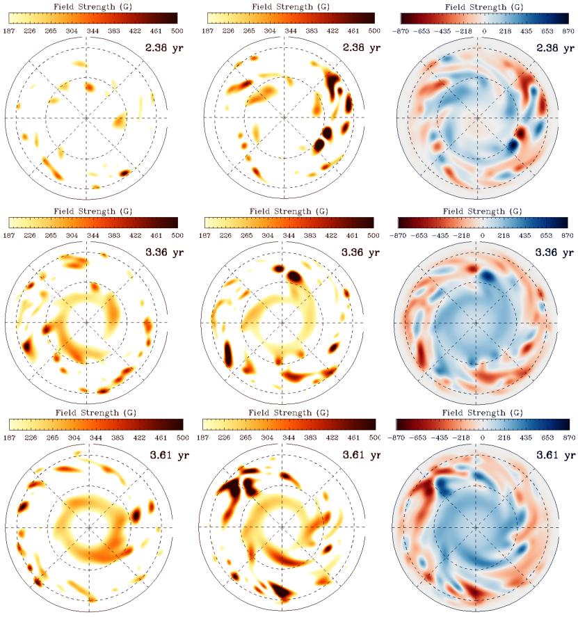
Figure 12: Pole-on views of the radial field, representing spot distributions for unnested (left column) and nested (middle column) cases for $(\tilde{\omega},\tilde{s})=(8,8)$. The right column shows the corresponding signed magnetic field strength for the nested case, with a colour saturation at $\pm 870\leavevmode\nobreak\ G.$ Dotted circles represent the latitudes at $30^{\circ}$ and $60^{\circ}$. We note that the spots are defined above 187 G.

4 Discussion

We have developed a two-part model, to provide time-resolved maps of the radial magnetic field on Sun-like stars with rotation rates in the range $\Omega_{\sun}\leqslant\Omega\leqslant 8\Omega_{\sun}$, which corresponds to a (sidereal) equatorial rotation period range of 25 to 3 days. The platform developed here will be used in the forward modelling of brightness variations on timescales covering active region evolution, stellar rotation, and the activity cycle (the second paper in this series). It also has the potential to be used in synthesising spectra covering photospheric lines used in Doppler imaging.

The thin flux-tube simulations successfully model the basic dynamical aspects of the emergence of large-scale flux loops in the case of the Sun, despite several idealisations involved (Caligari et al., 1995). Distributions of tilt angles in faster-rotating suns have not been well investigated so far, despite their potential effects on the distribution and evolution of surface magnetic flux. We have demonstrated in this study that these effects can be significant. Though we focused on the photospheric distribution of large-scale radial fields, the dynamical effects of increasing rotation rate on the emerging flux would certainly have implications for coronal magnetic structure (Gibb et al., 2016).

The model provides clues about how patterns of stellar activity are likely to change with increasing rotation and flux-emergence rates. We assumed that the time-latitude pattern of flux eruptions at the base follows the solar butterfly-diagram trends. Because currently there is no empirical evidence favouring any specific pattern for the internal toroidal field for $\tilde{\omega}>1$, we preferred this simple and conservative approach to also test the applicability of the solar paradigm. Therefore, the only change in the dynamo with increasing rotation rate is that it produces more toroidal flux, which reaches higher latitudes at the base of the convection zone.

We extrapolated the empirical relation for the mean latitude of the solar butterfly pattern to higher levels of activity, as if a solar cycle had an amplitude $\tilde{s}$ times its Cycle-22 level. This was done to obtain the base distributions of such very strong cycles before they rise to the surface, for $1\Omega_{\sun}$ (step II in Appendix B). This step is necessary because observations show that sunspots appear at higher average latitudes during stronger cycles (Solanki et al., 2008; Jiang et al., 2011). However, it is also possible that in real stars the deviation from a solar-like butterfly diagram at the base of the convection zone can be significant, especially for more rapid rotators. In future work, extrapolation of composite or Babcock-Leighton type dynamo models to faster rotating Sun-like stars can be employed (Işık et al., 2011; Karak et al., 2014) to obtain an estimate of the butterfly diagram of the internal toroidal field more consistently (see also Warnecke, 2018).

Our simulations show that the polar field exhibits the following trends with increasing $\tilde{\omega}$: $(i)$ it strengthens relative to lower-latitude activity, and $(ii)$ it reverses its polarity increasingly earlier with respect to the activity maximum (Fig. LABEL:fig:fluxvard), in spite of the fact that the initial polar field was scaled with the rotation rate. The first trend results from two effects, namely higher tilt angles and stronger activity. The second tendency can lead to an earlier amplification of the toroidal field by the action of differential rotation on the poloidal field. In addition to meridional circulation and dynamo effects (Jouve et al., 2010; Işık et al., 2011), it can thus contribute to shortening the cycle period for more active stars.

There are two competing effects in our models which determine the polar field amplitude: the increasing tilt angles (with rotation rate) tend to amplify the developing polar fields, whereas the gap of inactivity opening around the equator (with faster rotation) leads to weaker cross-equatorial preceding-polarity flux cancellation, which limits the growth of a strong polar cap. We speculate that there is a critical rotation rate at which the two following timescales become comparable: the timescale for the magnetic flux of each polarity within a BMR to diffuse and cancel each other, and the timescale for the preceding-polarity flux from a typical BMR to diffuse and cancel with the preceding-polarity flux from a corresponding BMR from the opposite hemisphere. Beyond such a critical rotation rate, polar fluxes would be saturated, provided that we are using the same solar transport parameters. Such high rotation rates and activity levels are beyond the scope of this paper.

Another effect that can hinder the formation of circumpolar spots is related to the dynamo process. If the cycle period decreases and cycle overlap increases significantly with the rotation rate, then the polar fields resulting from surface flux transport may not reach sufficient strengths to form spots before the subsequent cycle peaks (see the Sun-like model with $P_{\rm rot}=2$ days in Işık et al., 2011). However, circumpolar spots are indeed observed on some Doppler images of rapidly rotating Sun-like stars. Future observations and modelling of cycles on Sun-like stars should address this issue.

Our $(\tilde{\omega},\tilde{s})=(8,8)$ case can be compared to the Sun-like (G1.5V) star EK~Draconis, which has $\tilde{\omega}\simeq 8.8$. This star also exhibits a polar spot and mid-latitude activity in several Doppler and Zeeman-Doppler images (Järvinen et al., 2007; Waite et al., 2017). This qualitative agreement is gratifying. Furthermore, its mean umbral spot coverage is estimated to be in the range 0.25-0.40 based on TiO-band observations by O’Neal et al. (2004), whereas our model for (8,8) gives a cycle mean of 0.07 and a maximum of 0.20. We consider these values to be in reasonable agreement given the rather simple thresholding used to determine spot areas, and also that we scale the amount of magnetic flux linearly with the rotation rate.

We applied nesting of BMR emergence as observed on the Sun to more active stars. The resulting SFT simulations led to substantial rotational asymmetry in the starspot distributions on active stars. If the observed starspots are in fact low-resolution manifestations of such active nests (Özavcı et al., 2018) then the observed sizes and lifetimes of these structures may not be indicative of the intrinsic sizes and lifetimes of their constituent spots (see Işık et al., 2007b, for solutions of monolithic vs. clustered unipolar spot diffusion).

Zeeman-Doppler imaging studies show that the azimuthal component of the magnetic field strengthens and becomes comparable to or even exceeds the radial field for very active Sun-like stars. Our SFT model considers only the radial component of the field. Inclusion of the horizontal components (e.g. Gibb et al., 2016; Lehmann et al., 2017) represents a considerable extension of our current understanding, and they are beyond the present scope of modelling brightness variations of moderately active Sun-like stars. These components will therefore be introduced in a future study.

Our assumption that the meridional flow and differential rotation profiles are identical to those on the Sun has an effect on the resulting latitudinal distribution of the magnetic field. For instance, we expect that a meridional flow reaching up to latitudes higher than our assumed $75^{\circ}$ would lead to a field peaking at the poles earlier in a given cycle. However, such details should not dramatically change the production of a polar spot. Deviations of these profiles from the solar patterns would affect the evolution of flux in various latitudinal zones. Alternative profiles from theoretical models of flow fields as a function of the rotation rate can be used in our model (Küker et al., 2011; Kitchatinov & Olemskoy, 2012).

Finally, we note that it might be possible to reproduce the observed surface patterns of activity starting from different combinations of dynamo-generated toroidal field patterns, initial flux-tube conditions, and large-scale flows in the convective envelope. However, our aim has not been to seek the parameters and functions which give the best fits to the observed patterns, but to stick to the solar paradigm and test its validity for more active and more rapidly rotating configurations. In qualitative terms, our models are more or less consistent with the overall observed patterns of surface inhomogeneities in longitude and latitude, as well as surface fractions. We reserve quantitative comparisons with the observed stellar brightness variations for the follow-up studies, in which we shall estimate fractions of spot and facular areas from the modelled surface magnetic fields, and generate light curves.

We plan to include further features into the model in forthcoming studies, such as inflows towards the activity belts, active longitudes, and random scatter in the tilt angle, which will be relevant for multiple-cycle models. Such parametrisations can also be implemented as part of an extrapolation of a solar flux-transport dynamo model.

5 Conclusion

Under the assumption that the toroidal field at the base of the convection zone follows the extrapolated solar patterns, we have developed a numerical platform combining two main physical effects which are likely responsible for the observed variety of activity patterns on Sun-like stars: $(i)$ the rise of flux tubes under 3D effects of the relevant large-scale forces, and $(ii)$ the surface transport of emerging large-scale magnetic fields, under the effects of large-scale surface flows. We find that for the final modelled distribution of magnetic fields on stellar photospheres, the following proposed processes play important roles: $(i)$ the deviation from radial flux-tube rise (Schüssler & Solanki, 1992), $(ii)$ the evolution of the field on the stellar surface (Schrijver & Title, 2001), and $(iii)$ increasing BMR tilt angles (Işık et al., 2007b, 2011). We also find that the onset of polar spot formation on Sun-like stars can occur by accretion of trailing polarity flux from BMRs, between four and eight times the solar rotation rate and the flux emergence rate. Our results also show that nesting of emerging bipoles can have substantial effects on the surface distribution of starspots.

The models developed here can be used in forward modelling of brightness variations in magnetically active Sun-like stars. At a later stage, we plan to extend them to be helpful in understanding other observations of active Sun-like stars.

Appendix A Synthetic input solar cycle

A.1 Emergence frequency

To model the temporal profile of the monthly group sunspot number, $R_{G}$, we follow CJS16 and use the function devised by Hathaway et al. (1994) with additional Gaussian random noise, $\Delta R_{G}$:

$$R_{G}(t)=\frac{at^{3}}{\exp(t^{2}/b^{2})-c}+\Delta R_{G}(t),$$ (3)

where $t$ is the time in months and $a$ is the amplitude. We fit the first function on the RHS of Eq. (3) to sunspot group data for cycle 22 from RGO, which yields $a=0.00336$. The quantities $b(a)$ and $c$ control the length and the asymmetry of the cycle, respectively. For $b$, we adopt Eq. (4) of Hathaway et al. (1994) and $c=0.71$. The standard deviation of the probability distribution of $\Delta R_{G}(t)$ around $R_{G}(t)$ is approximated by $0.5R_{G}(t)$. This level was estimated by measuring the deviations of the observed $R_{G}$ of Cycles 21-23 from the corresponding fits of the first term on the RHS of Eq. (3). Finally, the number of BMRs emerging in a given month is obtained as $R_{G}/2.75$, based on a calibration carried out by CJS16, through fits to the monthly number of groups observed for Cycles 21-24.

A.2 Sunspot group latitudes

Next, we set up a synthetic butterfly diagram in the input model, following the procedure of JCSS11 (also followed by CJS16). We take the average latitude of spot groups at a given temporal phase bin $i$ of the cycle to be described by the quadratic function

$$\langle\lambda\rangle^{i}=\left[26.4-34.2(i/30)+16.1(i/30)^{2}\right]\langle\lambda\rangle/\langle\lambda\rangle_{12-20},$$ (4)

where $1\leqslant i\leqslant 30$ (the cycle is split into 30 temporal bins), $\langle\lambda\rangle_{12-20}=14.6^{\circ}$ is the average latitude over solar Cycles 12-20, and $\langle\lambda\rangle$ is the average latitude of sunspot groups over the cycle. This was obtained by JCSS11 for a given cycle using a linear fit to data from all the available cycles, as

$$\langle\lambda\rangle=12.2+0.022S_{\sun},$$ (5)

where $S_{\sun}$ is the cycle amplitude. To represent the Sun, we set $S_{\sun}=156$ from the maximum of the twelve-month running mean of the observed $R_{G}$ of Cycle 22 (see Table 1 of JCSS11). The second term on the RHS of Eq. (5) models the observation that stronger solar cycles have a higher mean latitude of emergence (Solanki et al. 2008). For the latitudinal spread around $\langle\lambda\rangle$, the model assumes a Gaussian distribution with a standard deviation $\sigma^{i}$ that varies with the cycle phase, following the quadratic function

$$\sigma^{i}=\left[0.14+1.05(i/30)-0.78(i/30)^{2}\right]\lambda^{i},$$ (6)

where $1\leqslant i\leqslant 30$ as in Eq. (4).

A.3 Sunspot group areas

Sunspot group areas ($A$) are randomly picked from either a power law or a log-normal distribution, depending on the size (in millionths of a solar hemisphere), $\mu$H, as given by

$$n(A)=\cases{0}.3A^{-1.1}&;A<300\leavevmode\nobreak\ {\rm\mu H}\\ 0.003\exp\left[-\frac{\left(\ln A-\ln 45\right)^{2}}{2\ln 3}\right];A\geqslant 300\leavevmode\nobreak\ {\rm\mu H}.{}$$ (7)

To include the dependence of the mean group area on the cycle phase, we adopt the relation given by JCSS11, but with $1\leqslant i\leqslant 20$,

$$A_{i}=115+396(i/20)-426(i/20)^{2}.$$ (8)

Appendix B The link between the base and the surface

To synthesise starspot emergence records, we follow the algorithm outlined below. The steps I to III correspond to those in Fig. 13.

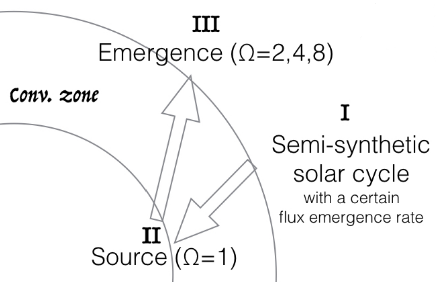
Figure 13: A schematic representation of the mappings between the surface and the base of the convection zone in the model. $\Omega$ denotes the equatorial rotation rate in solar units. The roman numerals refer to the steps of the procedure.

1. Generate a random realisation of the spot group record (SGR) with a certain flux emergence rate $\tilde{s}$ (see Sects. 2.1.1–2.1.2). The mean latitude of this SGR depends on $\tilde{s}$ (Eq. 1).

2. Map the latitudes obtained in step I down to the base of the convection zone, by interpolating the flux tube rise table for the solar rotation rate, $\tilde{\omega}=1$ (Sect. 2.2.2).

3. Take the time series resulting from step II as the base latitudes of the flux tubes leading to spot groups, for a given rotation rate, $\tilde{\omega}$. Generate the emergence latitudes and tilt angles for $\tilde{\omega}$, by interpolating within the flux-tube rise table (Sect. 2.2.2).

4. To simulate the effect of active region nesting, modify the longitudes and latitudes obtained in the previous steps, using a probabilistic approach (Appendix C).

Appendix C Nests of activity

To simulate the observed tendency of flux emergence in the vicinity of recent emergence, we modified the longitudes and latitudes of BMRs in our standard starspot record, using a probabilistic approach. We first set a generic probability $0<p<1$ for each BMR with coordinates $(\lambda,\phi)$ to be part of a nest. In this study, we chose a rather high probability of $p=0.7$ to clearly demonstrate the effects of nesting. This value has made the cycle variation of the equatorial dipole moment much more similar to the observed variations (Wang 2014, see Fig. 3) in comparison to the unnested case.

If a uniformly chosen random number $E_{i}\sim U[0,1]$ is less than $p$, then the coordinates of the $i$th BMR of the unnested record is considered as a potential nest centre, $(\lambda_{c},\phi_{c})_{i}$. If the next random number $E_{i+1}<p$, then the $(i+1)$th BMR belongs to the nest of the $i$th BMR. The coordinates of such a BMR is then given a modified pair of coordinates $(\lambda_{m},\phi_{m})_{i+1}$, which are drawn from a normal distribution centred around $(\lambda_{c},\phi_{c})_{i}$ with widths $2^{\circ}$ in latitude and $3^{\circ}$ in longitude, close to the empirical values obtained by Pojoga & Cudnik (2002) for Cycle 23. The procedure is continued iteratively until for the $(i+k)$th BMR $E_{i+k}\geqslant p$ holds. Such a BMR is considered as an isolated spot group, while its original coordinates are kept unchanged.