Push-Pull Gradient Methods for Distributed Optimization in Networks

Abstract

In this paper, we focus on solving a distributed convex optimization problem in a network, where each agent has its own convex cost function and the goal is to minimize the sum of the agents’ cost functions while obeying the network connectivity structure. In order to minimize the sum of the cost functions, we consider new distributed gradient-based methods where each node maintains two estimates, namely, an estimate of the optimal decision variable and an estimate of the gradient for the average of the agents’ objective functions. From the viewpoint of an agent, the information about the gradients is pushed to the neighbors, while the information about the decision variable is pulled from the neighbors hence giving the name “push-pull gradient methods”. The methods utilize two different graphs for the information exchange among agents, and as such, unify the algorithms with different types of distributed architecture, including decentralized (peer-to-peer), centralized (master-slave), and semi-centralized (leader-follower) architecture. We show that the proposed algorithms and their many variants converge linearly for strongly convex and smooth objective functions over a network (possibly with unidirectional data links) in both synchronous and asynchronous random-gossip settings. In particular, under the random-gossip setting, “push-pull” is the first class of algorithms for distributed optimization over directed graphs. Moreover, we numerically evaluate our proposed algorithms in both scenarios, and show that they outperform other existing linearly convergent schemes, especially for ill-conditioned problems and networks that are not well balanced.

I Introduction

In this paper, we consider a system involving $n$ agents whose goal is to collaboratively solve the following problem:

$$\begin{array}[]{c}\min\limits_{x\in\mathbb{R}^{p}}~{}f(x):=\sum\limits_{i=1}^{n}f_{i}(x),\end{array}$$ (1)

where $x$ is the global decision variable and each function $f_{i}:\mathbb{R}^{p}\rightarrow\mathbb{R}$ is convex and known by agent $i$ only. The agents are embedded in a communication network, and their goal is to obtain an optimal and consensual solution through local neighbor communications and information exchange. This local exchange is desirable in situations where the exchange of a large amount of data is prohibitively expensive due to limited communication resources.

To solve problem (1) in a networked system of $n$ agents, many algorithms have been proposed under various assumptions on the objective functions and on the underlying networks/graphs. Static undirected graphs were extensively considered in the literature [2, 3, 4, 5, 6]. References [7, 8, 9] studied time-varying and/or stochastic undirected networks. Directed graphs were discussed in [10, 11, 12, 9, 13, 14]. Centralized (master-slave) algorithms were discussed in [15], where extensive applications in learning can be found. Parallel, coordinated, and asynchronous algorithms were discussed in [16] and the references therein. The reader is also referred to the recent paper [17] and the references therein for a comprehensive survey on distributed optimization algorithms.

In the first part of this paper, we introduce a novel gradient-based algorithm (Push-Pull) for distributed (consensus-based) optimization in directed graphs. Unlike the push-sum type protocol used in the previous literature [9, 14], our algorithm uses a row stochastic matrix for the mixing of the decision variables, while it employs a column stochastic matrix for tracking the average gradients. Although motivated by a fully decentralized scheme, we show that Push-Pull can work both in fully decentralized networks and in two-tier networks.

Gossip-based communication protocols are popular choices for distributed computation due to their low communication costs [18, 19, 20, 21]. In the second part of this paper, we consider a random-gossip push-pull algorithm (G-Push-Pull) where at each iteration, an agent wakes up uniformly randomly and communicates with one or two of its neighbors. Both Push-Pull and G-Push-Pull have different variants. We show that they all converge linearly to the optimal solution for strongly convex and smooth objective functions.

I-A Related Work

Our emphasis in the literature review is on the decentralized optimization, since our approach builds on a new understanding of the decentralized consensus-based methods for directed communication networks. Most references, including [2, 3, 22, 23, 4, 6, 24, 25, 26, 27, 28, 29], often restrict the underlying network connectivity structure, or more commonly require doubly stochastic mixing matrices. The work in [2] has been the first to demonstrate the linear convergence of an ADMM-based decentralized optimization scheme. Reference [3] uses a gradient difference structure in the algorithm to provide the first-order decentralized optimization algorithm which is capable of achieving the typical convergence rates of a centralized gradient method, while references [22, 23] deal with the second-order decentralized methods. By using Nesterov’s acceleration, reference [4] has obtained a method whose convergence time scales linearly in the number of agents $n$, which is the best scaling with $n$ currently known. More recently, for a class of so-termed dual friendly functions, papers [6, 24] have obtained an optimal decentralized consensus optimization algorithm whose dependency on the condition number of the system’s objective function achieves the best known scaling in the order of $O(\sqrt{\kappa})$. Work in [28, 29] investigates proximal-gradient methods which can tackle (1) with proximal friendly component functions. Paper [30] extends the work in [2] to handle asynchrony and delays. References [31, 32] considered a stochastic variant of problem (1) in asynchronous networks. A tracking technique has been recently employed to develop decentralized algorithms for tracking the average of the Hessian/gradient in second-order methods [23], allowing uncoordinated stepsize [25, 26], handling non-convexity [27], and achieving linear convergence over time-varying graphs [9].

For directed graphs, to eliminate the need of constructing a doubly stochastic matrix in reaching consensus, reference [33] proposes the push-sum protocol. Reference [34] has been the first to propose a push-sum based distributed optimization algorithm for directed graphs. Then, based on the push-sum technique again, a decentralized subgradient method for time-varying directed graphs has been proposed and analyzed in [10]. Aiming to improve convergence for a smooth objective function and a fixed directed graph, the work in [13, 12] modifies the algorithm from [3] with the push-sum technique, thus providing a new algorithm which converges linearly for a strongly convex objective function on a static graph. However, the algorithm requires a careful selection of the stepsize which may be even non-existent in some cases [13]. This stability issue has been resolved in [9] in a more general setting of time-varying directed graphs. The work in [14, 35] considers an algorithm that uses only row-stochastic mixing matrices and still achieves linear convergence over fixed directed graphs.

Simultaneously and independently, a paper [36] has proposed an algorithm that is similar to the synchronous variant proposed in this paper. By contrast, the work in [36] does not show that the algorithm unifies different architectures. Moreover, asynchronous or time-varying cases were not discussed either therein.

I-B Main Contribution

The main contribution of this paper is threefold. First, we design new distributed optimization methods (Push-Pull and G-Push-Pull) and their many variants for directed graphs. These methods utilize two different graphs for the information exchange among agents, and as such, unify different computation and communication architectures, including decentralized (peer-to-peer), centralized (master-slave), and semi-centralized (leader-follower) architecture. To the best of our knowledge, these are the first algorithms in the literature that enjoy such property.

Second, we establish the linear convergence of the proposed methods in both synchronous (Push-Pull) and asynchronous random-gossip (G-Push-Pull) settings. In particular, G-Push-Pull is the first class of gossip-type algorithms for distributed optimization over directed graphs.

Finally, in our proposed methods each agent in the network is allowed to use a different nonnegative stepsize, and only one of such stepsizes needs to be positive. This is a unique feature compared to the existing literature (e.g., [9, 14]).

Some of the results related to a variant of Push-Pull will appear in Proceedings of the 57th IEEE Conference on Decision and Control [1]. In contrast, the current work analyzes a different, more communication-efficient variant of Push-Pull, adopts an uncoordinated stepsize policy which generalizes the scheme in [1], and introduces G-Push-Pull in extra. It also contains detailed proofs omitted from the conference version.

I-C Organization of the Paper

The structure of this paper is as follows. We first provide notation and state basic assumptions in Subsection I-D. Then we introduce the push-pull gradient method in Section II along with the intuition of its design and some examples explaining how it relates to (semi-)centralized and decentralized optimization. We establish the linear convergence of the push-pull algorithm in Section III. In Section IV we introduce the random-gossip push-pull method (G-Push-Pull) and demonstrate its linear convergence in Section V. In Section VI we conduct numerical experiments to verify our theoretical claims. Concluding remarks are given in Section VII.

I-D Notation and Assumption

Throughout the paper, vectors default to columns if not otherwise specified. Let $\mathcal{N}=\{1,2,\ldots,n\}$ be the set of agents. Each agent $i\in\mathcal{N}$ holds a local copy $x_{i}\in\mathbb{R}^{p}$ of the decision variable and an auxiliary variable $y_{i}\in\mathbb{R}^{p}$ tracking the average gradients, where their values at iteration $k$ are denoted by $x_{i,k}$ and $y_{i,k}$, respectively. Let

$$\mathbf{x}:=[x_{1},x_{2},\ldots,x_{n}]^{\intercal}\in\mathbb{R}^{n\times p},$$

$$\mathbf{y}:=[y_{1},y_{2},\ldots,y_{n}]^{\intercal}\in\mathbb{R}^{n\times p}.$$

Define $F(\mathbf{x})$ to be an aggregate objective function of the local variables, i.e., $F(\mathbf{x}):=\sum_{i=1}^{n}f_{i}(x_{i})$, and write

$$\nabla F(\mathbf{x}):=\left[\nabla f_{1}(x_{1})^{\intercal},\nabla f_{2}(x_{2})^{\intercal},\ldots,\nabla f_{n}(x_{n})^{\intercal}\right]\in\mathbb{R}^{n\times p}.$$

We use the symbol $\mathbf{tr}\{\cdot\}$ to denote the trace of a square matrix.

Definition 1.

Given an arbitrary vector norm $\|\cdot\|$ on $\mathbb{R}^{n}$, for any $\mathbf{x}\in\mathbb{R}^{n\times p}$, we define

$$\|\mathbf{x}\|:=\left\|\left[\|\mathbf{x}^{(1)}\|,\|\mathbf{x}^{(2)}\|,\ldots,\|\mathbf{x}^{(p)}\|\right]\right\|_{2},$$

where $\mathbf{x}^{(1)},\mathbf{x}^{(2)},\ldots,\mathbf{x}^{(p)}\in\mathbb{R}^{n}$ are columns of $\mathbf{x}$, and $\|\cdot\|_{2}$ represents the $2$-norm.

We make the following assumption on the functions $f_{i}$ in (1).

Assumption 1.

Each $f_{i}$ is $\mu$-strongly convex and its gradient is $L$-Lipschitz continuous, i.e., for any $x,x^{\prime}\in\mathbb{R}^{p}$,

$$\begin{split}&\langle\nabla f_{i}(x)-\nabla f_{i}(x^{\prime}),x-x^{\prime}\rangle\geq\mu\|x-x^{\prime}\|_{2}^{2},\\ &\|\nabla f_{i}(x)-\nabla f_{i}(x^{\prime})\|_{2}\leq L\|x-x^{\prime}\|_{2}.\end{split}$$

Under Assumption 1, there exists a unique optimal solution $x^{*}\in\mathbb{R}^{p}$ to problem (1).

We use directed graphs to model the interaction topology among agents. A directed graph (digraph) is a pair $\mathcal{G}=(\mathcal{N},\mathcal{E})$, where $\mathcal{N}$ is the set of vertices (nodes) and the edge set $\mathcal{E}\subseteq\mathcal{N}\times\mathcal{N}$ consists of ordered pairs of vertices. If there is a directed edge from node $i$ to node $j$ in $\mathcal{G}$, or $(i,j)\in\mathcal{E}$, then $i$ is defined as the parent node and $j$ is defined as the child node. Information can be transmitted from the parent node to the child node directly. A directed path in graph $\mathcal{G}$ is a sequence of edges $(i,j)$, $(j,k)$, $(k,l)\ldots$. Graph $\mathcal{G}$ is called strongly connected if there is a directed path between any pair of distinct vertices. A directed tree is a digraph where every vertex, except for the root, has only one parent. A spanning tree of a digraph is a directed tree that connects the root to all other vertices in the graph. A subgraph $\mathcal{S}$ of graph $\mathcal{G}$ is a graph whose set of vertices and set of edges are all subsets of $\mathcal{G}$ (see [37]).

Given a nonnegative matrix $\mathbf{M}=[m_{ij}]\in\mathbb{R}^{n\times n}$, the digraph induced by the matrix $\mathbf{M}$ is denoted by $\mathcal{G}_{\mathbf{M}}=(\mathcal{N},\mathcal{E}_{\mathbf{M}})$, where $\mathcal{N}=\{1,2,\ldots,n\}$ and $(j,i)\in\mathcal{E}_{\mathbf{M}}$ iff (if and only if) $m_{ij}>0$. We let $\mathcal{R}_{\mathbf{M}}$ be the set of roots of all possible spanning trees in the graph $\mathcal{G}_{\mathbf{M}}$. For an arbitrary agent $i\in\mathcal{N}$, we define its in-neighbor set $\mathcal{N}^{\mathrm{in}}_{\mathbf{M},i}$ as the collection of all individual agents that $i$ can actively and reliably pull data from; we also define its out-neighbor set $\mathcal{N}^{\mathrm{out}}_{\mathbf{M},i}$ as the collection of all individual agents that can passively and reliably receive data from $i$. In the situation when the set is time-varying, we further add a subscript to indicate it generates a sequence of sets. For example, $\mathcal{N}^{\mathrm{in}}_{\mathbf{M},i,k}$ is the in-neighbor set of $i$ at time/iteration $k$.

II A Push-Pull Gradient Method

To proceed, we first illustrate and highlight the proposed algorithm, which we call Push-Pull in the following (Algorithm 1).

Algorithm 1: Push-Pull

Each agent $i$ chooses its local step size $\alpha_{i}\geq 0$,

in-bound mixing/pulling weights $R_{ij}\geq 0$ for all $j\in\mathcal{N}^{\mathrm{in}}_{\mathbf{R},i}$,

and out-bound pushing weights $C_{li}\geq 0$ for all $l\in\mathcal{N}^{\mathrm{out}}_{\mathbf{C},i}$;

Each agent $i$ initializes with any arbitrary $x_{i,0}\in\mathbb{R}^{p}$ and $y_{i,0}=\nabla f_{i}(x_{i,0})$;

for $k=0,1,\cdots$, do

for each $i\in\mathcal{N}$,

agent $i$ pulls $(x_{j,k}-\alpha_{j}y_{j,k})$ from each $j\in\mathcal{N}^{\mathrm{in}}_{\mathbf{R},i}$;

agent $i$ pushes $C_{li}y_{i,k}$ to each $l\in\mathcal{N}^{\mathrm{out}}_{\mathbf{C},i}$;

for each $i\in\mathcal{N}$,

$x_{i,k+1}=\sum_{j=1}^{n}R_{ij}(x_{j,k}-\alpha_{j}y_{j,k})$;

$y_{i,k+1}=\sum_{j=1}^{n}C_{ij}y_{j,k}+\nabla f_{i}(x_{i,k+1})-\nabla f_{i}(x_{i,k})$;

end for

Algorithm 1 (Push-Pull) can be rewritten in the following aggregated form:

$$\mathbf{x}_{k+1}=\mathbf{R}(\mathbf{x}_{k}-\boldsymbol{\alpha}\mathbf{y}_{k}),$$ (2a)

$$\mathbf{y}_{k+1}=\mathbf{C}\mathbf{y}_{k}+\nabla F(\mathbf{x}_{k+1})-\nabla F(\mathbf{x}_{k}),$$ (2b)

where $\boldsymbol{\alpha}=\text{diag}\{\alpha_{1},\alpha_{2},\ldots,\alpha_{n}\}$ is a nonnegative diagonal matrix and $\mathbf{R}=[R_{ij}],\,\mathbf{C}=[C_{ij}]\in\mathbb{R}^{n\times n}$. We make the following assumption on the matrices $\mathbf{R}$ and $\mathbf{C}$.

Assumption 2.

The matrix $\mathbf{R}\in\mathbb{R}^{n\times n}$ is nonnegative row-stochastic and $\mathbf{C}\in\mathbb{R}^{n\times n}$ is nonnegative column-stochastic, i.e., $\mathbf{R}\mathbf{1}=\mathbf{1}$ and $\mathbf{1}^{\intercal}\mathbf{C}=\mathbf{1}^{\intercal}$. In addition, the diagonal entries of $\mathbf{R}$ and $\mathbf{C}$ are positive, i.e., $R_{ii}>0$ and $C_{ii}>0$ for all $i\in\mathcal{N}$.

As a result of $\mathbf{C}$ being column-stochastic, we have by induction that

$$\frac{1}{n}\mathbf{1}^{\intercal}\mathbf{y}_{k}=\frac{1}{n}\mathbf{1}^{\intercal}\nabla F(\mathbf{x}_{k}),\qquad\forall k.$$ (3)

Relation (3) is critical for (a subset of) the agents to track the average gradient $\mathbf{1}^{\intercal}\nabla F(\mathbf{x}_{k})/n$ through the $\mathbf{y}$-update.

Remark 1.

At each iteration, each agent will “push” information about gradients to its out-neighbors and “pull” the decision variables from its in-neighbors, respectively. Each component of $\mathbf{y}_{k}$ plays the role of tracking the average gradient using the column-stochastic matrix $\mathbf{C}$ while each component of $\mathbf{x}_{k}$ performs optimization seeking by average consensus using a row-stochastic matrix $\mathbf{R}$. The structure of Algorithm 1 resembles that of the gradient tracking methods as in [9, 25] with the doubly stochastic matrix being split into a row-stochastic matrix and a column-stochastic matrix. Such an asymmetric $\mathbf{R}$-$\mathbf{C}$ structure has already been used in the literature for achieving average consensus [38]. However, the proposed optimization algorithm can not be interpreted as a linear system since it introduces nonlinear dynamics due to the gradient terms.

We now give the condition on the structures of graphs $\mathcal{G}_{\mathbf{R}}$ and $\mathcal{G}_{\mathbf{C}^{\intercal}}$ induced by matrices $\mathbf{R}$ and $\mathbf{C}^{\intercal}$, respectively. Note that $\mathcal{G}_{\mathbf{C}^{\intercal}}$ is identical to the graph $\mathcal{G}_{\mathbf{C}}$ with all its edges reversed.

Assumption 3.

The graphs $\mathcal{G}_{\mathbf{R}}$ and $\mathcal{G}_{\mathbf{C}^{\intercal}}$ each contain at least one spanning tree. Moreover, there exists at least one node that is a root of spanning trees for both $\mathcal{G}_{\mathbf{R}}$ and $\mathcal{G}_{\mathbf{C}^{\intercal}}$, i.e., $\mathcal{R}_{\mathbf{R}}\cap\mathcal{R}_{\mathbf{C}^{\intercal}}\neq\emptyset$, where $\mathcal{R}_{\mathbf{R}}$ (resp., $\mathcal{R}_{\mathbf{C}^{\intercal}}$) is the set of roots of all possible spanning trees in the graph $\mathcal{G}_{\mathbf{R}}$ (resp., $\mathcal{G}_{\mathbf{C}^{\intercal}}$).

Assumption 3 is weaker than requiring that both $\mathcal{G}_{\mathbf{R}}$ and $\mathcal{G}_{\mathbf{C}}$ are strongly connected, which was assumed in most previous works (e.g., [9, 14, 36]). This relaxation offers us more flexibility in designing graphs $\mathcal{G}_{\mathbf{R}}$ and $\mathcal{G}_{\mathbf{C}}$. For instance, suppose that we have a strongly connected communication graph $\mathcal{G}$. Then there are multiple ways to construct $\mathcal{G}_{\mathbf{R}}$ and $\mathcal{G}_{\mathbf{C}}$ satisfying Assumption 3. One trivial approach is to set $\mathcal{G}_{\mathbf{R}}=\mathcal{G}_{\mathbf{C}}=\mathcal{G}$. Another way is to pick at random $i_{r}\in\mathcal{N}$ and let $\mathcal{G}_{\mathbf{R}}$ (resp., $\mathcal{G}_{\mathbf{C}}$) be a spanning tree (resp., reversed spanning tree) contained in $\mathcal{G}$ with $i_{r}$ as its root. Once graphs $\mathcal{G}_{\mathbf{R}}$ and $\mathcal{G}_{\mathbf{C}}$ are established, matrices $\mathbf{R}$ and $\mathbf{C}$ can be designed accordingly.

Remark 2.

There are different ways to design the weights in $\mathbf{R}$ and $\mathbf{C}$ by each agent locally. For example, each agent $i$ may choose $R_{ij}=\frac{1}{|\mathcal{N}^{\mathrm{in}}_{\mathbf{R},i}|+c_{R}}$ for some constant $c_{R}>0$ for all $j\in\mathcal{N}^{\mathrm{in}}_{\mathbf{R},i}$ and let $R_{ii}=1-\sum_{j\in\mathcal{N}^{\mathrm{in}}_{\mathbf{R},i}}$. Similarly, agent $i$ can choose $C_{li}=\frac{1}{|\mathcal{N}^{\mathrm{out}}_{\mathbf{C},i}|+c_{C}}$ for some constant $c_{C}>0$ for all $l\in\mathcal{N}^{\mathrm{out}}_{\mathbf{C},i}$ and let $C_{ii}=1-\sum_{l\in\mathcal{N}^{\mathrm{out}}_{\mathbf{C},i}}$. Such a choice of mixing weights will render $\mathbf{R}$ row-stochastic and $\mathbf{C}$ column-stochastic, thus satisfying Assumption 2.

We have the following result from Assumption 2 and Assumption 3.

Lemma 1.

Under Assumption 2 and Assumption 3, the matrix $\mathbf{R}$ has a unique nonnegative left eigenvector $u^{\intercal}$ (w.r.t. eigenvalue $1$) with $u^{\intercal}\mathbf{1}=n$, and the matrix $\mathbf{C}$ has a unique nonnegative right eigenvector $v$ (w.r.t. eigenvalue $1$) with $\mathbf{1}^{\intercal}v=n$ (see [39]). Moreover, eigenvector $u^{\intercal}$ (resp., $v$) is nonzero only on the entries associated with agents $i\in\mathcal{R}_{\mathbf{R}}$ (resp., $j\in\mathcal{R}_{\mathbf{C}^{\intercal}}$), and $u^{\intercal}v>0$.

Proof.

See Appendix A-A. ∎

Finally, we assume the following condition regarding the step sizes $\{\alpha_{i}\}$.

Assumption 4.

There is at least one agent $i\in\mathcal{R}_{\mathbf{R}}\cap\mathcal{R}_{\mathbf{C}^{\intercal}}$ whose step size $\alpha_{i}$ is positive.

Assumption 3 and Assumption 4 hint on the crucial role of the set $\mathcal{R}_{\mathbf{R}}\cap\mathcal{R}_{\mathbf{C}^{\intercal}}$. In what follows, we provide some intuition for the development of Push-Pull and an interpretation of the algorithm from another perspective. The discussions will shed light on the rationale behind the assumptions.

To motivate the development of Push-Pull, let us consider the optimality condition for (1) in the following form:

$$\mathbf{x}^{*}\in\mathrm{null}\{\mathbf{I}-\mathbf{R}\},$$ (4a)

$$\mathbf{1}^{\intercal}\nabla F(\mathbf{x}^{*})=0,$$ (4b)

where $\mathbf{x}^{*}:=\mathbf{1}{x^{*}}^{\intercal}$ and $\mathbf{R}$ satisfies Assumption 2. Consider the algorithm in (2). Suppose that the algorithm produces two sequences $\{\mathbf{x}_{k}\}$ and $\{\mathbf{y}_{k}\}$ converging to some points $\mathbf{x}_{\infty}$ and $\mathbf{y}_{\infty}$, respectively. Then from (2a) and (2b) we would have

$$(\mathbf{I}-\mathbf{R})(\mathbf{x}_{\infty}-\boldsymbol{\alpha}\mathbf{y}_{\infty})+\boldsymbol{\alpha}\mathbf{y}_{\infty}=0,$$ (5a)

$$(\mathbf{I}-\mathbf{C})\mathbf{y}_{\infty}=0.$$ (5b)

If $\mathrm{span}\{\mathbf{I}-\mathbf{R}\}$ and $\boldsymbol{\alpha}\cdot\mathrm{null}\{\mathbf{I}-\mathbf{C}\}$ are disjoint, from (5) we would have $\mathbf{x}_{\infty}\in\mathrm{null}\{\mathbf{I}-\mathbf{R}\}$ and $\boldsymbol{\alpha}\mathbf{y}_{\infty}=\mathbf{0}$. Hence $\mathbf{x}_{\infty}$ satisfies the optimality condition in (4a). In light of (5b), Assumption 4, and Lemma 1, we have $\mathbf{y}_{\infty}\in\mathrm{null}\{\boldsymbol{\alpha}\}\cap\mathrm{null}\{\mathbf{I}-\mathbf{C}\}=\{\mathbf{0}\}$. Then from (3) we know that $\mathbf{1}^{\intercal}\nabla F(\mathbf{x}_{\infty})=\mathbf{1}^{\intercal}\mathbf{y}_{\infty}=\mathbf{0}$, which is exactly the optimality condition in (4b).

For another interpretation of Push-Pull, notice that under Assumptions 2 and 3, with linear rates of convergence,

$$\lim_{k\rightarrow\infty}\mathbf{R}^{k}=\frac{\mathbf{1}u^{\intercal}}{n},\ \ \lim_{k\rightarrow\infty}\mathbf{C}^{k}=\frac{v\mathbf{1}^{\intercal}}{n}.$$ (6)

Thus with comparatively small step sizes, relation (6) together with (3) implies that $\mathbf{x}_{k}\simeq\mathbf{1}u^{\intercal}\mathbf{x}_{k-K}/n$ (for some fixed $K>0$) and $\mathbf{y}_{k}\simeq v\mathbf{1}^{\intercal}\nabla F(\mathbf{x}_{k})/n$. From the proof of Lemma 1, eigenvector $u$ (resp., $v$) is nonzero only on the entries associated with agents $i\in\mathcal{R}_{\mathbf{R}}$ (resp., $j\in\mathcal{R}_{\mathbf{C}^{\intercal}}$). Hence $\mathbf{x}_{k}\simeq\mathbf{1}u^{\intercal}\mathbf{x}_{k-K}/n$ indicates that only the state information of agents $i\in\mathcal{R}_{\mathbf{R}}$ are pulled by the entire network, and $\mathbf{y}_{k}\simeq v\mathbf{1}^{\intercal}\nabla F(\mathbf{x}_{k})/n$ implies that only agents $j\in\mathcal{R}_{\mathbf{C}^{\intercal}}$ are pushed and tracking the average gradients. This “push” and “pull” information structure gives the name of the algorithm. The assumption $\mathcal{R}_{\mathbf{R}}\cap\mathcal{R}_{\mathbf{C}^{\intercal}}\neq\emptyset$ essentially says at least one agent needs to be both “pulled” and “pushed”.

The above discussion has mathematically interpreted why the use of row stochastic matrices and column stochastic matrices is reasonable. Now let us explain from the implementation aspect why Algorithm 1 is called “Push-Pull” and why it is more feasible to be implemented with “Push” and “Pull” at the same time. When the information across agents need to be diffused/fused, either an agent needs to know what scaling weights it needs to put on the quantities sending out to other agents, or it needs to know how to combine the quantities coming in with correct weights. In particular, we have the following specific weight assignment strategies:

• For the networked system to maintain $\sum_{l}C_{li}=1$, an apparently convenient way is to let agent $i$ scale its data by $C_{li},\forall l$, before sending/pushing out messages. In this way, it becomes agent $i$’s responsibility to synchronize out-neighbors’ receptions of messages and it is natural to employ a reliable push-communication-protocol to implement such operations.

• Unlike what happens in A), to maintain $\sum_{j}R_{ij}=1$, the only seemingly feasible way is to let the receiver $i$ perform the tasks of scaling and combination/addition since it would be difficult for the sender to know the weights or adjust the weights accordingly, especially when the network changes. Thus, it is natural to employ a pull-communication-protocol for the above operations.

II-A Unifying Different Distributed Computational Architecture

We now demonstrate how the proposed algorithm (2) unifies different types of distributed architecture, including decentralized, centralized, and semi-centralized architecture. For the fully decentralized case, suppose we have a graph $\mathcal{G}$ that is undirected and connected. Then we can set $\mathcal{G}_{\mathbf{R}}=\mathcal{G}_{\mathbf{C}}=\mathcal{G}$ and let $\mathbf{R}=\mathbf{C}$ be symmetric matrices, in which case the proposed algorithm degrades to the one considered in [9, 25]; if the graph is directed and strongly connected, we can also let $\mathcal{G}_{\mathbf{R}}=\mathcal{G}_{\mathbf{C}}=\mathcal{G}$ and design the weights for $\mathbf{R}$ and $\mathbf{C}$ correspondingly.

To illustrate the less straightforward situation of (semi)-centralized networks, let us give a simple example. Consider a four-node star network composed by $\{1,2,3,4\}$ where node $1$ is situated at the center and nodes $2$, $3$, and $4$ are (bidirectionally) connected with node $1$ but not connected to each other. In this case, the matrix $\mathbf{R}$ in our algorithm can be chosen as

$$\mathbf{R}=\left[\begin{array}[]{cccc}1&0&0&0\cr 0.5&0.5&0&0\cr 0.5&0&0.5&0\cr 0.5&0&0&0.5\end{array}\right],\ \ \mathbf{C}=\left[\begin{array}[]{cccc}1&0.5&0.5&0.5\cr 0&0.5&0&0\cr 0&0&0.5&0\cr 0&0&0&0.5\end{array}\right].$$

For a graphical illustration, the corresponding network topologies of $\mathcal{G}_{\mathbf{R}}$ and $\mathcal{G}_{\mathbf{C}}$ are shown in Fig. 1.

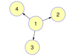
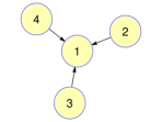
Figure 1: On the left is the graph $\mathcal{G}_{\mathbf{R}}$ and on the right is the graph $\mathcal{G}_{\mathbf{C}}$.

The central node $1$’s information regarding $x_{1,k}$ is pulled by the neighbors (the entire network in this case) through $\mathcal{G}_{\mathbf{R}}$; the others only passively infuse the information from node $1$. At the same time, node $1$ has been pushed information regarding $y_{i,k}$ ($i=2,3,4$) from the neighbors through $\mathcal{G}_{\mathbf{C}}$; the other nodes only actively comply with the request from node $1$. This motivates the algorithm’s name push-pull gradient method. Although nodes $2$, $3$, and $4$ are updating their $y_{i}$’s accordingly, these quantities do not have to contribute to the optimization procedure and will die out geometrically fast due to the weights in the last three rows of $\mathbf{C}$. Consequently, in this special case, the local stepsize $\alpha$ for agents $2$, $3$, and $4$ can be set to $0$. Without loss of generality, suppose $f_{1}(x)=0,\forall x$. Then the algorithm becomes a typical centralized algorithm for minimizing $\sum_{i=2}^{4}f_{i}(x)$ where the master node $1$ utilizes the slave nodes $2$, $3$, and $4$ to compute the gradient information in a distributed way.

Taking the above as an example for explaining the semi-centralized case, it is worth noting that node $1$ can be replaced by a strongly connected subnet in $\mathcal{G}_{\mathbf{R}}$ and $\mathcal{G}_{\mathbf{C}}$, respectively. Correspondingly, nodes $2$, $3$, and $4$ can all be replaced by subnets as long as the information from the master layer in these subnets can be diffused to all the slave layer agents in $\mathcal{G}_{\mathbf{R}}$, while the information from all the slave layer agents can be diffused to the master layer in $\mathcal{G}_{\mathbf{C}}$. Specific requirements on connectivities of slave subnets can be understood by using the concept of rooted trees. We refer to the nodes as leaders if their roles in the network are similar to the role of node $1$; and the other nodes are termed as followers. Note that after the replacement of the individual nodes by subnets, the network structure in all subnets are decentralized, while the relationship between leader subnet and follower subnets is master-slave. This is why we refer to such an architecture as semi-centralized.

Remark 3 (A class of Push-Pull algorithms).

There can be multiple variants of the proposed algorithm depending on whether the Adapt-then-Combine (ATC) strategy [40] is used in the $\mathbf{x}$-update and/or the $\mathbf{y}$-update (see Remark 3 in [9] for more details). For readability, we only illustrate one algorithm in Algorithm 1 and call it Push-Pull in the above. We also generally use “Push-Pull” to refer to a class of algorithms regardless whether the ATC structure is used, if not causing confusion. Our forthcoming analysis can be adapted to these variants. Our numerical tests in Section VI only involve some variants.

III Convergence Analysis for Push-Pull

In this section, we study the convergence properties of the proposed algorithm. We first define the following variables:

$$\bar{x}_{k}:=\frac{1}{n}u^{\intercal}\mathbf{x}_{k},\qquad\bar{y}_{k}:=\frac{1}{n}\mathbf{1}^{\intercal}\mathbf{y}_{k}.$$

Our strategy is to bound $\|\bar{x}_{k+1}-x^{*}\|_{2}$, $\|\mathbf{x}_{k+1}-\mathbf{1}\bar{x}_{k+1}\|_{\mathrm{R}}$ and $\|\mathbf{y}_{k+1}-v\bar{y}_{k+1}\|_{\mathrm{C}}$ in terms of linear combinations of their previous values, where $\|\cdot\|_{\mathrm{R}}$ and $\|\cdot\|_{\mathrm{C}}$ are specific norms to be defined later. In this way we establish a linear system of inequalities which allows us to derive the convergence results. The proof technique was inspired by [5, 14].

Before diving into the detailed analysis, we present the main convergence result for the Push-Pull algorithm in (2) in the following theorem.

Theorem 1.

Suppose Assumptions 1-3 hold, $\alpha^{\prime}\geq M\hat{\alpha}$ for some $M>0$ and

$$\hat{\alpha}\leq\min\left\{\frac{2c_{3}}{c_{2}+\sqrt{c_{2}^{2}+4c_{1}c_{3}}},\frac{(1-\sigma_{\mathrm{C}})}{2\sigma_{\mathrm{C}}\delta_{\mathrm{C},2}\|\mathbf{R}\|_{2}L}\right\},$$ (7)

where $c_{1},c_{2},c_{3}$ are given in (34)-(41), and $\sigma_{\mathrm{C}}$ and $\delta_{\mathrm{C},2}$ are defined in Lemma 4 and Lemma 6, respectively. Then, the quantities $\|\bar{x}_{k}-x^{*}\|_{2}$, $\|\mathbf{x}_{k}-\mathbf{1}\bar{x}_{k}\|_{\mathrm{R}}$ and $\|\mathbf{y}_{k}-v\bar{y}_{k}\|_{\mathrm{C}}$ all converge to $0$ at the linear rate $\mathcal{O}(\rho(\mathbf{A})^{k})$ with $\rho(\mathbf{A})<1$, where $\rho(\mathbf{A})$ denotes the spectral radius of the matrix $\mathbf{A}$ defined in (18).

Remark 4.

Note that

$$\alpha^{\prime}=\frac{1}{n}u^{\intercal}\boldsymbol{\alpha}v=\sum_{i\in\mathcal{R}_{\mathbf{R}}\cap\mathcal{R}_{\mathbf{C}^{\intercal}}}\frac{1}{n}u_{i}v_{i}\alpha_{i}.$$

The condition $\alpha^{\prime}\geq M\hat{\alpha}$ is automatically satisfied for a fixed $M$ in various situations. For example, if $\max_{i\in\mathcal{N}}\alpha_{i}=\max_{i\in\mathcal{R}_{\mathbf{R}}\cap\mathcal{R}_{\mathbf{C}^{\intercal}}}\alpha_{i}$ (which is always true when both $\mathcal{G}_{\mathbf{R}}$ and $\mathcal{G}_{\mathbf{C}^{\intercal}}$ are strongly connected), we can take $M=u_{j}v_{j}/n$ for $j=\arg\max_{i\in\mathcal{R}_{\mathbf{R}}\cap\mathcal{R}_{\mathbf{C}^{\intercal}}}\alpha_{i}$. For another example, if all $\alpha_{i}$ are equal, then $M=u^{\intercal}v/n$.

In general, the constant $M$ roughly measures the ratio of stepsizes used by agents in $\mathcal{R}_{\mathbf{R}}\cap\mathcal{R}_{\mathbf{C}^{\intercal}}$ and by all the agents. According to condition (7) and definitions (34)-(41), smaller $M$ leads to a tighter upper bound on the maximum stepsize $\hat{\alpha}$.

Remark 5.

The upperbound on the stepsizes can be exactly calculated by (7) assuming the weight matrices $\mathbf{R}$ and $\mathbf{C}$ are known. Note that since our proof technique is similar to those using the small-gain theorem (see e.g., [5, 9]), the upperbound obtained here may be conservative. Thus, it is still open how to develop new analytical tools to derive a tighter upperbound. However, it is worth mentioning that, in our numerical simulations, Push-Pull always allows for a very large region of stepsize choice compared to other distributed optimization algorithms applicable to directed graphs.

Remark 6.

When $\hat{\alpha}$ is sufficiently small, it can be shown that $\rho(\mathbf{A})\simeq 1-\alpha^{\prime}\mu$, in which case the Push-Pull algorithm is comparable to the centralized gradient descent method with stepsize $\alpha^{\prime}$. Since $\alpha^{\prime}=\sum_{i\in\mathcal{R}_{\mathbf{R}}\cap\mathcal{R}_{\mathbf{C}^{\intercal}}}\frac{1}{n}u_{i}v_{i}\alpha_{i}$, only the stepsizes of agents $i\in\mathcal{R}_{\mathbf{R}}\cap\mathcal{R}_{\mathbf{C}^{\intercal}}$ contribute to the convergence speed of Push-Pull. This corresponds to our discussion in Section II-A.

III-A Preliminary Analysis

From the algorithm (2) and Lemma 1, we have

$$\bar{x}_{k+1}=\frac{1}{n}u^{\intercal}\mathbf{R}(\mathbf{x}_{k}-\boldsymbol{\alpha}\mathbf{y}_{k})=\bar{x}_{k}-\frac{1}{n}u^{\intercal}\boldsymbol{\alpha}\mathbf{y}_{k},$$ (8)

and

$$\bar{y}_{k+1}=\frac{1}{n}\mathbf{1}^{\intercal}\left(\mathbf{C}\mathbf{y}_{k}+\nabla F(\mathbf{x}_{k+1})-\nabla F(\mathbf{x}_{k})\right)\\ =\bar{y}_{k}+\frac{1}{n}\mathbf{1}^{\intercal}\left(\nabla F(\mathbf{x}_{k+1})-\nabla F(\mathbf{x}_{k})\right).$$ (9)

Let us further define $g_{k}:=\frac{1}{n}\mathbf{1}^{\intercal}\nabla F(\mathbf{1}\bar{x}_{k})$. Then, we obtain from relation (8) that

$$\bar{x}_{k+1} =\bar{x}_{k}-\frac{1}{n}u^{\intercal}\boldsymbol{\alpha}\left(\mathbf{y}_{k}-v\bar{y}_{k}+v\bar{y}_{k}\right)$$

$$=\bar{x}_{k}-\frac{1}{n}u^{\intercal}\boldsymbol{\alpha}v\bar{y}_{k}-\frac{1}{n}u^{\intercal}\boldsymbol{\alpha}\left(\mathbf{y}_{k}-v\bar{y}_{k}\right)$$

$$=\bar{x}_{k}-\alpha^{\prime}g_{k}-\alpha^{\prime}(\bar{y}_{k}-g_{k})-\frac{1}{n}u^{\intercal}\boldsymbol{\alpha}\left(\mathbf{y}_{k}-v\bar{y}_{k}\right),$$ (10)

where

$$\alpha^{\prime}:=\frac{1}{n}u^{\intercal}\boldsymbol{\alpha}v.$$ (11)

We will show later that Assumptions 3 and 4 ensures $\alpha^{\prime}>0$.

In view of (2) and Lemma 1, using (8) we have

$$\mathbf{x}_{k+1}-\mathbf{1}\bar{x}_{k+1}=\mathbf{R}(\mathbf{x}_{k}-\boldsymbol{\alpha}\mathbf{y}_{k})-\mathbf{1}\bar{x}_{k}+\frac{1}{n}\mathbf{1}u^{\intercal}\boldsymbol{\alpha}\mathbf{y}_{k}\\ =\mathbf{R}(\mathbf{x}_{k}-\mathbf{1}\bar{x}_{k})-\left(\mathbf{R}-\frac{\mathbf{1}u^{\intercal}}{n}\right)\boldsymbol{\alpha}\mathbf{y}_{k}\\ =\left(\mathbf{R}-\frac{\mathbf{1}u^{\intercal}}{n}\right)(\mathbf{x}_{k}-\mathbf{1}\bar{x}_{k})-\left(\mathbf{R}-\frac{\mathbf{1}u^{\intercal}}{n}\right)\boldsymbol{\alpha}\mathbf{y}_{k},$$ (12)

and from (9) we obtain

$$\mathbf{y}_{k+1}-v\bar{y}_{k+1}=\mathbf{C}\mathbf{y}_{k}-v\bar{y}_{k}\\ +\left(\mathbf{I}-\frac{v\mathbf{1}^{\intercal}}{n}\right)\left(\nabla F(\mathbf{x}_{k+1})-\nabla F(\mathbf{x}_{k})\right)\\ =\left(\mathbf{C}-\frac{v\mathbf{1}^{\intercal}}{n}\right)(\mathbf{y}_{k}-v\bar{y}_{k})\\ +\left(\mathbf{I}-\frac{v\mathbf{1}^{\intercal}}{n}\right)\left(\nabla F(\mathbf{x}_{k+1})-\nabla F(\mathbf{x}_{k})\right).$$ (13)

III-B Supporting Lemmas

Before proceeding to prove the main result in Theorem 1, we state a few useful lemmas.

Lemma 2.

Under Assumption 1, there holds

$$\|\bar{y}_{k}-g_{k}\|_{2}\leq\frac{L}{\sqrt{n}}\|\mathbf{x}_{k}-\mathbf{1}\bar{x}_{k}\|_{2},\qquad\|g_{k}\|_{2}\leq L\|\bar{x}_{k}-x^{*}\|_{2}.$$

In addition, when $\alpha^{\prime}\leq 2/(\mu+L)$, we have

$$\|\bar{x}_{k}-\alpha^{\prime}g_{k}-x^{*}\|_{2}\leq(1-\alpha^{\prime}\mu)\|\bar{x}_{k}-x^{*}\|_{2},\qquad\forall k.$$

Proof.

See Appendix A-B. ∎

Lemma 3.

Suppose Assumptions 2-3 hold. Let $\rho_{\mathbf{R}}$ and $\rho_{\mathbf{C}}$ be the spectral radii of $(\mathbf{R}-\mathbf{1}u^{\intercal}/n)$ and $(\mathbf{C}-v\mathbf{1}^{\intercal}/n)$, respectively. Then, we have $\rho_{\mathbf{R}}<1$ and $\rho_{\mathbf{C}}<1$.

Proof.

See Appendix A-C. ∎

Lemma 4.

There exist matrix norms $\|\cdot\|_{\mathrm{R}}$ and $\|\cdot\|_{\mathrm{C}}$ such that $\sigma_{\mathrm{R}}:=\|\mathbf{R}-\frac{\mathbf{1}u^{\intercal}}{n}\|_{\mathrm{R}}<1$, $\sigma_{\mathrm{C}}:=\|\mathbf{C}-\frac{v\mathbf{1}^{\intercal}}{n}\|_{\mathrm{C}}<1$, and $\sigma_{\mathrm{R}}$ and $\sigma_{\mathrm{C}}$ are arbitrarily close to $\rho_{\mathbf{R}}$ and $\rho_{\mathbf{C}}$, respectively. In addition, given any diagonal matrix $\mathbf{W}\in\mathbb{R}^{n\times n}$, we have $\|\mathbf{W}\|_{\mathrm{R}}=\|\mathbf{W}\|_{\mathrm{C}}=\|\mathbf{W}\|_{2}$.

Proof.

See [39, Lemma 5.6.10] and the discussions thereafter. ∎

In the rest of this paper, with a slight abuse of notation, we do not distinguish between the vector norms on $\mathbb{R}^{n}$ and their induced matrix norms.

Lemma 5.

Given an arbitrary norm $\|\cdot\|$, for any $\mathbf{W}\in\mathbb{R}^{n\times n}$ and $\mathbf{x}\in\mathbb{R}^{n\times p}$, we have $\|\mathbf{W}\mathbf{x}\|\leq\|\mathbf{W}\|\|\mathbf{x}\|$. For any $w\in\mathbb{R}^{n\times 1}$ and $x\in\mathbb{R}^{1\times p}$, we have $\|wx\|=\|w\|\|x\|_{2}$.

Proof.

See Appendix A-D. ∎

Lemma 6.

There exist constants $\delta_{\mathrm{C},\mathrm{R}},\delta_{\mathrm{C},2},\delta_{\mathrm{R},\mathrm{C}},\delta_{\mathrm{R},2}>0$ such that for all $\mathbf{x}\in\mathbb{R}^{n\times p}$, we have $\|\mathbf{x}\|_{\mathrm{C}}\leq\delta_{\mathrm{C},\mathrm{R}}\|\mathbf{x}\|_{\mathrm{R}}$, $\|\mathbf{x}\|_{\mathrm{C}}\leq\delta_{\mathrm{C},2}\|\mathbf{x}\|_{2}$, $\|\mathbf{x}\|_{\mathrm{R}}\leq\delta_{\mathrm{R},\mathrm{C}}\|\mathbf{x}\|_{\mathrm{C}}$, and $\|\mathbf{x}\|_{\mathrm{R}}\leq\delta_{\mathrm{R},2}\|\mathbf{x}\|_{2}$. In addition, with a proper rescaling of the norms $\|\cdot\|_{\mathrm{R}}$ and $\|\cdot\|_{\mathrm{C}}$, we have $\|\mathbf{x}\|_{2}\leq\|\mathbf{x}\|_{\mathrm{R}}$ and $\|\mathbf{x}\|_{2}\leq\|\mathbf{x}\|_{\mathrm{C}}$ for all $\mathbf{x}$.

Proof.

The above result follows from the equivalence relation of all norms on $\mathbb{R}^{n}$ and Definition 1. ∎

The following critical lemma establishes a linear system of inequalities that bound $\|\bar{x}_{k+1}-x^{*}\|_{2}$, $\|\mathbf{x}_{k+1}-\mathbf{1}\bar{x}_{k}\|_{\mathrm{R}}$ and $\|\mathbf{y}_{k+1}-v\bar{y}_{k}\|_{\mathrm{C}}$.

Lemma 7.

Under Assumptions 1-3, when $\alpha^{\prime}\leq 2/(\mu+L)$, we have the following linear system of inequalities:

$$\begin{array}[]{l}\begin{bmatrix}\|\bar{x}_{k+1}-x^{*}\|_{2}\\ \|\mathbf{x}_{k+1}-\mathbf{1}\bar{x}_{k+1}\|_{\mathrm{R}}\\ \|\mathbf{y}_{k+1}-v\bar{y}_{k+1}\|_{\mathrm{C}}\end{bmatrix}\leq\mathbf{A}\begin{bmatrix}\|\bar{x}_{k}-x^{*}\|_{2}\\ \|\mathbf{x}_{k}-\mathbf{1}\bar{x}_{k}\|_{\mathrm{R}}\\ \|\mathbf{y}_{k}-v\bar{y}_{k}\|_{\mathrm{C}}\end{bmatrix},\end{array}$$ (14)

where the inequality is taken component-wise, and elements of the transition matrix $\mathbf{A}=[a_{ij}]$ are given by:

$$\begin{array}[]{l}\begin{bmatrix}a_{11}\\ a_{21}\\ a_{31}\end{bmatrix}=\begin{bmatrix}1-\alpha^{\prime}\mu\\ \hat{\alpha}\sigma_{\mathrm{R}}\|v\|_{\mathrm{R}}L\\ \hat{\alpha}c_{0}\delta_{\mathrm{C},2}\|\mathbf{R}\|_{2}\|v\|_{2}L^{2}\end{bmatrix},\\ \begin{bmatrix}a_{12}\\ a_{22}\\ a_{32}\end{bmatrix}=\begin{bmatrix}\frac{\alpha^{\prime}L}{\sqrt{n}}\\ \sigma_{\mathrm{R}}\left(1+\hat{\alpha}\|v\|_{\mathrm{R}}\frac{L}{\sqrt{n}}\right)\\ c_{0}\delta_{\mathrm{C},2}L\left(\|\mathbf{R}-\mathbf{I}\|_{2}+\hat{\alpha}\|\mathbf{R}\|_{2}\|v\|_{2}\frac{L}{\sqrt{n}}\right)\end{bmatrix},\\ \begin{bmatrix}a_{13}\\ a_{23}\\ a_{33}\end{bmatrix}=\begin{bmatrix}\frac{\hat{\alpha}\|u\|_{2}}{n}\\ \hat{\alpha}\sigma_{\mathrm{R}}\delta_{\mathrm{R},\mathrm{C}}\\ \sigma_{\mathrm{C}}+\hat{\alpha}c_{0}\delta_{\mathrm{C},2}\|\mathbf{R}\|_{2}L\end{bmatrix},\end{array}$$ (18)

where $\hat{\alpha}:=\max_{i}\alpha_{i}$ and $c_{0}:=\|\mathbf{I}-v\mathbf{1}^{\intercal}/n\|_{\mathrm{C}}$.

Proof.

See Appendix A-E. ∎

In light of Lemma 7, $\|\bar{x}_{k}-x^{*}\|_{2}$, $\|\mathbf{x}_{k}-\mathbf{1}\bar{x}_{k}\|_{\mathrm{R}}$ and $\|\mathbf{y}_{k}-v\bar{y}_{k}\|_{\mathrm{C}}$ all converge to $0$ linearly at rate $\mathcal{O}(\rho(\mathbf{A})^{k})$ if the spectral radius of $\mathbf{A}$ satisfies $\rho(\mathbf{A})<1$. The next lemma provides some sufficient conditions for the relation $\rho(\mathbf{A})<1$ to hold.

Lemma 8.

[32, Lemma 5] Given a nonnegative, irreducible matrix $\mathbf{M}=[m_{ij}]\in\mathbb{R}^{3\times 3}$ with $m_{ii}<\lambda^{*}$ for some $\lambda^{*}>0$ for all $i=1,2,3$. A necessary and sufficient condition for $\rho(\mathbf{M})<\lambda^{*}$ is $\mathrm{det}(\lambda^{*}\mathbf{I}-\mathbf{M})>0$.

III-C Proof of Theorem 1

In light of Lemma 8, it suffices to ensure $a_{11},a_{22},a_{33}<1$ and $\mathrm{det}(\mathbf{I}-\mathbf{A})>0$, or

$$\begin{array}[]{l}\quad\mathrm{det}(\mathbf{I}-\mathbf{A})=(1-a_{11})(1-a_{22})(1-a_{33})-a_{12}a_{23}a_{31}\\ \quad-a_{13}a_{21}a_{32}-(1-a_{22})a_{13}a_{31}-(1-a_{11})a_{23}a_{32}\\ \quad-(1-a_{33})a_{12}a_{21}\\ =(1-a_{11})(1-a_{22})(1-a_{33})\\ \quad-\alpha^{\prime}\hat{\alpha}^{2}\sigma_{\mathrm{R}}c_{0}\delta_{\mathrm{R},\mathrm{C}}\delta_{\mathrm{C},2}\|\mathbf{R}\|_{2}\|v\|_{2}\frac{L^{3}}{\sqrt{n}}\\ \quad-\hat{\alpha}^{2}\sigma_{\mathrm{R}}c_{0}\delta_{\mathrm{C},2}\|u\|_{2}\|v\|_{\mathrm{R}}\left(\|\mathbf{R}-\mathbf{I}\|_{2}+\hat{\alpha}\|\mathbf{R}\|_{2}\|v\|_{2}\frac{L}{\sqrt{n}}\right)\frac{L^{2}}{n}\\ \quad-\hat{\alpha}^{2}c_{0}\delta_{\mathrm{C},2}\|\mathbf{R}\|_{2}\|v\|_{2}\|u\|_{2}\frac{L^{2}}{n}(1-a_{22})\\ \quad-\hat{\alpha}\sigma_{\mathrm{R}}c_{0}\delta_{\mathrm{R},\mathrm{C}}\delta_{\mathrm{C},2}L\left(\|\mathbf{R}-\mathbf{I}\|_{2}+\hat{\alpha}\|\mathbf{R}\|_{2}\|v\|_{2}\frac{L}{\sqrt{n}}\right)(1-a_{11})\\ \quad-\alpha^{\prime}\hat{\alpha}\sigma_{\mathrm{R}}\|v\|_{\mathrm{R}}\frac{L^{2}}{\sqrt{n}}(1-a_{33})>0.\end{array}$$ (28)

We now provide some sufficient conditions under which $a_{11},a_{22},a_{33}<1$ and (28) holds true. First, $a_{11}<1$ is ensured by choosing $\alpha^{\prime}\leq 2/(\mu+L)$. Suppose $1-a_{22}\geq(1-\sigma_{\mathrm{R}})/2$ and $1-a_{33}\geq(1-\sigma_{\mathrm{C}})/2$ under properly chosen stepsizes. These relations holds when

$$\hat{\alpha}\leq\min\left\{\frac{(1-\sigma_{\mathrm{R}})\sqrt{n}}{2\sigma_{\mathrm{R}}\|v\|_{\mathrm{R}}L},\frac{(1-\sigma_{\mathrm{C}})}{2c_{0}\delta_{\mathrm{C},2}\|\mathbf{R}\|_{2}L}\right\}.$$ (29)

Second, a sufficient condition for $\mathrm{det}(\mathbf{I}-\mathbf{A})>0$ is to substitute $(1-a_{22})$ (resp., $(1-a_{33})$) in (28) by $(1-\sigma_{\mathrm{R}})/2$ (resp., $(1-\sigma_{\mathrm{C}})/2$) and take $\alpha^{\prime}=M\hat{\alpha}$. We then have $c_{1}\hat{\alpha}^{2}+c_{2}\hat{\alpha}-c_{3}<0$, where

$$\begin{array}[]{l}\quad c_{1}=M\sigma_{\mathrm{R}}c_{0}\delta_{\mathrm{R},\mathrm{C}}\delta_{\mathrm{C},2}\|\mathbf{R}\|_{2}\|v\|_{2}\frac{L^{3}}{\sqrt{n}}\\ \quad+\sigma_{\mathrm{R}}c_{0}\delta_{\mathrm{C},2}\|u\|_{2}\|v\|_{\mathrm{R}}\|\mathbf{R}\|_{2}\|v\|_{2}\frac{L^{3}}{n\sqrt{n}}\\ \quad+M\mu\sigma_{\mathrm{R}}c_{0}\delta_{\mathrm{R},\mathrm{C}}\delta_{\mathrm{C},2}\|\mathbf{R}\|_{2}\|v\|_{2}\frac{L^{2}}{\sqrt{n}}\\ =\sigma_{\mathrm{R}}c_{0}\delta_{\mathrm{C},2}\|\mathbf{R}\|_{2}\|v\|_{2}\frac{L^{2}}{n\sqrt{n}}\left[M\delta_{\mathrm{R},\mathrm{C}}n(L+\mu)+\|u\|_{2}\|v\|_{\mathrm{R}}L\right],\end{array}$$ (34)

$$\begin{array}[]{l}c_{2}=\sigma_{\mathrm{R}}c_{0}\delta_{\mathrm{C},2}\|u\|_{2}\|v\|_{\mathrm{R}}\|\mathbf{R}-\mathbf{I}\|_{2}\frac{L^{2}}{n}\\ \qquad+c_{0}\delta_{\mathrm{C},2}\|\mathbf{R}\|_{2}\|v\|_{2}\|u\|_{2}(1-\sigma_{\mathrm{R}})\frac{L^{2}}{2n}\\ \qquad+M\sigma_{\mathrm{R}}c_{0}\delta_{\mathrm{R},\mathrm{C}}\delta_{\mathrm{C},2}\|\mathbf{R}-\mathbf{I}\|_{2}\mu L\\ \qquad+\frac{M}{2}\sigma_{\mathrm{R}}\|v\|_{\mathrm{R}}(1-\sigma_{\mathrm{C}})\frac{L^{2}}{\sqrt{n}},\end{array}$$ (39)

and

$$\begin{array}[]{l}c_{3}=\frac{M}{4}(1-\sigma_{\mathrm{C}})(1-\sigma_{\mathrm{R}})\mu.\end{array}$$ (41)

Hence

$$\hat{\alpha}\leq\frac{2c_{3}}{c_{2}+\sqrt{c_{2}^{2}+4c_{1}c_{3}}}.$$ (42)

Relations (29) and (42), together with the fact that $\mathbf{A}$ is irreducible (a $3\times 3$ full matrix), yield the final bound on $\hat{\alpha}$.

IV A Gossip-Like Push-Pull Method (G-Push-Pull)

In this section, we introduce a generalized random-gossip push-pull algorithm. We call it G-Push-Pull and outline it in the following (Algorithm 2).

Algorithm 2: G-Push-Pull

Each agent $i$ chooses its local step size $\alpha_{i}\geq 0$;

Each agent $i$ initializes with any arbitrary $x_{i,0}\in\mathbb{R}^{p}$ and $y_{i,0}=\nabla f_{i}(x_{i,0})$;

for time slot $k=0,1,\cdots$ do

agent $i_{k}$ is uniformly randomly selected from $\mathcal{N}$;

agent $i_{k}$ uniformly randomly chooses the set $\mathcal{N}^{\mathrm{out}}_{\mathbf{R},i_{k},k}$, a subset of its out-neighbors in $\mathcal{G}_{\mathbf{R}}$ at “time” $k$;

agent $i_{k}$ sends $x_{i_{k},k}$ to all members in $\mathcal{N}^{\mathrm{out}}_{\mathbf{R},i_{k},k}$;

every agent $j_{k}$ from $\mathcal{N}^{\mathrm{out}}_{\mathbf{R},i_{k},k}$ generates $\gamma_{\mathbf{R},j_{k},k}\in(0,1)$;

agent $i_{k}$ uniformly randomly chooses the set $\mathcal{N}^{\mathrm{out}}_{\mathbf{C},i_{k},k}$, a subset of its out-neighbors in $\mathcal{G}_{\mathbf{C}}$ at “time” $k$;

agent $i_{k}$ sends $\gamma_{\mathbf{C},i_{k},k}\times y_{i_{k},k}$ to all members in $\mathcal{N}^{\mathrm{out}}_{\mathbf{C},i_{k},k}$, where $\gamma_{\mathbf{C},i_{k},k}$ is generated at agent $i_{k}$ such that $\gamma_{\mathbf{C},i_{k},k}|\mathcal{N}^{\mathrm{out}}_{\mathbf{C},i_{k},k}|<1$;

$x_{i_{k},k+1}=x_{i_{k},k}-\alpha_{i_{k}}y_{i_{k},k}$;

for all $j_{k}\in\mathcal{N}^{\mathrm{out}}_{\mathbf{R},i_{k},k}$ and $l_{k}\in\mathcal{N}^{\mathrm{out}}_{\mathbf{C},i_{k},k}$ do

if $j_{k}==l_{k}$

$x_{j_{k},k+1}=(1-\gamma_{\mathbf{R},j_{k},k})x_{j_{k},k}+\gamma_{\mathbf{R},j_{k},k}~{}x_{i_{k},k}-2\alpha_{j_{k}}y_{j_{k},k}$;

else

$x_{j_{k},k+1}=(1-\gamma_{\mathbf{R},j_{k},k})x_{j_{k},k}+\gamma_{\mathbf{R},j_{k},k}~{}x_{i_{k},k}-\alpha_{j_{k}}y_{j_{k},k}$;

$x_{l_{k},k+1}=x_{l_{k},k}-\alpha_{l_{k}}y_{l_{k},k}$;

end if

end for

$y_{i_{k},k+1}=(1-\gamma_{\mathbf{C},i_{k},k}|\mathcal{N}^{\mathrm{out}}_{\mathbf{C},i_{k},k}|)y_{i_{k},k}+\nabla f_{i_{k}}(x_{i_{k},k+1})-\hfill~{}~{}~{}~{}~{}~{}~{}~{}~{}~{}~{}~{}~{}~{}~{}~{}~{}~{}~{}~{}\nabla f_{i_{k}}(x_{i_{k},k})$;

for all $l_{k}\in\mathcal{N}^{\mathrm{out}}_{\mathbf{C},i_{k},k}$ do

$y_{l_{k},k+1}=y_{l_{k},k}+\gamma_{\mathbf{C},i_{k},k}\times y_{i_{k},k}+\nabla f_{l_{k}}(x_{l_{k},k+1})-\hfill~{}~{}~{}~{}~{}~{}~{}~{}~{}~{}~{}~{}~{}~{}~{}~{}~{}~{}~{}~{}\nabla f_{l_{k}}(x_{l_{k},k})$;

end for

for all $j_{k}\in\mathcal{N}^{\mathrm{out}}_{\mathbf{R},i_{k},k}$ but $j_{k}\notin\mathcal{N}^{\mathrm{out}}_{\mathbf{C},i_{k},k}$ do

$y_{j_{k},k+1}=y_{j_{k},k}+\nabla f_{j_{k}}(x_{j_{k},k+1})-\nabla f_{j_{k}}(x_{j_{k},k})$;

end for

end for

Algorithm 2 illustrates the G-Push-Pull algorithm. At each “time slot” $k$, it is possible in practice that multiple agents (entities that are equivalent to the agent “$i_{k}$” employed in the algorithm) are activated/selected. This random selection process is done by placing a Poisson clock on each agent. Anytime when a node is awakened by itself or push-notified (or pull-alerted), it will be temporarily locked for the current paired update. We note that in this gossip version (Algorithm 2), only the push-communication-protocol is employed. Other possible variants that involve only the pull-communication-protocol or both protocols exist. For instance, to give a visual impression, for a 4-agent network connected as $1\rightarrow 2\rightarrow 3\rightarrow 4\rightarrow 1$ and $1\rightarrow 3$ (each arrow represents a unidirectional data link and this digraph is not balanced/regular), if we are to design a pull-only gossip algorithm and suppose agent $3$ is updating (pulling information from $1$ and $2$) at time $k$, the mixing matrices can be designed/implemented as

$$\mathbf{R}_{k}=\left[\begin{array}[]{cccc}1&0&0&0\cr 0&1&0&0\cr 1/3&1/3&1/3&0\cr 0&0&0&1\end{array}\right],\ \ \mathbf{C}_{k}=\left[\begin{array}[]{cccc}1/2&0&0&0\cr 0&1/2&0&0\cr 1/2&1/2&1&0\cr 0&0&0&1\end{array}\right].$$

From the third rows of $\mathbf{R}_{k}$ and $\mathbf{C}_{k}$, we can see that agent $3$ is aggregating the pulled information ($x_{1,k}$, $x_{2,k}$, $1/2\times y_{1,k}$, and $1/2\times y_{2,k}$); from the first and second column of $\mathbf{C}_{k}$, we can observe that agents $1$ and $2$ are “sharing part of $y$” and rescaling their own $y$. The gossip mechanism allows and is in favor of a push-only or pull-only network, which is different from what we require for the general static network carrying Algorithm 1 (see Section II, the discussion right before Section II-A). Such difference is due to the fact that in gossip algorithms, at each “iteration” $k$, only one or multiple isolated trees with depth $1$ are activated, thus trivial weights assignment mechanisms exist in the $\mathbf{C}_{k}$ graph. For instance in the above example with a 4-agent network, the chosen $\mathbf{C}_{k}$ could be generated by letting the agents being pulled simply “halve the $y$ variable before using it or sending it out”. This trick for gossip algorithms is difficult, if not impossible, to implement in a synchronized network with other general topologies.

In the following, to make the convergence analysis concise, we further assume/restrict to the situation where $\alpha_{i}=\alpha>0$ for all $i\in\mathcal{N}$, $|\mathcal{N}^{\mathrm{out}}_{\mathbf{C},i_{k},k}|\leq 1$, $|\mathcal{N}^{\mathrm{out}}_{\mathbf{R},i_{k},k}|\leq 1$, and $\gamma_{\mathbf{C},i_{k},k}=\gamma_{\mathbf{R},i_{k},k}=\gamma$ for all $i_{k}\in\mathcal{N}$ and all $k=0,1,\ldots$. With the simplification, we can represent the recursion of G-Push-Pull in a compact matrix form:

$$\mathbf{x}_{k+1}=\mathbf{R}_{k}\mathbf{x}_{k}-\alpha\mathbf{Q}_{k}\mathbf{y}_{k},$$ (43a)

$$\mathbf{y}_{k+1}=\mathbf{C}_{k}\mathbf{y}_{k}+\nabla F(\mathbf{x}_{k+1})-\nabla F(\mathbf{x}_{k}),$$ (43b)

where the matrices $\mathbf{R}_{k}$ and $\mathbf{C}_{k}$ are given by

$$\mathbf{R}_{k}=\mathbf{I}+\gamma\left(e_{j_{k}}e_{i_{k}}^{\intercal}-e_{j_{k}}e_{j_{k}}^{\intercal}\right),$$ (44a)

$$\mathbf{C}_{k}=\mathbf{I}+\gamma\left(e_{l_{k}}e_{i_{k}}^{\intercal}-e_{i_{k}}e_{i_{k}}^{\intercal}\right),$$ (44b)

respectively. Here, $e_{i}=[0,\cdots,0,1,0,\cdots]^{\intercal}\in\mathbb{R}^{n\times 1}$ is a unit vector with the $i$th component equal to $1$. Notice that each $\mathbf{R}_{k}$ is row-stochastic, and each $\mathbf{C}_{k}$ is column-stochastic. The random matrix variable $\mathbf{Q}_{k}=\mathrm{diag}\left\{e_{i_{k}}+e_{j_{k}}+e_{l_{k}}\right\}$.

Remark 7.

In practice, after receiving information from agent $i_{k}$ at step $k$, agents $j_{k}$ and $l_{k}$ can choose to perform their updates when they wake up in a future step.

V Convergence Analysis for G-Push-Pull

Define $\bar{\mathbf{R}}:=\mathbb{E}[\mathbf{R}_{k}]$ and $\bar{\mathbf{C}}:=\mathbb{E}[\mathbf{C}_{k}]$. Denote by $\bar{u}^{\intercal}$ ($\bar{u}^{\intercal}\mathbf{1}=n$) the left eigenvector of $\bar{\mathbf{R}}$ w.r.t. eigenvalue $1$, and let $\bar{v}$ ($\mathbf{1}^{\intercal}\bar{v}=n$) be the right eigenvector of $\bar{\mathbf{C}}$ w.r.t. eigenvalue $1$. Let $\bar{x}_{k}=\frac{1}{n}\bar{u}^{\intercal}\mathbf{x}_{k}$ and $\bar{y}_{k}=\frac{1}{n}\mathbf{1}^{\intercal}\mathbf{y}_{k}$ as before. Our strategy is to bound $\mathbb{E}[\|\bar{x}_{k+1}-x^{*}\|_{2}^{2}]$, $\mathbb{E}[\|\mathbf{x}_{k+1}-\mathbf{1}\bar{x}_{k}\|_{\mathrm{S}}^{2}]$ and $\mathbb{E}[\|\mathbf{y}_{k+1}-\bar{v}\bar{y}_{k}\|_{\mathrm{D}}^{2}]$ in terms of linear combinations of their previous values, where $\|\cdot\|_{\mathrm{S}}$ and $\|\cdot\|_{\mathrm{D}}$ are norms to be specified later. Then based on the established linear system of inequalities, we prove the convergence of G-Push-Pull.

We first state the main convergence result for G-Push-Pull in the following theorem.

Theorem 2.

Suppose Assumptions 1-3 hold and

$$\gamma<\min\left\{\bar{\gamma}_{\mathrm{R}},\bar{\gamma}_{\mathrm{C}},\frac{\eta\mu\sqrt{(1-\sigma_{\bar{\mathrm{C}}})}}{8L\sqrt{d_{4}d_{7}}}\right\},$$ (45a)

$$\alpha\leq\min\left\{\frac{2c_{6}}{c_{5}+\sqrt{c_{5}^{2}+4c_{4}c_{6}}},\right\},$$ (45b)

where the constant $\bar{\gamma}_{\mathrm{R}}>0$ is defined in Lemma 12, $\bar{\gamma}_{\mathrm{C}},\sigma_{\bar{\mathrm{C}}}>0$ are defined in Lemma 13, $\eta>0$ is given in Lemma 14, $c_{4}$-$c_{6}$ are given in (93)-(95), and $d_{4},d_{7}>0$ are defined in (81). Then, the quantities $\mathbb{E}[\|\bar{x}_{k}-x^{*}\|_{2}^{2}]$, $\mathbb{E}[\|\mathbf{x}_{k}-\mathbf{1}\bar{x}_{k}\|_{\mathrm{S}}^{2}]$ and $\mathbb{E}[\|\mathbf{y}_{k}-v\bar{y}_{k}\|_{\mathrm{D}}^{2}]$ all converge to $0$ at the linear rate $\mathcal{O}(\rho(\mathbf{B})^{k})$, where $\rho(\mathbf{B})<1$ denotes the spectral radius of the matrix $\mathbf{B}$ defined in (73).

V-A Preliminaries

From (43), we have the following recursive relations.

$$\bar{x}_{k+1}=\frac{\bar{u}^{\intercal}}{n}\left(\mathbf{R}_{k}\mathbf{x}_{k}-\alpha\mathbf{Q}_{k}\mathbf{y}_{k}\right)\\ =\bar{x}_{k}-\alpha\frac{\bar{u}^{\intercal}}{n}\mathbf{Q}_{k}\mathbf{y}_{k}+\frac{\bar{u}^{\intercal}}{n}\left(\mathbf{R}_{k}-\bar{\mathbf{R}}\right)\left(\mathbf{x}_{k}-\frac{\mathbf{1}\bar{u}^{\intercal}}{n}\mathbf{x}_{k}\right),$$

$$\mathbf{x}_{k+1}-\frac{\mathbf{1}\bar{u}^{\intercal}}{n}\mathbf{x}_{k+1}=\left(\mathbf{I}-\frac{\mathbf{1}\bar{u}^{\intercal}}{n}\right)\mathbf{R}_{k}\mathbf{x}_{k}-\left(\mathbf{I}-\frac{\mathbf{1}\bar{u}^{\intercal}}{n}\right)\alpha\mathbf{Q}_{k}\mathbf{y}_{k},$$ (46)

and

$$\mathbf{y}_{k+1}-\frac{\bar{v}\mathbf{1}^{\intercal}}{n}\mathbf{y}_{k+1}=\left(\mathbf{I}-\frac{\bar{v}\mathbf{1}^{\intercal}}{n}\right)\mathbf{C}_{k}\mathbf{y}_{k}\\ +\left(\mathbf{I}-\frac{\bar{v}\mathbf{1}^{\intercal}}{n}\right)\left[\nabla F(\mathbf{x}_{k+1})-\nabla F(\mathbf{x}_{k})\right].$$ (47)

To derive a linear system of inequalities from the above equations, we first provide some useful facts about $\mathbf{R}_{k}$ and $\mathbf{C}_{k}$ as well as their expectations $\bar{\mathbf{R}}$ and $\bar{\mathbf{C}}$. Let

$$\mathbf{T}_{k}:=e_{j_{k}}e_{i_{k}}^{\intercal}-e_{j_{k}}e_{j_{k}}^{\intercal},\qquad\mathbf{E}_{k}:=e_{l_{k}}e_{i_{k}}^{\intercal}-e_{i_{k}}e_{i_{k}}^{\intercal}.$$

Then from (44) we have $\mathbf{R}_{k}=\mathbf{I}+\gamma\mathbf{T}_{k}$ and $\mathbf{C}_{k}=\mathbf{I}+\gamma\mathbf{E}_{k}$. Define $\bar{\mathbf{T}}=\mathbb{E}[\mathbf{T}_{k}]$ and $\bar{\mathbf{E}}=\mathbb{E}[\mathbf{E}_{k}]$. We obtain

$$\bar{\mathbf{R}}=\mathbf{I}+\gamma\bar{\mathbf{T}},\qquad\bar{\mathbf{C}}=\mathbf{I}+\gamma\bar{\mathbf{E}}.$$

Matrices $\bar{\mathbf{T}}$ and $\bar{\mathbf{E}}$ have the following algebraic property.

Lemma 9.

The matrix $\bar{\mathbf{T}}$ (resp., $\bar{\mathbf{E}}$) has a unique eigenvalue $0$; all the other eigenvalues lie in the unit circle centered at $(-1,0)\in\mathbb{C}^{2}$.

Proof.

Note that $\mathbf{I}+\bar{\mathbf{T}}$ is a nonnegative row-stochastic matrix corresponding to the graph $\mathcal{G}_{\mathbf{R}}$. It has spectral radius $1$, which is also the unique eigenvalue of modulus $1$ due to the existence of a spanning tree in the graph $\mathcal{G}_{\mathbf{R}}$ [41, Lemma 3.4]. Therefore, $0$ is a unique eigenvalue of $\bar{\mathbf{T}}$, and all the other eigenvalues lie in the unit circle centered at $(-1,0)\in\mathbb{C}^{2}$. The argument for $\bar{\mathbf{E}}$ is similar. ∎

Note that $\bar{u}^{\intercal}$ is the left eigenvector of $\bar{\mathbf{T}}$ w.r.t. eigenvalue $0$, and $\mathbf{1}^{\intercal}$ is the left eigenvector of $\bar{\mathbf{E}}$ w.r.t. eigenvalue $0$. We have the following result.

Lemma 10.

The matrix $\bar{\mathbf{T}}$ can be decomposed as $\bar{\mathbf{T}}=\mathbf{S}^{-1}\mathbf{J}_{\mathrm{T}}\mathbf{S}$, where $\mathbf{J}_{\mathrm{T}}\in\mathbb{C}^{n\times n}$ has $0$ on its top-left, and it differs from the Jordan form of $\bar{\mathbf{T}}$ only on the superdiagonal entries. Square matrix $\mathbf{S}$ has $\bar{u}^{\intercal}$ as its first row. The rows of $\mathbf{S}$ are either left eigenvectors of $\bar{\mathbf{T}}$, or generalized left eigenvectors of $\bar{\mathbf{T}}$ (up to rescaling). In particular, the superdiagonal elements of $\mathbf{J}_{\mathrm{T}}$ can be made arbitrarily close to $0$ by proper choice of $\mathbf{S}$.

The matrix $\bar{\mathbf{E}}$ can be decomposed as $\bar{\mathbf{E}}=\mathbf{D}^{-1}\mathbf{J}_{\mathrm{E}}\mathbf{D}$, where $\mathbf{J}_{\mathrm{E}}\in\mathbb{C}^{n\times n}$ has $0$ on its top-left, and it differs from the Jordan form of $\bar{\mathbf{E}}$ only on the superdiagonal entries. Square matrix $\mathbf{D}$ has $\mathbf{1}^{\intercal}$ as its first row. The rows of $\mathbf{D}$ are either left eigenvectors of $\bar{\mathbf{E}}$, or generalized left eigenvectors of $\bar{\mathbf{E}}$ (up to rescaling). In particular, the superdiagonal elements of $\mathbf{J}_{\mathrm{E}}$ can be made arbitrarily close to $0$ by proper choice of $\mathbf{D}$.

Proof.

Since $\bar{u}^{\intercal}$ is the left eigenvector of $\bar{\mathbf{T}}$ w.r.t. eigenvalue $0$, the Jordan form of $\bar{\mathbf{T}}$ can be written as $\bar{\mathbf{T}}=\tilde{\mathbf{S}}^{-1}\tilde{\mathbf{J}}_{\mathrm{T}}\tilde{\mathbf{S}}$, where $\tilde{\mathbf{J}}_{\mathrm{T}}$ has $0$ on its top-left, and $\bar{u}^{\intercal}$ is the first row in $\tilde{\mathbf{S}}$ (see [39]). If $\bar{\mathbf{T}}$ is diagonalizable, then the matrix $\tilde{\mathbf{J}}_{\mathrm{T}}$ is diagonal, in which case we can take $\mathbf{J}_{\mathrm{T}}=\tilde{\mathbf{J}}_{\mathrm{T}}$ and $\mathbf{S}=\tilde{\mathbf{S}}$. If not, the matrix $\tilde{\mathbf{J}}_{\mathrm{T}}$ has superdiagonal elements equal to $1$. Then we let $\mathbf{S}$ to be different from $\tilde{\mathbf{S}}$ only in the rows corresponding to the generalized left eigenvectors of $\bar{\mathbf{T}}$. By scaling down these rows, the superdiagonal elements of $\mathbf{J}_{\mathrm{T}}$ can be made arbitrarily close to $0$. The proof for $\bar{\mathbf{E}}$ is similar. ∎

The following lemma is the final cornerstone we need to build our proof for the main results.

Lemma 11.

Suppose $\bar{\mathbf{T}}=\mathbf{S}^{-1}\mathbf{J}_{\mathrm{T}}\mathbf{S}$ and $\bar{\mathbf{E}}=\mathbf{D}^{-1}\mathbf{J}_{\mathrm{E}}\mathbf{D}$ (as described in Lemma 10). Then the matrix $\bar{\mathbf{R}}-\frac{\mathbf{1}\bar{u}^{\intercal}}{n}$ has decomposition

$$\bar{\mathbf{R}}-\frac{\mathbf{1}\bar{u}^{\intercal}}{n}=\mathbf{S}^{-1}\mathbf{J}_{\mathrm{R}}\mathbf{S},$$

where $\mathbf{J}_{\mathrm{R}}=\mathbf{I}-\mathrm{diag}\left\{e_{1}\right\}+\gamma\mathbf{J}_{\mathrm{T}}$, and the matrix $\bar{\mathbf{C}}-\frac{\bar{v}\mathbf{1}^{\intercal}}{n}$ has decomposition

$$\bar{\mathbf{C}}-\frac{\bar{v}\mathbf{1}^{\intercal}}{n}=\mathbf{D}^{-1}\mathbf{J}_{\mathrm{C}}\mathbf{D},$$

where $\mathbf{J}_{\mathrm{C}}=\mathbf{I}-\mathrm{diag}\left\{e_{1}\right\}+\gamma\mathbf{J}_{\mathrm{E}}$.

Proof.

Recall that the rows of $\mathbf{S}$ are left (generalized) eigenvectors of $\bar{\mathbf{T}}$ (up to rescaling). Since $\mathbf{1}$ is the right eigenvector of $\bar{\mathbf{T}}$ w.r.t eigenvalue $0$, it is orthogonal to the left (generalized) eigenvectors of $\bar{\mathbf{T}}$ w.r.t eigenvalues other than $0$. Thus we have $\mathbf{S}\frac{\mathbf{1}\bar{u}^{\intercal}}{n}=e_{1}\bar{u}^{\intercal}=\mathrm{diag}\left\{e_{1}\right\}\mathbf{S}$. Therefore,

$$\bar{\mathbf{R}}-\frac{\mathbf{1}\bar{u}^{\intercal}}{n}=\mathbf{S}^{-1}(\mathbf{I}+\gamma\mathbf{J}_{\mathrm{T}})\mathbf{S}-\mathbf{S}^{-1}\mathrm{diag}\left\{e_{1}\right\}\mathbf{S}\\ =\mathbf{S}^{-1}(\mathbf{I}-\mathrm{diag}\left\{e_{1}\right\}+\gamma\mathbf{J}_{\mathrm{T}})\mathbf{S}.$$

Similarly, we can prove the second relation. ∎

In the rest of this section, we assume that $\bar{\mathbf{T}}=\mathbf{S}^{-1}\mathbf{J}_{\mathrm{T}}\mathbf{S}$ and $\bar{\mathbf{E}}=\mathbf{D}^{-1}\mathbf{J}_{\mathrm{E}}\mathbf{D}$ for some fixed matrices $\mathbf{S}$, $\mathbf{D}$, $\mathbf{J}_{\mathrm{T}}$ and $\mathbf{J}_{\mathrm{E}}$ as described in Lemma 10. In particular, $\mathbf{J}_{\mathrm{T}}$ and $\mathbf{J}_{\mathrm{E}}$ are diagonal or close to diagonal.

V-B Supporting Lemmas

Define norms $\|\cdot\|_{\mathrm{S}}$ and $\|\cdot\|_{\mathrm{D}}$ such that for all $\mathbf{x}\in\mathbb{R}^{n}$, $\|\mathbf{x}\|_{\mathrm{S}}:=\|\mathbf{S}\mathbf{x}\|_{2}$ and $\|\mathbf{x}\|_{\mathrm{D}}:=\|\mathbf{D}\mathbf{x}\|_{2}$. Correspondingly, for any matrix $\mathbf{W}\in\mathbb{R}^{n\times n}$, its matrix norms are given by $\|\mathbf{W}\|_{\mathrm{S}}:=\|\mathbf{S}^{-1}\mathbf{W}\mathbf{S}\|_{2}$ and $\|\mathbf{W}\|_{\mathrm{D}}:=\|\mathbf{D}^{-1}\mathbf{W}\mathbf{D}\|_{2}$, respectively. Denote $\tilde{\mathbf{T}}_{k}:=\mathbf{T}_{k}-\bar{\mathbf{T}}$, $\tilde{\mathbf{E}}_{k}:=\mathbf{E}_{k}-\bar{\mathbf{E}}$, and $\tilde{\mathbf{R}}_{k}:=\mathbf{R}_{k}-\bar{\mathbf{R}}=\gamma\tilde{\mathbf{T}}_{k}$, $\tilde{\mathbf{C}}_{k}:=\mathbf{C}_{k}-\bar{\mathbf{C}}=\gamma\tilde{\mathbf{E}}_{k}$. We have a few supporting lemmas.

Lemma 12.

Under Assumption 3, we have

$$\mathbb{E}\left[\left\|\left(\mathbf{I}-\frac{\mathbf{1}\bar{u}^{\intercal}}{n}\right)\mathbf{R}_{k}\mathbf{x}_{k}\right\|_{\mathrm{S}}^{2}\mid\mathbf{x}_{k}\right]\leq\sigma_{\bar{\mathrm{R}}}\left\|\mathbf{x}_{k}-\mathbf{1}\bar{x}_{k}\right\|_{\mathrm{S}}^{2},$$

where $\sigma_{\bar{\mathrm{R}}}:=\|\mathbf{J}_{\mathrm{R}}\|_{2}^{2}+\gamma^{2}\|\bar{\mathbf{V}}_{\mathrm{T}}\|_{2}$ with

$$\bar{\mathbf{V}}_{\mathrm{T}}:=\mathbb{E}\left[(\mathbf{S}^{-1})^{\intercal}\tilde{\mathbf{T}}_{k}^{\intercal}\left(\mathbf{I}-\frac{\bar{u}\mathbf{1}^{\intercal}}{n}\right)\mathbf{S}^{\intercal}\mathbf{S}\left(\mathbf{I}-\frac{\mathbf{1}\bar{u}^{\intercal}}{n}\right)\tilde{\mathbf{T}}_{k}\mathbf{S}^{-1}\right],$$

and

$$\mathbb{E}\left[\left\|\left(\mathbf{I}-\frac{\mathbf{1}\bar{u}^{\intercal}}{n}\right)\mathbf{Q}_{k}\mathbf{y}_{k}\right\|_{\mathrm{S}}^{2}\mid\mathcal{H}_{k}\right]\leq\|\bar{\mathbf{V}}_{\mathrm{Q}}\|_{2}\|\mathbf{y}_{k}\|_{\mathrm{S}}^{2},$$

where

$$\bar{\mathbf{V}}_{\mathrm{Q}}:=\mathbb{E}\left[(\mathbf{S}^{-1})^{\intercal}\mathbf{Q}_{k}^{\intercal}\left(\mathbf{I}-\frac{\mathbf{1}\bar{u}^{\intercal}}{n}\right)^{\intercal}\mathbf{S}^{\intercal}\mathbf{S}\left(\mathbf{I}-\frac{\mathbf{1}\bar{u}^{\intercal}}{n}\right)\mathbf{Q}_{k}\mathbf{S}^{-1}\right].$$

In particular, there exist $\bar{\gamma}_{\mathrm{R}}>0$ such that for all $\gamma\in(0,\bar{\gamma}_{\mathrm{R}})$, we have $\sigma_{\bar{\mathrm{R}}}<1$.

Proof.

By definition,

$$\begin{array}[]{l}\quad\left\|\left(\mathbf{I}-\frac{\mathbf{1}\bar{u}^{\intercal}}{n}\right)\mathbf{R}_{k}\mathbf{x}_{k}\right\|_{\mathrm{S}}^{2}\\ =\mathbf{tr}\left\{\left[\mathbf{S}\left(\mathbf{I}-\frac{\mathbf{1}\bar{u}^{\intercal}}{n}\right)\mathbf{R}_{k}\mathbf{x}_{k}\right]^{\intercal}\mathbf{S}\left(\mathbf{I}-\frac{\mathbf{1}\bar{u}^{\intercal}}{n}\right)\mathbf{R}_{k}\mathbf{x}_{k}\right\}\\ =\mathbf{tr}\left\{\mathbf{x}_{k}^{\intercal}\mathbf{R}_{k}^{\intercal}\left(\mathbf{I}-\frac{\bar{u}\mathbf{1}^{\intercal}}{n}\right)\mathbf{S}^{\intercal}\mathbf{S}\left(\mathbf{I}-\frac{\mathbf{1}\bar{u}^{\intercal}}{n}\right)\mathbf{R}_{k}\mathbf{x}_{k}\right\}.\end{array}$$ (51)

In what follows, we omit the symbol $\mathbf{tr}\{\cdot\}$ to simplify notation; all matrices $\mathbf{W}\in\mathbb{R}^{p\times p}$ refer to $\mathbf{tr}\{\mathbf{W}\}$. The readers may conveniently assume $p=1$ in the following.

Let $\mathcal{H}_{k}$ denote the history $\{\mathbf{x}_{1},\mathbf{x}_{2},\ldots,\mathbf{x}_{k},\mathbf{y}_{k}\}$. Taking conditional expectation on both sides of (51), we have

$$\begin{array}[]{l}\quad\mathbb{E}\left[\left\|\left(\mathbf{I}-\frac{\mathbf{1}\bar{u}^{\intercal}}{n}\right)\mathbf{R}_{k}\mathbf{x}_{k}\right\|_{\mathrm{S}}^{2}\mid\mathcal{H}_{k}\right]\\ =\mathbf{x}_{k}^{\intercal}\bar{\mathbf{R}}^{\intercal}\left(\mathbf{I}-\frac{\bar{u}\mathbf{1}^{\intercal}}{n}\right)\mathbf{S}^{\intercal}\mathbf{S}\left(\mathbf{I}-\frac{\mathbf{1}\bar{u}^{\intercal}}{n}\right)\bar{\mathbf{R}}\mathbf{x}_{k}\\ \quad+\mathbb{E}\left[\mathbf{x}_{k}^{\intercal}\tilde{\mathbf{R}}_{k}^{\intercal}\left(\mathbf{I}-\frac{\bar{u}\mathbf{1}^{\intercal}}{n}\right)\mathbf{S}^{\intercal}\mathbf{S}\left(\mathbf{I}-\frac{\mathbf{1}\bar{u}^{\intercal}}{n}\right)\tilde{\mathbf{R}}_{k}\mathbf{x}_{k}\mid\mathcal{H}_{k}\right]\\ =\left(\mathbf{x}_{k}-\mathbf{1}\bar{x}_{k}\right)^{\intercal}\left(\bar{\mathbf{R}}-\frac{\mathbf{1}\bar{u}^{\intercal}}{n}\right)^{\intercal}\mathbf{S}^{\intercal}\mathbf{S}\left(\bar{\mathbf{R}}-\frac{\mathbf{1}\bar{u}^{\intercal}}{n}\right)\left(\mathbf{x}_{k}-\mathbf{1}\bar{x}_{k}\right)\\ \quad+\gamma^{2}\left(\mathbf{x}_{k}-\mathbf{1}\bar{x}_{k}\right)^{\intercal}\mathbf{S}^{\intercal}\mathbb{E}\left[(\mathbf{S}^{-1})^{\intercal}\tilde{\mathbf{T}}_{k}^{\intercal}\left(\mathbf{I}-\frac{\bar{u}\mathbf{1}^{\intercal}}{n}\right)\mathbf{S}^{\intercal}\right.\\ \quad\left.\cdot\mathbf{S}\left(\mathbf{I}-\frac{\mathbf{1}\bar{u}^{\intercal}}{n}\right)\tilde{\mathbf{T}}_{k}\mathbf{S}^{-1}\right]\mathbf{S}\left(\mathbf{x}_{k}-\mathbf{1}\bar{x}_{k}\right).\end{array}$$ (58)

In light of Lemma 11 (see [39]), $\left\|\bar{\mathbf{R}}-\frac{\mathbf{1}\bar{u}^{\intercal}}{n}\right\|_{\mathrm{S}}=\left\|\mathbf{S}\left(\bar{\mathbf{R}}-\frac{\mathbf{1}\bar{u}^{\intercal}}{n}\right)\mathbf{S}^{-1}\right\|_{2}=\|\mathbf{J}_{\mathrm{R}}\|_{2}$. Then from (58) and the definition of $\bar{\mathbf{T}}$, we have

$$\begin{array}[]{l}\quad\mathbb{E}\left[\left\|\left(\mathbf{I}-\frac{\mathbf{1}\bar{u}^{\intercal}}{n}\right)\mathbf{R}_{k}\mathbf{x}_{k}\right\|_{\mathrm{S}}^{2}\mid\mathcal{H}_{k}\right]\\ \leq\left\|\bar{\mathbf{R}}-\frac{\mathbf{1}\bar{u}^{\intercal}}{n}\right\|_{\mathrm{S}}^{2}\left\|\mathbf{x}_{k}-\mathbf{1}\bar{x}_{k}\right\|_{\mathrm{S}}^{2}+\gamma^{2}\|\bar{\mathbf{V}}_{\mathrm{T}}\|_{2}\left\|\mathbf{x}_{k}-\mathbf{1}\bar{x}_{k}\right\|_{\mathrm{S}}^{2}\\ =\left(\|\mathbf{J}_{\mathrm{R}}\|_{2}^{2}+\gamma^{2}\|\bar{\mathbf{V}}_{\mathrm{T}}\|_{2}\right)\left\|\mathbf{x}_{k}-\mathbf{1}\bar{x}_{k}\right\|_{\mathrm{S}}^{2}.\end{array}$$

The second relation follows from

$$\begin{array}[]{l}\quad\mathbb{E}\left[\left\|\left(\mathbf{I}-\frac{\mathbf{1}\bar{u}^{\intercal}}{n}\right)\mathbf{Q}_{k}\mathbf{y}_{k}\right\|_{\mathrm{S}}^{2}\mid\mathcal{H}_{k}\right]\\ =\mathbb{E}\left[\left\|\mathbf{y}_{k}^{\intercal}\mathbf{S}^{\intercal}(\mathbf{S}^{-1})^{\intercal}\mathbf{Q}_{k}^{\intercal}\left(\mathbf{I}-\frac{\mathbf{1}\bar{u}^{\intercal}}{n}\right)^{\intercal}\mathbf{S}^{\intercal}\mathbf{S}\left(\mathbf{I}-\frac{\mathbf{1}\bar{u}^{\intercal}}{n}\right)\right.\right.\\ \quad\left.\left.\cdot\mathbf{Q}_{k}\mathbf{S}^{-1}\mathbf{S}\mathbf{y}_{k}\right\|_{2}\mid\mathcal{H}_{k}\right]\leq\|\bar{\mathbf{V}}_{\mathrm{Q}}\|_{2}\|\mathbf{y}_{k}\|_{\mathrm{S}}^{2}.\end{array}$$

Given the definition of $\mathbf{J}_{\mathrm{R}}$ and Lemma 9, we know $\|\mathbf{J}_{\mathrm{R}}\|=1-\mathcal{O}(\gamma)$. Hence when $\gamma$ is sufficiently small, we have $\sigma_{\bar{\mathrm{R}}}=\|\mathbf{J}_{\mathrm{R}}\|_{2}^{2}+\gamma^{2}\|\bar{\mathbf{V}}_{\mathrm{T}}\|_{2}<1$. ∎

Lemma 13.

Under Assumption 3, we have

$$\mathbb{E}\left[\left\|\left(\mathbf{I}-\frac{\bar{v}\mathbf{1}^{\intercal}}{n}\right)\mathbf{C}_{k}\mathbf{y}_{k}\right\|_{\mathrm{D}}^{2}\mid\mathcal{H}_{k}\right]\leq\sigma_{\bar{\mathrm{C}}}\left\|\mathbf{y}_{k}-\bar{v}\bar{y}_{k}\right\|_{\mathrm{D}}^{2}\\ +2\gamma^{2}\|\bar{\mathbf{V}}_{\mathrm{E}}\|_{2}\left\|\bar{v}\bar{y}_{k}\right\|_{\mathrm{D}}^{2},$$

where $\sigma_{\bar{\mathrm{C}}}:=\|\mathbf{J}_{\mathrm{C}}\|_{2}^{2}+2\gamma^{2}\|\bar{\mathbf{V}}_{\mathrm{E}}\|_{2}$ with $\bar{\mathbf{V}}_{\mathrm{E}}:=\mathbb{E}\left[(\mathbf{D}^{-1})^{\intercal}\tilde{\mathbf{E}}_{k}^{\intercal}\mathbf{D}^{\intercal}\mathbf{D}\tilde{\mathbf{E}}_{k}\mathbf{D}^{-1}\right]$. In particular, there exist $\bar{\gamma}_{\mathrm{C}}>0$ such that for all $\gamma\in(0,\bar{\gamma}_{\mathrm{C}})$, we have $\sigma_{\bar{\mathrm{C}}}<1$.

Proof.

Note that

$$\begin{array}[]{l}\quad\left\|\left(\mathbf{I}-\frac{\bar{v}\mathbf{1}^{\intercal}}{n}\right)\mathbf{C}_{k}\mathbf{y}_{k}\right\|_{\mathrm{D}}^{2}\\ =\left[\mathbf{D}\left(\mathbf{I}-\frac{\bar{v}\mathbf{1}^{\intercal}}{n}\right)\mathbf{C}_{k}\mathbf{y}_{k}\right]^{\intercal}\mathbf{D}\left(\mathbf{I}-\frac{\bar{v}\mathbf{1}^{\intercal}}{n}\right)\mathbf{C}_{k}\mathbf{y}_{k}\\ =\mathbf{y}_{k}^{\intercal}\mathbf{C}_{k}^{\intercal}\left(\mathbf{I}-\frac{\mathbf{1}\bar{v}^{\intercal}}{n}\right)\mathbf{D}^{\intercal}\mathbf{D}\left(\mathbf{I}-\frac{\bar{v}\mathbf{1}^{\intercal}}{n}\right)\mathbf{C}_{k}\mathbf{y}_{k}.\end{array}$$

Taking conditional expectation on both sides,

$$\begin{array}[]{l}\quad\mathbb{E}\left[\left\|\left(\mathbf{I}-\frac{\bar{v}\mathbf{1}^{\intercal}}{n}\right)\mathbf{C}_{k}\mathbf{y}_{k}\right\|_{\mathrm{D}}^{2}\mid\mathcal{H}_{k}\right]\\ =\mathbf{y}_{k}^{\intercal}\bar{\mathbf{C}}^{\intercal}\left(\mathbf{I}-\frac{\mathbf{1}\bar{v}^{\intercal}}{n}\right)\mathbf{D}^{\intercal}\mathbf{D}\left(\mathbf{I}-\frac{\bar{v}\mathbf{1}^{\intercal}}{n}\right)\bar{\mathbf{C}}\mathbf{y}_{k}\\ \quad+\mathbb{E}\left[\mathbf{y}_{k}^{\intercal}\tilde{\mathbf{C}}_{k}^{\intercal}\left(\mathbf{I}-\frac{\mathbf{1}\bar{v}^{\intercal}}{n}\right)\mathbf{D}^{\intercal}\mathbf{D}\left(\mathbf{I}-\frac{\bar{v}\mathbf{1}^{\intercal}}{n}\right)\tilde{\mathbf{C}}_{k}\mathbf{y}_{k}\mid\mathcal{H}_{k}\right]\\ =\left(\mathbf{y}_{k}-\bar{v}\bar{y}_{k}\right)^{\intercal}\left(\bar{\mathbf{C}}^{\intercal}-\frac{\mathbf{1}\bar{v}^{\intercal}}{n}\right)\mathbf{D}^{\intercal}\mathbf{D}\left(\bar{\mathbf{C}}-\frac{\bar{v}\mathbf{1}^{\intercal}}{n}\right)\left(\mathbf{y}_{k}-\bar{v}\bar{y}_{k}\right)\\ \quad+\mathbf{y}_{k}^{\intercal}\mathbb{E}\left[\tilde{\mathbf{C}}_{k}^{\intercal}\mathbf{D}^{\intercal}\mathbf{D}\tilde{\mathbf{C}}_{k}\right]\mathbf{y}_{k}\\ \leq\left\|\bar{\mathbf{C}}-\frac{\bar{v}\mathbf{1}^{\intercal}}{n}\right\|_{\mathrm{D}}^{2}\left\|\mathbf{y}_{k}-\bar{v}\bar{y}_{k}\right\|_{\mathrm{D}}^{2}\\ \quad+\gamma^{2}\mathbf{y}_{k}^{\intercal}\mathbf{D}^{\intercal}\mathbb{E}\left[(\mathbf{D}^{-1})^{\intercal}\tilde{\mathbf{E}}_{k}^{\intercal}\mathbf{D}^{\intercal}\mathbf{D}\tilde{\mathbf{E}}_{k}\mathbf{D}^{-1}\right]\mathbf{D}\mathbf{y}_{k}\\ \leq\|\mathbf{J}_{\mathrm{C}}\|_{2}^{2}\left\|\mathbf{y}_{k}-\bar{v}\bar{y}_{k}\right\|_{\mathrm{D}}^{2}+\gamma^{2}\|\bar{\mathbf{V}}_{\mathrm{E}}\|_{2}\left\|\mathbf{y}_{k}\right\|_{\mathrm{D}}^{2}\\ \leq\left(\|\mathbf{J}_{\mathrm{C}}\|_{2}^{2}+2\gamma^{2}\|\bar{\mathbf{V}}_{\mathrm{E}}\|_{2}\right)\left\|\mathbf{y}_{k}-\bar{v}\bar{y}_{k}\right\|_{\mathrm{D}}^{2}+2\gamma^{2}\|\bar{\mathbf{V}}_{\mathrm{E}}\|_{2}\left\|\bar{v}\bar{y}_{k}\right\|_{\mathrm{D}}^{2},\end{array}$$

where we invoked Lemma 11 for the second to last relation. ∎

Lemma 14.

Under Assumption 3, we have

$$\begin{array}[]{l}\quad\mathbb{E}\left[\|\bar{x}_{k+1}-x^{*}\|_{2}^{2}\mid\mathcal{H}_{k}\right]\\ \leq\left[1-\alpha\eta\mu+\frac{4\alpha^{2}}{n^{2}}\left\|\mathbb{E}\left[\mathbf{Q}_{k}^{\intercal}\bar{u}\bar{u}^{\intercal}\mathbf{Q}_{k}\right]\right\|_{2}\|\bar{v}\|_{2}^{2}L^{2}\right]\|\bar{x}_{k}-x^{*}\|_{2}^{2}\\ \quad+\left(\frac{2\alpha\eta L^{2}}{\mu n}+\frac{4\alpha^{2}L^{2}}{n^{3}}\left\|\mathbb{E}\left[\mathbf{Q}_{k}^{\intercal}\bar{u}\bar{u}^{\intercal}\mathbf{Q}_{k}\right]\right\|_{2}\|\bar{v}\|_{2}^{2}\right.\\ \quad\left.+\frac{1}{n^{2}}\left\|\mathbb{E}\left[\tilde{\mathbf{R}}_{k}^{\intercal}\bar{u}\bar{u}^{\intercal}\tilde{\mathbf{R}}_{k}\right]\right\|_{2}\right)\|\mathbf{x}_{k}-\mathbf{1}\bar{x}_{k}\|_{2}^{2}\\ \quad+\left(\frac{2\alpha}{\eta\mu n^{2}}\left\|\bar{u}^{\intercal}\mathbb{E}[\mathbf{Q}_{k}]\right\|_{2}^{2}+\frac{2\alpha^{2}}{{n^{2}}}\left\|\mathbb{E}\left[\mathbf{Q}_{k}^{\intercal}\bar{u}\bar{u}^{\intercal}\mathbf{Q}_{k}\right]\right\|_{2}\right)\\ \quad\cdot\|\mathbf{y}_{k}-\bar{v}\bar{y}_{k}\|_{2}^{2},\end{array}$$

where $\eta:=\bar{u}^{\intercal}\mathbb{E}[\mathbf{Q}_{k}]\bar{v}/n>0.$

Proof.

See Appendix B-A. ∎

Similar to Lemma 6, we have the following relation between norms $\|\cdot\|_{2}$, $\|\cdot\|_{\mathrm{S}}$ and $\|\cdot\|_{\mathrm{D}}$.

Lemma 15.

There exist constants $\delta_{\mathrm{D},\mathrm{S}},\delta_{\mathrm{D},2},\delta_{\mathrm{S},\mathrm{D}},\delta_{\mathrm{S},2}>0$ such that for all $\mathbf{x}\in\mathbb{R}^{n\times p}$, we have $\|\mathbf{x}\|_{\mathrm{D}}\leq\delta_{\mathrm{D},\mathrm{S}}\|\mathbf{x}\|_{\mathrm{S}}$, $\|\mathbf{x}\|_{\mathrm{D}}\leq\delta_{\mathrm{D},2}\|\mathbf{x}\|_{2}$, $\|\mathbf{x}\|_{\mathrm{S}}\leq\delta_{\mathrm{S},\mathrm{D}}\|\mathbf{x}\|_{\mathrm{D}}$, and $\|\mathbf{x}\|_{\mathrm{S}}\leq\delta_{\mathrm{S},2}\|\mathbf{x}\|_{2}$. In addition, with a proper rescaling of the norms $\|\cdot\|_{\mathrm{S}}$ and $\|\cdot\|_{\mathrm{D}}$, we have $\|\mathbf{x}\|_{2}\leq\|\mathbf{x}\|_{\mathrm{S}}$ and $\|\mathbf{x}\|_{2}\leq\|\mathbf{x}\|_{\mathrm{D}}$ for all $\mathbf{x}$.

In the following lemma, we establish a linear system of inequalities that bound $\mathbb{E}[\|\bar{x}_{k+1}-x^{*}\|_{2}^{2}]$, $\mathbb{E}[\|\mathbf{x}_{k+1}-\mathbf{1}\bar{x}_{k}\|_{\mathrm{S}}^{2}]$ and $\mathbb{E}[\|\mathbf{y}_{k+1}-v\bar{y}_{k}\|_{\mathrm{D}}^{2}]$.

Lemma 16.

Under Assumptions 1-3, we have the following linear system of inequalities:

$$\begin{array}[]{l}\begin{bmatrix}\mathbb{E}[\|\bar{x}_{k+1}-x^{*}\|_{2}^{2}]\\ \mathbb{E}[\|\mathbf{x}_{k+1}-\mathbf{1}\bar{x}_{k+1}\|_{\mathrm{S}}^{2}]\\ \mathbb{E}[\|\mathbf{y}_{k+1}-v\bar{y}_{k+1}\|_{\mathrm{D}}^{2}]\end{bmatrix}\leq\mathbf{B}\begin{bmatrix}\mathbb{E}[\|\bar{x}_{k}-x^{*}\|_{2}^{2}]\\ \mathbb{E}[\|\mathbf{x}_{k}-\mathbf{1}\bar{x}_{k}\|_{\mathrm{S}}^{2}]\\ \mathbb{E}[\|\mathbf{y}_{k}-v\bar{y}_{k}\|_{\mathrm{D}}^{2}]\end{bmatrix},\end{array}$$ (59)

where the inequality is to be taken component-wise, and elements of the transition matrix $\mathbf{B}=[b_{ij}]$ are given by:

$$\begin{array}[]{l}b_{11}=1-\alpha\eta\mu+\frac{4\alpha^{2}L^{2}}{n^{2}}\left\|\mathbb{E}\left[\mathbf{Q}_{k}^{\intercal}\bar{u}\bar{u}^{\intercal}\mathbf{Q}_{k}\right]\right\|_{2}\|\bar{v}\|_{2}^{2},\\ b_{21}=3\alpha^{2}L^{2}\left(\frac{1+\sigma_{\bar{\mathrm{R}}}}{1-\sigma_{\bar{\mathrm{R}}}}\right)\|\bar{\mathbf{V}}_{\mathrm{Q}}\|_{2}\|\bar{v}\|_{\mathrm{S}}^{2},\\ b_{31}=2L^{2}\left[\frac{(1+\sigma_{\bar{\mathrm{C}}})}{\sigma_{\bar{\mathrm{C}}}}\gamma^{2}\|\bar{\mathbf{V}}_{\mathrm{E}}\|_{2}\|\bar{v}\|_{\mathrm{D}}^{2}\right.\\ \qquad\quad\left.+4\alpha^{2}\delta_{\mathrm{D},2}^{2}L^{2}\left(\frac{1+\sigma_{\bar{\mathrm{C}}}}{1-\sigma_{\bar{\mathrm{C}}}}\right)\left\|\mathbf{I}-\frac{\bar{v}\mathbf{1}^{\intercal}}{n}\right\|_{\mathrm{D}}^{2}\mathbb{E}[\|\mathbf{Q}_{k}\|_{2}^{2}]\|\bar{v}\|_{2}^{2}\right],\\ b_{12}=\frac{2\alpha\eta L^{2}}{\mu n}+\frac{4\alpha^{2}L^{2}}{n^{3}}\left\|\mathbb{E}\left[\mathbf{Q}_{k}^{\intercal}\bar{u}\bar{u}^{\intercal}\mathbf{Q}_{k}\right]\right\|_{2}\|\bar{v}\|_{2}^{2}\\ \qquad\quad+\frac{1}{n^{2}}\left\|\mathbb{E}\left[\tilde{\mathbf{R}}_{k}^{\intercal}\bar{u}\bar{u}^{\intercal}\tilde{\mathbf{R}}_{k}\right]\right\|_{2},\\ b_{22}=\frac{(1+\sigma_{\bar{\mathrm{R}}})}{2}+\frac{3\alpha^{2}L^{2}}{n}\left(\frac{1+\sigma_{\bar{\mathrm{R}}}}{1-\sigma_{\bar{\mathrm{R}}}}\right)\|\bar{\mathbf{V}}_{\mathrm{Q}}\|_{2}\|\bar{v}\|_{\mathrm{S}}^{2},\\ b_{32}=2\delta_{\mathrm{D},2}^{2}L^{2}\left(\frac{1+\sigma_{\bar{\mathrm{C}}}}{1-\sigma_{\bar{\mathrm{C}}}}\right)\left\|\mathbf{I}-\frac{\bar{v}\mathbf{1}^{\intercal}}{n}\right\|_{\mathrm{D}}^{2}\\ \qquad\quad\cdot\left[\mathbb{E}\left[\|\mathbf{R}_{k}-\mathbf{I}\|_{2}^{2}\right]+\frac{4\alpha^{2}L^{2}}{n}\mathbb{E}[\|\mathbf{Q}_{k}\|_{2}^{2}]\|\bar{v}\|_{2}^{2}\right]\\ \qquad\quad+\frac{2\gamma^{2}L^{2}}{n}\frac{(1+\sigma_{\bar{\mathrm{C}}})}{\sigma_{\bar{\mathrm{C}}}}\|\bar{\mathbf{V}}_{\mathrm{E}}\|_{2}\|\bar{v}\|_{\mathrm{D}}^{2},\\ b_{13}=\frac{2\alpha}{\eta\mu n^{2}}\left\|\bar{u}^{\intercal}\mathbb{E}[\mathbf{Q}_{k}]\right\|_{2}^{2}+\frac{2\alpha^{2}}{{n^{2}}}\left\|\mathbb{E}\left[\mathbf{Q}_{k}^{\intercal}\bar{u}\bar{u}^{\intercal}\mathbf{Q}_{k}\right]\right\|_{2},\\ b_{23}=3\alpha^{2}\left(\frac{1+\sigma_{\bar{\mathrm{R}}}}{1-\sigma_{\bar{\mathrm{R}}}}\right)\|\bar{\mathbf{V}}_{\mathrm{Q}}\|_{2}\delta_{\mathrm{S},\mathrm{D}},\\ b_{33}=\frac{(1+\sigma_{\bar{\mathrm{C}}})}{2}+4\alpha^{2}\delta_{\mathrm{D},2}^{2}L^{2}\left(\frac{1+\sigma_{\bar{\mathrm{C}}}}{1-\sigma_{\bar{\mathrm{C}}}}\right)\left\|\mathbf{I}-\frac{\bar{v}\mathbf{1}^{\intercal}}{n}\right\|_{\mathrm{D}}^{2}\mathbb{E}[\|\mathbf{Q}_{k}\|_{2}^{2}].\end{array}$$ (73)

Proof.

See Appendix B-B. ∎

Now we are ready to prove the main convergence result for G-Push-Pull.

V-C Proof of Theorem 2

Let

$$\begin{array}[]{l}d_{1}:=\frac{2\left\|\mathbb{E}\left[\mathbf{Q}_{k}^{\intercal}\bar{u}\bar{u}^{\intercal}\mathbf{Q}_{k}\right]\right\|_{2}}{n^{2}},\\ d_{2}:=3\left(\frac{1+\sigma_{\bar{\mathrm{R}}}}{1-\sigma_{\bar{\mathrm{R}}}}\right)\|\bar{\mathbf{V}}_{\mathrm{Q}}\|_{2}\\ d_{3}:=4\delta_{\mathrm{D},2}^{2}\left(\frac{1+\sigma_{\bar{\mathrm{C}}}}{1-\sigma_{\bar{\mathrm{C}}}}\right)\left\|\mathbf{I}-\frac{\bar{v}\mathbf{1}^{\intercal}}{n}\right\|_{\mathrm{D}}^{2}\mathbb{E}[\|\mathbf{Q}_{k}\|_{2}^{2}],\\ d_{4}:=\frac{1}{n}\frac{(1+\sigma_{\bar{\mathrm{C}}})}{\sigma_{\bar{\mathrm{C}}}}\|\bar{\mathbf{V}}_{\mathrm{E}}\|_{2}\|\bar{v}\|_{\mathrm{D}}^{2}\\ d_{5}:=\frac{1}{n^{2}}\left\|\mathbb{E}\left[\tilde{\mathbf{R}}_{k}^{\intercal}\bar{u}\bar{u}^{\intercal}\tilde{\mathbf{R}}_{k}\right]\right\|_{2},\\ d_{6}:=\delta_{\mathrm{D},2}^{2}\left(\frac{1+\sigma_{\bar{\mathrm{C}}}}{1-\sigma_{\bar{\mathrm{C}}}}\right)\left\|\mathbf{I}-\frac{\bar{v}\mathbf{1}^{\intercal}}{n}\right\|_{\mathrm{D}}^{2}\mathbb{E}[\|\mathbf{R}_{k}-\mathbf{I}\|_{2}^{2}]\\ d_{7}:=\frac{\left\|\bar{u}^{\intercal}\mathbb{E}[\mathbf{Q}_{k}]\right\|_{2}^{2}}{n^{2}}.\end{array}$$ (81)

We can rewrite the elements of $\mathbf{B}$ as

$$\begin{array}[]{l}b_{11}=1-\alpha\eta\mu+2\alpha^{2}L^{2}\|\bar{v}\|_{2}^{2}d_{1},\\ b_{21}=\alpha^{2}L^{2}d_{2}\|\bar{v}\|_{\mathrm{S}}^{2},\\ b_{31}=2L^{2}\left(\gamma^{2}d_{4}+\alpha^{2}L^{2}d_{3}\|\bar{v}\|_{2}^{2}\right),\\ b_{12}=\frac{2\alpha\eta L^{2}}{\mu n}+\frac{2\alpha^{2}L^{2}\|\bar{v}\|_{2}^{2}d_{1}}{n}+d_{5},\\ b_{22}=\frac{(1+\sigma_{\bar{\mathrm{R}}})}{2}+\frac{\alpha^{2}L^{2}d_{2}\|\bar{v}\|_{\mathrm{S}}^{2}}{n},\\ b_{32}=2L^{2}(d_{6}+\alpha^{2}L^{2}d_{3}\|\bar{v}\|_{2}^{2}+\gamma^{2}d_{4}),\\ b_{13}=\frac{2\alpha}{\eta\mu}d_{7}+\alpha^{2}d_{1},\\ b_{23}=\alpha^{2}d_{2}\delta_{\mathrm{S},\mathrm{D}},\\ b_{33}=\frac{(1+\sigma_{\bar{\mathrm{C}}})}{2}+\alpha^{2}L^{2}d_{3}.\end{array}$$

According to Lemma 3, a sufficient condition for $\rho(\mathbf{B})<1$ is $b_{11},b_{22},b_{33}<1$ and $\det(\mathbf{I}-\mathbf{B})>0$, or

$$\begin{array}[]{l}\mathrm{det}(\mathbf{I}-\mathbf{B})=(1-b_{11})(1-b_{22})(1-b_{33})-b_{12}b_{23}b_{31}\\ -b_{13}b_{21}b_{32}-(1-b_{22})b_{13}b_{31}-(1-b_{11})b_{23}b_{32}\\ -(1-b_{33})b_{12}b_{21}>0.\end{array}$$ (85)

Let $\alpha$ satisfy the following inequalities.

$$\begin{array}[]{l}b_{11}\leq 1-\frac{1}{2}\alpha\eta\mu,\qquad b_{22}\leq\frac{(3+\sigma_{\bar{\mathrm{R}}})}{4},\\ b_{33}\leq\frac{(3+\sigma_{\bar{\mathrm{C}}})}{4},\qquad\frac{2\alpha^{2}L^{2}\|\bar{v}\|_{2}^{2}d_{1}}{n}\leq\frac{\alpha\eta L^{2}}{\mu n},\\ \alpha^{2}d_{1}\leq\frac{\alpha}{\eta\mu}d_{7},\qquad\alpha^{2}L^{2}d_{3}\|\bar{v}\|_{2}^{2}\leq d_{6}.\end{array}$$ (89)

Then it is sufficient that

$$\begin{array}[]{l}\frac{1}{2}\alpha\eta\mu\frac{(1-\sigma_{\bar{\mathrm{R}}})}{4}\frac{(1-\sigma_{\bar{\mathrm{C}}})}{4}\\ -\left(\frac{3\alpha\eta L^{2}}{\mu n}+d_{5}\right)\alpha^{2}d_{2}\delta_{\mathrm{S},\mathrm{D}}2L^{2}\left(\gamma^{2}d_{4}+\alpha^{2}L^{2}d_{3}\|\bar{v}\|_{2}^{2}\right)\\ -\frac{3\alpha}{\eta\mu}d_{7}\alpha^{2}L^{2}d_{2}\|\bar{v}\|_{\mathrm{S}}^{2}2L^{2}\left(d_{6}+\alpha^{2}L^{2}d_{3}\|\bar{v}\|_{2}^{2}+\gamma^{2}d_{4}\right)\\ -\frac{(1-\sigma_{\bar{\mathrm{R}}})}{4}\frac{3\alpha}{\eta\mu}d_{7}2L^{2}\left(\gamma^{2}d_{4}+\alpha^{2}L^{2}d_{3}\|\bar{v}\|_{2}^{2}\right)\\ -\frac{1}{2}\alpha\eta\mu\alpha^{2}d_{2}\delta_{\mathrm{S},\mathrm{D}}2L^{2}\left(d_{6}+\alpha^{2}L^{2}d_{3}\|\bar{v}\|_{2}^{2}+\gamma^{2}d_{4}\right)\\ -\frac{(1-\sigma_{\bar{\mathrm{C}}})}{4}\left(\frac{3\alpha\eta L^{2}}{\mu n}+d_{5}\right)\alpha^{2}L^{2}d_{2}\|\bar{v}\|_{\mathrm{S}}^{2}>0.\end{array}$$

Since $\alpha^{2}L^{2}d_{3}\|\bar{v}\|_{2}^{2}\leq d_{6}$ from (89), we only need

$$\begin{array}[]{l}\frac{1}{32}\eta\mu(1-\sigma_{\bar{\mathrm{R}}})(1-\sigma_{\bar{\mathrm{C}}})\\ -\left(\frac{3\alpha\eta L^{2}}{\mu n}+d_{5}\right)2\alpha L^{2}d_{2}\delta_{\mathrm{S},\mathrm{D}}\left(\gamma^{2}d_{4}+d_{6}\right)\\ -\frac{6\alpha^{2}L^{4}}{\eta\mu}d_{2}d_{7}\|\bar{v}\|_{\mathrm{S}}^{2}\left(2d_{6}+\gamma^{2}d_{4}\right)\\ -\frac{3(1-\sigma_{\bar{\mathrm{R}}})}{2}\frac{L^{2}d_{7}}{\eta\mu}\left(\gamma^{2}d_{4}+\alpha^{2}L^{2}d_{3}\|\bar{v}\|_{2}^{2}\right)\\ -\eta\mu\alpha^{2}L^{2}d_{2}\delta_{\mathrm{S},\mathrm{D}}\left(2d_{6}+\gamma^{2}d_{4}\right)\\ -\frac{(1-\sigma_{\bar{\mathrm{C}}})}{4}\left(\frac{3\alpha\eta L^{2}}{\mu n}+d_{5}\right)\alpha L^{2}d_{2}\|\bar{v}\|_{\mathrm{S}}^{2}>0.\end{array}$$

We can rewrite the above inequality as $c_{4}\alpha^{2}+c_{5}\alpha-c_{6}<0$, where

$$\begin{array}[]{l}c_{4}=\frac{6\eta L^{4}}{\mu n}d_{2}\delta_{\mathrm{S},\mathrm{D}}\left(d_{6}+\gamma^{2}d_{4}\right)+\frac{6L^{4}}{\eta\mu}d_{2}d_{7}\|\bar{v}\|_{\mathrm{S}}^{2}\left(2d_{6}+\gamma^{2}d_{4}\right)\\ \qquad+\frac{3(1-\sigma_{\bar{\mathrm{R}}})}{2}\frac{L^{4}d_{3}d_{7}}{\eta\mu}\|\bar{v}\|_{2}^{2}+\eta\mu L^{2}d_{2}\delta_{\mathrm{S},\mathrm{D}}\left(2d_{6}+\gamma^{2}d_{4}\right)\\ \qquad+\frac{3(1-\sigma_{\bar{\mathrm{C}}})}{4}\frac{\eta L^{4}d_{2}}{\mu n}\|\bar{v}\|_{\mathrm{S}}^{2},\end{array}$$ (93)

$$\begin{array}[]{l}c_{5}=2L^{2}d_{2}d_{5}\delta_{\mathrm{S},\mathrm{D}}\left(d_{6}+\gamma^{2}d_{4}\right)+\frac{(1-\sigma_{\bar{\mathrm{C}}})}{4}L^{2}d_{2}d_{5}\|\bar{v}\|_{\mathrm{S}}^{2},\end{array}$$ (94)

and

$$\begin{array}[]{l}c_{6}=\frac{1}{32}\eta\mu(1-\sigma_{\bar{\mathrm{R}}})(1-\sigma_{\bar{\mathrm{C}}})-\frac{3(1-\sigma_{\bar{\mathrm{R}}})}{2}\frac{L^{2}d_{4}d_{7}}{\eta\mu}\gamma^{2}.\end{array}$$ (95)

In light of (45a), we have $c_{6}>0$. Then

$$\alpha\leq\frac{2c_{6}}{c_{5}+\sqrt{c_{5}^{2}+4c_{4}c_{6}}}$$

is sufficient.

VI SIMULATIONS

In this section, we provide numerical comparisons of a few different algorithms under both synchronous and asynchronous random-gossip settings. The problem we consider is sensor fusion over a network, which is similar to the one considered in [8]. The estimation problem can be described as

$$\min\limits_{x\in\mathbb{R}^{p}}~{}\sum\limits_{i=1}^{n}\left(\left\|z_{i}-H_{i}x\right\|^{2}+\lambda_{i}\left\|x\right\|^{2}\right),$$

where $x$ is the unknown parameter to be estimated, $H_{i}\in\mathbb{R}^{s\times p}$ and $z_{i}\in\mathbb{R}^{s}$ represent the measurement matrix and the noisy observation of sensor $i$, respectively, and $\lambda_{i}$ is the regularization parameter for the local cost function of sensor $i$.

We consider a sensor network that is randomly generated in a unit square, and two sensors are connected within a certain sensing range. The sensors are assumed to have asymmetric sensing ranges so as to construct a directed network, i.e., $1.5\sqrt{\log n/n}$ for outgoing links and $0.75\sqrt{\log n/n}$ for incoming links. We set $n=20,\,p=20,\,s=1$ and $\lambda_{i}=0.01,\forall i\in\mathcal{N}$ so that each local cost function is ill-conditioned, necessitating coordination among agents to achieve fast convergence. The measurement matrix is randomly generated from a standard normal distribution which is then normalized such that its Lipschitz constant is equal to $1$. We design the weight matrices $\mathbf{R}$ and $\mathbf{C}$ based on the same underlying graph (i.e., $\mathcal{G}_{\mathbf{R}}=\mathcal{G}_{\mathbf{C}}=\mathcal{G}$) and the constant weight rule, i.e., $\mathbf{R}=\mathbf{I}-\frac{1}{2d_{\max}^{\mathrm{in}}}\mathbf{L}_{\mathrm{R}}$ where $d_{\max}^{\mathrm{in}}$ is the maximum in-degree, and $\mathbf{L}_{\mathrm{R}}$ defines the Laplacian matrix corresponding to $\mathcal{G}_{\mathbf{R}}$ (using in-degree). Similarly, $\mathbf{C}=\mathbf{I}-\frac{1}{2d_{\max}^{\mathrm{out}}}\mathbf{L}_{\mathrm{C}}$.

We compare our proposed Push-Pull algorithm against Push-DIGing [9] and Xi-Row [14] that are also applicable to directed networks. Push-DIGing is an algorithm building on push-sum protocols which works on merely column-stochastic matrices and thus only need push operations for the information dissemination in the network. Xi-Row is an algorithm that only uses row-stochastic matrices and thus only requires pull operations to fetch information in the network. By contrast, the proposed Push-Pull algorithm uses both row-stochastic and column-stochastic matrices for the information diffusion. As we will show shortly in our simulations, Push-Pull works much better especially for ill-conditioned problems and when graphs are not well balanced. This is due to the fact that nodes with very few in-degree (resp., out-degree) neighbors (e.g., in significantly unbalanced directed graphs) will become a bottleneck to the information flow for row-stochastic (resp., column-stochastic) weight matrices. In contrast, Push-Pull relies on both out-degree and in-degree neighbors of the network and can thus diffuse information much fast. It should be also noted that the per-node storage complexity of Push-Pull (or Push-DIGing) is $O(p)$ while that of Xi-Row is $O(n+p)$. Since, at each iteration, the amount of data transmitted over each link also scales at such orders for these algorithms, respectively. For large-scale networks ($n\gg p$), Xi-Row may suffer from high needs in storage/bandwidth compared to the other methods.

Fig. 2a illustrates the performance of the above algorithms under a randomly generated fixed network in terms of the (normalized) residual $\frac{\|\mathbf{x}_{k}-\mathbf{x}^{*}\|_{2}^{2}}{\|\mathbf{x}_{0}-\mathbf{x}^{*}\|_{2}^{2}}$. Since the upperbound on the stepsize for all the algorithms are derived from the small gain theorem (or similar techniques) and can be very conservative, we hand-optimize the stepsize for each method to make a fair comparison. It can be seen from Fig. 2a that Push-Pull allows for much larger value of the stepsize compared to Push-DIGing and Xi-Row. In addition, it also enjoys much faster convergence speed.

Under the asynchronous random-gossip setting, we compare G-Push-Pull (see section IV) against a variant of Push-DIGing which is shown to be applicable to the time-varying scenario [9]. We use a random link activation model, that is, at each iteration, a subset of links will be randomly activated following a certain Bernoulli process ${B(0.1)}$, and the associated nodes will be awakened via “push-notification” or “pull-notification”. These awakened nodes will then communicate with each other according to the gossip protocol that is designed based on the aforementioned constant weight rule. The simulation results are averaged over 20 runs. Fig. 2b illustrates the performance of the proposed G-Push-Pull algorithm against Push-DIGing. It can be seen that Push-DIGIng allows for very small values of the stepsize and suffers from some “spikes” due to the use of division operations in the algorithm (note that the divisors can scale badly at the order of $\Omega(n^{-n})$ [9]). In contrast, G-Push-Pull allows for very large value of stepsize and enjoys much faster convergence speed. More importantly, it converges linearly and steadily to the optimal solution.

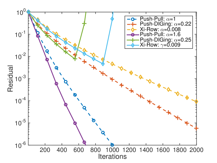
(a) Fixed directed network

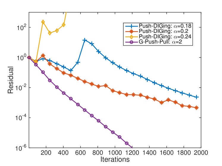
(b) Asynchronous directed network

Figure 2: Plots of (normalized) residuals versus the number of iterations over (a) a fixed directed network and (b) an asynchronous directed network. The simulation results for asynchronous stetting are averaged over 20 runs.

VII Conclusions

In this paper, we have studied the problem of distributed optimization over a network. In particular, we proposed new distributed gradient-based methods (Push-Pull and G-Push-Pull) where each node maintains estimates of the optimal decision variable and the average gradient of the agents’ objective functions. From the viewpoint of an agent, the information about the gradients is pushed to its neighbors, while the information about the decision variable is pulled from its neighbors. The methods utilize two different graphs for the information exchange among agents and work for different types of distributed architecture, including decentralized, centralized, and semi-centralized architecture. We have showed that the algorithms converge linearly for strongly convex and smooth objective functions over a directed network both for synchronous and asynchronous random-gossip updates. In the simulations, we have also demonstrated the effectiveness of the proposed algorithm as compared to the state-of-the-arts.

Appendix A Proofs for Push-Pull

A-A Proof of Lemma 1

Denote by $u_{i}$ the $i$th element of $u$. We first prove that $u_{i}>0$ iff $i\in\mathcal{R}_{\mathbf{R}}$. Note that there exists an order of vertices such that $\mathbf{R}$ can be rewritten as $\tilde{\mathbf{R}}:=\begin{bmatrix}\mathbf{R}_{1}&\mathbf{0}\\ \mathbf{R}_{2}&\mathbf{R}_{3}\end{bmatrix},$ where $\mathbf{R}_{1}$ is a square matrix corresponding to vertices in $\mathcal{R}_{\mathbf{R}}$. Since the induced subgraph $\mathcal{G}_{\mathbf{R}_{1}}$ is strongly connected, $\mathbf{R}_{1}$ is row stochastic and irreducible. In light of the Perron-Frobenius theorem, $\mathbf{R}_{1}$ has a strictly positive left eigenvector $u_{1}^{\intercal}$ (with $u_{1}^{\intercal}\mathbf{1}=n$) corresponding to eigenvalue $1$. It follows that $[u_{1},\mathbf{0}]^{\intercal}$ is a row eigenvector of $\tilde{\mathbf{R}}$, which is also unique from the Perron-Frobenius theorem. Since reordering of vertices does not change the corresponding eigenvector (up to permutation in the same oder of vertices), we have $u_{i}>0$ iff $i\in\mathcal{R}_{\mathbf{R}}$. Similarly, we can show that $v_{j}>0$ iff $j\in\mathcal{R}_{\mathbf{C}^{\intercal}}$. Since $\mathcal{R}_{\mathbf{R}}\cap\mathcal{R}_{\mathbf{C}^{\intercal}}\neq\emptyset$ from Assumption 3, we have $u^{\intercal}v>0$.

A-B Proof of Lemma 2

In light of Assumption 1 and (3), $\|\bar{y}_{k}-g_{k}\|_{2}=\frac{1}{n}\|\mathbf{1}^{\intercal}\nabla F(\mathbf{x}_{k})-\mathbf{1}^{\intercal}\nabla F(\mathbf{1}\bar{x}_{k})\|_{2}\leq\frac{L}{n}\sum_{i=1}^{n}\|x_{i,k}-\bar{x}_{k}\|_{2}\leq\frac{L}{\sqrt{n}}\|\mathbf{x}_{k}-\mathbf{1}\bar{x}_{k}\|_{2},$ and $\|g_{k}\|_{2}=\frac{1}{n}\|\mathbf{1}^{\intercal}\nabla F(\mathbf{1}\bar{x}_{k})-\mathbf{1}^{\intercal}\nabla F(\mathbf{1}x^{*})\|_{2}\leq\frac{L}{n}\sum_{i=1}^{n}\|\bar{x}_{k}-x^{*}\|_{2}=L\|\bar{x}_{k}-x^{*}\|_{2}.$ Proof of the last relation can be found in [5, Lemma 10].

A-C Proof of Lemma 3

In light of [41, Lemma 3.4], under Assumptions 2-3, spectral radii of $\mathbf{R}$ and $\mathbf{C}$ are both equal to $1$ (the corresponding eigenvalues have multiplicity $1$). Suppose for some $\lambda,\tilde{u}\neq 0$, $\tilde{u}^{\intercal}\left(\mathbf{R}-\frac{\mathbf{1}u^{\intercal}}{n}\right)=\lambda\tilde{u}^{\intercal}.$ Since $\mathbf{1}$ is a right eigenvector of $(\mathbf{R}-\mathbf{1}u^{\intercal}/n)$ corresponding to eigenvalue $0$, $\tilde{u}^{\intercal}\mathbf{1}=0$ (see [39, Theorem 1.4.7]). We have $\tilde{u}^{\intercal}\mathbf{R}=\lambda\tilde{u}.$ Hence $\lambda$ is also an eigenvalue of $\mathbf{R}$. Noticing that $u^{\intercal}\mathbf{1}=n$, we have $\tilde{u}^{\intercal}\neq u^{\intercal}$ so that $\lambda<1$. We conclude that $\sigma_{\mathrm{R}}<1$. Similarly we can obtain $\sigma_{\mathrm{C}}<1$.

A-D Proof of Lemma 5

By Definition 1,

$$\begin{array}[]{l}\quad\|W\mathbf{x}\|=\|[\|W\mathbf{x}^{1}\|,\|W\mathbf{x}^{2}\|,\ldots,\|W\mathbf{x}^{p}\|]\|_{2}\\ \leq\|[\|W\|\|\mathbf{x}^{1}\|,\|W\|\|\mathbf{x}^{2}\|,\ldots,\|W\|\|\mathbf{x}^{p}\|]\|_{2}\\ =\|W\|\|[\|\mathbf{x}^{1}\|,\|\mathbf{x}^{2}\|,\ldots,\|\mathbf{x}^{p}\|]\|_{2}=\|W\|\|\mathbf{x}\|,\end{array}$$

and $\|wx\|=\|[\|wx^{1}\|,\|wx^{2}\|,\ldots,\|wx^{p}\|]\|_{2}=\|w\|\|[|x^{1}|,|x^{2}|,\ldots,|x^{p}|]\|_{2}=\|w\|\|x\|_{2}.$

A-E Proof of Lemma 7

The three inequalities embedded in (14) come from (III-A), (12), and (13), respectively. First, by Lemma 2 and Lemma 6, we obtain from (III-A) that

$$\begin{array}[]{l}\quad\|\bar{x}_{k+1}-x^{*}\|_{2}\leq\|\bar{x}_{k}-\alpha^{\prime}g_{k}-x^{*}\|_{2}+\alpha^{\prime}\|\bar{y}_{k}-g_{k}\|_{2}\\ \quad+\frac{1}{n}\|u^{\intercal}\boldsymbol{\alpha}(\mathbf{y}_{k}-v\bar{y}_{k})\|_{2}\\ \leq(1-\alpha^{\prime}\mu)\|\bar{x}_{k}-x^{*}\|_{2}+\frac{\alpha^{\prime}L}{\sqrt{n}}\|\mathbf{x}_{k}-\mathbf{1}\bar{x}_{k}\|_{2}\\ \quad+\frac{\|u\|_{2}\|\boldsymbol{\alpha}\|_{2}}{n}\|\mathbf{y}_{k}-v\bar{y}_{k}\|_{2}\\ \leq(1-\alpha^{\prime}\mu)\|\bar{x}_{k}-x^{*}\|_{2}+\frac{\alpha^{\prime}L}{\sqrt{n}}\|\mathbf{x}_{k}-\mathbf{1}\bar{x}_{k}\|_{\mathrm{R}}\\ \quad+\frac{\hat{\alpha}\|u\|_{2}}{n}\|\mathbf{y}_{k}-v\bar{y}_{k}\|_{\mathrm{C}}.\end{array}$$

Second, by relation (12), Lemma 5 and Lemma 6, we see that

$$\begin{array}[]{l}\quad\|\mathbf{x}_{k+1}-\mathbf{1}\bar{x}_{k+1}\|_{\mathrm{R}}\leq\sigma_{\mathrm{R}}\|\mathbf{x}_{k}-\mathbf{1}\bar{x}_{k}\|_{\mathrm{R}}+\sigma_{\mathrm{R}}\|\boldsymbol{\alpha}\|_{\mathrm{R}}\|\mathbf{y}_{k}\|_{\mathrm{R}}\\ \leq\sigma_{\mathrm{R}}\|\mathbf{x}_{k}-\mathbf{1}\bar{x}_{k}\|_{\mathrm{R}}+\hat{\alpha}\sigma_{\mathrm{R}}\|\mathbf{y}_{k}-v\bar{y}_{k}\|_{\mathrm{R}}+\hat{\alpha}\sigma_{\mathrm{R}}\|v\|_{\mathrm{R}}\|\bar{y}_{k}\|_{2}\\ \leq\sigma_{\mathrm{R}}\|\mathbf{x}_{k}-\mathbf{1}\bar{x}_{k}\|_{\mathrm{R}}+\hat{\alpha}\sigma_{\mathrm{R}}\|\mathbf{y}_{k}-v\bar{y}_{k}\|_{\mathrm{R}}\\ \quad+\hat{\alpha}\sigma_{\mathrm{R}}\|v\|_{\mathrm{R}}\left(\frac{L}{\sqrt{n}}\|\mathbf{x}_{k}-\mathbf{1}\bar{x}_{k}\|_{2}+L\|\bar{x}_{k}-x^{*}\|_{2}\right)\\ \leq\sigma_{\mathrm{R}}\left(1+\hat{\alpha}\|v\|_{\mathrm{R}}\frac{L}{\sqrt{n}}\right)\|\mathbf{x}_{k}-\mathbf{1}\bar{x}_{k}\|_{\mathrm{R}}+\hat{\alpha}\sigma_{\mathrm{R}}\delta_{\mathrm{R},\mathrm{C}}\|\mathbf{y}_{k}-v\bar{y}_{k}\|_{\mathrm{C}}\\ \quad+\hat{\alpha}\sigma_{\mathrm{R}}\|v\|_{\mathrm{R}}L\|\bar{x}_{k}-x^{*}\|_{2}.\end{array}$$

Lastly, it follows from (13), Lemma 5 and Lemma 6 that

$$\begin{array}[]{l}\quad\|\mathbf{y}_{k+1}-v\bar{y}_{k+1}\|_{\mathrm{C}}\leq\sigma_{\mathrm{C}}\|\mathbf{y}_{k}-v\bar{y}_{k}\|_{\mathrm{C}}\\ \quad+c_{0}\delta_{\mathrm{C},2}L\|\mathbf{x}_{k+1}-\mathbf{x}_{k}\|_{2}\\ =\sigma_{\mathrm{C}}\|\mathbf{y}_{k}-v\bar{y}_{k}\|_{\mathrm{C}}+c_{0}\delta_{\mathrm{C},2}L\|(\mathbf{R}-\mathbf{I})(\mathbf{x}_{k}-\mathbf{1}\bar{x}_{k})-\mathbf{R}\boldsymbol{\alpha}\mathbf{y}_{k}\|_{2}\\ \leq\sigma_{\mathrm{C}}\|\mathbf{y}_{k}-v\bar{y}_{k}\|_{\mathrm{C}}+c_{0}\delta_{\mathrm{C},2}L\left(\|\mathbf{R}-\mathbf{I}\|_{2}\|\mathbf{x}_{k}-\mathbf{1}\bar{x}_{k}\|_{2}\right.\\ \quad\left.+\left\|\mathbf{R}\boldsymbol{\alpha}(\mathbf{y}_{k}-v\bar{y}_{k})+\mathbf{R}\boldsymbol{\alpha}v\bar{y}_{k}\right\|_{2}\right)\\ \leq\sigma_{\mathrm{C}}\|\mathbf{y}_{k}-v\bar{y}_{k}\|_{\mathrm{C}}+c_{0}\delta_{\mathrm{C},2}L(\|\mathbf{R}-\mathbf{I}\|_{2}\|\mathbf{x}_{k}-\mathbf{1}\bar{x}_{k}\|_{2}\\ \quad+\|\mathbf{R}\|_{2}\|\boldsymbol{\alpha}\|_{2}\|\mathbf{y}_{k}-v\bar{y}_{k}\|_{2}+\|\mathbf{R}\|_{2}\|\boldsymbol{\alpha}\|_{2}\|v\|_{2}\|\bar{y}_{k}\|_{2}).\end{array}$$

In light of Lemma 2,

$$\|\bar{y}_{k}\|_{2}\leq\left(\frac{L}{\sqrt{n}}\|\mathbf{x}_{k}-\mathbf{1}\bar{x}_{k}\|_{2}+L\|\bar{x}_{k}-x^{*}\|_{2}\right).$$

Hence

$$\begin{array}[]{l}\quad\|\mathbf{y}_{k+1}-v\bar{y}_{k+1}\|_{\mathrm{C}}\\ \leq\left(\sigma_{\mathrm{C}}+\hat{\alpha}c_{0}\delta_{\mathrm{C},2}\|\mathbf{R}\|_{2}L\right)\|\mathbf{y}_{k}-v\bar{y}_{k}\|_{\mathrm{C}}\\ \quad+c_{0}\delta_{\mathrm{C},2}L\|\mathbf{R}-\mathbf{I}\|_{2}\|\mathbf{x}_{k}-\mathbf{1}\bar{x}_{k}\|_{2}\\ \quad+\hat{\alpha}c_{0}\delta_{\mathrm{C},2}\|\mathbf{R}\|_{2}\|v\|_{2}L\left(\frac{L}{\sqrt{n}}\|\mathbf{x}_{k}-\mathbf{1}\bar{x}_{k}\|_{2}+L\|\bar{x}_{k}-x^{*}\|_{2}\right)\\ \leq\left(\sigma_{\mathrm{C}}+\hat{\alpha}c_{0}\delta_{\mathrm{C},2}\|\mathbf{R}\|_{2}L\right)\|\mathbf{y}_{k}-v\bar{y}_{k}\|_{\mathrm{C}}\\ \quad+c_{0}\delta_{\mathrm{C},2}L\left(\|\mathbf{R}-\mathbf{I}\|_{2}+\hat{\alpha}\|\mathbf{R}\|_{2}\|v\|_{2}\frac{L}{\sqrt{n}}\right)\|\mathbf{x}_{k}-\mathbf{1}\bar{x}_{k}\|_{\mathrm{R}}\\ \quad+\hat{\alpha}c_{0}\delta_{\mathrm{C},2}\|\mathbf{R}\|_{2}\|v\|_{2}L^{2}\|\bar{x}_{k}-x^{*}\|_{2}.\end{array}$$

Appendix B Proofs for G-Push-Pull

B-A Proof of Lemma 14

By (43),

$$\begin{array}[]{l}\quad\bar{x}_{k+1}=\frac{\bar{u}^{\intercal}}{n}\left(\mathbf{R}_{k}\mathbf{x}_{k}-\alpha\mathbf{Q}_{k}\mathbf{y}_{k}\right)\\ =\bar{x}_{k}+\frac{\bar{u}^{\intercal}}{n}\left(\tilde{\mathbf{R}}_{k}\mathbf{x}_{k}-\alpha\mathbf{Q}_{k}\mathbf{y}_{k}\right)\\ =\bar{x}_{k}-\alpha\frac{\bar{u}^{\intercal}}{n}\mathbf{Q}_{k}\mathbf{y}_{k}+\frac{\bar{u}^{\intercal}}{n}\tilde{\mathbf{R}}_{k}\left(\mathbf{x}_{k}-\mathbf{1}\bar{x}_{k}\right).\end{array}$$

It follows that

$$\begin{array}[]{l}\quad\|\bar{x}_{k+1}-x^{*}\|_{2}^{2}\\ =\left\|\bar{x}_{k}-\alpha\frac{\bar{u}^{\intercal}}{n}\mathbf{Q}_{k}\mathbf{y}_{k}+\frac{\bar{u}^{\intercal}}{n}\tilde{\mathbf{R}}_{k}\left(\mathbf{x}_{k}-\mathbf{1}\bar{x}_{k}\right)-x^{*}\right\|_{2}^{2}\\ =\|\bar{x}_{k}-x^{*}\|_{2}^{2}\\ \quad-2\left\langle\bar{x}_{k}-x^{*},\alpha\frac{\bar{u}^{\intercal}}{n}\mathbf{Q}_{k}\mathbf{y}_{k}-\frac{\bar{u}^{\intercal}}{n}\tilde{\mathbf{R}}_{k}\left(\mathbf{x}_{k}-\mathbf{1}\bar{x}_{k}\right)\right\rangle\\ \quad+\left\|\alpha\frac{\bar{u}^{\intercal}}{n}\mathbf{Q}_{k}\mathbf{y}_{k}-\frac{\bar{u}^{\intercal}}{n}\tilde{\mathbf{R}}_{k}\left(\mathbf{x}_{k}-\mathbf{1}\bar{x}_{k}\right)\right\|_{2}^{2}.\end{array}$$

Taking conditional expectation on both sides,

$$\begin{array}[]{l}\mathbb{E}\left[\|\bar{x}_{k+1}-x^{*}\|_{2}^{2}\mid\mathcal{H}_{k}\right]=\|\bar{x}_{k}-x^{*}\|_{2}^{2}\\ -2\alpha\left\langle\bar{x}_{k}-x^{*},\frac{\bar{u}^{\intercal}}{n}\mathbb{E}[\mathbf{Q}_{k}]\mathbf{y}_{k}\right\rangle+\alpha^{2}\mathbb{E}\left[\left\|\frac{\bar{u}^{\intercal}}{n}\mathbf{Q}_{k}\mathbf{y}_{k}\right\|_{2}^{2}\mid\mathcal{H}_{k}\right]\\ +\mathbb{E}\left[\left\|\frac{\bar{u}^{\intercal}}{n}\tilde{\mathbf{R}}_{k}\left(\mathbf{x}_{k}-\mathbf{1}\bar{x}_{k}\right)\right\|_{2}^{2}\mid\mathcal{H}_{k}\right].\end{array}$$

We now bound the last two terms on the right-hand side. First,

$$\begin{array}[]{l}\quad\mathbb{E}\left[\left\|\frac{\bar{u}^{\intercal}}{n}\mathbf{Q}_{k}\mathbf{y}_{k}\right\|_{2}^{2}\mid\mathcal{H}_{k}\right]=\mathbf{y}_{k}^{\intercal}\mathbb{E}\left[\mathbf{Q}_{k}^{\intercal}\frac{\bar{u}}{n}\frac{\bar{u}^{\intercal}}{n}\mathbf{Q}_{k}\right]\mathbf{y}_{k}\\ =\mathbf{y}_{k}^{\intercal}\mathbb{E}\left[\mathbf{Q}_{k}^{\intercal}\frac{\bar{u}\bar{u}^{\intercal}}{n^{2}}\mathbf{Q}_{k}\right]\mathbf{y}_{k}\leq\frac{1}{n^{2}}\left\|\mathbb{E}\left[\mathbf{Q}_{k}^{\intercal}\bar{u}\bar{u}^{\intercal}\mathbf{Q}_{k}\right]\right\|_{2}\|\mathbf{y}_{k}\|_{2}^{2}\\ \leq\frac{2}{n^{2}}\left\|\mathbb{E}\left[\mathbf{Q}_{k}^{\intercal}\bar{u}\bar{u}^{\intercal}\mathbf{Q}_{k}\right]\right\|_{2}\left[2\|\mathbf{y}_{k}-\bar{v}\bar{y}_{k}\|_{2}^{2}+2\|\bar{v}\|_{2}^{2}\|\bar{y}_{k}\|_{2}^{2}\right].\end{array}$$

Second,

$$\begin{array}[]{l}\quad\mathbb{E}\left[\left\|\frac{\bar{u}^{\intercal}}{n}\tilde{\mathbf{R}}_{k}\left(\mathbf{x}_{k}-\mathbf{1}\bar{x}_{k}\right)\right\|_{2}^{2}\mid\mathcal{H}_{k}\right]\\ =\left(\mathbf{x}_{k}-\mathbf{1}\bar{x}_{k}\right)^{\intercal}\mathbb{E}\left[\tilde{\mathbf{R}}_{k}^{\intercal}\frac{\bar{u}\bar{u}^{\intercal}}{n^{2}}\tilde{\mathbf{R}}_{k}\right]\left(\mathbf{x}_{k}-\mathbf{1}\bar{x}_{k}\right)\\ \leq\frac{1}{n^{2}}\left\|\mathbb{E}\left[\tilde{\mathbf{R}}_{k}^{\intercal}\bar{u}\bar{u}^{\intercal}\tilde{\mathbf{R}}_{k}\right]\right\|_{2}\|\mathbf{x}_{k}-\mathbf{1}\bar{x}_{k}\|_{2}^{2}.\end{array}$$

The term with inner product can be rewritten in the following way:

$$\begin{array}[]{l}\quad\left\langle\bar{x}_{k}-x^{*},\frac{\bar{u}^{\intercal}}{n}\mathbb{E}[\mathbf{Q}_{k}]\mathbf{y}_{k}\right\rangle=\left\langle\bar{x}_{k}-x^{*},\frac{\bar{u}^{\intercal}}{n}\mathbb{E}[\mathbf{Q}_{k}]\bar{v}\bar{y}_{k}\right\rangle\\ \quad+\left\langle\bar{x}_{k}-x^{*},\frac{\bar{u}^{\intercal}}{n}\mathbb{E}[\mathbf{Q}_{k}](\mathbf{y}_{k}-\bar{v}\bar{y}_{k})\right\rangle\\ =\eta\left\langle\bar{x}_{k}-x^{*},\bar{y}_{k}\right\rangle+\left\langle\bar{x}_{k}-x^{*},\frac{\bar{u}^{\intercal}}{n}\mathbb{E}[\mathbf{Q}_{k}](\mathbf{y}_{k}-\bar{v}\bar{y}_{k})\right\rangle.\end{array}$$

We now have

$$\begin{array}[]{l}\quad\mathbb{E}\left[\|\bar{x}_{k+1}-x^{*}\|_{2}^{2}\mid\mathcal{H}_{k}\right]\\ \leq\|\bar{x}_{k}-x^{*}\|_{2}^{2}-2\alpha\eta\left\langle\bar{x}_{k}-x^{*},\bar{y}_{k}\right\rangle\\ \quad-2\alpha\left\langle\bar{x}_{k}-x^{*},\frac{\bar{u}^{\intercal}}{n}\mathbb{E}[\mathbf{Q}_{k}](\mathbf{y}_{k}-\bar{v}\bar{y}_{k})\right\rangle\\ \quad+\frac{2\alpha^{2}}{{n^{2}}}\left\|\mathbb{E}\left[\mathbf{Q}_{k}^{\intercal}\bar{u}\bar{u}^{\intercal}\mathbf{Q}_{k}\right]\right\|_{2}\|\mathbf{y}_{k}-\bar{v}\bar{y}_{k}\|_{2}^{2}\\ \quad+\frac{2\alpha^{2}}{n^{2}}\left\|\mathbb{E}\left[\mathbf{Q}_{k}^{\intercal}\bar{u}\bar{u}^{\intercal}\mathbf{Q}_{k}\right]\right\|_{2}\|\bar{v}\|_{2}^{2}\|\bar{y}_{k}\|_{2}^{2}\\ \quad+\frac{1}{n^{2}}\left\|\mathbb{E}\left[\tilde{\mathbf{R}}_{k}^{\intercal}\bar{u}\bar{u}^{\intercal}\tilde{\mathbf{R}}_{k}\right]\right\|_{2}\|\mathbf{x}_{k}-\mathbf{1}\bar{x}_{k}\|_{2}^{2}.\end{array}$$

Notice that

$$\begin{array}[]{l}\quad\|\bar{x}_{k}-x^{*}\|_{2}^{2}-2\alpha\eta\left\langle\bar{x}_{k}-x^{*},\bar{y}_{k}\right\rangle\\ =\|\bar{x}_{k}-x^{*}\|_{2}^{2}-2\alpha\eta\left\langle\bar{x}_{k}-x^{*},g_{k}\right\rangle-2\alpha\eta\left\langle\bar{x}_{k}-x^{*},\bar{y}_{k}-g_{k}\right\rangle\\ \leq(1-2\alpha\eta\mu)\|\bar{x}_{k}-x^{*}\|_{2}^{2}-2\alpha\eta\left\langle\bar{x}_{k}-x^{*},\bar{y}_{k}-g_{k}\right\rangle\\ \leq(1-2\alpha\eta\mu)\|\bar{x}_{k}-x^{*}\|_{2}^{2}+2\alpha\eta\|\bar{x}_{k}-x^{*}\|\|\bar{y}_{k}-g_{k}\|,\end{array}$$

and

$$\|\bar{y}_{k}\|_{2}^{2}=\|\bar{y}_{k}-g_{k}+g_{k}\|_{2}^{2}\leq 2\|\bar{y}_{k}-g_{k}\|_{2}^{2}+2\|g_{k}\|_{2}^{2}.$$

We have

$$\begin{array}[]{l}\mathbb{E}\left[\|\bar{x}_{k+1}-x^{*}\|_{2}^{2}\mid\mathcal{H}_{k}\right]\leq(1-2\alpha\eta\mu)\|\bar{x}_{k}-x^{*}\|_{2}^{2}\\ +2\alpha\eta\|\bar{x}_{k}-x^{*}\|_{2}\|\bar{y}_{k}-g_{k}\|_{2}\\ +\frac{2\alpha}{n}\|\bar{x}_{k}-x^{*}\|_{2}\left\|\bar{u}^{\intercal}\mathbb{E}[\mathbf{Q}_{k}]\right\|_{2}\|\mathbf{y}_{k}-\bar{v}\bar{y}_{k}\|_{2}\\ +\frac{2\alpha^{2}}{{n^{2}}}\left\|\mathbb{E}\left[\mathbf{Q}_{k}^{\intercal}\bar{u}\bar{u}^{\intercal}\mathbf{Q}_{k}\right]\right\|_{2}\|\mathbf{y}_{k}-\bar{v}\bar{y}_{k}\|_{2}^{2}\\ +\frac{4\alpha^{2}}{n^{2}}\left\|\mathbb{E}\left[\mathbf{Q}_{k}^{\intercal}\bar{u}\bar{u}^{\intercal}\mathbf{Q}_{k}\right]\right\|_{2}\|\bar{v}\|_{2}^{2}(\|\bar{y}_{k}-g_{k}\|_{2}^{2}+\|g_{k}\|_{2}^{2})\\ +\frac{1}{n^{2}}\left\|\mathbb{E}\left[\tilde{\mathbf{R}}_{k}^{\intercal}\bar{u}\bar{u}^{\intercal}\tilde{\mathbf{R}}_{k}\right]\right\|_{2}\|\mathbf{x}_{k}-\mathbf{1}\bar{x}_{k}\|_{2}^{2}.\end{array}$$

Note that

$$\begin{array}[]{l}\quad 2\alpha\eta\|\bar{x}_{k}-x^{*}\|_{2}\|\bar{y}_{k}-g_{k}\|_{2}\\ \leq\alpha\eta\left(\frac{\mu}{2}\|\bar{x}_{k}-x^{*}\|_{2}^{2}+\frac{2}{\mu}\|\bar{y}_{k}-g_{k}\|_{2}^{2}\right),\end{array}$$

and

$$\begin{array}[]{l}\quad\frac{2\alpha}{n}\|\bar{x}_{k}-x^{*}\|_{2}\left\|\bar{u}^{\intercal}\mathbb{E}[\mathbf{Q}_{k}]\|_{2}\|\mathbf{y}_{k}-\bar{v}\bar{y}_{k}\right\|_{2}\\ \leq\alpha\eta\left(\frac{\mu}{2}\|\bar{x}_{k}-x^{*}\|_{2}^{2}+\frac{2}{\eta^{2}\mu n^{2}}\left\|\bar{u}^{\intercal}\mathbb{E}[\mathbf{Q}_{k}]\right\|_{2}^{2}\|\mathbf{y}_{k}-\bar{v}\bar{y}_{k}\|_{2}^{2}\right).\end{array}$$

From Lemma 2 we obtain

$$\begin{array}[]{l}\quad\mathbb{E}\left[\|\bar{x}_{k+1}-x^{*}\|_{2}^{2}\mid\mathcal{H}_{k}\right]\leq(1-\alpha\eta\mu)\|\bar{x}_{k}-x^{*}\|_{2}^{2}\\ \quad+\frac{2\alpha\eta}{\mu}\|\bar{y}_{k}-g_{k}\|_{2}^{2}+\frac{2\alpha}{\eta\mu n^{2}}\left\|\bar{u}^{\intercal}\mathbb{E}[\mathbf{Q}_{k}]\right\|_{2}^{2}\|\mathbf{y}_{k}-\bar{v}\bar{y}_{k}\|_{2}^{2}\\ \quad+\frac{2\alpha^{2}}{{n^{2}}}\left\|\mathbb{E}\left[\mathbf{Q}_{k}^{\intercal}\bar{u}\bar{u}^{\intercal}\mathbf{Q}_{k}\right]\right\|_{2}\|\mathbf{y}_{k}-\bar{v}\bar{y}_{k}\|_{2}^{2}\\ \quad+\frac{4\alpha^{2}}{n^{2}}\left\|\mathbb{E}\left[\mathbf{Q}_{k}^{\intercal}\bar{u}\bar{u}^{\intercal}\mathbf{Q}_{k}\right]\right\|_{2}\|\bar{v}\|_{2}^{2}(\|\bar{y}_{k}-g_{k}\|_{2}^{2}+\|g_{k}\|_{2}^{2})\\ \quad+\frac{1}{n^{2}}\left\|\mathbb{E}\left[\tilde{\mathbf{R}}_{k}^{\intercal}\bar{u}\bar{u}^{\intercal}\tilde{\mathbf{R}}_{k}\right]\right\|_{2}\|\mathbf{x}_{k}-\mathbf{1}\bar{x}_{k}\|_{2}^{2}\\ \leq\left[1-\alpha\eta\mu+\frac{4\alpha^{2}}{n^{2}}\left\|\mathbb{E}\left[\mathbf{Q}_{k}^{\intercal}\bar{u}\bar{u}^{\intercal}\mathbf{Q}_{k}\right]\right\|_{2}\|\bar{v}\|_{2}^{2}L^{2}\right]\|\bar{x}_{k}-x^{*}\|_{2}^{2}\\ \quad+\left(\frac{2\alpha\eta L^{2}}{\mu n}+\frac{4\alpha^{2}L^{2}}{n^{3}}\left\|\mathbb{E}\left[\mathbf{Q}_{k}^{\intercal}\bar{u}\bar{u}^{\intercal}\mathbf{Q}_{k}\right]\right\|_{2}\|\bar{v}\|_{2}^{2}\right.\\ \quad\left.+\frac{1}{n^{2}}\left\|\mathbb{E}\left[\tilde{\mathbf{R}}_{k}^{\intercal}\bar{u}\bar{u}^{\intercal}\tilde{\mathbf{R}}_{k}\right]\right\|_{2}\right)\|\mathbf{x}_{k}-\mathbf{1}\bar{x}_{k}\|_{2}^{2}\\ \quad+\left(\frac{2\alpha}{\eta\mu n^{2}}\left\|\bar{u}^{\intercal}\mathbb{E}[\mathbf{Q}_{k}]\right\|_{2}^{2}+\frac{2\alpha^{2}}{{n^{2}}}\left\|\mathbb{E}\left[\mathbf{Q}_{k}^{\intercal}\bar{u}\bar{u}^{\intercal}\mathbf{Q}_{k}\right]\right\|_{2}\right)\|\mathbf{y}_{k}-\bar{v}\bar{y}_{k}\|_{2}^{2}.\end{array}$$

B-B Proof of Lemma 16

The first inequality follows directly from Lemma 14 and Lemma 15.

For the second inequality, note that from (46) we have

$$\begin{array}[]{l}\quad\left\|\mathbf{x}_{k+1}-\mathbf{1}\bar{x}_{k+1}\right\|_{\mathrm{S}}^{2}\\ \leq\left[\left\|\left(\mathbf{I}-\frac{\mathbf{1}\bar{u}^{\intercal}}{n}\right)\mathbf{R}_{k}\mathbf{x}_{k}\right\|_{\mathrm{S}}+\left\|\left(\mathbf{I}-\frac{\mathbf{1}\bar{u}^{\intercal}}{n}\right)\alpha\mathbf{Q}_{k}\mathbf{y}_{k}\right\|_{\mathrm{S}}\right]^{2}\\ =\left\|\left(\mathbf{I}-\frac{\mathbf{1}\bar{u}^{\intercal}}{n}\right)\mathbf{R}_{k}\mathbf{x}_{k}\right\|_{\mathrm{S}}^{2}+\alpha^{2}\left\|\left(\mathbf{I}-\frac{\mathbf{1}\bar{u}^{\intercal}}{n}\right)\mathbf{Q}_{k}\mathbf{y}_{k}\right\|_{\mathrm{S}}^{2}\\ \quad+2\alpha\left\|\left(\mathbf{I}-\frac{\mathbf{1}\bar{u}^{\intercal}}{n}\right)\mathbf{R}_{k}\mathbf{x}_{k}\right\|_{\mathrm{S}}\left\|\left(\mathbf{I}-\frac{\mathbf{1}\bar{u}^{\intercal}}{n}\right)\mathbf{Q}_{k}\mathbf{y}_{k}\right\|_{\mathrm{S}}.\end{array}$$

In light of Lemma 12,

$$\begin{array}[]{l}\quad\mathbb{E}\left[\left\|\mathbf{x}_{k+1}-\mathbf{1}\bar{x}_{k+1}\right\|_{\mathrm{S}}^{2}\mid\mathcal{H}_{k}\right]\\ \leq\left(\sigma_{\bar{\mathrm{R}}}+\frac{1-\sigma_{\bar{\mathrm{R}}}}{2}\right)\left\|\mathbf{x}_{k}-\mathbf{1}\bar{x}_{k}\right\|_{\mathrm{S}}^{2}+\alpha^{2}\left(1+\frac{2\sigma_{\bar{\mathrm{R}}}}{1-\sigma_{\bar{\mathrm{R}}}}\right)\|\bar{\mathbf{V}}_{\mathrm{Q}}\|_{2}\|\mathbf{y}_{k}\|_{\mathrm{S}}^{2}\\ =\frac{(1+\sigma_{\bar{\mathrm{R}}})}{2}\left\|\mathbf{x}_{k}-\mathbf{1}\bar{x}_{k}\right\|_{\mathrm{S}}^{2}+\alpha^{2}\left(\frac{1+\sigma_{\bar{\mathrm{R}}}}{1-\sigma_{\bar{\mathrm{R}}}}\right)\|\bar{\mathbf{V}}_{\mathrm{Q}}\|_{2}\|\mathbf{y}_{k}\|_{\mathrm{S}}^{2}.\end{array}$$

Since

$$\begin{array}[]{l}\quad\|\mathbf{y}_{k}\|_{\mathrm{S}}^{2}=\left\|\mathbf{y}_{k}-\bar{v}\bar{y}_{k}+\bar{v}(\bar{y}_{k}-g_{k})+\bar{v}g_{k}\right\|_{\mathrm{S}}^{2}\\ \leq 3\left[\|\mathbf{y}_{k}-\bar{v}\bar{y}_{k}\|_{\mathrm{S}}^{2}+\|\bar{v}\|_{\mathrm{S}}^{2}\|\bar{y}_{k}-g_{k}\|_{2}^{2}+\|\bar{v}\|_{\mathrm{S}}^{2}\|g_{k}\|_{2}^{2}\right]\\ \leq 3\left[\|\mathbf{y}_{k}-\bar{v}\bar{y}_{k}\|_{\mathrm{S}}^{2}+\frac{L^{2}}{n}\|\bar{v}\|_{\mathrm{S}}^{2}\|\mathbf{x}_{k}-\mathbf{1}\bar{x}_{k}\|_{2}^{2}+L^{2}\|\bar{v}\|_{\mathrm{S}}^{2}\|\bar{x}_{k}-x^{*}\|_{2}^{2}\right].\end{array}$$

We have

$$\begin{array}[]{l}\quad\mathbb{E}\left[\left\|\mathbf{x}_{k+1}-\mathbf{1}\bar{x}_{k+1}\right\|_{\mathrm{S}}^{2}\mid\mathcal{H}_{k}\right]\leq\frac{(1+\sigma_{\bar{\mathrm{R}}})}{2}\left\|\mathbf{x}_{k}-\mathbf{1}\bar{x}_{k}\right\|_{\mathrm{S}}^{2}\\ \quad+3\alpha^{2}\left(\frac{1+\sigma_{\bar{\mathrm{R}}}}{1-\sigma_{\bar{\mathrm{R}}}}\right)\|\bar{\mathbf{V}}_{\mathrm{Q}}\|_{2}\left[\|\mathbf{y}_{k}-\bar{v}\bar{y}_{k}\|_{\mathrm{S}}^{2}+\frac{L^{2}}{n}\|\bar{v}\|_{\mathrm{S}}^{2}\|\mathbf{x}_{k}-\mathbf{1}\bar{x}_{k}\|_{2}^{2}\right.\\ \quad+L^{2}\|\bar{v}\|_{\mathrm{S}}^{2}\|\bar{x}_{k}-x^{*}\|_{2}^{2}\Big{]}\\ \leq\left[\frac{(1+\sigma_{\bar{\mathrm{R}}})}{2}+\frac{3\alpha^{2}L^{2}}{n}\left(\frac{1+\sigma_{\bar{\mathrm{R}}}}{1-\sigma_{\bar{\mathrm{R}}}}\right)\|\bar{\mathbf{V}}_{\mathrm{Q}}\|_{2}\|\bar{v}_{\mathrm{S}}\|^{2}\right]\left\|\mathbf{x}_{k}-\mathbf{1}\bar{x}_{k}\right\|_{\mathrm{S}}^{2}\\ \quad+3\alpha^{2}L^{2}\left(\frac{1+\sigma_{\bar{\mathrm{R}}}}{1-\sigma_{\bar{\mathrm{R}}}}\right)\|\bar{\mathbf{V}}_{\mathrm{Q}}\|_{2}\|\bar{v}\|_{\mathrm{S}}^{2}\|\bar{x}_{k}-x^{*}\|_{2}^{2}\\ \quad+3\alpha^{2}\left(\frac{1+\sigma_{\bar{\mathrm{R}}}}{1-\sigma_{\bar{\mathrm{R}}}}\right)\|\bar{\mathbf{V}}_{\mathrm{Q}}\|_{2}\delta_{\mathrm{S},\mathrm{D}}\|\mathbf{y}_{k}-\bar{v}\bar{y}_{k}\|_{\mathrm{D}}^{2}.\end{array}$$

For the last inequality, from (47) and Lemma 13 we have

$$\begin{array}[]{l}\quad\left\|\mathbf{y}_{k+1}-\frac{\bar{v}\mathbf{1}^{\intercal}}{n}\mathbf{y}_{k+1}\right\|_{\mathrm{D}}^{2}\\ \leq\left(\left\|\left(\mathbf{I}-\frac{\bar{v}\mathbf{1}^{\intercal}}{n}\right)\mathbf{C}_{k}\mathbf{y}_{k}\right\|_{\mathrm{D}}\right.\\ \quad\left.+\left\|\left(\mathbf{I}-\frac{\bar{v}\mathbf{1}^{\intercal}}{n}\right)\left[\nabla F(\mathbf{x}_{k+1})-\nabla F(\mathbf{x}_{k})\right]\right\|_{\mathrm{D}}\right)^{2}\\ \leq\left(1+\frac{1-\sigma_{\bar{\mathrm{C}}}}{2\sigma_{\bar{\mathrm{C}}}}\right)\left(\sigma_{\bar{\mathrm{C}}}\left\|\mathbf{y}_{k}-\bar{v}\bar{y}_{k}\right\|_{\mathrm{D}}^{2}+2\gamma^{2}\|\bar{\mathbf{V}}_{\mathrm{E}}\|_{2}\left\|\bar{v}\bar{y}_{k}\right\|_{\mathrm{D}}^{2}\right)\\ \quad+\left(1+\frac{2\sigma_{\bar{\mathrm{C}}}}{1-\sigma_{\bar{\mathrm{C}}}}\right)\left\|\left(\mathbf{I}-\frac{\bar{v}\mathbf{1}^{\intercal}}{n}\right)\left[\nabla F(\mathbf{x}_{k+1})-\nabla F(\mathbf{x}_{k})\right]\right\|_{\mathrm{D}}^{2}\\ =\frac{(1+\sigma_{\bar{\mathrm{C}}})}{2}\left\|\mathbf{y}_{k}-\bar{v}\bar{y}_{k}\right\|_{\mathrm{D}}^{2}+\frac{(1+\sigma_{\bar{\mathrm{C}}})}{\sigma_{\bar{\mathrm{C}}}}\gamma^{2}\|\bar{\mathbf{V}}_{\mathrm{E}}\|_{2}\left\|\bar{v}\bar{y}_{k}\right\|_{\mathrm{D}}^{2}\\ \quad+\left(\frac{1+\sigma_{\bar{\mathrm{C}}}}{1-\sigma_{\bar{\mathrm{C}}}}\right)\left\|\left(\mathbf{I}-\frac{\bar{v}\mathbf{1}^{\intercal}}{n}\right)\left[\nabla F(\mathbf{x}_{k+1})-\nabla F(\mathbf{x}_{k})\right]\right\|_{\mathrm{D}}^{2}.\end{array}$$

Notice that by (43) and Assumption 1,

$$\begin{array}[]{l}\quad\|\nabla F(\mathbf{x}_{k+1})-\nabla F(\mathbf{x}_{k})\|_{\mathrm{D}}^{2}\leq\delta_{\mathrm{D},2}^{2}L^{2}\|\mathbf{x}_{k+1}-\mathbf{x}_{k}\|_{2}^{2}\\ =\delta_{\mathrm{D},2}^{2}L^{2}\|\mathbf{R}_{k}\mathbf{x}_{k}-\alpha\mathbf{Q}_{k}\mathbf{y}_{k}-\mathbf{x}_{k}\|_{2}^{2}\\ \leq 2\delta_{\mathrm{D},2}^{2}L^{2}\|(\mathbf{R}_{k}-\mathbf{I})(\mathbf{x}_{k}-\mathbf{1}\bar{x}_{k})\|_{2}^{2}+2\alpha^{2}\delta_{\mathrm{D},2}^{2}L^{2}\|\mathbf{Q}_{k}\|_{2}^{2}\|\mathbf{y}_{k}\|_{2}^{2}\\ \leq 2\delta_{\mathrm{D},2}^{2}L^{2}\|\mathbf{R}_{k}-\mathbf{I}\|_{2}^{2}\|\mathbf{x}_{k}-\mathbf{1}\bar{x}_{k}\|_{2}^{2}\\ \quad+4\alpha^{2}\delta_{\mathrm{D},2}^{2}L^{2}\|\mathbf{Q}_{k}\|_{2}^{2}(\|\mathbf{y}_{k}-\bar{v}\bar{y}_{k}\|_{2}^{2}+\|\bar{v}\bar{y}_{k}\|_{2}^{2}).\end{array}$$

We have

$$\begin{array}[]{l}\quad\left\|\mathbf{y}_{k+1}-\bar{v}\bar{y}_{k+1}\right\|_{\mathrm{D}}^{2}\leq\frac{(1+\sigma_{\bar{\mathrm{C}}})}{2}\left\|\mathbf{y}_{k}-\bar{v}\bar{y}_{k}\right\|_{\mathrm{D}}^{2}\\ \quad+\frac{(1+\sigma_{\bar{\mathrm{C}}})}{\sigma_{\bar{\mathrm{C}}}}\gamma^{2}\|\bar{\mathbf{V}}_{\mathrm{E}}\|_{2}\left\|\bar{v}\bar{y}_{k}\right\|_{\mathrm{D}}^{2}\\ \quad+\delta_{\mathrm{D},2}^{2}L^{2}\left(\frac{1+\sigma_{\bar{\mathrm{C}}}}{1-\sigma_{\bar{\mathrm{C}}}}\right)\left\|\mathbf{I}-\frac{\bar{v}\mathbf{1}^{\intercal}}{n}\right\|_{\mathrm{D}}^{2}\left[2\|\mathbf{R}_{k}-\mathbf{I}\|_{2}^{2}\|\mathbf{x}_{k}-\mathbf{1}\bar{x}_{k}\|_{2}^{2}\right.\\ \quad\left.+4\alpha^{2}\|\mathbf{Q}_{k}\|_{2}^{2}(\|\mathbf{y}_{k}-\bar{v}\bar{y}_{k}\|_{2}^{2}+\|\bar{v}\bar{y}_{k}\|_{2}^{2})\right]\\ \leq\left[\frac{(1+\sigma_{\bar{\mathrm{C}}})}{2}+4\alpha^{2}\delta_{\mathrm{D},2}^{2}L^{2}\left(\frac{1+\sigma_{\bar{\mathrm{C}}}}{1-\sigma_{\bar{\mathrm{C}}}}\right)\left\|\mathbf{I}-\frac{\bar{v}\mathbf{1}^{\intercal}}{n}\right\|_{\mathrm{D}}^{2}\|\mathbf{Q}_{k}\|_{2}^{2}\right]\\ \quad\cdot\left\|\mathbf{y}_{k}-\bar{v}\bar{y}_{k}\right\|_{2}^{2}\\ \quad+2\delta_{\mathrm{D},2}^{2}L^{2}\left(\frac{1+\sigma_{\bar{\mathrm{C}}}}{1-\sigma_{\bar{\mathrm{C}}}}\right)\left\|\mathbf{I}-\frac{\bar{v}\mathbf{1}^{\intercal}}{n}\right\|_{\mathrm{D}}^{2}\|\mathbf{R}_{k}-\mathbf{I}\|_{2}^{2}\|\mathbf{x}_{k}-\mathbf{1}\bar{x}_{k}\|_{2}^{2}\\ \quad+\left[\frac{(1+\sigma_{\bar{\mathrm{C}}})}{\sigma_{\bar{\mathrm{C}}}}\gamma^{2}\|\bar{\mathbf{V}}_{\mathrm{E}}\|_{2}\|\bar{v}\|_{\mathrm{D}}^{2}\right.\\ \quad\left.+4\alpha^{2}\delta_{\mathrm{D},2}^{2}L^{2}\left(\frac{1+\sigma_{\bar{\mathrm{C}}}}{1-\sigma_{\bar{\mathrm{C}}}}\right)\left\|\mathbf{I}-\frac{\bar{v}\mathbf{1}^{\intercal}}{n}\right\|_{\mathrm{D}}^{2}\|\mathbf{Q}_{k}\|_{2}^{2}\|\bar{v}\|_{2}^{2}\right]\left\|\bar{y}_{k}\right\|_{2}^{2}\\ \leq\left[\frac{(1+\sigma_{\bar{\mathrm{C}}})}{2}+4\alpha^{2}\delta_{\mathrm{D},2}^{2}L^{2}\left(\frac{1+\sigma_{\bar{\mathrm{C}}}}{1-\sigma_{\bar{\mathrm{C}}}}\right)\left\|\mathbf{I}-\frac{\bar{v}\mathbf{1}^{\intercal}}{n}\right\|_{\mathrm{D}}^{2}\|\mathbf{Q}_{k}\|_{2}^{2}\right]\\ \quad\cdot\left\|\mathbf{y}_{k}-\bar{v}\bar{y}_{k}\right\|_{\mathrm{D}}^{2}\\ \quad+2\delta_{\mathrm{D},2}^{2}L^{2}\left(\frac{1+\sigma_{\bar{\mathrm{C}}}}{1-\sigma_{\bar{\mathrm{C}}}}\right)\left\|\mathbf{I}-\frac{\bar{v}\mathbf{1}^{\intercal}}{n}\right\|_{\mathrm{D}}^{2}\|\mathbf{R}_{k}-\mathbf{I}\|_{2}^{2}\|\mathbf{x}_{k}-\mathbf{1}\bar{x}_{k}\|_{\mathrm{S}}^{2}\\ \quad+2L^{2}\left[\frac{(1+\sigma_{\bar{\mathrm{C}}})}{\sigma_{\bar{\mathrm{C}}}}\gamma^{2}\|\bar{\mathbf{V}}_{\mathrm{E}}\|_{2}\|\bar{v}\|_{\mathrm{D}}^{2}\right.\\ \quad\left.+4\alpha^{2}\delta_{\mathrm{D},2}^{2}L^{2}\left(\frac{1+\sigma_{\bar{\mathrm{C}}}}{1-\sigma_{\bar{\mathrm{C}}}}\right)\left\|\mathbf{I}-\frac{\bar{v}\mathbf{1}^{\intercal}}{n}\right\|_{\mathrm{D}}^{2}\|\mathbf{Q}_{k}\|_{2}^{2}\|\bar{v}\|_{2}^{2}\right]\\ \quad\cdot\left(\frac{1}{n}\|\mathbf{x}_{k}-\mathbf{1}\bar{x}_{k}\|_{2}^{2}+\|\bar{x}_{k}-x^{*}\|_{2}^{2}\right).\end{array}$$

Shi Pu is currently an assistant professor in the Institute for Data and Decision Analytics, The Chinese University of Hong Kong, Shenzhen, China. He received a B.S. Degree in Engineering Mechanics from Peking University, in 2012, and a Ph.D. Degree in Systems Engineering from the University of Virginia, in 2016. He was a postdoctoral associate at the University of Florida, from 2016 to 2017, a postdoctoral scholar at Arizona State University, from 2017 to 2018, and a postdoctoral associate at Boston University, from 2018 to 2019. His research interests include distributed optimization, network science, machine learning, and game theory.

Wei (Wilbur) Shi was a postdoc in the Electrical and Computer Engineering Department of Princeton University, Princeton, NJ, USA. He obtained his Ph.D. in Control Science and Engineering from the University of Science and Technology of China, Hefei, Anhui, China. He was a postdoc in the Coordinated Science Laboratory, University of Illinois at Urbana-Champaign, Urbana, IL, USA. His current research interest distributes in optimization, learning, and control, and applications in cyber physical systems and internet of things. He was a recipient of the Young Author Best Paper Award in IEEE Signal Processing Society.

Jinming Xu received the B.S. degree in mechanical engineering from Shandong University, China, in 2009 and the Ph.D. degree in Electrical and Electronic Engineering from Nanyang Technological University (NTU), Singapore, in 2016. He was a research fellow of the EXQUITUS center at NTU from 2016 to 2017; he also received postdoctoral training in the Ira A. Fulton Schools of Engineering, Arizona State University, from 2017 to 2018, and School of Industrial Engineering, Purdue University, from 2018 to 2019, respectively. Currently, he is an assistant professor with the College of Control Science and Engineering at Zhejiang University, China. His research interests include distributed optimization and control, machine learning and network science.

Angelia Nedić has a Ph.D. from Moscow State University, Moscow, Russia, in Computational Mathematics and Mathematical Physics (1994), and a Ph.D. from Massachusetts Institute of Technology, Cambridge, USA in Electrical and Computer Science Engineering (2002). She has worked as a senior engineer in BAE Systems North America, Advanced Information Technology Division at Burlington, MA. Currently, she is a faculty member of the school of Electrical, Computer and Energy Engineering at Arizona State University at Tempe. Prior to joining Arizona State University, she has been a Willard Scholar faculty member at the University of Illinois at Urbana-Champaign. She is a recipient (jointly with her co-authors) of the Best Paper Awards at the Winter Simulation Conference 2013 and at the International Symposium on Modeling and Optimization in Mobile, Ad Hoc and Wireless Networks (WiOpt) 2015. Her general research interest is in optimization, large scale complex systems dynamics, variational inequalities and games.

References

- [1] S. Pu, W. Shi, J. Xu, and A. Nedić, “A push-pull gradient method for distributed optimization in networks,” in Proceedings of the 54th IEEE Conference on Decision and Control (CDC), 2018.
- [2] W. Shi, Q. Ling, K. Yuan, G. Wu, and W. Yin, “On the Linear Convergence of the ADMM in Decentralized Consensus Optimization,” IEEE Transactions on Signal Processing, vol. 62, no. 7, pp. 1750–1761, 2014.
- [3] W. Shi, Q. Ling, G. Wu, and W. Yin, “EXTRA: An Exact First-Order Algorithm for Decentralized Consensus Optimization,” SIAM Journal on Optimization, vol. 25, no. 2, pp. 944–966, 2015.
- [4] A. Olshevsky, “Linear time average consensus and distributed optimization on fixed graphs,” SIAM Journal on Control and Optimization, vol. 55, no. 6, pp. 3990–4014, 2017.
- [5] G. Qu and N. Li, “Harnessing smoothness to accelerate distributed optimization,” IEEE Transactions on Control of Network Systems, 2017.
- [6] K. Scaman, F. Bach, S. Bubeck, Y. T. Lee, and L. Massoulié, “Optimal algorithms for smooth and strongly convex distributed optimization in networks,” in International Conference on Machine Learning, 2017, pp. 3027–3036.
- [7] A. Nedic and A. Ozdaglar, “Distributed subgradient methods for multi-agent optimization,” IEEE Transactions on Automatic Control, vol. 54, no. 1, pp. 48–61, 2009.
- [8] J. Xu, S. Zhu, Y. C. Soh, and L. Xie, “Convergence of asynchronous distributed gradient methods over stochastic networks,” IEEE Transactions on Automatic Control, 2017.
- [9] A. Nedić, A. Olshevsky, and W. Shi, “Achieving geometric convergence for distributed optimization over time-varying graphs,” SIAM Journal on Optimization, vol. 27, no. 4, pp. 2597–2633, 2017.
- [10] A. Nedić and A. Olshevsky, “Distributed optimization over time-varying directed graphs,” IEEE Transactions on Automatic Control, vol. 60, no. 3, pp. 601–615, 2015.
- [11] ——, “Stochastic gradient-push for strongly convex functions on time-varying directed graphs,” IEEE Transactions on Automatic Control, vol. 61, no. 12, pp. 3936–3947, 2016.
- [12] J. Zeng and W. Yin, “Extrapush for convex smooth decentralized optimization over directed networks,” Journal of Computational Mathematics, vol. 35, no. 4, 2017.
- [13] C. Xi and U. A. Khan, “Dextra: A fast algorithm for optimization over directed graphs,” IEEE Transactions on Automatic Control, vol. 62, no. 10, pp. 4980–4993, 2017.
- [14] C. Xi, V. S. Mai, R. Xin, E. H. Abed, and U. A. Khan, “Linear convergence in optimization over directed graphs with row-stochastic matrices,” IEEE Transactions on Automatic Control, 2018.
- [15] S. Boyd, N. Parikh, E. Chu, B. Peleato, J. Eckstein et al., “Distributed optimization and statistical learning via the alternating direction method of multipliers,” Foundations and Trends® in Machine Learning, vol. 3, no. 1, pp. 1–122, 2011.
- [16] Z. Peng, Y. Xu, M. Yan, and W. Yin, “Arock: an algorithmic framework for asynchronous parallel coordinate updates,” SIAM Journal on Scientific Computing, vol. 38, no. 5, pp. A2851–A2879, 2016.
- [17] A. Nedić, A. Olshevsky, and M. G. Rabbat, “Network topology and communication-computation tradeoffs in decentralized optimization,” Proceedings of the IEEE, vol. 106, no. 5, pp. 953–976, 2018.
- [18] S. Boyd, A. Ghosh, B. Prabhakar, and D. Shah, “Randomized gossip algorithms,” IEEE transactions on information theory, vol. 52, no. 6, pp. 2508–2530, 2006.
- [19] J. Lu, C. Y. Tang, P. R. Regier, and T. D. Bow, “Gossip algorithms for convex consensus optimization over networks,” IEEE Transactions on Automatic Control, vol. 56, no. 12, pp. 2917–2923, 2011.
- [20] S. Lee and A. Nedić, “Asynchronous gossip-based random projection algorithms over networks,” IEEE Transactions on Automatic Control, vol. 61, no. 4, pp. 953–968, 2016.
- [21] A. S. Mathkar and V. S. Borkar, “Nonlinear gossip,” SIAM Journal on Control and Optimization, vol. 54, no. 3, pp. 1535–1557, 2016.
- [22] A. Mokhtari, W. Shi, Q. Ling, and A. Ribeiro, “A decentralized second-order method with exact linear convergence rate for consensus optimization,” IEEE Transactions on Signal and Information Processing over Networks, vol. 2, no. 4, pp. 507–522, 2016.
- [23] D. Varagnolo, F. Zanella, A. Cenedese, G. Pillonetto, and L. Schenato, “Newton-raphson consensus for distributed convex optimization,” IEEE Transactions on Automatic Control, vol. 61, no. 4, pp. 994–1009, 2016.
- [24] C. A. Uribe, S. Lee, A. Gasnikov, and A. Nedić, “Optimal algorithms for distributed optimization,” arXiv preprint arXiv:1712.00232, 2017.
- [25] J. Xu, S. Zhu, Y. C. Soh, and L. Xie, “Augmented distributed gradient methods for multi-agent optimization under uncoordinated constant stepsizes,” in Decision and Control (CDC), 2015 IEEE 54th Annual Conference on. IEEE, 2015, pp. 2055–2060.
- [26] A. Nedić, A. Olshevsky, W. Shi, and C. A. Uribe, “Geometrically convergent distributed optimization with uncoordinated step-sizes,” in American Control Conference (ACC), 2017. IEEE, 2017, pp. 3950–3955.
- [27] P. Di Lorenzo and G. Scutari, “Next: In-network nonconvex optimization,” IEEE Transactions on Signal and Information Processing over Networks, vol. 2, no. 2, pp. 120–136, 2016.
- [28] W. Shi, Q. Ling, G. Wu, and W. Yin, “A Proximal Gradient Algorithm for Decentralized Composite Optimization,” IEEE Transactions on Signal Processing, vol. 63, no. 22, pp. 6013–6023, 2015.
- [29] Z. Li, W. Shi, and M. Yan, “A decentralized proximal-gradient method with network independent step-sizes and separated convergence rates,” IEEE Transactions on Signal Processing, vol. 67, no. 17, pp. 4494–4506, 2019.
- [30] T. Wu, K. Yuan, Q. Ling, W. Yin, and A. H. Sayed, “Decentralized consensus optimization with asynchrony and delays,” in Signals, Systems and Computers, 2016 50th Asilomar Conference on. IEEE, 2016, pp. 992–996.
- [31] S. Pu and A. Garcia, “Swarming for faster convergence in stochastic optimization,” SIAM Journal on Control and Optimization, vol. 56, no. 4, pp. 2997–3020, 2018.
- [32] S. Pu and A. Nedić, “Distributed stochastic gradient tracking methods,” arXiv preprint arXiv:1805.11454, 2018.
- [33] D. Kempe, A. Dobra, and J. Gehrke, “Gossip-Based Computation of Aggregate Information,” in Proceedings of the 44th Annual IEEE Symposium on Foundations of Computer Science, 2003, pp. 482–491.
- [34] K. I. Tsianos, S. Lawlor, and M. G. Rabbat, “Push-sum distributed dual averaging for convex optimization,” in Decision and Control (CDC), 2012 IEEE 51st Annual Conference on. IEEE, 2012, pp. 5453–5458.
- [35] R. Xin, C. Xi, and U. A. Khan, “Frost—fast row-stochastic optimization with uncoordinated step-sizes,” EURASIP Journal on Advances in Signal Processing, vol. 2019, no. 1, pp. 1–14, 2019.
- [36] R. Xin and U. A. Khan, “A linear algorithm for optimization over directed graphs with geometric convergence,” IEEE Control Systems Letters, vol. 2, no. 3, pp. 315–320, 2018.
- [37] C. Godsil and G. F. Royle, Algebraic graph theory. Springer Science & Business Media, 2013, vol. 207.
- [38] K. Cai and H. Ishii, “Average consensus on general strongly connected digraphs,” Automatica, vol. 48, no. 11, pp. 2750–2761, 2012.
- [39] R. A. Horn and C. R. Johnson, Matrix analysis. Cambridge university press, 1990.
- [40] A. Sayed, “Diffusion Adaptation over Networks,” Academic Press Library in Signal Processing, vol. 3, pp. 323–454, 2013.
- [41] W. Ren and R. W. Beard, “Consensus seeking in multiagent systems under dynamically changing interaction topologies,” IEEE Transactions on automatic control, vol. 50, no. 5, pp. 655–661, 2005.