Gravitoturbulent dynamos in astrophysical discs

Abstract

The origin of large-scale and coherent magnetic fields in astrophysical discs is an important and long standing problem. Researchers commonly appeal to a turbulent dynamo, sustained by the magneto-rotational instability (MRI), to supply the large-scale field. But research over the last decade in particular has demonstrated that various non-ideal MHD effects can impede or extinguish the MRI, especially in protoplanetary disks. In this paper we propose a new scenario, by which the magnetic field is generated and sustained via the gravitational instability (GI). We use 3D stratified shearing box simulations to characterise the dynamo and find that it works at low magnetic Reynolds number (from unity to $\sim 100$) for a wide range of cooling times and boundary conditions. The process is kinematic, with a relatively fast growth rate ($\lesssim 0.1\Omega$), and it shares some properties of mean field dynamos. The magnetic field is generated via the combination of differential rotation and spiral density waves, the latter providing compressible horizontal motions and large-scale vertical rolls. At greater magnetic Reynolds numbers the build up of large-scale field is diminished and instead small-scale structures emerge from the breakdown of twisted flux ropes. We propose that GI may be key to the dynamo engine not only in young protoplanetary discs but also in some AGN and galaxies.

1 Introduction

Magnetic fields appear in almost all astrophysical discs, from those surrounding newly born stars, active galactic nuclei (AGN), dwarf novae and low-mass X-ray binaries, to spiral galaxies. They are thought to guide the evolution of these objects via several processes, such as accretion, outbursts, winds, and turbulence (Balbus, 2003; Wardle, 2007; Armitage, 2015). In several protoplanetary (PP) discs, indirect observations, based on polarized synchrotron or dust emission, have detected magnetic fields with various strengths and morphologies (Carrasco-González et al., 2010; Stephens et al., 2014; Goddi et al., 2017). In fact, in the bulk of the FU-Ori disc, fields have been observed directly, using the high-resolution spectropolarimeter ESPaDOnS (Donati et al., 2005). On the other hand, magnetic fields appear in many galactic discs, with a horizontal bisymmetric-spiral component (e.g. M51, Fletcher et al., 2011) and in our own galaxy, with a vertical structure recently determined by the Planck satellite using the cosmic background polarization. Fields in AGN and mass-transferring binaries have not been detected directly, but their existence can be inferred from the magnetised jets launched from their associated disks.

A fundamental goal is to determine the origin of these magnetic fields and their sustenance over the disc’s life. In the case of PP discs (the main focus of our paper), it is possible that the fields issue from the central protostar or are inherited from the primordial nebulae. If the latter, then the transport and amplification of magnetic field through the disk are key, and these processes remain the focus of current research (Guilet & Ogilvie, 2013; Zhu & Stone, 2018). Another possibility is that the field is produced in-situ by a turbulent dynamo. This idea, originally suggested by Pudritz (1981), was bolstered by the observations of Donati et al. (2005) which revealed a complex magnetic topology, with both filamentary and toroidal structures, possibly generated by motions internal to the disc. Such an in-situ process is appealing because of its generality: PP disks need not rely on the particularities of any external magnetic source; it might also generalise to AGN and galactic disks.

For more than two decades, the magnetorotational instability (MRI) has been proposed as a potential source of turbulence and magnetic fields in these objects (Balbus & Hawley, 1991; Hawley et al., 1995; Brandenburg et al., 1995; Balbus & Henri, 2008), via a subcritical, nonlinear, and cyclic dynamo. That said, in PP discs, this process has been shown to work reliably only in their very inner radii ($\lesssim 0.1-1$ AU), where ionization sources are strong enough to permit the MRI. Further out, non-ideal MHD effects (Ohmic and ambipolar diffusion plus the Hall effect) tend to weaken or quench the MRI (Wardle, 1999; Sano et al., 2000; Fleming et al., 2000; Kunz & Balbus, 2004; Wardle & Salmeron, 2012; Bai, 2013; Lesur et al., 2014; Bai, 2015). So too in AGN; close to the supermassive black hole the disc is well coupled to the magnetic field, but outward of 0.01 pc the state of the gas is far less clear, as it depends on uncertain non-thermal ionisation sources and the degree of disk warping (e.g. Menou & Quataert, 2001). Putting ionisation aside, several numerical studies have suggested that the MRI dynamo is suppressed in many of these settings because of their low magnetic Prandtl number (ratio between the microscopic viscosity and resistivity; see Fromang et al., 2007; Balbus & Henri, 2008; Käpylä & Korpi, 2011; Meheut et al., 2015; Riols et al., 2017b, for more details).

An alternative to the MRI is growth of magnetic fields via other disc instabilities. Perhaps the most efficient and powerful, after the MRI, is the gravitational instability (GI; for the PP disk context see reviews by Durisen et al., 2007; Kratter & Lodato, 2016). Discs are usually susceptible to the GI in their outer regions, provided that

$$Q=\dfrac{c_{s}\Omega}{\pi G\Sigma_{0}}\lesssim 1$$ (1)

where $Q$ is the Toomre parameter (Toomre, 1964), $c_{s}$ is the sound speed, $\Omega$ the orbital frequency, and $\Sigma_{0}$ the background surface density. It is believed that 50% of class 0 and 10-20% of class I PP discs might be unstable to GI (Tobin et al., 2013; Mann et al., 2015). In particular, the detection of spiral arms and streamers, recently imaged at NIR wavelengths in Ophiuchi and FU Ori systems, supports the idea that their discs are gravitationally unstable (Christiaens et al., 2014; Liu et al., 2016; Dong et al., 2016). Because they are thin, AGN are also susceptible to GI in the regions beyond 0.01 pc and might build up magnetic fields through this process (Menou & Quataert, 2001; Goodman, 2003; Lodato, 2007). The instability, of course, features also in galactic discs (perhaps its most famous venue), shaping the large-scale spiral and clumpy structures where stars form (Goldreich & Lynden-Bell, 1965; Wang & Silk, 1994; Kim & Ostriker, 2001).

The ability of GI to amplify seed magnetic fields has been pointed out in the context of star formation (i.e during the collapse of self-gravitating dense cloud, see Pudritz & Silk, 1989; Federrath et al., 2011). However, the viability of a GI-reliant dynamo process is relatively unexplored in the accretion disc context. The recent shearing box simulations of Riols & Latter (2018a, hereafter RL18a) showed that such a dynamo does exist and can sustain magnetic fields to near equipartition values, especially in the regime of efficient cooling; in addition, GI impedes the (zero-net flux) MRI in this regime. However, most of the simulations were run in the “ideal limit" (i.e. without explicit diffusion), omitting all the relevant non-ideal effects, such as resistivity, the Hall effect, and ambipolar diffusion, each potentially important in the regions of PP discs where GI is active (see Simon et al., 2015, for instance). Moreover, no theory was proposed that could account for the properties of, and physical mechanism animating, the GI dynamo. This paper is a first in a series that aims to address these issues and lay the foundations of a general theory. Here, we only focus on ohmic resistivity, so as to more easily characterize the dynamo’s fundamental nature: is it kinematic or nonlinear? Fast or slow? Small or large scale?. We stress that the present study is a preliminary and necessary step before including other non-ideal physics. However, we point out that both ambipolar diffusion and the Hall effect are necessarily absent in the kinematic phase of any dynamo, and so during this initial phase our results are broadly applicable.

To that end, we perform 3D MHD stratified shearing box simulations with self-gravity using a modified version of the PLUTO code. Simulations maintain a quasi-steady energy balance via inclusion of a simple linear cooling law, characterised by a uniform and constant timescale $\tau_{c}$, and enforce a zero-net vertical magnetic flux. We explore a range of magnetic Reynolds numbers, from 1 to about 500, defined with respect to the sound speed and disc scaleheight. It is important to note that the MRI is excluded in this regime (Simon et al., 2012), and so any magnetic field generation must issue from GI-turbulent motions. Given the size of the box necessary to capture GI, it is not yet possible to probe the regime of Rm larger than a thousand, typically found in the inner ($\lesssim$0.1 AU) and external regions ($\gtrsim$ 20 AU) of older PP disc, and in other environments like AGN.

We find that the GI-dynamo is inherently kinematic and linear, with growth rates depending strongly on Rm. The dynamo process persists even in a very resistive plasma with typical $\text{Rm}\simeq 1$, and appears to be robust even when GI is weak. At lowish Rm ($\lesssim 100$), a very efficient dynamo, supported by the combined action of shear (the “omega effect”) and spiral wave motions, amplifies and organises the magnetic field into large-scale spiral patterns. Essential ingredients in the dynamo are the vertical rolls associated with spirals waves (Riols & Latter, 2018b, hereafter RL18b) which allow the regeneration of the mean poloidal field from toroidal field, through a very unusual “alpha" effect. At larger Rm ($\gtrsim 100$), the dynamo persists but saturates at a lower amplitude. In this regime the large-scale field ropes are twisted and break down into small-scale filamentary structures with a concomitant alteration of the mean-field dynamo effect.

The structure of the paper is as follows: first, in Section 2, we present the basic equations of the problem and the numerical methods. In Section 3 we study the dynamo growth rate and saturated state as a function of Rm. In Section 4, we characterise the essence of the dynamo process and its typical scales. In Section 5 we investigate in more detail the role of spiral waves in the generation of large-scale and also small-scale fields. We discuss in Section 6 the dependence of the dynamo on numerical details (boundary conditions, numerical resolution) and its applications to protoplanetary discs and galaxies. Finally, we state our conclusions in Section 7.

2 Numerical model

2.1 Governing equations

We use the local Cartesian model of an accretion disc (the shearing sheet; Goldreich & Lynden-Bell, 1965; Latter & Papaloizou, 2017) where the differential rotation is approximated locally by a linear shear flow $-S\mathbf{e}_{y}$ and a uniform rotation rate $\bm{\Omega}=\Omega\,\mathbf{e}_{z}$, with $S=(3/2)\,\Omega$ for a Keplerian equilibrium. We denote $(x,y,z)$ as the radial, azimuthal and vertical directions respectively, and refer to the $(x,z)$ projections of vector fields as their poloidal components and to the $y$ component as their toroidal one. We assume that the gas orbiting around the central object is ideal, its pressure $P$ and density $\rho$ related by $\gamma P=\rho c_{s}^{2}$, where $c_{s}$ is the sound speed and $\gamma=5/3$ the ratio of specific heats. In this paper, we neglect molecular viscosity but will consider non-zero uniform magnetic diffusivity $\eta$.A uniform $\eta$ greatly simplifies the problem, although it is not especially realistic. In PP discs, outside of 1 AU, the ionisation fraction (and consequently $\eta$) depends strongly on $z$, due to irradiation by cosmic, FUV, and X rays. We assume for the moment that this variation does not significantly influence the dynamo process. Future simulations will explore a height dependent $\eta$, using realistic profiles such as in Simon et al. (2015).

The evolution of density ${\rho}$, total velocity field $\mathbf{v}$, magnetic field $\mathbf{B}$ and total energy density $e_{t}=\dfrac{1}{2}\rho\mathbf{v}^{2}+\mathbf{B}^{2}/2+P/(\gamma-1)$ follows:

$$\dfrac{\partial\rho}{\partial t}+\nabla\cdot\left(\rho\mathbf{v}\right)=0$$ (2)

$$\frac{\partial{\mathbf{v}}}{\partial{t}}+\mathbf{v}\cdot\mathbf{\nabla v}+2\bm{\Omega}\times\mathbf{v}=-\nabla\Phi-\dfrac{\mathbf{\nabla}{P}}{\rho}+\dfrac{(\nabla\times\mathbf{B})\times\mathbf{B}}{\rho},$$ (3)

$$\frac{\partial{\mathbf{B}}}{\partial{t}}=-\nabla\times\mathbf{E},$$ (4)

$${\dfrac{\partial e_{t}}{\partial t}+\nabla\cdot\left[\left(e_{t}+P+\mathbf{B}^{2}/2)\mathbf{v}+\mathbf{E}\times\mathbf{B}\right)\right]=\rho\mathbf{v}\cdot\mathbf{\nabla\Phi}-\dfrac{P}{\tau_{c}},}$$ (5)

where $\mathbf{E}=-\mathbf{v}\times\mathbf{B}+\eta\,\mathbf{\nabla}\times\mathbf{B}$ is the electric field. The total velocity field can be decomposed into a mean shear and a perturbation $\mathbf{u}$:

$$\mathbf{v}=-Sx\,\mathbf{e}_{y}+\mathbf{u}.$$ (6)

$\Phi$ is the sum of the tidal gravitational potential induced by the central object in the local frame $\Phi_{c}=\frac{1}{2}\Omega^{2}z^{2}-\frac{3}{2}\Omega^{2}\,x^{2}$ and the gravitational potential $\Phi_{s}$ induced by the disc itself. The latter obeys the Poisson equation:

$$\mathbf{\nabla}^{2}\Phi_{s}=4\pi G\rho.$$ (7)

Cooling in the total energy equation (5) is a linear function of $P$ with a typical timescale $\tau_{c}$ referred to as the ‘cooling time’. This prescription is not especially realistic but allows us to simplify the problem as much as possible. We also neglect thermal conductivity.

Finally, $\Omega^{-1}=1$ defines our unit of time and $H_{0}=1$ our unit of length. $H_{0}$ is the standard hydrostatic disc scale height defined as the ratio $c_{s_{0}}/\Omega$ where $c_{s_{0}}$ is the sound speed in the midplane of a hydrostatic disc in the limit $Q\rightarrow\infty$. To characterize the importance of ohmic dissipation in the induction equation, we introduce the magnetic Reynolds number:

$$\text{Rm}=\dfrac{c_{s_{0}}H_{0}}{\eta}.$$ (8)

2.2 Numerical methods

Our computational approach is identical to that used in RL18a. Simulations are performed with the Godunov-based PLUTO code, adapted to highly compressible flow (Mignone et al., 2007), in the shearing box framework. The box has a finite domain of size $(L_{x},L_{y},L_{z})$, discretized on a mesh of $(N_{X},N_{Y},N_{Z})$ grid points. The numerical scheme uses a conservative finite-volume method that solves the approximate Riemann problem at each inter-cell boundary. It conserves quantities like mass, momentum, and total energy across discontinuities. The Riemann problem is handled by the HLLD solver, suitable for MHD. An orbital advection algorithm is used to increase the computational speed and reduce numerical dissipation. Finally, the divergence of $\mathbf{B}$ is forced to 0 by the constrained-transport algorithm of PLUTO.

To calculate the 3D self-gravitating potential, we employ the numerical methods detailed in Riols et al. (2017a) and RL18a. We tested the stratified disc equilibria, as well as the linear stability of these equilibria, to ensure that our implementation is correct (see appendices in Riols et al. (2017a)).

The boundary conditions are periodic in $y$ and shear-periodic in $x$. In the vertical direction, we use a standard outflow condition for the velocity field and assume a hydrostatic balance in the ghost cells for pressure, taking into account the large-scale vertical component of self-gravity (averaged in $x$ and $y$). For the magnetic field, we usually impose $B_{x}=B_{y}=0$ and $dB_{z}/dz=0$, as in several previous MRI simulations (Brandenburg et al., 1995; Gressel, 2010; Oishi & Mac Low, 2011; Käpylä & Korpi, 2011). They allow the mean horizontal magnetic field (or total flux) to vary, even when the field has initially zero net $B_{x}$ or $B_{y}$, and thus a potential concern is that a mean-field dynamo might be artificially sustained. That being said, previous studies indicate that the large-scale magnetic field behaves similarly when open or closed boundary conditions are employed. In any case, in Section 3.4, we simulate the dynamo in a limited set of runs with periodic boundaries, where this is no issue. (See also the discussion in Section 4.2.) Finally, the boundary conditions for the self-gravity potential, in Fourier space, are:

$$\dfrac{d}{dz}\Phi_{k_{x},k_{y}}(\pm{L_{z}}/{2})=\mp k\Phi_{k_{x},k_{y}}(\pm{L_{z}}/{2}).$$ (9)

where $\Phi_{k_{x},k_{y}}$ is the horizontal Fourier component of the potential and $k_{x}$, $k_{y}$ are the radial, azimuthal wavenumbers and $k=\sqrt{k_{x}^{2}+k_{y}^{2}}$. This condition is an approximation of the Poisson equation in the limit of low density.

Lastly, we enforce a density floor of $10^{-4}\,\Sigma/H_{0}$ which prevents the timesteps getting too small due to evacuated regions near the vertical boundaries. Mass is replenished near the midplane so that the total mass in the box is maintained constant. We checked that the mass injected at each orbital period is negligible compared to the total mass (less than 1% per orbit).

2.3 Simulation setup and parameters

The large scale waves excited by GI have radial lengthscales $\lambda\gtrsim H\,Q$. In order to capture these waves, while affording acceptable resolution, we use a box of intermediate horizontal size $L_{x}=L_{y}=20\,H_{0}$. The vertical domain of the box spans $-3\,H_{0}$ to $3\,H_{0}$. For runs with Rm $\leq 200$, we use a resolution of $N_{X}=256,N_{Y}=256$ and $N_{Z}=96$. This resolution is enough to capture the smallest scales at which magnetic energy is (physically) dissipated. For simulations without explicit resistivity or $\text{Rm}>200$, we double the resolution in $x$ and $y$ ($N_{X}=512,N_{Y}=512$ and $N_{Z}=128$).

Throughout we use a fixed heat capacity ratio $\gamma=5/3$ and consider a zero-net vertical magnetic flux. To run pure hydrodynamic GI simulations, we start from a polytropic vertical density equilibrium, computed with a Toomre Q of order 1. The calculation of such an equilibrium is detailed in the appendix of Riols et al. (2017a). Non-axisymmetric density and velocity perturbations of finite amplitude are injected to trigger the turbulent state. For the MHD runs, the initialization of $\mathbf{B}$ will be detailed in the corresponding sections.

2.4 Diagnostics

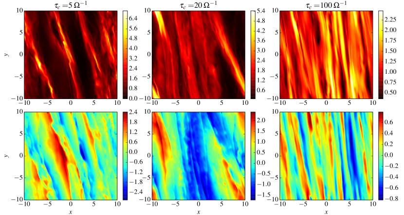
Figure 1: Hydrodynamic gravito-turbulent states used as initial conditions for the dynamo problem. The colourmaps represent gas density $\rho$ (top) and radial velocity $u_{x}$ (bottom) in the midplane $z=0$. From left to right, $\tau_{c}=5,20$ and $100\,\Omega^{-1}$.

2.4.1 Averages

To analyse the statistical behaviour of the turbulent flow, we define the standard and weighted box averages

$$\left<X\right>=\frac{1}{V}\int_{V}X\,\,dV,\quad\text{and}\quad\left<X\right>_{W}=\frac{1}{V\left<\rho\right>}\int_{V}\rho X\,\,dV,$$ (10)

respectively, where $V=L_{x}L_{y}L_{z}$ is the volume of the box. We also define the horizontally averaged vertical profile of a dependent variable:

$$\overline{X}(z)=\dfrac{1}{L_{x}L_{y}}\int\int X\,\,dxdy.$$ (11)

An important quantity is the average 2D Toomre parameter defined by

$$Q_{W}=\dfrac{\left\langle c_{s}\right\rangle_{W}\Omega}{\pi G\Sigma},$$ (12)

where $\Sigma=L_{z}\left<\rho\right>$ is the average surface density of the disc. Another quantity that characterises the turbulent dynamics is the coefficient $\alpha$ which measures the angular momentum transport efficiency. This quantity is the sum of the total stress (which includes gravitational $G_{xy}$, Reynolds $H_{xy}$ and Maxwell stresses $M_{xy}$) divided by the box average pressure:

$$\alpha=\dfrac{\left\langle H_{xy}+G_{xy}+M_{xy}\right\rangle}{\langle P\rangle},$$ (13)

where

$$H_{xy}=\rho u_{x}u_{y},\quad G_{xy}=\dfrac{1}{4\pi G}\dfrac{\partial\Phi}{\partial x}\dfrac{\partial\Phi}{\partial y}\quad\text{and}\quad M_{xy}=-B_{x}B_{y}.$$

Finally, we denote by $E_{c}=\frac{1}{2}\langle\rho\mathbf{u}^{2}\rangle$ and $E_{m}=\frac{1}{2}\langle\mathbf{B}^{2}\rangle$ the box averaged kinetic and magnetic energies.

2.4.2 Fourier modes

To analyse the structure of the magnetic field, we use the 2D Fourier decomposition of these fields in $x$ and $y$. The Fourier modes are calculated as in Riols et al. (2017a) (Section 2.5.2). We denote by $k_{x}$ and $k_{y}$ the radial and azimuthal Eulerian wavenumbers. In this mathematical representation, fields are a sum of a mean ($k_{x}=0$ and $k_{y}=0$) mode, axisymmetric modes with $k_{y}=0$ ($k_{x}\neq 0$), and non-axisymmetric modes with $k_{y}\neq 0$ (commonly referred as “shearing waves"). A large-scale wake or spiral wave can be viewed as the result of the constructive interference of multiple shearing waves of different $k_{x}$ but the same, fundamental, azimuthal wavenumber $k_{y}=2\pi/L_{y}$ (see Ogilvie & Lubow, 2002)

2.4.3 Mean magnetic field and dynamo equation

In Section 4, we investigate the ability of GI to sustain a large-scale dynamo throughout the domain. A key quantity is the mean magnetic field $\overline{\mathbf{B}}(z)$, averaged in the $x$ and $y$ directions, corresponding to the $k_{x}=0$ and $k_{y}=0$ Fourier component of $\mathbf{B}$. The equations governing the horizontally-averaged radial and toroidal fields are:

$$\dfrac{\partial\overline{B}_{x}}{\partial t}=-\dfrac{\partial\mathcal{\overline{E}}_{y}}{\partial z}+\dfrac{1}{\text{Rm}}\dfrac{\partial^{2}{\overline{B}}_{x}}{\partial z^{2}}$$ (14)

$$\dfrac{\partial\overline{B}_{y}}{\partial t}=\ -S\overline{{B}}_{x}+\dfrac{\partial\mathcal{\overline{E}}_{x}}{\partial z}+\dfrac{1}{\text{Rm}}\dfrac{\partial^{2}{\overline{B}}_{y}}{\partial z^{2}}$$ (15)

with $\overline{\mathbfcal{E}}(z)=\overline{\mathbf{u}\times\mathbf{B}}$ the horizontally-averaged electromotive force (EMF). If we denote $\mathbf{\tilde{b}}=\mathbf{B}-\overline{\mathbf{B}}$ and $\tilde{\mathbf{u}}=\mathbf{u}-\overline{\mathbf{u}}$, i.e. perturbations in the magnetic and velocity fields, then we have

$$\overline{\mathbfcal{E}}(z)=\overline{\mathbf{u}}\times\overline{\mathbf{B}}+\overline{\mathbf{\tilde{u}}\times\mathbf{\tilde{b}}}$$ (16)

The first “laminar" term is due to the mean flow, while the second “turbulent’ term issues from the correlation between velocity and magnetic perturbations. We recall that the mean radial and toroidal fields in the box, respectively $\langle B_{x}\rangle$ and $\langle B_{y}\rangle$ (equal to the $z$-average of $\overline{{B}}_{x}(z)$ and $\overline{{B}}_{x}(z)$), are free to vary.

3 GI-dynamo threshold and saturation

In the regime of moderate cooling ($\tau_{c}\gtrsim 3\,\Omega^{-1})$ the GI breaks down into a disordered state, often referred to as “gravito-turbulence", the properties of which have prompted considerable study (Gammie, 2001; Rice et al., 2003; Paardekooper, 2012; Shi & Chiang, 2014; Hirose & Shi, 2017; Riols et al., 2017a). The aim of this section is to determine, for a given Rm and by using numerical simulations, the ability of gravito-turbulent flows to generate magnetic fields. We calculate, in particular, the growth rates and saturated states of the associated dynamo as a function of Rm. We stress that the large resistivity in our simulations prohibits excitation of the MRI, so any field growth cannot be attributed to it.

Run	Resolution	Time (in $\Omega^{-1}$)	$\tau_{c}$	$Q_{W}$	$E_{c}$/$\langle P\rangle$	$\langle H_{xy}\rangle$/$\langle P\rangle$	$\langle G_{xy}\rangle$/$\langle P\rangle$	$\alpha$	$\alpha_{th}=1/(\Omega\tau_{c})$
SGhydro-5	$256\times 256\times 96$	100	5	1.239	0.67	0.063	0.117	0.18	0.2
SGhydro-20	$256\times 256\times 96$	200	20	1.194	0.191	0.0132	0.0345	0.048	0.05
SGhydro-100	$256\times 256\times 96$	400	100	1.29	0.088	0.0032	0.00804	0.011	0.01

Table 1: Parameters and properties of hydrodynamical runs in a box of $L_{x}=L_{y}=20H_{0}$. The third columm indicates the time of the simulation over which quantities have been averaged. $Q_{W}$ is the (density weighted) average Toomre parameter, $E_{c}/\langle P\rangle$ is the ratio of box-averaged kinetic energy over pressure, $H_{xy}$, $G_{xy}$ and $\alpha$ are the averaged Reynolds, gravitational stress, and angular momentum transport, respectively.

3.1 Hydrodynamic flows

Numerically, the usual way to study dynamos in turbulent flows is to start from the hydrodynamic state of fully-developed turbulence, and then introduce a magnetic seed to see whether it grows or decays over time. To prepare the initial states, we ran a set of pure hydrodynamic GI simulations, as in Riols et al. (2017a), with moderate resolution (13 points per $H_{0}$ in the horizontal directions and 16 points in the vertical). This resolution allows us to resolve magnetic Reynolds number up to 200 (see Section 2.3).

As described in Riols et al. (2017a) the strength and saturation of the gravito-turbulence is set by the cooling time $\tau_{c}$. In particular, the time-averaged stress to pressure ratio follows the Gammie (2001) relation:

$$\alpha\simeq\dfrac{1}{q\Omega(\gamma-1)\tau_{c}}=\dfrac{1}{\Omega\tau_{c}}\quad(\gamma=5/3,\,q=3/2)$$ (17)

Three different $\tau_{c}$ have been considered: $\tau_{c}=5\,\Omega^{-1}$ (strong turbulence, close to the fragmentation threshold), $\tau_{c}=20\,\Omega^{-1}$ (moderate turbulence) and $\tau_{c}=100\,\Omega^{-1}$ (weak turbulence).

Table 1 shows some box and time-averaged quantities for the three different hydrodynamical simulations. While the Toomre parameter varies slightly between simulations, kinetic energy, Reynolds and gravitational stress increase significantly when $\tau_{c}$ decreases. We checked also that the Gammie relation (Eq. 17) holds in the three cases.

Figure 1 shows the density and radial velocity of the turbulent state associated with each $\tau_{c}$. These representative snapshots are chosen at a random time and serve as initial conditions for the dynamo simulations in the next sections. For $\tau_{c}=5\,\Omega^{-1}$ and $\tau_{c}=20\,\Omega^{-1}$, the turbulence is supersonic, highly compressible, and characterized by large-scale spiral density waves, particularly strong in the case $\tau_{c}=5\,\Omega^{-1}$. Small-scale motions, potentially driven by a parametric instability (see Riols et al., 2017a) faintly distort the spiral waves at higher altitude, around $z\simeq H_{0}$. They are also marginally visible in the midplane (Fig .1) but with weaker amplitude. Note that the resolution used here allows us to capture only the largest scales of the parametric instability. In the case $\tau_{c}=100\,\Omega^{-1}$, the flow looks very different: the turbulence is subsonic, the waves are fainter, smoother and thinner, and their pitch angle much smaller.

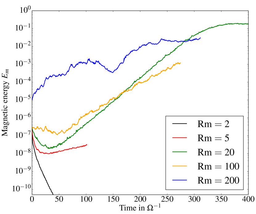
Figure 2: Time evolution of the averaged magnetic energy for different Rm and for $\tau_{c}=20\,\Omega^{-1}$. The initial condition corresponds to the hydrodynamic state shown in Fig. 1 (second column).

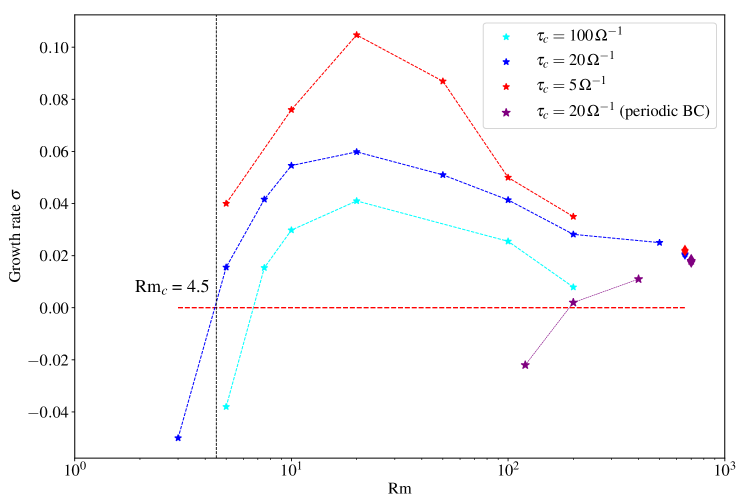
Figure 3: Linear growth rates of the magnetic energy as a function of Rm for 3 different cooling times, $\tau_{c}=5\,\Omega^{-1}$ (red curve), $\tau_{c}=20\,\Omega^{-1}$ (blue curve) and $\tau_{c}=100\,\Omega^{-1}$ (cyan curve). The purple curve is for $\tau_{c}=20\,\Omega^{-1}$ but with periodic boundary conditions. For a given $\tau_{c}$, the initial condition and initial seed magnetic field are identical for all Rm (the initial amplitude is different in the case $\tau_{c}=20\Omega^{-1}$, $\text{Rm}=200$ only). The blue and red diamond markers indicate the growth rate of magnetic energy obtained in the simulations SGMRI-20 and SGMRI-5 of RL18a, respectively, without explicit resistivity and grid $\text{Rm}\sim 660.$

3.2 Kinematic regime and growth rates

Having constructed the hydrodynamic GI turbulent states, we now investigate their amplification of magnetic fields. For a given $\tau_{c}$, we run a series of MHD simulations at different Rm. The initial condition corresponds to the state described in Fig. 1. The magnetic seed introduced at the beginning of the simulations is zero-net flux, toroidal, and has a sinusoidal dependence in $z$. In all cases (except for $\text{Rm}=200$), its amplitude is fixed to $10^{-3}$, which corresponds to an initial $E_{m}=2.5\times 10^{-7}$. This very small value ensures that the Lorentz force has little effect on the gas dynamics during the first few hundred $\Omega^{-1}$, at least on large scales, and thus any dynamo action is purely kinematic.

We first analyse the intermediate cooling regime with $\tau_{c}=20\,\Omega^{-1}$. Figure 2 shows the time evolution of the box-averaged magnetic energy $E_{m}$ for different Rm. For $\text{Rm}=2$, we found that the magnetic energy falls to 0 with decay rate close to 0.14$\Omega$. For Rm between 5 and 100, $E_{m}$ evolves quasi-exponentially with a well-defined growth rate. This is particularly striking in the case of $\text{Rm}=20$ (green curve) for which a clean exponential amplification is obtained for at least $300\,\Omega^{-1}$. Saturation of magnetic energy occurs after this point (a regime analysed in Section 3.3).

For the largest Rm shown in the figure ($\text{Rm}=200$, blue curve), we found that the magnetic field is amplified with growth rate $\sigma\sim 0.028\Omega$, measured by fitting an exponential curve to the numerical data. Unlike the more resistive cases we explored, its evolution is more complex than a simple exponential growth; the field exhibits intermittent bursts with long periods of about $100\,\Omega^{-1}$ and shorter periods of $\sim 10\,\Omega^{-1}$. We checked that the same behaviour is obtained when $\text{Rm}=500$ with double the resolution. Unsurprisingly perhaps, it resembles the dynamo identified by RL18a in the limit of ideal MHD (without explicit resistivity). We are hence tempted to conclude that the simulations are only marginally resolved at this Rm. What we may be seeing is the grid (rather than explicit resistivity) beginning to control the dynamics.

We collect the growth rates obtained from all simulations with cooling time $\tau_{c}=20\,\Omega^{-1}$ and plot their dependence on Rm in Figure 3 (blue curve). To make a comparison with the ideal limit, we also show in this diagram the growth rate measured in the simulation SGMRI-20 of RL18a which had no explicit resistivity (blue diamond marker). We deduce from this figure that the critical threshold for the dynamo is $\text{Rm}\gtrsim 4-5$. Its growth rate is maximal for $\text{Rm}\simeq 20$ (with $\sigma_{max}\simeq 0.06\Omega$) and decreases at larger Rm.

In addition, we explore the dependence of the growth rates on $\tau_{c}$, by repeating exactly the same procedure as described above, for $\tau_{c}=100\,\Omega^{-1}$ and $\tau_{c}=5\,\Omega^{-1}$. The corresponding growth rates are superimposed on Fig. 3 to make direct comparison with $\tau_{c}=20\,\Omega^{-1}$. In the case of inefficient cooling (cyan curve, $\tau_{c}=100\,\Omega^{-1}$), the dynamo is still active and the dependence on Rm is very similar to $\tau_{c}=20\,\Omega^{-1}$. However, the growth rates are lower and reduced by a factor 1.5$-$2. For efficient cooling (red curve, $\tau_{c}=5\,\Omega^{-1}$), turbulent motions are stronger and growth rates are consequently larger. The maximum amplification occurs again for $\text{Rm}\simeq 20$, with growth rate $\sigma\simeq 0.1\Omega$. In this regime magnetic fields are efficiently amplified so that they reach a quasi-steady configuration within a few orbits.

To summarize, GI can amplify a magnetic field for a wide range of $\tau_{c}$ and the dynamo persists at very small $\text{Rm}\gtrsim 4$. In addition to its kinematic and linear properties, we demonstrate that the dynamo behaves like a “slow" dynamo, with growth rates decreasing with increasing Rm above a critical value. The runs at double resolution with $\text{Rm}=500$ and those without explicit resistivity (grid Rm $\simeq H/\Delta_{x}^{2}\simeq$ 660) suggest perhaps that the growth rate decreases more slowly at higher Rm, indicative of a different dynamo regime. Despite this trend, we emphasize that predicting the dynamo behaviour at larger Rm or in the ideal limit remains extremely difficult. Testing the convergence of the dynamo growth rate with Rm would require us to go beyond $\text{Rm}\sim 1000$, which is inaccessible with our current resources. In any case, these results suggest that ohmic diffusion is crucial for the maintenance of a powerful and efficient dynamo.

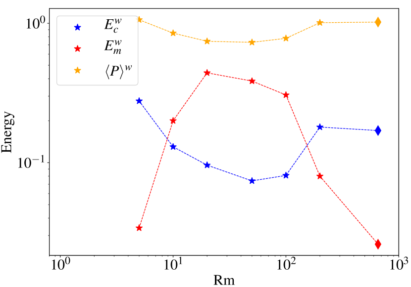
Figure 4: Pressure, kinetic and magnetic energy as a function of Rm for $\tau_{c}=20\,\Omega^{-1}$ during the quasi-steady nonlinear regime. Quantities are weighted by the gas density and averaged over the box and. The diamond markers correspond to the simulation without explicit resistivity with grid $\text{Rm}\sim 660$.

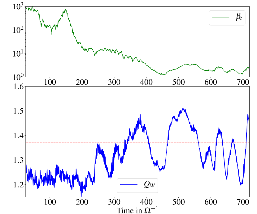
Figure 5: Time-evolution of turbulent beta plasma $\beta_{t}$ (top) and Toomre parameter (bottom) for $\text{Rm}=50$ and $\tau_{c}=20\,\Omega^{-1}$. Quantities are averaged over the box with density weighting.

3.3 Saturation and nonlinear regime

We now explore the non-linear regime of the dynamo, i.e when the Lorentz force provides feedback on the turbulent flow. What is the dependence of the saturated state on Rm and how strongly does resistivity affect GI turbulence?

First, we plot in Fig. 4 the box-averaged pressure, kinetic and magnetic energy obtained in the saturated state (when the magnetic field stops growing) as a function of Rm and for $\tau_{c}=20\,\Omega^{-1}$. Since the field concentrates within the bulk of the disc (see Section 4.1), we weighted quantities by the gas density during the averaging procedure. We see that the saturated magnetic energy in the nonlinear regime depends on the parameters in the same way as the kinematic growth rates (see Fig. 3 for comparison). $E_{m}$ is maximal for $\text{Rm}\ \sim 20$ and decreases quite abruptly towards $\text{Rm}\gtrsim 200$. At its maximum, the dynamo sustains strong magnetic fields with a plasma beta $\beta_{t}=\langle P\rangle/E_{m}\sim 2$ and energy typically 5-6 times larger than the turbulent kinetic energy in the bulk of the disc. This corresponds to a regime of super-equipartition fields, for which we expect important feedback of the Lorentz force on the gas flow. For Rm between 10 and 100, the kinetic energy is reduced by a factor almost 3 compared to the ideal limit and by a factor 6 compared to the unmagnetized gravitoturbulence. We checked that the gravitational stress is also reduced in this regime.

In RL18a, we showed that ideal-MHD gravitoturbulence exhibits a moderate drop in kinetic energy in comparison to the purely hydrodynamical case, a property attributed to the non-linear suppression of large-scale structures, such as oscillatory epicyclic modes. In the low Rm regime, the drop in kinetic energy is more dramatic because of the stronger magnetic field. Additional effects, associated with magnetic pressure and thermodynamics, may also contribute; for instance, since the kinetic to magnetic pressure ratio is of order unity for Rm between 10 and 100, the linear stability and growth rate of spiral GI modes will be altered. Indeed, the effective Toomre parameter, including magnetic pressure, is

$$Q_{\text{eff}}\approx Q_{\text{hydro}}\sqrt{1+\dfrac{1}{\beta_{t}}}$$ (18)

(Kim & Ostriker, 2001) which is $25\%$ greater than the hydrodynamic $Q$ in the low Rm states. Moreover, magnetic fields provide an additional reservoir of energy that can be directed into ohmic heating and, consequently, an enhanced $Q$.

To study this effect, we plot in Fig. 5 the evolution of the box-average Toomre parameter $Q_{W}$ as a function of time for $\text{Rm}=50$. In the initial state and during the kinematic phase, the magnetic field is too small to influence the flow and $Q_{W}$ settles around its hydrodynamical value ($Q_{W}\simeq 1.2$). In the final state, with $\beta_{t}\approx 2$, the average Toomre parameter is $Q_{W}\simeq 1.37$. Therefore there is an increase of almost 15% (and equivalently of the average sound speed in the midplane). Note however that the elevation of disc temperature remains moderate, despite the strong magnetization. In particular, it is relatively small compared to that measured in a 2D disk (Riols & Latter, 2016). Nonetheless, by combining the effect of magnetic pressure and ohmic dissipation, the effective $Q$ in the low Rm regime can be 40% higher than in pure hydrodynamics, leading to fainter spiral waves and a depression of GI activity.

Interestingly, $Q$ exhibits notable oscillations when the magnetization becomes important (at $t=300\,\Omega^{-1}$). These oscillations must reflect the back-reaction of the field on the flow. They probably originate from a thermal cycle similar to that described in RL18a (Section 5.4), in which (a) GI amplifies $\mathbf{B}$, (b) magnetic energy is dissipated into heat and enhances $Q$, (c) GI or spiral activity dies because of the high $Q$ and strong magnetic tension, and finally (d) in the absence of vigorous GI, $\mathbf{B}$ and $Q$ return to their original value. This scenario is consistent with the fact that the variations of $Q$ and $\beta_{t}$ in Fig. 5 are correlated.

The dependence of saturated state on cooling times was explored in RL18a in the ideal limit. In the case of finite resistivity, we find that magnetic energy also peaks around $\text{Rm}=20$ for $\tau_{c}=100\,\Omega^{-1}$. However for $\tau_{c}=5\Omega^{-1}$, simulations have not been run for sufficiently long time to be statistically meaningful. The reason is that most stalled after a few tens of an orbit because of transient fragments that considerably reduce the time step.

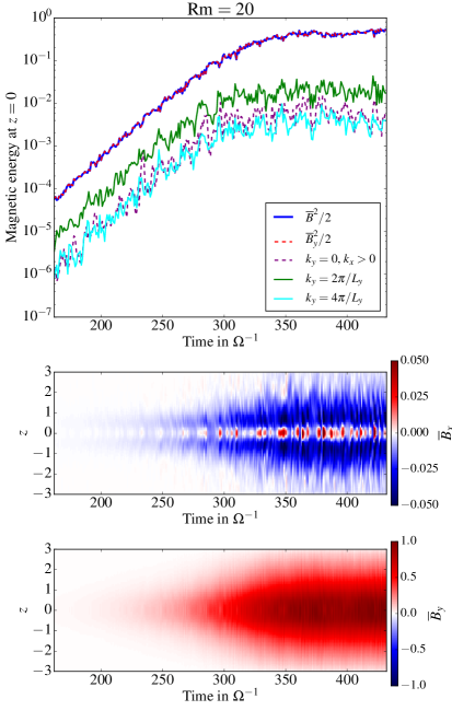
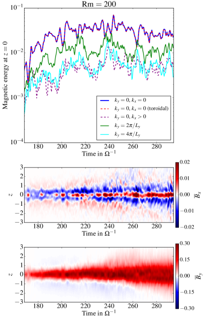
Figure 6: Top: time evolution of magnetic energy contained within the midplane ($z=0$), projected onto different Fourier components, for $\tau_{c}=20\,\Omega^{-1}$. Blue/solid lines correspond to the total magnetic energy and red/dashed lines to the total toroidal field $B_{y}$. Purple/dashed lines represent the magnetic energy projected onto the axisymmetric modes ($k_{x}\neq 0$, $k_{y}=0$). Green and cyan plain lines correspond to the energy of non-axisymmetric components, respectively $k_{y}=2\pi/L_{y}$ and $k_{y}=4\pi/L_{y}$. Lower panels: space-time $(t,z)$ diagram of the mean $\overline{B}_{x}$ and $\overline{B}_{y}$. The left panels are for $\text{Rm}=20$ and the right panels are for $\text{Rm}=200$.

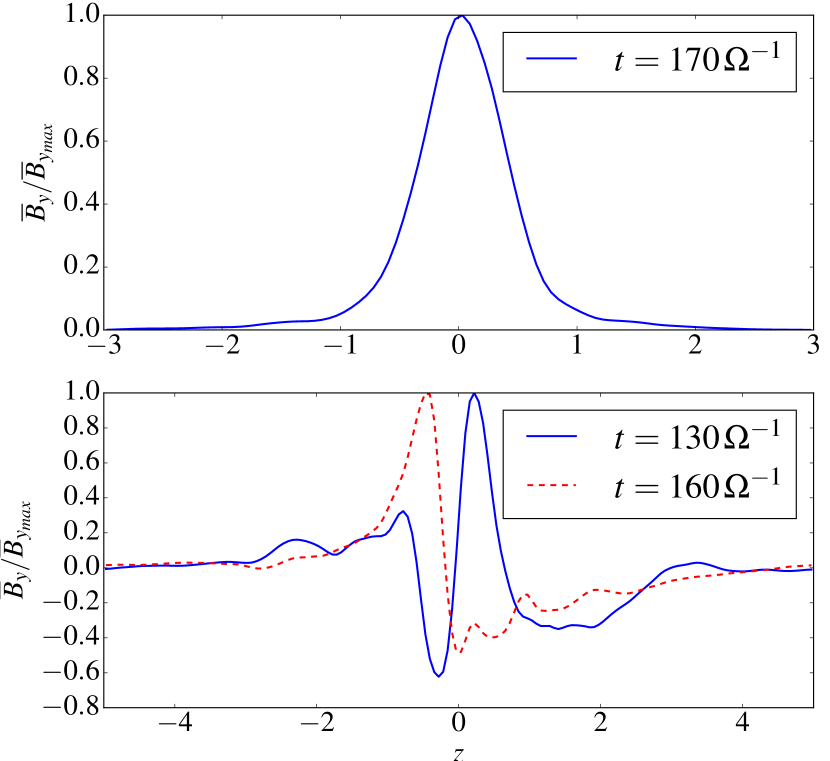
Figure 7: Vertical profile of $\overline{B}_{y}$ for $\text{Rm}=200$, with open boundaries (top) and periodic boundaries (bottom). In the latter case, two different times are represented to show the flipping of $\overline{B}_{y}$.

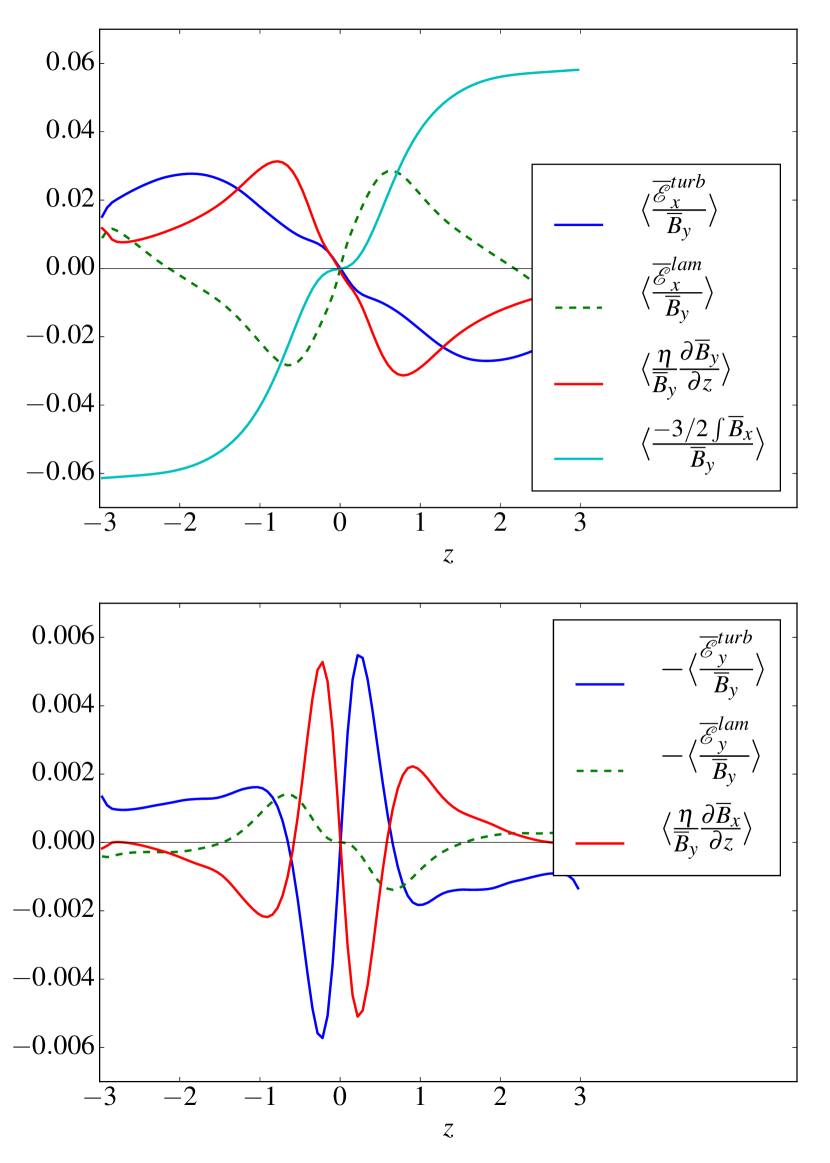
Figure 8: Vertical profiles of the electromotive forces, ohmic current and linear stretching term (omega effect) involved in the evolution of $\overline{B}_{y}$ (top) and $\overline{B}_{x}$ (bottom), for $\text{Rm}=20$, $\tau_{c}=20\,\Omega^{-1}$ and open boundaries. We remind the reader that $\mathcal{\overline{E}}^{lam}(z)=\overline{\mathbf{u}}\times\overline{\mathbf{B}}$ and $\mathcal{\overline{E}}^{turb}(z)=\overline{\mathbf{\tilde{u}}\times\mathbf{\tilde{b}}}$. All terms are normalized to the midplane $\overline{B}_{y}$ and averaged over $x$, $y$ and time, during the kinematic phase.

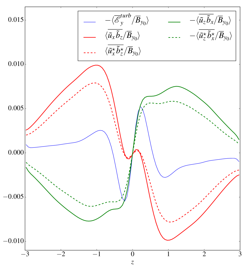
Figure 9: Vertical profiles of the toroidal EMF $\mathcal{\overline{E}}_{y}$ (blue line) and contribution of horizontal (red lines) and vertical (green lines) motions to $\mathcal{\overline{E}}_{y}$. The dashed lines are the EMF calculated by filtering out small-scale non-axisymmetric perturbations in Fourier space and retaining only the modes with $k_{y}\leq 2\pi/L_{y}$. All terms are normalized to the midplane $\overline{B}_{y}$ and averaged over $x$, $y$ and time, during the kinematic phase.

3.4 Dependence on boundary conditions

In the solar context, boundary conditions strongly influence the excitation and saturation of convective dynamos (e. g. Choudhuri, 1984; Jouve et al., 2008; Käpylä et al., 2010). We now check if the GI dynamo exhibits a similar sensitivity. We compared three different vertical boundaries: vertical field (open boundary), perfect conductor (closed boundary), and periodic. Note that the perfect conductor has $u_{z}=0$, $B_{z}=0$ and $dB_{x}/dz=dB_{y}/dz=0$. In theory, it prevents any EMF from being generated at the boundary or outside the domain, and conserves magnetic helicity in the box. However, in practice, given that the EMF is reconstructed at the cell interfaces while boundaries are given at cells centres, the code still generates a non-vanishing EMF at the boundary that can lead to a mean $\langle B_{x}\rangle$ and $\langle B_{y}\rangle$. When using such condition, we found similar dynamo growth rates as in the open boundaries case, but ended up with higher magnetization in the saturated state.

Periodic boundary conditions are interesting since they ensure that no EMF is produced at the boundaries and thus provide the best set-up to test dynamo action as formally defined. We superimpose in Fig. 3 the growth rates obtained for three different Rm (120, 200, 400) and also without explicit diffusion (diamond markers). Although a dynamo appears, the critical magnetic Reynolds number is shifted to higher Rm, with $\text{Rm}_{c}\simeq 200$. Note that this effect appears to be independent of vertical box size because we obtain a similar result with $L_{z}=6H$ and $L_{z}=10H$. As in the open boundary case, the field grows quasi-exponentially, but growth rates and saturated magnetic energy are lower. The fact that the dynamo depends strongly on the nature of the boundary is actually not surprising. We will show in Section 4.2 that periodic boundaries prevent flux from leaving the domain and even to be recycled from the upper surface to the lower surface (and vice versa), which is somewhat unrealistic. One quantifiable effect is that the large-scale magnetic field is forced to be antisymmetric about the midplane, which enhances ohmic diffusion.

4 Dynamo properties

In this section we turn our attention from the dynamo’s broad-brush features (growth rates, saturated amplitudes) and concentrate on some of its specifics so as to better understand how it works. We focus primarily on the kinematic phase of its evolution.

4.1 Large or small scale?

To understand whether the GI-dynamo preferentially amplifies large or small-scale fields, we show in Fig. 6 (top panels) the evolution of magnetic energy associated with different Fourier modes when $\tau_{c}=20\Omega^{-1}$. The calculation is restricted to the midplane $z=0$ as it contains most of the magnetic energy. For both $\text{Rm}=20$ and $\text{Rm}=200$, the magnetic field is clearly dominated by the mean component $\overline{\mathbf{B}}$ ($k_{x}=0$, $k_{y}=0$), and especially its toroidal projection $\overline{B}_{y}$. The dynamo is thus predominantly large scale, in the sense that magnetic fields grow on lengths much larger than $H$.

The second important component is the fundamental non-axisymmetric mode $k_{y}=2\pi/L_{y}$ (in green) which corresponds to a large scale spiral magnetic structure (see section 5). Non-axisymmetric modes are essential to the dynamo process according to the Cowling’s anti-dynamo theorem, so we expect them to feature. In particular, the interaction of their magnetic and velocity components produce a mean electromotive force that allows $\overline{\mathbf{B}}$ to be constantly re-generated so as to compensate ohmic losses. Note that axisymmetric modes with $k_{y}=0$ and $k_{x}>0$ seem negligible in the magnetic energy budget.

Cases $\text{Rm}=20$ and $\text{Rm}=200$ are distinguished by their ratio of large to small scale magnetic fields. In terms of energy, there is only a factor 4 difference between the mean $\overline{B}_{y}$ and the non-axisymmetric harmonic $k_{y}=4\pi/L_{y}$ for $\text{Rm}=200$, while this ratio exceeds 100 when $\text{Rm}=20$. This we attribute to a drop in the mean field $\overline{\mathbf{B}}$, the saturation level of the non-axisymmetric mode being unchanged when Rm is increased. So it would appear that the large-scale dynamo is weakened at large Rm, and supplanted by a smaller-scale dynamics. The origin of the small-scale magnetic fields is unclear at this stage. They might originate in a turbulent cascade of magnetic energy, possibly from local magnetic instabilites, or from a small-scale dynamo of Zel’dovich type that stretches and folds the field lines in a random way. The mechanism behind the development of the small-scale field is discussed in Section 5.3. We stress that the MRI is not (or marginally) active in the very diffusive regime considered in this paper, and is anyway likely to be strongly impeded by GI (see RL18a, ).

4.2 Vertical profile of mean magnetic field

In this subsection, we look in more detail at the properties of the large-scale dynamo during its kinematic phase. The lower panels of Fig. 6 show the time-evolution of the vertical profiles of the mean magnetic field $\overline{B}_{x}(z)$ (center) and $\overline{B}_{y}(z)$ (bottom) for $\tau_{c}=20\,\Omega^{-1}$ and open boundary conditions. For both $\text{Rm}=20$ and $\text{Rm}=200$, the large-scale field is mainly toroidal $\overline{B}_{y}/\overline{B}_{x}\simeq 20$ and remains confined within the midplane region of the disc. This is reminiscent of simulations without explicit resistivity (RL18a). Unlike the latter, however, the dynamo in resistive flow does not exhibit time-reversals of $\overline{\mathbf{B}}$, or possibly these reversals occur on timescales longer than $400\,\Omega^{-1}$. Figure 6 shows that both poloidal and toroidal components have the same polarity in the midplane, but $\overline{B}_{x}$ changes its sign at $z\simeq 0.2-0.3H$. For $\text{Rm}=20$, the diagram also reveals bursts of poloidal field confined to the midplane. These bursts are correlated with the activity of vigorous density spiral waves. We note finally that for large Rm, both the radial and toroidal mean field almost vanish in the disc atmosphere, above one disc scaleheight.

Figure 7 compares the vertical profile of $\overline{B}_{y}(z)$ produced from simulations with open and with periodic boundary conditions, for $\text{Rm}=200$. Each profile is calculated at a given time of the simulation during the kinematic phase. In the case of periodic boundaries, the field is antisymmetric about the midplane, with a different polarity in the upper and lower parts of the disc. This configuration ensures that the mean $B_{x}$ and $B_{y}$ vanish in the box, but not over each side of the disc. Therefore, the large-scale field in a periodic box corresponds to the $n=1$ mode in $z$ (instead of $n=0$ for open boundaries) which possesses a strong gradient at $z=0$. The vertical scale associated with this gradient can be measured from Fig. 7 and is $\Delta z\simeq 0.2H$. In comparison the vertical scale of $\overline{B}_{y}(z)$ in open boundaries simulations is 5 to 6 times larger. As a consequence, ohmic diffusion on $\overline{B}_{y}$ is enhanced by a factor of a few tens, which should enhance the critical magnetic Reynolds number of the dynamo. In addition, horizontally averaged fields $\overline{B}_{x}$ and $\overline{B}_{y}$ did not necessarily dominate the magnetic energy budget and flipped regularly in time, with a short period of 5-6 orbits (see Fig. 7).

4.3 Electromagnetic forces

We now investigate how the mean field is regenerated. We focus particularly on the simulation with open boundaries, $\tau_{c}=20\,\Omega^{-1}$ and $\text{Rm}=20$. In Fig. 8, we plot the vertical profiles of the different terms in Eq. (14) and Eq. (15) governing the evolution of $\mathbf{\overline{B}}$. This includes the laminar and turbulent part of the mean electromotive force $\overline{\mathbf{u}\times\mathbf{B}}$, as well as the shear stretching (the “omega effect”) and ohmic diffusion $\eta\mathbf{\overline{J}}$. All these terms are averaged in time, during the kinematic phase (between $t=150$ and $t=350\,\Omega^{-1}$), and over the horizontal plane. Since their evolution is exponential during the amplification phase, we normalize them by the midplane $\overline{B}_{y_{0}}$ during the averaging procedure.

The top panel shows that the toroidal component $\overline{B}_{y}>0$ is mainly amplified via the radial laminar EMF (green dashed curve) and the omega effect (cyan), since both have a positive gradient in $z$. In contrast, the radial turbulent EMF (blue) has a negative gradient in $z$, like ohmic diffusion (red), and therefore acts as a turbulent diffusion on the mean field. Note that the radial laminar EMF $\simeq-\overline{u}_{z}\overline{B}_{y}$ is associated with compression of the disc due to a mean inflow $v_{z}\simeq-0.04\,|z|<0$. This inflow remains relatively weak compared to the r.m.s vertical velocity and is confined to the midplane regions $|z|\lesssim 1H$. Further away in the disc corona, $v_{z}$ is now positive and expels magnetic flux outward. Although the EMF generated by the inflow near $z=0$ is comparable to the stretching by the shear (omega effect), it is insufficient on its own to sustain the toroidal field against ohmic and turbulent diffusion. The omega effect is essential, and so we conclude that a poloidal field is required for the large-scale dynamo to work.

The bottom panel shows the EMFs and ohmic diffusion profiles associated with the radial field $\overline{B}_{x}$. Here the laminar term (dashed green curve) is almost negligible compared to the turbulent EMF (blue). Moreover, the profiles are more complicated in the bulk of the disk $|z|<H$. We point out that the toroidal and turbulent EMF $\mathcal{\overline{E}}_{y}$ has two local extrema of opposite signs, one around $z\simeq 0.3H$ and one around $z\simeq 1-1.5H$. These extrema correspond to a change in the sign of the EMF gradient, and then to a change of $\overline{B}_{x}$ polarity (see Fig. 6 for comparison). Since both are correlated and keep the same sign, the turbulent EMF $\mathcal{\overline{E}}_{y}$ is directly involved in the maintenance of the mean radial field against ohmic diffusion.

4.4 Nature of turbulent motions involved in $\mathcal{\overline{E}}^{turb}_{y}$

To proceed further in the analysis we need to understand the turbulent EMF. In Fig. 9 we plot the part of the mean EMF $-\mathcal{\overline{E}}^{turb}_{y}$ that issues from radial motions $\overline{\tilde{u}_{x}\tilde{b}_{z}}$ (red curve) and the part that issues from vertical motions $-\overline{\tilde{u}_{z}\tilde{b}_{x}}$ (green). In the midplane ($|z|\lesssim 0.3H$) where $B_{x}B_{y}>0$, the EMF is entirely due to vertical motions (such as upwellings and rolls). In particular, this means that the strong horizontal motions associated with spiral waves do not play a direct role in the regeneration of the mean poloidal field (though they play an indirect role, see Section 5). Higher up, in the disc corona, both radial and vertical motions contribute to the EMF, with $\overline{\tilde{u}_{x}\tilde{b}_{z}}$ being slightly stronger and leading to the change of $\overline{B}_{x}$ polarity.

To determine whether the mean field is generated by large-scale motions (like spiral waves) or small-scale fluctuations, we calculate the contribution of large-scale modes with $k_{y}\leq 2\pi/L_{y}$ to the EMF. In practice, this is done by computing the direct FFT of $\tilde{u}_{x}$, $\tilde{u}_{z}$, $\tilde{b}_{x}$ and $\tilde{b}_{y}$, filtering out all the Fourier modes that have $k_{y}>2\pi/L_{y}$, and then going back to real space to calculate the products $\tilde{u}^{\star}_{x}\tilde{b}^{\star}_{z}$ and $\tilde{u}^{\star}_{z}\tilde{b}^{\star}_{x}$, where ^⋆ refers to a filtered component. This procedure removes the correlation associated with small-scale non-axisymmetric turbulent structures, such as helical waves generated by parametric instability, for instance (Riols et al., 2017a). We superimpose in Fig. 9 the filtered EMF (dashed lines) and show that they represent approximately 80% of the total EMF. This is strong evidence that the mean field dynamo is supplied by motions associated with large scale spiral waves (with $k_{y}=2\pi/L_{y}$ and radial size $\lambda\simeq H$) rather than GI small-scale turbulence.

In summary, we have demonstrated that the dynamo functions via (a) the creation of $B_{y}$ from $B_{x}$ by the omega effect (mainly) and (b) generation of $B_{x}$ by relatively large-scale, but turbulent, velocity fluctuations issuing from the spiral density waves.

4.5 Mean field theory and its limitations

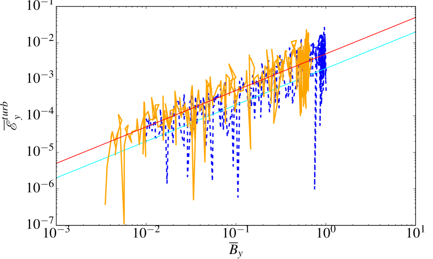
Figure 10: Phase portrait of the mean turbulent EMF $|\mathcal{\overline{E}}_{y}|$ versus the mean toroidal field $\overline{B}_{y}$, during the whole simulation time, for $\tau_{c}=20\,\Omega^{-1}$ and $\text{Rm}=20$. The blue line is the EMF at $z=0.27H$ (where it is maximum) and the orange line is at $z=H$ (where it is minimum). The dashed line corresponds to negative $\mathcal{\overline{E}}_{y}$ while the plain line corresponds to positive $\mathcal{\overline{E}}_{y}$. The red and cyan straight lines have respectively equations $y=0.005x$ and $y=-0.002x$.

Figure 10 shows the evolution of the mean turbulent EMF $\mathcal{\overline{E}}_{y}$ as a function of the mean toroidal field $\overline{B}_{y}$, during the course of the simulation with $\text{Rm}=20$, $\tau_{c}=20\,\Omega^{-1}$ and open boundaries. Although the EMF is highly fluctuating in time, on the average it scales linearly with $\overline{B}_{y}$:

$$\mathcal{\overline{E}}_{y}(z)\simeq\alpha_{\text{dyn}}(z)\overline{B}_{y}(z).$$ (19)

with $\alpha_{\text{dyn}}$ of order -0.002 for $z\simeq 0.3H$ and 0.005 for $z\simeq H$. It is hence tempting to describe the dynamo process in the framework of classical mean field theory (Moffatt, 1977; Parker, 1979; Krause & Raedler, 1980; Brandenburg & Subramanian, 2005; Brandenburg, 2018), according to which the mean EMF is assumed to be a linear combination of the mean $\mathbf{\overline{B}}$ and its vertical gradient. The coefficients of the linear system encapsulate the properties of the turbulence and can be derived using the so-called “test field method". However, there are several caveats. First, this theory only applies when $\text{Rm}\ll 1$ or when there is a clear separation of scales between the turbulent motions and the large-scale field. In our simulations, these assumptions are far from satisfied, since the fundamental non-axisymmetric mode associated with spiral arms represents 80% of the mean EMF (see 4.4). Second, we showed that as the EMF changes its sign with altitude, so does $\alpha_{\text{dyn}}$. Mean field theory predicts that $\alpha_{\text{dyn}}$ is proportional to the mean helicity of the flow $\langle\overline{\mathbf{u}\cdot\nabla\times\mathbf{u}}\rangle$, but according to our simulations, the helicity keeps a constant sign on each side of the disc and is therefore not correlated with $\alpha_{\text{dyn}}$. One could probably find a more sophisticated model than Eq. (19) , involving non-diagonal terms and dependences on the mean field gradient, but this is not the object of the paper.

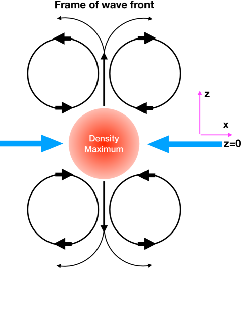
Figure 11: Sketch of the poloidal motions around a spiral density wave in the plane perpendicular to the wavefront. The structure is invariant along the wave front, which has some pitch angle with the azimuthal direction $\mathbf{e}_{y}$. The blue arrows illustrate the horizontal 2D compressible motions, the black arrows the incompressible motions associated with the vertical rolls identified in RL18b. The structure is embedded in a background shear flow coming out of the plane (but with some pitch angle). Such rolls flow is reminiscent of the Roberts flow (Roberts, 1972).

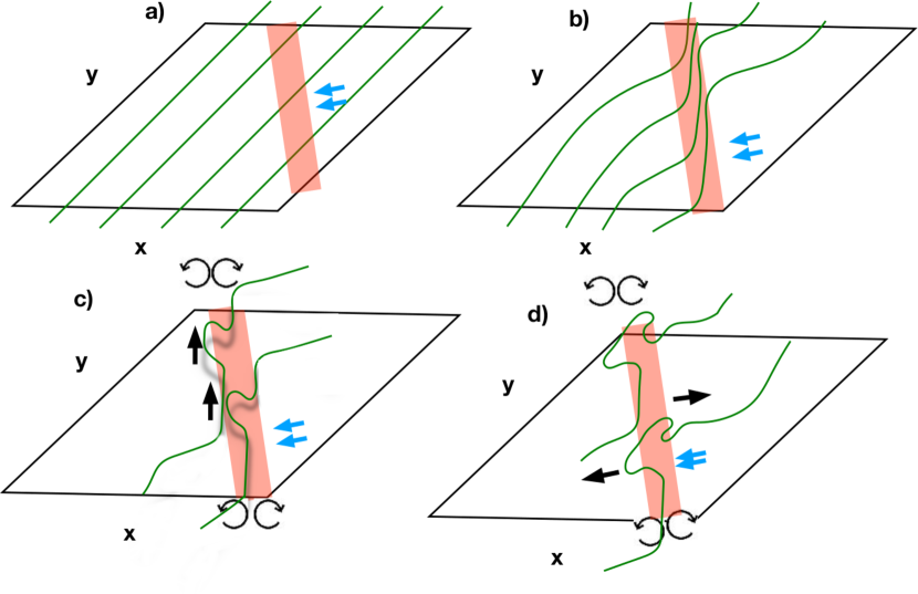
Figure 12: Sketch of the spiral dynamo mechanism. The magnetic field lines are represented in green while the red bar symbolizes a spiral wave. Black arrows denotes the direction in which magnetic field is stretched by the rolls. Each step is described in Section 5.1.

5 Field amplification by density spiral waves: physical picture

We showed in the previous section that the GI efficiently generates and sustains a large-scale magnetic field, especially in the regime of low Rm $\lesssim 100$. This dynamo survives at larger Rm, independently of the vertical boundary condition, but produces weaker mean fields and seems to favour smaller scales. Our aim in this section is to propose a physical picture of the dynamo action, drawing together the different results of the previous sections and providing additional numerical evidence to illustrate the picture.

5.1 Model of the large scale dynamo loop

Our interpretation of the dynamo loop is very similar to the “$\alpha$-$\Omega$" mechanism proposed for the solar dynamo cycle (Parker, 1955). As we showed earlier in Section 4.2, the toroidal field is regenerated from poloidal field, through an omega effect. This is straightforward and uncontroversial. The poloidal field, however, issues from an “alpha" effect supported by large-scale GI spiral motions that stretch and fold the toroidal field. Our task is then to elucidate how the “stretching" and “folding" motions occur, how they amplify $\overline{B}_{x}$, and how these motions connect to the vertical EMF profiles of Section 4.4.

Although the dynamo is a “statistical” effect comprising the work of multiple spiral modes, it is better to start our investigation with a single spiral wave and ask what it does to the magnetic field. For that purpose, we analyse the motion around a simple spiral density wave. Figure 11 sketches out its main dynamical ingredients. The wave is composed of 2D horizontal compressible motions in the midplane (blue arrows) and incompressible vertical roll motions in the poloidal plane (black arrows). These motions are drawn in the frame perpendicular to the wave front, but are actually invariant along the direction of the front. The pattern of four counter-rotating large-scale rolls has been studied in detail by RL18b. These features have a typical size $\simeq H$ and appear as a fundamental feature of linear and nonlinear density waves in stratified discs. They can emerge from a baroclinic effect associated with the thermal stratification of the disc and are generally locally supersonic if the wave is shocked. Such a circulation might also arise from hydraulic jumps in very unstable flows (Boley & Durisen, 2006). Lastly, there is the rotational shear flow coming out of the page, though not perpendicularly. Our pared-down sketch of the spiral wave flow is reminiscent of well-studied and efficient kinematic dynamos such as those of Roberts and Ponamarenko type. It is then perhaps no surprise that we also find dynamo action associated with the density waves.

Note that pure 2D horizontal motions, like those associated with wave compression, are not able to sustain a mean field dynamo on their own. It is true that locally they efficiently produce radial fields, but the mean $\overline{B}_{x}$ induced by these motions (averaged over $x$ and $y$) necessarily vanishes. Thus vertical flow structures, such as the counter-rotating rolls, are essential: this can be seen immediately from the mean toroidal EMF, a large fraction of which is supplied by either vertical motions or vertical magnetic field (see section 4.4).

Putting these ideas together, our interpretation of the dynamo loop, sketched in Fig. 12, is then the following:

1. Initially, the disc is threaded by a pure toroidal field with $B_{y}>0$.

2. A spiral wave, tilted with respect to the azimuthal direction, passes through the disc. The field is then compressed horizontally by the spiral wave, along its pitch angle. On average, this process does not generate any mean radial field: negative $b_{x}$ component is created within the spiral arms, while a positive component is produced outside (in the inter-arm region). See Section 5.2.1 for numerical evidence.

3. Where the field line crosses the centre of the spiral wave, it is pinched and lifted by the vertical velocity associated with the large-scale rolls. This process vertically redistributes the radial field and creates a mean $\overline{B}_{x}$ of opposite polarity in the midplane and in the corona (through the EMF term $\tilde{u}_{z}\tilde{b}_{x}$). See Section 5.2.2 for numerical evidence. A key point here is that the field in the wave isn’t perfectly aligned with the spiral front. Because of this non-alignment, the field lines can be pulled apart by the two different rolls on each side of the wave.

4. As the rolls “turn over" above the disk, they horizontally stretch and fold the field, producing a net $\overline{B}_{x}$ with opposite sign to $B_{y}$ in the corona (through the EMF term $\tilde{u}_{x}\tilde{b}_{z}$). See Section 5.2.2 for more details.

5. Finally, the mean radial field is stretched by the shear (omega effect) which produces a net toroidal field (not shown in Fig. 12)

Naturally, this theoretical picture remains to be demonstrated or at least validated by numerical simulations. The next sections will focus especially on steps (b), (c) and (d).

5.2 Numerical evidence of the spiral wave dynamo loop

To check that our dynamo model can be applied to GI turbulence, we analyse the magnetic field topology around spiral waves in our GI simulations. All the following plots correspond to times when magnetic energy grows linearly (i.e. in the kinematic phase).

5.2.1 Horizontal compression and magnetic spiral patterns: step (b)

We first study the effect of spiral waves’ horizontal motion on magnetic field in simulations with $\tau_{c}=20\,\Omega^{-1}$. We compare in Fig. 13 the density structures in the midplane (top panels) with the $B_{x}$ structures (center panels), for both $\text{Rm}=20$ and $\text{Rm}=500$. In both cases, the radial magnetic field takes the shape of the density spiral waves and concentrates within these structures. In particular, $B_{x}$ is always negative (as opposed to $B_{y}>0$) within the density maxima, and positive outside the spirals. To complete the analysis, we superimpose the horizontal projection of magnetic fields lines over the $B_{x}$ maps. When $\text{Rm}=20$, the magnetic field is relatively strong and almost aligned with the direction of the wave front inside the arms. Each field line, however, crosses the spiral wave since it has to connect with the inter-arm field at some point (therefore, it is not perfectly aligned with the front).

In the inter-arm regions, the field is weaker and has a component perpendicular to the fronts. This configuration is similar to that illustrated in Fig. 12 b) and results from the squeezing of initially toroidal field by compressible motions within the waves. Because the wave has a positive pitch angle , the field inside is tilted in the same direction which leads to a negative $B_{x}$ (assuming an initially positive toroidal field). In the simulation with $\text{Rm}=500$, which has been run at double resolution, the field appears fragmented and more filamentary. However it is again oriented along the spiral front with negative $B_{x}$ inside the density maximum.

5.2.2 Vertical rolls and step (c) and (d)

As suggested by our model (step c), the vertical rolls surrounding each density wave stretch the field lines vertically. To show this effect numerically, we plot in Fig. 14 (top) the vertical structure of the gravito-turbulent flow in the poloidal plane, at a random time. Around the most prominent density waves, marked by a pink rectangle, we clearly identify a pair of counter-rotating rolls, similar to those depicted in Fig. 11.

The left panels of Fig. 15 show $B_{z}$ (top) and $B_{x}$ (bottom) around one of the rolls. For $z>0$, as the field passes through the spiral wave (from “left" to “right"), it rises upward and produces a positive $\tilde{b}_{z}$ component (shown in red). Once it reaches the centre of the spiral, field lines move back toward the midplane $z=0$ and finally connect with the inter-arm field, leading to a negative $\tilde{b}_{z}$ (shown in blue) on the other side of the wavefront. Counterintuitively, the magnetic field is not wrapped around the centre of each roll, but is simply pinched at the centre of the wave, where the vertical velocity of the roll is maximum, exactly as depicted in Fig. 12 (c).

Ultimately, the field that rises up to $z\simeq H$ is stretched horizontally by the counter-rotating motions of each roll and produces a radial field component in the corona (step d). The stretching leads to a “mushroom-like" structure in the contours of $B_{x}$, reflected on either side of the midplane. These contours are plotted in white in the bottom left panel of Fig. 15.

In order to illustrate this process as cleanly as possible we simulate a simple laminar nonlinear shearing density wave initially embedded in a uniform toroidal field $B_{y_{0}}=0.02$ with $\text{Rm}=20$. The setup is the same as in RL18b: the wave is forced not by the GI but by a potential of the form $\Phi_{\text{ext}}=A\,\cos\left[k_{x}(t)x+mk_{y_{0}}y\right]$ where $A$ is the amplitude of the forcing and $k_{x}(t),k_{y_{0}}=2\pi/L_{y}$ are the radial and azimuthal wavenumbers. We fix the amplitude $A=0.6$ in order to obtain a nonlinear shock wave. The initial pressure profile is polytopic $P=K\rho^{1+1/s}$ with index $s=20$ (to mimic the entropy gradient found in our GI simulations, see RL18b). The spiral wave structure and its magnetic topology are shown in the right panels of Fig.15. The flow exhibits a roll structure, and this generates a cleaner version of the magnetic topology seen in the turbulent case (compare with the left panels). Again the stretching of the field gives rise to a mushroom structure, clearly visible in the bottom right panel of Fig.15.

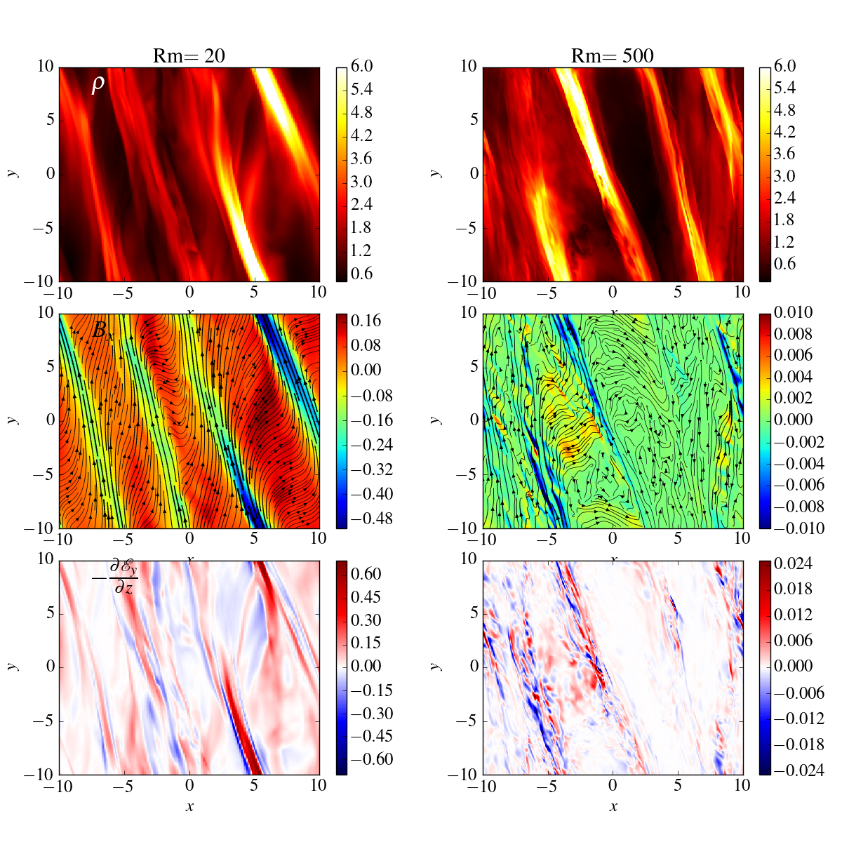
Figure 13: Density and magnetic field structures within the midplane ($z=0$), for $\text{Rm}=20$ (left panels) and $\text{Rm}=500$ (right panels). Snapshots are taken at a random time of the simulation during the linear phase. From top to bottom, $\rho$, $B_{x}$ and the vertical derivative of the toroidal EMF $-\mathcal{E}_{y}$. In the center panels, the arrows are the horizontal projections of magnetic field lines.

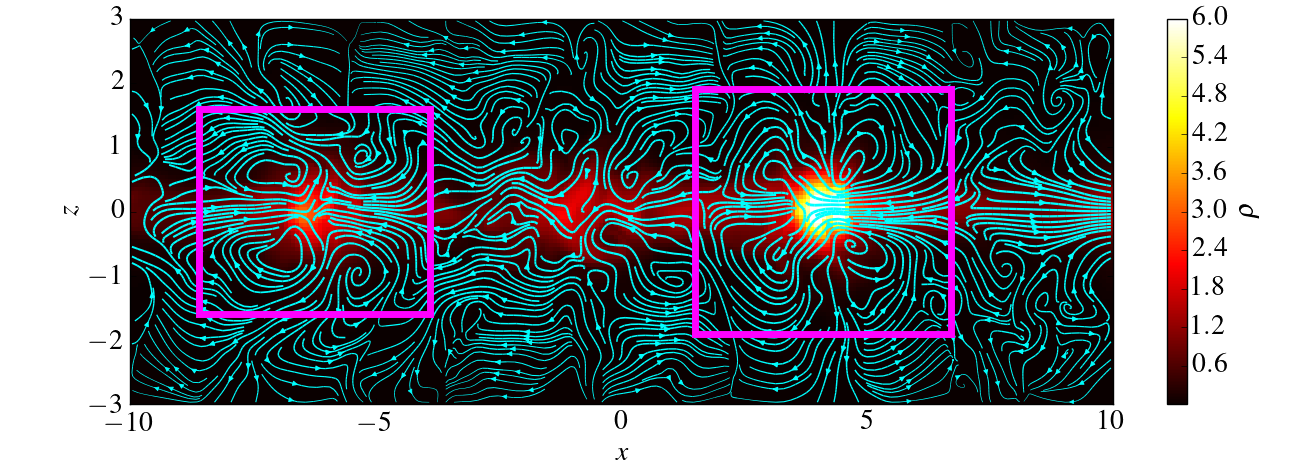
Figure 14: Top: density and streamlines of the GI flow in the poloidal plane ($x,z$) for $\tau_{c}=20\,\Omega^{-1}$ and $\text{Rm}=20$ at a random time of the simulation during the kinematic phase. The thickness of the cyan lines account for the intensity of the poloidal mass flux. The pink rectangles are centred around the density maxima of two prominent spiral GI waves.

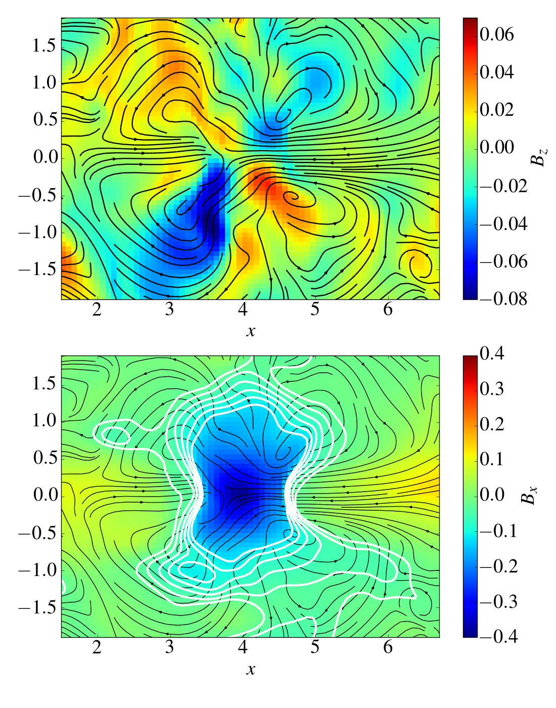
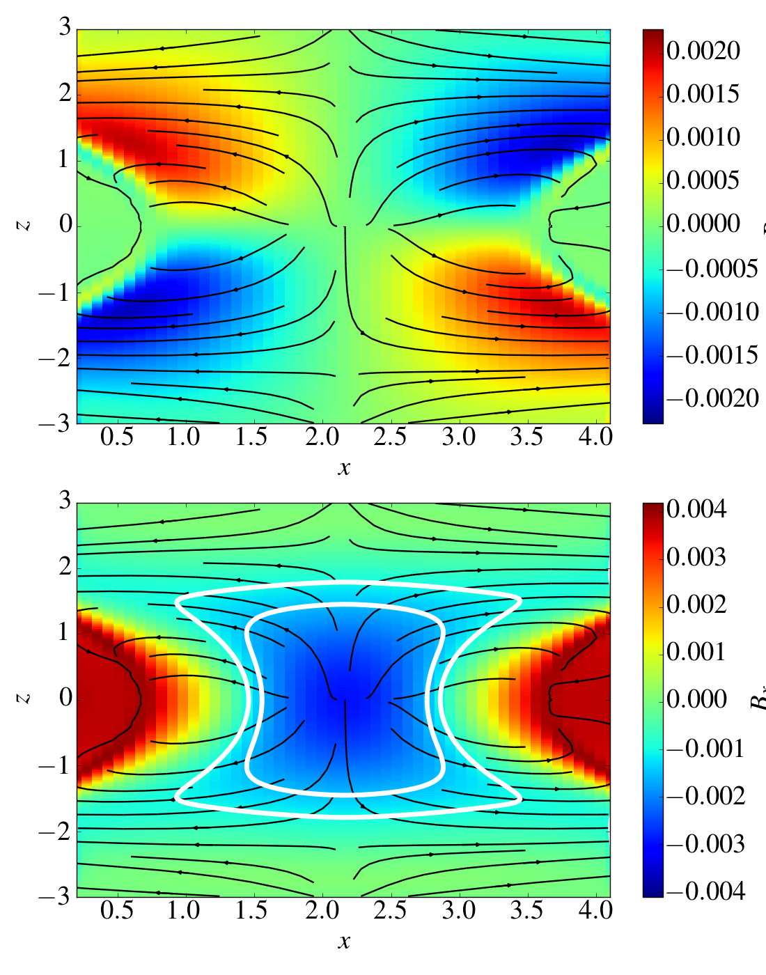
Figure 15: Magnetic field components $B_{z}$ (top) and $B_{x}$ (bottom) projected into the poloidal plane. The black lines are the poloidal streamlines and the white thick lines in the bottom panels are the contours of $B_{x}$ (showing the "mushroom" structure due to radial stretching). The left panels are zoomed around the second spiral wave of Fig. 14 while the right panels are derived from a simulation of a simple spiral wave in polytropic atmosphere. In both cases, the magnetic configuration is invariant along the wave front.

5.2.3 Spiral EMFs and generation of mean $B_{x}$

To further develop the discussion in Section 4.4 and Fig. 9, we examine in detail the connection between the velocities and the EMF profiles. First, the bottom panels of Fig. 13 show the derivative of the EMF $-\mathcal{E}_{y}$ in $z$, projected onto the midplane. For $\text{Rm}=20$, this quantity is concentrated within the density spiral waves and has a positive feedback on the radial field. Averaged over the box, this leads to a mean $\overline{B}_{x}>0$, consistent with Fig. 6. In Section 4.4, we demonstrated that such an EMF is dominated by the $-\tilde{u}_{z}\tilde{b}_{x}$ component near the midplane. Fig. 15 shows that at the location of the density maxima, where $\tilde{b}_{x}<0$, the vertical velocity of the rolls is always directed outward (positive $\tilde{u}_{z}$ if $z>0$ and negative if $z<0$). In the inter-arm regions, this turns to be the opposite configuration. In summary, there is a clear correlation between $u_{z}$ and $b_{x}$ which directly generates a positive gradient of $-\mathcal{E}_{y}$. and then a positive $\overline{B}_{x}$ near the midplane region ($z<0.5H$). Physically, this can be interpreted as a vertical redistribution of radial magnetic flux. The rolls expel the negative flux associated with the spiral outward, but compress the positive flux present in the inter-arm regions. This redistribution happening globally around each spiral wave, favours the configuration depicted in Fig. 6, with a segregation between the midplane region (that builds up $\overline{B}_{x}>0$) and the rest of the disc (that builds up $\overline{B}_{x}<0$).

This vertical redistribution is however incomplete, as we showed that at higher altitudes, most of the radial field is produced through horizontal motions, via the term $\tilde{u}_{x}\tilde{b}_{z}$ (see Section 4.4). Again there is strong evidence that the rolls are involved in this process. In fact, the maximum of $\tilde{u}_{x}\tilde{b}_{z}$ (Fig. 9), located at $z\simeq H$ corresponds exactly to where the radial velocity associated with the rolls is maximum (this also corresponds roughly to their vertical extent). Moreover, Fig. 15 shows that for $z>0.2-0.3H$, the $\tilde{b}_{z}$ component is correlated with the rolls’ horizontal motions. In regions where $u_{x}$ is negative, the magnetic field points outward, and vice-versa. Such correlations lead to a negative EMF $-\mathcal{E}_{y}=\tilde{u}_{x}\,\tilde{b}_{z}$ at $z>0$, resulting in a negative gradient for the EMF and therefore a negative $\overline{B}_{x}$, as expected from Fig. 6 and 9.

5.3 Emergence of small-scale braided structures in the large Rm regime

We showed in Sections 3 and 4.1 that the mean field (or large-scale) dynamo is severely curtailed when Rm increases. Instead, small-scale structures seem to emerge within the spiral waves while the mean field is diminished. We now explore how the flow develops the small-scale magnetic structures and why the mean-field dynamo is optimal at large resistivity.

A quick look at the lower panels of Fig. 13 show that the toroidal EMF for $\text{Rm}=500$ is still contained within the spiral wave but its coherence on longer scales is lost. Parasitic small-scale modes interact with the large-scale magnetic structures depicted in Fig. 15 and subsequently reduce the efficiency of the mean field dynamo.

We show in Fig. 16 (bottom) a 3D rendering of the field line topology around a given spiral wave, chosen randomly in our GI turbulent simulation with $\text{Rm}=500$. To aid interpretation, we show in the top panel the original snapshot containing the full domain with a 2D projection of the field. There is clear a evidence that field lines are rolled and highly twisted within the spiral wave, forming a braided magnetic structure along the wave front. Note that a single structure is formed and settles at the intersection of the four counter-rotating rolls, near the density maximum. The twisting probably results from the combined effect of the differential rotation and the helical flow associated with the spiral rolls. Such complex and intricate structures do not appear in resistive runs, probably because they relax rapidly through diffusion.

Twisted magnetic fields are known to be important in in the context of solar flares and coronal heating, because they are subject to kink instabilities when the twist exceeds a critical value (Dungey & Loughhead, 1954; Roberts, 1956; Hood & Priest, 1981; Bennett et al., 1999). The kink instability mainly deforms and breaks magnetic tubes, and thus efficiently produces turbulent fields and ultimately magnetic energy dissipation. If we define $p$ to be the pitch of the twisted tube and $R_{t}$ its radius, the criterion for instability is

$$pR_{t}=\dfrac{|\nabla\times\mathbf{B}|}{|\mathbf{B}|}R_{t}\gtrsim 1,$$ (20)

(Linton et al., 1996). In our simulations this condition is marginally satisfied, which itself revealing. Though this instability criterion has been derived with simple assumptions and well-defined equilibria (which probably do not apply to GI flows), we believe that braided magnetic fields fields within spiral waves are important in the the generation of small-scale field and the breakdown of the mean field dynamo at larger Rm. Stronger resistivity prevents magnetic field from being twisted into a large number of loops and therefore keeps magnetic energy from cascading to small scales.

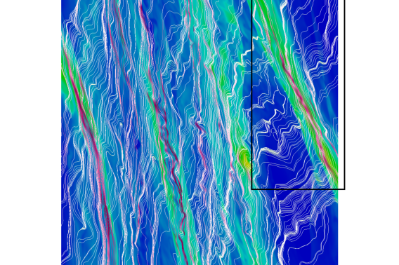
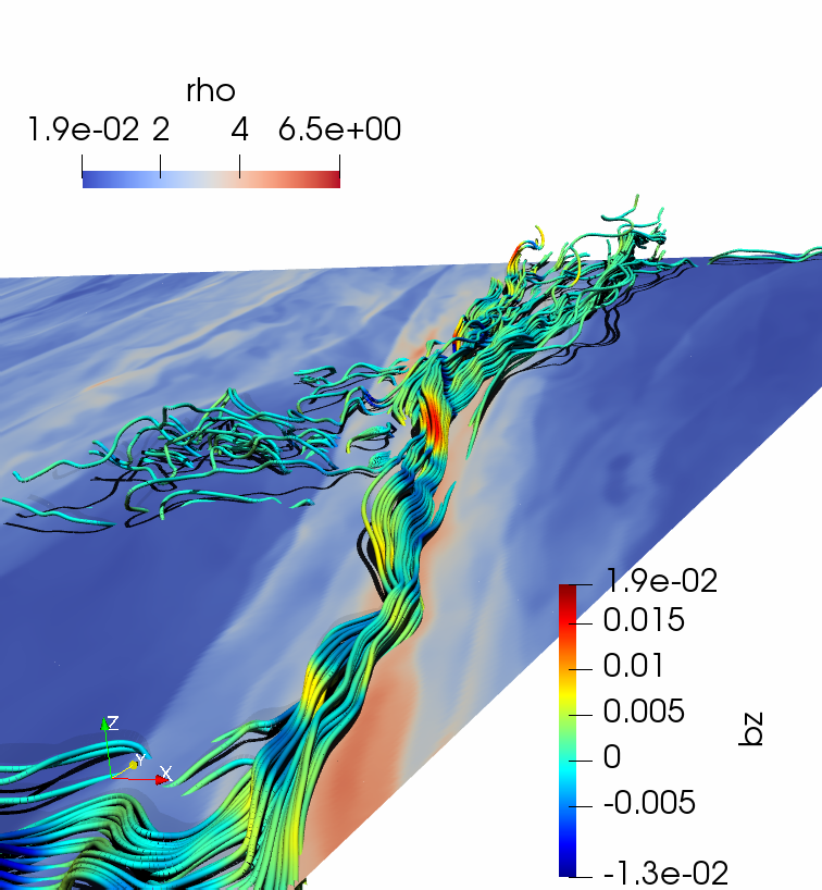
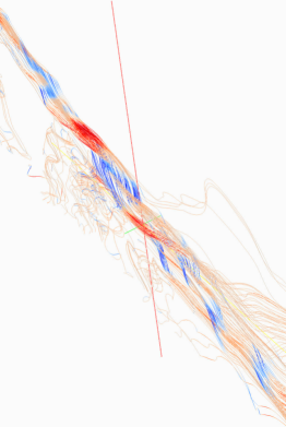
Figure 16: Top: magnetic field lines in the midplane for $\tau_{c}=20\,\Omega^{-1}$ and $\text{Rm}=500$. The blue/green colours represents the gas density (green patterns are spiral waves). The white/pink lines are the magnetic field lines projected into the midplane. Pink color corresponds to high magnetic amplitude, white to low amplitude. The magnetic structure around the most prominent spiral wave (within the black rectangle) is shown in 3D in the lower panels from different angles. The colour of the field lines denotes the amplitude of the vertical field $B_{z}$. The colours in the plane of the left panel indicate the midplane density.

6 Discussion

6.1 Large-scale dynamo

We showed that large-scale fields result from an “alpha" effect which involves vertical folding and horizontal stretching by the rolls associated with spiral waves. The connection between the alpha effect and helicity has often been pointed out, and indeed it can be shown that the spiral rolls are helical, since the wave generates prograde motions where the roll is anti-clockwise and retrograde motions where it is clockwise. As mentioned earlier, the helical motion bears strong similarities with the Roberts flow (Roberts, 1972). But the dynamo loop described above differs significantly from dynamos supported by small-scale subsonic turbulent flow, such as convection in the Sun. The motions here are supersonic, large scale and highly localized in radius, which leads to a rather patchy and inhomogeneous $B_{y}$, different from the initial uniform $B_{y}$. Fields are inevitably filamentary and sparse in such GI flows. Finally, we point out that 20% of the mean field might also come from small-scale turbulence, or inertial and helical waves triggered by a parametric instability.

6.2 Boundary conditions

One concern is that the dynamo behaviour differs when using different boundary conditions (see Section 3.4). In particular, the strong and large-scale dynamo at low Rm is conditioned by the existence of a net toroidal field throughout the box. However we think that this issue is not critical for several reasons.

First, and perhaps most obviously, the dynamo still works with periodic boundaries. This suggests that magnetic field amplification mechanism is not an artefact of the boundary. In particular, the growth rates obtained with open boundaries increase with decreasing $\tau_{c}$, which is physically expected. The EMF at the boundaries in that case is relatively small compared to the EMF near the midplane (see Fig. 8). In a periodic box, we also checked that a large-scale field $\overline{\mathbf{B}}(z)$ can be generated, although it exhibits a weaker amplitude and flips regularly, every 5 or 6 orbits. Perhaps, one key question is to understand whether the dynamo in this configuration is supported by the large-scale $\overline{\mathbf{B}}(z)$ or by a small-scale process of Zeld’ovich type. The answer is not obvious, since the Rm regime allowing the dynamo is marginally resolved by our simulations. In any cases, the stretching and folding by the spiral rolls must be crucial in the dynamo mechanism, whatever kind it is.

Second, boundary conditions are part of the physical problem, and open boundaries are the most realistic of the options available to us. Periodic boundary conditions introduce unnatural communication between the two surfaces of the discs which can alter the nature of the large-scale field, as we see. Moreover, periodic boundaries do not allow magnetic buoyancy to evacuate excess magnetic field; its continued build-up may be unphysical. They also force a particular geometry upon the field, which can artificially enhance its dissipation. In real systems, the disc exchanges field with an external “corona”, though the details of how this works is not easily determined.

6.3 Application to protoplanetary discs

The dynamo identified in this work is perhaps most relevant for young and massive protoplanetary discs, subject to GI. Indeed, except for the innermost regions ($\lesssim$ 1 AU), the coupling between the gas and magnetic field in these object is believed to be weak, and non-ideal MHD effects should be important throughout, and certainly in the regions susceptible to gravitational instability (typically beyond 20 AU). According to Simon et al. (2015), using the standard MMSN disc model, the magnetic Reynolds number in these regions varies between $10^{3}$ and $10^{6}$. However these numbers must be considered gross upper limits for the denser and flatter discs susceptible to GI (see the case Elias 2-27 for instance, Pérez et al., 2016). The reason is that FUV cannot penetrate very far into the disc when the surface density is high. We expect then that some of the Rm probed by our simulations are relevant.

In any case, ohmic diffusion is not the most dominant non-ideal effect at radii larger than 20 AU. Ambipolar diffusion is believed to be the leading effect in these regions with typical Reynolds (or Elsasser) numbers between 1 and 1000 (Simon et al., 2015). Although our numerical set-up does not capture ambipolar diffusion, it is not excluded that its effect may be similar to ohmic diffusion in the nonlinear phase of the dynamo, at least if the magnetic field is not highly anisotropic. We point out again that during the dynamo’s kinematic phase, both the Hall effect and ambipolar diffusion are subdominant to ohmic resistivity, though this may change if there is a net magnetic field. Future simulations are necessary to address how ambipolar diffusion and the Hall effect influence the GI dynamo process, but also more generally on GI turbulence. For example, it is possible that zonal flows enhanced by non-ideal effects (Lesur et al., 2014; Bai, 2015) significantly perturb the spiral waves motions or become even unstable to non-axisymmetric perturbations (Vanon & Ogilvie, 2016), leading to different flow behaviour.

It has been postulated that somewhat older disks may periodically undergo GI in their magnetically inactive dead-zones (located between roughly 1 and 10 AU) during outbursts of FU Ori or EX Lupi type (Gammie, 1996; Armitage et al., 2001; Zhu et al., 2010). In affected regions the magnetic Reynolds number is low, and a GI dynamo is a distinct possibility in the initial stages of an outburst, perhaps supplying the seed field for the onset of MRI. The interplay of the GI, GI dynamo, the MRI, and the Hall effect are expected to present some intriguing dynamics.

We finally give estimates of the field intensity in PP discs that a GI-dynamo might be able to generate. In the range of Reynolds number probed by our simulations, we found that the ratio of magnetic to thermal pressure $P$ lies in a range between 0.01 and 0.5 (depending on Rm). We have $P=\rho c_{s}^{2}/\gamma\simeq\Sigma H\Omega^{2}/(\sqrt{2\pi})$. We consider a typical disc with surface density

$$\Sigma\simeq 810\,\left(\frac{R}{\text{1 AU}}\right)^{-0.8}$ g/cm$^{2}$$ (21)

and $H/R\simeq 0.04$ in agreement with observations of Elias 2-27 (Cieza et al., 2017), a massive disc susceptible to GI. By considering a disc with a central star mass equal to that of the Sun, we then hobtain

$$B\simeq 0.4-2.5\left(\frac{R}{\text{1 AU}}\right)^{-1.4}\text{Gauss}$$ (22)

At $R=30$ AU we estimate the field strength to be around $B\simeq 3\,-20\,m\text{G}$. We remind the reader that such fields are mainly toroidal, if generated through GI spiral waves.

6.4 Application to AGN

The GI dynamo could be also excited in the regions of AGN beyond 0.01 pc, where self-gravity is thought to dominate (Menou & Quataert, 2001; Goodman, 2003; Lodato, 2007). The typical Rm in these objects at these radii is poorly constrained: though the disk is very large, the ionisation fraction could dip to low levels as the gas is too cool to support significant thermal ionisation. One must then appeal to photoionisation, the efficiency of which is uncertain at the midplane, and partly controlled by the morphology of the disk. It is likely, however, that typical Rm values are greater than those probed here. The same claims can be made with respect to the ambipolar Reynolds number (Menou & Quataert, 2001). Thus making a direct comparison with AGN is not straightforward.

The saturated magnetic energy of the dynamo never exceeds the thermal energy (cf. Fig. 4), but can nonetheless reach significant levels, with $\beta_{t}\sim 2$. Concurrently, the saturated Toomre Q does attain somewhat larger values (Fig. 5). We might then conclude that a saturated GI dynamo, when up and running, could help prevent a disk from fragmenting when it might otherwise. The thin AGN disk would then extend to larger radii than current hydrodynamical estimates predict, though it is unlikely that the dynamo’s magnetic pressure on it own can completely solve the disk truncation problem (see Goodman, 2003). Adding a vertical magnetic field of sufficient strength may be one possible solution here (RL18a). (Note that a completely analogous discussion can be had regarding giant planet formation in PP disks.) In any case, it is certainly likely that the GI and its interaction with magnetic fields are foremost elements in the mysterious dynamics of the broad line regions of AGN.

6.5 Applications to galaxies

Multiwavelength radio observations suggest that some spiral galaxies (M81, M51 and possibly M33) are dominated by bisymmetric-spiral magnetic fields. These magnetic spiral patterns are strongly correlated with the large scale galactic spiral arms.

To explain the correlation, Chiba & Tosa (1990) and Hanasz et al. (1991) proposed a parametric swing excitation due to resonances between weak magnetic wave oscillations and density spiral waves. More sophisticated models of this resonance have been studied (Moss, 1997; Rohde et al., 1999), but most are based on a mean-field theory, in which the interstellar turbulence, driven by supernovae, is parametrized by an alpha effect (Elstner et al., 2000; Rüdiger & Hollerbach, 2004; Gressel et al., 2008). On the whole, the mean field theory provides an acceptable match to the observations, though is not without its challenges (see, for example Nixon et al., 2018; Tabatabaei et al., 2016). Alternative theories, based on the vertical shear of a primordial poloidal field, have been also proposed but remain highly speculative (Nixon et al., 2018). Surprisingly, density spiral waves have rarely been considered as capable of amplifying magnetic fields on their own. Instead density waves have been historically treated as a process that could shape large-scale fields already generated. Only recent MHD simulations of galactic discs have suggested some link between the dynamo and the spiral arms (Dobbs et al., 2016; Khoperskov & Khrapov, 2018). Our GI-simulations show that such waves can, in principle, act as a dynamo and produce spiral magnetic patterns, similar to those observed in galaxies.

Although there is a consensus that GI is active in galaxies, there is however some uncertainty regarding the magnetic diffusivity. The microscopic or Spitzer resistivity in galactic disc is about $10^{8}$ cm²/s (Parker, 1972), which yields gigantic magnetic Reynolds numbers. On the other hand, we could invoke an anomalous resistivity due to small-scale turbulence in order to explain dissipation of small scale fluctuations in the ISM (Hanasz et al., 2009). The common value used is $\eta=10^{26}$ cm²/s (300 pc² Myr^-1), which presents magnetic Reynolds number between 10 and $10^{4}$. This indeed overlaps the range of Rm explored by our simulations.

Assuming a surface density of $0.02$ g/cm^-2 for $R\lesssim 10$ kpc, a typical scaleheight of 1000 parsecs, and a rotation period of 200 Myrs, we find that the GI-dynamo produces $B\simeq 2\,\mu\text{G}-5\,\mu\text{G}$ for $\text{Rm}\sim 10-100$ in a handful of orbits. On the other hand, radio-faint galaxies like M31 and M33 possess fields strength of about 5 $\mu\text{G}$, while gas-rich galaxies with high star-formation rates, like M51, M83 and NGC 6946 possess $15\mu\text{G}$ on average. We stress, however, that direct comparison is difficult and relies on various, somewhat dubious, assumptions. The value of the anomalous resistivity found in the literature is ad-hoc and estimated from simulations or mean field models. Moreover, our simulations do not describe the rich assortment of physical processes occurring in galactic disc gas, such as supernova driven-turbulence or other stellar feedback. Simulations taking into account these effects are necessary to assess their relative importance in comparison to GI. Other than differences in thermodynamics, one of the more glaring discrepancies is our use of a Keplerian rotation law which is, of course, inappropriate for galaxies, though easily rectified in future simulations. Finally, our local model cannot describe the development of the bar instability, which itself may impact significantly (positively or negatively) on a galaxy’s magnetic field generation.

7 Conclusions

In summary, we performed 3D MHD stratified shearing box simulations, with zero-net magnetic flux, in order to assess the ability of gravito-turbulence to sustain a dynamo in the presence of finite and uniform resistivity. In Section 3 and 4, we explored the fundamental properties of the dynamo by probing a wide range of magnetic Reynolds numbers, cooling times, and boundary conditions. We obtained the following results:

1. The dynamo works for cooling times between $\tau_{c}=5$ (which corresponds roughly to the fragmentation threshold) and $100\,\Omega^{-1}$. Growth rates and saturated magnetic energy decrease with $\tau_{c}$.
   

2. The dynamo is robust to boundary conditions, but its properties depends on which boundary condition is applied vertically (periodic or open).
   

3. In the case of open boundaries, the critical magnetic Reynolds number is of order unity ($\text{Rm}_{c}\simeq 4$ for $\tau_{c}=\,20\Omega^{-1}$). It is around 200 when periodic boundary conditions are used.
   

4. Magnetic energy reaches quasi-equipartition with kinetic pressure ($\beta_{t}=1$) for $\text{Rm}\lesssim 100$. For larger Rm however, the dynamo growth rate and saturated magnetic energy drop with Rm, which suggests that the dynamo is “slow". However this last statement has to be taken with caution since it is not possible to predict the dynamo behavior in the large magnetic Reynolds number limit.
   

5. The dynamo is essentially large scale, kinematic and of mean field type, although smaller magnetic scales emerge at large Rm. It is powered by both differential rotation and large-scale spiral waves motion.

In Section 5, we investigated the role of spiral waves in the magnetic field amplification and proposed a model inspired by the solar dynamo cycle and based on the classical $\alpha$-$\Omega$ theory of Parker (1955). This model assumes that:

1. Horizontal motions associated with spiral waves compress an initial toroidal field along the density waves.

2. Pairs of vertical counter-rotating rolls (associated with the density wave) pinch the field, lift, and fold it, generating new radial field.

3. The disk’s differential rotation shears out the radial field to regenerate toroidal field, and the loop is closed.

We demonstrated that the vertical EMF profiles giving rise to the large-scale field are generated by the rolls. At large Rm, we found however that the large-scale magnetic ropes inside the spiral waves are braided and broken by small-scale parasitic modes, probably associated with a kink instability. Small-scale fast reconnection processes, like the tearing instability, might also be involved in the destruction of the large scale field at large Rm.

As discussed in Section 6, the GI-dynamo could have direct application to young and massive gravito-turbulent stellar discs, since these objects are cold and exhibit large resistivities. In the coming years, ALMA will have the potential to directly infer magnetic field orientation by measuring Zeeman splitting of cyanide lines. This technique has been already utilised to explore large-scale massive objects such as molecular clouds, but is now applicable to circumstellar discs (Brauer et al., 2017). This raises the hope of detecting spiral magnetic patterns in PP discs and therefore of characterizing their dynamo behaviour. The highly resistive dead zones of older PP disks undergoing outbursts are another venue in which the GI dynamo phenomena might appear, possibly seeding the field necessary to “kickstart” the MRI. More speculatively, our work might be applied to galactic dynamos, which so far have only been addressed within the framework of mean field theory. Our main result is that spiral waves can directly produce dynamo action in these objects as well as the observed alignment between magnetic and density spiral patterns This result is in particular reminiscent of galactic dynamo simulations by Khoperskov & Khrapov (2018). So too, might the dynamo work in the cooler outer radii of AGN disks.

Finally, we emphasise that characterising the behaviour of the dynamo at Rm larger than a thousand is not yet possible with our simulations, because of resolution issues. This potentially limits application of the theory to more astrophysical settings. In addition, future work will be necessary to better understand the effect not only of low resistivity but also other non-ideal effects, ambipolar diffusion especially. Discs are also generally threaded by a net vertical field; the impact of such large scale component remains unclear and will be treated separately.

References

- Armitage (2015) Armitage P. J., 2015, preprint, (arXiv:1509.06382)
- Armitage et al. (2001) Armitage P. J., Livio M., Pringle J. E., 2001, MNRAS, 324, 705
- Bai (2013) Bai X.-N., 2013, ApJ, 772, 96
- Bai (2015) Bai X.-N., 2015, ApJ, 798, 84
- Balbus (2003) Balbus S. A., 2003, ARA&A, 41, 555
- Balbus & Hawley (1991) Balbus S. A., Hawley J. F., 1991, ApJ, 376, 214
- Balbus & Henri (2008) Balbus S. A., Henri P., 2008, ApJ, 674, 408
- Bennett et al. (1999) Bennett K., Roberts B., Narain U., 1999, Solar physics, 185, 41
- Boley & Durisen (2006) Boley A. C., Durisen R. H., 2006, ApJ, 641, 534
- Brandenburg (2018) Brandenburg A., 2018, preprint, (arXiv:1801.05384)
- Brandenburg & Subramanian (2005) Brandenburg A., Subramanian K., 2005, Phys. Rep., 417, 1
- Brandenburg et al. (1995) Brandenburg A., Nordlund A., Stein R. F., Torkelsson U., 1995, ApJ, 446, 741
- Brauer et al. (2017) Brauer R., Wolf S., Flock M., 2017, AAp, 607, A104
- Carrasco-González et al. (2010) Carrasco-González C., Rodríguez L. F., Anglada G., Martí J., Torrelles J. M., Osorio M., 2010, Science, 330, 1209
- Chiba & Tosa (1990) Chiba M., Tosa M., 1990, MNRAS, 244, 714
- Choudhuri (1984) Choudhuri A. R., 1984, ApJ, 281, 846
- Christiaens et al. (2014) Christiaens V., Casassus S., Perez S., van der Plas G., Ménard F., 2014, ApJl, 785, L12
- Cieza et al. (2017) Cieza L. A., et al., 2017, ApJl, 851, L23
- Dobbs et al. (2016) Dobbs C. L., Price D. J., Pettitt A. R., Bate M. R., Tricco T. S., 2016, MNRAS, 461, 4482
- Donati et al. (2005) Donati J.-F., Paletou F., Bouvier J., Ferreira J., 2005, Nature, 438, 466
- Dong et al. (2016) Dong R., Vorobyov E., Pavlyuchenkov Y., Chiang E., Liu H. B., 2016, ApJ, 823, 141
- Dungey & Loughhead (1954) Dungey J. W., Loughhead R. E., 1954, Australian Journal of Physics, 7, 5
- Durisen et al. (2007) Durisen R. H., Boss A. P., Mayer L., Nelson A. F., Quinn T., Rice W. K. M., 2007, Protostars and Planets V, pp 607–622
- Elstner et al. (2000) Elstner D., Otmianowska-Mazur K., von Linden S., Urbanik M., 2000, AAp, 357, 129
- Federrath et al. (2011) Federrath C., Sur S., Schleicher D. R. G., Banerjee R., Klessen R. S., 2011, ApJ, 731, 62
- Fleming et al. (2000) Fleming T. P., Stone J. M., Hawley J. F., 2000, ApJ, 530, 464
- Fletcher et al. (2011) Fletcher A., Beck R., Shukurov A., Berkhuijsen E. M., Horellou C., 2011, MNRAS, 412, 2396
- Fromang et al. (2007) Fromang S., Papaloizou J., Lesur G., Heinemann T., 2007, A&A, 476, 1123
- Gammie (1996) Gammie C. F., 1996, ApJ, 457, 355
- Gammie (2001) Gammie C. F., 2001, ApJ, 553, 174
- Goddi et al. (2017) Goddi C., Surcis G., Moscadelli L., Imai H., Vlemmings W. H. T., van Langevelde H. J., Sanna A., 2017, AAp, 597, A43
- Goldreich & Lynden-Bell (1965) Goldreich P., Lynden-Bell D., 1965, MNRAS, 130, 125
- Goodman (2003) Goodman J., 2003, MNRAS, 339, 937
- Gressel (2010) Gressel O., 2010, MNRAS, 405, 41
- Gressel et al. (2008) Gressel O., Elstner D., Ziegler U., Rüdiger G., 2008, AAp, 486, L35
- Guilet & Ogilvie (2013) Guilet J., Ogilvie G. I., 2013, MNRAS, 430, 822
- Hanasz et al. (1991) Hanasz M., Lesch H., Krause M., 1991, AAp, 243, 381
- Hanasz et al. (2009) Hanasz M., Otmianowska-Mazur K., Kowal G., Lesch H., 2009, AAp, 498, 335
- Hawley et al. (1995) Hawley J. F., Gammie C. F., Balbus S. A., 1995, ApJ, 440, 742
- Hirose & Shi (2017) Hirose S., Shi J.-M., 2017, MNRAS, 469, 561
- Hood & Priest (1981) Hood A. W., Priest E. R., 1981, Geophysical and Astrophysical Fluid Dynamics, 17, 297
- Jouve et al. (2008) Jouve L., et al., 2008, AAp, 483, 949
- Käpylä & Korpi (2011) Käpylä P. J., Korpi M. J., 2011, MNRAS, 413, 901
- Käpylä et al. (2010) Käpylä P. J., Korpi M. J., Brandenburg A., 2010, AAp, 518, A22
- Khoperskov & Khrapov (2018) Khoperskov S. A., Khrapov S. S., 2018, AAp, 609, A104
- Kim & Ostriker (2001) Kim W.-T., Ostriker E. C., 2001, ApJ, 559, 70
- Kratter & Lodato (2016) Kratter K. M., Lodato G., 2016, preprint, (arXiv:1603.01280)
- Krause & Raedler (1980) Krause F., Raedler K.-H., 1980, Mean-field magnetohydrodynamics and dynamo theory
- Kunz & Balbus (2004) Kunz M. W., Balbus S. A., 2004, MNRAS, 348, 355
- Latter & Papaloizou (2017) Latter H. N., Papaloizou J., 2017, MNRAS, 472, 1432
- Lesur et al. (2014) Lesur G., Kunz M. W., Fromang S., 2014, AAp, 566, A56
- Linton et al. (1996) Linton M. G., Longcope D. W., Fisher G. H., 1996, ApJ, 469, 954
- Liu et al. (2016) Liu H. B., et al., 2016, Science Advances, 2, e1500875
- Lodato (2007) Lodato G., 2007, Nuovo Cimento Rivista Serie, 30
- Mann et al. (2015) Mann R. K., Andrews S. M., Eisner J. A., Williams J. P., Meyer M. R., Di Francesco J., Carpenter J. M., Johnstone D., 2015, ApJ, 802, 77
- Meheut et al. (2015) Meheut H., Fromang S., Lesur G., Joos M., Longaretti P.-Y., 2015, AAp, 579, A117
- Menou & Quataert (2001) Menou K., Quataert E., 2001, ApJ, 552, 204
- Mignone et al. (2007) Mignone A., Bodo G., Massaglia S., Matsakos T., Tesileanu O., Zanni C., Ferrari A., 2007, ApJs, 170, 228
- Moffatt (1977) Moffatt H. K., 1977, Magnetic field generation in electrically conducting fluids.. Cambridge University Press
- Moss (1997) Moss D., 1997, MNRAS, 289, 554
- Nixon et al. (2018) Nixon C. J., Hands T. O., King A. R., Pringle J. E., 2018, MNRAS, 477, 3539
- Ogilvie & Lubow (2002) Ogilvie G. I., Lubow S. H., 2002, MNRAS, 330, 950
- Oishi & Mac Low (2011) Oishi J. S., Mac Low M.-M., 2011, ApJ, 740, 18
- Paardekooper (2012) Paardekooper S.-J., 2012, MNRAS, 421, 3286
- Parker (1955) Parker E. N., 1955, ApJ, 122, 293
- Parker (1972) Parker E. N., 1972, ApJ, 174, 499
- Parker (1979) Parker E. N., 1979, Cosmical magnetic fields: Their origin and their activity
- Pérez et al. (2016) Pérez L. M., et al., 2016, Science, 353, 1519
- Pudritz (1981) Pudritz R. E., 1981, MNRAS, 195, 881
- Pudritz & Silk (1989) Pudritz R. E., Silk J., 1989, ApJ, 342, 650
- Rice et al. (2003) Rice W. K. M., Armitage P. J., Bate M. R., Bonnell I. A., 2003, MNRAS, 339, 1025
- Riols & Latter (2016) Riols A., Latter H., 2016, MNRAS, 460, 2223
- Riols & Latter (2018a) Riols A., Latter H., 2018a, MNRAS, 474, 2212
- Riols & Latter (2018b) Riols A., Latter H., 2018b, MNRAS, 476, 5115
- Riols et al. (2017a) Riols A., Latter H., Paardekooper S.-J., 2017a, MNRAS, 471, 317
- Riols et al. (2017b) Riols A., Rincon F., Cossu C., Lesur G., Ogilvie G. I., Longaretti P.-Y., 2017b, AA, 598, A87
- Roberts (1956) Roberts P. H., 1956, ApJ, 124, 430
- Roberts (1972) Roberts G. O., 1972, Philosophical Transactions of the Royal Society of London Series A, 271, 411
- Rohde et al. (1999) Rohde R., Rüdiger G., Elstner D., 1999, AAp, 347, 860
- Rüdiger & Hollerbach (2004) Rüdiger G., Hollerbach R., 2004, The magnetic universe : geophysical and astrophysical dynamo theory
- Sano et al. (2000) Sano T., Miyama S. M., Umebayashi T., Nakano T., 2000, ApJ, 543, 486
- Shi & Chiang (2014) Shi J.-M., Chiang E., 2014, ApJ, 789, 34
- Simon et al. (2012) Simon J. B., Beckwith K., Armitage P. J., 2012, MNRAS, 422, 2685
- Simon et al. (2015) Simon J. B., Lesur G., Kunz M. W., Armitage P. J., 2015, MNRAS, 454, 1117
- Stephens et al. (2014) Stephens I. W., et al., 2014, Nature, 514, 597
- Tabatabaei et al. (2016) Tabatabaei F. S., Martinsson T. P. K., Knapen J. H., Beckman J. E., Koribalski B., Elmegreen B. G., 2016, ApJ, 818, L10
- Tobin et al. (2013) Tobin J. J., et al., 2013, ApJ, 779, 93
- Toomre (1964) Toomre A., 1964, ApJ, 139, 1217
- Vanon & Ogilvie (2016) Vanon R., Ogilvie G. I., 2016, MNRAS, 463, 3725
- Wang & Silk (1994) Wang B., Silk J., 1994, ApJ, 427, 759
- Wardle (1999) Wardle M., 1999, MNRAS, 307, 849
- Wardle (2007) Wardle M., 2007, APSS, 311, 35
- Wardle & Salmeron (2012) Wardle M., Salmeron R., 2012, MNRAS, 422, 2737
- Zhu & Stone (2018) Zhu Z., Stone J. M., 2018, ApJ, 857, 34
- Zhu et al. (2010) Zhu Z., Hartmann L., Gammie C., 2010, ApJ, 713, 1143