Concise Explanations of Neural Networks using Adversarial Training

Prasad Chalasani    Jiefeng Chen    Amrita Roy Chowdhury    Somesh Jha    Xi Wu
Abstract

We show new connections between adversarial learning and explainability for deep neural networks (DNNs). One form of explanation of the output of a neural network model in terms of its input features, is a vector of feature-attributions. Two desirable characteristics of an attribution-based explanation are: (1) sparseness: the attributions of irrelevant or weakly relevant features should be negligible, thus resulting in concise explanations in terms of the significant features, and (2) stability: it should not vary significantly within a small local neighborhood of the input. Our first contribution is a theoretical exploration of how these two properties (when using attributions based on Integrated Gradients, or IG) are related to adversarial training, for a class of 1-layer networks (which includes logistic regression models for binary and multi-class classification); for these networks we show that (a) adversarial training using an subscript\ell_{\infty}-bounded adversary produces models with sparse attribution vectors, and (b) natural model-training while encouraging stable explanations (via an extra term in the loss function), is equivalent to adversarial training. Our second contribution is an empirical verification of phenomenon (a), which we show, somewhat surprisingly, occurs not only in 1-layer networks, but also DNNs trained on standard image datasets, and extends beyond IG-based attributions, to those based on DeepSHAP: adversarial training with subscript\ell_{\infty}-bounded perturbations yields significantly sparser attribution vectors, with little degradation in performance on natural test data, compared to natural training. Moreover, the sparseness of the attribution vectors is significantly better than that achievable via 1subscript1\ell_{1}-regularized natural training.

Attribution, Explainability, Adversarial, Logistic

1 Introduction

Despite the recent dramatic success of deep learning models in a variety of domains, two serious concerns have surfaced about these models.

Vulnerability to Adversarial Attacks:

We can abstractly think of a neural network model as a function F(𝐱)𝐹𝐱F(\operatorname{{\boldsymbol{x}}}) of a d𝑑d-dimensional input vector 𝐱d𝐱superscript𝑑\operatorname{{\boldsymbol{x}}}\in\mathbb{R}^{d}, and the range of F𝐹F is either a discrete set of class-labels, or a continuous set of class probabilities. Many of these models can be foiled by an adversary who imperceptibly (to humans) alters the input 𝐱𝐱\operatorname{{\boldsymbol{x}}} by adding a perturbation δd𝛿superscript𝑑\delta\in\mathbb{R}^{d} so that F(𝐱+δ)𝐹𝐱𝛿F(\operatorname{{\boldsymbol{x}}}+\delta) is very different from F(𝐱)𝐹𝐱F(\operatorname{{\boldsymbol{x}}}) (Szegedy et al., 2013; Goodfellow et al., 2014; Papernot et al., 2015; Biggio et al., 2013). Adversarial training (or adversarial learning) has recently been proposed as a method for training models that are robust to such attacks, by applying techniques from the area of Robust Optimization (Madry et al., 2017; Sinha et al., 2018). The core idea of adversarial training is simple: we define a set S𝑆S of allowed perturbations δd𝛿superscript𝑑\delta\in\mathbb{R}^{d} that we want to “robustify” against (e.g. S𝑆S could be the set of δ𝛿\delta where δεsubscriptnorm𝛿𝜀||\delta||_{\infty}\leq\varepsilon), and perform model-training using Stochastic Gradient Descent (SGD) exactly as in natural training, except that each training example x𝑥x is perturbed adversarially, i.e. replaced by x+δ𝑥superscript𝛿x+\delta^{*} where δSsuperscript𝛿𝑆\delta^{*}\in S maximizes the example’s loss-contribution.

Explainability:

One way to address the well-known lack of explainability of deep learning models is feature attribution, which aims to explain the output of a model F(𝐱)𝐹𝐱F(\operatorname{{\boldsymbol{x}}}) as an attribution vector AF(𝐱)superscript𝐴𝐹𝐱A^{F}(\operatorname{{\boldsymbol{x}}}) of the contributions from the features 𝐱𝐱\operatorname{{\boldsymbol{x}}}. There are several feature-attribution techniques in the literature, such as Integrated Gradients (IG) (Sundararajan et al., 2017), DeepSHAP (Lundberg & Lee, 2017), and LIME (Ribeiro et al., 2016). For such an explanation to be human-friendly, it is highly desirable (Molnar, 2019) that the attribution-vector is sparse, i.e., only the features that are truly predictive of the output F(𝐱)𝐹𝐱F(\operatorname{{\boldsymbol{x}}}) should have significant contributions, and irrelevant or weakly-relevant features should have negligible contributions. A sparse attribution makes it possible to produce a concise explanation, where only the input features with significant contributions are included. For instance, if the model F𝐹F is used for a loan approval decision, then various stakeholders (like customers, data-scientists and regulators) would like to know the reason for a specific decision in simple terms. In practice however, due to artifacts in the training data or process, the attribution vector is often not sparse and irrelevant or weakly-relevant features end up having significant contributions (Tan et al., 2013). Another desirable property of a good explanation is stability: the attribution vector should not vary significantly within a small local neighborhood of the input x𝑥x. Similar to the lack of concise explainability, natural training often results in explanations that lack stability (Alvarez-Melis & Jaakkola, 2018).

Our paper shows new connections between adversarial robustness and the above-mentioned desirable properties of explanations, namely conciseness and stability. Specifically, let F~~𝐹\tilde{F} be an adversarially trained version of a classifier F𝐹F, and for a given input vector 𝐱𝐱\operatorname{{\boldsymbol{x}}} and attribution method A𝐴A, let AF(𝐱)superscript𝐴𝐹𝐱A^{F}(\operatorname{{\boldsymbol{x}}}) and AF~(𝐱)superscript𝐴~𝐹𝐱A^{\tilde{F}}(\operatorname{{\boldsymbol{x}}}) denote the corresponding attribution vectors. The central research question this paper addresses is:

Is AF~(𝐱)superscript𝐴~𝐹𝐱A^{\tilde{F}}(\operatorname{{\boldsymbol{x}}}) sparser and more stable than AF(𝐱)superscript𝐴𝐹𝐱A^{F}(\operatorname{{\boldsymbol{x}}})?

The main contributions of our paper are as follows:

Theoretical Analysis of Adversarial Training: Our first set of results show via a theoretical analysis that (ε)subscript𝜀\ell_{\infty}(\varepsilon)-adversarial training 1-layer networks tends to produce sparse attribution vectors for IG, which in turn leads to concise explanations. In particular, under some assumptions, we show (Theorems 3.1 and E.1) that for a general class of convex loss functions (which includes popular loss functions used in 1-layer networks, such as logistic and hinge loss, used for binary or multi-class classification), and adversarial perturbations δ𝛿\delta satisfying δεsubscriptnorm𝛿𝜀||\delta||_{\infty}\leq\varepsilon, the weights of “weak” features are on average more aggressively shrunk toward zero than during natural training, and the rate of shrinkage is proportional to the amount by which ε𝜀\varepsilon exceeds a certain measure of the “strength” of the feature. This shows that (ε)subscript𝜀\ell_{\infty}(\varepsilon)-adversarial training tends to produce sparse weight vectors in popular 1-layer models. In Section 4 we show (Lemma 4.1) a closed form formula for the IG vector of 1-layer models, that makes it clear that in these models, sparseness of the weight vector directly implies sparseness of the IG vector.

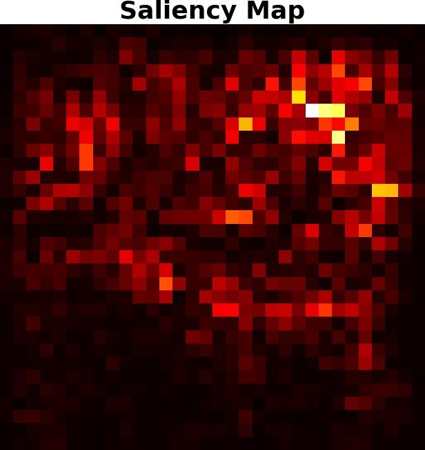
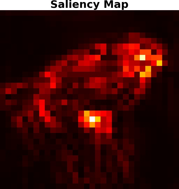
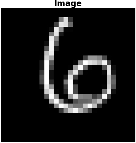
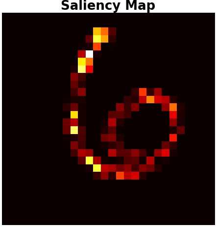
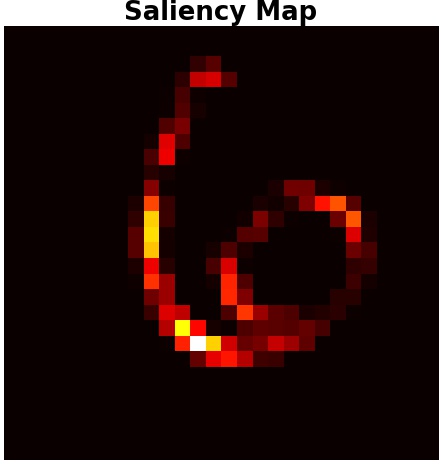
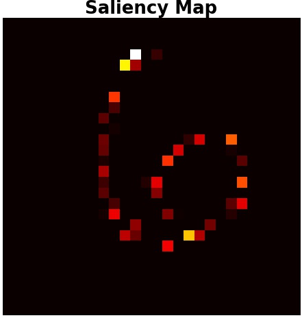
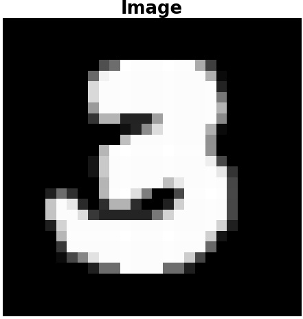
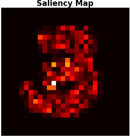
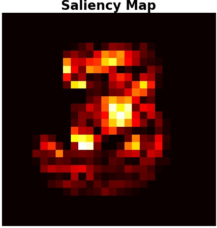
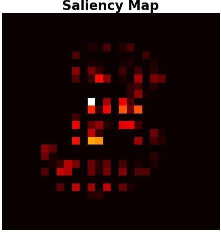
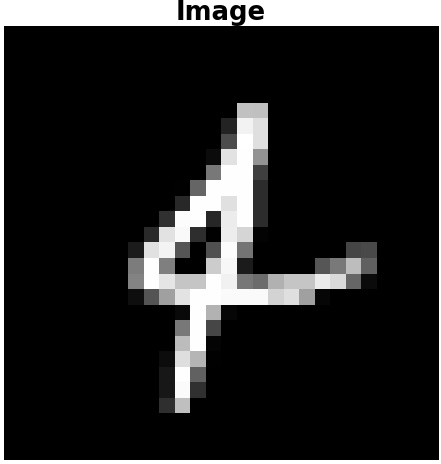
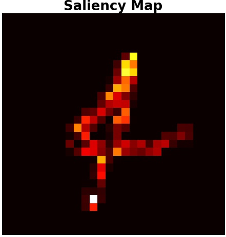
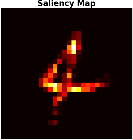
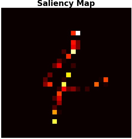
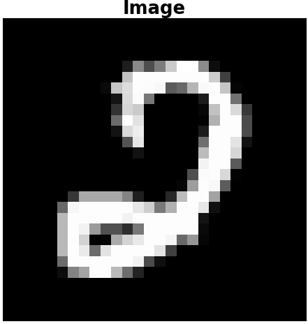
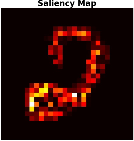
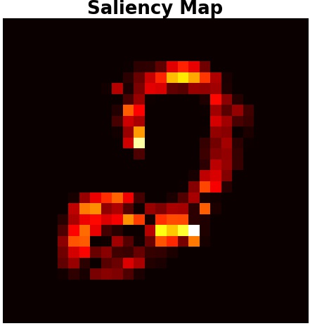
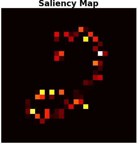
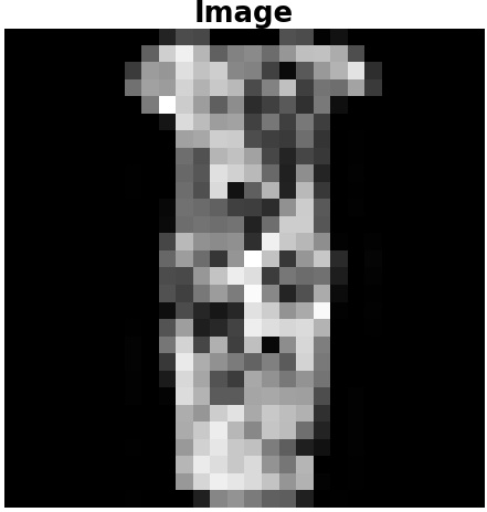
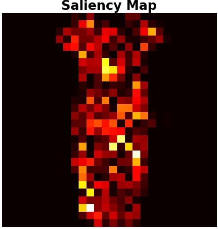
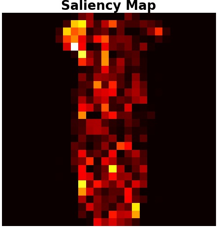
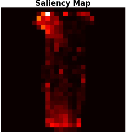
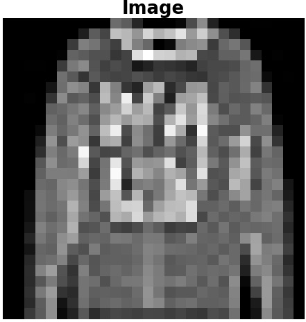
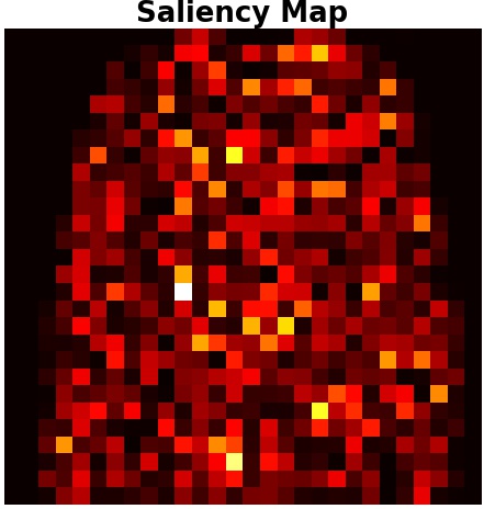
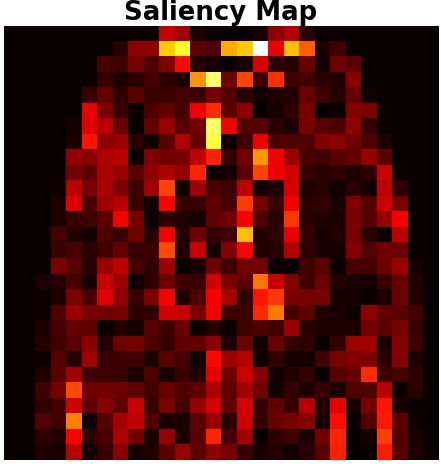
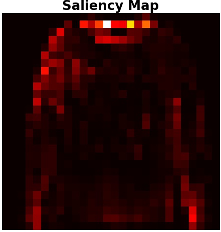
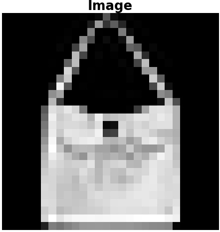
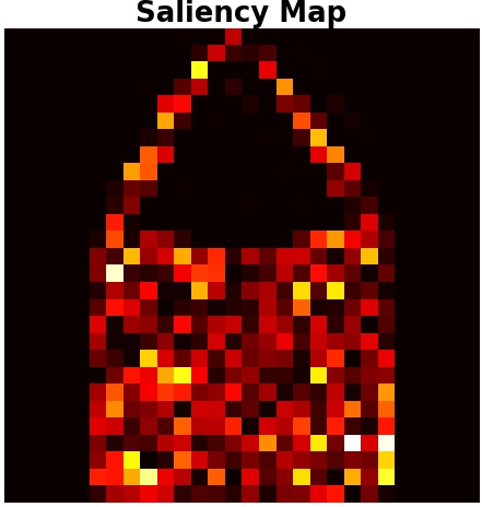
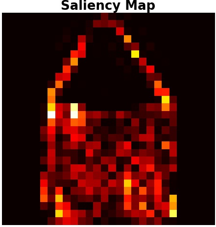
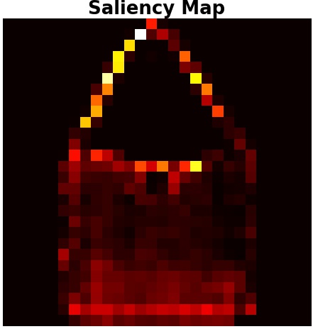
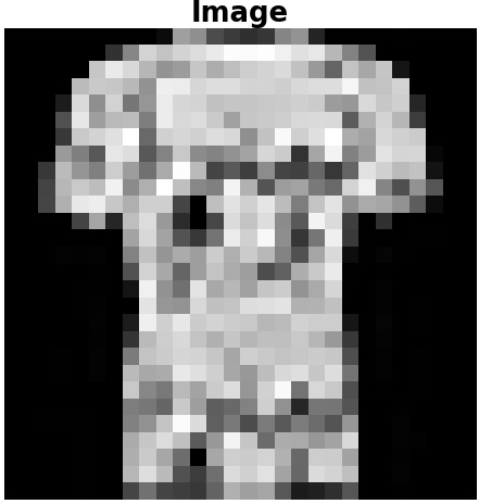
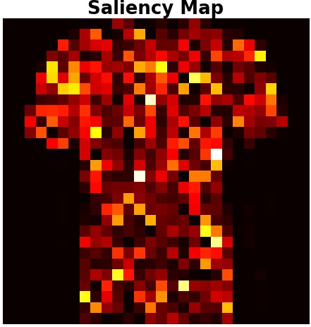
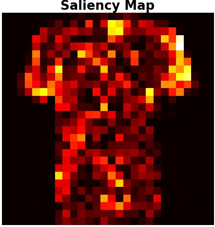
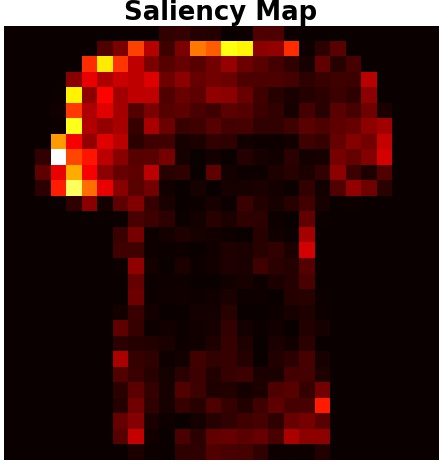
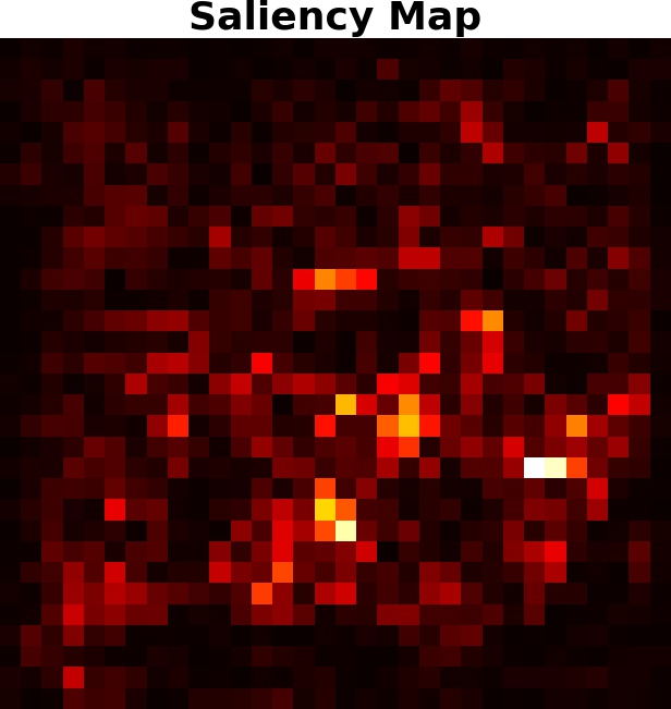
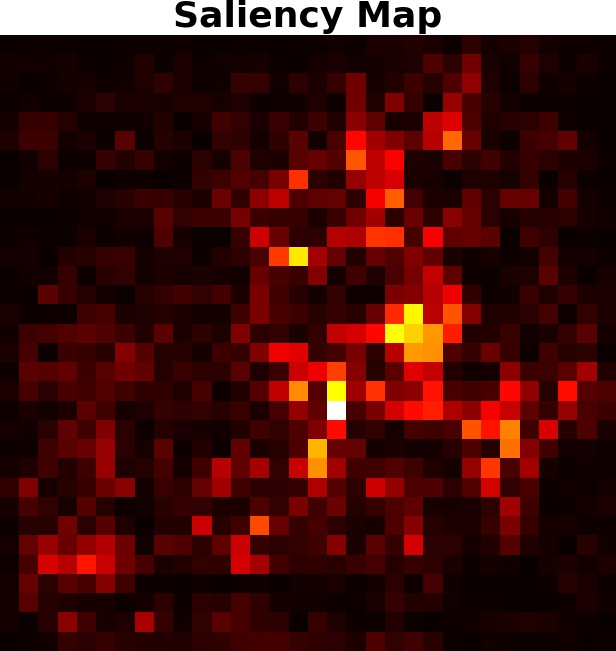
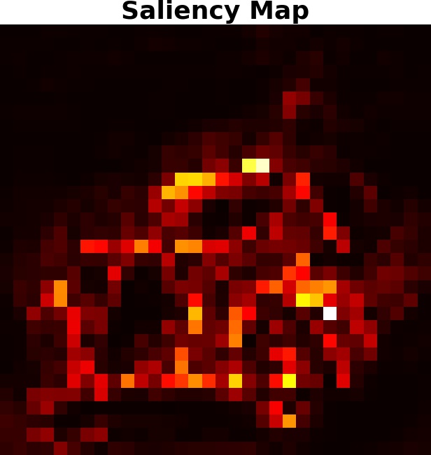
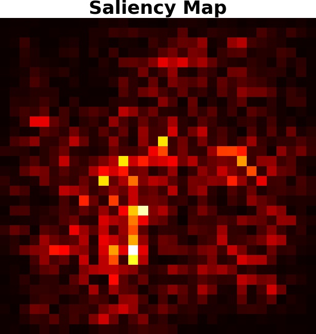
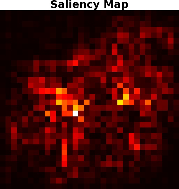
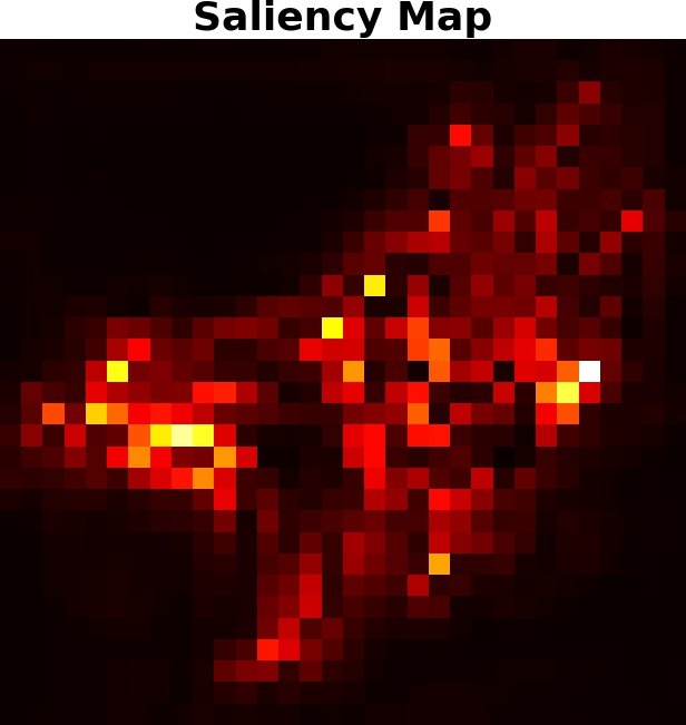
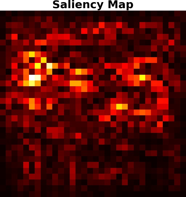
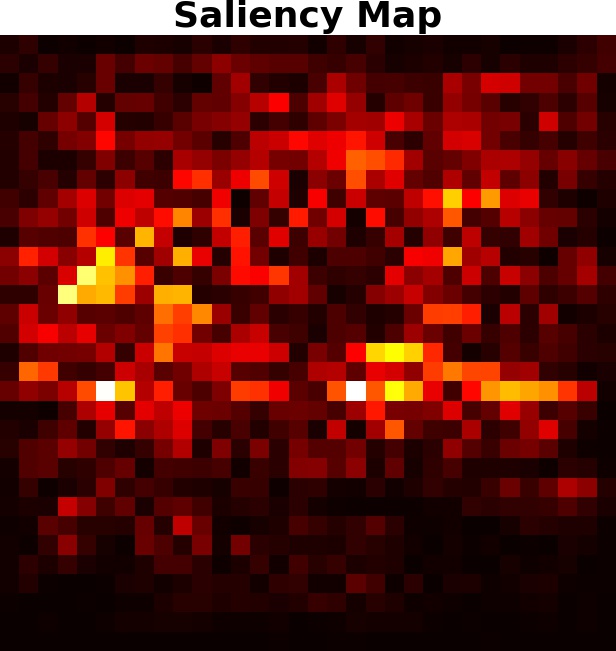
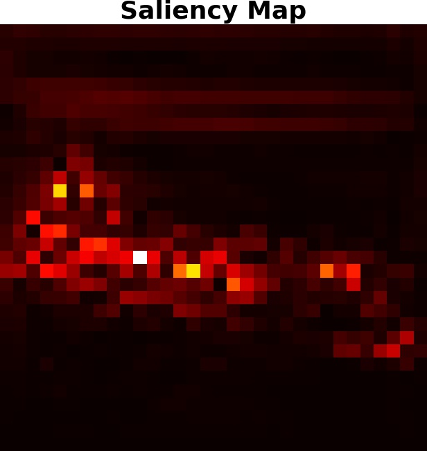
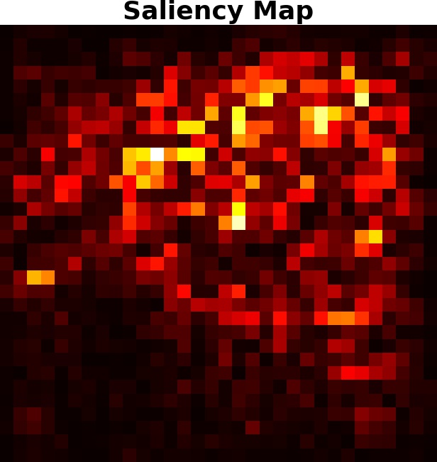
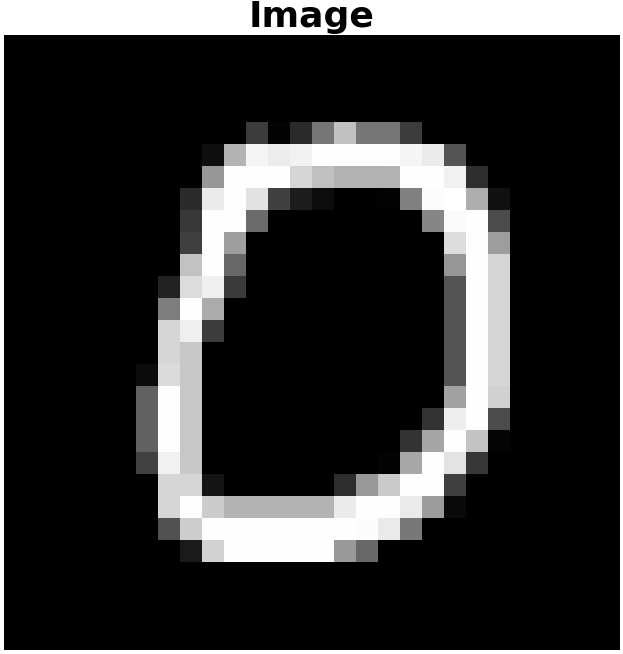
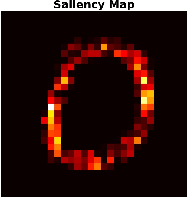
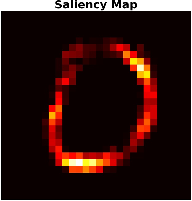
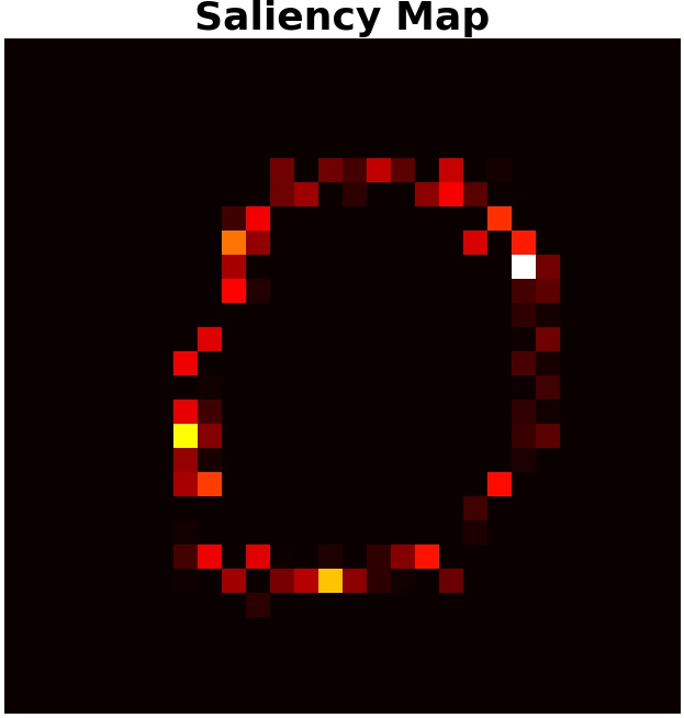
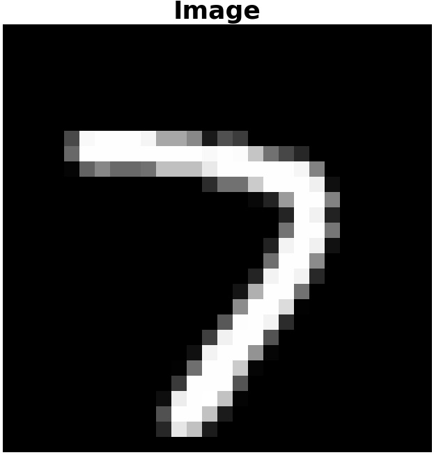
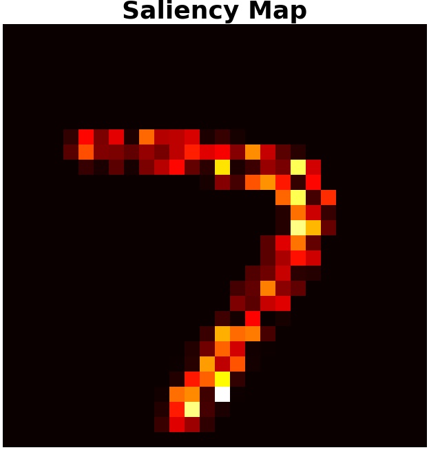
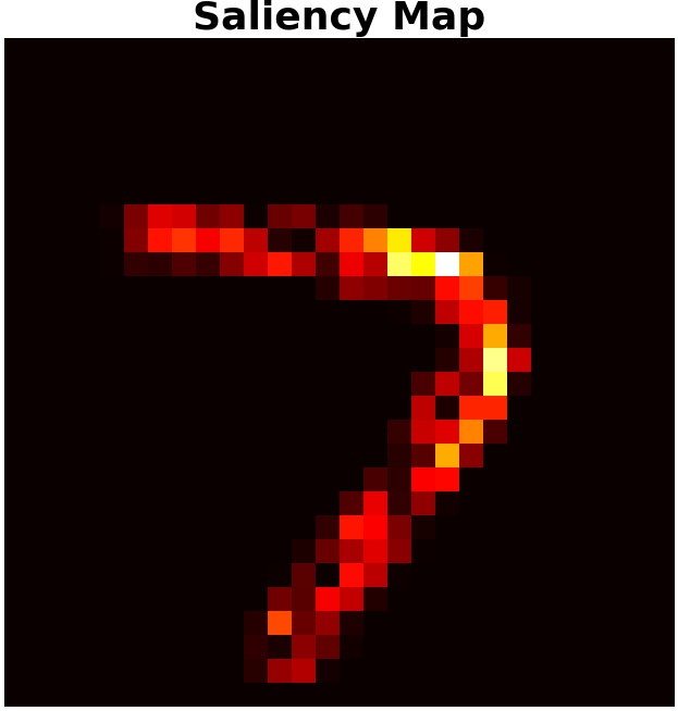
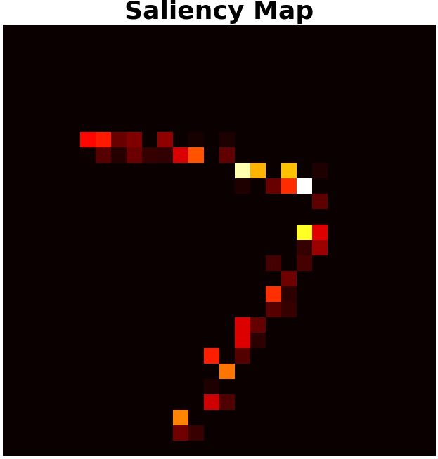
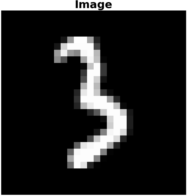
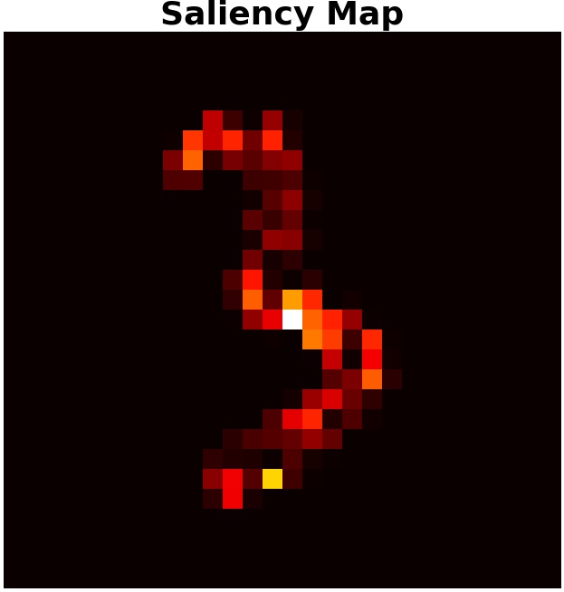
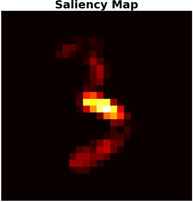
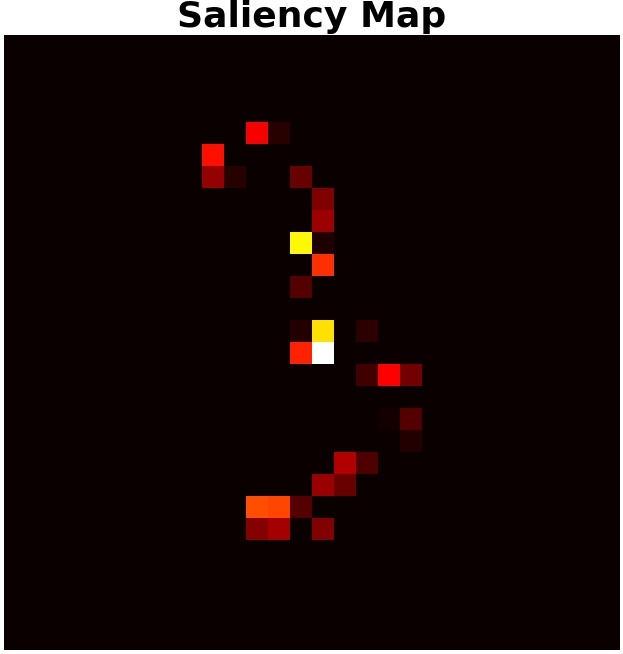
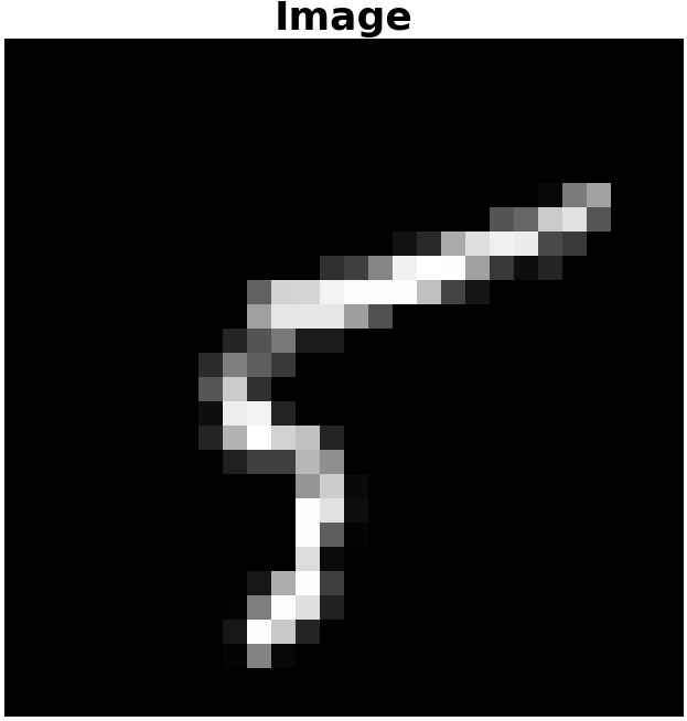
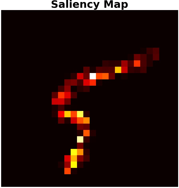
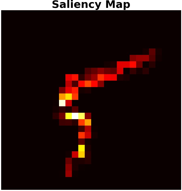
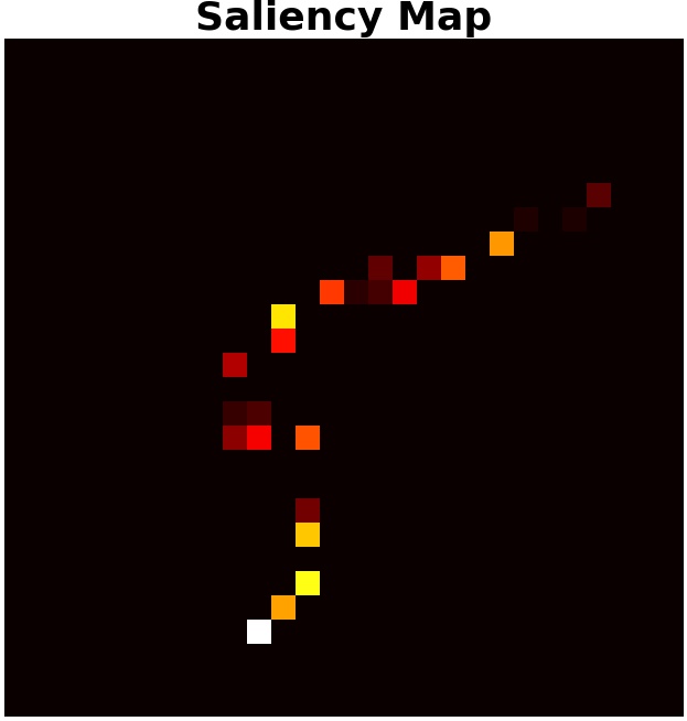
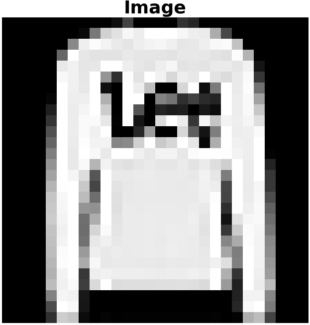
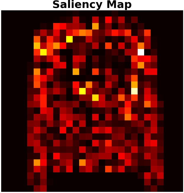
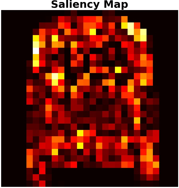
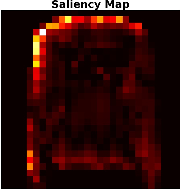
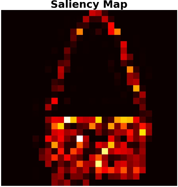
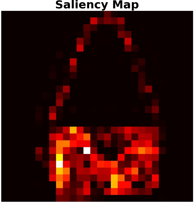
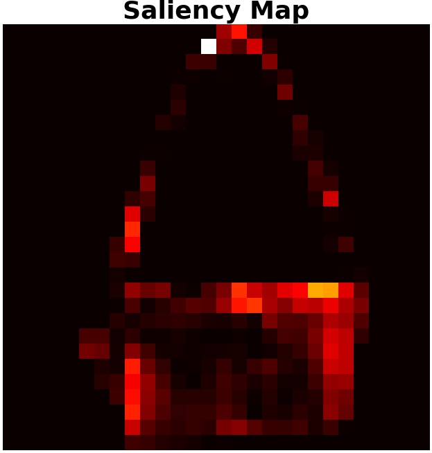
Empirically Demonstrate Attribution Sparseness: In Section 6 we empirically demonstrate that this “sparsification” effect of (ε)subscript𝜀\ell_{\infty}(\varepsilon)-adversarial training holds not only for 1-layer networks (e.g. logistic regression models), but also for Deep Convolutional Networks used for image classification, and extends beyond IG-based attributions, to those based on DeepSHAP. Specifically, we show this phenomenon via experiments applying (ε)subscript𝜀\ell_{\infty}(\varepsilon)-adversarial training to (a) Convolutional Neural Networks on public benchmark image datasets MNIST (LeCun & Cortes, 2010) and Fashion-MNIST (Xiao et al., 2017), and (b) logistic regression models on the Mushroom and Spambase tabular datasets from the UCI Data Repository (Dheeru & Karra Taniskidou, 2017). In all of our experiments, we find that it is possible to choose an subscript\ell_{\infty} bound ε𝜀\varepsilon so that adversarial learning under this bound produces attribution vectors that are sparse on average, with little or no drop in performance on natural test data. A visually striking example of this effect is shown in Figure 2 (the Gini Index, introduced in Section 6, measures the sparseness of the map).

It is natural to wonder whether a traditional weight-regularization technique such as 1subscript1\ell_{1}-regularization can produce models with sparse attribution vectors. In fact, our experiments show that for logistic regression models, 1subscript1\ell_{1}-regularized training does yield attribution vectors that are on average significantly sparser compared to attribution vectors from natural (un-regularized) model-training, and the sparseness improvement is almost as good as that obtained with (ε)subscript𝜀\ell_{\infty}(\varepsilon)-adversarial training. This is not too surprising given our result (Lemma 4.1) that implies a direct link between sparseness of weights and sparseness of IG vectors, for 1-layer models. Intriguingly, this does not carry over to DNNs: for multi-layer models (such as the ConvNets we trained for the image datasets mentioned above) we find that with 1subscript1\ell_{1}-regularization, the sparseness improvement is significantly inferior to that obtainable from (ε)subscript𝜀\ell_{\infty}(\varepsilon)-adversarial training (when controlling for model accuracy on natural test data), as we show in Table 1, Figure 3 and Figure 4. Thus it appears that for DNNs, the attribution-sparseness that results from adversarial training is not necessarily related to sparseness of weights.

Connection between Adversarial Training and Attribution Stability: We also show theoretically (Section 5) that training 1-layer networks naturally, while encouraging stability of explanations (via a suitable term added to the loss function), is in fact equivalent to adversarial training.

Natural Training       Adversarial Training

Refer to caption
Refer to caption
Gini: 0.6150
Refer to caption
Gini: 0.7084
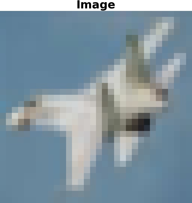
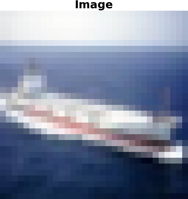
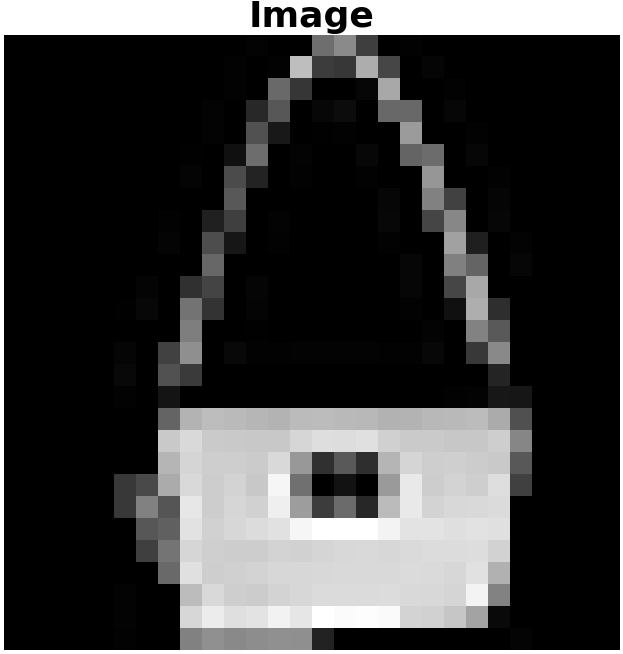
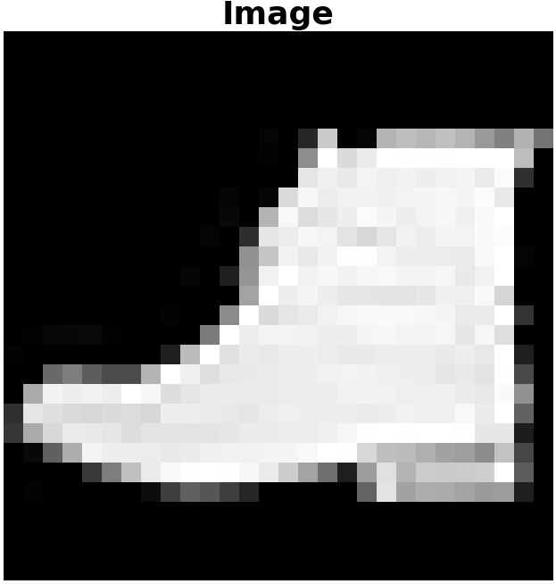
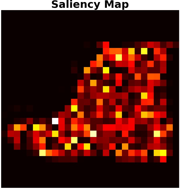
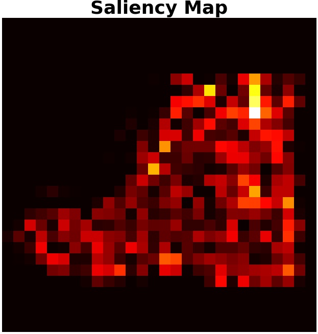
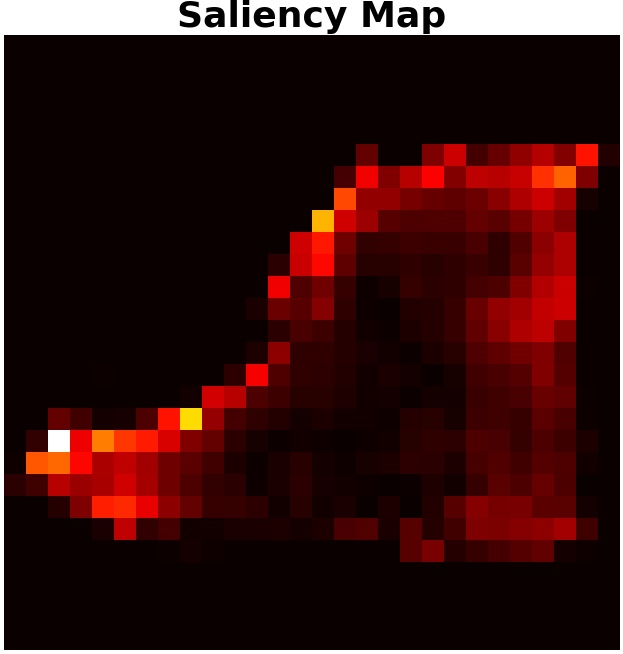
Figure 2: Both models correctly predict “Bird”, but the IG-based saliency map of the adversarially trained model is much sparser than that of the naturally trained model.

2 Setup and Assumptions

For ease of understanding, we consider the case of binary classification for the rest of our discussion in the main paper. We assume there is a distribution 𝒟𝒟\mathcal{D} of data points (𝐱,y)𝐱𝑦(\operatorname{{\boldsymbol{x}}},y) where 𝐱d𝐱superscript𝑑\operatorname{{\boldsymbol{x}}}\in\mathbb{R}^{d} is an input feature vector, and y{±1}𝑦plus-or-minus1y\in\{\pm 1\} is its true label111It is trivial to convert -1/1 labels to 0/1 labels and vice versa. For each i[d]𝑖delimited-[]𝑑i\in[d], the i𝑖i’th component of 𝐱𝐱\operatorname{{\boldsymbol{x}}} represents an input feature, and is denoted by xisubscript𝑥𝑖x_{i}. The model is assumed to have learnable parameters (“weights”) 𝐰d𝐰superscript𝑑\operatorname{{\boldsymbol{w}}}\in\mathbb{R}^{d}, and for a given data point (𝐱,y)𝐱𝑦(\operatorname{{\boldsymbol{x}}},y), the loss is given by some function (𝐱,y;𝐰)𝐱𝑦𝐰\mathcal{L}(\operatorname{{\boldsymbol{x}}},y;\operatorname{{\boldsymbol{w}}}). Natural model training 222Also referred to as standard training by (Madry et al., 2017) consists of minimizing the expected loss, known as empirical risk:

𝔼(𝐱,y)𝒟[(𝐱,y;𝐰)].subscript𝔼similar-to𝐱𝑦𝒟delimited-[]𝐱𝑦𝐰\mathbb{E}_{(\operatorname{{\boldsymbol{x}}},y)\sim\operatorname{{\cal D}}}[\mathcal{L}(\operatorname{{\boldsymbol{x}}},y;\operatorname{{\boldsymbol{w}}})]. (1)

We sometimes assume the existence of an (ε)subscript𝜀\ell_{\infty}(\varepsilon)-adversary who may perturb the input example 𝐱𝐱\operatorname{{\boldsymbol{x}}} by adding a vector δd𝛿superscript𝑑\delta\in\mathbb{R}^{d} whose subscript\ell_{\infty}-norm is bounded by ε𝜀\varepsilon; such a perturbation δ𝛿\delta is referred to as an (ε)subscript𝜀\ell_{\infty}(\varepsilon)-perturbation. For a given data point (𝐱,y)𝐱𝑦(\operatorname{{\boldsymbol{x}}},y) and a given loss function (.)\mathcal{L}(.), an (ε)subscript𝜀\ell_{\infty}(\varepsilon)-adversarial perturbation is a δsuperscript𝛿\delta^{*} that maximizes the adversarial loss (𝐱+δ,y;𝐰)𝐱superscript𝛿𝑦𝐰\mathcal{L}(\operatorname{{\boldsymbol{x}}}+\delta^{*},y;\operatorname{{\boldsymbol{w}}}).

Given a function F:d[0,1]:𝐹superscript𝑑01F:\operatorname{{\mathbb{R}}}^{d}\rightarrow[0,1] representing a neural network, an input vector 𝐱d𝐱superscript𝑑\operatorname{{\boldsymbol{x}}}\in\operatorname{{\mathbb{R}}}^{d}, and a suitable baseline vector 𝐮d𝐮superscript𝑑\operatorname{{\boldsymbol{u}}}\in\operatorname{{\mathbb{R}}}^{d}, an attribution of the prediction of F𝐹F at input 𝐱𝐱\operatorname{{\boldsymbol{x}}} relative to 𝐮𝐮\operatorname{{\boldsymbol{u}}} is a vector AF(𝐱,𝐮)dsuperscript𝐴𝐹𝐱𝐮superscript𝑑A^{F}(\operatorname{{\boldsymbol{x}}},\operatorname{{\boldsymbol{u}}})\in\operatorname{{\mathbb{R}}}^{d} whose i𝑖i’th component AiF(𝐱,𝐮)superscriptsubscript𝐴𝑖𝐹𝐱𝐮A_{i}^{F}(\operatorname{{\boldsymbol{x}}},\operatorname{{\boldsymbol{u}}}) represents the “contribution” of xisubscript𝑥𝑖x_{i} to the prediction F(𝐱)𝐹𝐱F(\operatorname{{\boldsymbol{x}}}). A variety of attribution methods have been proposed in the literature (see (Arya et al., 2019) for a survey), but in this paper we will focus on two of the most popular ones: Integrated Gradients (Sundararajan et al., 2017), and DeepSHAP (Lundberg & Lee, 2017). When discussing a specific attribution method, we will denote the IG-based attribution vector as IGF(𝐱,𝐮)superscriptIG𝐹𝐱𝐮\operatorname{IG}^{F}(\operatorname{{\boldsymbol{x}}},\operatorname{{\boldsymbol{u}}}), and the DeepSHAP-based attribution vector as SHF(𝐱,𝐮)superscriptSH𝐹𝐱𝐮\operatorname{SH}^{F}(\operatorname{{\boldsymbol{x}}},\operatorname{{\boldsymbol{u}}}). In all cases we will drop the superscript F𝐹F and/or the baseline vector 𝐮𝐮\operatorname{{\boldsymbol{u}}} when those are clear from the context.

The aim of adversarial training(Madry et al., 2017) is to train a model that is robust to an (ε)subscript𝜀\ell_{\infty}(\varepsilon)-adversary (i.e. performs well in the presence of such an adversary), and consists of minimizing the expected (ε)subscript𝜀\ell_{\infty}(\varepsilon)-adversarial loss:

𝔼(𝐱,y)𝒟[maxδε(𝐱+δ,y;𝐰)].subscript𝔼similar-to𝐱𝑦𝒟delimited-[]subscriptsubscriptnorm𝛿𝜀𝐱𝛿𝑦𝐰\mathbb{E}_{(\operatorname{{\boldsymbol{x}}},y)\sim\operatorname{{\cal D}}}[\max_{||\delta||_{\infty}\leq\varepsilon}\mathcal{L}(\operatorname{{\boldsymbol{x}}}+\delta,y;\operatorname{{\boldsymbol{w}}})]. (2)

In the expectations (1) and (2) we often drop the subscript under 𝔼𝔼\mathbb{E} when it is clear that the expectation is over (𝐱,y)𝒟similar-to𝐱𝑦𝒟(\operatorname{{\boldsymbol{x}}},y)\sim\operatorname{{\cal D}}.

Some of our theoretical results make assumptions regarding the form and properties of the loss function \mathcal{L}, the properties of its first derivative. For the sake of clarify, we highlight these assumptions (with mnemonic names) here for ease of future reference.

Assumption LOSS-INC.

The loss function is of the form (𝐱,y;𝐰)=g(y𝐰,𝐱)𝐱𝑦𝐰𝑔𝑦𝐰𝐱\mathcal{L}(\operatorname{{\boldsymbol{x}}},y;\operatorname{{\boldsymbol{w}}})=g(-y\langle\operatorname{{\boldsymbol{w}}},\operatorname{{\boldsymbol{x}}}\rangle) where g𝑔g is a non-decreasing function.

Assumption LOSS-CVX.

The loss function is of the form (𝐱,y;𝐰)=g(y𝐰,𝐱)𝐱𝑦𝐰𝑔𝑦𝐰𝐱\mathcal{L}(\operatorname{{\boldsymbol{x}}},y;\operatorname{{\boldsymbol{w}}})=g(-y\langle\operatorname{{\boldsymbol{w}}},\operatorname{{\boldsymbol{x}}}\rangle) where g𝑔g is non-decreasing, almost-everywhere differentiable, and convex.

Section B.1 in the Supplement shows that these Assumptions are satisfied by popular loss functions such as logistic and hinge loss. Incidentally, note that for any differentiable function g𝑔g, g𝑔g is convex if and only if its first-derivative gsuperscript𝑔g^{\prime} is non-decreasing, and we will use this property in some of the proofs.

Assumption FEAT-TRANS.

For each i[d]𝑖delimited-[]𝑑i\in[d], if xisubscriptsuperscript𝑥𝑖x^{\prime}_{i} is the feature in the original dataset, xisubscript𝑥𝑖x_{i} is the translated version of xisubscriptsuperscript𝑥𝑖x^{\prime}_{i} defined by xi=xi[E(xi|y=1)+E(xi|y=1)]/2subscript𝑥𝑖subscriptsuperscript𝑥𝑖delimited-[]𝐸conditionalsubscriptsuperscript𝑥𝑖𝑦1𝐸conditionalsubscriptsuperscript𝑥𝑖𝑦12x_{i}=x^{\prime}_{i}-[E(x^{\prime}_{i}|y=1)+E(x^{\prime}_{i}|y=-1)]/2.

In Section B.2 (Supplement) we show that this mild assumption implies that for each feature xisubscript𝑥𝑖x_{i} there is a constant aisubscript𝑎𝑖a_{i} such that

𝔼(xi|y)𝔼conditionalsubscript𝑥𝑖𝑦\displaystyle\mathbb{E}(x_{i}|y) =aiyabsentsubscript𝑎𝑖𝑦\displaystyle=a_{i}y (3)
𝔼(yxi)𝔼𝑦subscript𝑥𝑖\displaystyle\mathbb{E}(yx_{i}) =𝔼[𝔼(yxi|y)]=𝔼[y2ai]=aiabsent𝔼delimited-[]𝔼conditional𝑦subscript𝑥𝑖𝑦𝔼delimited-[]superscript𝑦2subscript𝑎𝑖subscript𝑎𝑖\displaystyle=\mathbb{E}[\mathbb{E}(yx_{i}|y)]=\mathbb{E}[y^{2}a_{i}]=a_{i} (4)
𝔼(yxi|y)𝔼conditional𝑦subscript𝑥𝑖𝑦\displaystyle\mathbb{E}(yx_{i}|y) =y𝔼[xi|y]=y2ai=aiabsent𝑦𝔼delimited-[]conditionalsubscript𝑥𝑖𝑦superscript𝑦2subscript𝑎𝑖subscript𝑎𝑖\displaystyle=y\mathbb{E}[x_{i}|y]=y^{2}a_{i}=a_{i} (5)

For any i[d]𝑖delimited-[]𝑑i\in[d], we can think of 𝔼(yxi)𝔼𝑦subscript𝑥𝑖\mathbb{E}(yx_{i}) as the degree of association333When the features are standardized to have mean 0, 𝔼(yxi)𝔼𝑦subscript𝑥𝑖\mathbb{E}(yx_{i}) is in fact the covariance of y𝑦y and xisubscript𝑥𝑖x_{i}. between feature xisubscript𝑥𝑖x_{i} and label y𝑦y. Since 𝔼(yxi)=ai𝔼𝑦subscript𝑥𝑖subscript𝑎𝑖\mathbb{E}(yx_{i})=a_{i} (Eq. 4), we refer to aisubscript𝑎𝑖a_{i} as the directed strength444This is related to the feature “robustness” notion introduced in (Ilyas et al., 2019) of feature xisubscript𝑥𝑖x_{i}, and |ai|subscript𝑎𝑖|a_{i}| is referred to as the absolute strength of xisubscript𝑥𝑖x_{i}. In particular when |ai|subscript𝑎𝑖|a_{i}| is large (small) we say that xisubscript𝑥𝑖x_{i} is a strong (weak) feature.

2.1 Averaging over a group of features

For our main theoretical result (Theorem 3.1), we need a notion of weighted average defined as follows:

Definition WTD-AV.

Given a quantity qisubscript𝑞𝑖q_{i} defined for each feature-index i[d]𝑖delimited-[]𝑑i\in[d], a subset S[d]𝑆delimited-[]𝑑S\subset[d] (where |S|1𝑆1|S|\geq 1) of feature-indices, and a feature weight-vector 𝐰𝐰\mathbf{w} with wi0subscript𝑤𝑖0w_{i}\neq 0 for at least one iS𝑖𝑆i\in S, the 𝐰𝐰\mathbf{w}-weighted average of qqq over SSS is defined as

qS𝐰:=iSwiqiiS|wi|assignsubscriptsuperscript𝑞𝐰𝑆subscript𝑖𝑆subscript𝑤𝑖subscript𝑞𝑖subscript𝑖𝑆subscript𝑤𝑖q^{\mathbf{w}}_{S}:=\frac{\sum_{i\in S}w_{i}q_{i}}{\sum_{i\in S}|w_{i}|} (6)

Note that the quantity wiqisubscript𝑤𝑖subscript𝑞𝑖w_{i}q_{i} can be written as |wi|sgn(wi)qisubscript𝑤𝑖sgnsubscript𝑤𝑖subscript𝑞𝑖|w_{i}|\operatorname{sgn}(w_{i})q_{i}, so qS𝐰subscriptsuperscript𝑞𝐰𝑆q^{\mathbf{w}}_{S} is essentially a |wi|subscript𝑤𝑖|w_{i}|-weighted average of sgn(wi)qisgnsubscript𝑤𝑖subscript𝑞𝑖\operatorname{sgn}(w_{i})q_{i} over iS𝑖𝑆i\in S.

For our result we will use the above 𝐰𝐰\mathbf{w}-weighted average definition for two particular quantities qisubscript𝑞𝑖q_{i}. The first one is qi:=aiassignsubscript𝑞𝑖subscript𝑎𝑖q_{i}:=a_{i}, the directed strength of feature xisubscript𝑥𝑖x_{i} (Eq. 4). Intuitively, the quantity sgn(wi)𝔼(yxi)=aisgn(wi)sgnsubscript𝑤𝑖𝔼𝑦subscript𝑥𝑖subscript𝑎𝑖sgnsubscript𝑤𝑖\operatorname{sgn}(w_{i})\mathbb{E}(yx_{i})=a_{i}\operatorname{sgn}(w_{i}) captures the aligned strength of feature xisubscript𝑥𝑖x_{i} in the following sense: if this quantity is large and positive (large and negative), it indicates both that the current weight wisubscript𝑤𝑖w_{i} of xisubscript𝑥𝑖x_{i} is aligned (misaligned) with the directed strength of xisubscript𝑥𝑖x_{i}, and that this directed strength is large. Thus aS𝐰subscriptsuperscript𝑎𝐰𝑆a^{\mathbf{w}}_{S} represents an average of the aligned strength over the feature-group S𝑆S.

The second quantity for which we define the above 𝐰𝐰\mathbf{w}-weighted average is qi:=Δ¯iassignsubscript𝑞𝑖subscript¯Δ𝑖q_{i}:=\overline{\Delta}_{i}, where Δ¯i:=𝔼[/wi]assignsubscript¯Δ𝑖𝔼delimited-[]subscript𝑤𝑖\overline{\Delta}_{i}:=-\mathbb{E}[\partial\mathcal{L}/\partial w_{i}] represents the expected SGD update (over random draws from the data distribution) of the weight wisubscript𝑤𝑖w_{i}, given the loss function \mathcal{L}, for a unit learning rate (details are in the next Section). The quantity sgn(wi)Δ¯isgnsubscript𝑤𝑖subscript¯Δ𝑖\operatorname{sgn}(w_{i})\overline{\Delta}_{i} has a natural interpretation, analogous to the above interpretation of aisgn(wi)subscript𝑎𝑖sgnsubscript𝑤𝑖a_{i}\operatorname{sgn}(w_{i}): a large positive (large negative) value of sgn(wi)Δ¯isgnsubscript𝑤𝑖subscript¯Δ𝑖\operatorname{sgn}(w_{i})\overline{\Delta}_{i} corresponds to an large expansion (large shrinkage), in expectation, of the weight wisubscript𝑤𝑖w_{i} away from zero magnitude (toward zero magnitude). Thus the 𝐰𝐰\mathbf{w}-weighted average Δ¯S𝐰subscriptsuperscript¯Δ𝐰𝑆\overline{\Delta}^{\mathbf{w}}_{S} represents the |wi|subscript𝑤𝑖|w_{i}|-weighted average of this effect over the feature-group S𝑆S.

3 Analysis of SGD Updates in Adversarial Training

One way to understand the characteristics of the weights in an adversarially-trained neural network model, is to analyze how the weights evolve during adversarial training under Stochastic Gradient Descent (SGD) optimization. One of the main results of this work is a theoretical characterization of the weight updates during a single SGD step, when applied to a randomly drawn data point (𝐱,y)𝒟similar-to𝐱𝑦𝒟(\operatorname{{\boldsymbol{x}}},y)\sim\operatorname{{\cal D}} that is subjected to an (ε)subscript𝜀\ell_{\infty}(\varepsilon)-adversarial perturbation.

Although the holy grail would be to do this for general DNNs (and we expect this will be quite difficult) we take a first step in this direction by analyzing single-layer networks for binary or multi-class classification, where each weight is associated with an input feature. Intriguingly, our results (Theorem 3.1 for binary classification and E.1 for multi-class classification in the Supplement) show that for these models, (ε)subscript𝜀\ell_{\infty}(\varepsilon)-adversarial training tends to selectively reduce the weight-magnitude of weakly relevant or irrelevant features, and does so much more aggressively than natural training. In other words, natural training can result in models where many weak features have significant weights, whereas adversarial training would tend to push most of these weights close to zero. The resulting model weights would thus be more sparse, and the corresponding IG-based attribution vectors would on average be more sparse as well (since in linear models, sparse weights imply sparse IG vectors; this is a consequence of Lemma 4.1) compared to naturally-trained models.

Our experiments (Sec. 6) show that indeed for logistic regression models (which satisfy the conditions of Theorem 3.1), adversarial training leads to sparse IG vectors. Interestingly, our extensive experiments with Deep Convolutional Neural Networks on public image datasets demonstrate that this phenomenon extends to DNNs as well, and to attributions based on DeepSHAP, even though our theoretical results only apply to 1-layer networks and IG-based attributions.

As a preliminary, it is easy to show the following expressions related to the (ε)subscript𝜀\ell_{\infty}(\varepsilon)-adversarial perturbation δsuperscript𝛿\delta^{*} (See Lemmas 2 and 3 in Section C of the Supplement): For loss functions satisfying Assumption LOSS-INC, the (ε)subscript𝜀\ell_{\infty}(\varepsilon)-adversarial perturbation δsuperscript𝛿\delta^{*} is given by:

δ=ysgn(𝐰)ε,superscript𝛿𝑦sgn𝐰𝜀\delta^{*}=-y\operatorname{sgn}(\operatorname{{\boldsymbol{w}}})\varepsilon, (7)

the corresponding (ε)subscript𝜀\ell_{\infty}(\varepsilon)-adversarial loss is

(𝐱+δ,y;𝐰)=g(ε𝐰1y𝐰,𝐱),𝐱superscript𝛿𝑦𝐰𝑔𝜀subscriptnorm𝐰1𝑦𝐰𝐱\mathcal{L}(\operatorname{{\boldsymbol{x}}}+\delta^{*},y;\;\operatorname{{\boldsymbol{w}}})=g(\varepsilon||\operatorname{{\boldsymbol{w}}}||_{1}-y\langle\operatorname{{\boldsymbol{w}}},\,\operatorname{{\boldsymbol{x}}}\rangle), (8)

and the gradient of this loss w.r.t. a weight wisubscript𝑤𝑖w_{i} is

(𝐱+δ,y;𝐰)wi=g(ε𝐰1y𝐰,𝐱)(yxisgn(wi)ε).𝐱superscript𝛿𝑦𝐰subscript𝑤𝑖superscript𝑔𝜀subscriptnorm𝐰1𝑦𝐰𝐱𝑦subscript𝑥𝑖sgnsubscript𝑤𝑖𝜀\frac{\partial\mathcal{L}(\operatorname{{\boldsymbol{x}}}+\delta^{*},y;\;\operatorname{{\boldsymbol{w}}})}{\partial w_{i}}=\\ -g^{\prime}(\varepsilon||\operatorname{{\boldsymbol{w}}}||_{1}-y\langle\operatorname{{\boldsymbol{w}}},\operatorname{{\boldsymbol{x}}}\rangle)\;(yx_{i}-\operatorname{sgn}(w_{i})\varepsilon). (9)

In our main result, the expectation of the gsuperscript𝑔g^{\prime} term in (9) plays an important role, so we will use the following notation:

g¯:=𝔼[g(ε𝐰1y𝐰,𝐱)],assign¯superscript𝑔𝔼delimited-[]superscript𝑔𝜀subscriptnorm𝐰1𝑦𝐰𝐱\overline{g^{\prime}}:=\mathbb{E}\big{[}g^{\prime}(\varepsilon||\operatorname{{\boldsymbol{w}}}||_{1}-y\langle\operatorname{{\boldsymbol{w}}},\operatorname{{\boldsymbol{x}}}\rangle)\big{]}, (10)

and by Assumption LOSS-INC, g¯¯superscript𝑔\overline{g^{\prime}} is non-negative.

Ideally, we would like to understand the nature of the weight-vector 𝐰superscript𝐰\operatorname{{\boldsymbol{w}}}^{*} that minimizes the expected adversarial loss (2). This is quite challenging, so rather than analyzing the final optimum of (2), we instead analyze how an SGD-based optimizer for (2) updates the model weights 𝐰𝐰\operatorname{{\boldsymbol{w}}}. We assume an idealized SGD process: (a) a data point (𝐱,y)𝐱𝑦(\operatorname{{\boldsymbol{x}}},y) is drawn from distribution 𝒟𝒟\operatorname{{\cal D}}, (b) 𝐱𝐱\operatorname{{\boldsymbol{x}}} is replaced by 𝐱=𝐱+δsuperscript𝐱𝐱superscript𝛿\operatorname{{\boldsymbol{x}}}^{\prime}=\operatorname{{\boldsymbol{x}}}+\delta^{*} where δsuperscript𝛿\delta^{*} is an (ε)subscript𝜀\ell_{\infty}(\varepsilon)-adversarial perturbation with respect to the loss function \mathcal{L}, (c) each weight wisubscript𝑤𝑖w_{i} is updated by an amount Δwi=(𝐱,y;𝐰)/wiΔsubscript𝑤𝑖superscript𝐱𝑦𝐰subscript𝑤𝑖\Delta w_{i}=-\partial\mathcal{L}(\operatorname{{\boldsymbol{x}}}^{\prime},y;\operatorname{{\boldsymbol{w}}})/\partial w_{i} (assuming a unit learning rate to avoid notational clutter). We are interested in the expectation Δ¯i:=𝔼Δwi=𝔼[(𝐱,y;𝐰)/wi]assignsubscript¯Δ𝑖𝔼Δsubscript𝑤𝑖𝔼delimited-[]superscript𝐱𝑦𝐰subscript𝑤𝑖\overline{\Delta}_{i}:=\mathbb{E}\Delta w_{i}=-\mathbb{E}[\partial\mathcal{L}(\operatorname{{\boldsymbol{x}}}^{\prime},y;\mathbf{w})/\partial w_{i}], in order to understand how a weight wisubscript𝑤𝑖w_{i} evolves on average during a single SGD step. Where there is a conditionally independent feature subset S[d]𝑆delimited-[]𝑑S\in[d] (i.e. the features in S𝑆S are conditionally independent of the rest given the label y𝑦y), our main theoretical result characterizes the behavior of Δ¯isubscript¯Δ𝑖\overline{\Delta}_{i} for iS𝑖𝑆i\in S, and the corresponding 𝐰𝐰\mathbf{w}-weighted average Δ¯S𝐰subscriptsuperscript¯Δ𝐰𝑆\overline{\Delta}^{\mathbf{w}}_{S}:

Theorem 3.1 (Expected SGD Update in Adversarial Training).

For any loss function \mathcal{L} satisfying Assumption LOSS-CVX, a dataset 𝒟𝒟\operatorname{{\cal D}} satisfying Assumption FEAT-TRANS, a subset S𝑆S of features that are conditionally independent of the rest given the label y𝑦y, if a data point (𝐱,y)𝐱𝑦(\operatorname{{\boldsymbol{x}}},y) is randomly drawn from 𝒟𝒟\operatorname{{\cal D}}, and 𝐱𝐱\operatorname{{\boldsymbol{x}}} is perturbed to 𝐱=𝐱+δsuperscript𝐱𝐱superscript𝛿\operatorname{{\boldsymbol{x}}}^{\prime}=\operatorname{{\boldsymbol{x}}}+\delta^{*}, where δsuperscript𝛿\delta^{*} is an (ε)subscript𝜀\ell_{\infty}(\varepsilon)-adversarial perturbation, then during SGD using the (ε)subscript𝜀\ell_{\infty}(\varepsilon)-adversarial loss (𝐱,y;𝐰)superscript𝐱𝑦𝐰\mathcal{L}(\operatorname{{\boldsymbol{x}}}^{\prime},y;\operatorname{{\boldsymbol{w}}}), the expected weight-updates Δ¯i:=𝔼Δwiassignsubscript¯Δ𝑖𝔼Δsubscript𝑤𝑖\overline{\Delta}_{i}:=\mathbb{E}\Delta w_{i} for iS𝑖𝑆i\in S and the corresponding 𝐰𝐰\mathbf{w}-weighted average Δ¯S𝐰subscriptsuperscript¯Δ𝐰𝑆\overline{\Delta}^{\mathbf{w}}_{S} satisfy the following properties:

  1. 1.

    If wi=0iSsubscript𝑤𝑖0for-all𝑖𝑆w_{i}=0\;\forall i\in S, then for each iS𝑖𝑆i\in S,

    Δ¯i=g¯ai,subscript¯Δ𝑖¯superscript𝑔subscript𝑎𝑖\overline{\Delta}_{i}=\overline{g^{\prime}}\;a_{i}, (11)
  2. 2.

    and otherwise,

    Δ¯S𝐰g¯(aS𝐰ε),subscriptsuperscript¯Δ𝐰𝑆¯superscript𝑔subscriptsuperscript𝑎𝐰𝑆𝜀\overline{\Delta}^{\mathbf{w}}_{S}\leq\overline{g^{\prime}}(a^{\mathbf{w}}_{S}-\varepsilon), (12)

    and equality holds in the limit as wi0iSsubscript𝑤𝑖0for-all𝑖𝑆w_{i}\rightarrow 0\;\forall i\in S,

where g¯¯superscript𝑔\overline{g^{\prime}} is the expectation in (10), ai=𝔼(xiy)subscript𝑎𝑖𝔼subscript𝑥𝑖𝑦a_{i}=\mathbb{E}(x_{i}y) is the directed strength of feature xisubscript𝑥𝑖x_{i} from Eq. (4), and aS𝐰subscriptsuperscript𝑎𝐰𝑆a^{\mathbf{w}}_{S} is the corresponding 𝐰𝐰\mathbf{w}-weighted average over S𝑆S.

For space reasons, a detailed discussion of the implications of this result is presented in Sec. D.2 of the Supplement, but here we note the following. Recalling the interpretation of the 𝐰𝐰\mathbf{w}-weighted averages aS𝐰subscriptsuperscript𝑎𝐰𝑆a^{\mathbf{w}}_{S} and Δ¯S𝐰subscriptsuperscript¯Δ𝐰𝑆\overline{\Delta}^{\mathbf{w}}_{S} in Section 2.1, we can interpret the above result as follows. For any conditionally independent feature subset S𝑆S, if the weights of all features in S𝑆S are zero, then by Eq. (11), an SGD update causes, on average, each of these weights wisubscript𝑤𝑖w_{i} to grow (from 0) in a direction consistent with the directed feature-strength aisubscript𝑎𝑖a_{i} (since g¯0¯superscript𝑔0\overline{g^{\prime}}\geq 0 as noted above). If at least one of the features in S𝑆S has a non-zero weight, (12) implies Δ¯S𝐰<0subscriptsuperscript¯Δ𝐰𝑆0\overline{\Delta}^{\mathbf{w}}_{S}<0, i.e., an aggregate shrinkage of the weights of features in S𝑆S, if either of the following hold: (a) aS𝐰<0subscriptsuperscript𝑎𝐰𝑆0a^{\mathbf{w}}_{S}<0, i.e., the weights of features in S𝑆S are mis-aligned on average, or (b) the weights of features in S𝑆S are aligned on average, i.e., aS𝐰subscriptsuperscript𝑎𝐰𝑆a^{\mathbf{w}}_{S} is positive, but dominated by ε𝜀\varepsilon, i.e. the features S𝑆S are weakly correlated with the label. In the latter case the weights of features in S𝑆S are (in aggregate and in expectation) aggressively pushed toward zero, and this aggressiveness is proportional to the extent to which ε𝜀\varepsilon dominates aS𝐰subscriptsuperscript𝑎𝐰𝑆a^{\mathbf{w}}_{S}. A partial generalization of the above result for the multi-class setting (for a single conditionally-independent feature) is presented in Section E (Theorem E.1) of the Supplement.

4 FEATURE ATTRIBUTION USING INTEGRATED GRADIENTS

Theorem 3.1 showed that (ε)subscript𝜀\ell_{\infty}(\varepsilon)-adversarial training tends to shrink the weights of features that are “weak” (relative to ε𝜀\varepsilon). We now show a link between weights and explanations, specifically explanations in the form of a vector of feature-attributions given by the Integrated Gradients (IG) method (Sundararajan et al., 2017), which is defined as follows: Suppose F:d:𝐹superscript𝑑F:\mathbb{R}^{d}\rightarrow\mathbb{R} is a real-valued function of an input vector. For example F𝐹F could represent the output of a neural network, or even a loss function (𝐱,y;𝐰)𝐱𝑦𝐰\mathcal{L}(\operatorname{{\boldsymbol{x}}},y;\operatorname{{\boldsymbol{w}}}) when the label y𝑦y and weights 𝐰𝐰\operatorname{{\boldsymbol{w}}} are held fixed. Let 𝐱d𝐱superscript𝑑\operatorname{{\boldsymbol{x}}}\in\mathbb{R}^{d} be a specific input, and 𝐮d𝐮superscript𝑑\operatorname{{\boldsymbol{u}}}\in\mathbb{R}^{d} be a baseline input. The IG is defined as the path integral of the gradients along the straight-line path from the baseline 𝐮𝐮\operatorname{{\boldsymbol{u}}} to the input 𝐱𝐱\operatorname{{\boldsymbol{x}}}. The IG along the i𝑖i’th dimension for an input 𝐱𝐱\operatorname{{\boldsymbol{x}}} and baseline 𝐮𝐮\operatorname{{\boldsymbol{u}}} is defined as:

IGiF(𝐱,𝐮):=(xiui)×α=01iF(𝐮+α(𝐱𝐮))dα,assignsuperscriptsubscriptIG𝑖𝐹𝐱𝐮subscript𝑥𝑖subscript𝑢𝑖superscriptsubscript𝛼01subscript𝑖𝐹𝐮𝛼𝐱𝐮𝑑𝛼\operatorname{IG}_{i}^{F}(\operatorname{{\boldsymbol{x}}},\operatorname{{\boldsymbol{u}}}):=(x_{i}-u_{i})\times\int_{\alpha=0}^{1}\partial_{i}F(\operatorname{{\boldsymbol{u}}}+\alpha(\operatorname{{\boldsymbol{x}}}-\operatorname{{\boldsymbol{u}}}))d\alpha, (13)

where iF(𝐳)subscript𝑖𝐹𝐳\partial_{i}F(\operatorname{{\boldsymbol{z}}}) denotes the gradient of F(𝐯)𝐹𝐯F(\operatorname{{\boldsymbol{v}}}) along the i𝑖i’th dimension, at 𝐯=𝐳𝐯𝐳\operatorname{{\boldsymbol{v}}}=\operatorname{{\boldsymbol{z}}}. The vector of all IG components IGiF(𝐱,𝐮)superscriptsubscriptIG𝑖𝐹𝐱𝐮\operatorname{IG}_{i}^{F}(\operatorname{{\boldsymbol{x}}},\operatorname{{\boldsymbol{u}}}) is denoted as IGF(𝐱,𝐮)superscriptIG𝐹𝐱𝐮\operatorname{IG}^{F}(\operatorname{{\boldsymbol{x}}},\operatorname{{\boldsymbol{u}}}). Although we do not show 𝐰𝐰\operatorname{{\boldsymbol{w}}} explicitly as an argument in the notation IGF(𝐱,𝐮)superscriptIG𝐹𝐱𝐮\operatorname{IG}^{F}(\operatorname{{\boldsymbol{x}}},\operatorname{{\boldsymbol{u}}}), it should be understood that the IG depends on the model weights 𝐰𝐰\operatorname{{\boldsymbol{w}}} since the function F𝐹F depends on 𝐰𝐰\operatorname{{\boldsymbol{w}}}.

The following Lemma (proved in Sec. F of the Supplement) shows a closed form exact expression for the IGF(𝐱,𝐮)superscriptIG𝐹𝐱𝐮\operatorname{IG}^{F}(\operatorname{{\boldsymbol{x}}},\operatorname{{\boldsymbol{u}}}) when F(𝐱)𝐹𝐱F(\operatorname{{\boldsymbol{x}}}) is of the form

F(𝐱)=A(𝐰,𝐱),𝐹𝐱𝐴𝐰𝐱F(\operatorname{{\boldsymbol{x}}})=A(\langle\operatorname{{\boldsymbol{w}}},\,\operatorname{{\boldsymbol{x}}}\rangle), (14)

where 𝐰d𝐰superscript𝑑\operatorname{{\boldsymbol{w}}}\in\mathbb{R}^{d} is a vector of weights, A𝐴A is a differentiable scalar-valued function, and 𝐰,𝐱𝐰𝐱\langle\operatorname{{\boldsymbol{w}}},\,\operatorname{{\boldsymbol{x}}}\rangle denotes the dot product of 𝐰𝐰\operatorname{{\boldsymbol{w}}} and x𝑥x. Note that this form of F𝐹F could represent a single-layer neural network with any differentiable activation function (e.g., logistic (sigmoid) activation A(𝐳)=1/[1+exp(𝐳)]𝐴𝐳1delimited-[]1𝐳A(\operatorname{{\boldsymbol{z}}})=1/[1+\exp(-\operatorname{{\boldsymbol{z}}})] or Poisson activation A(𝐳)=exp(𝐳)𝐴𝐳𝐳A(\operatorname{{\boldsymbol{z}}})=\exp(\operatorname{{\boldsymbol{z}}})), or a differentiable loss function, such as those that satisfy Assumption LOSS-INC for a fixed label y𝑦y and weight-vector 𝐰𝐰\operatorname{{\boldsymbol{w}}}. For brevity, we will refer to a function of the form (14) as representing a “1-Layer Network”, with the understanding that it could equally well represent a suitable loss function.

Lemma 4.1 (IG Attribution for 1-layer Networks).

If F(𝐱)𝐹𝐱F(\operatorname{{\boldsymbol{x}}}) is computed by a 1-layer network (14) with weights vector 𝐰𝐰\operatorname{{\boldsymbol{w}}}, then the Integrated Gradients for all dimensions of 𝐱𝐱\operatorname{{\boldsymbol{x}}} relative to a baseline 𝐮𝐮\operatorname{{\boldsymbol{u}}} are given by:

IGF(𝐱,𝐮)=[F(𝐱)F(𝐮)](𝐱𝐮)𝐰𝐱𝐮,𝐰,superscriptIG𝐹𝐱𝐮delimited-[]𝐹𝐱𝐹𝐮direct-product𝐱𝐮𝐰𝐱𝐮𝐰\operatorname{IG}^{F}(\operatorname{{\boldsymbol{x}}},\operatorname{{\boldsymbol{u}}})=[F(\operatorname{{\boldsymbol{x}}})-F(\operatorname{{\boldsymbol{u}}})]\frac{(\operatorname{{\boldsymbol{x}}}-\operatorname{{\boldsymbol{u}}})\odot\operatorname{{\boldsymbol{w}}}}{\langle\operatorname{{\boldsymbol{x}}}-\operatorname{{\boldsymbol{u}}},\,\operatorname{{\boldsymbol{w}}}\rangle}, (15)

where the direct-product\odot operator denotes the entry-wise product of vectors.

Thus for 1-layer networks, the IG of each feature is essentially proportional to the feature’s fractional contribution to the logit-change 𝐱𝐮,𝐰𝐱𝐮𝐰\langle\operatorname{{\boldsymbol{x}}}-\operatorname{{\boldsymbol{u}}},\,\operatorname{{\boldsymbol{w}}}\rangle. This makes it clear that in such models, if the weight-vector 𝐰𝐰\operatorname{{\boldsymbol{w}}} is sparse, then the IG vector will also be correspondingly sparse.

5 Training with Explanation Stability is equivalent to Adversarial Training

Suppose we use the IG method described in Sec. 4 as an explanation for the output of a model F(𝐱)𝐹𝐱F(\operatorname{{\boldsymbol{x}}}) on a specific input 𝐱𝐱\operatorname{{\boldsymbol{x}}}. A desirable property of an explainable model is that the explanation for the value of F(𝐱)𝐹𝐱F(\operatorname{{\boldsymbol{x}}}) is stable(Alvarez-Melis & Jaakkola, 2018), i.e., does not change much under small perturbations of the input 𝐱𝐱\operatorname{{\boldsymbol{x}}}. One way to formalize this is to say the following worst-case 1subscript1\ell_{1}-norm of the change in IGIG\operatorname{IG} should be small:

max𝐱N(𝐱,ε)IGF(𝐱,𝐮)IGF(𝐱,𝐮)1,subscriptsuperscript𝐱𝑁𝐱𝜀subscriptnormsuperscriptIG𝐹superscript𝐱𝐮superscriptIG𝐹𝐱𝐮1\max_{\operatorname{{\boldsymbol{x}}}^{\prime}\in N(\operatorname{{\boldsymbol{x}}},\varepsilon)}||\operatorname{IG}^{F}(\operatorname{{\boldsymbol{x}}}^{\prime},\operatorname{{\boldsymbol{u}}})-\operatorname{IG}^{F}(\operatorname{{\boldsymbol{x}}},\operatorname{{\boldsymbol{u}}})||_{1}, (16)

where N(𝐱,ε)𝑁𝐱𝜀N(\operatorname{{\boldsymbol{x}}},\varepsilon) denotes a suitable ε𝜀\varepsilon-neighborhood of 𝐱𝐱\operatorname{{\boldsymbol{x}}}, and 𝐮𝐮\operatorname{{\boldsymbol{u}}} is an appropriate baseline input vector. If the model F𝐹F is a single-layer neural network, it would be a function of 𝐰,𝐱𝐰𝐱\langle\operatorname{{\boldsymbol{w}}},\,\operatorname{{\boldsymbol{x}}}\rangle for some weights 𝐰𝐰\operatorname{{\boldsymbol{w}}}, and typically when training such networks the loss is a function of 𝐰,𝐱𝐰𝐱\langle\operatorname{{\boldsymbol{w}}},\,\operatorname{{\boldsymbol{x}}}\rangle as well, so we would not change the essence of (16) much if instead of F𝐹F in each IG, we use (𝐱,y;𝐰)𝐱𝑦𝐰\mathcal{L}(\operatorname{{\boldsymbol{x}}},y;\operatorname{{\boldsymbol{w}}}) for a fixed y𝑦y; let us denote this function by ysubscript𝑦\mathcal{L}_{y}. Also intuitively, IGy(𝐱,𝐮)IGy(𝐱,𝐮)1subscriptnormsuperscriptIGsubscript𝑦superscript𝐱𝐮superscriptIGsubscript𝑦𝐱𝐮1||\operatorname{IG}^{\mathcal{L}_{y}}(\operatorname{{\boldsymbol{x}}}^{\prime},\operatorname{{\boldsymbol{u}}})-\operatorname{IG}^{\mathcal{L}_{y}}(\operatorname{{\boldsymbol{x}}},\operatorname{{\boldsymbol{u}}})||_{1} is not too different from IGy(𝐱,𝐱)1subscriptnormsuperscriptIGsubscript𝑦superscript𝐱𝐱1||\operatorname{IG}^{\mathcal{L}_{y}}(\operatorname{{\boldsymbol{x}}}^{\prime},\operatorname{{\boldsymbol{x}}})||_{1}. These observations motivate the following definition of Stable-IG Empirical Risk, which is a modification of the usual empirical risk (1), with a regularizer to encourage stable IG explanations:

𝔼(𝐱,y)𝒟[(𝐱,y;𝐰)+max𝐱𝐱ε||IGy(𝐱,𝐱)||1].subscript𝔼similar-to𝐱𝑦𝒟delimited-[]𝐱𝑦𝐰subscriptsubscriptnormsuperscript𝐱𝐱𝜀subscriptnormsuperscriptIGsubscript𝑦𝐱superscript𝐱1\mathbb{E}_{(\operatorname{{\boldsymbol{x}}},y)\sim\operatorname{{\cal D}}}\Big{[}\;\mathcal{L}(\operatorname{{\boldsymbol{x}}},y;\operatorname{{\boldsymbol{w}}})\;+\;\\ \max_{||\operatorname{{\boldsymbol{x}}}^{\prime}-\operatorname{{\boldsymbol{x}}}||_{\infty}\leq\varepsilon}||\operatorname{IG}^{\mathcal{L}_{y}}(\operatorname{{\boldsymbol{x}}},\operatorname{{\boldsymbol{x}}}^{\prime})||_{1}\;\Big{]}. (17)

The following somewhat surprising result is proved in Section G of the Supplement.

Theorem 5.1 (Equivalence of Stable IG and Adversarial Robustness).

For loss functions (𝐱,y;𝐰)𝐱𝑦𝐰\mathcal{L}(\operatorname{{\boldsymbol{x}}},y;\operatorname{{\boldsymbol{w}}}) satisfying Assumption LOSS-CVX, the augmented loss inside the expectation (17) equals the (ε)subscript𝜀\ell_{\infty}(\varepsilon)-adversarial loss inside the expectation (2), i.e.

(𝐱,y;𝐰)+max𝐱𝐱εIGy(𝐱,𝐱)1=maxδε(𝐱+δ,y;𝐰)𝐱𝑦𝐰subscriptsubscriptnormsuperscript𝐱𝐱𝜀subscriptnormsuperscriptIGsubscript𝑦𝐱superscript𝐱1subscriptsubscriptnorm𝛿𝜀𝐱𝛿𝑦𝐰\mathcal{L}(\operatorname{{\boldsymbol{x}}},y;\operatorname{{\boldsymbol{w}}})\;+\;\max_{||\operatorname{{\boldsymbol{x}}}^{\prime}-\operatorname{{\boldsymbol{x}}}||_{\infty}\leq\varepsilon}||\operatorname{IG}^{\mathcal{L}_{y}}(\operatorname{{\boldsymbol{x}}},\operatorname{{\boldsymbol{x}}}^{\prime})||_{1}\;\;=\\ \max_{||\delta||_{\infty}\leq\varepsilon}\mathcal{L}(\operatorname{{\boldsymbol{x}}}+\delta,y;\operatorname{{\boldsymbol{w}}}) (18)

This implies that for loss functions satisfying Assumption LOSS-CVX, minimizing the Stable-IG Empirical Risk (17) is equivalent to minimizing the expected (ε)subscript𝜀\ell_{\infty}(\varepsilon)-adversarial loss. In other words, for this class of loss functions, natural model training while encouraging IG stability is equivalent to (ε)subscript𝜀\ell_{\infty}(\varepsilon)-adversarial training! Combined with Theorem 3.1 and the corresponding experimental results in Sec 6, this equivalence implies that, for this class of loss functions, and data distributions satisfying Assumption FEAT-TRANS, the explanations for the models produced by (ε)subscript𝜀\ell_{\infty}(\varepsilon)-adversarial training are both concise (due to the sparseness of the models), and stable.

6 Experiments

6.1 Hypotheses

Recall that one implication of Theorem 3.1 is the following: For 1-layer networks where the loss function satisfies Assumption LOSS-CVX, (ε)subscript𝜀\ell_{\infty}(\varepsilon)-adversarial training tends to more-aggressively prune the weight-magnitudes of “weak” features compared to natural training. In Sec. 4 we observed that a consequence of Lemma 4.1 is that for 1-layer models the sparseness of the weight vector implies sparseness of the IG vector. Thus a reasonable conjecture is that, for 1-layer networks, (ε)subscript𝜀\ell_{\infty}(\varepsilon)-adversarial training leads to models with sparse attribution vectors in general (whether using IG or a different method, such as DeepSHAP). We further conjecture that this sparsification phenomenon extends to practical multi-layer Deep Neural Networks, not just 1-layer networks, and that this benefit can be realized without significantly impacting accuracy on natural test data. Finally, we hypothesize that the resulting sparseness of attribution vectors is better than what can be achieved by a traditional weight regularization technique such as L1-regularization, for a comparable level of natural test accuracy.

6.2 Measuring Sparseness of an Attribution Vector

For an attribution method A𝐴A, we quantify the sparseness of the attribution vector AF(𝐱,𝐮)superscript𝐴𝐹𝐱𝐮A^{F}(\operatorname{{\boldsymbol{x}}},\operatorname{{\boldsymbol{u}}}) using the Gini Index applied to the vector of absolute values AF(𝐱,𝐮)superscript𝐴𝐹𝐱𝐮A^{F}(\operatorname{{\boldsymbol{x}}},\operatorname{{\boldsymbol{u}}}). For a vector 𝐯𝐯\operatorname{{\boldsymbol{v}}} of non-negative values, the Gini Index, denoted G(𝐯)𝐺𝐯G(\operatorname{{\boldsymbol{v}}}) (defined formally in Sec. I in the Supplement), is a metric for sparseness of 𝐯𝐯\operatorname{{\boldsymbol{v}}} that is known (Hurley & Rickard, 2009) to satisfy a number of desirable properties, and has been used to quantify sparseness of weights in a neural network (Guest & Love, 2017). The Gini Index by definition lies in [0,1], and a higher value indicates more sparseness.

Since the model F𝐹F is clear from the context, and the baseline vector 𝐮𝐮\operatorname{{\boldsymbol{u}}} are fixed for a given dataset, we will denote the attribution vector on input 𝐱𝐱\operatorname{{\boldsymbol{x}}} simply as A(𝐱)𝐴𝐱A(\operatorname{{\boldsymbol{x}}}), and our measure of sparseness is G(|A(𝐱)|)𝐺𝐴𝐱G(|A(\operatorname{{\boldsymbol{x}}})|), which we denote for brevity as G[A](𝐱)𝐺delimited-[]𝐴𝐱G[A](\operatorname{{\boldsymbol{x}}}), and refer to informally as the Gini of A𝐴A, where A𝐴A can stand for IGIG\operatorname{IG} (when using IG-based attributions) or SHSH\operatorname{SH} (when using DeepSHAP for attribution). As mentioned above, one of our hypotheses is that the sparseness of attributions of models produced by (ε)subscript𝜀\ell_{\infty}(\varepsilon)-adversarial training is much better than what can be achieved by natural training using 1subscript1\ell_{1}-regularization, for a comparable level of accuracy. To verify this hypothesis we will compare the sparseness of attribution vectors resulting from three types of models: (a) n-model: naturally-trained model with no adversarial perturbations and no 1subscript1\ell_{1}-regularization, (b) a-model: (ε)subscript𝜀\ell_{\infty}(\varepsilon)-adversarially trained model, and (c) l-model: naturally trained model with 1subscript1\ell_{1}-regularization strength λ>0𝜆0\lambda>0. For an attribution method A𝐴A, we denote the Gini indices G[A](𝐱)𝐺delimited-[]𝐴𝐱G[A](\operatorname{{\boldsymbol{x}}}) resulting from these models respectively as Gn[A](𝐱)superscript𝐺𝑛delimited-[]𝐴𝐱G^{n}[A](\operatorname{{\boldsymbol{x}}}), Ga[A](𝐱;ε)superscript𝐺𝑎delimited-[]𝐴𝐱𝜀G^{a}[A](\operatorname{{\boldsymbol{x}}};\;\varepsilon) and Gl[A](𝐱;λ)superscript𝐺𝑙delimited-[]𝐴𝐱𝜆G^{l}[A](\operatorname{{\boldsymbol{x}}};\;\lambda).

In several of our datasets, individual feature vectors are already quite sparse: for example in the MNIST dataset, most of the area consists of black pixels, and in the Mushroom dataset, after 1-hot encoding the 22 categorical features, the resulting 120-dimensional feature-vector is sparse. On such datasets, even an n-model can achieve a “good” level of sparseness of attributions in the absolute sense, i.e. Gn[A](𝐱)superscript𝐺𝑛delimited-[]𝐴𝐱G^{n}[A](\operatorname{{\boldsymbol{x}}}) can be quite high. Therefore for all datasets we compare the sparseness improvement resulting from an a-model relative to an n-model, with that from an l-model relative to a n-model. Or more precisely, we will compare the two quantities defined below, for a given attribution method A:

dGa[A](𝐱;ε)𝑑superscript𝐺𝑎delimited-[]𝐴𝐱𝜀\displaystyle dG^{a}[A](\operatorname{{\boldsymbol{x}}};\;\varepsilon) :=Ga[A](𝐱;ε)Gn[A](𝐱),assignabsentsuperscript𝐺𝑎delimited-[]𝐴𝐱𝜀superscript𝐺𝑛delimited-[]𝐴𝐱\displaystyle:=G^{a}[A](\operatorname{{\boldsymbol{x}}};\;\varepsilon)-G^{n}[A](\operatorname{{\boldsymbol{x}}}), (19)
dGl[A](𝐱;λ)𝑑superscript𝐺𝑙delimited-[]𝐴𝐱𝜆\displaystyle dG^{l}[A](\operatorname{{\boldsymbol{x}}};\;\lambda) :=Gl[A](𝐱;λ)Gn[A](𝐱).assignabsentsuperscript𝐺𝑙delimited-[]𝐴𝐱𝜆superscript𝐺𝑛delimited-[]𝐴𝐱\displaystyle:=G^{l}[A](\operatorname{{\boldsymbol{x}}};\;\lambda)-G^{n}[A](\operatorname{{\boldsymbol{x}}}). (20)

The above quantities define the IG sparseness improvements for a single example 𝐱𝐱\operatorname{{\boldsymbol{x}}}. It will be convenient to define the overall sparseness improvement from a model, as measured on a test dataset, by averaging over all examples 𝐱𝐱\operatorname{{\boldsymbol{x}}} in that dataset. We denote the corresponding average sparseness metrics by Ga[A](ε)superscript𝐺𝑎delimited-[]𝐴𝜀G^{a}[A](\varepsilon), Gl[A](λ)superscript𝐺𝑙delimited-[]𝐴𝜆G^{l}[A](\lambda) and Gn[A]superscript𝐺𝑛delimited-[]𝐴G^{n}[A] respectively. We then define the average sparseness improvement of an a-model and l-model as:

dGa[A](ε)𝑑superscript𝐺𝑎delimited-[]𝐴𝜀\displaystyle dG^{a}[A](\varepsilon) :=Ga[A](ε)Gn[A],assignabsentsuperscript𝐺𝑎delimited-[]𝐴𝜀superscript𝐺𝑛delimited-[]𝐴\displaystyle:=G^{a}[A](\varepsilon)-G^{n}[A], (21)
dGl[A](λ)𝑑superscript𝐺𝑙delimited-[]𝐴𝜆\displaystyle dG^{l}[A](\lambda) :=Gl[A](λ)Gn[A].assignabsentsuperscript𝐺𝑙delimited-[]𝐴𝜆superscript𝐺𝑛delimited-[]𝐴\displaystyle:=G^{l}[A](\lambda)-G^{n}[A]. (22)

We can thus re-state our hypotheses in terms of this notation: For each of the attribution methods A{IG,SH}𝐴𝐼𝐺𝑆𝐻A\in\{IG,SH\}, the average sparseness improvement dGa[A](ε)𝑑superscript𝐺𝑎delimited-[]𝐴𝜀dG^{a}[A](\varepsilon) resulting from type-a models is high, and is significantly higher than the average sparseness improvement dGl[A](λ)𝑑superscript𝐺𝑙delimited-[]𝐴𝜆dG^{l}[A](\lambda) resulting from type-l models.

6.3 Results

We ran experiments on five standard public benchmark datasets: three image datasets MNIST, Fashion-MNIST, and CIFAR-10, and two tabular datasets from the UCI Data Repository: Mushroom and Spambase. Details of the datasets and training methodology are in Sec. J.1 of the Supplement. The code for all experiments is at this repository: https://github.com/jfc43/advex.

For each of the two tabular datasets (where we train logistic regression models), for a given model-type (a, l or n), we found the average Gini index of the attribution vectors is virtually identical when using IG or DeepSHAP. This is not surprising: as pointed out in (Ancona et al., 2017), DeepSHAP is a variant of DeepLIFT, and for simple linear models, DeepLIFT gives a very close approximation of IG. To avoid clutter, we therefore omit DeepSHAP-based results on the tabular datasets. Table 1 shows a summary of some results on the above 5 datasets, and Fig. 3 and 4 display results graphically 555The official implementation of DeepSHAP (https://github.com/slundberg/shap) doesn’t support the network we use for CIFAR-10 well, so we do not show results for this combination.

Table 1: Results on 5 datasets. For each dataset, “a” indicates an (ε)subscript𝜀\ell_{\infty}(\varepsilon)-adversarially trained model with the indicated ε𝜀\varepsilon, and “l” indicates a naturally trained model with the indicated 1subscript1\ell_{1}-regularization strength λ𝜆\lambda. The attr column indicates the feature attribution method (IG or DeepSHAP). Column dG shows the average sparseness improvements of the models relative to the baseline naturally trained model, as measured by the dGa[A](ε)𝑑superscript𝐺𝑎delimited-[]𝐴𝜀dG^{a}[A](\varepsilon) and dGl[A](λ)𝑑superscript𝐺𝑙delimited-[]𝐴𝜆dG^{l}[A](\lambda) defined in Eqs. (21, 22). Column AcDrop indicates the drop in accuracy relative to the baseline model.
dataset attr model dG AcDrop
MNIST IG a (ε=0.3)𝜀0.3(\varepsilon=0.3) 0.06 0.8%
IG l (λ=0.01)𝜆0.01(\lambda=0.01) 0.004 0.4%
SHAP a (ε=0.3)𝜀0.3(\varepsilon=0.3) 0.06 0.8%
SHAP l (λ=0.01)𝜆0.01(\lambda=0.01) 0.007 0.4%
Fashion IG a (ε=0.1)𝜀0.1(\varepsilon=0.1) 0.06 4.7%
-MNIST IG l (λ=0.01)𝜆0.01(\lambda=0.01) 0.008 3.4%
SHAP a (ε=0.1)𝜀0.1(\varepsilon=0.1) 0.08 4.7%
SHAP l (λ=0.01)𝜆0.01(\lambda=0.01) 0.003 3.4%
CIFAR-10 IG a (ε=1.0)𝜀1.0(\varepsilon=1.0) 0.081 0.57%
IG l (λ=105)𝜆superscript105(\lambda=10^{-5}) 0.022 1.51%
Mushroom IG a (ε=0.1)𝜀0.1(\varepsilon=0.1) 0.06 2.5%
IG l (λ=0.02)𝜆0.02(\lambda=0.02) 0.06 2.6%
Spambase IG a (ε=0.1)𝜀0.1(\varepsilon=0.1) 0.17 0.9%
IG l (λ=0.02)𝜆0.02(\lambda=0.02) 0.15 0.1%
Refer to caption
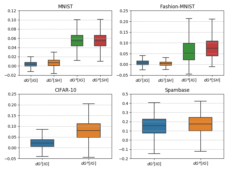
Figure 3: Boxplot of pointwise sparseness-improvements from adversarially trained models (dGa[A](𝐱,ε)𝑑superscript𝐺𝑎delimited-[]𝐴𝐱𝜀dG^{a}[A](\operatorname{{\boldsymbol{x}}},\varepsilon)) and naturally trained models with 1subscript1\ell_{1}-regularization (dGl[A](𝐱,λ)𝑑superscript𝐺𝑙delimited-[]𝐴𝐱𝜆dG^{l}[A](\operatorname{{\boldsymbol{x}}},\lambda)), for attribution methods A{IG,SH}𝐴𝐼𝐺𝑆𝐻A\in\{IG,SH\}.
Refer to caption
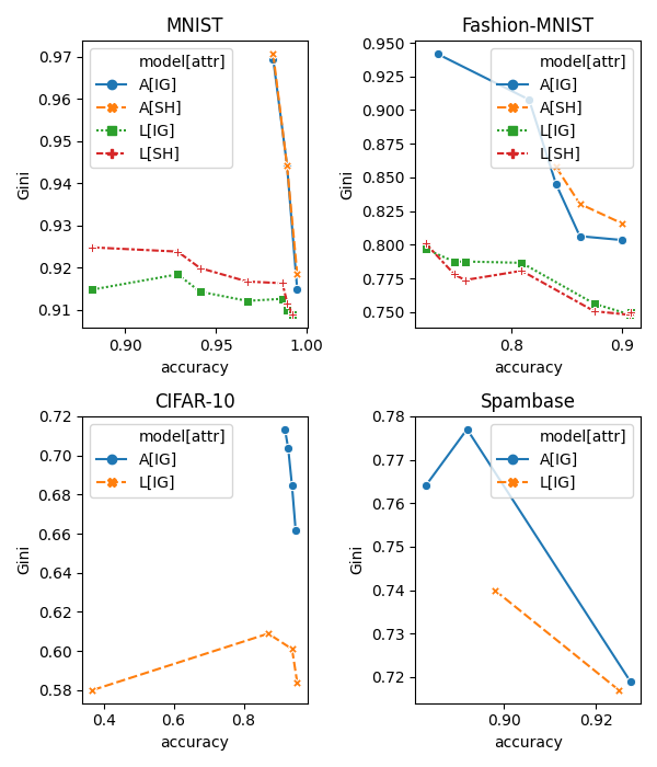
Figure 4: For four benchmark datasets, each line-plot labeled M[A]𝑀delimited-[]𝐴M[A] shows the tradeoff between Accuracy and Attribution Sparseness achievable by various combinations of models M𝑀M and attribution methods A𝐴A. M=A𝑀𝐴M=A denotes (ε)subscript𝜀\ell_{\infty}(\varepsilon)-adversarial training, and the plot shows the accuracy/sparseness for various choices of ε𝜀\varepsilon. M=L𝑀𝐿M=L denotes 1subscript1\ell_{1}-regularized natural training, and the plot shows accuracy/sparseness for various choices of 1subscript1\ell_{1}-regularization parameter λ𝜆\lambda. A=IG𝐴𝐼𝐺A=IG denotes the IG attribution method, whereas A=SH𝐴𝑆𝐻A=SH denotes DeepSHAP. Attribution sparseness is measured by the Average Gini Index over the dataset (Ga[A](ε)superscript𝐺𝑎delimited-[]𝐴𝜀G^{a}[A](\varepsilon) and Gl[A](λ)superscript𝐺𝑙delimited-[]𝐴𝜆G^{l}[A](\lambda), for adversarial training and 1subscript1\ell_{1}-regularized natural training respectively). In all cases, and especially in the image datasets, adversarial training achieves a significantly better accuracy vs attribution sparseness tradeoff.

These results make it clear that for comparable levels of accuracy, the sparseness of attribution vectors from (ε)subscript𝜀\ell_{\infty}(\varepsilon)-adversarially trained models is much better than the sparseness from natural training with 1subscript1\ell_{1}-regularization. The effect is especially pronounced in the two image datasets. The effect is less dramatic in the two tabular datasets, for which we train logistic regression models. Our discussion at the end of Sec. 4 suggests a possible explanation.

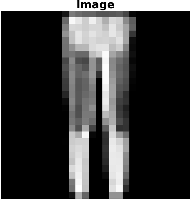
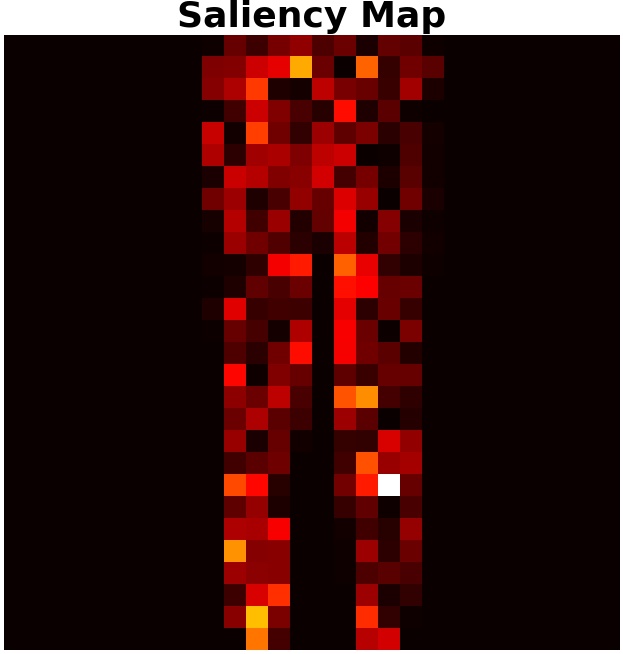
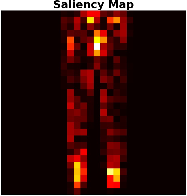
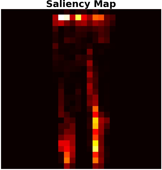
In the Introduction we gave an example of a saliency map (Simonyan et al., 2013; Baehrens et al., 2010) (Fig. 2) to dramatically highlight the sparseness induced by adversarial training. We show several more examples of saliency maps in the supplement (Section J.4).

7 Related Work

In contrast to the growing body of work on defenses against adversarial attacks (Yuan et al., 2017; Madry et al., 2017; Biggio et al., 2013) or explaining adversarial examples (Goodfellow et al., 2014; Tsipras et al., 2018), the focus of our paper is the connection between adversarial robustness and explainability. We view the process of adversarial training as a tool to produce more explainable models. A recent series of papers (Tsipras et al., 2018; Ilyas et al., 2019) essentially argues that adversarial examples exist because standard training produces models are heavily reliant on highly predictive but non-robust features (which is similar to our notion of “weak” features in Sec 3) which are vulnerable to an adversary who can “flip” them and cause performance to degrade. Indeed the authors of (Ilyas et al., 2019) touch upon some connections between explainability and robustness, and conclude, As such, producing human-meaningful explanations that remain faithful to underlying models cannot be pursued independently from the training of the models themselves, by which they are implying that good explainability may require intervening in the model-training procedure itself; this is consistent with our findings. We discuss other related work in the Supplement Section A.

8 Conclusion

We presented theoretical and experimental results that show a strong connection between adversarial robustness (under subscript\ell_{\infty}-bounded perturbations) and two desirable properties of model explanations: conciseness and stability. Specifically, we considered model explanations in the form of feature-attributions based on the Integrated Gradients (IG) and DeepSHAP techniques. For 1-layer models using a popular family of loss functions, we theoretically showed that (ε)subscript𝜀\ell_{\infty}(\varepsilon)-adversarial training tends to produce sparse and stable IG-based attribution vectors. With extensive experiments on benchmark tabular and image datasets, we demonstrated that the “attribution sparsification” effect extends to Deep Neural Networks, when using two popular attribution methods. Intriguingly, especially in DNN models for image classification, the attribution sparseness from natural training with 1subscript1\ell_{1}-regularization is much inferior to that achievable via (ε)subscript𝜀\ell_{\infty}(\varepsilon)-adversarial training. Our theoretical results are a first step in explaining some of these phenomena.

References

  • Abramovich & Grinshtein (2017) Abramovich, F. and Grinshtein, V. High-dimensional classification by sparse logistic regression. June 2017. URL http://arxiv.org/abs/1706.08344.
  • Alvarez-Melis & Jaakkola (2018) Alvarez-Melis, D. and Jaakkola, T. S. On the robustness of interpretability methods. arXiv preprint arXiv:1806. 08049, 2018. URL http://arxiv.org/abs/1806.08049.
  • Ancona et al. (2017) Ancona, M., Ceolini, E., Öztireli, C., and Gross, M. Towards better understanding of gradient-based attribution methods for deep neural networks. November 2017. URL http://arxiv.org/abs/1711.06104.
  • Arya et al. (2019) Arya, V., Bellamy, R. K. E., Chen, P.-Y., Dhurandhar, A., Hind, M., Hoffman, S. C., Houde, S., Vera Liao, Q., Luss, R., Mojsilović, A., Mourad, S., Pedemonte, P., Raghavendra, R., Richards, J., Sattigeri, P., Shanmugam, K., Singh, M., Varshney, K. R., Wei, D., and Zhang, Y. One explanation does not fit all: A toolkit and taxonomy of AI explainability techniques. September 2019. URL http://arxiv.org/abs/1909.03012.
  • Baehrens et al. (2010) Baehrens, D., Schroeter, T., Harmeling, S., Kawanabe, M., Hansen, K., and Müller, K.-R. How to explain individual classification decisions. J. Mach. Learn. Res., 11(Jun):1803–1831, 2010. URL http://www.jmlr.org/papers/volume11/baehrens10a/baehrens10a.pdf.
  • Biggio et al. (2013) Biggio, B., Corona, I., Maiorca, D., Nelson, B., Šrndić, N., Laskov, P., Giacinto, G., and Roli, F. Evasion attacks against machine learning at test time. In Machine Learning and Knowledge Discovery in Databases, pp. 387–402. Springer Berlin Heidelberg, 2013. URL http://dx.doi.org/10.1007/978-3-642-40994-3_25.
  • Dheeru & Karra Taniskidou (2017) Dheeru, D. and Karra Taniskidou, E. UCI machine learning repository, 2017. URL http://archive.ics.uci.edu/ml.
  • Goodfellow et al. (2014) Goodfellow, I. J., Shlens, J., and Szegedy, C. Explaining and harnessing adversarial examples. December 2014. URL http://arxiv.org/abs/1412.6572.
  • Guest & Love (2017) Guest, O. and Love, B. C. What the success of brain imaging implies about the neural code. Elife, 6, January 2017. URL http://dx.doi.org/10.7554/eLife.21397.
  • Hurley & Rickard (2009) Hurley, N. and Rickard, S. Comparing measures of sparsity. IEEE Trans. Inf. Theory, 55(10):4723–4741, October 2009. URL http://dx.doi.org/10.1109/TIT.2009.2027527.
  • Ilyas et al. (2019) Ilyas, A., Santurkar, S., Tsipras, D., Engstrom, L., Tran, B., and Madry, A. Adversarial examples are not bugs, they are features. May 2019. URL http://arxiv.org/abs/1905.02175.
  • Kim et al. (2019) Kim, B., Seo, J., and Jeon, T. Bridging adversarial robustness and gradient interpretability. Safe Machine Learning workshop at ICLR, 2019.
  • LeCun & Cortes (2010) LeCun, Y. and Cortes, C. MNIST handwritten digit database. 2010. URL http://yann.lecun.com/exdb/mnist/.
  • Lundberg & Lee (2017) Lundberg, S. M. and Lee, S.-I. A unified approach to interpreting model predictions. In Advances in Neural Information Processing Systems, pp. 4765–4774, 2017.
  • Madry et al. (2017) Madry, A., Makelov, A., Schmidt, L., Tsipras, D., and Vladu, A. Towards deep learning models resistant to adversarial attacks. June 2017.
  • Molnar (2019) Molnar, C. Interpretable Machine Learning. 2019. https://christophm.github.io/interpretable-ml-book/.
  • Noack et al. (2019) Noack, A., Ahern, I., Dou, D., and Li, B. Does interpretability of neural networks imply adversarial robustness? ArXiv, abs/1912.03430, 2019.
  • Papernot et al. (2015) Papernot, N., McDaniel, P., Jha, S., Fredrikson, M., Berkay Celik, Z., and Swami, A. The limitations of deep learning in adversarial settings. November 2015. URL http://arxiv.org/abs/1511.07528.
  • Ribeiro et al. (2016) Ribeiro, M. T., Singh, S., and Guestrin, C. “why should I trust you?”: Explaining the predictions of any classifier. February 2016. URL http://arxiv.org/abs/1602.04938.
  • Sankaranarayanan et al. (2017) Sankaranarayanan, S., Jain, A., Chellappa, R., and Lim, S. N. Regularizing deep networks using efficient layerwise adversarial training. May 2017. URL http://arxiv.org/abs/1705.07819.
  • Shaham et al. (2015) Shaham, U., Yamada, Y., and Negahban, S. Understanding adversarial training: Increasing local stability of neural nets through robust optimization. November 2015. URL http://arxiv.org/abs/1511.05432.
  • Simonyan et al. (2013) Simonyan, K., Vedaldi, A., and Zisserman, A. Deep inside convolutional networks: Visualising image classification models and saliency maps. CoRR, abs/1312.6034, 2013.
  • Sinha et al. (2018) Sinha, A., Namkoong, H., and Duchi, J. Certifying some distributional robustness with principled adversarial training. February 2018. URL https://openreview.net/pdf?id=Hk6kPgZA-.
  • Sundararajan et al. (2017) Sundararajan, M., Taly, A., and Yan, Q. Axiomatic attribution for deep networks. March 2017.
  • Szegedy et al. (2013) Szegedy, C., Zaremba, W., Sutskever, I., Bruna, J., Erhan, D., Goodfellow, I., and Fergus, R. Intriguing properties of neural networks. December 2013. URL http://arxiv.org/abs/1312.6199.
  • Tan et al. (2013) Tan, M., Tsang, I. W., and Wang, L. Minimax sparse logistic regression for very high-dimensional feature selection. IEEE Trans Neural Netw Learn Syst, 24(10):1609–1622, October 2013. URL http://dx.doi.org/10.1109/TNNLS.2013.2263427.
  • Tan et al. (2014) Tan, M., Tsang, I. W., and Wang, L. Towards ultrahigh dimensional feature selection for big data. J. Mach. Learn. Res., 15(1):1371–1429, 2014. URL http://www.jmlr.org/papers/volume15/tan14a/tan14a.pdf.
  • Tanay & Griffin (2018) Tanay, T. and Griffin, L. D. A new angle on l2 regularization. CoRR, abs/1806.11186, 2018.
  • Tsipras et al. (2018) Tsipras, D., Santurkar, S., Engstrom, L., Turner, A., and Madry, A. Robustness may be at odds with accuracy. May 2018. URL http://arxiv.org/abs/1805.12152.
  • Xiao et al. (2017) Xiao, H., Rasul, K., and Vollgraf, R. Fashion-MNIST: a novel image dataset for benchmarking machine learning algorithms. August 2017. URL http://arxiv.org/abs/1708.07747.
  • Xu et al. (2009) Xu, H., Caramanis, C., and Mannor, S. Robustness and regularization of support vector machines. J. Mach. Learn. Res., 10(Jul):1485–1510, 2009. URL http://www.jmlr.org/papers/volume10/xu09b/xu09b.pdf.
  • Yeh et al. (2019) Yeh, C.-K., Hsieh, C.-Y., Suggala, A., Inouye, D. I., and Ravikumar, P. K. On the (in)fidelity and sensitivity of explanations. In Wallach, H., Larochelle, H., Beygelzimer, A., dAlché Buc, F., Fox, E., and Garnett, R. (eds.), Advances in Neural Information Processing Systems 32, pp.  10967–10978. Curran Associates, Inc., 2019. URL https://arxiv.org/pdf/1901.09392.pdf.
  • Yuan et al. (2017) Yuan, X., He, P., Zhu, Q., and Li, X. Adversarial examples: Attacks and defenses for deep learning. December 2017. URL http://arxiv.org/abs/1712.07107.

Appendix A Additional Related Work

Section 7 discussed some of the work most directly related to this paper. Here we describe some additional related work.

Adversarial Robustness and Interpretability.

Through a very different analysis, (Yeh et al., 2019) show a result closely related to our Theorem 5.1: the show that adversarial training is analogous to making gradient-based explanations more “smooth”, which lowers the sensitivity of gradient explanation. The paper of (Noack et al., 2019) considers a question that is the converse of the one we examine in our paper: They show evidence that models that are forced to have interpretable gradients are more robust to adversarial examples than models trained in a standard manner. Another recent paper (Kim et al., 2019) analyzes the effect of adversarial training on the interpretability of neural network loss gradients.

Relation to work on Regularization Benefits of AML.

There has been prior work on the regularization benefits of adversarial training (Xu et al., 2009; Szegedy et al., 2013; Goodfellow et al., 2014; Shaham et al., 2015; Sankaranarayanan et al., 2017; Tanay & Griffin, 2018), primarily in image-classification applications: when a model is adversarially trained, its classification accuracy on natural (i.e. un-perturbed) test data can improve. All of this prior work has focused on the performance-improvement (on natural test data) aspect of regularization, but none have examined the feature-pruning benefits explicitly. In contrast to this work, our primary interest is in the explainability benefits of adversarial training, and specifically the ability of adversarial training to significantly improve feature-concentration while maintaining (and often improving) performance on natural test data.

Adversarial Training vs Feature-Selection.

Since our results show that adversarial training can effectively shrink the weights of irrelevant or weakly-relevant features (while preserving weights on relevant features), a legitimate counter-proposal might be that one could weed out such features beforehand via a pre-processing step where features with negligible label-correlations can be “removed” from the training process. Besides the fact that this scheme has no guarantees whatsoever with regard to adversarial robustness, there are some practical reasons why correlation-based feature selection is not as effective as adversarial training, in producing pruned models: (a) With adversarial training, one needs to simply try different values of the adversarial strength parameter ε𝜀\varepsilon and find a level where accuracy (or other metric such as AUC-ROC) is not impacted much but model-weights are significantly more concentrated; on the other hand with the correlation-based feature-pruning method, one needs to set up an iterative loop with gradually increasing correlation thresholds, and each time the input pre-processing pipeline needs to be re-executed with a reduced set of features. (b) When there are categorical features with large cardinalities, where just some of the categorical values have negligible feature-correlations, it is not even clear how one can “remove” these specific feature values, since the feature itself must still be used; at the very least it would require a re-encoding of the categorical feature each time a subset of its values is “dropped” (for example if a one-hot encoding or hashing scheme is used). Thus correlation-based feature-pruning is a much more cumbersome and inefficient process compared to adversarial training.

Adversarial Training vs Other Methods to Train Sparse Logistic Regression Models.

(Tan et al., 2013, 2014) propose an approach to train sparse logistic regression models based on a min-max optimization problem that can be solved by the cutting plane algorithm. This requires a specially implemented custom optimization procedure. By contrast, (ε)subscript𝜀\ell_{\infty}(\varepsilon)-adversarial training can be implemented as a simple and efficient “bolt-on” layer on top of existing ML pipelines based on TensorFlow, PyTorch or SciKit-Learn, which makes it highly practical. Another paper (Abramovich & Grinshtein, 2017) proposes a feature selection procedure based on penalized maximum likelihood with a complexity penalty on the model size, but once again this requires special-purpose optimization code.

Appendix B Discussion of Assumptions

B.1 Loss Functions Satisfying Assumption LOSS-CVX

We show here that several popular loss functions satisfy the Assumption LOSS-CVX.

Logistic NLL (Negative Log Likelihood) Loss.
(𝐱,y;𝐰)=ln(σ(y𝐰,𝐱))=ln(1+exp(y𝐰,𝐱))𝐱𝑦𝐰𝜎𝑦𝐰𝐱1𝑦𝐰𝐱\mathcal{L}(\operatorname{{\boldsymbol{x}}},y;\operatorname{{\boldsymbol{w}}})=-\ln(\sigma(y\langle\operatorname{{\boldsymbol{w}}},\,\operatorname{{\boldsymbol{x}}}\rangle))=\ln(1+\exp(-y\langle\operatorname{{\boldsymbol{w}}},\,\operatorname{{\boldsymbol{x}}}\rangle)), which can be written as g(y𝐰,𝐱)𝑔𝑦𝐰𝐱g(-y\langle\operatorname{{\boldsymbol{w}}},\,\operatorname{{\boldsymbol{x}}}\rangle) where g(z)=ln(1+ez)𝑔𝑧1superscript𝑒𝑧g(z)=\ln(1+e^{z}) is a non-decreasing and convex function.

Hinge Loss
(𝐱,y;𝐰)=(1y𝐰,𝐱)+𝐱𝑦𝐰superscript1𝑦𝐰𝐱\mathcal{L}(\operatorname{{\boldsymbol{x}}},y;\operatorname{{\boldsymbol{w}}})=(1-y\langle\operatorname{{\boldsymbol{w}}},\,\operatorname{{\boldsymbol{x}}}\rangle)^{+}
, which can be written as g(y𝐰,𝐱)𝑔𝑦𝐰𝐱g(-y\langle\operatorname{{\boldsymbol{w}}},\,\operatorname{{\boldsymbol{x}}}\rangle) where g(z)=(1+z)+𝑔𝑧superscript1𝑧g(z)=(1+z)^{+} is non-decreasing and convex.

Softplus Hinge Loss.
(𝐱,y;𝐰)=ln(1+exp(1y𝐰,𝐱))𝐱𝑦𝐰11𝑦𝐰𝐱\mathcal{L}(\operatorname{{\boldsymbol{x}}},y;\operatorname{{\boldsymbol{w}}})=\ln(1+\exp(1-y\langle\operatorname{{\boldsymbol{w}}},\,\operatorname{{\boldsymbol{x}}}\rangle))
, which can be written as g(y𝐰,𝐱)𝑔𝑦𝐰𝐱g(-y\langle\operatorname{{\boldsymbol{w}}},\,\operatorname{{\boldsymbol{x}}}\rangle) where g(z)=ln(1+e1+z)𝑔𝑧1superscript𝑒1𝑧g(z)=\ln(1+e^{1+z}), and clearly g𝑔g is non-decreasing. Moreover the first derivative of g𝑔g, g(z)=1/(1+e1z)superscript𝑔𝑧11superscript𝑒1𝑧g^{\prime}(z)=1/(1+e^{-1-z}) is non-decreasing, and therefore g𝑔g is convex.

B.2 Implications of Assumption FEAT-TRANS

Lemma 1.

Given random variables X,Ysuperscript𝑋𝑌X^{\prime},Y where Y{±1}𝑌plus-or-minus1Y\in\{\pm 1\}, if we define X=X[𝔼(X|Y=1)+𝔼(X|Y=1)]/2𝑋superscript𝑋delimited-[]𝔼conditionalsuperscript𝑋𝑌1𝔼conditionalsuperscript𝑋𝑌12X=X^{\prime}-[\mathbb{E}(X^{\prime}|Y=1)+\mathbb{E}(X^{\prime}|Y=-1)]/2, then:

𝔼(X|Y)𝔼conditional𝑋𝑌\displaystyle\mathbb{E}(X|Y) =aYabsent𝑎𝑌\displaystyle=aY (B.23)
𝔼(YX)𝔼𝑌𝑋\displaystyle\mathbb{E}(YX) =𝔼[𝔼(YX|Y)]=𝔼[Y𝔼(X|Y)]=𝔼[Y2a]=aabsent𝔼delimited-[]𝔼conditional𝑌𝑋𝑌𝔼delimited-[]𝑌𝔼conditional𝑋𝑌𝔼delimited-[]superscript𝑌2𝑎𝑎\displaystyle=\mathbb{E}[\mathbb{E}(YX|Y)]=\mathbb{E}[Y\mathbb{E}(X|Y)]=\mathbb{E}[Y^{2}a]=a (B.24)
𝔼(YX|Y)𝔼conditional𝑌𝑋𝑌\displaystyle\mathbb{E}(YX|Y) =Y𝔼[X|Y]=Y2a=a,absent𝑌𝔼delimited-[]conditional𝑋𝑌superscript𝑌2𝑎𝑎\displaystyle=Y\mathbb{E}[X|Y]=Y^{2}a=a, (B.25)

where a=[𝔼(X|Y=1)𝔼(X|Y=1)]/2𝑎delimited-[]𝔼conditionalsuperscript𝑋𝑌1𝔼conditionalsuperscript𝑋𝑌12a=[\mathbb{E}(X^{\prime}|Y=1)-\mathbb{E}(X^{\prime}|Y=-1)]/2.

Proof.

Consider the function f(Y)=𝔼(X|Y)𝑓𝑌𝔼conditionalsuperscript𝑋𝑌f(Y)=\mathbb{E}(X^{\prime}|Y), and let b0:=f(1)assignsubscript𝑏0𝑓1b_{0}:=f(-1) and b1:=f(1)assignsubscript𝑏1𝑓1b_{1}:=f(1). Since there are only two values of Y𝑌Y that are of interest, we can represent f(Y)𝑓𝑌f(Y) by a linear function aY+c𝑎𝑌𝑐aY+c, and it is trivial to verify that a=(b1b0)/2𝑎subscript𝑏1subscript𝑏02a=(b_{1}-b_{0})/2 and c=(b1+b0)/2𝑐subscript𝑏1subscript𝑏02c=(b_{1}+b_{0})/2 are the unique values that are consistent with f(1)=b0𝑓1subscript𝑏0f(-1)=b_{0} and f(1)=b1𝑓1subscript𝑏1f(1)=b_{1}. Thus if X=Xc𝑋superscript𝑋𝑐X=X^{\prime}-c, then 𝔼(X|Y)=aY𝔼conditional𝑋𝑌𝑎𝑌\mathbb{E}(X|Y)=aY, proving (B.23), and the other two properties follow trivially. ∎

Appendix C Expressions for adversarial perturbation and loss-gradient

We show two simple preliminary results for loss functions that satisfy Assumption LOSS-INC: Lemma 2 shows a simple closed form expression for the (ε)subscript𝜀\ell_{\infty}(\varepsilon)-adversarial perturbation, and we use this result to derive an expression for the gradient of the (ε)subscript𝜀\ell_{\infty}(\varepsilon)-adversarial loss (𝐱+δ,y;𝐰)𝐱superscript𝛿𝑦𝐰\mathcal{L}(\operatorname{{\boldsymbol{x}}}+\delta^{*},y;\operatorname{{\boldsymbol{w}}}) with respect to a weight wisubscript𝑤𝑖w_{i} (Lemma 3).

Lemma 2 (Closed form for (ε)subscript𝜀\ell_{\infty}(\varepsilon)-adversarial perturbation).

For a data point (𝐱,y)𝐱𝑦(\operatorname{{\boldsymbol{x}}},y), given model weights 𝐰𝐰\operatorname{{\boldsymbol{w}}}, if the loss function (𝐱,y;𝐰)𝐱𝑦𝐰\mathcal{L}(\operatorname{{\boldsymbol{x}}},y;\operatorname{{\boldsymbol{w}}}) satisfies Assumption LOSS-INC, the (ε)subscript𝜀\ell_{\infty}(\varepsilon)-adversarial perturbation δsuperscript𝛿\delta^{*} is given by:

δ=ysgn(𝐰)ε,superscript𝛿𝑦sgn𝐰𝜀\delta^{*}=-y\operatorname{sgn}(\operatorname{{\boldsymbol{w}}})\varepsilon, (7)

and the corresponding (ε)subscript𝜀\ell_{\infty}(\varepsilon)-adversarial loss is

(𝐱+δ,y;𝐰)=g(ε𝐰1y𝐰,𝐱)𝐱superscript𝛿𝑦𝐰𝑔𝜀subscriptnorm𝐰1𝑦𝐰𝐱\mathcal{L}(\operatorname{{\boldsymbol{x}}}+\delta^{*},y;\;\operatorname{{\boldsymbol{w}}})=g(\varepsilon||\operatorname{{\boldsymbol{w}}}||_{1}-y\langle\operatorname{{\boldsymbol{w}}},\,\operatorname{{\boldsymbol{x}}}\rangle) (8)
Proof.

Assumption LOSS-INC implies that the loss is non-increasing in y𝐰,x𝑦𝐰𝑥y\langle\operatorname{{\boldsymbol{w}}},x\rangle, and therefore the (ε)subscript𝜀\ell_{\infty}(\varepsilon)-perturbation δsuperscript𝛿\delta^{*} of x𝑥x that maximizes the loss would be such that, for each i[d]𝑖delimited-[]𝑑i\in[d], xisubscript𝑥𝑖x_{i} is changed by an amount ε𝜀\varepsilon in the direction of ysgn(wi)𝑦sgnsubscript𝑤𝑖-y\operatorname{sgn}(w_{i}), and the result immediately follows. ∎

Lemma 3 (Gradient of adversarial loss).

For any loss function satisfying Assumption LOSS-INC, for a given data point (𝐱,y)𝐱𝑦(\operatorname{{\boldsymbol{x}}},y), the gradient of the (ε)subscript𝜀\ell_{\infty}(\varepsilon)-adversarial loss is given by:

(𝐱+δ,y;𝐰)wi=g(ε𝐰1y𝐰,𝐱)(yxisgn(wi)ε)𝐱superscript𝛿𝑦𝐰subscript𝑤𝑖superscript𝑔𝜀subscriptnorm𝐰1𝑦𝐰𝐱𝑦subscript𝑥𝑖sgnsubscript𝑤𝑖𝜀\frac{\partial\mathcal{L}(\operatorname{{\boldsymbol{x}}}+\delta^{*},y;\;\operatorname{{\boldsymbol{w}}})}{\partial w_{i}}=-g^{\prime}(\varepsilon||\operatorname{{\boldsymbol{w}}}||_{1}-y\langle\operatorname{{\boldsymbol{w}}},\operatorname{{\boldsymbol{x}}}\rangle)\;(yx_{i}-\operatorname{sgn}(w_{i})\varepsilon) (9)
Proof.

This is straightforward by substituting the expression (7) for δsuperscript𝛿\delta^{*} in g(y𝐰,𝐱+δ)𝑔𝑦𝐰𝐱superscript𝛿g(-y\langle\operatorname{{\boldsymbol{w}}},\operatorname{{\boldsymbol{x}}}+\delta^{*}\rangle), and applying the chain rule. ∎

Appendix D Expectation of SGD Weight Update

The following Lemma will be used to prove Theorem 3.1.

D.1 Upper bound on 𝔼[Zf(Z,V)]𝔼delimited-[]𝑍𝑓𝑍𝑉\mathbb{E}[Zf(Z,V)]

Lemma 4 (Upper Bound on expectation of Zf(Z,V)𝑍𝑓𝑍𝑉Zf(Z,V) when f𝑓f is non-increasing in Z𝑍Z, (ZV)|Yconditionalperpendicular-to𝑍𝑉𝑌(Z\perp V)|Y, and 𝔼(Z|Y)=𝔼(Z)𝔼conditional𝑍𝑌𝔼𝑍\mathbb{E}(Z|Y)=\mathbb{E}(Z)).

For any random variables Z,V𝑍𝑉Z,V, if:

  • f(Z,V)𝑓𝑍𝑉f(Z,V) is non-increasing in Z𝑍Z,

  • Z𝑍Z, V𝑉V are conditionally independent given a third r.v. Y𝑌Y, and

  • 𝔼(Z|Y)=𝔼(Z)𝔼conditional𝑍𝑌𝔼𝑍\mathbb{E}(Z|Y)=\mathbb{E}(Z),

then

𝔼[Zf(Z,V)]𝔼(Z)𝔼[f(Z,V)]𝔼delimited-[]𝑍𝑓𝑍𝑉𝔼𝑍𝔼delimited-[]𝑓𝑍𝑉\mathbb{E}[Zf(Z,V)]\;\leq\;\mathbb{E}(Z)\mathbb{E}[f(Z,V)] (D.26)
Proof.

Let z¯=𝔼(Z)=𝔼(Z|Y)¯𝑧𝔼𝑍𝔼conditional𝑍𝑌\overline{z}=\mathbb{E}(Z)=\mathbb{E}(Z|Y) and note that

𝔼[Zf(Z,V)]𝔼[Z]𝔼[f(Z,V)]𝔼delimited-[]𝑍𝑓𝑍𝑉𝔼delimited-[]𝑍𝔼delimited-[]𝑓𝑍𝑉\displaystyle\mathbb{E}[Zf(Z,V)]-\mathbb{E}[Z]\mathbb{E}[f(Z,V)] =𝔼[Zf(Z,V)]z¯𝔼[f(Z,V)]absent𝔼delimited-[]𝑍𝑓𝑍𝑉¯𝑧𝔼delimited-[]𝑓𝑍𝑉\displaystyle=\mathbb{E}[Zf(Z,V)]-\overline{z}\mathbb{E}[f(Z,V)] (D.27)
=𝔼[(Zz¯)f(Z,V)]absent𝔼delimited-[]𝑍¯𝑧𝑓𝑍𝑉\displaystyle=\mathbb{E}[(Z-\overline{z})f(Z,V)] (D.28)

We want to now argue that 𝔼[(Zz¯)f(z¯,V)]=0𝔼delimited-[]𝑍¯𝑧𝑓¯𝑧𝑉0\mathbb{E}[(Z-\overline{z})f(\overline{z},V)]=0. To see this, apply the Law of Total Expectation by conditioning on Y𝑌Y:

𝔼[(Zz¯)f(z¯,V)]𝔼delimited-[]𝑍¯𝑧𝑓¯𝑧𝑉\displaystyle\mathbb{E}[(Z-\overline{z})f(\overline{z},V)] =𝔼[𝔼[(Zz¯)f(z¯,V)|Y]]absent𝔼delimited-[]𝔼delimited-[]conditional𝑍¯𝑧𝑓¯𝑧𝑉𝑌\displaystyle=\mathbb{E}\Big{[}\mathbb{E}\big{[}(Z-\overline{z})f(\overline{z},V)|Y\big{]}\Big{]}
=𝔼[𝔼[(Zz¯)|Y]𝔼[f(z¯,V)|Y]]absent𝔼delimited-[]𝔼delimited-[]conditional𝑍¯𝑧𝑌𝔼delimited-[]conditional𝑓¯𝑧𝑉𝑌\displaystyle=\mathbb{E}\Big{[}\mathbb{E}\big{[}(Z-\overline{z})|Y\big{]}\mathbb{E}\big{[}f(\overline{z},V)|Y\big{]}\Big{]} (since(ZV)|Y)conditional(sinceperpendicular-to𝑍𝑉𝑌)\displaystyle\text{(since}\;(Z\perp V)|Y\text{)} (D.29)
=0.absent0\displaystyle=0. (since𝔼(Z|Y)=𝔼(Z)=z¯)(since𝔼conditional𝑍𝑌𝔼𝑍¯𝑧)\displaystyle\text{(since}\;\mathbb{E}(Z|Y)=\mathbb{E}(Z)=\overline{z}\text{)} (D.30)

Since 𝔼[(Zz¯)f(z¯,V)]=0𝔼delimited-[]𝑍¯𝑧𝑓¯𝑧𝑉0\mathbb{E}[(Z-\overline{z})f(\overline{z},V)]=0, we can subtract it from the last expectation in (D.28), and by linearity of expectations the RHS of (D.28) can be replaced by

𝔼[(Zz¯)(f(Z,V)f(z¯,V))].𝔼delimited-[]𝑍¯𝑧𝑓𝑍𝑉𝑓¯𝑧𝑉\displaystyle\mathbb{E}\big{[}(Z-\overline{z})(f(Z,V)-f(\overline{z},V))\big{]}. (D.31)

That fact that f(Z,V)𝑓𝑍𝑉f(Z,V) is non-increasing in Z𝑍Z implies that (Zz¯)(f(Z,V)f(z¯,V))0𝑍¯𝑧𝑓𝑍𝑉𝑓¯𝑧𝑉0(Z-\overline{z})(f(Z,V)-f(\overline{z},V))\leq 0 for any value of Z𝑍Z and V𝑉V, with equality when Z=z¯𝑍¯𝑧Z=\overline{z}. Therefore the expectation (D.31) is bounded above by zero, which implies the desired result. ∎

See 3.1

Proof.

Consider the adversarial loss gradient expression (9) from Lemma 3. For the case where wi=0subscript𝑤𝑖0w_{i}=0 for all iS𝑖𝑆i\in S, for any given iS𝑖𝑆i\in S, the negative expectation of the adversarial loss gradient is

Δ¯isubscript¯Δ𝑖\displaystyle\overline{\Delta}_{i} =𝔼[yxig(ε𝐰1y𝐰,𝐱)]absent𝔼delimited-[]𝑦subscript𝑥𝑖superscript𝑔𝜀subscriptnorm𝐰1𝑦𝐰𝐱\displaystyle=\mathbb{E}\big{[}yx_{i}\,g^{\prime}(\varepsilon||\operatorname{{\boldsymbol{w}}}||_{1}-y\langle\operatorname{{\boldsymbol{w}}},\,\operatorname{{\boldsymbol{x}}}\rangle)\big{]}
=𝔼[𝔼[yxig(ε𝐰1y𝐰,𝐱)|y]]absent𝔼delimited-[]𝔼delimited-[]conditional𝑦subscript𝑥𝑖superscript𝑔𝜀subscriptnorm𝐰1𝑦𝐰𝐱𝑦\displaystyle=\mathbb{E}\Big{[}\mathbb{E}\big{[}yx_{i}\,g^{\prime}(\varepsilon||\operatorname{{\boldsymbol{w}}}||_{1}-y\langle\operatorname{{\boldsymbol{w}}},\,\operatorname{{\boldsymbol{x}}}\rangle)\;|y\big{]}\Big{]} (Law of Total Expectation)
=𝔼[y𝔼[xig(ε𝐰1y𝐰,𝐱)|y]],absent𝔼delimited-[]𝑦𝔼delimited-[]conditionalsubscript𝑥𝑖superscript𝑔𝜀subscriptnorm𝐰1𝑦𝐰𝐱𝑦\displaystyle=\mathbb{E}\Big{[}y\,\mathbb{E}\big{[}x_{i}\,g^{\prime}(\varepsilon||\operatorname{{\boldsymbol{w}}}||_{1}-y\langle\operatorname{{\boldsymbol{w}}},\,\operatorname{{\boldsymbol{x}}}\rangle)\;|y\big{]}\Big{]},

and in the last expectation above, we note that since wi=0iSsubscript𝑤𝑖0for-all𝑖𝑆w_{i}=0\;\forall i\in S, the argument of gsuperscript𝑔g^{\prime} does not depend on xisubscript𝑥𝑖x_{i} for any iS𝑖𝑆i\in S, and since the features in S𝑆S are conditionally independent of the rest given the label y𝑦y, xisubscript𝑥𝑖x_{i} is independent of the gsuperscript𝑔g^{\prime} term in the inner conditional expectation. Therefore the inner conditional expectation can be factored as a product of conditional expectations, which gives

Δ¯isubscript¯Δ𝑖\displaystyle\overline{\Delta}_{i} =𝔼[y𝔼(xi|y)𝔼[g(ε𝐰1y𝐰,𝐱)|y]]absent𝔼delimited-[]𝑦𝔼conditionalsubscript𝑥𝑖𝑦𝔼delimited-[]conditionalsuperscript𝑔𝜀subscriptnorm𝐰1𝑦𝐰𝐱𝑦\displaystyle=\mathbb{E}\Big{[}y\mathbb{E}(x_{i}|y)\mathbb{E}\big{[}g^{\prime}(\varepsilon||\operatorname{{\boldsymbol{w}}}||_{1}-y\langle\operatorname{{\boldsymbol{w}}},\,\operatorname{{\boldsymbol{x}}}\rangle)\;|y\big{]}\Big{]}
=𝔼[y2ai𝔼[g(ε𝐰1y𝐰,𝐱)|y]]absent𝔼delimited-[]superscript𝑦2subscript𝑎𝑖𝔼delimited-[]conditionalsuperscript𝑔𝜀subscriptnorm𝐰1𝑦𝐰𝐱𝑦\displaystyle=\mathbb{E}\Big{[}y^{2}a_{i}\mathbb{E}\big{[}g^{\prime}(\varepsilon||\operatorname{{\boldsymbol{w}}}||_{1}-y\langle\operatorname{{\boldsymbol{w}}},\,\operatorname{{\boldsymbol{x}}}\rangle)\;|y\big{]}\Big{]} (Assumption FEAT-TRANS, Eq B.23)
=ai𝔼[𝔼[g(ε𝐰1y𝐰,𝐱)|y]]absentsubscript𝑎𝑖𝔼delimited-[]𝔼delimited-[]conditionalsuperscript𝑔𝜀subscriptnorm𝐰1𝑦𝐰𝐱𝑦\displaystyle=a_{i}\mathbb{E}\Big{[}\mathbb{E}\big{[}g^{\prime}(\varepsilon||\operatorname{{\boldsymbol{w}}}||_{1}-y\langle\operatorname{{\boldsymbol{w}}},\,\operatorname{{\boldsymbol{x}}}\rangle)\;|y\big{]}\Big{]} (since y=±1𝑦plus-or-minus1y=\pm 1)
=aig¯,absentsubscript𝑎𝑖¯superscript𝑔\displaystyle=a_{i}\overline{g^{\prime}}, (D.32)

which establishes the first result.

Now consider the case where wi0subscript𝑤𝑖0w_{i}\neq 0 for at least one iS𝑖𝑆i\in S. Starting with the adversarial loss gradient expression (9) from Lemma 3, for any iS𝑖𝑆i\in S, multiplying throughout by sgn(wi)sgnsubscript𝑤𝑖-\operatorname{sgn}(w_{i}) and taking expectations results in

sgn(wi)Δ¯i=𝔼[[yxisgn(wi)ε]g(εw1y𝐰,𝐱)]sgnsubscript𝑤𝑖subscript¯Δ𝑖𝔼delimited-[]delimited-[]𝑦subscript𝑥𝑖sgnsubscript𝑤𝑖𝜀superscript𝑔𝜀subscriptnorm𝑤1𝑦𝐰𝐱\operatorname{sgn}(w_{i})\overline{\Delta}_{i}=\mathbb{E}\Big{[}\big{[}yx_{i}\operatorname{sgn}(w_{i})-\varepsilon\big{]}\;g^{\prime}(\varepsilon||w||_{1}-y\langle\operatorname{{\boldsymbol{w}}},\,\operatorname{{\boldsymbol{x}}}\rangle)\Big{]} (D.33)

where the expectation is with respect to a random choice of data-point (𝐱,y)𝐱𝑦(\operatorname{{\boldsymbol{x}}},y). The argument of gsuperscript𝑔g^{\prime} can be written as

εw1y𝐰,𝐱=j=1d|wj|(yxjsgn(wj)ε),𝜀subscriptnorm𝑤1𝑦𝐰𝐱superscriptsubscript𝑗1𝑑subscript𝑤𝑗𝑦subscript𝑥𝑗sgnsubscript𝑤𝑗𝜀\varepsilon||w||_{1}-y\langle\operatorname{{\boldsymbol{w}}},\,\operatorname{{\boldsymbol{x}}}\rangle=-\sum_{j=1}^{d}|w_{j}|(yx_{j}\operatorname{sgn}(w_{j})-\varepsilon),

and for j[d]𝑗delimited-[]𝑑j\in[d] if we let Zjsubscript𝑍𝑗Z_{j} denote the random variable corresponding to yxjsgn(wj)ε𝑦subscript𝑥𝑗sgnsubscript𝑤𝑗𝜀yx_{j}\operatorname{sgn}(w_{j})-\varepsilon, then (D.33) can be written as

sgn(wi)Δ¯i=𝔼[Zig(j=1d|wj|Zj)].sgnsubscript𝑤𝑖subscript¯Δ𝑖𝔼delimited-[]subscript𝑍𝑖superscript𝑔superscriptsubscript𝑗1𝑑subscript𝑤𝑗subscript𝑍𝑗\operatorname{sgn}(w_{i})\overline{\Delta}_{i}=\mathbb{E}\left[Z_{i}\;g^{\prime}\left(-\sum_{j=1}^{d}|w_{j}|Z_{j}\right)\right]. (D.34)

Taking the |wi|subscript𝑤𝑖|w_{i}|-weighted average of both sides of (D.34) over iS𝑖𝑆i\in S yields

Δ¯S𝐰=1iS|wi|𝔼[g(j=1d|wj|Zj)iS(|wi|Zi)].subscriptsuperscript¯Δ𝐰𝑆1subscript𝑖𝑆subscript𝑤𝑖𝔼delimited-[]superscript𝑔superscriptsubscript𝑗1𝑑subscript𝑤𝑗subscript𝑍𝑗subscript𝑖𝑆subscript𝑤𝑖subscript𝑍𝑖\overline{\Delta}^{\mathbf{w}}_{S}=\frac{1}{\sum_{i\in S}|w_{i}|}\mathbb{E}\left[g^{\prime}\left(-\sum_{j=1}^{d}|w_{j}|Z_{j}\right)\;\sum_{i\in S}\left(|w_{i}|Z_{i}\right)\right]. (D.35)

If we now define ZS:=iS(|wi|Zi)assignsubscript𝑍𝑆subscript𝑖𝑆subscript𝑤𝑖subscript𝑍𝑖Z_{S}:=\sum_{i\in S}(|w_{i}|Z_{i}), the argument of gsuperscript𝑔g^{\prime} in the expectation above can be written as VSZSsubscript𝑉𝑆subscript𝑍𝑆V_{S}-Z_{S} where VSsubscript𝑉𝑆V_{S} denotes the negative sum of |wj|Zjsubscript𝑤𝑗subscript𝑍𝑗|w_{j}|Z_{j} terms over all jS𝑗𝑆j\not\in S, and thus (D.35) can be written as

Δ¯S𝐰=1iS|wi|𝔼[g(VSZS)ZS].subscriptsuperscript¯Δ𝐰𝑆1subscript𝑖𝑆subscript𝑤𝑖𝔼delimited-[]superscript𝑔subscript𝑉𝑆subscript𝑍𝑆subscript𝑍𝑆\overline{\Delta}^{\mathbf{w}}_{S}=\frac{1}{\sum_{i\in S}|w_{i}|}\mathbb{E}\left[g^{\prime}\left(V_{S}-Z_{S}\right)Z_{S}\right]. (D.36)

Note that ZSsubscript𝑍𝑆Z_{S} is a function of Y𝑌Y and the features in S𝑆S, and VSsubscript𝑉𝑆V_{S} is a function of Y𝑌Y and the features in the complement of S𝑆S. Since the features in S𝑆S are conditionally independent of the rest given the label Y𝑌Y (this is a condition of the Theorem), it follows that (VSZS)|Yconditionalperpendicular-tosubscript𝑉𝑆subscript𝑍𝑆𝑌(V_{S}\perp Z_{S})|Y. Since by Assumption LOSS-CVX, gsuperscript𝑔g^{\prime} is a non-decreasing function, g(VSZS)superscript𝑔subscript𝑉𝑆subscript𝑍𝑆g^{\prime}(V_{S}-Z_{S}) is non-increasing in ZSsubscript𝑍𝑆Z_{S}. Thus all three conditions of Lemma 4 are satisfied, with the random variables Z,V,Y𝑍𝑉𝑌Z,V,Y and function f𝑓f in the Lemma corresponding to random variables ZS,VS,Ysubscript𝑍𝑆subscript𝑉𝑆𝑌Z_{S},V_{S},Y and function gsuperscript𝑔g^{\prime} respectively in the present Theorem. It then follows from Lemma 4 that

Δ¯S𝐰1iS|wi|E(ZS)g¯.subscriptsuperscript¯Δ𝐰𝑆1subscript𝑖𝑆subscript𝑤𝑖𝐸subscript𝑍𝑆¯superscript𝑔\overline{\Delta}^{\mathbf{w}}_{S}\leq\frac{1}{\sum_{i\in S}|w_{i}|}E(Z_{S})\overline{g^{\prime}}. (D.37)

The definition of ZSsubscript𝑍𝑆Z_{S}, and the fact that 𝔼(Zi)=sgn(wi)𝔼(yxi)ε𝔼subscript𝑍𝑖sgnsubscript𝑤𝑖𝔼𝑦subscript𝑥𝑖𝜀\mathbb{E}(Z_{i})=\operatorname{sgn}(w_{i})\mathbb{E}(yx_{i})-\varepsilon = aisgn(wi)εsubscript𝑎𝑖sgnsubscript𝑤𝑖𝜀a_{i}\operatorname{sgn}(w_{i})-\varepsilon (property (4)), imply

𝔼(ZS)=iS[|wi|sgn(wi)ai]εiS|wi|,𝔼subscript𝑍𝑆subscript𝑖𝑆delimited-[]subscript𝑤𝑖sgnsubscript𝑤𝑖subscript𝑎𝑖𝜀subscript𝑖𝑆subscript𝑤𝑖\mathbb{E}(Z_{S})=\sum_{i\in S}\left[|w_{i}|\operatorname{sgn}(w_{i})a_{i}\right]-\varepsilon\sum_{i\in S}|w_{i}|,

and the definition of aS𝐰subscriptsuperscript𝑎𝐰𝑆a^{\mathbf{w}}_{S} allows us to simplify (D.37) to

Δ¯S𝐰g¯(aS𝐰ε),subscriptsuperscript¯Δ𝐰𝑆¯superscript𝑔subscriptsuperscript𝑎𝐰𝑆𝜀\overline{\Delta}^{\mathbf{w}}_{S}\leq\overline{g^{\prime}}(a^{\mathbf{w}}_{S}-\varepsilon),\\

which establishes the upper bound (12).

To analyze the limiting case where wi0subscript𝑤𝑖0w_{i}\rightarrow 0 for all iS𝑖𝑆i\in S, write Eq. (D.36) as follows:

Δ¯S𝐰=𝔼[g(VSZS)ZSiS|wi|].subscriptsuperscript¯Δ𝐰𝑆𝔼delimited-[]superscript𝑔subscript𝑉𝑆subscript𝑍𝑆subscript𝑍𝑆subscript𝑖𝑆subscript𝑤𝑖\overline{\Delta}^{\mathbf{w}}_{S}=\mathbb{E}\left[g^{\prime}\left(V_{S}-Z_{S}\right)\frac{Z_{S}}{\sum_{i\in S}|w_{i}|}\right]. (D.38)

If we let |wi|0subscript𝑤𝑖0|w_{i}|\rightarrow 0 for all iS𝑖𝑆i\in S, the ZSsubscript𝑍𝑆Z_{S} in the argument of gsuperscript𝑔g^{\prime} can be set to 0, and we can write the RHS of (D.38) as

Δ¯S𝐰=𝔼[g(VS)ZSiS|wi|]=𝔼[𝔼[g(VS)ZSiS|wi||Y]],subscriptsuperscript¯Δ𝐰𝑆𝔼delimited-[]superscript𝑔subscript𝑉𝑆subscript𝑍𝑆subscript𝑖𝑆subscript𝑤𝑖𝔼delimited-[]𝔼delimited-[]conditionalsuperscript𝑔subscript𝑉𝑆subscript𝑍𝑆subscript𝑖𝑆subscript𝑤𝑖𝑌\overline{\Delta}^{\mathbf{w}}_{S}=\mathbb{E}\left[g^{\prime}(V_{S})\frac{Z_{S}}{\sum_{i\in S}|w_{i}|}\right]=\mathbb{E}\bigg{[}\mathbb{E}\left[g^{\prime}(V_{S})\frac{Z_{S}}{\sum_{i\in S}|w_{i}|}\;\>\Big{|}\>Y\right]\bigg{]}, (D.39)

where the inner conditional expectation can be factored as a product of conditional expectations since (ZSVS|Y)perpendicular-tosubscript𝑍𝑆conditionalsubscript𝑉𝑆𝑌(Z_{S}\perp V_{S}|Y):

Δ¯S𝐰=𝔼[𝔼[g(VS)|Y]𝔼[ZSiS|wi||Y]].subscriptsuperscript¯Δ𝐰𝑆𝔼delimited-[]𝔼delimited-[]conditionalsuperscript𝑔subscript𝑉𝑆𝑌𝔼delimited-[]conditionalsubscript𝑍𝑆subscript𝑖𝑆subscript𝑤𝑖𝑌\overline{\Delta}^{\mathbf{w}}_{S}=\mathbb{E}\bigg{[}\mathbb{E}\left[g^{\prime}(V_{S})\>\Big{|}\>Y\right]\mathbb{E}\left[\frac{Z_{S}}{\sum_{i\in S}|w_{i}|}\;\>\Big{|}\>Y\right]\bigg{]}. (D.40)

Now notice that

𝔼(ZS|Y)=𝔼[iS(|wi|Zi)|Y]=iS|wi|𝔼[sgn(wi)Yxiε|Y].𝔼conditionalsubscript𝑍𝑆𝑌𝔼delimited-[]conditionalsubscript𝑖𝑆subscript𝑤𝑖subscript𝑍𝑖𝑌subscript𝑖𝑆subscript𝑤𝑖𝔼delimited-[]sgnsubscript𝑤𝑖𝑌subscript𝑥𝑖conditional𝜀𝑌\mathbb{E}(Z_{S}|Y)=\mathbb{E}\left[\sum_{i\in S}(|w_{i}|Z_{i})\>\Big{|}\>Y\right]=\sum_{i\in S}|w_{i}|\;\mathbb{E}\left[\operatorname{sgn}(w_{i})Yx_{i}-\varepsilon\;|\;Y\right]. (D.41)

From Property (5) of datasets satisfying Assumption FEAT-TRANS, 𝔼[Yxi|Y]=𝔼(Yxi)=ai𝔼delimited-[]conditional𝑌subscript𝑥𝑖𝑌𝔼𝑌subscript𝑥𝑖subscript𝑎𝑖\mathbb{E}[Yx_{i}|Y]=\mathbb{E}(Yx_{i})=a_{i}, and so the second inner expectation in (D.40) simplifies to a constant:

𝔼[ZSiS|wi||Y]=iS[|wi|sgn(wi)ai]iS|wi|ε=aS𝐰ε.𝔼delimited-[]conditionalsubscript𝑍𝑆subscript𝑖𝑆subscript𝑤𝑖𝑌subscript𝑖𝑆delimited-[]subscript𝑤𝑖sgnsubscript𝑤𝑖subscript𝑎𝑖subscript𝑖𝑆subscript𝑤𝑖𝜀subscriptsuperscript𝑎𝐰𝑆𝜀\mathbb{E}\left[\frac{Z_{S}}{\sum_{i\in S}|w_{i}|}\;\>\Big{|}\>Y\right]=\frac{\sum_{i\in S}\left[|w_{i}|\operatorname{sgn}(w_{i})a_{i}\right]}{\sum_{i\in S}|w_{i}|}-\varepsilon=a^{\mathbf{w}}_{S}-\varepsilon. (D.42)

Eq. (D.40) can therefore be simplified to

Δ¯S𝐰=𝔼[𝔼[g(VS)|Y]](aS𝐰ε)=g¯(aS𝐰ε),subscriptsuperscript¯Δ𝐰𝑆𝔼delimited-[]𝔼delimited-[]conditionalsuperscript𝑔subscript𝑉𝑆𝑌subscriptsuperscript𝑎𝐰𝑆𝜀¯superscript𝑔subscriptsuperscript𝑎𝐰𝑆𝜀\overline{\Delta}^{\mathbf{w}}_{S}=\mathbb{E}\bigg{[}\mathbb{E}\left[g^{\prime}(V_{S})\>\Big{|}\>Y\right]\bigg{]}\left(a^{\mathbf{w}}_{S}-\varepsilon\right)=\overline{g^{\prime}}(a^{\mathbf{w}}_{S}-\varepsilon), (D.43)

which shows the final statement of the Theorem, namely, that if wi0subscript𝑤𝑖0w_{i}\rightarrow 0 for all iS𝑖𝑆i\in S, then (12) holds with equality. ∎

D.2 Implications of Theorem 3.1

Keeping in mind the interpretations of the 𝐰𝐰\mathbf{w}-weighted average quantities aS𝐰subscriptsuperscript𝑎𝐰𝑆a^{\mathbf{w}}_{S} and Δ¯S𝐰subscriptsuperscript¯Δ𝐰𝑆\overline{\Delta}^{\mathbf{w}}_{S} described in the paragraph after the statement of Theorem 3.1, we can state the following implications of this result:

If all weights of S𝑆S are zero, then they grow in the correct direction. When wi=0subscript𝑤𝑖0w_{i}=0 for all iS𝑖𝑆i\in S (recall that S𝑆S is a subset of features, conditionally independent of the rest given the label y𝑦y), the expected SGD update Δ¯isubscript¯Δ𝑖\overline{\Delta}_{i} for each iS𝑖𝑆i\in S is proportional to the directed strength aisubscript𝑎𝑖a_{i} of feature xisubscript𝑥𝑖x_{i}, and if g¯0¯superscript𝑔0\overline{g^{\prime}}\neq 0, this means that on average the SGD update causes the weight wisubscript𝑤𝑖w_{i} to grow from zero in the correct direction. This is what one would expect from an SGD training procedure.

If the weights of S𝑆S are mis-aligned weights on average, then they shrink at a rate proportional to ε+|aS𝐰|𝜀subscriptsuperscript𝑎𝐰𝑆\varepsilon+|a^{\mathbf{w}}_{S}|. Suppose for at least one iS𝑖𝑆i\in S, wi0subscript𝑤𝑖0w_{i}\neq 0, and aS𝐰<0subscriptsuperscript𝑎𝐰𝑆0a^{\mathbf{w}}_{S}<0, i.e. the weights of the features in S𝑆S are mis-aligned on average. In this case by (12), Δ¯S𝐰<0subscriptsuperscript¯Δ𝐰𝑆0\overline{\Delta}^{\mathbf{w}}_{S}<0, i.e. the weights of the features in S𝑆S, in aggregate (i.e. in the |wi|subscript𝑤𝑖|w_{i}|-weighted sense) shrink toward zero in expectation. The aggregate rate of this shrinkage is proportional to ε+|aS𝐰|𝜀subscriptsuperscript𝑎𝐰𝑆\varepsilon+|a^{\mathbf{w}}_{S}|. In other words, all other factors remaining the same, adversarial training (i.e. with ε>0𝜀0\varepsilon>0) shrinks mis-aligned faster than natural training (i.e. with ε=0𝜀0\varepsilon=0).

If the weights of S𝑆S are aligned on average, and ε>|aS𝐰|𝜀subscriptsuperscript𝑎𝐰𝑆\varepsilon>|a^{\mathbf{w}}_{S}| then they shrink at a rate proportional to ε|aS𝐰|𝜀subscriptsuperscript𝑎𝐰𝑆\varepsilon-|a^{\mathbf{w}}_{S}|. Suppose that wi0subscript𝑤𝑖0w_{i}\neq 0 for at least one iS𝑖𝑆i\in S, and the weights of S𝑆S are aligned on average, i.e. aS𝐰>0subscriptsuperscript𝑎𝐰𝑆0a^{\mathbf{w}}_{S}>0. Even in this case, the weights of S𝑆S shrink on average, provided the alignment strength aS𝐰subscriptsuperscript𝑎𝐰𝑆a^{\mathbf{w}}_{S} is dominated by the adversarial ε𝜀\varepsilon; the rate of shrinkage is proportional to ε|aS𝐰|𝜀subscriptsuperscript𝑎𝐰𝑆\varepsilon-|a^{\mathbf{w}}_{S}|, by Eq. (12). Thus adversarial training with a sufficiently large ε𝜀\varepsilon that dominates the average strength of the features in S𝑆S, will cause the weights of these features to shrink on average. This observation is key to explaining the “feature-pruning” behavior of adversarial training: “weak” features (relative to ε𝜀\varepsilon) are weeded out by the SGD updates.

If the weights of S𝑆S are aligned, ε<|aS𝐰|𝜀subscriptsuperscript𝑎𝐰𝑆\varepsilon<|a^{\mathbf{w}}_{S}|, then the weights of S𝑆S expand up to a certain point. Consider the case where at least one of the S𝑆S weights is non-zero, and the adversarial ε𝜀\varepsilon does not dominate the average strength aS𝐰subscriptsuperscript𝑎𝐰𝑆a^{\mathbf{w}}_{S}. Again from Eq. (12), if aS𝐰>0subscriptsuperscript𝑎𝐰𝑆0a^{\mathbf{w}}_{S}>0 and ε<|aS𝐰|𝜀subscriptsuperscript𝑎𝐰𝑆\varepsilon<|a^{\mathbf{w}}_{S}|, then the upper bound (12) on Δ¯S𝐰subscriptsuperscript¯Δ𝐰𝑆\overline{\Delta}^{\mathbf{w}}_{S} is non-negative. Since the Theorem states that equality holds in the limit as wi0subscript𝑤𝑖0w_{i}\rightarrow 0 for all iS𝑖𝑆i\in S, this means if all |wi|subscript𝑤𝑖|w_{i}| for iS𝑖𝑆i\in S are sufficiently small, the expected SGD update Δ¯S𝐰subscriptsuperscript¯Δ𝐰𝑆\overline{\Delta}^{\mathbf{w}}_{S} is non-negative, i.e., the S𝑆S weights expand on average. In other words, the weights of a conditionally independent feature-subset S𝑆S, if they are aligned on average, then their aggregate weights expand on average up to a certain point, if ε𝜀\varepsilon does not dominate their strength.

Note that Assumption LOSS-CVX implies that g¯0¯superscript𝑔0\overline{g^{\prime}}\geq 0, and when the model 𝐰𝐰\operatorname{{\boldsymbol{w}}} is “far” from the optimum, the values of y𝐰,𝐱𝑦𝐰𝐱-y\langle\operatorname{{\boldsymbol{w}}},\,\operatorname{{\boldsymbol{x}}}\rangle will tend to be large, and since gsuperscript𝑔g^{\prime} is a non-decreasing function (Assumption LOSS-CVX), g¯¯superscript𝑔\overline{g^{\prime}} will be large as well. So we can interpret g¯¯superscript𝑔\overline{g^{\prime}} as being a proxy for “average model error”. Thus during the initial iterations of SGD, this quantity will tend to be large and positive, and shrinks toward zero as the model approaches optimality. Since g¯¯superscript𝑔\overline{g^{\prime}} appears as a factor in (11) and (12), we can conclude that the above effects will be more pronounced in the initial stages of SGD and less so in the later stages. The experimental results described in Section 6 are consistent with several of the above effects.

Appendix E Generalization of Theorem 3.1 for the multi-class setting

E.1 Setting and Assumptions

Let there be k3𝑘3k\geq 3 classes. For a given data point 𝐱d𝐱superscript𝑑\mathbf{x}\in\mathbb{R}^{d}, its true label, i[k]𝑖delimited-[]𝑘i\in[k], is represented by a vector 𝐲=[11i-1111k-i]𝐲delimited-[]subscript11i-11subscript11k-i\mathbf{y}=[\underbrace{-1\cdots-1}_{\text{i-1}}1\underbrace{-1\cdots-1}_{\text{k-i}}]. We assume that the input (𝐱,𝐲)𝐱𝐲(\mathbf{x},\mathbf{y}) is drawn from the distribution 𝒟𝒟\mathcal{D}. For this multi-class classification problem, we assume the usage of the standard one-vs-all classifiers, i.e., there are k𝑘k different classifiers with the i𝑖i-th classifier (ideally) predicting +11+1 iff the true label of 𝐱𝐱\mathbf{x} is i𝑖i, else it predicts 11-1. Let 𝐰𝐰\mathbf{w} represent the k×d𝑘𝑑k\times d weight matrix where 𝐰𝐢subscript𝐰𝐢\mathbf{w_{i}} represents the 1×d1𝑑1\times d weight vector for the i𝑖i-th classifier. wijsubscript𝑤𝑖𝑗w_{ij} represents the j𝑗j-th entry of 𝐰𝐢subscript𝐰𝐢\mathbf{w_{i}}. Let yisubscript𝑦𝑖y_{i} represent the i𝑖i-th entry of 𝐲𝐲\mathbf{y}.

The assumptions presented in the main paper (Sec. 2) are slightly tweaked as follows and hold true for each of the k𝑘k one-vs-all classifiers:

Assumption LOSS-INC: The loss function for each of the one-vs-all classifier is of the form (𝐱,yi;𝐰𝐢)=g(yi𝐰𝐢,𝐱)𝐱subscript𝑦𝑖subscript𝐰𝐢𝑔subscript𝑦𝑖subscript𝐰𝐢𝐱\mathcal{L}(\mathbf{x},y_{i};\mathbf{w_{i}})=g(-y_{i}\langle\mathbf{w_{i}},\mathbf{x}\rangle) where g𝑔g is a non-decreasing function.

Assumption LOSS-CVX: The loss function for each of the one-vs-all classifier is of the form (𝐱,yi;𝐰𝐢)=g(yi𝐰𝐢,𝐱)𝐱subscript𝑦𝑖subscript𝐰𝐢𝑔subscript𝑦𝑖subscript𝐰𝐢𝐱\mathcal{L}(\mathbf{x},y_{i};\mathbf{w_{i}})=g(-y_{i}\langle\mathbf{w_{i}},\mathbf{x}\rangle) where g𝑔g is non-decreasing, almost-everywhere differentiable and convex.

Assumption FEAT-INDEP: The features 𝐱𝐱\mathbf{x} are conditionally independent given the label yisubscript𝑦𝑖y_{i} for the i𝑖i-th one-vs-all classifier, i.e., for any two distinct induces s,t𝑠𝑡s,t, xssubscript𝑥𝑠x_{s} is independent of xtsubscript𝑥𝑡x_{t} given yisubscript𝑦𝑖y_{i}, or more compactly, (xsxt)|yiconditionalperpendicular-tosubscript𝑥𝑠subscript𝑥𝑡subscript𝑦𝑖(x_{s}\perp x_{t})\thinspace|\thinspace y_{i}.

Assumption FEAT-EXP: For each feature xj,j[d]subscript𝑥𝑗𝑗delimited-[]𝑑x_{j},j\in[d] and the i𝑖i-th one-vs-all classifier 𝔼(xj|yi)=aij.yiformulae-sequence𝔼conditionalsubscript𝑥𝑗subscript𝑦𝑖subscript𝑎𝑖𝑗subscript𝑦𝑖\mathbb{E}(x_{j}|y_{i})=a_{ij}.y_{i} for some constant aijsubscript𝑎𝑖𝑗a_{ij}.

Additionally, we introduce a new assumption on the distribution 𝒟𝒟\mathcal{D} as follows.

Assumption DIST-EXPC: The input distribution 𝒟𝒟\mathcal{D} satisfies the following expectation for a function hi,i[k]subscript𝑖𝑖delimited-[]𝑘h_{i},i\in[k] (defined by Eqs. (E.47),(E.48), (E.49)) and constant gsuperscript𝑔g^{*} (defined by Eq. (E.46))

𝔼[hi(sgn(wij)yi,𝐱,𝐰𝐢,ϵ)]=0𝔼delimited-[]subscript𝑖sgnsubscript𝑤𝑖𝑗subscript𝑦𝑖𝐱subscript𝐰𝐢italic-ϵ0\displaystyle\mathbb{E}\Big{[}h_{i}(\text{sgn}(w_{ij})y_{i},\mathbf{x},\mathbf{w_{i}},\epsilon)\Big{]}=0 (E.44)
Pr𝒟[ϵ<xj<ϵ+ρ]=0,ρ is a small constant𝑃subscript𝑟𝒟delimited-[]italic-ϵsubscript𝑥𝑗italic-ϵ𝜌0𝜌 is a small constant\displaystyle Pr_{\mathcal{D}}[\epsilon<x_{j}<\epsilon+\rho]=0,\hskip 8.5359pt\rho\text{ is a small constant} (E.45)
xjϵ+ρ(xjϵ)gi(xj+ϵ)g(yi𝐰𝐢,𝐱+δ)subscript𝑥𝑗italic-ϵ𝜌subscript𝑥𝑗italic-ϵsubscriptsuperscript𝑔𝑖subscript𝑥𝑗italic-ϵsuperscript𝑔subscript𝑦𝑖subscript𝐰𝐢𝐱superscript𝛿\displaystyle x_{j}\geq\epsilon+\rho\implies(x_{j}-\epsilon)g^{*}_{i}\geq(x_{j}+\epsilon)g^{\prime}(-y_{i}\langle\mathbf{w_{i}},\mathbf{x}+\delta^{*}\rangle) (E.46)
 If yisgn(wij)=1, then If subscript𝑦𝑖sgnsubscript𝑤𝑖𝑗1 then\displaystyle\text{ If }y_{i}\text{sgn}(w_{ij})=-1,\text{ then}
h(sgn(wij)yi,𝐱,𝐰𝐢,ϵ)(xj+ϵ)gi(xjϵ)g(yi𝐰𝐢,𝐱+δ)sgnsubscript𝑤𝑖𝑗subscript𝑦𝑖𝐱subscript𝐰𝐢italic-ϵsubscript𝑥𝑗italic-ϵsubscriptsuperscript𝑔𝑖subscript𝑥𝑗italic-ϵsuperscript𝑔subscript𝑦𝑖subscript𝐰𝐢𝐱superscript𝛿\displaystyle h(\text{sgn}(w_{ij})y_{i},\mathbf{x},\mathbf{w_{i}},\epsilon)\geq(x_{j}+\epsilon)g^{*}_{i}-(x_{j}-\epsilon)g^{\prime}(-y_{i}\langle\mathbf{w_{i}},\mathbf{x}+\delta^{*}\rangle) (E.47)
 If yisgn(wij)=1xj>ϵ, thenformulae-sequence If subscript𝑦𝑖sgnsubscript𝑤𝑖𝑗1subscript𝑥𝑗italic-ϵ then\displaystyle\text{ If }y_{i}\text{sgn}(w_{ij})=1\wedge x_{j}>\epsilon,\text{ then}
((xjϵ)gi(xj+ϵ)g(yi𝐰𝐢,𝐱+δ))h(sgn(wij)yi,𝐱,𝐰𝐢,ϵ)0subscript𝑥𝑗italic-ϵsubscriptsuperscript𝑔𝑖subscript𝑥𝑗italic-ϵsuperscript𝑔subscript𝑦𝑖subscript𝐰𝐢𝐱superscript𝛿sgnsubscript𝑤𝑖𝑗subscript𝑦𝑖𝐱subscript𝐰𝐢italic-ϵ0\displaystyle-\Big{(}(x_{j}-\epsilon)g^{*}_{i}-(x_{j}+\epsilon)g^{\prime}(-y_{i}\langle\mathbf{w_{i}},\mathbf{x}+\delta^{*}\rangle)\Big{)}\leq h(\text{sgn}(w_{ij})y_{i},\mathbf{x},\mathbf{w_{i}},\epsilon)\leq 0 (E.48)
 If yisgn(wij)=1xjϵ, thenformulae-sequence If subscript𝑦𝑖sgnsubscript𝑤𝑖𝑗1subscript𝑥𝑗italic-ϵ then\displaystyle\text{ If }y_{i}\text{sgn}(w_{ij})=1\wedge x_{j}\leq\epsilon,\text{ then}
h(sgn(wij)yi,𝐱,𝐰𝐢,ϵ)(xj+ϵ)g(yi𝐰𝐢,𝐱+δ)(xjϵ)gisgnsubscript𝑤𝑖𝑗subscript𝑦𝑖𝐱subscript𝐰𝐢italic-ϵsubscript𝑥𝑗italic-ϵsuperscript𝑔subscript𝑦𝑖subscript𝐰𝐢𝐱superscript𝛿subscript𝑥𝑗italic-ϵsubscriptsuperscript𝑔𝑖\displaystyle h(\text{sgn}(w_{ij})y_{i},\mathbf{x},\mathbf{w_{i}},\epsilon)\geq(x_{j}+\epsilon)g^{\prime}(-y_{i}\langle\mathbf{w_{i}},\mathbf{x}+\delta^{*}\rangle)-(x_{j}-\epsilon)g^{*}_{i} (E.49)

This assumption is not as restrictive as it may appear. Eq. E.45 can be satisfied naturally for discrete domains. For example, for images xj{0,1,2,,254,255}subscript𝑥𝑗012254255x_{j}\in\{0,1,2,\cdots,254,255\}; thus ρ(0,1)𝜌01\rho\in(0,1). For continuous domains, ρ𝜌\rho can be set to a small value and the values of xjsubscript𝑥𝑗x_{j} can be appropriately rounded in the input dataset.
For the rest of the discussion let us consider the case where g(z)=csuperscript𝑔𝑧𝑐g^{\prime}(z)=c (for example for hinge loss function c=1𝑐1c=1 for z>1𝑧1z>-1) and xj[0,1]subscript𝑥𝑗01x_{j}\in[0,1]. Now consider,

g=(1+ϵ)c/ρ,ρ=0.01formulae-sequencesuperscript𝑔1italic-ϵ𝑐𝜌𝜌0.01\displaystyle g^{*}=(1+\epsilon)c/\rho,\hskip 2.84544pt\rho=0.01
f1(x):=((x+ϵ)g(xϵ)c)assignsubscript𝑓1𝑥𝑥italic-ϵsuperscript𝑔𝑥italic-ϵ𝑐\displaystyle f_{1}(x):=((x+\epsilon)g^{*}-(x-\epsilon)c)
f2(x):=((x+ϵ)c(xϵ)g)assignsubscript𝑓2𝑥𝑥italic-ϵ𝑐𝑥italic-ϵsuperscript𝑔\displaystyle f_{2}(x):=((x+\epsilon)c-(x-\epsilon)g^{*})
hi(sgn(wij)yi,𝐱,𝐰𝐢,ϵ)={f1(xj)if sgn(wij)yi=+1f2(xj)otherwisesubscript𝑖sgnsubscript𝑤𝑖𝑗subscript𝑦𝑖𝐱subscript𝐰𝐢italic-ϵcasessubscript𝑓1subscript𝑥𝑗if sgnsubscript𝑤𝑖𝑗subscript𝑦𝑖1otherwisesubscript𝑓2subscript𝑥𝑗otherwiseotherwise\displaystyle h_{i}(\text{sgn}(w_{ij})y_{i},\mathbf{x},\mathbf{w_{i}},\epsilon)=\begin{cases}f_{1}(x_{j})\hskip 11.38092pt\mbox{if }\text{sgn}(w_{ij})y_{i}=+1\\ f_{2}(x_{j})\hskip 11.38092pt\mbox{otherwise}\end{cases}
𝔼[hi(sgn(wij)yi,𝐱,𝐰𝐢,ϵ)]=01Pr[xj|yisgn(wij)=1]f1(xj)𝑑x+𝔼delimited-[]subscript𝑖sgnsubscript𝑤𝑖𝑗subscript𝑦𝑖𝐱subscript𝐰𝐢italic-ϵlimit-fromsuperscriptsubscript01𝑃𝑟delimited-[]conditionalsubscript𝑥𝑗subscript𝑦𝑖sgnsubscript𝑤𝑖𝑗1subscript𝑓1subscript𝑥𝑗differential-d𝑥\displaystyle\mathbb{E}[h_{i}(\text{sgn}(w_{ij})y_{i},\mathbf{x},\mathbf{w_{i}},\epsilon)]=\int_{0}^{1}Pr[x_{j}|y_{i}\text{sgn}(w_{ij})=-1]\cdot f_{1}(x_{j})dx+
ϵ1Pr[xj|yisgn(wij)=+1]f2(x)𝑑x+0ϵPr[xj|yisgn(wij)=+1]f2(x)𝑑xsuperscriptsubscriptitalic-ϵ1𝑃𝑟delimited-[]conditionalsubscript𝑥𝑗subscript𝑦𝑖sgnsubscript𝑤𝑖𝑗1subscript𝑓2𝑥differential-d𝑥superscriptsubscript0italic-ϵ𝑃𝑟delimited-[]conditionalsubscript𝑥𝑗subscript𝑦𝑖sgnsubscript𝑤𝑖𝑗1subscript𝑓2𝑥differential-d𝑥\displaystyle\hskip 28.45274pt\int_{\epsilon}^{1}Pr[x_{j}|y_{i}\text{sgn}(w_{ij})=+1]\cdot f_{2}(x)dx+\int_{0}^{\epsilon}Pr[x_{j}|y_{i}\text{sgn}(w_{ij})=+1]\cdot f_{2}(x)dx

We observe that f1(x)subscript𝑓1𝑥f_{1}(x) is increasing in x[0,1]𝑥01x\in[0,1], and xϵ+δf2(x)0𝑥italic-ϵ𝛿subscript𝑓2𝑥0x\geq\epsilon+\delta\implies f_{2}(x)\leq 0 and f2(x)subscript𝑓2𝑥f_{2}(x) is decreasing in x[ϵ+δ,1]𝑥italic-ϵ𝛿1x\in[\epsilon+\delta,1]. Thus intuitively for 𝔼(hi)𝔼subscript𝑖\mathbb{E}(h_{i}) to be zero, Pr[xj|sgn(wij)yi=1]𝑃𝑟delimited-[]conditionalsubscript𝑥𝑗sgnsubscript𝑤𝑖𝑗subscript𝑦𝑖1Pr[x_{j}|\text{sgn}(w_{ij})y_{i}=-1] must have high values for lower magnitudes of xjsubscript𝑥𝑗x_{j} (say xj<0.5subscript𝑥𝑗0.5x_{j}<0.5), and Pr[xj|sgn(wij)yi=1]𝑃𝑟delimited-[]conditionalsubscript𝑥𝑗sgnsubscript𝑤𝑖𝑗subscript𝑦𝑖1Pr[x_{j}|\text{sgn}(w_{ij})y_{i}=-1] has low values for xjϵsubscript𝑥𝑗italic-ϵx_{j}\leq\epsilon and high values for xjϵ+δsubscript𝑥𝑗italic-ϵ𝛿x_{j}\geq\epsilon+\delta. For example, let us assume ϵ=0.1italic-ϵ0.1\epsilon=0.1 and that the distributions Pr[xi|sgn(wij)yi=+1]𝑃𝑟delimited-[]conditionalsubscript𝑥𝑖sgnsubscript𝑤𝑖𝑗subscript𝑦𝑖1Pr[x_{i}|\text{sgn}(w_{ij})y_{i}=+1] and Pr[xi|sgn(wij)yi=1]𝑃𝑟delimited-[]conditionalsubscript𝑥𝑖sgnsubscript𝑤𝑖𝑗subscript𝑦𝑖1Pr[x_{i}|\text{sgn}(w_{ij})y_{i}=-1] can be approximated by truncated Gaussian distributions (with appropriate adjustments to ensure Pr[ϵ<xj<ϵ+δ]=0]Pr[\epsilon<x_{j}<\epsilon+\delta]=0]) with means m1subscript𝑚1m_{1} and m2subscript𝑚2m_{2} respectively. Then, it can be seen that there exists hisubscript𝑖h_{i} for m1<0.3subscript𝑚10.3m_{1}<0.3 and m2>0.6subscript𝑚20.6m_{2}>0.6 such that 𝔼[hi]=0𝔼delimited-[]subscript𝑖0\mathbb{E}[h_{i}]=0.

The overall loss function, Tsubscript𝑇\mathcal{L}_{T} for the multi-class classifier is the sum of the loss functions of each individual one-vs-all classifiers and is given by

T(𝐱,𝐲;𝐰)=i=1k(𝐱,yi;𝐰𝐢)subscript𝑇𝐱𝐲𝐰superscriptsubscript𝑖1𝑘𝐱subscript𝑦𝑖subscript𝐰𝐢\displaystyle\mathcal{L}_{T}(\mathbf{x},\mathbf{y};\mathbf{w})=\sum_{i=1}^{k}\mathcal{L}(\mathbf{x},y_{i};\mathbf{w_{i}})
=i=1kg(yi𝐰𝐢,𝐱)[From Assumption LOSS-CVX]absentsuperscriptsubscript𝑖1𝑘𝑔subscript𝑦𝑖subscript𝐰𝐢𝐱delimited-[]From Assumption LOSS-CVX\displaystyle=\sum_{i=1}^{k}g(-y_{i}\langle\mathbf{w_{i}},\mathbf{x}\rangle)\hskip 28.45274pt[\mbox{From Assumption {LOSS-CVX}}]

The expected SGD update Δwij¯¯Δsubscript𝑤𝑖𝑗\overline{\Delta w_{ij}} is defined as follows:

Δwij={𝔼T(𝐱+δ,𝐲;𝐰)wijwhen wi=0sgn(wij)𝔼T(𝐱+δ,𝐲;𝐰)wijwhen wi0Δsubscript𝑤𝑖𝑗cases𝔼subscript𝑇𝐱superscript𝛿𝐲𝐰subscript𝑤𝑖𝑗when wi=0sgnsubscript𝑤𝑖𝑗𝔼subscript𝑇𝐱superscript𝛿𝐲𝐰subscript𝑤𝑖𝑗when wi0\displaystyle\Delta w_{ij}=\begin{cases}\mathbb{E}\frac{\partial\mathcal{L}_{T}(\mathbf{x}+\delta^{*},\mathbf{y};\mathbf{w})}{\partial w_{ij}}&\text{when $w_{i}=0$}\\ -\mbox{sgn}(w_{ij})\mathbb{E}\frac{\partial\mathcal{L}_{T}(\mathbf{x}+\delta^{*},\mathbf{y};\mathbf{w})}{\partial w_{ij}}&\text{when $w_{i}\neq 0$}\end{cases} (E.50)

Also let

gi¯:=𝔼[g(yi𝐰𝐢,𝐱+δ)],i[k]formulae-sequenceassign¯subscriptsuperscript𝑔𝑖𝔼delimited-[]superscript𝑔subscript𝑦𝑖subscript𝐰𝐢𝐱superscript𝛿𝑖delimited-[]𝑘\displaystyle\overline{g^{\prime}_{i}}:=\mathbb{E}[g^{\prime}(-y_{i}\langle\mathbf{w_{i}},\mathbf{x}+\delta^{*}\rangle)],i\in[k] (E.51)
Theorem E.1 (Expected SGD Update in Adversarial Training for Multi-Class Classification).

For any loss function \mathcal{L} satisfying assumptions LOSS-CVX, FEAT-INDEP and FEAT-EXP, if a data point (𝐱,𝐲)𝐱𝐲(\mathbf{x},\mathbf{y}) is randomly drawn from 𝒟𝒟\mathcal{D} that satisfies Assumption DIST-EXPC, and 𝐱𝐱\mathbf{x} is perturbed to 𝐱=𝐱+δsuperscript𝐱𝐱superscript𝛿\mathbf{x}^{\prime}=\mathbf{x}+\delta^{*}, where δsuperscript𝛿\delta^{*} is an l(ϵ)subscript𝑙italic-ϵl_{\infty}(\epsilon)-adversarial perturbation, then under the l(ϵ)subscript𝑙italic-ϵl_{\infty}(\epsilon)-adversarial loss T(𝐱,𝐲;𝐰)subscript𝑇𝐱𝐲𝐰\mathcal{L}_{T}(\mathbf{x},\mathbf{y};\mathbf{w}) the expected SGD-update of weight wijsubscript𝑤𝑖𝑗w_{ij}, namely Δwij¯¯Δsubscript𝑤𝑖𝑗\overline{\Delta w_{ij}} satisfies the following properties

  1. 1.

    If wij=0subscript𝑤𝑖𝑗0w_{ij}=0, then

    Δwij¯=aijgi¯¯Δsubscript𝑤𝑖𝑗subscript𝑎𝑖𝑗¯subscriptsuperscript𝑔𝑖\displaystyle\overline{\Delta w_{ij}}=a_{ij}\overline{g^{\prime}_{i}}
  2. 2.

    If wij0subscript𝑤𝑖𝑗0w_{ij}\neq 0, then

    Δwij¯g~[aijsgn(wij)ϵ]¯Δsubscript𝑤𝑖𝑗~𝑔delimited-[]subscript𝑎𝑖𝑗sgnsubscript𝑤𝑖𝑗italic-ϵ\displaystyle\overline{\Delta w_{ij}}\leq\tilde{g}[a_{ij}\thinspace\mbox{sgn}(w_{ij})-\epsilon]
    g~{gi¯,gi}~𝑔¯subscriptsuperscript𝑔𝑖subscriptsuperscript𝑔𝑖\displaystyle\tilde{g}\in\{\overline{g^{\prime}_{i}},g^{*}_{i}\}
Proof.

For

δd s.tsuperscript𝛿superscript𝑑 s.t\displaystyle\delta^{*}\in\mathbb{R}^{d}\text{ s.t} (E.52)
T(𝐱+δ,𝐲;𝐰)=𝔼𝐱,𝐲𝒟[maxδϵT(𝐱+δ,𝐲;𝐰)]subscript𝑇𝐱superscript𝛿𝐲𝐰subscript𝔼similar-to𝐱𝐲𝒟delimited-[]subscriptsubscriptnorm𝛿italic-ϵsubscript𝑇𝐱𝛿𝐲𝐰\displaystyle\mathcal{L}_{T}(\mathbf{x}+\delta^{*},\mathbf{y};\mathbf{w})=\mathbb{E}_{\mathbf{x},\mathbf{y}\sim\mathcal{D}}[\max_{||\delta||_{\infty}\leq\epsilon}\mathcal{L}_{T}(\mathbf{x}+\delta,\mathbf{y};\mathbf{w})] (E.53)

the shift by ϵitalic-ϵ\epsilon in xjsubscript𝑥𝑗x_{j} can be in either of the two directions, yisgn(wij)subscript𝑦𝑖sgnsubscript𝑤𝑖𝑗y_{i}\text{sgn}(w_{i}j) or yisgn(wij)subscript𝑦𝑖sgnsubscript𝑤𝑖𝑗-y_{i}\text{sgn}(w_{i}j). We have,

T(𝐱,𝐲;𝐰))wij=s=1k(g(ys𝐰s,𝐱+δ))wij=g(yi𝐰i,𝐱+δ)wij\displaystyle\frac{\partial\mathcal{L}_{T}(\mathbf{x},\mathbf{y};\mathbf{w}))}{\partial w_{ij}}=\sum_{s=1}^{k}\frac{\partial\big{(}g(-y_{s}\langle\mathbf{w}_{s},\mathbf{x}+\delta^{*}\rangle)\big{)}}{\partial w_{ij}}=\frac{\partial g(-y_{i}\langle\mathbf{w}_{i},\mathbf{x}+\delta^{*}\rangle)}{\partial w_{ij}} (E.54)

Thus by Assumption LOSS-CVX either of the following two equations hold true

T(𝐱,𝐲;𝐰))wij=g(yi𝐰i,𝐱+δ)(yixj+sgn(wij)ϵ)\displaystyle\frac{\partial\mathcal{L}_{T}(\mathbf{x},\mathbf{y};\mathbf{w}))}{\partial w_{ij}}=g^{\prime}(-y_{i}\langle\mathbf{w}_{i},\mathbf{x}+\delta^{*}\rangle)(-y_{i}x_{j}+\text{sgn}(w_{ij})\epsilon) (E.55)
T(𝐱,𝐲;𝐰))wij=g(yi𝐰i,𝐱+δ)(yixjsgn(wij)ϵ)\displaystyle\frac{\partial\mathcal{L}_{T}(\mathbf{x},\mathbf{y};\mathbf{w}))}{\partial w_{ij}}=g^{\prime}(-y_{i}\langle\mathbf{w}_{i},\mathbf{x}+\delta^{*}\rangle)(-y_{i}x_{j}-\text{sgn}(w_{ij})\epsilon) (E.56)

Thus when wij=0subscript𝑤𝑖𝑗0w_{ij}=0,

Δwij¯=𝔼[yixjg(yi𝐰𝐢,𝐱+δ)]¯Δsubscript𝑤𝑖𝑗𝔼delimited-[]subscript𝑦𝑖subscript𝑥𝑗superscript𝑔subscript𝑦𝑖subscript𝐰𝐢𝐱superscript𝛿\displaystyle\overline{\Delta w_{ij}}=\mathbb{E}\Big{[}y_{i}x_{j}g^{\prime}(-y_{i}\langle\mathbf{w_{i}},\mathbf{x}+\delta^{*}\rangle)\Big{]}
=aijgi¯[Follows from the proof in Theorem 3.1 in the paper]absentsubscript𝑎𝑖𝑗¯subscriptsuperscript𝑔𝑖delimited-[]Follows from the proof in Theorem 3.1 in the paper\displaystyle=a_{ij}\overline{g^{\prime}_{i}}[\text{Follows from the proof in Theorem \ref{thm-exp-sgd} in the paper}]

Now let us consider the case when wij0subscript𝑤𝑖𝑗0w_{ij}\neq 0.
Case I: Eq. E.55 is satisfied
This means that for δsuperscript𝛿\delta^{*}, xjsubscript𝑥𝑗x_{j} is changed by ϵitalic-ϵ\epsilon in the direction of yisgn(wij)subscript𝑦𝑖sgnsubscript𝑤𝑖𝑗-y_{i}\text{sgn}(w_{ij}). Thus after multiplying throughout with sgn(wij)sgnsubscript𝑤𝑖𝑗-\text{sgn}(w_{ij}) and taking expectations, we have

Δwij¯=𝔼[[yixjsgn(wij)ϵ]g(l=1,ljdslϵ|wil|+ϵ|wij|yi𝐰𝐢,𝐱)]¯Δsubscript𝑤𝑖𝑗𝔼delimited-[]delimited-[]subscript𝑦𝑖subscript𝑥𝑗sgnsubscript𝑤𝑖𝑗italic-ϵsuperscript𝑔superscriptsubscriptformulae-sequence𝑙1𝑙𝑗𝑑subscript𝑠𝑙italic-ϵsubscript𝑤𝑖𝑙italic-ϵsubscript𝑤𝑖𝑗subscript𝑦𝑖subscript𝐰𝐢𝐱\displaystyle\overline{\Delta w_{ij}}=\mathbb{E}\Big{[}[y_{i}x_{j}\text{sgn}(w_{ij})-\epsilon]g^{\prime}(\sum_{l=1,l\neq j}^{d}s_{l}\epsilon|w_{il}|+\epsilon|w_{ij}|-y_{i}\langle\mathbf{w_{i}},\mathbf{x}\rangle)\Big{]} (E.57)

where slsubscript𝑠𝑙s_{l} represents the corresponding sign for the value ϵ|wl|italic-ϵsubscript𝑤𝑙\epsilon|w_{l}| (based on which direction is xlsubscript𝑥𝑙x_{l} perturbed in) and the expectation is with respect to a random choice of data point (𝐱,𝐲)𝐱𝐲(\mathbf{x},\mathbf{y}). Let us define two random variables V𝑉V and Z𝑍Z as follows

Z=yixjsgn(wij)ϵ𝑍subscript𝑦𝑖subscript𝑥𝑗sgnsubscript𝑤𝑖𝑗italic-ϵ\displaystyle Z=y_{i}x_{j}\text{sgn}(w_{ij})-\epsilon (E.58)
V=l=1,ljd|wil|(yixlsgn(wil)slϵ)𝑉superscriptsubscriptformulae-sequence𝑙1𝑙𝑗𝑑subscript𝑤𝑖𝑙subscript𝑦𝑖subscript𝑥𝑙sgnsubscript𝑤𝑖𝑙subscript𝑠𝑙italic-ϵ\displaystyle V=-\sum_{l=1,l\neq j}^{d}|w_{il}|\Big{(}y_{i}x_{l}\text{sgn}(w_{il})-s_{l}\epsilon\Big{)} (E.59)

Thus,

Δwij¯=𝔼[Zg(V|wij|Z)]¯Δsubscript𝑤𝑖𝑗𝔼delimited-[]𝑍superscript𝑔𝑉subscript𝑤𝑖𝑗𝑍\displaystyle\overline{\Delta w_{ij}}=\mathbb{E}[Zg^{\prime}(V-|w_{ij}|Z)] (E.60)

Let random variable Y𝑌Y correspond to the label yisubscript𝑦𝑖y_{i} of the data point. Since Z is a function of feature xjsubscript𝑥𝑗x_{j} and Y𝑌Y , and V𝑉V is a function of the remaining features and Y𝑌Y, Assumption FEAT-INDEP implies (VZ)|Yconditionalperpendicular-to𝑉𝑍𝑌(V\perp Z)|Y. Additionally by Assumption FEAT-EXP

𝔼(Z)=𝔼(Z|Y)=ajsgn(wij)ϵ𝔼𝑍𝔼conditional𝑍𝑌subscript𝑎𝑗sgnsubscript𝑤𝑖𝑗italic-ϵ\displaystyle\mathbb{E}(Z)=\mathbb{E}(Z|Y)=a_{j}\text{sgn}(w_{ij})-\epsilon (E.61)

Since by Assumption LOSS-CVX, g’ is a non-decreasing function, g(V|wij|Z)superscript𝑔𝑉subscript𝑤𝑖𝑗𝑍g^{\prime}(V-|w_{ij}|Z) is non-increasing in Z𝑍Z. Thus all three conditions of Lemma 4 are satisfied, with the random variables Z,V,Y𝑍𝑉𝑌Z,V,Y and function f𝑓f in the Lemma corresponding to random variables Z,V,Y𝑍𝑉𝑌Z,V,Y and function gsuperscript𝑔g^{\prime} respectively in the present theorem. Following an analysis similar to the one presented in the proof for Theorem 3.1, we have

Δwij¯𝔼(Z)gi¯=gi¯[aijsgn(wij)ϵ]¯Δsubscript𝑤𝑖𝑗𝔼𝑍¯subscriptsuperscript𝑔𝑖¯subscriptsuperscript𝑔𝑖delimited-[]subscript𝑎𝑖𝑗sgnsubscript𝑤𝑖𝑗italic-ϵ\displaystyle\overline{\Delta w_{ij}}\leq\mathbb{E}(Z)\overline{g^{\prime}_{i}}=\overline{g^{\prime}_{i}}[a_{ij}\text{sgn}(w_{ij})-\epsilon] (E.62)

Case II: Eq. E.56 is satisfied
In this case, for δsuperscript𝛿\delta^{*} xjsubscript𝑥𝑗x_{j} is perturbed by ϵitalic-ϵ\epsilon in the direction yisgn(wij)subscript𝑦𝑖sgnsubscript𝑤𝑖𝑗y_{i}\text{sgn}(w_{ij}). Now multiplying both sides by sgn(wij)sgnsubscript𝑤𝑖𝑗-\text{sgn}(w_{ij})

Δwij=(yixjsgn(wij)+ϵ)g(yi𝐰𝐢,𝐱+δ)Δsubscript𝑤𝑖𝑗subscript𝑦𝑖subscript𝑥𝑗sgnsubscript𝑤𝑖𝑗italic-ϵsuperscript𝑔subscript𝑦𝑖subscript𝐰𝐢𝐱superscript𝛿\displaystyle\Delta w_{ij}=(y_{i}x_{j}\text{sgn}(w_{ij})+\epsilon)g^{\prime}(-y_{i}\langle\mathbf{w_{i}},\mathbf{x}+\delta^{*}\rangle) (E.63)

Now let us consider the case when yisgn(wij)=1subscript𝑦𝑖sgnsubscript𝑤𝑖𝑗1y_{i}\text{sgn}(w_{ij})=-1. From Assumption DIST-EXPC (Eqs. (E.63),(E.46) and (E.47)), we have

Δwij(yixjsgn(wij)ϵ)gi+hi(sgn(wij)yi,𝐱,𝐰𝐢,ϵ)Δsubscript𝑤𝑖𝑗subscript𝑦𝑖subscript𝑥𝑗sgnsubscript𝑤𝑖𝑗italic-ϵsubscriptsuperscript𝑔𝑖subscript𝑖sgnsubscript𝑤𝑖𝑗subscript𝑦𝑖𝐱subscript𝐰𝐢italic-ϵ\displaystyle\Delta w_{ij}\leq(y_{i}x_{j}\text{sgn}(w_{ij})-\epsilon)g^{*}_{i}+h_{i}(\text{sgn}(w_{ij})y_{i},\mathbf{x},\mathbf{w_{i}},\epsilon) (E.64)

For the case when yisgn(wij)=1xj>ϵsubscript𝑦𝑖sgnsubscript𝑤𝑖𝑗1subscript𝑥𝑗italic-ϵy_{i}\text{sgn}(w_{ij})=-1\wedge x_{j}>\epsilon, again from Eqs. (E.63),(E.46) and (E.48) Eq. (E.64) holds true. Similarly, for the case of yisgn(wij)=1xjϵsubscript𝑦𝑖sgnsubscript𝑤𝑖𝑗1subscript𝑥𝑗italic-ϵy_{i}\text{sgn}(w_{ij})=-1\wedge x_{j}\leq\epsilon, the validity of Eq. (E.64) can be verified from Eqs. (E.63),(E.46) and (E.49). Now taking expectations over both sides of Eq. (E.64) results in

Δwij¯(aijsgn(wij)ϵ)gi[From Eq. (E.44)]¯Δsubscript𝑤𝑖𝑗subscript𝑎𝑖𝑗sgnsubscript𝑤𝑖𝑗italic-ϵsubscriptsuperscript𝑔𝑖delimited-[]From Eq. (E.44)\displaystyle\overline{\Delta w_{ij}}\leq(a_{ij}\text{sgn}(w_{ij})-\epsilon)g^{*}_{i}\hskip 28.45274pt[\text{From Eq. \eqref{E}}] (E.65)

This concludes our proof. ∎

Appendix F Proof of Lemma 4.1

See 4.1

Proof.

Since the function F𝐹F, the baseline input 𝐮𝐮\operatorname{{\boldsymbol{u}}} and weight vector 𝐰𝐰\operatorname{{\boldsymbol{w}}} are fixed, we omit them from IGF(𝐱,𝐮)superscriptIG𝐹𝐱𝐮\operatorname{IG}^{F}(\operatorname{{\boldsymbol{x}}},\operatorname{{\boldsymbol{u}}}) and IGiF(𝐱,𝐮)superscriptsubscriptIG𝑖𝐹𝐱𝐮\operatorname{IG}_{i}^{F}(\operatorname{{\boldsymbol{x}}},\operatorname{{\boldsymbol{u}}}) for brevity. Consider the partial derivative iF(𝐮+α(𝐱𝐮))subscript𝑖𝐹𝐮𝛼𝐱𝐮\partial_{i}F(\operatorname{{\boldsymbol{u}}}+\alpha(\operatorname{{\boldsymbol{x}}}-\operatorname{{\boldsymbol{u}}})) in the definition (13) of IGi(𝐱)subscriptIG𝑖𝐱\operatorname{IG}_{i}(\operatorname{{\boldsymbol{x}}}). For a given 𝐱𝐱\operatorname{{\boldsymbol{x}}}, 𝐮𝐮\operatorname{{\boldsymbol{u}}} and α𝛼\alpha, let 𝐯𝐯\operatorname{{\boldsymbol{v}}} denote the vector 𝐮+α(𝐱𝐮)𝐮𝛼𝐱𝐮\operatorname{{\boldsymbol{u}}}+\alpha(\operatorname{{\boldsymbol{x}}}-\operatorname{{\boldsymbol{u}}}). Then iF(𝐯)=F(𝐯)/visubscript𝑖𝐹𝐯𝐹𝐯subscript𝑣𝑖\partial_{i}F(\operatorname{{\boldsymbol{v}}})=\partial F(\operatorname{{\boldsymbol{v}}})/\partial v_{i}, and by applying the chain rule we get:

iF(𝐯)subscript𝑖𝐹𝐯\displaystyle\partial_{i}F(\operatorname{{\boldsymbol{v}}}) :=F(𝐯)vi=A(𝐰,𝐯)vi=A(z)𝐰,𝐯vi=wiA(z),assignabsent𝐹𝐯subscript𝑣𝑖𝐴𝐰𝐯subscript𝑣𝑖superscript𝐴𝑧𝐰𝐯subscript𝑣𝑖subscript𝑤𝑖superscript𝐴𝑧\displaystyle:=\frac{\partial F(\operatorname{{\boldsymbol{v}}})}{\partial v_{i}}=\frac{\partial A(\langle\operatorname{{\boldsymbol{w}}},\,\operatorname{{\boldsymbol{v}}}\rangle)}{\partial v_{i}}=A^{\prime}(z)\frac{\partial\langle\operatorname{{\boldsymbol{w}}},\,\operatorname{{\boldsymbol{v}}}\rangle}{\partial v_{i}}=w_{i}A^{\prime}(z),

where A(z)superscript𝐴𝑧A^{\prime}(z) is the gradient of the activation A𝐴A at z=𝐰,𝐯𝑧𝐰𝐯z=\langle\operatorname{{\boldsymbol{w}}},\,\operatorname{{\boldsymbol{v}}}\rangle. This implies that:

F(𝐯)α𝐹𝐯𝛼\displaystyle\frac{\partial F(\operatorname{{\boldsymbol{v}}})}{\partial\alpha} =i=1d(F(𝐯)viviα)absentsuperscriptsubscript𝑖1𝑑𝐹𝐯subscript𝑣𝑖subscript𝑣𝑖𝛼\displaystyle=\sum_{i=1}^{d}\left(\frac{\partial F(\operatorname{{\boldsymbol{v}}})}{\partial v_{i}}\frac{\partial v_{i}}{\partial\alpha}\right)
=i=1d[wiA(z)(xiui)]absentsuperscriptsubscript𝑖1𝑑delimited-[]subscript𝑤𝑖superscript𝐴𝑧subscript𝑥𝑖subscript𝑢𝑖\displaystyle=\sum_{i=1}^{d}[w_{i}A^{\prime}(z)(x_{i}-u_{i})]
=𝐱𝐮,𝐰A(z)absent𝐱𝐮𝐰superscript𝐴𝑧\displaystyle=\langle\operatorname{{\boldsymbol{x}}}-\operatorname{{\boldsymbol{u}}},\,\operatorname{{\boldsymbol{w}}}\rangle A^{\prime}(z)

We can therefore write

dF(𝐯)=𝐱𝐮,𝐰A(z)dα,𝑑𝐹𝐯𝐱𝐮𝐰superscript𝐴𝑧𝑑𝛼dF(\operatorname{{\boldsymbol{v}}})=\langle\operatorname{{\boldsymbol{x}}}-\operatorname{{\boldsymbol{u}}},\,\operatorname{{\boldsymbol{w}}}\rangle A^{\prime}(z)d\alpha,

and since 𝐱𝐮,𝐰𝐱𝐮𝐰\langle\operatorname{{\boldsymbol{x}}}-\operatorname{{\boldsymbol{u}}},\,\operatorname{{\boldsymbol{w}}}\rangle is a scalar, this yields

A(z)dα=dF(𝐯)𝐱𝐮,𝐰superscript𝐴𝑧𝑑𝛼𝑑𝐹𝐯𝐱𝐮𝐰A^{\prime}(z)d\alpha=\frac{dF(\operatorname{{\boldsymbol{v}}})}{\langle\operatorname{{\boldsymbol{x}}}-\operatorname{{\boldsymbol{u}}},\,\operatorname{{\boldsymbol{w}}}\rangle}

Using this equation the integral in the definition of IGi(x)𝐼subscript𝐺𝑖𝑥IG_{i}(x) can be written as

α=01iF(𝐯)dαsuperscriptsubscript𝛼01subscript𝑖𝐹𝐯𝑑𝛼\displaystyle\int_{\alpha=0}^{1}\partial_{i}F(\operatorname{{\boldsymbol{v}}})d\alpha =α=01wiA(z)𝑑αabsentsuperscriptsubscript𝛼01subscript𝑤𝑖superscript𝐴𝑧differential-d𝛼\displaystyle=\int_{\alpha=0}^{1}w_{i}A^{\prime}(z)d\alpha
=α=01widF(𝐯)𝐱𝐮,𝐰absentsuperscriptsubscript𝛼01subscript𝑤𝑖𝑑𝐹𝐯𝐱𝐮𝐰\displaystyle=\int_{\alpha=0}^{1}w_{i}\frac{dF(\operatorname{{\boldsymbol{v}}})}{\langle\operatorname{{\boldsymbol{x}}}-\operatorname{{\boldsymbol{u}}},\,\operatorname{{\boldsymbol{w}}}\rangle}
=wi𝐱𝐮,𝐰α=01𝑑F(𝐯)absentsubscript𝑤𝑖𝐱𝐮𝐰superscriptsubscript𝛼01differential-d𝐹𝐯\displaystyle=\frac{w_{i}}{\langle\operatorname{{\boldsymbol{x}}}-\operatorname{{\boldsymbol{u}}},\,\operatorname{{\boldsymbol{w}}}\rangle}\int_{\alpha=0}^{1}dF(\operatorname{{\boldsymbol{v}}}) (F.66)
=wi𝐱𝐮,𝐰[F(𝐱)F(𝐮)],absentsubscript𝑤𝑖𝐱𝐮𝐰delimited-[]𝐹𝐱𝐹𝐮\displaystyle=\frac{w_{i}}{\langle\operatorname{{\boldsymbol{x}}}-\operatorname{{\boldsymbol{u}}},\,\operatorname{{\boldsymbol{w}}}\rangle}[F(\operatorname{{\boldsymbol{x}}})-F(\operatorname{{\boldsymbol{u}}})],

where (F.66) follows from the fact that (𝐱𝐮)𝐱𝐮(\operatorname{{\boldsymbol{x}}}-\operatorname{{\boldsymbol{u}}}) and 𝐰𝐰\operatorname{{\boldsymbol{w}}} do not depend on α𝛼\alpha. Therefore from the definition (13) of IGi(𝐱)subscriptIG𝑖𝐱\operatorname{IG}_{i}(\operatorname{{\boldsymbol{x}}}):

IGi(𝐱)=[F(𝐱)F(𝐮)](xiui)wi𝐱𝐮,𝐰,subscriptIG𝑖𝐱delimited-[]𝐹𝐱𝐹𝐮subscript𝑥𝑖subscript𝑢𝑖subscript𝑤𝑖𝐱𝐮𝐰\operatorname{IG}_{i}(\operatorname{{\boldsymbol{x}}})=[F(\operatorname{{\boldsymbol{x}}})-F(\operatorname{{\boldsymbol{u}}})]\frac{(x_{i}-u_{i})w_{i}}{\langle\operatorname{{\boldsymbol{x}}}-\operatorname{{\boldsymbol{u}}},\,\operatorname{{\boldsymbol{w}}}\rangle},

and this yields the expression (15) for IG(𝐱)IG𝐱\operatorname{IG}(\operatorname{{\boldsymbol{x}}}). ∎

Appendix G Proof of Theorem 5.1

See 5.1

Proof.

Recall that Assumption LOSS-CVX implies (𝐱,y;𝐰)=g(y𝐰,𝐱)𝐱𝑦𝐰𝑔𝑦𝐰𝐱\mathcal{L}(\operatorname{{\boldsymbol{x}}},y;\operatorname{{\boldsymbol{w}}})=g(-y\langle\operatorname{{\boldsymbol{w}}},\,\operatorname{{\boldsymbol{x}}}\rangle) for some non-decreasing, differentiable, convex function g𝑔g. Due to this special form of (𝐱,y;𝐰)𝐱𝑦𝐰\mathcal{L}(\operatorname{{\boldsymbol{x}}},y;\operatorname{{\boldsymbol{w}}}), the function ysubscript𝑦\mathcal{L}_{y} is a differential function of 𝐰,𝐱𝐰𝐱\langle\operatorname{{\boldsymbol{w}}},\,\operatorname{{\boldsymbol{x}}}\rangle, and by Lemma 4.1 the i𝑖i’th component of the IGIG\operatorname{IG} term in (18) is

IGiy(𝐱,𝐱;𝐰)=𝐰i(𝐱𝐱)i𝐰,𝐱𝐱(g(y𝐰,𝐱)g(y𝐰,𝐱),)\operatorname{IG}_{i}^{\mathcal{L}_{y}}(\operatorname{{\boldsymbol{x}}},\operatorname{{\boldsymbol{x}}}^{\prime};\;\operatorname{{\boldsymbol{w}}})=\frac{\operatorname{{\boldsymbol{w}}}_{i}(\operatorname{{\boldsymbol{x}}}^{\prime}-\operatorname{{\boldsymbol{x}}})_{i}}{\langle\operatorname{{\boldsymbol{w}}},\operatorname{{\boldsymbol{x}}}^{\prime}-\operatorname{{\boldsymbol{x}}}\rangle}\cdot\big{(}g(-y\langle\operatorname{{\boldsymbol{w}}},\operatorname{{\boldsymbol{x}}}^{\prime}\rangle)-g(-y\langle\operatorname{{\boldsymbol{w}}},\operatorname{{\boldsymbol{x}}}\rangle),\big{)}

and if we let Δ=𝐱𝐱Δsuperscript𝐱𝐱\Delta=\operatorname{{\boldsymbol{x}}}^{\prime}-\operatorname{{\boldsymbol{x}}} (which satisfies that Δε)\|\Delta\|_{\infty}\leq\varepsilon), its absolute value can be written as

|g(y𝐰,𝐱y𝐰,Δ)g(y𝐰,𝐱)||𝐰,Δ||𝐰iΔi|𝑔𝑦𝐰𝐱𝑦𝐰Δ𝑔𝑦𝐰𝐱𝐰Δsubscript𝐰𝑖subscriptΔ𝑖\displaystyle\frac{\big{|}g(-y\langle\operatorname{{\boldsymbol{w}}},\operatorname{{\boldsymbol{x}}}\rangle-y\langle\operatorname{{\boldsymbol{w}}},\Delta\rangle)\;-\;g(-y\langle\operatorname{{\boldsymbol{w}}},\operatorname{{\boldsymbol{x}}}\rangle)\big{|}}{|\langle\operatorname{{\boldsymbol{w}}},\Delta\rangle|}\cdot|\operatorname{{\boldsymbol{w}}}_{i}\Delta_{i}|

Let z=y𝐰,𝐱𝑧𝑦𝐰𝐱z=-y\langle\operatorname{{\boldsymbol{w}}},\operatorname{{\boldsymbol{x}}}\rangle and δ=y𝐰,Δ𝛿𝑦𝐰Δ\delta=-y\langle\operatorname{{\boldsymbol{w}}},\Delta\rangle, this is further simplified as |g(z+δ)g(z)||δ||wiΔi|𝑔𝑧𝛿𝑔𝑧𝛿subscript𝑤𝑖subscriptΔ𝑖\frac{|g(z+\delta)-g(z)|}{|\delta|}|w_{i}\Delta_{i}|. By Assumption LOSS-CVX, g𝑔g is convex, and therefore the “chord slope” [g(z+δ)g(z)]/δdelimited-[]𝑔𝑧𝛿𝑔𝑧𝛿[g(z+\delta)-g(z)]/\delta cannot decrease as δ𝛿\delta is increased. In particular to maximize the 1subscript1\ell_{1}-norm of the IGIG\operatorname{IG} term in Eq (18), we can set δ𝛿\delta to be largest possible value subject to the constraint ΔεsubscriptnormΔ𝜀||\Delta||_{\infty}\leq\varepsilon, and we achieve this by setting Δi=ysgn(𝐰i)εsubscriptΔ𝑖𝑦sgnsubscript𝐰𝑖𝜀\Delta_{i}=-y\operatorname{sgn}(\operatorname{{\boldsymbol{w}}}_{i})\varepsilon, for each dimension i𝑖i. This yields δ=𝐰1ε𝛿subscriptnorm𝐰1𝜀\delta=\|\operatorname{{\boldsymbol{w}}}\|_{1}\varepsilon, and the second term on the LHS of (18) becomes

|g(z+δ)g(z)|i|𝐰iΔi||δ|𝑔𝑧𝛿𝑔𝑧subscript𝑖subscript𝐰𝑖subscriptΔ𝑖𝛿\displaystyle|g(z+\delta)-g(z)|\cdot\frac{\sum_{i}|\operatorname{{\boldsymbol{w}}}_{i}\Delta_{i}|}{|\delta|} =|g(z+ε𝐰1)g(z)|i|𝐰i|ε𝐰1εabsent𝑔𝑧𝜀subscriptnorm𝐰1𝑔𝑧subscript𝑖subscript𝐰𝑖𝜀subscriptnorm𝐰1𝜀\displaystyle=|g(z+\varepsilon\|\operatorname{{\boldsymbol{w}}}\|_{1})-g(z)|\cdot\frac{\sum_{i}|\operatorname{{\boldsymbol{w}}}_{i}|\varepsilon}{\|\operatorname{{\boldsymbol{w}}}\|_{1}\varepsilon}
=|g(z+ε𝐰1)g(z)|absent𝑔𝑧𝜀subscriptnorm𝐰1𝑔𝑧\displaystyle=|g(z+\varepsilon\|\operatorname{{\boldsymbol{w}}}\|_{1})-g(z)|
=g(z+ε𝐰1)g(z)absent𝑔𝑧𝜀subscriptnorm𝐰1𝑔𝑧\displaystyle=g(z+\varepsilon\|\operatorname{{\boldsymbol{w}}}\|_{1})-g(z)

where the last equality follows because g𝑔g is nondecreasing. Since (𝐱,y;𝐰)=g(z)𝐱𝑦𝐰𝑔𝑧\mathcal{L}(\operatorname{{\boldsymbol{x}}},y;\operatorname{{\boldsymbol{w}}})=g(z) by Assumption LOSS-CVX, the LHS of (18) simplifies to

g(y𝐰,𝐱+ε𝐰1),𝑔𝑦𝐰𝐱𝜀subscriptnorm𝐰1g(-y\langle\operatorname{{\boldsymbol{w}}},\operatorname{{\boldsymbol{x}}}\rangle+\varepsilon\|\operatorname{{\boldsymbol{w}}}\|_{1}),

and by Eq. (7), this is exactly the (ε)subscript𝜀\ell_{\infty}(\varepsilon)-adversarial loss on the RHS of (18). ∎

Appendix H Aggregate IG Attribution over a Dataset

Recall that in Section 4 we defined IGF(𝐱,𝐮)superscriptIG𝐹𝐱𝐮\operatorname{IG}^{F}(\operatorname{{\boldsymbol{x}}},\operatorname{{\boldsymbol{u}}}) in Eq. (13) for a single input 𝐱𝐱\operatorname{{\boldsymbol{x}}} (relative to a baseline input 𝐮𝐮\operatorname{{\boldsymbol{u}}}). This gives us a sense of the “importance” of each input feature in explaining a specific model prediction F(𝐱)𝐹𝐱F(\operatorname{{\boldsymbol{x}}}). Now we describe some ways to produce aggregate importance metrics over an entire dataset. For brevity let us simply write IG(𝐱)IG𝐱\operatorname{IG}(\operatorname{{\boldsymbol{x}}}) and IGi(𝐱)subscriptIG𝑖𝐱\operatorname{IG}_{i}(\operatorname{{\boldsymbol{x}}}) and omit F𝐹F and 𝐮𝐮\operatorname{{\boldsymbol{u}}} since these are fixed for a given model and a given dataset.

Note that in Eq. 13, 𝐱𝐱\operatorname{{\boldsymbol{x}}} is assumed to be an input vector in “exploded” space, i.e., all categorical features are (explicitly or implicitly) one-hot encoded, and i𝑖i is the position-index corresponding to either a specific numerical feature, or a categorical feature-value. Thus if i𝑖i corresponds to a categorical feature-value, then for any input 𝐱𝐱\operatorname{{\boldsymbol{x}}} where xi=0subscript𝑥𝑖0x_{i}=0 (i.e. the corresponding categorical feature-value is not “active” for that input), IGi(𝐱)=0subscriptIG𝑖𝐱0\operatorname{IG}_{i}(\operatorname{{\boldsymbol{x}}})=0. A natural definition of the overall importance of a feature (or feature-value) i𝑖i for a given model F𝐹F and dataset 𝒟𝒟\mathcal{D}, is the average of |IGi(𝐱)|subscriptIG𝑖𝐱|\operatorname{IG}_{i}(\operatorname{{\boldsymbol{x}}})| over all inputs 𝐱𝒟𝐱𝒟\operatorname{{\boldsymbol{x}}}\in\mathcal{D}, which we refer to as the Feature Value Impact FVi[𝒟]𝐹subscript𝑉𝑖delimited-[]𝒟FV_{i}[\mathcal{D}]. For a categorical feature with m𝑚m possible values, we can further define its Feature-Impact (FI) as the sum of FVi[𝒟]𝐹subscript𝑉𝑖delimited-[]𝒟FV_{i}[\mathcal{D}] over all i𝑖i corresponding to possible values of this categorical feature.

The FI metric is particularly useful in tabular datasets to gain an understanding of the aggregate importance of high-cardinality categorical features.

Appendix I Definition of the Gini Index

The definition is adapted from (Hurley & Rickard, 2009): Suppose we are given a vector of non-negative values 𝐯=[v1,v2,v3,,vd]𝐯subscript𝑣1subscript𝑣2subscript𝑣3subscript𝑣𝑑\operatorname{{\boldsymbol{v}}}=[v_{1},v_{2},v_{3},\ldots,v_{d}]. The vector is first sorted in non-decreasing order, so that the resulting indices after sorting are (1),(2),(3),,(d)123𝑑(1),(2),(3),\ldots,(d), i.e., v(k)subscript𝑣𝑘v_{(k)} denotes the k𝑘k’th value in this sequence. Then the Gini Index is given by:

G(𝐯)=12k=1dv(k)𝐯1(dk+0.5d).𝐺𝐯12superscriptsubscript𝑘1𝑑subscript𝑣𝑘subscriptnorm𝐯1𝑑𝑘0.5𝑑G(\operatorname{{\boldsymbol{v}}})=1-2\sum_{k=1}^{d}\frac{v_{(k)}}{||\operatorname{{\boldsymbol{v}}}||_{1}}\Big{(}\frac{d-k+0.5}{d}\Big{)}. (I.67)

Another equivalent definition of the Gini Index is based on plotting the cumulative fractional contribution of the sorted values. In particular if the sorted non-negative values are [v(1),v(2),,v(d)]subscript𝑣1subscript𝑣2subscript𝑣𝑑[v_{(1)},v_{(2)},\ldots,v_{(d)}], and for k[d]𝑘delimited-[]𝑑k\in[d], we plot k/d𝑘𝑑k/d (the fraction of dimensions up to k𝑘k) vs i=1kv(i)𝐯1\frac{\sum_{i=1}^{k}v_{(}i)}{||\operatorname{{\boldsymbol{v}}}||_{1}} (the fraction of values until the k𝑘k’th dimension), then the Gini Index G(𝐯)𝐺𝐯G(\operatorname{{\boldsymbol{v}}}) is 0.5 minus the area under this curve

The Gini Index by definition lies in [0,1], and a higher value indicates more sparseness. For example if just one of the vi>0subscript𝑣𝑖0v_{i}>0 and all the rest are 0, then G(v)=1.0𝐺𝑣1.0G(v)=1.0, indicating perfect sparseness. At the other extreme, if all visubscript𝑣𝑖v_{i} are equal to some positive constant, then G(v)=0𝐺𝑣0G(v)=0.

Appendix J Experiments

J.1 Experiment Datasets and Methodology

We experiment with 5 public benchmark datasets. Below we briefly describe each dataset and model-training details.

MNIST. This is a classic image benchmark dataset consisting of grayscale images of handwritten digits 0 to 9 in the form of 28 x 28 pixels, along with the correct class label (0 to 9) (LeCun & Cortes, 2010). We train a Deep Neural Network consisting of two convolutional layers with 32 and 64 filters respectively, each followed by 2x2 max-pooling, and a fully connected layer of size 1024. Note that this is identical to the state-of-the-art adversarially trained model used by (Madry et al., 2017). We use 50,000 images for training, and 10,000 images for testing. When computing the IG vector for an input image, we use the predicted probability of the true class as the function F𝐹F in the definition (13) of IG. For training each of the model types on MNIST, we use the Adam optimizer with a learning rate 104superscript10410^{-4}, with a batch size of 50. For the naturally-trained model (with or without 1subscript1\ell_{1}-regularization) we use 25,000 training steps. For adversarial training, we use 100,000 training steps overall, and to generate adversarial examples we use Projected Gradient Descent (PGD) with random start. The PGD hyperparameters depend on the specific ε𝜀\varepsilon bound on the subscript\ell_{\infty}-norm of the adversarial perturbations: the number of PGD steps was set as ε100+10𝜀10010\varepsilon*100+10, and the PGD step size was set to 0.010.010.01.

Fashion-MNIST. This is another image benchmark dataset which is a drop-in replacement for MNIST (Xiao et al., 2017). Images in this dataset depict wearables such as shirts and boots instead of digits. The image format, the number of classes, as well as the number of train/test examples are all identical to MNIST. We use the same model and training details as for MNIST.

CIFAR-10. The CIFAR-10 dataset (krizhevsky2009learning) is a dataset of 32x32 color images with ten classes, each consisting of 5,000 training images and 1,000 test images. The classes correspond to dogs, frogs, ships, trucks, etc. The pixel values are in range of [0,255]0255[0,255]. We use a wide Residual Network (he2016deep), which is identical to the state-of-art adversarially trained model on CIFAR-10 used by (Madry et al., 2017). When computing the IG vector for an input image, we use the predicted probability of the true class as the function F𝐹F in the definition (13) of IG. For training each of the model types on CIFAR-10, we use Momentum Optimizer with weight decay. We set momentum rate as 0.9, weight decay rate as 0.0002, batch size as 128, and training steps as 70,000. We use learning rate schedule: the first 40000 steps, we use learning rate of 101superscript10110^{-1}; after 40000 steps and before 60,000 steps, we use learning rate of 102superscript10210^{-2}; after 60,000 steps, we use learning rate of 103superscript10310^{-3}. We use Projected Gradient Descent (PGD) with random start to generate adversarial examples. The PGD hyperparameters depend on the specific ε𝜀\varepsilon bound on the subscript\ell_{\infty}-norm of the adversarial perturbations: the number of PGD steps was set as ε+1𝜀1\varepsilon+1, and the PGD step size was set to 111.

Mushroom. This is a standard tabular public dataset from the UCI Data Repository (Dheeru & Karra Taniskidou, 2017). The dataset consists of 8142 instances, each of which corresponds to a different mushroom species, and has 22 categorical features (and no numerical features), whose cardinalities are all under 10. The task is to classify an instance as edible (label=1) or not (label=0). We train a simple logistic regression model to predict the probability that the mushroom is edible, with a 70/30 train/test split, and use a 0.5 threshold to make the final classification. We train the models on 1-hot encoded feature vectors, and the IG computation is on these (sparse) 1-hot vectors, with the output function F𝐹F being the final predicted probability. We train logistic regression models for this dataset, and for natural model training (with or without 1subscript1\ell_{1}-regularization) we use the Adam optimizer with a learning rate of 0.01, batch size of 32, and 30 training epochs. Adversarial training is similar, except that each example batch is perturbed using the closed-form expression (7).

Spambase. This is another tabular dataset from the UCI Repository, consisting of 4601 instances with 57 numerical attributes (and no categorical ones). The instances are various numerical features of a specific email, and the task is classify the email as spam (label = 1) or not (label = 0). The model and training details are similar to those for the mushroom dataset.

The code for all experiments (included along with the supplement) was written using Tensorflow 2.0. The following subsections contain results that were left out of the main body of the paper due to space constraints.

J.2 Mushroom Dataset: Average IG-based Feature Impact

We contrast between the weights learned by natural training and adversarial training with ε=0.1𝜀0.1\varepsilon=0.1. Since all features in this dataset are categorical, many with cardinalities close to 10, there are too many features in the “exploded” space to allow a clean display, so we instead look at the average Feature Impact (FI, defined in Section H) over the (natural, unperturbed) test dataset, see Figure J.5. It is worth noting that several features that have a significant impact on the naturally-trained model have essentially no impact on the adversarially trained model.
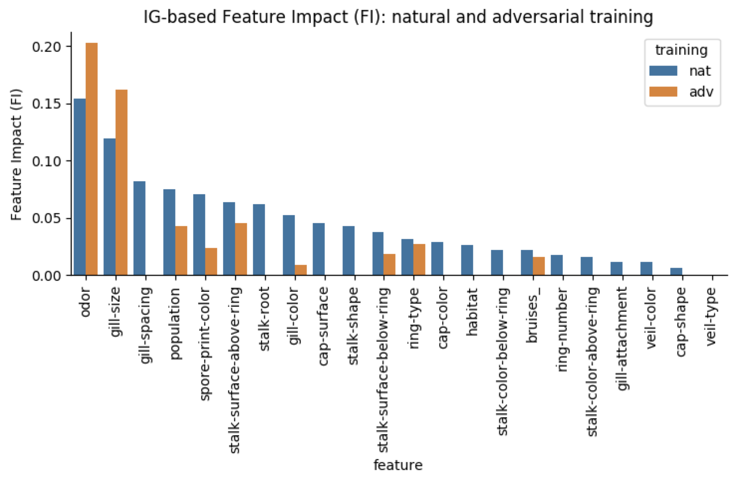
Refer to caption
Figure J.5: Comparison of aggregate Feature Impact (FI) for a naturally-trained model, and an adversarially-trained model with ε=0.1𝜀0.1\varepsilon=0.1, on the mushroom dataset. The features are arranged left to right in decreasing order of the FI value in the naturally-trained model.

J.3 Spambase: Average IG-based Feature Impact

We fix ε=0.1𝜀0.1\varepsilon=0.1 for adversarial training and show in Figure J.6 a bar-plot comparing the average Feature-Impacts (FI), between naturally-trained and adversarially-trained models. Note how the adversarially trained model has significantly fewer features with non-negligible impacts, compared to a naturally trained model.
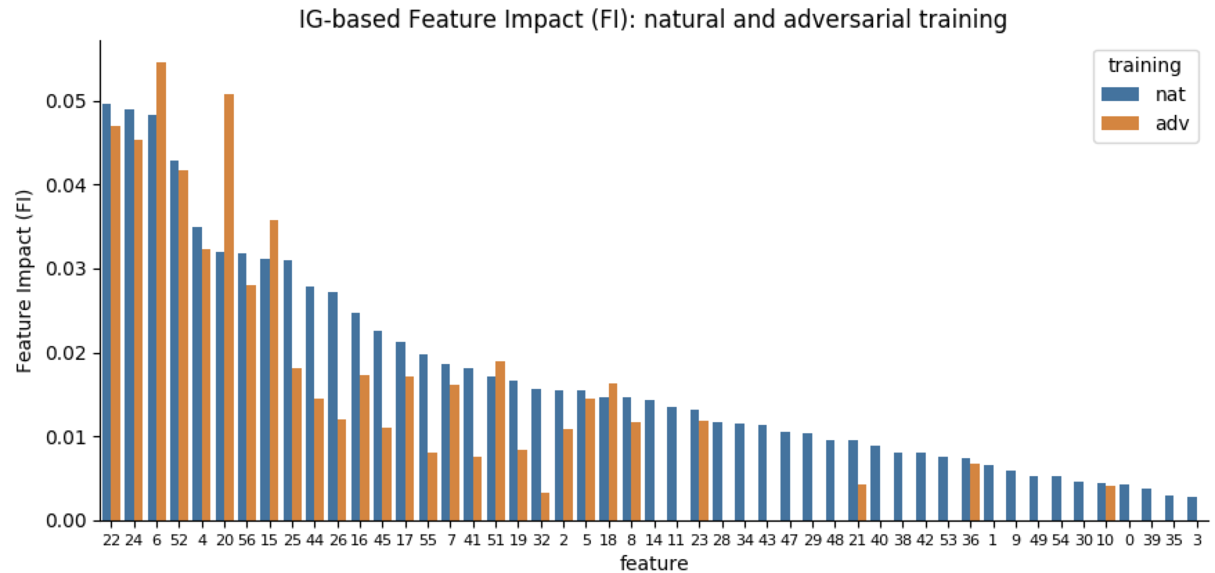
Refer to caption
Figure J.6: Comparison of aggregate Feature Impact (FI) for a naturally-trained model, and an adversarially-trained model with ε=0.1𝜀0.1\varepsilon=0.1, on the spambase dataset. The features are arranged left to right in decreasing order of their FI in the naturally-trained model. To avoid clutter, we show only features that have an FI at least 5% of the highest FI (across both models).

J.4 MNIST, Fashion-MNIST and CIFAR-10: examples

Figs. J.8, J.10 and J.12 below show IG-based saliency maps of images correctly classified by three model types: Naturally trained un-regularized model, naturally trained model with 1subscript1\ell_{1}-regularization, and an (ε)subscript𝜀\ell_{\infty}(\varepsilon)-adversarially trained model. The values of λ𝜆\lambda and ε𝜀\varepsilon are those indicated in Table 1. In each example, all three models predict the correct class with high probability, and we compare the Gini Indices of the IG-vectors (with respect to the predicted probability of the true class). The sparseness of the saliency maps of the adversarially-trained models is visually striking compared to those of the other two models, and this is reflected in the Gini Indices as well. Figs. J.14 and J.16 show analogous results, but using the DeepSHAP (Lundberg & Lee, 2017) attribution method instead of IG. The effect of adversarial training on the sparseness of the saliency maps is even more visually striking when using DeepSHAP, compared to IG (We had difficulty running DeepSHAP on CIFAR-10 data, so we are only able to show results for DeepSHAP on MNIST and Fashion-MNIST).

Natural Training    L1-norm RegularizationAdversarial Training

Refer to caption
Refer to caption
Gini: 0.9271
Refer to caption
Gini: 0.9266
Refer to caption
Gini: 0.9728
(a) For all images, the models give correct prediction – 6.
Refer to caption
Refer to caption
Gini: 0.8112
Refer to caption
Gini: 0.8356
Refer to caption
Gini: 0.9383
(b) For all images, the models give correct prediction – 3.
Refer to caption
Refer to caption
Gini: 0.9315
Refer to caption
Gini: 0.9366
Refer to caption
Gini: 0.9738
(c) For all images, the models give correct prediction – 4.
Refer to caption
Refer to caption
Gini: 0.8843
Refer to caption
Gini: 0.8807
Refer to caption
Gini: 0.9595
(d) For all images, the models give correct prediction – 2.
Figure J.8: Some examples on MNIST. We can see the saliency maps (also called feature importance maps), computed via IG, of adversarially trained model are much sparser compared to other models.

Natural Training    L1-norm RegularizationAdversarial Training

Refer to caption
Refer to caption
Gini: 0.8190
Refer to caption
Gini: 0.8183
Refer to caption
Gini: 0.8532
(a) For all images, the models give correct prediction – Dress.
Refer to caption
Refer to caption
Gini: 0.5777
Refer to caption
Gini: 0.5925
Refer to caption
Gini: 0.7024
(b) For all images, the models give correct prediction – Pullover.
Refer to caption
Refer to caption
Gini: 0.7698
Refer to caption
Gini: 0.7784
Refer to caption
Gini: 0.7981
(c) For all images, the models give correct prediction – Bag.
Refer to caption
Refer to caption
Gini: 0.6840
Refer to caption
Gini: 0.6899
Refer to caption
Gini: 0.7503
(d) For all images, the models give correct prediction – T-shirt.
Figure J.10: Some examples on Fashion-MNIST. We can see the saliency maps (also called feature importance maps), computed via IG, of adversarially trained model are much sparser compared to other models.

Natural Training    L1-norm RegularizationAdversarial Training

Refer to caption
Refer to caption
Gini: 0.6395
Refer to caption
Gini: 0.6556
Refer to caption
Gini: 0.7309
(a) For all images, the models give correct prediction – automobile.
Refer to caption
Refer to caption
Gini: 0.5736
Refer to caption
Gini: 0.6175
Refer to caption
Gini: 0.6914
(b) For all images, the models give correct prediction – airplane.
Refer to caption
Refer to caption
Gini: 0.5505
Refer to caption
Gini: 0.5844
Refer to caption
Gini: 0.6778
(c) For all images, the models give correct prediction – ship.
Refer to caption
Refer to caption
Gini: 0.6150
Refer to caption
Gini: 0.6198
Refer to caption
Gini: 0.7084
(d) For all images, the models give correct prediction – bird.
Figure J.12: Some examples on CIFAR-10. We can see the saliency maps (also called feature importance maps), computed via IG, of adversarially trained model are much sparser compared to other models.

Natural Training    L1-norm RegularizationAdversarial Training

Refer to caption
Refer to caption
Gini: 0.8982
Refer to caption
Gini: 0.9000
Refer to caption
Gini: 0.9528
(a) For all images, the models give correct prediction – 0.
Refer to caption
Refer to caption
Gini: 0.9156
Refer to caption
Gini: 0.9156
Refer to caption
Gini: 0.9685
(b) For all images, the models give correct prediction – 7.
Refer to caption
Refer to caption
Gini: 0.9373
Refer to caption
Gini: 0.9452
Refer to caption
Gini: 0.9773
(c) For all images, the models give correct prediction – 3.
Refer to caption
Refer to caption
Gini: 0.9476
Refer to caption
Gini: 0.9473
Refer to caption
Gini: 0.9825
(d) For all images, the models give correct prediction – 5.
Figure J.14: Some examples on MNIST. We can see the saliency maps (also called feature importance maps), computed via DeepSHAP, of adversarially trained model are much sparser compared to other models.

Natural Training    L1-norm RegularizationAdversarial Training

Refer to caption
Refer to caption
Gini: 0.6749
Refer to caption
Gini: 0.6676
Refer to caption
Gini: 0.7435
(a) For all images, the models give correct prediction – Pullover.
Refer to caption
Refer to caption
Gini: 0.8322
Refer to caption
Gini: 0.8628
Refer to caption
Gini: 0.8953
(b) For all images, the models give correct prediction – Trouser.
Refer to caption
Refer to caption
Gini: 0.8343
Refer to caption
Gini: 0.8374
Refer to caption
Gini: 0.8683
(c) For all images, the models give correct prediction – Bag.
Refer to caption
Refer to caption
Gini: 0.7701
Refer to caption
Gini: 0.7575
Refer to caption
Gini: 0.7920
(d) For all images, the models give correct prediction – Ankle boot.
Figure J.16: Some examples on Fashion-MNIST. We can see the saliency maps (also called feature importance maps), computed via DeepSHAP, of adversarially trained model are much sparser compared to other models.