STARRY: Analytic Occultation Light Curves

Abstract

We derive analytic, closed form, numerically stable solutions for the total flux received from a spherical planet, moon or star during an occultation if the specific intensity map of the body is expressed as a sum of spherical harmonics. Our expressions are valid to arbitrary degree and may be computed recursively for speed. The formalism we develop here applies to the computation of stellar transit light curves, planetary secondary eclipse light curves, and planet-planet/planet-moon occultation light curves, as well as thermal (rotational) phase curves. In this paper we also introduce starry, an open-source package written in C++ and wrapped in Python that computes these light curves. The algorithm in starry is six orders of magnitude faster than direct numerical integration and several orders of magnitude more precise. starry also computes analytic derivatives of the light curves with respect to all input parameters for use in gradient-based optimization and inference, such as Hamiltonian Monte Carlo (HMC), allowing users to quickly and efficiently fit observed light curves to infer properties of a celestial body’s surface map.

1 Introduction

Our understanding of the surface of Earth and the other planets in our solar system starts with the creation of maps. Mapping the colors, compositions, and surface features gives us an understanding of the geological, hydrological, and meteorological processes at play that are the basis of planetary science, including comparative planetology. With the discovery of planets orbiting other stars, cartography becomes a formidable task: these planets are too distant to resolve their surfaces into maps as we do for our own planetary suite. One way to overcome this drawback is to utilize the time-dependence of unresolved, disk-integrated light from planetary bodies: both rotational variability (Russell, 1906; Lacis & Fix, 1972; Cowan & Agol, 2008; Oakley & Cash, 2009) and occultations (Williams et al., 2006; Rauscher et al., 2007) yield the opportunity to constrain the presence of static variations in the surface features of exoplanets.

The first application of time-dependent mapping to exoplanets was carried out in the infrared with the hot Jupiter HD 189733b using both phase variations and secondary eclipses of the exoplanet (Knutson et al., 2007; Majeau et al., 2012; de Wit et al., 2012). These yielded crude constraints on the monopole and dipole components of the thermal emission from the thick, windy atmosphere of this giant planet. Since then, phase curve and/or secondary eclipse measurements have been made for hundreds of other exoplanets (e.g., Shabram et al., 2016; Jansen & Kipping, 2017; Adams & Laughlin, 2018) and have allowed for the measurements of their average albedos and, in some cases, higher order spatial features such as hotspot offsets. Given its unprecedented photometric precision in the thermal infrared, the upcoming James Webb Space Telescope (JWST) is expected to dramatically push the boundaries of what can be inferred from these observations, potentially leading to the construction of de facto surface maps of planets in short orbital periods (Beichman et al., 2014; Schlawin et al., 2018). Future mission concepts such as the Large UV-Optical-InfraRed telescope (LUVOIR) and the Origins Space Telescope (OST) will likewise open doors for the mapping technique, extending it to the study of exoplanets with solid or even liquid surfaces (e.g., Kawahara & Fujii, 2010, 2011; Fujii & Kawahara, 2012; Cowan et al., 2012, 2013; Cowan & Fujii, 2017; Fujii et al., 2017; Luger et al., 2017; Berdyugina & Kuhn, 2017). Future direct imaging telescopes should also enable eclipse mapping from mutual transits of binary planets or planet-moon systems (Cabrera & Schneider, 2007), in analogy with mutual events viewed in the Solar System (Brinkmann, 1973; Vermilion et al., 1974; Herzog & Beebe, 1975; Brinkmann, 1976; Reinsch, 1994; Young et al., 1999, 2001; Livengood et al., 2011).

As we prepare to perform these observations, it is essential that we have robust models of exoplanet light curves so that we may reliably infer the surface maps that generated them. Because the features that we seek will likely be close to the limit of detectability, exoplanet mapping is necessarily a probabilistic problem, requiring a careful statistical approach capable of characterizing the uncertainty on the inferred map. Recently, Farr et al. (2018) introduced exocartographer, a Bayesian model for inferring surface maps and rotation states of exoplanets directly imaged in reflected light. In a similar but complementary vein, Louden & Kreidberg (2018) presented spiderman, a fast code to model phase curves and secondary eclipses of exoplanets, which the authors show is fast enough to be used in Markov Chain Monte Carlo (MCMC) runs for general mapping problems. However, both algorithms, along with all others in the literature to date, rely on numerical integration methods to compute the flux received from the planet during occultation. In addition to the potential loss of precision due to the approximations they employ, numerical algorithms are typically much slower than an analytic approach, should it exist. During the writing of this paper, Haggard & Cowan (2018) derived analytic solutions to the phase curve problem, demonstrating that an exoplanet’s phase curve can be computed exactly in both thermal and reflected light if its map is expressed as a sum of spherical harmonics.

Here we present an algorithm to compute analytic occultation light curves of stars, planets, or moons of arbitrary complexity if the surface map of the occulted body is expressed in the spherical harmonic basis. Our algorithm generalizes the Mandel & Agol (2002), Giménez (2006), and Pál (2012) analytic transit formulae to model eclipses and occultations of bodies with arbitrary, non-radially symmetric surface maps or stars with limb darkening of arbitrary order. For radially symmetric, second-degree maps, our expressions reduce to the Mandel & Agol (2002) quadratic limb darkening transit model; in the limit of zero occultor size or large impact parameter, they reduce to the expressions of Haggard & Cowan (2018) for thermal phase curves.

This paper is organized as follows: in §2 we discuss the real spherical harmonics and introduce our mathematical formalism for dealing with spherical harmonic surface maps. In §3 we discuss how to compute analytic thermal phase curves and occultation light curves for these surface maps. In §4 we introduce our light curve code, starry, and discuss how to use it to compute full light curves for systems of exoplanets and other celestial bodies. We present important caveats in §5 and conclude in §6. Most of the math, including the derivations of the analytic expressions for the light curves, is folded into the Appendix. For convenience, throughout the paper we provide links to Python code (  ) to reproduce all of the figures, as well as links to Jupyter notebooks (  ) containing proofs and derivations of the principal equations. Finally, Table LABEL:tab:symbols at the end lists all the symbols used in the paper, with references to the equations defining them.

2 Surface Maps

In this section we discuss the mathematical framework we use to express, manipulate, and rotate spherical harmonic surface maps. We also introduce two bases, along with corresponding transformations, that will come in handy when computing light curves in §3: the polynomial basis and the Green’s basis. While it is convenient to express a surface map as a set of spherical harmonic coefficients, we will see that it is much easier to integrate the map if we first transform to the appropriate basis.

2.1 Spherical harmonics

The orthonormal real spherical harmonics $Y_{lm}(\uptheta,\upphi)$ of degree $l\geq 0$ and order $m\in[-l,\,l]$ with the Condon-Shortley phase factor (e.g. Varshalovich et al., 1988) are defined in spherical coordinates as

$$Y_{lm}(\uptheta,\upphi)=\begin{cases}\bar{P}_{lm}(\cos\uptheta)\cos(m\upphi)&\qquad m\geq 0\\ \bar{P}_{l|m|}(\cos\uptheta)\sin(|m|\upphi)&\qquad m<0\hskip 0.0pt,\end{cases}$$ (1)

where $\bar{P}_{lm}$ are the normalized associated Legendre functions (Equation A2). On the surface of the unit sphere, we have

$$x =\sin\uptheta\cos\upphi$$

$$y =\sin\uptheta\sin\upphi$$

$$z =\cos\uptheta\hskip 0.0pt,$$ (2)

where $\uptheta$ is the inclination angle and $\upphi$ is the azimuthal angle (ISO convention). The observer is located along the $z$-axis at $z=\infty$ such that the projected disk of the body sits at the origin on the $xy$-plane with $\mathbf{\hat{x}}$ to the right and $\mathbf{\hat{y}}$ up.

Figure 1: The real spherical harmonics up to degree $l=5$ computed from Equation (1). In these plots, the $x$-axis points to the right, the $y$-axis points up, and the $z$-axis points out of the page.     

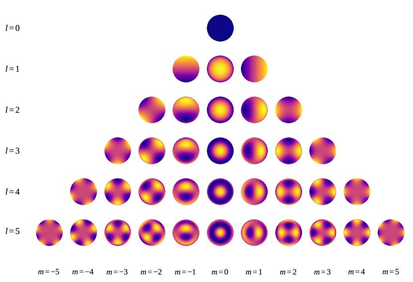
Re-writing Equation (1) in terms of $x$, $y$, and $z$ leads to expressions that are simply polynomials of these variables, a fact we will heavily exploit below when computing their integrals. We derive the polynomial representation of the spherical harmonics in Appendix A. The spherical harmonics up to degree $l=5$ are shown in Figure 1.

2.2 Surface map vectors

Any physical surface map of a celestial body can be expanded in terms of the real spherical harmonics defined in the previous section. For convenience, in this paper we represent a surface map as a vector ${\mathbf{y}}$ of spherical harmonic coefficients such that the specific intensity at the point $(\mbox{$x$},\mbox{$y$})$ may be written

$$I(\mbox{$x$},\mbox{$y$})=\tilde{{\mathbf{y}}}^{\mathsf{T}}(\mbox{$x$},\mbox{$y$})\,{\mathbf{y}}\hskip 0.0pt,$$ (3)

where $\tilde{{\mathbf{y}}}$ is the spherical harmonic basis, arranged in increasing degree and order:

$$\tilde{{\mathbf{y}}}=\begin{pmatrix}Y_{0,0}&Y_{1,-1}&Y_{1,0}&Y_{1,1}&Y_{2,-2}&Y_{2,-1}&Y_{2,0}&Y_{2,1}&Y_{2,2}&\cdot\cdot\cdot\end{pmatrix}^{\mathsf{T}}\hskip 0.0pt,$$ (4)

where $Y_{l,m}=Y_{l,m}(\mbox{$x$},\mbox{$y$})$ are given by Equation (A9). For reference, in this basis the coefficient of the spherical harmonic $Y_{l,m}$ is located at the index

$$n=l^{2}+l+m$$ (5)

of the vector ${\mathbf{y}}$. Conversely, the coefficient at index $n$ of ${\mathbf{y}}$ corresponds to the spherical harmonic of degree and order given by

$$l =\left\lfloor\sqrt{n}\right\rfloor$$

$$m =n-\left\lfloor\sqrt{n}\right\rfloor^{2}-\left\lfloor\sqrt{n}\right\rfloor\hskip 0.0pt,$$ (6)

where $\left\lfloor\scaleto{\cdot}{6pt}\right\rfloor$ is the floor function.

2.3 Change of basis

In order to compute the occultation light curve for a body with a given surface map ${\mathbf{y}}$, it is convenient to first find its polynomial representation ${\mathbf{p}}$, which we express as a vector of coefficients in the polynomial basis $\tilde{{\mathbf{p}}}$:

$$\tilde{p}_{n} =\begin{dcases}\mbox{$x$}^{\frac{\mu}{2}}\mbox{$y$}^{\frac{\nu}{2}}&\qquad\nu\,\mathrm{even}\\ \mbox{$x$}^{\frac{\mu-1}{2}}\mbox{$y$}^{\frac{\nu-1}{2}}\mbox{$z$}&\qquad\nu\,\mathrm{odd}\end{dcases}$$

$$\tilde{{\mathbf{p}}} =\begin{pmatrix}1&\mbox{$x$}&\mbox{$z$}&\mbox{$y$}&\mbox{$x$}^{2}&\mbox{$x$}\mbox{$z$}&\mbox{$x$}\mbox{$y$}&\mbox{$y$}\mbox{$z$}&\mbox{$y$}^{2}&\cdot\cdot\cdot\end{pmatrix}^{\mathsf{T}}\hskip 0.0pt,$$  (7)

where

$$\mu =l-m$$

$$\nu =l+m\hskip 0.0pt$$ (8)

with $l$ and $m$ given by Equation ((LABEL:lm)). To find ${\mathbf{p}}$ given ${\mathbf{y}}$, we introduce the change of basis matrix ${\mathbf{A_{1}}}$, which transforms a vector in the spherical harmonic basis $\tilde{{\mathbf{y}}}$ to the polynomial basis $\tilde{{\mathbf{p}}}$:

$${\mathbf{p}}={\mathbf{A_{1}}}\,{\mathbf{y}}$$ (9)

The columns of ${\mathbf{A_{1}}}$ are simply the polynomial vectors corresponding to each of the spherical harmonics in Equation ((LABEL:by)); see Appendix B for details. As before, the specific intensity at the point $(\mbox{$x$},\mbox{$y$})$ may be computed as

$$I(\mbox{$x$},\mbox{$y$}) =\tilde{{\mathbf{p}}}^{\mathsf{T}}{\mathbf{p}}$$

$$=\tilde{{\mathbf{p}}}^{\mathsf{T}}{\mathbf{A_{1}}}\,{\mathbf{y}}\hskip 0.0pt.$$ (10)

As we will see in the next section, integrating the surface map over the disk of the body is easier if we apply one final transformation to our input vector, rotating it into what we will refer to as the Green’s basis, $\tilde{{\mathbf{g}}}$:

$$\tilde{g}_{n} =\begin{dcases}\frac{\mu+2}{2}\mbox{$x$}^{\frac{\mu}{2}}\mbox{$y$}^{\frac{\nu}{2}}&\qquad\nu\,\mathrm{even}\\[10.00002pt] \mbox{$z$}&\qquad l=1,\,m=0\\[10.00002pt] 3\mbox{$x$}^{l-2}\mbox{$y$}\mbox{$z$}&\qquad\nu\,\mathrm{odd},\,\mu=1,\,l\,\mathrm{even}\\[10.00002pt] \mbox{$z$}\bigg{(}-\mbox{$x$}^{l-3}+\mbox{$x$}^{l-1}+4\mbox{$x$}^{l-3}\mbox{$y$}^{2}\bigg{)}&\qquad\nu\,\mathrm{odd},\,\mu=1,\,l\,\mathrm{odd}\\[10.00002pt] \mbox{$z$}\bigg{(}\frac{\mu-3}{2}\mbox{$x$}^{\frac{\mu-5}{2}}\mbox{$y$}^{\frac{\nu-1}{2}}-\frac{\mu-3}{2}\mbox{$x$}^{\frac{\mu-5}{2}}\mbox{$y$}^{\frac{\nu+3}{2}}-\frac{\mu+3}{2}\mbox{$x$}^{\frac{\mu-1}{2}}\mbox{$y$}^{\frac{\nu-1}{2}}\bigg{)}&\qquad\mathrm{otherwise}\end{dcases}$$

$$\tilde{{\mathbf{g}}} =\begin{pmatrix}1&2\mbox{$x$}&\mbox{$z$}&\mbox{$y$}&3\mbox{$x$}^{2}&-3\mbox{$x$}\mbox{$z$}&2\mbox{$x$}\mbox{$y$}&3\mbox{$y$}\mbox{$z$}&\mbox{$y$}^{2}&\cdot\cdot\cdot\end{pmatrix}^{\mathsf{T}}\hskip 0.0pt,$$  (11)

where the values of $l$, $m$, $\mu$, and $\nu$ are given by Equations (2.2) and (2.3). Given a polynomial vector ${\mathbf{p}}$, the corresponding vector in the Green’s basis, ${\mathbf{g}}$, can be found by performing another change of basis operation:

$${\mathbf{g}}={\mathbf{{\mathbf{A_{2}}}}}\,{\mathbf{p}}$$ (12)

where the columns of the matrix ${\mathbf{A_{2}}}$ are the Green’s vectors corresponding to each of the polynomial terms in Equation ((LABEL:bp)); see Appendix B for details.

Note that we may also transform directly from the spherical harmonic basis to the Green’s basis:

$${\mathbf{g}} ={\mathbf{A_{2}}}\,{\mathbf{A_{1}}}\,{\mathbf{y}}$$

$$={\mathbf{A}}\,{\mathbf{y}}$$ (13)

where

$${\mathbf{A}}\equiv{\mathbf{A_{2}}}\,{\mathbf{A_{1}}}$$ (14)

is the full change of basis matrix. For completeness, we again note that the specific intensity at a point on a map described by the spherical harmonic vector ${\mathbf{y}}$ may be written

$$I(\mbox{$x$},\mbox{$y$}) =\tilde{{\mathbf{g}}}^{\mathsf{T}}(\mbox{$x$},\mbox{$y$}){\mathbf{g}}$$

$$=\tilde{{\mathbf{g}}}^{\mathsf{T}}(\mbox{$x$},\mbox{$y$}){\mathbf{A}}\,{\mathbf{y}}\hskip 0.0pt.$$ (15)

2.4 Rotation of surface maps

Defining a map as a vector of spherical harmonic coefficients makes it straightforward to compute the projection of the map under arbitrary rotations of the body via a rotation matrix ${\mathbf{R}}$:

$${\mathbf{y^{\prime}}}={\mathbf{R}}\,{\mathbf{y}}$$ (16)

where ${\mathbf{y^{\prime}}}$ are the spherical harmonic coefficients of the rotated map. In Appendix C we derive expressions for ${\mathbf{R}}$ in terms of the Euler angles $\alpha$, $\beta$, and $\gamma$, as well as in terms of an angle $\theta$ and an arbitrary axis of rotation ${\mathbf{u}}$. Follow the link next to Figure 1 to view an animation of the spherical harmonics rotating about the $y$-axis, computed from Equation ((LABEL:rotation)).

3 Computing light curves

3.1 Rotational phase curves

Consider a body of unit radius centered at the origin, with an observer located along the $z$-axis at $z=\infty$. The body has a surface map given by the spherical harmonic vector ${\mathbf{y}}$ viewed at an orientation specified by the rotation matrix ${\mathbf{R}}$, such that the specific intensity at a point $(\mbox{$x$},\mbox{$y$})$ on the surface is

$$I(\mbox{$x$},\mbox{$y$}) =\tilde{{\mathbf{y}}}^{\mathsf{T}}(\mbox{$x$},\mbox{$y$}){\mathbf{R}}\,{\mathbf{y}}$$

$$=\tilde{{\mathbf{p}}}^{\mathsf{T}}(\mbox{$x$},\mbox{$y$}){\mathbf{A_{1}}}\,{\mathbf{R}}\,{\mathbf{y}}\hskip 0.0pt$$ (17)

where $\tilde{{\mathbf{p}}}$ is the polynomial basis and ${\mathbf{A_{1}}}$ is the corresponding change-of-basis matrix (§2.3). The total flux radiated in the direction of the observer is obtained by integrating the specific intensity over a region $S$ of the projected disk of the body:

$$F =\oiint I(\mbox{$x$},\mbox{$y$})\,\mathrm{d}S$$

$$=\oiint\tilde{{\mathbf{p}}}^{\mathsf{T}}(\mbox{$x$},\mbox{$y$}){\mathbf{A_{1}}}\,{\mathbf{R}}\,{\mathbf{y}}\,\mathrm{d}S$$

$$={\mathbf{r}}^{\mathsf{T}}{\mathbf{A_{1}}}\,{\mathbf{R}}\,{\mathbf{y}}\hskip 0.0pt,$$ (18)

where ${\mathbf{A_{1}}}$, ${\mathbf{R}}$, and ${\mathbf{y}}$ are constant and ${\mathbf{r}}$ is a column vector whose $n^{\mathrm{th}}$ component is given by

$$r_{n} \equiv\oiint\tilde{p}_{n}(\mbox{$x$},\mbox{$y$})\,\mathrm{d}S\hskip 0.0pt.$$ (19)

When the entire disk of the body is visible (i.e., when no occultation is occurring), this may be written

$$r_{n} =\int_{-1}^{1}\int_{-\sqrt{1-\mbox{$x$}^{2}}}^{\sqrt{1+\mbox{$x$}^{2}}}\tilde{p}_{n}(\mbox{$x$},\mbox{$y$})\,\mathrm{d}\mbox{$y$}\,\mathrm{d}\mbox{$x$}$$

$$=\begin{dcases}\frac{\Gamma\left(\frac{\mu}{4}+\frac{1}{2}\right)\Gamma\left(\frac{\nu}{4}+\frac{1}{2}\right)}{\Gamma\left(\frac{\mu+\nu}{4}+2\right)}&\qquad\frac{\mu}{2}\,\mathrm{even},\,\frac{\nu}{2}\,\mathrm{even}\\[10.00002pt] \frac{\sqrt{\pi}}{2}\frac{\Gamma\left(\frac{\mu}{4}+\frac{1}{4}\right)\Gamma\left(\frac{\nu}{4}+\frac{1}{4}\right)}{\Gamma\left(\frac{\mu+\nu}{4}+2\right)}&\qquad\frac{\mu-1}{2}\,\mathrm{even},\,\frac{\nu-1}{2}\,\mathrm{even}\\[10.00002pt] 0&\qquad\mathrm{otherwise.}\end{dcases}$$  (20)

where $\Gamma(\scaleto{\cdot}{6pt})$ is the gamma function. Equation ((LABEL:phaseint)) may be used to analytically compute the rotational (thermal) phase curve of a body with an arbitrary surface map. Since ${\mathbf{r}}$ and ${\mathbf{A_{1}}}$ are independent of the map coefficients or its orientation, these may be pre-computed for computational efficiency.

We note, finally, that a form of this solution was very recently found by Haggard & Cowan (2018); a special case of their equations for phase curves in reflected light yields analytic expressions for thermal phase curves of spherical harmonics.

3.2 Occultation light curves

As we showed earlier, the specific intensity at a point $(\mbox{$x$},\mbox{$y$})$ on the surface of a body described by the map ${\mathbf{y}}$ and the rotation matrix $\vec{R}$ may also be written as

$$I(\mbox{$x$},\mbox{$y$}) =\tilde{{\mathbf{y}}}^{\mathsf{T}}(\mbox{$x$},\mbox{$y$}){\mathbf{R}}\,{\mathbf{y}}$$

$$=\tilde{{\mathbf{g}}}^{\mathsf{T}}(\mbox{$x$},\mbox{$y$}){\mathbf{A}}\,{\mathbf{R}}\,{\mathbf{y}}\hskip 0.0pt,$$ (21)

where $\tilde{{\mathbf{g}}}$ is the Green’s basis and ${\mathbf{A}}$ is the full change of basis matrix (§2.3). As before, the total flux radiated in the direction of the observer is obtained by integrating the specific intensity over a region $S$ of the projected disk of the body:

$$F =\oiint I(\mbox{$x$},\mbox{$y$})\,\mathrm{d}S$$

$$=\oiint\tilde{{\mathbf{g}}}^{\mathsf{T}}(\mbox{$x$},\mbox{$y$})\,\mathrm{d}S\,{\mathbf{A}}\,{\mathbf{R}}\,{\mathbf{y}}\hskip 0.0pt.$$ (22)

This time, suppose the body is occulted by another body of radius $r$ centered at the point $(x_{o},y_{o})$, so that the surface $S$ over which the integral is taken is a function of $r$, $x_{o}$, and $y_{o}$. In general, the integral in Equation ((LABEL:occint)) is difficult (and often impossible) to compute directly. One way to simplify the problem is to first perform a rotation through an angle

$$\omega=\frac{\pi}{2}-\mathrm{arctan2}(y_{o},x_{o})$$ (23)

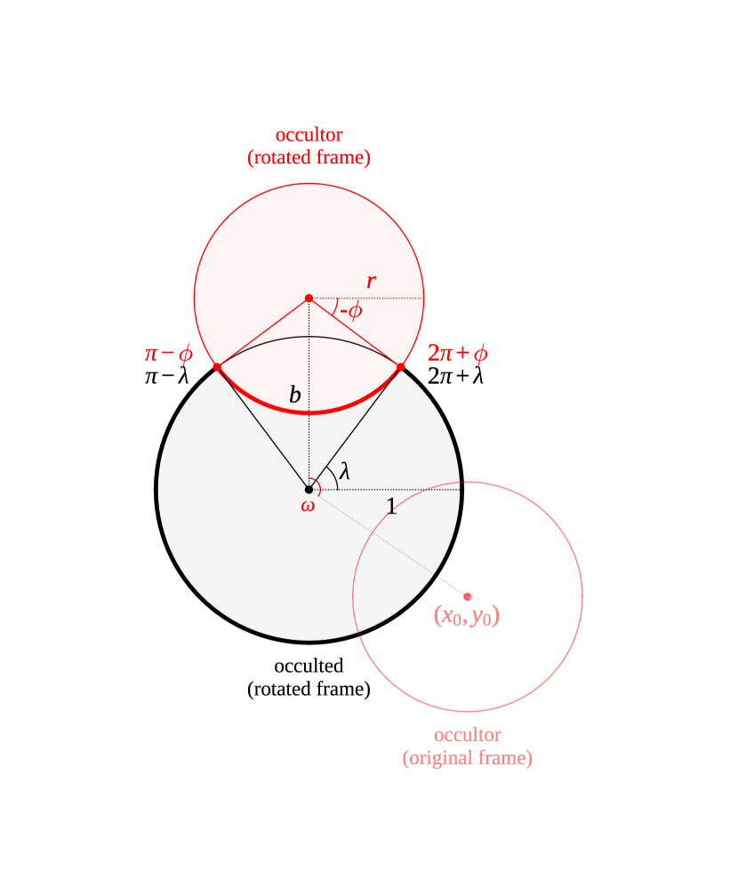
about the $z$-axis (${\mathbf{u}}=\left[0,0,1\right]$) so that the occultor lies along the $+y$-axis, with its center located a distance $b=\sqrt{x_{o}^{2}+y_{o}^{2}}$ from the origin (see Figure 2). In this rotated frame, the limits of integration (the two points of intersection between the occultor and the occulted body, should they exist) are symmetric about the $y$-axis. If we define $\phi\in[-\nicefrac{{\pi}}{{2}},\,\nicefrac{{\pi}}{{2}}]$ as the angular position of the right hand side intersection point relative to the occultor center, measured counter-clockwise from the $+x$ direction, the arc of the occultor that overlaps the occulted body extends from $\pi-\phi$ to $2\pi+\phi$ (see the Figure). Similarly, defining $\lambda\in[-\nicefrac{{\pi}}{{2}},\,\nicefrac{{\pi}}{{2}}]$ as the angular position of the same point relative to the origin, the arc of the portion of the occulted body that is visible during the occultation extends from $\pi-\lambda$ to $2\pi+\lambda$ (see the Figure). For future reference, it can be shown that

$$\phi =\begin{dcases}\arcsin\left({\frac{1-r^{2}-b^{2}}{2br}}\right)&\qquad|1-r|<b<1+r\\ \frac{\pi}{2}&\qquad b\leq 1-r\end{dcases}$$  (24)

and

$$\lambda =\begin{dcases}\arcsin\left(\frac{1-r^{2}+b^{2}}{2b}\right)&\qquad|1-r|<b<1+r\\ \frac{\pi}{2}&\qquad b\leq 1-r\hskip 0.0pt.\end{dcases}$$  (25)

The case $b\leq 1-r$ corresponds to an occultation during which the occultor is fully within the planet disk, so no points of intersection exist. In this case, we define $\phi$ such that the arc from $\pi-\phi$ to $2\pi+\phi$ spans the entire circumference of the occultor, and $\lambda$ such that the arc from $\pi-\lambda$ to $2\pi+\lambda$ spans the entire circumference of the occulted body. Note that if $b\geq 1+r$, no occultation occurs and the flux may be computed as in §3.1, while if $b\leq r-1$, the entire disk of the body is occulted and the total flux is zero.

The second trick we employ to solve Equation ((LABEL:sn)) is to use Green’s theorem to express the surface integral of $\tilde{{\mathbf{g}}}_{n}$ as the line integral of a vector function ${\mathbf{G}}_{n}$ along the boundary of the same surface (Pál, 2012). Defining the “solution” column vector

$${\mathbf{s}}^{\mathsf{T}} \equiv\oiint\tilde{{\mathbf{g}}}^{\mathsf{T}}(\mbox{$x$},\mbox{$y$})\,\mathrm{d}S\hskip 0.0pt,$$ (26)

we may write its $n^{\mathrm{th}}$ component as

$$s_{n} =\oiint\tilde{g}_{n}(\mbox{$x$},\mbox{$y$})\,\mathrm{d}S=\oint{\mathbf{G}}_{n}(\mbox{$x$},\mbox{$y$})\cdot\mathrm{d}{\mathbf{r}}\hskip 0.0pt,$$ (27)

where ${\mathbf{G}}_{n}(\mbox{$x$},\mbox{$y$})={G_{n}}_{x}(\mbox{$x$},\mbox{$y$})\,\mathbf{\hat{x}}+{G_{n}}_{y}(\mbox{$x$},\mbox{$y$})\,\mathbf{\hat{y}}$ is chosen such that

$${\mathbf{D}}\wedge{\mathbf{G}}_{n}=\tilde{g}_{n}(\mbox{$x$},\mbox{$y$})\hskip 0.0pt.$$ (28)

The operation ${\mathbf{D}}\wedge{\mathbf{G}}_{n}$ denotes the exterior derivative of ${\mathbf{G}}_{n}$. In two-dimensional Cartesian coordinates, it is given by

$${\mathbf{D}}\wedge{\mathbf{G}}_{n} \equiv\frac{\mathrm{d}{G_{n}}_{y}}{\mathrm{d}\mbox{$x$}}-\frac{\mathrm{d}{G_{n}}_{x}}{\mathrm{d}\mbox{$y$}}\hskip 0.0pt.$$ (29)

Thus, in order to compute $s_{n}$ in Equation ((LABEL:greens)), we must (1) apply a rotation to our map ${\mathbf{y}}$ to align the occultor with the $+y$-axis; (2) find a vector function ${\mathbf{G}}_{n}$ whose exterior derivative is the $n^{\mathrm{th}}$ component of the vector basis $\tilde{{\mathbf{g}}}$ (Equation 11); and (3) integrate it along the boundary of the visible portion of the occulted body’s surface. In general, for an occultation involving two bodies, this boundary consists of two arcs: a segment of the circle bounding the occultor (thick red curve in Figure 2), and a segment of the circle bounding the occulted body (thick black curve in Figure 2). If we happen to know ${\mathbf{G}}_{n}$, the integral in Equation ((LABEL:greens)) is just

$$s_{n} =\mathcal{Q}({\mathbf{G}}_{n})-\mathcal{P}({\mathbf{G}}_{n})\hskip 0.0pt,$$ (30)

where, as in Pál (2012), we define the primitive integrals

$$\mathcal{P}({\mathbf{G}}_{n}) =\int\displaylimits_{\pi-\phi}^{2\pi+\phi}\big{[}{G_{n}}_{y}(rc_{\varphi},b+rs_{\varphi})c_{\varphi}-{G_{n}}_{x}(rc_{\varphi},b+rs_{\varphi})s_{\varphi}\big{]}r\mathrm{d}\varphi$$ (31)

and

$$\mathcal{Q}({\mathbf{G}}_{n}) =\int\displaylimits_{\pi-\lambda}^{2\pi+\lambda}\big{[}{G_{n}}_{y}(c_{\varphi},s_{\varphi})c_{\varphi}-{G_{n}}_{x}(c_{\varphi},s_{\varphi})s_{\varphi}\big{]}\mathrm{d}\varphi\hskip 0.0pt,$$ (32)

where we defined $c_{\varphi}\equiv\cos\varphi$ and $s_{\varphi}\equiv\sin\varphi$ and we used the fact that along the arc of a circle,

$$\mathrm{d}{\mathbf{r}} =-rs_{\varphi}\,\mathrm{d}\varphi\,\mathbf{\hat{x}}+rc_{\varphi}\,\mathrm{d}\varphi\,\mathbf{\hat{y}}\hskip 0.0pt.$$ (33)

In Equations (31) and (32), $\mathcal{P}({\mathbf{G}}_{n})$ is the line integral along the arc of the occultor of radius $r$, and $\mathcal{Q}({\mathbf{G}}_{n})$ is the line integral along the arc of the occulted body of radius one.

Figure 2: Geometry of the occultation problem. The occulted body is centered at the origin and has unit radius, while the occultor is centered at $(x_{o},y_{o})$ and has radius $r$. The observer is located at $z=\infty$. We first rotate the two bodies about the origin through an angle $\omega=\nicefrac{{\pi}}{{2}}-\mathrm{arctan2}(y_{o},x_{o})$ so the problem is symmetric about the $y$-axis. In this frame, the occultor is located at $(0,b)$, where $b=\sqrt{x_{o}^{2}+y_{o}^{2}}$ is the impact parameter. The arc of the occultor that overlaps the occulted body (thick red curve) now extends from $\pi-\phi$ to $2\pi+\phi$, measured from the center of the occultor. The arc of the occulted body that is visible during the occultation (thick black curve) extends from $\pi-\lambda$ to $2\pi+\lambda$, measured from the origin. These are the curves along which the primitive integrals (Equations 31 and 32) are evaluated. The angles $\phi$ and $\lambda$ are given by Equations (24) and (25) and extend from $-\nicefrac{{\pi}}{{2}}$ to $\nicefrac{{\pi}}{{2}}$. When the occultor is completely within the disk of the occulted body, we define $\phi=\lambda=\nicefrac{{\pi}}{{2}}$.   

As cumbersome as the Green’s basis (Equation 11) may appear, the reason we introduced it is that its anti-exterior derivatives are conveniently simple. It can be easily shown that one possible solution to Equation ((LABEL:DGg)) is

$${\mathbf{G}}_{n}(\mbox{$x$},\mbox{$y$}) =\begin{dcases}\mbox{$x$}^{\frac{\mu+2}{2}}\mbox{$y$}^{\frac{\nu}{2}}\,\mathbf{\hat{y}}&\qquad\nu\,\mathrm{even}\\[10.00002pt] \frac{1-z^{3}}{3(1-z^{2})}(-\mbox{$y$}\,\mathbf{\hat{x}}+\mbox{$x$}\,\mathbf{\hat{y}})&\qquad l=1,\,m=0\\[10.00002pt] \mbox{$x$}^{l-2}\mbox{$z$}^{3}\,\mathbf{\hat{x}}&\qquad\nu\,\mathrm{odd},\,\mu=1,\,l\,\mathrm{even}\\[10.00002pt] \mbox{$x$}^{l-3}\mbox{$y$}\mbox{$z$}^{3}\,\mathbf{\hat{x}}&\qquad\nu\,\mathrm{odd},\,\mu=1,\,l\,\mathrm{odd}\\[10.00002pt] \mbox{$x$}^{\frac{\mu-3}{2}}\mbox{$y$}^{\frac{\nu-1}{2}}\mbox{$z$}^{3}\,\mathbf{\hat{y}}&\qquad\mathrm{otherwise,}\end{dcases}$$  (34)

where $l$ and $m$ are given by Equation ((LABEL:lm)) and $\mu$ and $\nu$ are given by Equation ((LABEL:munu)). Solving the occultation problem is therefore a matter of evaluating the primitive integrals of ${\mathbf{G}}_{n}$ (Equations 31 and 32). The solutions are in general tedious, but they are all analytic, involving sines, cosines, and complete elliptic integrals. In Appendix D we derive recurrence relations to quickly compute these. We note, in particular, that the solutions all involve complete elliptic integrals of the same argument, so that the elliptic integrals need only be evaluated once for a map of arbitrary degree, greatly improving the evaluation speed and the scalability of the problem to high order. In practice we find that the stability in evaluation of these expressions is improved by using a rapidly converging series expansion for occultors of large and small radius.

3.3 Summary

Here we briefly summarize how to analytically compute the flux during an occultation of a body whose specific intensity profile is described by a sum of spherical harmonics. The first step is to compute the change-of-basis matrix ${\mathbf{A}}$ (§2.3) to convert our vector of spherical harmonic coefficients to a vector of polynomial coefficients in the Green’s basis (Equation 11). Since ${\mathbf{A}}$ is constant, this matrix may be pre-computed for speed.

Then, given a body of unit radius with a surface map described by the vector of spherical harmonic coefficients $\mathbf{y}$ (Equation 4), occulted by another body of radius $r$ centered at the point $(x_{o},y_{o})$, and viewed by an observer located at $z=\infty$, we must:

1. Compute the rotation matrix ${\mathbf{R}}$ to rotate the map to the correct viewing orientation, which may be specified by the Euler angles $\alpha$, $\beta$, and $\gamma$ (Appendix C.1) or by an axis ${\mathbf{u}}$ and an angle $\theta$ (Appendix C.2).

2. Compute the rotation matrix ${\mathbf{R^{\prime}}}$ to rotate the map by an angle $\omega$ about the $+z$-axis (Equation 23) so the center of the occultor is a distance $b=\sqrt{x_{o}^{2}+y_{o}^{2}}$ along the $+y$-axis from the center of the occulted body.

3. Compute the solution vector ${\mathbf{s}}$ (Equation 30), with $\mathcal{P}({\mathbf{G}}_{n})$ and $\mathcal{Q}({\mathbf{G}}_{n})$ given by the equations in Appendix D.2. Note that $s_{2}$ is special and must be computed separately (Equation D1).

Given these quantities, the total flux $f$ during an occultation is then just

$$\boxed{f={\mathbf{s}}^{\boldsymbol{\mathsf{T}}}{\mathbf{A}}\,{\mathbf{R^{\prime}}}\,{\mathbf{R}}\,{\mathbf{y}}}\hskip 0.0pt.$$ (35)

4 The STARRY code package

The starry code package provides code to analytically compute light curves for celestial bodies using the formalism developed in this paper. starry is coded entirely in C++ for speed and wrapped in Python using pybind11 (Jakob et al., 2017) for quick and easy light curve calculations. The code may be installed three different ways: using conda (recommended),

⬇

1conda install -c conda-forge starry

via pip,

⬇

1pip install starry

or from source by cloning the GitHub repository,

⬇

1git clone https://github.com/rodluger/starry.git

2cd starry

3python setup.py develop

There are two primary ways of interfacing with starry: via the surface map class Map and via the celestial body system class kepler.System. The former gives users the most flexibility to create and manipulate surface maps and compute their fluxes for a variety of applications, while the latter provides an easy way to generate light curves for simple Keplerian systems. Let us discuss the map class first.

Figure 3: Rotation of the map given by Equation (36) about $\mathbf{\hat{y}}$.   

4.1 Creating a map

To begin using starry, execute the following in a Python environment:

⬇

1from starry import Map

A starry Map is a vector of spherical harmonic coefficients, indexed by increasing degree and order, as in Equation ((LABEL:by)). As an example, we can create a map of spherical harmonics up to degree $l_{\mathrm{max}}=5$ by typing

⬇

3map = Map(lmax=5)

By default, the first coefficient ($y_{0}$, the coefficient multiplying the $Y_{0,0}$ harmonic) is set to unity and all other coefficients are set to zero. Importantly, maps in starry are normalized such that the average disk-integrated intensity is equal to the coefficient of the $Y_{0,0}$ harmonic. By default, the average amount of flux visible from an unocculted map is therefore unity.

Say our surface map is given by the function

$$I(\mbox{$x$},\mbox{$y$}) =Y_{0,0}-2Y_{5,-3}(\mbox{$x$},\mbox{$y$})+2Y_{5,0}(\mbox{$x$},\mbox{$y$})+Y_{5,4}(\mbox{$x$},\mbox{$y$})\hskip 0.0pt.$$ (36)

To create this map, we set the corresponding coefficients by direct assignment to the (l, m) indices of the Map instance:

⬇

1map[5, -3] = -2

2map[5, 0] = 2

3map[5, 4] = 1

Users can also directly access the spherical harmonic vector ${\mathbf{y}}$, polynomial vector ${\mathbf{p}}$, and Green’s polynomial vector ${\mathbf{g}}$ via the read-only attributes Map.y, Map.p, and Map.g, respectively. Once a map is instantiated, users may quickly visualize it by calling

⬇

3map.show()

or

⬇

3map.animate()

where the editable attribute Map.axis defines the axis of rotation for the animation. Rotation of this map about $\mathbf{\hat{y}}$ yields the sequence shown in Figure 3.

Alternatively, users may provide a two-dimensional numpy array of intensities on a latitude-longitude grid or the path to an image file of the surface map on a latitude-longitude grid:

⬇

3map.load_image(array)

or

⬇

3map.load_image("/path/to/image.jpg")

In both cases, starry uses the map2alm() function of the healpy package to find the expansion of the map in terms of spherical harmonics. Keep in mind that if the image contains very dark pixels (with RGB values close to zero), its spherical harmonic expansion may lead to regions with negative specific intensity, which is of course unphysical.

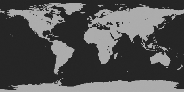
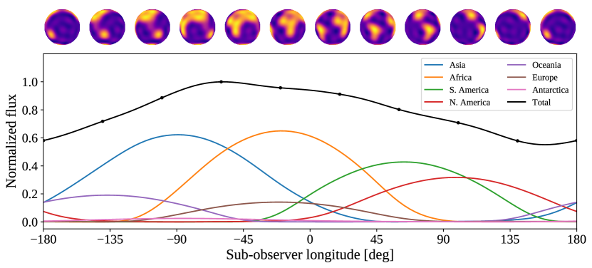
In Figure 4 we show a simplified two-color map of the cloudless Earth and its corresponding starry instance for $l_{\mathrm{max}}=10$, rotated successively about $\mathbf{\hat{y}}$.

Figure 4: A simplified two-color map of the cloudless Earth (top) and the corresponding tenth-degree spherical harmonic expansion, rotated about $\mathbf{\hat{y}}$ (bottom).   

4.2 Computing rotational phase curves

Figure 5: Top: Phase curves for the first several spherical harmonics with order $m\geq 0$ rotated about the $x$-axis (blue) and about the $y$-axis (orange). Odd harmonics with $l>1$ and harmonics with $m<0$ are in the phase curve null space (Cowan et al., 2013). Bottom: Occultation light curves for the same set of harmonics. An occultor of radius $r=0.3$ transits the body along the $+\mbox{$x$}$ direction at $y_{o}=0.25$ (blue) and $y_{o}=0.75$ (orange).     

Once a map is instantiated, it is easy to compute its rotational phase curve, F:

⬇

3F = map.flux(theta=theta)

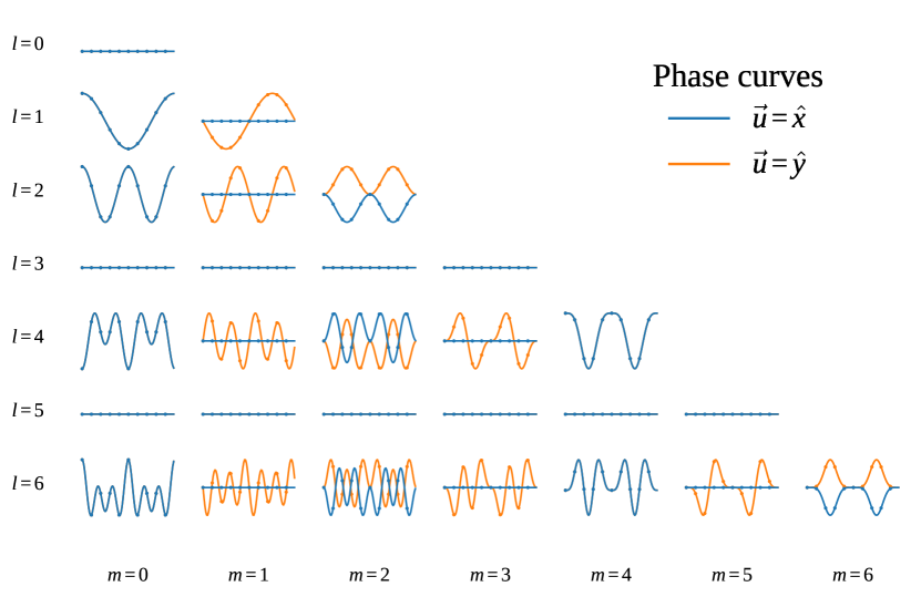
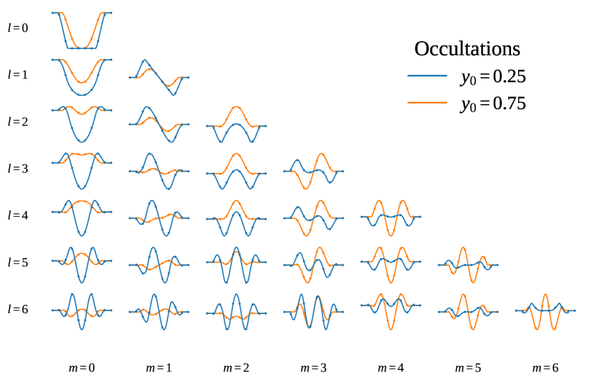
where theta is an array of angles (in degrees) for which to compute the flux. Note that rotations performed by Map.flux() are not cumulative; instead, all angles should be specified relative to the original, unrotated map frame. As before, the axis of rotation can be set via the Map.axis attribute. In the top panel of Figure 5 we plot rotational phase curves for all spherical harmonics up to $l_{\mathrm{max}}=6$ for rotation about $\mathbf{\hat{x}}$ (blue curves) and $\mathbf{\hat{y}}$ (orange curves). The small dots correspond to phase curves computed by numerical evaluation of the flux on an adaptive radial mesh (see §4.7). As discussed by Cowan et al. (2013), harmonics with odd $l>1$ and those with $m<0$ (not plotted) are in the null space and therefore do not exhibit rotational phase variations when rotated about $\mathbf{\hat{x}}$ or $\mathbf{\hat{y}}$.

As a second example, we can compute the rotational phase curve of the simplified Earth model (Figure 4) for rotation about $\mathbf{\hat{y}}$ (its actual spin axis) by executing

⬇

3theta = np.linspace(0, 360, 100)

4F = map.flux(theta=theta)

The variable F is an array of flux values computed from Equation ((LABEL:phaseint)); we plot this in Figure 6, alongside the rotational phase curves due to each of the seven individual continents. For more complex phase curves, such as those of planets on inclined orbits, see §4.5.

Figure 6: Phase curve for the Earth rotating about its axis, computed from the $l_{\mathrm{max}}=10$ expansion from Figure 4. The full rotational phase curve is shown in black, and the flux due to each of the seven continents is shown as the colored curves (see legend). The black dots correspond to the numerical solution (see §4.7).   

4.3 Computing occultation light curves

Occultation light curves are similarly easy to compute:

⬇

3F = map.flux(theta=theta, xo=xo, yo=yo, ro=ro)

where theta is the same as above, and xo, yo, and ro are the occultor parameters ($x$ position, $y$ position, and radius, all in units of the occulted body’s radius), which may be either scalars or arrays.

In the bottom panel of Figure 5 we plot occultation light curves for the spherical harmonics with $m\geq 0$ up to $l_{\mathrm{max}}=6$. The occultor has radius $r=0.3$ and moves at a constant speed along the $x$ direction at $y_{o}=0.25$ (blue curves) and $y_{o}=0.75$ (orange curves). The light curve of any body undergoing such an occultation can be expressed as a weighted sum of these light curves. Note that because the value of individual spherical harmonics can be negative, an increase in the flux is visible at certain points during the occultation; however, this would of course not occur for any physical map constructed from a linear combination of the spherical harmonics. Note also that unlike in the case of rotational phase curves, there is no null space for occultations, as all spherical harmonics (including those with $m<0$, which are not shown) produce a flux signal during occultation. As before, the numerical solutions are shown as the small dots.

Figure 7: Occultation light curve for the Moon transiting the rotating Earth, computed from the $l_{\mathrm{max}}=10$ expansion from Figure 4. The two largest dips are due to the occultations of South America (left) and Africa (right). Once again, the black dots correspond to the numerical solution (see §4.7). For reference, the light grey dots correspond to the rotational light curve in the absence of the occultor.   

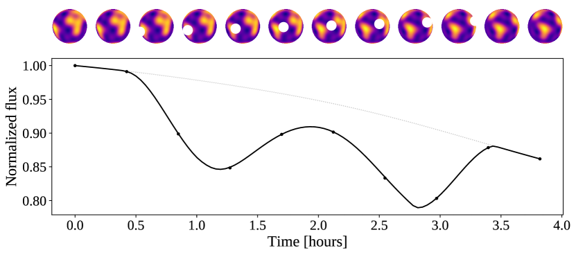
To further illustrate the code, we return to our spherical harmonic expansion of the Earth. Figure 7 shows an occultation light curve computed for a hypothetical transit of the Earth by the Moon. The occultation lasts about four hours, during which time the sub-observer point rotates from Africa to South America, causing a steady flux decrease as the Pacific Ocean rotates into view. The occultation is double-dipped: one dip due to the occultation of South America, and one dip due to the occultation of Africa.

4.4 Computing light curves of limb-darkened bodies

The formalism developed in this paper can easily be extended to the case of occultations of limb-darkened maps (such as transits of planets across stars) by noting that any radially symmetric specific intensity profile can be expressed as a sum over the $m=0$ spherical harmonics (see Figure 1). In particular, Agol & Luger (2018) show how a limb darkening profile that is an order $l$ polynomial function of the radial coordinate, $\upmu=\mbox{$z$}=\sqrt{1-\mbox{$x$}^{2}-\mbox{$y$}^{2}}$, can be exactly expressed in terms of the $m=0$ spherical harmonics up to order $l$.

All Map instances in starry have an additional read-only attribute, Map.u, which stores the limb darkening coefficients $\{u_{1},u_{2},u_{3},...\}$ of the map. These are all zero by default, and can be changed by direct assignment to index l of the map instance:

⬇

4map[1] = u1

5map[2] = u2

6...

7map[lmax] = ulmax

In the case of quadratic limb darkening ($l_{\mathrm{max}}=2$), this sets the map’s limb darkening profile to

$$\frac{I(\upmu)}{I(1)} =1-u_{1}(1-\upmu)-u_{2}(1-\upmu)^{2}\hskip 0.0pt,$$ (37)

with $\upmu$ given above. It is straightforward to show that this corresponds to the spherical harmonic sum

$$\frac{I(\mbox{$x$},\mbox{$y$})}{I(1)}=\frac{2\sqrt{\pi}}{3}(3-3u_{1}-4u_{2})\,Y_{0,0}+\frac{2\sqrt{\pi}}{\sqrt{3}}(u_{1}+2u_{2})\,Y_{1,0}-\frac{4\sqrt{\pi}}{3\sqrt{5}}u_{2}\,Y_{2,0}\hskip 0.0pt,$$  (38)

where we set

$$I(1)=\frac{1}{\pi(1-\frac{1}{3}u_{1}-\frac{1}{6}u_{2})}$$ (39)

to enforce the integral of the specific intensity over the visible disk is unity. Limb darkening profiles of arbitrary degree are supported in starry, and in all cases the corresponding light curve is computed analytically.

Note, importantly, that the limb darkening coefficients are treated separately from the spherical harmonic coefficients in starry. In particular, the limb darkening profile does not rotate along with the rest of the map when a rotation is applied. Moreover, while most users will find it sufficient to specify either the spherical harmonic coefficients or the limb darkening coefficients of a surface map, it is also possible to specify both. This may be convenient in the case of a limb-darkened star with rotating starspots or other surface inhomogeneities. In this case, the limb darkening coefficients are applied to the map as a multiplicative filter following any requested rotation operations. Since products of spherical harmonics are spherical harmonics, applying limb darkening to a spherical harmonic map simply raises its degree by an amount equal to the degree of the limb darkening profile. Hence users must be careful not to exceed the maximum degree of the map when setting limb darkening coefficients. For instance, a map instantiated with lmax=10 having nonzero spherical harmonic coefficients up to degree $l=5$ can have at most fifth order ($l=5$) limb darkening.

In principle, one could also model limb-darkened planetary atmospheres in this fashion, but we do not in general recommend this. Inhomogeneities in the planetary atmosphere could lead to asymmetries in the limb darkening, which should probably be treated using a radiative transfer model.

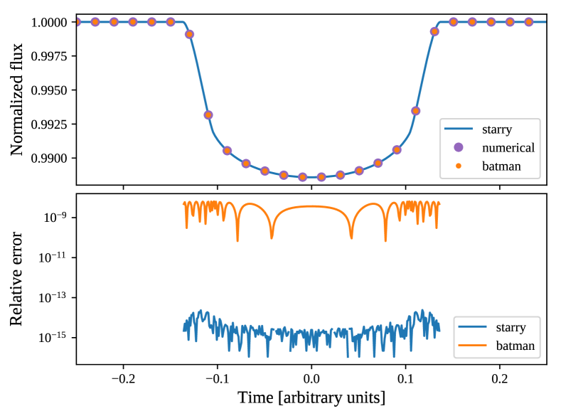
Figure 8 shows the light curve of a planet transit across a quadratically limb-darkened star with $u_{1}=0.4,u_{2}=0.26$ computed using starry. The planet/star radius ratio is $r=0.1$ and the planet transits at impact parameter $b=0.5$. For comparison, we also compute the flux with batman (Kreidberg, 2015) and with a high precision numerical integration of the surface integral of Equation ((LABEL:quadraticld)) using the scipy.integrate.dblquad (Jones et al., 2001) routine with a tolerance of $10^{-14}$. The relative error on the flux for starry flux is less than $10^{-7}$ parts per million everywhere in the light curve.

Figure 8: Sample transit light curve for a planet ($r=0.1$) transiting a quadratically limb-darkened star ($u_{1}=0.4,u_{2}=0.26$). The top panel shows the starry (blue curve) and batman (orange dots) light curves, as well as a light curve generated by a high precision direct numerical integration of the surface integral (purple dots). The bottom panel shows the relative error on the flux compared to the high precision numerical solution for starry (blue) and batman (orange).   

4.5 Photodynamics

The Map class discussed above is convenient when the rotational state of the body in question and/or the position of the occultor is known, or when these can easily be computed by some other means. For convenience, starry implements a Keplerian solver to compute light curves of simple star-planet, star-star, or planet-moon systems given the orbital parameters as input. Users can access this functionality by instantiating a kepler.Primary and any number of kepler.Secondary objects, then passing them to a kepler.System instance. As an example, let us create a central star:

⬇

3from starry.kepler import Primary

4star = Primary(lmax=2)

A kepler.Primary instance has unit radius and unit luminosity; the secondary bodies’ radii, semi-major axes, and luminosities are all defined relative to these values. All kepler.Primary and kepler.Secondary instances derive from the Map class, so we can limb-darken the star in the same way as before:

⬇

7star[1] = 0.40

8star[2] = 0.26

where we arbitrarily set $u_{1}=0.40$ and $u_{2}=0.26$. Next, we will instantiate a planet by typing

⬇

4from starry.kepler import Secondary

5planet = Secondary(lmax=1)

Let us set its orbital parameters as follows:

⬇

8planet.r = 0.1 # Radius in units of primary radius

9planet.L = 5.e-3 # Luminosity in units of primary

10planet.a = 50 # Semi-major axis in units of primary

11planet.inc = 90 # Inclination in degrees

12planet.ecc = 0 # Eccentricity

13planet.w = 90 # Longitude of pericenter in degrees

14planet.Omega = 0 # Longitude of ascending node in degrees

15planet.lambda0 = 90 # Mean longitude in deg. at the ref. time

16planet.tref = 0 # Reference time in days

17planet.porb = 4.3 # Orbital period in days

18planet.prot = 4.3 # Rotational period in days

These properties, along with their default values, are detailed in full in the documentation.

Suppose we wish to give the planet a simple dipole map ($Y_{1,0}$) with peak brightness at the sub-stellar point. starry expects the planet map to be instantiated at an eclipsing configuration (full phase), so we want to set the coefficient for the $Y_{1,0}$ harmonic (see Figure 1):

⬇

5planet[1, 0] = 0.5

Finally, care should be taken to ensure the map is positive everywhere. By default, the coefficient of the $Y_{0,0}$ term of a map is fixed at unity, since changing this term would change the total luminosity (this should instead be modified via the kepler.Secondary.L property). In the case of a simple dipole map of the form $Y_{0,0}\,+\,y_{1}Y_{1,-1}\,+\,y_{2}Y_{1,0}\,+\,y_{3}Y_{1,1}$, it can be shown that as long as we enforce

$$y_{1}^{2}+y_{2}^{2}+y_{3}^{2}\leq\frac{1}{3}$$  (40)

the map will be non-negative everywhere along the unit sphere. Since $0.5^{2}<\nicefrac{{1}}{{3}}$, our map is in fact positive semi-definite. For more details on ensuring surface maps are positive everywhere, see §5.4.

We are now ready to instantiate the planetary system:

⬇

18from starry.kepler import System

19system = System(star, planet)

(note that the primary body must always be listed first). We can now compute the full light curve:

⬇

5system.compute(time)

where time is the array of times (in days) at which to compute the light curve. This command internally calls the Map.flux() method of each of the surface maps, populating the flux attribute of each body with its respective light curve. The total light curve (the sum of the light curves of each of the bodies in the system, including the star) is stored in kepler.System.lightcurve. The top panel of Figure 9 shows the light curve for the system we instantiated above: both the transits and secondary eclipses of the planet are clearly visible. For flair, we added a hotspot offset of $15^{\circ}$ to simulate advection of heat by an eastward wind, causing the peak of the planet’s phase curve to occur slightly before secondary eclipse (refer to the Python script for details).

Figure 9: Sample analytic exoplanet system light curves computed with starry. Top: a hot Jupiter transiting a Sun-like star. The planet’s map is a simple dipole, with the hotspot offset 15^∘ from stellar noon; the offset in the secondary eclipse from the peak of the phase curve is apparent. Bottom: a two-planet system with more complex surface maps. In addition to transits and secondary eclipses, a few planet-planet occultations are visible (e.g., the very short events at $t=0.1$ and $t=3.4$ days).   

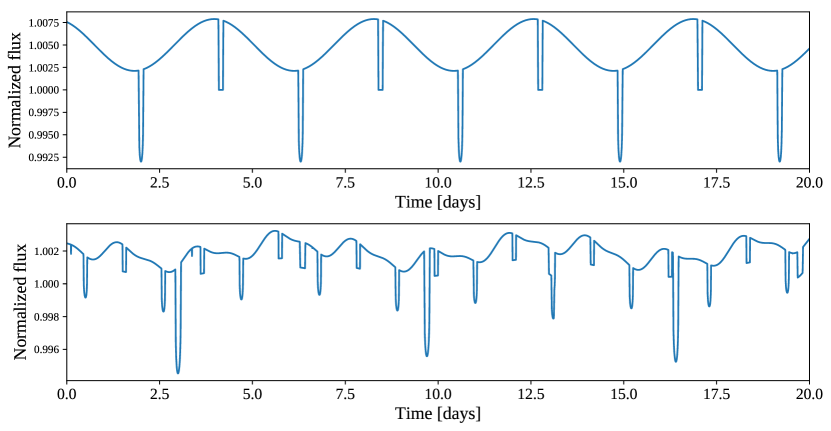
The bottom panel of the figure shows a two-planet system with more elaborate surface maps. In addition to the transits, eclipses, and complex phase curve morphology, several planet-planet occultations are also visible in the light curve.

4.6 Gradients of the light curves

Since all expressions derived in this paper are analytic, so too are their derivatives. The ability to compute derivatives of a light curve model with respect to the model parameters can be extremely useful in both optimization and inference problems. When fitting a model to data with an optimization algorithm, knowledge of the gradient of the objective function can greatly speed up convergence, as the optimizer always “knows” which direction to take a step in to improve the fit. Gradients can also be used in Hamiltonian Monte Carlo (HMC) simulations, in which the gradient of the likelihood is used to improve the efficiency of the sampler and greatly speed up convergence of the chains (e.g., Betancourt, 2017).

In principle, one could differentiate the recurrence relations in the Appendix and arrive at expressions for the derivatives of a light curve with respect to any of the input parameters. Pál (2008) derived gradients in this fashion for the case of transits across a quadratically limb-darkened star. However, for the complex surface maps we consider here, differentiating all our equations would be an extremely tedious task. Instead, we can take advantage of the analytic nature of our expressions and compute all derivatives using automatic differentiation (autodiff; e.g., Wengert, 1964). Despite the complexity of the expressions we derive here, each of the individual steps involved in computing a light curve is either a basic arithmetic operation or the evaluation of an elementary function and is therefore trivially differentiable. Autodiff algorithms exploit this fact by repeatedly applying the chain rule to compute the derivatives of any function during its evaluation, returning derivatives that can be accurate to high precision and at a speed that can be significantly greater than that of numeric (or symbolic) differentiation.

We employ the autodiff algorithm of the Eigen (Guennebaud et al., 2010) C++ library to compute derivatives of the flux with respect to all input parameters. Although fast, evaluation of the derivatives introduces overhead to the computation and is therefore disabled by default. To enable it, users should pass the gradient=True keyword argument to Map.flux() or kepler.System.compute(). In the former case, the gradient is returned in a tuple alongside the flux; in the latter, the gradient of the total light curve is stored in the gradient property of the system, and the gradient of each body’s light curve is stored in that body’s own gradient property. As an example, let us instantiate a Map class and compute the flux at one point during an occultation:

⬇

19map = Map(lmax=1)

20map[1, 0] = 0.5

21flux, gradient = map.flux(theta=30, xo=0.1, yo=0.1, ro=0.1,

22 gradient=True)

Running the code above returns the value of the flux, 1.48216…, as well as a dictionary of derivatives of the flux with respect to all input parameters:

⬇

5{'theta': array([-0.0049768]),

6 'xo': array([-0.00356856]),

7 'yo': array([0.00076157]),

8 'ro': array([-0.35638527]),

9 'y': array([[ 0.99 ],

10 [-0.00173205],

11 [ 0.98432307],

12 [-0.57029919]]),

13 'u': array([])}

These are the derivatives with respect to the rotational phase, the position and radius of the occultor, and each of the spherical harmonic and limb darkening coefficients.

Figure 10: Transit (top left) and secondary eclipse (top right) of a mildly eccentric, slightly inclined, quickly-rotating hot Jupiter with a dipole map, computed with starry. Derivatives as a function of time for several of these parameters are plotted in orange below each light curve. Solid lines correspond to the analytic derivatives and dots correspond to derivatives evaluated numerically using finite differences. From top to bottom, the curves correspond to derivatives with respect to time, planet radius, planet luminosity, orbital period, eccentricity, inclination, longitude of pericenter, rotational period, five of the planet surface map coefficients, and the linear and quadratic stellar limb darkening coefficients.   

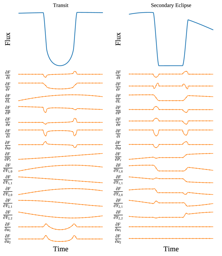
Figure 10 shows an example of the autodiff capabilities of starry for a transit and a secondary eclipse of a hot Jupiter.

4.7 Benchmarks

We validate all our calculations of rotational phase curves and occultation light curves by comparing them to numerical solutions of the corresponding surface integrals. We integrate the specific intensity of the body by discretely summing over its surface map on an adaptive radial mesh whose resolution is iteratively increased wherever the spatial gradient of the specific intensity is large and in the vicinity of the limb of the occultor.

All light curves in Figure 5 show the flux computed in this way as the small points along each of the curves. We find that our analytic light curves agree with the numerical solutions to within the error of the latter, which is on the order of $10^{-5}$.

Figure 11: Error in the terms of the solution vector $\mathbf{s}$ for a small occultor ($r=0.01$, left) and a large occultor ($r=100$, right), computed relative to calculations using quadruple floating point precision. The error is plotted as a function of impact parameter for terms with $\mu$ even (left) and $\mu$ odd (right). The horizontal axis extends from $0$ to $r+1$ (left panel) $r-1$ to $r+1$ (right panel) and covers the entire range of $b$ during an occultation, with extra resolution near potentially unstable regions. The top panel shows the relative error and the bottom panel shows the fractional error, scaled to the largest value of $\mathbf{s}$ over the course of the occultation.   

Figure 12: Similar to Figure 11, but showing instead the error on the derivative of the flux with respect to the impact parameter computed analytically with autodifferentiation. The error is computed relative to a numerical derivative computed at 128 bit precision.   

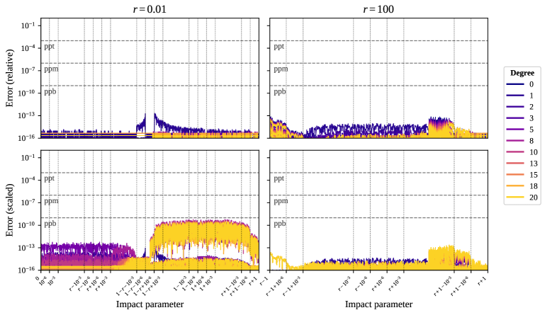
To test for numerical stability, we also compare our calculations to the same calculations performed at quadruple (128-bit) floating-point precision. Figure 11 shows the relative error on the computation of each of the terms in the solution vector $\mathbf{s}$ up to $l=20$ for a small occultor (left) and a large occultor (right). The horizontal axis corresponds to the impact parameter, spanning all possible values of $b$ during an occultation. In both cases, the maximum relative error (top panel) is less than one part per trillion. The bottom panel shows the fractional error, equal to the relative error scaled to the largest value of the function during the occultation. In cases where the largest value of the flux is less than $10^{-9}$, we scale the relative error to this value to avoid division by a very small number. In all cases, the fractional error is less than 1 ppb.

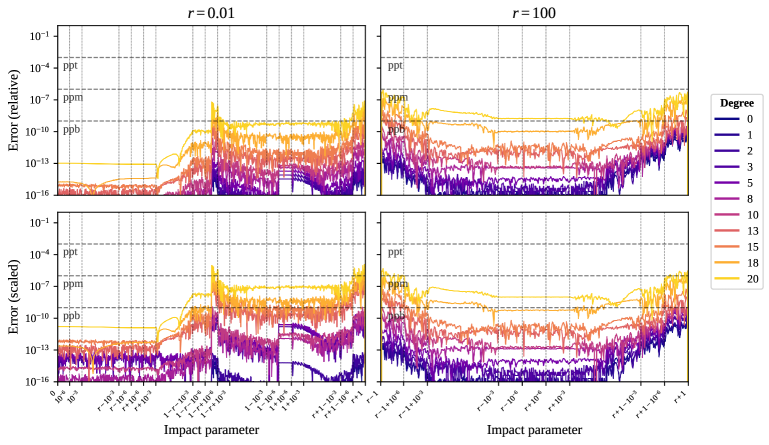
In Figure 12 we show similar curves for the numerical error on the derivative of the flux with respect to the impact parameter. While the derivatives are in general more prone to numerical instabilities, particularly in the limits $b\rightarrow|1-r|$ and $b\rightarrow 1+r$, we find that the error is less than 1 ppb over most of the domain for both small and large occultors. For large values of $l$ near the unstable regions, the error approaches 1 ppm.

Figure 13: Secondary eclipse ingress for the Earth being occulted by the Sun ($r=110$), computed for a $l=20$ expansion of the planet’s surface map. The relative error due to floating point precision loss is shown at the bottom and is less than one part per billion everywhere.   

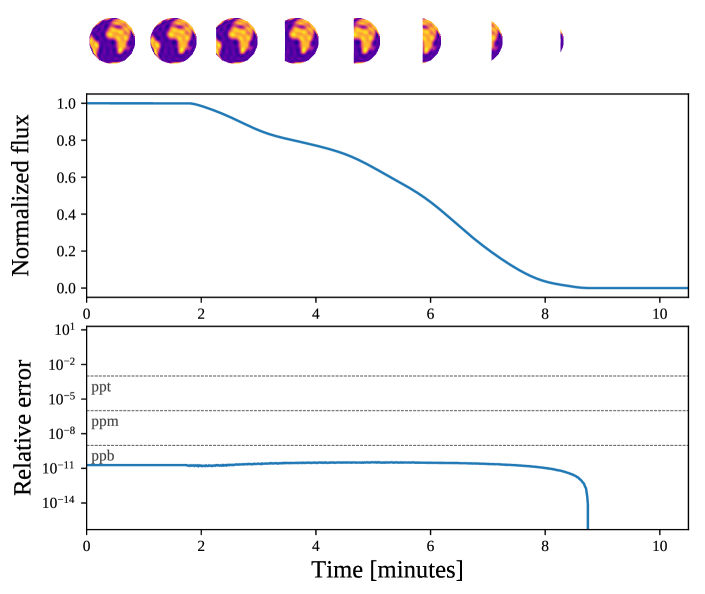
Figure 13 shows the error on a secondary eclipse light curve for an $l=20$ expansion of the Earth being occulted by the Sun. As expected, the relative error (relative to the Earth’s flux) is much less than 1 part per billion everywhere.

Figure 14: Comparison to a light curve generated using the spiderman code (Louden & Kreidberg, 2018). The top panel shows a secondary eclipse of a hot Jupiter with an offset dipole computed with starry (solid grey) and spiderman (dashed blue), and the bottom panel shows the absolute value of the difference between the two light curves as the number of layers in the spiderman grid is increased. The spiderman solution slowly approaches the starry solution as the number of layers is increased.   

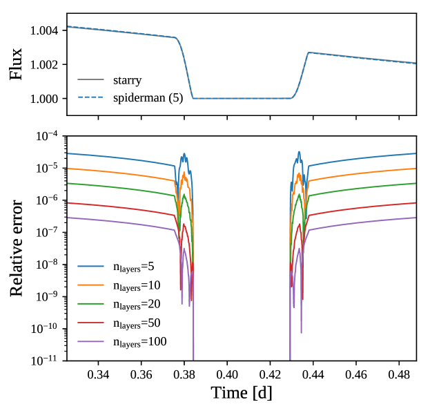
Finally, we compare our secondary eclipse and phase curve computations to light curves generated using the spiderman package (Louden & Kreidberg, 2018). The top panel of Figure 14 shows a secondary eclipse light curve for a hot Jupiter with an offset dipole map ($l=1$) computed with starry (solid blue) and spiderman (dashed orange) using the default number of layers ($n_{\mathrm{layers}}=5$) in their discretized surface intensity grid. The bottom panel shows the relative difference between the spiderman flux and the starry flux for different values of $n_{\mathrm{layers}}$. For the default number of layers, the maximum relative error in the spiderman flux is on the order of 30 ppm (relative to the stellar flux) during ingress and egress and is somewhat higher at the peak of the phase curve. Relative to the planet flux, the error is more significant: $\sim 30/0.004=7500$ ppm. This error decreases linearly as the number of layers increases, and the spiderman solution appears to approach the starry solution in the limit $n_{\mathrm{layers}}\rightarrow\infty$.

4.8 Speed tests

Figure 15 shows the evaluation time for occultation calculations as a function of the spherical harmonic degree $l$ of the map. Analytic solutions computed with starry are shown as the blue dots (purple dots for solutions with gradients enabled). Also shown are calculations using the adaptive mesh technique described in the previous section (orange dots), brute-force integration on a 300$\times$300 Cartesian grid (green dots), and numerical evaluation of the double integral using the scipy.integrate.dblquad (Jones et al., 2001) routine (red). The size of each point is proportional to the log of the fractional error relative to the starry quadruple floating-point precision solution. Light curve computation using starry is several orders of magnitude faster and more accurate than any other evaluation technique.

Figure 15: Evaluation time for a single occultation calculation as a function of the spherical harmonic degree of the map using starry (blue), starry with gradients (purple), the adaptive mesh technique (§4.7, orange), brute force integration on a Cartesian grid (green), and scipy’s dblquad two-dimensional numerical integration routine (red). The size of each point is proportional to the log of the error relative to the starry quadruple-precision solution.   

Figure 16: Speed tests for starry, showing the light curve evaluation time as a function of number of light curve points for rotational phase curves (left) and occultation light curves (right) of individual spherical harmonics. The top panels show the evaluation time for spherical harmonics of different degrees $l$, averaged over all orders $m$. The bottom panels show the time for each of the non-negative orders ($m\geq 0$) of the $l=5$ harmonics.   

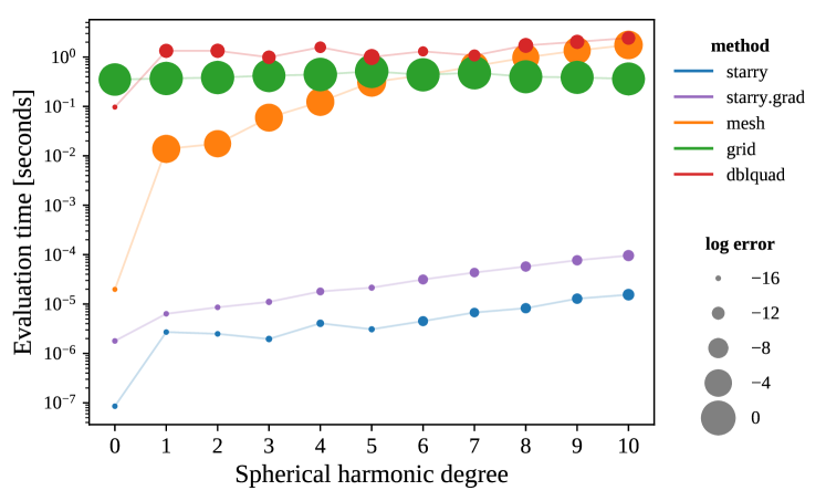
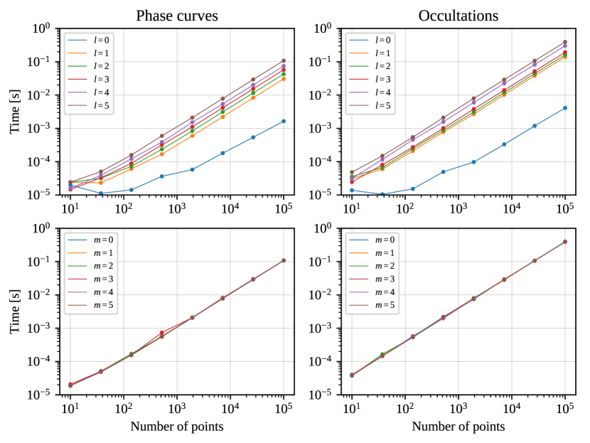
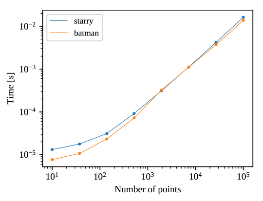
Figure 16 shows the evaluation time for starry as a function of the number of points in the light curve for phase curves (left) and occultation light curves (right). The top panel shows curves for maps of different degree $l$, and the bottom panel shows curves for single-order maps of degree $l=5$. Evaluation time scales exponentially with increasing degree, but starry can compute full occultation light curves for $l=5$ maps with $10^{5}$ points in under one second. Evaluation time is roughly constant across the different orders at fixed degree. In Figure 17 we show a speed comparison to the batman transit package (Kreidberg, 2015) for transits across a quadratically limb-darkened star. starry is as efficient as batman at computing transit light curves.

Figure 17: Speed comparison to the batman transit modeling package (Kreidberg, 2015) for a hot Jupiter transit across a quadratically limb-darkened star.   

Figure 18: Speed comparison to the spiderman code package (Louden & Kreidberg, 2018). For a dipole ($l=1$) map, starry computes secondary eclipse light curves and phase curves in about an order of magnitude less time compared to spiderman with 5 layers in their surface intensity grid. The size of the markers is proportional to the log of the error in the solutions, compared to evaluation of the equations presented in this paper using quadruple floating-point precision. As the number of layers is increased in spiderman, the error decreases linearly, but the evaluation time increases proportionally.   

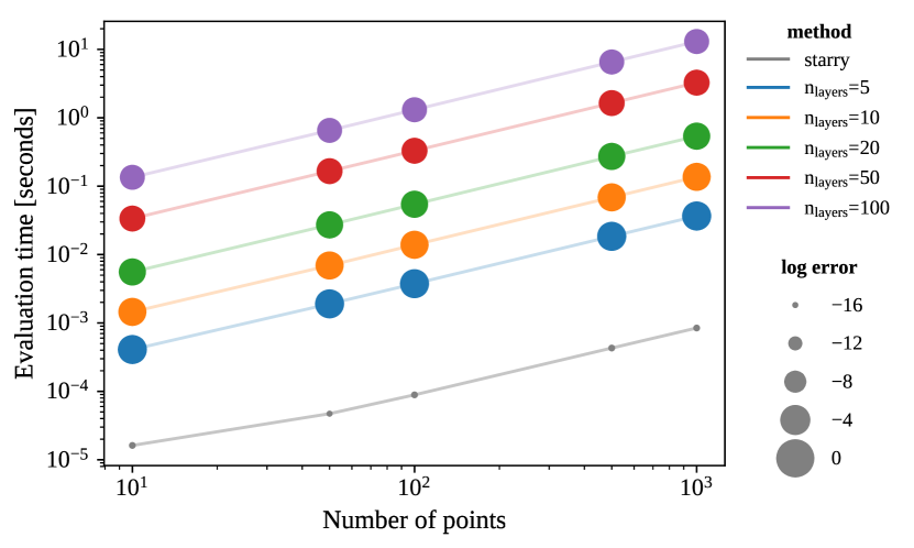
Finally, Figure 18 shows the evaluation time for starry compared to that for spiderman (Louden & Kreidberg, 2018) for a secondary eclipse of a simple $l=1$ map and varying values of the number of layers in the spiderman grid. The size of the points is proportional to the log of the relative error on the solution (see Figure 14). The evaluation time for starry is about one order of magnitude less than spiderman for the default $n_{\mathrm{layers}}=5$, for which the error is about 30 ppm (relative to the stellar flux). Computation of the spiderman light curves with larger values of $n_{\mathrm{layers}}$ improves the precision but leads to proportionally longer evaluation times.

4.9 Application to real data: HD 189733b

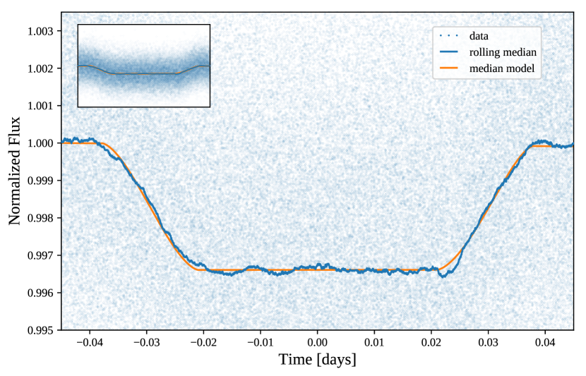
As a brief example of the application of starry to a real dataset, we analyzed the well-studied Spitzer/IRAC 8 $\mu$m secondary eclipse light curve of the hot jupiter HD 189733b from Knutson et al. (2007). Our analysis is very similar to that of Majeau et al. (2012), who also fit a spherical harmonic map to the secondary eclipse data, but evaluated their model numerically. We fit for the $l=1$ map coefficients and the planet luminosity, holding the orbital parameters constant for simplicity. Unlike Majeau et al. (2012), we fit each of the nearly 128,000 observations in the timeseries without binning. We first find the maximum likelihood fit to the data using gradient-descent optimization, then initialize an MCMC sampler in a Gaussian ball about this solution and run a chain of 40 walkers for 10,000 steps using the emcee package (Foreman-Mackey et al., 2013). At a rate of about one million flux evaluations per second, the full calculation took on the order of 10 CPU hours. Note that this is almost certainly overkill; given the extremely low signal-to-noise ratio of each measurement, binning the dataset in time could allow for runtimes of less than one hour that would yield virtually the same results.

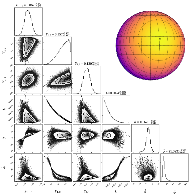
Figure 19 shows the secondary eclipse light curve and our median model fit to the data. Figure 20 shows the marginalized posteriors and covariances of our four model parameters, as well as the latitude ($\hat{\phi}$) and longitude ($\hat{\theta}$) of the hotspot relative to the substellar point. A map corresponding to the maximum likelihood model is plotted at the top right, showing a statistically significant eastward offset in the location of the hotspot in agreement with previous studies (Knutson et al., 2007; Majeau et al., 2012; de Wit et al., 2012). There is also evidence for a slight northward offset, although it is less statistically significant and consistent with zero. Note that because we did not simultaneously fit phasecurve data, there is a strong degeneracy between the planet’s total luminosity and the $Y_{1,0}$ spherical harmonic coefficient. Moreover, since we did not account for the uncertainty in the planet’s orbital parameters, we are likely underestimating the uncertainty on the map coefficients.

Figure 19: Secondary eclipse light curve of HD 189733b observed with Spitzer/IRAC at 8 $\mu$m from Knutson et al. (2007) along with our fit to the data. The inset at the top left shows a zoomed-out version of the timeseries.   

Figure 20: Posterior distributions of our model parameters from the fit to the HD189733b secondary eclipse, plotted using the corner package (Foreman-Mackey, 2016). We fit for the spherical harmonic coefficients $Y_{1,-1}$, $Y_{1,0}$, and $Y_{1,1}$, as well as the planet luminosity $L$. The latitude $\hat{\phi}$ and longitude $\hat{\theta}$ of the hotspot were calculated from these coefficients. The median value of each parameter was used to generate the map of HD189733b shown in the upper right. An X marks the inferred location of the hotspot and contour levels indicate 10% drops in specific intensity. For reference, a latitude/longitude grid is superimposed with cells measuring $15^{\circ}$ on a side.   

5 Caveats

5.1 Wavelength dependence

In our formalism thus far we have avoided mention of wavelength dependence of a body’s surface map. In our derivations we treated the specific intensity at a point on the body’s map as a scalar: a single number corresponding to the total power emitted to space by an infinitesimal area element on the body’s surface. When applying starry to actual data, this intensity can either be the power integrated over a range of wavelengths, in which case the light curve has units of flux proper, corresponding to (say) the quantity measured by an instrument performing filter photometry; or the power at a specific wavelength, in which case the light curve computed by starry has units of spectral flux, corresponding to (say) the flux measured in a tiny wavelength bin by a spectrometer. Note, importantly, that in the former case the “surface map” is in reality the integral of the body’s wavelength-dependent specific intensity convolved with the instrument’s spectral response function over a given wavelength range.

Alternatively, inspection of Equation ((LABEL:starry)) suggests that the methods outlined above for computing light curves can be trivially extended to wavelength-dependent maps. Since neither the solution vector, the change of basis matrix, nor the rotation matrices depend on the values of the map coefficients, one can compute a wavelength-dependent light curve as

$${\mathbf{f}}={\mathbf{s}}^{\boldsymbol{\mathsf{T}}}{\mathbf{A}}\,{\mathbf{R^{\prime}}}\,{\mathbf{R}}\,{\mathbf{Y}}\hskip 0.0pt,$$ (41)

where ${\mathbf{f}}$ is the vector of fluxes, one per wavelength bin, and ${\mathbf{Y}}$ is now a matrix of spherical harmonic coefficients, where each column is the usual ${\mathbf{y}}$ vector corresponding to a specific wavelength bin. This method makes it extremely fast to compute wavelength-dependent light curves, since the solution vector and rotation matrices need only be computed once for all wavelength bins.

In starry, users can set the nwav keyword argument when instantiating maps to indicate the number of wavelength bins (the default is 1). For multi-wavelength maps, the coefficient at a given value of (l, m) is a vector, corresponding to the value of the spherical harmonic coefficient in each wavelength bin. All intensities, fluxes, and gradients computed by starry gain an extra dimension in this case.

5.2 Reflectance light curves

At present, starry can only compute thermal phase curves and occultation light curves for planets and moons. Reflectance light curves are significantly more difficult to compute analytically because of the sharp discontinuity in the illumination gradient at the terminator. In principle, the stellar illumination pattern could be modeled with a high order spherical harmonic expansion, but this approach cannot accurately capture the sharp day/night transition at the terminator and typically leads to spurious ringing on the night side. A better approach is to treat the terminator as one of the boundaries of the surface integral and use Green’s theorem to compute the line integral about this elliptical curve. This will be the topic of a future paper and will be implemented in future versions of the code.

5.3 Anisotropic emission

It is important to note that the formalism developed here for computing light curves (excepting our treatment of limb darkening) implicitly assumes isotropic emission from the body’s surface. While this is usually an appropriate assumption for emission, it could break down due to scattering by, say, clouds or hazes in a planet’s atmosphere.

5.4 Physical surface maps

While spherical harmonics are a convenient way to approximate surface maps of celestial bodies, it is not trivial to ensure that a given spherical harmonic expansion ${\mathbf{y}}$ evaluates to non-negative values everywhere on the unit sphere. This is because there is no analytic way to compute the extrema of a function of spherical harmonics of arbitrary degree. This fact makes it difficult to enforce the physical prior that the specific intensity of a celestial body cannot be negative, which could be desirable when fitting a model to real data. The minimum can, of course, be found numerically. In starry, users can check whether a map is positive semi-definite (P.S.D.) by evaluating

⬇

22map.is_physical()

which returns either True (the map is non-negative everywhere) or False (at least one region on the map has a negative specific intensity). This method evaluates the surface map on a coarse grid in $\uptheta$ and $\upphi$, locates the approximate location of the minimum, and performs a gradient-descent optimization to locate the global minimum of the map.

Note that if any limb darkening coefficients are set, this method will separately determine whether the limb darkening profile is physical by ensuring that it is positive everywhere and monotonically decreasing toward the limb.

5.5 Maps of very large degree

For very large values of the spherical harmonic degree $l$, the equations presented here may become numerically unstable. The evaluation of the spherical harmonics depends on ratios of several factorials, whose precision can degrade for large $l$ and $m$. Similarly, the coefficients of the occultation solution vector $\mathbf{s}$ can drop below machine precision at large $l$, leading to further numerical issues. While starry is specifically coded up to minimize numerical instabilities, we find that for $l_{\mathrm{max}}\geq 30$ numerical issues may occur. Fortunately, situations in which maps of such high degree are necessary are not likely for exoplanet science in the foreseeable future. Nevertheless, if users wish to perform calculations for very large $l$, they can avoid these numerical issues by instantiating a multi-precision map:

⬇

13map = Map(multi=True)

By default, this will perform all calculations using quadruple (128-bit) floating point precision. We caution, however, that this will increase computation time by at least an order of magnitude.

5.6 Three-body events

The occultation formalism developed in this paper applies specifically to the case of a single occultor, so starry cannot at present handle mutual occultations involving more than two bodies; if a three-body event occurs, the computed flux will be incorrect. However, even for an arbitrary number of bodies the problem is still analytic, since Green’s theorem may be employed in the same way, but instead evaluating the line integrals along the more complex network of arcs defining the edges of the visible portion of the body’s surface. This was first noted by Pál (2012), whose mttr code computes analytic transit light curves for mutually overlapping bodies such as a transiting planet with a moon. Future versions of starry will extend the calculations to this general case.

6 Conclusions

In this paper, we derived a formalism to compute analytic thermal light curves of celestial bodies in occultation, provided their specific intensity maps can be expressed as a sum of spherical harmonics. Our expressions extend the analytic results of the Mandel & Agol (2002) transit model for limb-darkened stars to transits and occultations of celestial bodies whose surface maps are not radially symmetric and/or possess higher order features, and are thus generally applicable to stars, planets, and moons. We derived recurrence relations to quickly compute occultation light curves for surface maps expressed at arbitrary spherical harmonic degree. We showed, in particular, that the flux contribution from higher degree terms depends on the same elliptic integrals as the linear limb darkening term, so these need only be evaluated once per light curve cadence. This results in evaluation times for higher degree maps that are extremely fast, and only marginally slower than in the quadratic limb darkening case. In the limit of zero occultor size, our expressions trivially reduce to equations for thermal phase curves of celestial bodies.

We introduced starry, a Python-wrapped model coded in C++ that can be used to compute phase curves and occultation light curves for individual celestial bodies or entire exoplanet systems. starry computes transits, secondary eclipses, phase curves, and planet-planet occultations analytically and is comparable in speed to other transit-modeling packages such as batman (Kreidberg, 2015). Because the light curves are all analytic, starry can also easily compute analytic gradients of the light curves with respect to all input parameters via autodifferentiation, facilitating its interface with gradient-based inference schemes such as Hamiltonian Monte Carlo (HMC) or gradient-descent optimization methods.

Although we have in mind the application of this starry to exoplanets, it could in principle be applied to eclipsing binaries as well. If the deformation of the body is small and reflection is negligible, as is the case for long orbital periods, then the surface brightness of each star can be decomposed into spherical harmonics, and the starry formalism may be used to integrate their phase curves and eclipses. One could imagine applying starry, for instance, to secondary eclipses of white dwarfs to search for non-uniform surface brightness.

At present, starry supports only monochromatic surface maps, making it ideally suited for the modeling of light curves collected via filter photometry, but future work will extend it to spectrophotometry. starry is also limited to thermal light curves of planets and moons, since the discontinuity in the gradient of the illumination pattern at the terminator makes it more challenging to analytically solve the surface integrals in reflected light. However, an analytic solution is likely to exist, and future work aims to extend starry to this case.

The upcoming James Webb Space Telescope (JWST) and eventual next-generation telescopes such as the Origins Space Telescope (OST) will measure exoplanet secondary eclipses and phase curves in the thermal infrared to unprecedented precision. starry can compute extremely fast and high-precision models for these light curves, enabling the reconstruction of two-dimensional maps of these alien worlds.

Appendix A Spherical harmonics

In spherical coordinates, the spherical harmonics may be compactly represented as in Equation (1). The formalism in this paper requires us to express them in Cartesian form, which is somewhat more cumbersome but still tractable. Using Equation (2.1) and expanding Equation (1) via the multiple angle formula, we obtain

$$Y_{lm}(\mbox{$x$},\mbox{$y$},\mbox{$z$})=\left(\frac{1}{\sqrt{1-\mbox{$z$}^{2}}}\right)^{|m|}\begin{dcases}\bar{P}_{lm}(\mbox{$z$})\sum_{j\,\mathrm{even}}^{m}\left(-1\right)^{\frac{j}{2}}\binom{m}{j}\mbox{$x$}^{m-j}\mbox{$y$}^{j}&\qquad m\geq 0\\[10.00002pt] \bar{P}_{l|m|}(\mbox{$z$})\sum_{j\,\mathrm{odd}}^{|m|}\left(-1\right)^{\frac{j-1}{2}}\binom{|m|}{j}\mbox{$x$}^{|m|-j}\mbox{$y$}^{j}&\qquad m<0\hskip 0.0pt,\end{dcases}$$ (A1)

where $\binom{\scaleto{\cdot}{6pt}}{\scaleto{\cdot}{6pt}}$ is the binomial coefficient. The normalized associated Legendre functions are defined as

$$\bar{P}_{lm}(\mbox{$z$}) =A_{lm}\left(\sqrt{1-\mbox{$z$}^{2}}\right)^{m}\frac{\mathrm{d}^{m}}{\mathrm{d}\mbox{$z$}^{m}}\left[\frac{1}{2^{l}l!}\frac{\mathrm{d}^{l}}{\mathrm{d}\mbox{$z$}^{l}}\left(\mbox{$z$}^{2}-1\right)^{l}\right]\hskip 0.0pt,$$ (A2)

where

$$A_{lm}=\sqrt{\frac{(2-\delta_{m0})(2l+1)(l-m)!}{4\pi(l+m)!}}\hskip 0.0pt.$$ (A3)

Expanding out the $z$ derivatives, we obtain

$$\bar{P}_{lm}(\mbox{$z$}) =A_{lm}\left(\sqrt{1-\mbox{$z$}^{2}}\right)^{m}\sum_{k=0}^{l-m}\frac{2^{l}\left(\frac{l+m+k-1}{2}\right)!}{k!(l-m-k)!\left(\frac{-l+m+k-1}{2}\right)!}\mbox{$z$}^{k}\hskip 0.0pt,$$ (A4)

which we combine with the previous results to write

$$Y_{lm}(\mbox{$x$},\mbox{$y$},\mbox{$z$}) =\begin{dcases}\sum_{j\,\mathrm{even}}^{m}\sum_{k=0}^{l-m}\left(-1\right)^{\frac{j}{2}}A_{lm}B_{lm}^{jk}\mbox{$x$}^{m-j}\mbox{$y$}^{j}\mbox{$z$}^{k}\qquad&m\geq 0\\ \sum_{j\,\mathrm{odd}}^{|m|}\sum_{k=0}^{l-|m|}\left(-1\right)^{\frac{j-1}{2}}A_{l|m|}B_{l|m|}^{jk}\mbox{$x$}^{|m|-j}\mbox{$y$}^{j}\mbox{$z$}^{k}\qquad&m<0\end{dcases}$$  (A5)

where

$$B_{lm}^{jk}=\frac{2^{l}m!\left(\frac{l+m+k-1}{2}\right)!}{j!k!(m-j)!(l-m-k)!\left(\frac{-l+m+k-1}{2}\right)!}\hskip 0.0pt.$$ (A6)

Since we are confined to the surface of the unit sphere, we have $\mbox{$z$}=\sqrt{1-\mbox{$x$}^{2}-\mbox{$y$}^{2}}$ and we may expand $\mbox{$z$}^{k}$ using the binomial theorem:

$$\mbox{$z$}^{k} =(1-\mbox{$x$}^{2}-\mbox{$y$}^{2})^{\frac{k}{2}}$$

$$=\begin{dcases}\sum_{p\,\mathrm{even}}^{k}\sum_{q\,\mathrm{even}}^{p}(-1)^{\frac{p}{2}}C_{pq}^{k}\mbox{$x$}^{p-q}\mbox{$y$}^{q}\qquad&k\,\mathrm{even}\\ \sum_{p\,\mathrm{even}}^{k-1}\sum_{q\,\mathrm{even}}^{p}(-1)^{\frac{p}{2}}C_{pq}^{k-1}\mbox{$x$}^{p-q}\mbox{$y$}^{q}\sqrt{1-\mbox{$x$}^{2}-\mbox{$y$}^{2}}\qquad&k\,\mathrm{odd}\hskip 0.0pt,\end{dcases}$$ (A7)

where

$$C_{pq}^{k}=\frac{\left(\frac{k}{2}\right)!}{\left(\frac{q}{2}\right)!\left(\frac{k-p}{2}\right)!\left(\frac{p-q}{2}\right)!}\hskip 0.0pt.$$ (A8)

This gives us an expression for the spherical harmonics $Y_{lm}$ as a function of $x$ and $y$ only:

$$Y_{lm}(\mbox{$x$},\mbox{$y$}) =\begin{dcases}\!\begin{aligned} &\sum_{j\,\mathrm{even}}^{m}\sum_{k\,\mathrm{even}}^{l-m}\sum_{p\,\mathrm{even}}^{k}\sum_{q\,\mathrm{even}}^{p}\left(-1\right)^{\frac{j+p}{2}}A_{lm}B_{lm}^{jk}C_{pq}^{k}\mbox{$x$}^{m-j+p-q}\mbox{$y$}^{j+q}\,+\\ &\sum_{j\,\mathrm{even}}^{m}\sum_{k\,\mathrm{odd}}^{l-m}\sum_{p\,\mathrm{even}}^{k-1}\sum_{q\,\mathrm{even}}^{p}\left(-1\right)^{\frac{j+p}{2}}A_{lm}B_{lm}^{jk}C_{pq}^{k-1}\mbox{$x$}^{m-j+p-q}\mbox{$y$}^{j+q}\mbox{$z$}\end{aligned}&\hskip 0.0ptm\geq 0\\ \\ \!\begin{aligned} &\sum_{j\,\mathrm{odd}}^{|m|}\sum_{k\,\mathrm{even}}^{l-|m|}\sum_{p\,\mathrm{even}}^{k}\sum_{q\,\mathrm{even}}^{p}\left(-1\right)^{\frac{j+p-1}{2}}A_{l|m|}B_{l|m|}^{jk}C_{pq}^{k}\mbox{$x$}^{|m|-j+p-q}\mbox{$y$}^{j+q}\,+\\ &\sum_{j\,\mathrm{odd}}^{|m|}\sum_{k\,\mathrm{odd}}^{l-|m|}\sum_{p\,\mathrm{even}}^{k-1}\sum_{q\,\mathrm{even}}^{p}\left(-1\right)^{\frac{j+p-1}{2}}A_{l|m|}B_{l|m|}^{jk}C_{pq}^{k-1}\mbox{$x$}^{|m|-j+p-q}\mbox{$y$}^{j+q}\mbox{$z$}\end{aligned}&\hskip 0.0ptm<0\end{dcases}$$  (A9)

where $\mbox{$z$}=\mbox{$z$}(\mbox{$x$},\mbox{$y$})=\sqrt{1-\mbox{$x$}^{2}-\mbox{$y$}^{2}}$. Evaluating the nested sums may be computationally slow, but these operations need only be performed a single time to construct our change of basis matrix (following section).

Appendix B Change of Basis

In this section we discuss how to compute the change of basis matrices ${\mathbf{A_{1}}}$ and ${\mathbf{A_{2}}}$ from §2.3 and provide links to Jupyter scripts to compute them. Recall that the columns of the change of basis matrix from spherical harmonics to polynomials, ${\mathbf{A_{1}}}$, are just the polynomial vectors corresponding to each of the spherical harmonics in Equation ((LABEL:by)). From Equations (7) and (A9), we can calculate the first few spherical harmonics and their corresponding polynomial vectors:

$$\begin{array}[]{@{}lcccccccl@{}}\phantom{..}Y_{0,0}=\frac{1}{2\sqrt{\pi}}&&&&&&&&{\mathbf{p}}=\frac{1}{2\sqrt{\pi}}\begin{pmatrix}1&0&0&0&\cdot\cdot\cdot\end{pmatrix}^{\mathsf{T}}\\ Y_{1,-1}=\frac{\sqrt{3}}{2\sqrt{\pi}}\mbox{$y$}&&&&&&&&{\mathbf{p}}=\frac{1}{2\sqrt{\pi}}\begin{pmatrix}0&0&0&\sqrt{3}&\cdot\cdot\cdot\end{pmatrix}^{\mathsf{T}}\\ \phantom{..}Y_{1,0}=\frac{\sqrt{3}}{2\sqrt{\pi}}\mbox{$z$}&&&&&&&&{\mathbf{p}}=\frac{1}{2\sqrt{\pi}}\begin{pmatrix}0&0&\sqrt{3}&0&\cdot\cdot\cdot\end{pmatrix}^{\mathsf{T}}\\ \phantom{..}Y_{1,1}=\frac{\sqrt{3}}{2\sqrt{\pi}}\mbox{$x$}&&&&&&&&{\mathbf{p}}=\frac{1}{2\sqrt{\pi}}\begin{pmatrix}0&\sqrt{3}&0&0&\cdot\cdot\cdot\end{pmatrix}^{\mathsf{T}}\\ Y_{2,-2}=\cdot\cdot\cdot&&&&&&&&{\mathbf{p}}=\cdot\cdot\cdot\end{array}$$ (B1)

From these we can construct ${\mathbf{A_{1}}}$. As an example, for spherical harmonics up to degree $l_{\mathrm{max}}=2$, this is

$$\setstackgap{L}{1.25}\fixTABwidth{T}{\mathbf{A_{1}}}=\frac{1}{2\sqrt{\pi}}\parenMatrixstack{1&00000\sqrt{5}00\\ 000\sqrt{3}00000\\ 00\sqrt{3}000000\\ 0\sqrt{3}0000000\\ 000000-\frac{3\sqrt{5}}{2}0\frac{\sqrt{15}}{2}\\ 0000000\sqrt{15}0\\ 0000\sqrt{15}0000\\ 00000\sqrt{15}000\\ 000000-\frac{3\sqrt{5}}{2}0-\frac{\sqrt{15}}{2}}\hskip 0.0pt.$$  (B2)

We compute the change of basis matrix from polynomials to Green’s polynomials, ${\mathbf{A_{2}}}$, in a similar manner. In practice, it is easier to express the elements of the Green’s basis $\tilde{{\mathbf{g}}}$ in terms of the elements of the polynomial basis $\tilde{{\mathbf{p}}}$ and use those to populate the columns of the matrix ${\mathbf{A_{2}}}^{-1}$. Continuing our example for $l_{\mathrm{max}}=2$, our second change of basis matrix is

$$\setstackgap{L}{1.1}\fixTABwidth{T}{\mathbf{A_{2}}}=\parenMatrixstack{\hskip 0.0pt\hskip 0.0pt\,1\,\hskip 0.0pt\hskip 0.0pt\hskip 0.0pt\hskip 0.0pt&00000000\\ 0\frac{1}{2}0000000\\ 001000000\\ 000100000\\ 0000\frac{1}{3}0000\\ 00000-\frac{1}{3}000\\ 000000\frac{1}{2}00\\ 0000000\frac{1}{3}0\\ 000000001}\hskip 0.0pt.$$  (B3)

Finally, recall that the complete change of basis matrix from spherical harmonics to Green’s polynomials, ${\mathbf{A}}$, is just the matrix product of ${\mathbf{A_{2}}}$ and ${\mathbf{A_{1}}}$. For $l_{\mathrm{max}}=2$, we have

$$\setstackgap{L}{1.25}\fixTABwidth{T}{\mathbf{A}}=\frac{1}{2\sqrt{\pi}}\parenMatrixstack{1&00000\sqrt{5}00\\ 000\frac{\sqrt{3}}{2}00000\\ 00\sqrt{3}000000\\ 0\sqrt{3}0000000\\ 000000-\frac{\sqrt{5}}{2}0\frac{\sqrt{\frac{5}{3}}}{2}\\ 0000000-\sqrt{\frac{5}{3}}0\\ 0000\frac{\sqrt{15}}{2}0000\\ 00000\sqrt{\frac{5}{3}}000\\ 000000-\frac{3\sqrt{5}}{2}0-\frac{\sqrt{15}}{2}}\hskip 0.0pt.$$  (B4)

Appendix C Rotation of spherical harmonics

C.1 Euler angles

Collado et al. (1989) derived expressions for the rotation matrices for the real spherical harmonics of a given degree $l$ from the corresponding complex rotation matrices (Steinborn & Ruedenberg, 1973):

$${\mathbf{R}}^{l}={\mathbf{U}}^{-1}{\mathbf{D}}^{l}{\mathbf{U}}$$ (C1)

where

$${\mathbf{D}}^{l}_{m,m^{\prime}} =\mathrm{e}^{-\mathbf{i}(\alpha m^{\prime}+\gamma m)}(-1)^{m^{\prime}+m}\sqrt{(l-m)!(l+m)!(l-m^{\prime})!(l+m^{\prime})!}$$

$$\phantom{=}\times\sum_{k}(-1)^{k}\frac{\cos\left(\frac{\beta}{2}\right)^{2l+m-m^{\prime}-2k}\sin\left(\frac{\beta}{2}\right)^{-m+m^{\prime}+2k}}{k!(l+m-k)!(l-m^{\prime}-k)!(m^{\prime}-m+k)!}$$  (C2)

is the $(m,m^{\prime})$ index of the rotation matrix for the complex spherical harmonics of degree $l$ and

$$\setstackgap{L}{1.25}\fixTABwidth{T}{\mathbf{U}}=\frac{1}{\sqrt{2}}\parenMatrixstack{\hskip 0.0pt\hskip 0.0pt\,\ddots\,\hskip 0.0pt\hskip 0.0pt\hskip 0.0pt\hskip 0.0pt&\mathinner{\mkern 1.0mu\raise 1.0pt\vbox{\kern 7.0pt\hbox{.}}\mkern 2.0mu\raise 4.0pt\hbox{.}\mkern 2.0mu\raise 7.0pt\hbox{.}\mkern 1.0mu}\\ \mathbf{i}1\\ \mathbf{i}1\\ \mathbf{i}1\\ \sqrt{2}\\ \mathbf{i}-1\\ -\mathbf{i}1\\ \mathbf{i}-1\\ \mathinner{\mkern 1.0mu\raise 1.0pt\vbox{\kern 7.0pt\hbox{.}}\mkern 2.0mu\raise 4.0pt\hbox{.}\mkern 2.0mu\raise 7.0pt\hbox{.}\mkern 1.0mu}\ddots}\hskip 0.0pt.$$  (C3)

describes the transformation from complex to real spherical harmonics. In Equation ((LABEL:dl)) above, $\alpha$, $\beta$, and $\gamma$ are the (proper) Euler angles for rotation in the $z{-}y{-}z$ convention. To obtain a rotation matrix for an arbitrary vector ${\mathbf{y}}$ with spherical harmonics of different orders up to $l=l_{\mathrm{max}}$, we define the block-diagonal matrix ${\mathbf{R}}$:

$$\setstackgap{L}{1.25}\fixTABwidth{T}{\mathbf{R}}=\parenMatrixstack{\hskip 0.0pt\hskip 0.0pt\,{\mathbf{R}}^{0}\,\hskip 0.0pt\hskip 0.0pt&\\ {\mathbf{R}}^{1}\\ {\mathbf{R}}^{2}\\ {\mathbf{R}}^{3}\\ \ddots}\hskip 0.0pt.$$  (C4)

Rotation of ${\mathbf{y}}$ by the Euler angles $\alpha$, $\beta$, and $\gamma$ is performed via Equation ((LABEL:rotation)) with ${\mathbf{R}}$ given by Equation ((LABEL:rblockdiag)).

C.2 Axis-angle

It is often more convenient to define a rotation by an axis ${\mathbf{u}}$ and an angle $\theta$ of rotation about that axis. Given a unit vector ${\mathbf{u}}$ and an angle $\theta$, we can find the corresponding Euler angles by comparing the 3-dimensional Cartesian rotation matrices for both systems,

$$\setstackgap{L}{1.25}\fixTABwidth{T}\mathbf{P}=\parenMatrixstack{c_{\theta}+u_{x}^{2}\left(1-c_{\theta}\right)&u_{x}u_{y}\left(1-c_{\theta}\right)-u_{z}s_{\theta}u_{x}u_{z}\left(1-c_{\theta}\right)+u_{y}s_{\theta}\\ u_{y}u_{x}\left(1-c_{\theta}\right)+u_{z}s_{\theta}c_{\theta}+u_{y}^{2}\left(1-c_{\theta}\right)u_{y}u_{z}\left(1-c_{\theta}\right)-u_{x}s_{\theta}\\ \hskip 0.0pt\,\,u_{z}u_{x}\left(1-c_{\theta}\right)-u_{y}s_{\theta}\,\,\hskip 0.0pt\,u_{z}u_{y}\left(1-c_{\theta}\right)+u_{x}s_{\theta}c_{\theta}+u_{z}^{2}\left(1-c_{\theta}\right)}$$ (C5)

for axis-angle rotations and

$$\setstackgap{L}{1.25}\fixTABwidth{T}\mathbf{Q}=\parenMatrixstack{c_{\alpha}c_{\beta}c_{\gamma}-s_{\alpha}s_{\gamma}&-c_{\gamma}s_{\alpha}-c_{\alpha}c_{\beta}s_{\gamma}c_{\alpha}s_{\beta}\\ c_{\alpha}s_{\gamma}+c_{\beta}c_{\gamma}s_{\alpha}c_{\alpha}c_{\gamma}-c_{\beta}s_{\alpha}s_{\gamma}s_{\alpha}s_{\beta}\\ -c_{\gamma}s_{\beta}s_{\beta}s_{\gamma}c_{\beta}}\hskip 0.0pt,$$ (C6)

for Euler rotations, where $c_{\scaleto{\cdot}{6pt}}\equiv\cos(\cdot)$ and $s_{\scaleto{\cdot}{6pt}}\equiv\sin(\cdot)$. Equating the two matrices gives us expressions for the Euler angles in terms of ${\mathbf{u}}$ and $\theta$:

$$\begin{matrix}\cos\alpha=\frac{P_{0,2}}{\sqrt{P_{0,2}^{2}+P_{1,2}^{2}}}&&&&\cos\beta=P_{2,2}&&&&\cos\gamma=-\frac{P_{2,0}}{\sqrt{P_{2,0}^{2}+P_{2,1}^{2}}}\\ \sin\alpha=\frac{P_{1,2}}{\sqrt{P_{0,2}^{2}+P_{1,2}^{2}}}&&&&\sin\beta=\sqrt{1-P_{2,2}^{2}}&&&&\sin\gamma=\frac{P_{2,1}}{\sqrt{P_{2,0}^{2}+P_{2,1}^{2}}}\end{matrix}\hskip 0.0pt.$$  (C7)

Thus, given a spherical harmonic vector ${\mathbf{y}}$, we can calculate how it transforms under rotation by an angle $\theta$ about an axis ${\mathbf{u}}$ by first computing the Euler angles (Equation C7) and using those to construct the spherical harmonic rotation matrix (Equation C4).

Appendix D Computing the solution vector ${s_{n}}$

Here we seek a solution to Equation ((LABEL:sn)), which gives the total flux during an occultation of the $n^{\mathrm{th}}$ term in the Green’s basis (Equation 11). The primitive integrals $\mathcal{P}$ and $\mathcal{G}$ in that equation are given by Equations (31) and (32), with ${\mathbf{G}}_{n}$ defined in Equation ((LABEL:Gn)). Note that all of the terms in Equation ((LABEL:Gn)), with the exception of the $l=1,m=0$ case, are simple polynomials in $x$, $y$, and $z$, which facilitates their integration. The $l=1,m=0$ term (corresponding to the $n=2$ term in the Green’s basis) is more difficult to integrate, but an analytic solution exists (Pál, 2012). It is, however, more convenient to note that this term corresponds to a surface map given by the polynomial $I(x,y)=\tilde{g}_{2}(x,y)=\sqrt{1-x^{2}-y^{2}}$, which is the same function used to model linear limb darkening in stars (Mandel & Agol, 2002). We therefore evaluate this term separately in Appendix D.1 below, followed by the general term in Appendix D.2.

D.1 Linear limb darkening ($n=2$, $l=1$, $m=0$)

From Mandel & Agol (2002), the total flux visible during the occultation of a body whose surface map is given by $I(x,y)=\sqrt{1-\mbox{$x$}^{2}-\mbox{$y$}^{2}}$ may be computed as

$$s_{2}=\frac{2\pi}{3}\left(1-\frac{3\Lambda}{2}-\Theta(r-b)\right)$$ (D1)

where $\Theta(\scaleto{\cdot}{6pt})$ is the Heaviside step function and

$$\Lambda =\begin{dcases}\frac{1}{9\pi\sqrt{br}}\Bigg{[}\frac{(r+b)^{2}-1}{r+b}\Big{(}-2r\,\big{(}2(r+b)^{2}+(r+b)(r-b)-3\big{)}K(k^{2})&\\ \phantom{XXXX}+3(b-r)\,\Pi\big{(}k^{2}(b+r)^{2},\,k^{2}\big{)}\Big{)}-4br(4-7r^{2}-b^{2})E(k^{2})\Bigg{]}&\qquad k^{2}<1\\[15.00002pt] \frac{2}{9\pi}\Bigg{[}\big{(}1-(r+b)^{2}\big{)}\Bigg{(}\sqrt{1-(b-r)^{2}}\,K\left(\frac{1}{k^{2}}\right)+3\left(\frac{b-r}{(b+r)\sqrt{1-(b-r)^{2}}}\right)&\\ \phantom{XX}\times\Pi\left(\frac{1}{k^{2}(b+r)^{2}},\,\frac{1}{k^{2}}\right)\Bigg{)}-\sqrt{1-(b-r)^{2}}(4-7r^{2}-b^{2})E\left(\frac{1}{k^{2}}\right)\Bigg{]}&\qquad k^{2}\geq 1\end{dcases}$$  (D2)

with

$$k^{2} =\frac{1-r^{2}-b^{2}+2br}{4br}\hskip 0.0pt.$$ (D3)

In the expressions above, $K(\scaleto{\cdot}{6pt})$, $E(\scaleto{\cdot}{6pt})$, and $\Pi(\scaleto{\cdot}{6pt},\scaleto{\cdot}{6pt})$ are the complete elliptic integrals of the first, second kind, and third kind, respectively, defined as

$$K(k^{2}) \equiv\int_{0}^{\frac{\pi}{2}}\frac{\mathrm{d}\varphi}{\sqrt{1-k^{2}\sin^{2}\varphi}}$$

$$E(k^{2}) \equiv\int_{0}^{\frac{\pi}{2}}\sqrt{1-k^{2}\sin^{2}\varphi}\,\mathrm{d}\varphi$$

$$\Pi(n,k^{2}) \equiv\int_{0}^{\frac{\pi}{2}}\frac{\mathrm{d}\varphi}{(1-n\sin^{2}\varphi)\sqrt{1-k^{2}\sin^{2}\varphi}}\hskip 0.0pt.$$ (D4)

In some cases, the expressions above can become unstable. For $r>1$, $b\approx r$, $b+r\approx 1$, and $|b-r|\approx 1$, we re-parametrize these expressions in terms of the modified elliptic integral $\mathrm{cel}(k_{c},p,a,b)$ (Bulirsch, 1969) as described in Agol & Luger (2018).

D.2 All other terms

D.2.1 Setting up the equations

We evaluate all other terms in $s_{n}$ by integrating the primitive integrals of ${\mathbf{G}}_{n}$. These are given by

$$\mathcal{P}({\mathbf{G}}_{n}) =\begin{dcases}+\int\displaylimits_{\pi-\phi}^{2\pi+\phi}(rc_{\varphi})^{\frac{\mu+2}{2}}(b+rs_{\varphi})^{\frac{\nu}{2}}rc_{\varphi}\,\mathrm{d}\varphi&\qquad\frac{\mu}{2}\,\mathrm{even}\\[10.00002pt] -\int\displaylimits_{\pi-\phi}^{2\pi+\phi}(rc_{\varphi})^{l-2}(1{-}r^{2}{-}b^{2}{-}2brs_{\varphi})^{\frac{3}{2}}rs_{\varphi}\,\mathrm{d}\varphi&\qquad\mu=1,\,l\,\mathrm{even}\\[10.00002pt] -\int\displaylimits_{\pi-\phi}^{2\pi+\phi}(rc_{\varphi})^{l-3}(b+rs_{\varphi})(1{-}r^{2}{-}b^{2}{-}2brs_{\varphi})^{\frac{3}{2}}rs_{\varphi}\,\mathrm{d}\varphi&\qquad\mu=1,\,l\neq 1,\,l\,\mathrm{odd}\\[10.00002pt] +\int\displaylimits_{\pi-\phi}^{2\pi+\phi}(rc_{\varphi})^{\frac{\mu-3}{2}}(b+rs_{\varphi})^{\frac{\nu-1}{2}}(1{-}r^{2}{-}b^{2}{-}2brs_{\varphi})^{\frac{3}{2}}rc_{\varphi}\,\mathrm{d}\varphi&\qquad\frac{\mu-1}{2}\,\mathrm{even},\,l\neq 1\\[10.00002pt] \textrm{---}\ \mathrm{(c.f.\ Appendix\ \ref{app:linearld})}&\qquad\mu=1,\,l=1\\[10.00002pt] 0&\qquad\mathrm{otherwise}\end{dcases}$$ (D5)

and

$$\mathcal{Q}({\mathbf{G}}_{n}) =\begin{dcases}+\int\displaylimits_{\pi-\lambda}^{2\pi+\lambda}c_{\varphi}^{\frac{\mu+2}{2}}s_{\varphi}^{\frac{\nu}{2}}c_{\varphi}\,\mathrm{d}\varphi&\qquad\qquad\frac{\mu}{2}\,\mathrm{even}\\[10.00002pt] \phantom{XXXXX}0&\qquad\qquad\mathrm{otherwise,}\end{dcases}$$ (D6)

where we have used the fact that the line integral of any function proportional to $z$ taken along the limb of the occulted planet (where $\mbox{$z$}=\sqrt{1-\mbox{$x$}^{2}-\mbox{$y$}^{2}}=0$) is zero.

D.2.2 The $\mathcal{Q}$ integral

We begin with the expression for $\mathcal{Q}$ (Equation D6), as this is the most straightforward. Defining the integral

$$\mathcal{H}_{u,v} =\int\displaylimits_{\pi-\lambda}^{2\pi+\lambda}c_{\varphi}^{u}s_{\varphi}^{v}\,\mathrm{d}\varphi\hskip 0.0pt,$$ (D7)

we may write

$$\mathcal{Q}({\mathbf{G}}_{n}) =\begin{dcases}\mathcal{H}_{\frac{\mu+4}{2},\frac{\nu}{2}}&\qquad\qquad\qquad\qquad\hskip 0.0pt\hskip 0.0pt\hskip 0.0pt\hskip 0.0pt\frac{\mu}{2}\,\mathrm{even}\\[10.00002pt] 0&\qquad\qquad\qquad\qquad\hskip 0.0pt\hskip 0.0pt\hskip 0.0pt\hskip 0.0pt\mathrm{otherwise}\hskip 0.0pt.\end{dcases}$$ (D8)

Pál (2012) derived simple recurrence relations for this integral:

$$\mathcal{H}_{u,v} =\begin{dcases}0&\qquad u\ \mathrm{odd}\\[5.0pt] 2\lambda+\pi&\qquad u=v=0\\[5.0pt] -2\cos\lambda&\qquad u=0,v=1\\[5.0pt] \frac{2}{u+v}(\cos\lambda)^{u-1}(\sin\lambda)^{v+1}+\frac{u-1}{u+v}\mathcal{H}_{u-2,v}&\qquad u\geq 2\\[5.0pt] -\frac{2}{u+v}(\cos\lambda)^{u+1}(\sin\lambda)^{v-1}+\frac{v-1}{u+v}\mathcal{H}_{u,v-2}&\qquad v\geq 2\hskip 0.0pt\end{dcases}$$  (D9)

D.2.3 The $\mathcal{P}$ integral

In general, the $\mathcal{P}$ integral is more difficult to evaluate because of the term to the $\nicefrac{{3}}{{2}}$ power in several of the cases. Moreover, the presence of terms proportional to powers of $b$ and $r$ and terms of order unity in several of the integrands in Equation (D5) can lead to severe numerical instabilities when either $b$ or $r$ are very large (which is typically the case for secondary eclipses of small planets) or very small (which occurs for small transiting bodies). To enforce numerical stability in all regimes, we find that is convenient to define the parameters

$$\delta=\frac{b-r}{2r}$$ (D10)

and

$$\kappa =\phi+\frac{\pi}{2}$$

$$=\cos^{-1}\left(\frac{r^{2}+b^{2}-1}{2br}\right)\hskip 0.0pt.$$ (D11)

The latter variable can be defined more simply in terms of $\sin^{2}\tfrac{\kappa}{2}=k^{2}$, or $\kappa=2\sin^{-1}k$. Note that when $r+b\leq 1$, $\phi=\pi/2$, so $\kappa=\pi$. With this transformed variable, the limits of integration of $\mathcal{P}({\mathbf{G}}_{n})$ become $\tfrac{3\pi}{2}-\kappa$ to $\tfrac{3\pi}{2}+\kappa$. Transforming $\varphi$ to $\varphi^{\prime}=\frac{1}{2}(\varphi-\tfrac{3\pi}{2})$ yields

$$\mathcal{P}({\mathbf{G}}_{n}) =\begin{dcases}2(2r)^{l+2}\int\displaylimits_{-\kappa/2}^{\kappa/2}(s_{\varphi}^{2}-s_{\varphi}^{4})^{\frac{\mu+4}{4}}(\delta+s_{\varphi}^{2})^{\frac{\nu}{2}}\,\mathrm{d}\varphi&\qquad\frac{\mu}{2}\,\mathrm{even}\\[10.00002pt] \mathcal{F}\int\displaylimits_{-\kappa/2}^{\kappa/2}(s_{\varphi}^{2}-s_{\varphi}^{4})^{\tfrac{l-2}{2}}(k^{2}-s_{\varphi}^{2})^{\frac{3}{2}}(1-2s_{\varphi}^{2})\,\mathrm{d}\varphi&\qquad\mu=1,\,l\,\mathrm{even}\\[10.00002pt] \mathcal{F}\int\displaylimits_{-\kappa/2}^{\kappa/2}(s_{\varphi}^{2}-s_{\varphi}^{4})^{\tfrac{l-3}{2}}(\delta+s_{\varphi}^{2})(k^{2}-s_{\varphi}^{2})^{\frac{3}{2}}(1-2s_{\varphi}^{2})\,\mathrm{d}\varphi&\qquad\mu=1,\,l\neq 1,\,l\,\mathrm{odd}\\[10.00002pt] 2\mathcal{F}\int\displaylimits_{-\kappa/2}^{\kappa/2}(s_{\varphi}^{2}-s_{\varphi}^{4})^{\frac{\mu-1}{4}}(\delta+s_{\varphi}^{2})^{\frac{\nu-1}{2}}(k^{2}-s_{\varphi}^{2})^{\frac{3}{2}}\,\mathrm{d}\varphi&\qquad\frac{\mu-1}{2}\,\mathrm{even},\,l\neq 1\\[10.00002pt] \textrm{---}\ \mathrm{(c.f.\ Appendix\ \ref{app:linearld})}&\qquad\mu=1,\,l=1\\[10.00002pt] 0&\qquad\mathrm{otherwise},\end{dcases}$$  (D12)

where $\mathcal{F}=(2r)^{l-1}(4br)^{3/2}$ and we have subsequently dropped the prime from $\varphi^{\prime}$ in these integrals. Expanding the term $(1-s_{\varphi}^{2})^{u}(\delta+s_{\varphi}^{2})^{v}$ as a polynomial in $s_{\varphi}^{2}$, we find

$$(1-s_{\varphi}^{2})^{u}(\delta+s_{\varphi}^{2})^{v}=\sum_{i=0}^{u+v}\mathcal{A}_{i,u,v}s_{\varphi}^{2i},$$  (D13)

where

$$\mathcal{A}_{i,u,v}=\sum_{j=\mathrm{max}(0,u-i)}^{\mathrm{min}(u+v-i,u)}\binom{u}{j}\binom{v}{u+v-i-j}(-1)^{u+j}\delta^{u+v-i-j}.$$  (D14)

The coefficients $\mathcal{A}_{i,u,v}$ are computed from Vieta’s formulae for the coefficients of a polynomial in terms of sums and products of its roots, and are equal to the elementary symmetric polynomials of the roots of $(1-x)^{u}(x+\delta)^{v}$. This expansion yields a sum over terms which are integrals over powers of $s_{\varphi}^{2v}$. We use this expansion to rewrite the expressions for $\mathcal{P}(\mathbf{G}_{n})$ as

$$\mathcal{P}({\mathbf{G}}_{n}) =\begin{dcases}2(2r)^{l+2}\mathcal{K}_{\frac{\mu+4}{4},\frac{\nu}{2}}&\qquad\frac{\mu}{2}\,\mathrm{even}\\[10.00002pt] \mathcal{F}\left(\mathcal{L}^{(0)}_{\frac{l-2}{2},0}-2\mathcal{L}^{(1)}_{\frac{l-2}{2},0}\right)&\qquad\mu=1,\,l\,\mathrm{even}\\[10.00002pt] \mathcal{F}\left(\mathcal{L}^{(0)}_{\frac{l-3}{2},1}-2\mathcal{L}^{(1)}_{\frac{l-3}{2},1}\right)&\qquad\mu=1,\,l\neq 1,\,l\,\mathrm{odd}\\[10.00002pt] 2\mathcal{F}\mathcal{L}^{(0)}_{\frac{\mu-1}{4},\frac{\nu-1}{2}}&\qquad\frac{\mu-1}{2}\,\mathrm{even},\,l\neq 1\\[10.00002pt] \textrm{---}\ \mathrm{(c.f.\ Appendix\ \ref{app:linearld})}&\qquad\mu=1,\,l=1\\[10.00002pt] 0&\qquad\mathrm{otherwise}\hskip 0.0pt,\end{dcases}$$  (D15)

where

$$\mathcal{K}_{u,v} =\int_{\kappa/2}^{\kappa/2}s_{\varphi}^{2u}(1-s_{\varphi}^{2})^{u}(\delta+s_{\varphi}^{2})^{v}d\varphi$$

$$=\sum_{i=0}^{u+v}\mathcal{A}_{i,u,v}\mathcal{I}_{i+u}\hskip 0.0pt,$$  (D16)

$$\mathcal{L}^{(t)}_{u,v} =k^{3}\int_{-\kappa/2}^{\kappa/2}s_{\varphi}^{2(u+t)}(1-s_{\varphi}^{2})^{u}(\delta+s_{\varphi}^{2})^{v}\left(1-k^{-2}s_{\varphi}^{2}\right)^{3/2}d\varphi,$$

$$=k^{3}\sum_{i=0}^{u+v}\mathcal{A}_{i,u,v}\mathcal{J}_{i+u+t}\hskip 0.0pt,$$  (D17)

and

$$\mathcal{I}_{v} =\int_{-\kappa/2}^{\kappa/2}s_{\varphi}^{2v}d\varphi\hskip 0.0pt,$$  (D18)

$$\mathcal{J}_{v} =\int_{-\kappa/2}^{\kappa/2}d\varphi s^{2v}_{\varphi}\left(1-k^{-2}s^{2}_{\varphi}\right)^{3/2}\hskip 0.0pt,$$  (D19)

recalling that $\kappa=2\sin^{-1}(k)$ for $b+r>1$ and $\kappa=\pi$ for $b+r\leq 1$.

Given this formulation, evaluating $\mathcal{P}(\mathbf{G}_{n})$ is a matter of finding formulae for the integrals $\mathcal{I}_{v}$ and $\mathcal{J}_{v}$, which are in fact analytic. Using integration by reduction, $\mathcal{I}_{v}$ can be expressed in terms of sums of powers of $\sin^{-1}k$, $k$ and $k_{c}\equiv\sqrt{1-k^{2}}$, while $\mathcal{J}_{v}$ can be expressed as sums of complete elliptic integrals of $k^{2}$ times polynomials in $k^{2}$. The solutions are different depending on whether $k^{2}$ is less than or greater than unity.

D.2.4 Evaluating $\mathcal{I}_{v}$ and $\mathcal{J}_{v}$ for $k^{2}<1$

In the $k^{2}<1$ ($b+r>1$) limit, we make the substitution $w=k^{-2}\sin^{2}{\varphi}$, giving

$$\mathcal{I}_{v} =k^{1+2v}\int_{0}^{1}(1-k^{2}w)^{-\tfrac{1}{2}}w^{\tfrac{2v-1}{2}}dw$$

$$=\frac{2k^{1+2v}}{1+2v}\,_{2}F_{1}\left(\tfrac{1}{2},v+\tfrac{1}{2};v+\tfrac{3}{2};k^{2}\right)\hskip 0.0pt,$$  (D20)

$$\mathcal{J}_{v} =k^{1+2v}\int_{0}^{1}(1-k^{2}w)^{-\tfrac{1}{2}}w^{\tfrac{2v-1}{2}}(1-w)^{3/2}dw$$

$$=k^{1+2v}\frac{3\pi}{4}\frac{(2v-1)!!}{2^{v}(2+v)!}\,_{2}F_{1}\left(\tfrac{1}{2},v+\tfrac{1}{2};v+3;k^{2}\right)\hskip 0.0pt,$$  (D21)

where ${}_{2}F_{1}(a,b;c;x)$ is the generalized Hypergeometric function. These functions can alternatively be expressed as series in $k^{2}$ by expanding $(1-k^{2}w)^{-1/2}$ as a series in $k^{2}w$, and then integrating each term over $w$, giving

$$\mathcal{I}_{v} =2k^{1+2v}\sum_{j=0}^{\infty}\frac{(2j-1)!!}{2^{j}j!(2j+2v+1)}(k^{2})^{j},$$

$$\mathcal{J}_{v} =\frac{3\pi}{4}k^{1+2v}\sum_{j=0}^{\infty}\frac{(2j-1)!!(2j+2v-1)!!}{2^{2j+v}j!(j+v+2)!}(k^{2})^{j}\hskip 0.0pt.$$  (D22)

For computational efficiency, both $\mathcal{I}_{v}$ and $\mathcal{J}_{v}$ can be evaluated recursively via either upward or downward iteration. When iterating upward, we use the recursion relations

$$\mathcal{I}_{v} =\frac{1}{v}\left(\frac{2v-1}{2}\mathcal{I}_{v-1}-k^{2v-1}k_{c}\right)$$  (D23)

$$\mathcal{J}_{v} =\frac{1}{2v+3}\left[2\left(v+\left(v-1\right)k^{2}+1\right)\mathcal{J}_{v-1}-k^{2}(2v-3)\mathcal{J}_{v-2}\right]\hskip 0.0pt,$$  (D24)

along with the initial values

$$\mathcal{I}_{0} =\kappa=2\sin^{-1}k$$  (D25)

$$\mathcal{J}_{0} =\frac{2}{3k^{3}}\left[2(2k^{2}-1)E(k^{2})+(1-k^{2})(2-3k^{2})K(k^{2})\right]$$

$$\mathcal{J}_{1} =\frac{2}{15k^{3}}\left[(-3k^{4}+13k^{2}-8)E(k^{2})+(1-k^{2})(8-9k^{2})K(k^{2})\right]\hskip 0.0pt.$$  (D26)

When iterating downward, we can re-arrange Equation (D23) to obtain the relations

$$\mathcal{I}_{v} =\frac{2}{2v+1}\left[\left(v+1\right)\mathcal{I}_{v+1}+k^{2v+1}k_{c}\right]$$  (D27)

$$\mathcal{J}_{v} =\frac{1}{(2v+1)k^{2}}\left[2\left(3+v+\left(1+v\right)k^{2}\right)\mathcal{J}_{v+1}-(2v+7)\mathcal{J}_{v+2}\right]\hskip 0.0pt.$$  (D28)

In this case, the starting values are obtained directly from Equation (D.2.4) or Equation (D.2.4).

Because the Hypergeometric function (Equation D.2.4) can be costly to evaluate, it is in general more computationally efficient to evaluate the expressions in Equation (D25) and iterate upward. Moreover, note that the elliptic integrals $E$ and $K$ in those expressions are exactly the same as those used to evaluate the linear limb darkening ($s_{2}$) term of the solution vector, so these need only be computed once to obtain solutions for spherical harmonic maps of arbitrary order, which makes this algorithm fast.

However, in practice, the upward recursion relations can sometimes be numerically unstable due to cancellation of low-order terms, particularly when the occultor radius is large ($r\gg 1$). To leading order in $k$, when $k^{2}<1$ ($b+r>1$), $\mathcal{I}_{v}\propto k^{2v+1}$ and $\mathcal{J}_{v}\propto k^{2v+1}$. Consequently, when these equations are computed by recursion in $v$, the lower powers of $k$ cancel out, leading to round-off errors that grow as $v$ gets large. In practice, we find that when $k^{2}>\frac{1}{2}$, the upward recursion relations are numerically stable, so we use Equation (D23) to evaluate the integrals. When $k^{2}\leq\frac{1}{2}$, we instead use Equations(D27) and (D28), and start by computing $\mathcal{I}_{v_{\mathrm{max}}}$, $\mathcal{J}_{v_{\mathrm{max}}}$, and $\mathcal{J}_{v_{\mathrm{max}}-1}$, where $v_{\mathrm{max}}$ is the maximum value needed to compute $\mathcal{K}_{u,v}$ when $l=l_{\mathrm{max}}$. We find that the series in Equation (D.2.4) converge rapidly, so we use those expressions to evaluate the initial conditions.

D.2.5 Evaluating $\mathcal{I}_{v}$ and $\mathcal{J}_{v}$ for $k^{2}\geq 1$

In the $k^{2}\geq 1$ ($b+r\leq 1$) limit, the expression for $\mathcal{I}_{v}$ is simpler:

$$\mathcal{I}_{v}=\pi\frac{(2v-1)!!}{2^{v}v!}\hskip 0.0pt,$$  (D29)

so $\mathcal{K}_{u,v}$ (Equation D.2.3) is simply a polynomial in $\delta$. For $\mathcal{J}_{v}$, we make the substitution $w=\sin^{2}{\varphi}$ to obtain

$$\mathcal{J}_{v} =\int_{0}^{1}w^{v-\tfrac{1}{2}}(1-k^{-2}w)^{3/2}(1-w)^{-1/2}dw$$

$$=\sqrt{\pi}\Gamma(v+\tfrac{1}{2})\left({}_{2}\tilde{F}_{1}\left(-\tfrac{1}{2},v+\tfrac{1}{2},v+1,k^{-2}\right)\right.$$

$$\phantom{MMMMMMm}-\left.\left(\frac{1}{2}+v\right)k^{-2}\,_{2}\tilde{F}_{1}\left(-\tfrac{1}{2},v+\tfrac{3}{2},v+2,k^{-2}\right)\right)\hskip 0.0pt,$$

$$=\pi\sum_{j=0}^{\infty}(-1)^{j}\binom{3/2}{j}\frac{(2j+2v-1)!!}{2^{j+v}(j+v)!}(k^{2})^{-j}\hskip 0.0pt,$$  (D30)

where ${}_{2}\tilde{F}_{1}(a,b;c;x)$ is the regularized Hypergeometric function.

As in the $k^{2}<1$ case, we can evaluate $\mathcal{J}_{v}$ via either upward (Equation D24) or downward (Equation D28) recursion. For upward recursion, the initial values are given by

$$\mathcal{J}_{0} =\frac{1}{3}\left[(8-4k^{-2})E(k^{-2})-2(1-k^{-2})K(k^{-2})\right]$$

$$\mathcal{J}_{1} =\frac{1}{15}\left[(-6k^{2}+26-16k^{-2})E(k^{-2})+2(1-k^{-2})(3k^{2}-4)K(k^{-2})\right]\hskip 0.0pt.$$  (D31)

which, as before, make use of the same elliptic integrals as the $s_{2}$ term. For downward recursion, we evaluate $\mathcal{J}_{v_{\mathrm{max}}}$ and $\mathcal{J}_{v_{\mathrm{max}}-1}$ from the series solution (Equation D.2.5). In practice, we find that our results are numerically stable if we perform upward recursion for $k^{2}<2$ and downward recursion if $k^{2}\geq 2$.

Table 1: Symbols used in this paper

Symbol	Definition	Reference
$A_{lm}$	Legendre function normalization	Equation ((LABEL:alm))
${\mathbf{A}}$	Change of basis matrix: $Y_{lm}$s to Green’s polynomials	Equation ((LABEL:A))
${\mathbf{A_{1}}}$	Change of basis matrix: $Y_{lm}$s to polynomials	§2.3
${\mathbf{A_{2}}}$	Change of basis matrix: polynomials to Green’s polynomials	§2.3
$\mathcal{A}_{i,u,v}$	Vieta’s formula coefficient	Equation ((LABEL:vieta))
$b$	Impact parameter in units of occulted body’s radius	§3
$B_{lm}^{jk}$	Spherical harmonic normalization	Equation ((LABEL:blmjk))
$c_{\scaleto{\cdot}{6pt}}$	$\cos(\scaleto{\cdot}{6pt})$
$C_{pq}^{k}$	Expansion coefficient for $\mbox{$z$}(\mbox{$x$},\mbox{$y$})$	Equation ((LABEL:ckpq))
${\mathbf{D}}^{l}$	Rotation matrix for the complex spherical harmonics of degree $l$	Equation ((LABEL:dl))
${\mathbf{D}}\,\wedge$	Exterior derivative	Equation ((LABEL:extderiv))
$E(\scaleto{\cdot}{6pt})$	Complete elliptic integral of the second kind	Equation ((LABEL:elliptic))
$F$	Total flux seen by observer	Equation ((LABEL:starry))
$\mathcal{F}$	Function of $b$ and $r$	Equation ((LABEL:PGn_reparam2))
${}_{2}F_{1}$	Generalized Hypergeometric function	Equation ((LABEL:IJHypergeo))
${}_{2}\tilde{F}_{1}$	Regularized Hypergeometric function	Equation ((LABEL:Jlargek))
$\tilde{{\mathbf{g}}}$	Green’s basis	Equation ((LABEL:bg))
${\mathbf{g}}$	Vector in the basis $\tilde{{\mathbf{g}}}$
${\mathbf{G}}_{n}$	Anti-exterior derivative of the $n^{\mathrm{th}}$ term in the Green’s basis	Equation ((LABEL:Gn))
$\mathcal{H}_{u,v}$	Occultation integral	Equation ((LABEL:Huv))
$i$	Dummy index
$I$	Specific intensity, $I(\mbox{$x$},\mbox{$y$})$	Equation ((LABEL:I))
$\mathcal{I}_{v}$	Occultation integral	Equation ((LABEL:KILJ))
$j$	Dummy index
$\mathcal{J}_{v}$	Occultation integral	Equation ((LABEL:KILJ))
$k$	Elliptic parameter	Equation ((LABEL:k2))
	Dummy index
$k_{c}$	$\sqrt{1-k^{2}}$	Appendix D.2.3
$K(\scaleto{\cdot}{6pt})$	Complete Elliptic integral of the first kind	Equation ((LABEL:elliptic))
$\mathcal{K}_{u,v}$	Occultation integral	Equation ((LABEL:KILJ))
$l$	Spherical harmonic degree	Equation ((LABEL:lm))
$\mathcal{L}_{u,v}^{(t)}$	Occultation integral	Equation ((LABEL:KILJ))
$m$	Spherical harmonic order	Equation ((LABEL:lm))
$n$	Surface map vector index, $n=l^{2}+l+m$	Equation ((LABEL:n))
$p$	Dummy index
$\bar{P}$	Normalized associated Legendre function	Equation ((LABEL:plm))
$\tilde{{\mathbf{p}}}$	Polynomial basis	Equation ((LABEL:bp))
${\mathbf{p}}$	Vector in the basis $\tilde{{\mathbf{p}}}$
${\mathbf{P}}$	Cartesian axis-angle rotation matrix	Equation ((LABEL:rotP))
$\mathcal{P}$	Primitive integral along perimiter of occultor	Equation ((LABEL:primitiveP))
$q$	Dummy index
${\mathbf{Q}}$	Cartesian Euler angle rotation matrix	Equation ((LABEL:rotQ))
$\mathcal{Q}$	Primitive integral along perimiter of occulted body	Equation ((LABEL:primitiveQ))
$r$	Occultor radius in units of occulted body’s radius	§3
${\mathbf{r}}$	Phase curve solution vector	Equation ((LABEL:rn))
${\mathbf{R}}$	Rotation matrix for the real spherical harmonics	Equation ((LABEL:rblockdiag))
${\mathbf{R}}^{l}$	Rotation matrix for the real spherical harmonics of degree $l$	Equation ((LABEL:rl))
$s_{\scaleto{\cdot}{6pt}}$	$\sin(\scaleto{\cdot}{6pt})$
${\mathbf{s}}$	Occultation light curve solution vector	Equation ((LABEL:rn))
$u$	Dummy index
$u_{1},u_{2}$	Quadratic limb darkening coefficients	Equation ((LABEL:quadraticld))
${\mathbf{u}}$	Unit vector corresponding to the axis of rotation	§C.2
${\mathbf{U}}$	Complex to real spherical harmonics transform matrix	Equation ((LABEL:U))
$v$	Dummy index
$x$	Cartesian coordinate	Equation ((LABEL:xyz))
$y$	Cartesian coordinate	Equation ((LABEL:xyz))
$Y_{l,m}$	Spherical harmonic of degree $l$ and order $m$	Equation ((LABEL:ylm0))
$\tilde{{\mathbf{y}}}$	Spherical harmonic basis	Equation ((LABEL:by))
${\mathbf{y}}$	Vector in the basis $\tilde{{\mathbf{y}}}$
$z$	Cartesian coordinate, $z=\sqrt{1-\mbox{$x$}^{2}-\mbox{$y$}^{2}}$	Equation ((LABEL:xyz))
$\alpha$	Euler angle ($\mathbf{\hat{z}}$ rotation)	Appendix C.1
$\beta$	Euler angle ($\mathbf{\hat{y}}$ rotation)	Appendix C.1
$\gamma$	Euler angle ($\mathbf{\hat{z}}$ rotation)	Appendix C.1
$\Gamma$	Gamma function
$\delta$	Function of $b$ and $r$	Equation ((LABEL:delta))
$\uptheta$	Spherical harmonic polar angle	Equation ((LABEL:ylmtp))
$\theta$	Rotation angle	Appendix C.2
$\Theta$	Heaviside step function	Equation ((LABEL:biglam))
$\kappa$	Angular position of occultor/occulted intersection point	Equation ((LABEL:kappa))
$\lambda$	Angular position of occultor/occulted intersection point	Equation ((LABEL:lambda))
$\Lambda$	Mandel & Agol (2002) function	Equation ((LABEL:biglam))
$\mu$	$l-m$	Equation ((LABEL:munu))
$\upmu$	Limb darkening radial parameter	Equation ((LABEL:quadraticld))
$\nu$	$l+m$	Equation ((LABEL:munu))
$\Pi(\scaleto{\cdot}{6pt},\scaleto{\cdot}{6pt})$	Complete elliptic integral of the third kind	Equation ((LABEL:elliptic))
$\upphi$	Spherical harmonic azimuthal angle	Equation ((LABEL:ylmtp))
$\phi$	Angular position of occultor/occulted intersection point	Equation ((LABEL:phi))
$\varphi$	Dummy integration variable
$\omega$	Angular position of occultor	Equation ((LABEL:zrot))

References

- Adams & Laughlin (2018) Adams, A. D., & Laughlin, G. 2018, ArXiv e-prints, arXiv:1805.04067
- Agol & Luger (2018) Agol, E., & Luger, R. 2018, in prep.
- Beichman et al. (2014) Beichman, C., et al. 2014, Publications of the Astronomical Society of the Pacific, 126, 1134. https://doi.org/10.1086/679566
- Berdyugina & Kuhn (2017) Berdyugina, S. V., & Kuhn, J. R. 2017, ArXiv e-prints, arXiv:1711.00185
- Betancourt (2017) Betancourt, M. 2017, ArXiv e-prints, arXiv:1701.02434
- Brinkmann (1973) Brinkmann, R. 1973, Icarus, 19, 15. https://doi.org/10.1016/0019-1035(73)90135-8
- Brinkmann (1976) —. 1976, Icarus, 27, 69. https://doi.org/10.1016/0019-1035(76)90185-8
- Bulirsch (1969) Bulirsch, R. 1969, Numerische Mathematik, 13, 305. https://doi.org/10.1007/bf02165405
- Cabrera & Schneider (2007) Cabrera, J., & Schneider, J. 2007, Astronomy & Astrophysics, 464, 1133. https://doi.org/10.1051/0004-6361:20066111
- Collado et al. (1989) Collado, J. R. A., et al. 1989, Computer Physics Communications, 52, 323
- Cowan & Agol (2008) Cowan, N. B., & Agol, E. 2008, The Astrophysical Journal, 678, L129. https://doi.org/10.1086/588553
- Cowan et al. (2013) Cowan, N. B., et al. 2013, MNRAS, 434, 2465
- Cowan & Fujii (2017) Cowan, N. B., & Fujii, Y. 2017, Mapping Exoplanets, 147
- Cowan et al. (2012) Cowan, N. B., et al. 2012, ApJ, 757, 80
- de Wit et al. (2012) de Wit, J., et al. 2012, A&A, 548, A128
- Farr et al. (2018) Farr, B., et al. 2018, ArXiv e-prints, arXiv:1802.06805
- Foreman-Mackey (2016) Foreman-Mackey, D. 2016, The Journal of Open Source Software, 1, doi:10.21105/joss.00024
- Foreman-Mackey et al. (2013) Foreman-Mackey, D., et al. 2013, PASP, 125, 306
- Fujii & Kawahara (2012) Fujii, Y., & Kawahara, H. 2012, ApJ, 755, 101
- Fujii et al. (2017) Fujii, Y., et al. 2017, AJ, 154, 189
- Giménez (2006) Giménez, A. 2006, A&A, 450, 1231
- Górski et al. (2005) Górski, K. M., et al. 2005, ApJ, 622, 759
- Guennebaud et al. (2010) Guennebaud, G., et al. 2010, Eigen, v3, Online. http://eigen.tuxfamily.org
- Haggard & Cowan (2018) Haggard, H. M., & Cowan, N. B. 2018, MNRAS, arXiv:1802.02075
- Herzog & Beebe (1975) Herzog, A., & Beebe, R. 1975, Icarus, 26, 30. https://doi.org/10.1016/0019-1035(75)90141-4
- Jakob et al. (2017) Jakob, W., et al. 2017, pybind11: Seamless operability between C++11 and Python, v2.2, GitHub. https://github.com/pybind/pybind11
- Jansen & Kipping (2017) Jansen, T., & Kipping, D. 2017, ArXiv e-prints, arXiv:1710.10213
- Jones et al. (2001) Jones, E., et al. 2001, SciPy: Open source scientific tools for Python, v1.0.0, Online. http://www.scipy.org/
- Kawahara & Fujii (2010) Kawahara, H., & Fujii, Y. 2010, ApJ, 720, 1333
- Kawahara & Fujii (2011) —. 2011, ApJ, 739, L62
- Knutson et al. (2007) Knutson, H. A., et al. 2007, Nature, 447, 183
- Kreidberg (2015) Kreidberg, L. 2015, PASP, 127, 1161
- Lacis & Fix (1972) Lacis, A. A., & Fix, J. D. 1972, The Astrophysical Journal, 174, 449. https://doi.org/10.1086/151504
- Livengood et al. (2011) Livengood, T. A., et al. 2011, Astrobiology, 11, 907. https://doi.org/10.1089/ast.2011.0614
- Louden & Kreidberg (2018) Louden, T., & Kreidberg, L. 2018, MNRAS, 477, 2613
- Luger et al. (2017) Luger, R., et al. 2017, ApJ, 851, 94
- Majeau et al. (2012) Majeau, C., et al. 2012, ApJ, 747, L20
- Mandel & Agol (2002) Mandel, K., & Agol, E. 2002, ApJL, 580, L171
- Oakley & Cash (2009) Oakley, P. H. H., & Cash, W. 2009, ApJ, 700, 1428
- Pál (2008) Pál, A. 2008, MNRAS, 390, 281
- Pál (2012) —. 2012, MNRAS, 420, 1630
- Rauscher et al. (2007) Rauscher, E., et al. 2007, The Astrophysical Journal, 664, 1199. https://doi.org/10.1086/519213
- Reinsch (1994) Reinsch, K. 1994, Icarus, 108, 209. https://doi.org/10.1006/icar.1994.1055
- Russell (1906) Russell, H. N. 1906, The Astrophysical Journal, 24, 1. https://doi.org/10.1086/141361
- Schlawin et al. (2018) Schlawin, E., et al. 2018, ArXiv e-prints, arXiv:1803.08173
- Shabram et al. (2016) Shabram, M., et al. 2016, ApJ, 820, 93
- Steinborn & Ruedenberg (1973) Steinborn, E., & Ruedenberg, K. 1973, 7, 1
- Varshalovich et al. (1988) Varshalovich, D. A., et al. 1988, Quantum Theory of Angular Momentum: Irreducible Tensors, Spherical Harmonics, Vector Coupling Coefficients, 3nj Symbols (Singapore: World Scientific)
- Vermilion et al. (1974) Vermilion, J. R., et al. 1974, Icarus, 23, 89. https://doi.org/10.1016/0019-1035(74)90106-7
- Wengert (1964) Wengert, R. E. 1964, Commun. ACM, 7, 463. http://doi.acm.org/10.1145/355586.364791
- Williams et al. (2006) Williams, P. K. G., et al. 2006, The Astrophysical Journal, 649, 1020. https://doi.org/10.1086/506468
- Young et al. (2001) Young, E. F., et al. 2001, The Astronomical Journal, 121, 552. https://doi.org/10.1086/318008
- Young et al. (1999) —. 1999, The Astronomical Journal, 117, 1063. https://doi.org/10.1086/300722