Successor Uncertainties: Exploration and Uncertainty in Temporal Difference Learning

Abstract

Posterior sampling for reinforcement learning (PSRL) is an effective method for balancing exploration and exploitation in reinforcement learning. Randomised value functions (RVF) can be viewed as a promising approach to scaling PSRL. However, we show that most contemporary algorithms combining RVF with neural network function approximation do not possess the properties which make PSRL effective, and provably fail in sparse reward problems. Moreover, we find that propagation of uncertainty, a property of PSRL previously thought important for exploration, does not preclude this failure. We use these insights to design Successor Uncertainties (SU), a cheap and easy to implement RVF algorithm that retains key properties of PSRL. SU is highly effective on hard tabular exploration benchmarks. Furthermore, on the Atari 2600 domain, it surpasses human performance on 38 of 49 games tested (achieving a median human normalised score of 2.09), and outperforms its closest RVF competitor, Bootstrapped DQN, on 36 of those.

1 Introduction

Perhaps the most important open question within reinforcement learning is how to effectively balance exploration of an unknown environment with exploitation of the already accumulated knowledge (Kaelbling et al., 1996; Sutton et al., 1998; Busoniu et al., 2010). In this paper, we study this in the classic setting where the unknown environment is modelled as a Markov Decision Process (MDP).

Specifically, we focus on developing an algorithm that combines effective exploration with neural network function approximation. Our approach is inspired by Posterior Sampling for Reinforcement Learning (PSRL; Strens, 2000; Osband et al., 2013). PSRL approaches the exploration/exploitation trade-off by explicitly accounting for uncertainty about the true underlying MDP. In tabular settings, PSRL achieves impressive results and close to optimal regret (Osband et al., 2013; Osband & Van Roy, 2016). However, many existing attempts to scale PSRL and combine it with neural network function approximation sacrifice the very aspects that make PSRL effective. In this work, we examine several of these algorithms in the context of PSRL and:

1. Prove that a previous avenue of research, propagation of uncertainty (O’Donoghue et al., 2018), is neither sufficient nor necessary for effective exploration under posterior sampling.

2. Introduce Successor Uncertainties (SU), a cheap and scalable model-free exploration algorithm that retains crucial elements of the PSRL algorithm.

3. Show that SU is highly effective on hard tabular exploration problems.

4. Present Atari 2600 results: SU outperforms Bootstrapped DQN (Osband et al., 2016a) on $36/49$ and Uncertainty Bellman Equation (O’Donoghue et al., 2018) on $43/49$ games.

2 Background

We use the following notation: for $X$ a random variable, we denote its distribution by $P_{X}$. Further, if $f$ is a measurable function, then $f(X)$ follows the distbution $f_{\#}P_{X}$ (the pushforward of $P_{X}$ by $f$).

We consider finite MDPs: a tuple $(\mathcal{S},\mathcal{A},\mathcal{T})$, where $\mathcal{S}$ is a finite state space, $\mathcal{A}$ a finite action space, and $\mathcal{T}\colon\mathcal{S}\times\mathcal{A}\to\mathcal{P}(\mathcal{S}\times\mathcal{R})$ a transition probability kernel mapping from the state-action space $\mathcal{S}\times\mathcal{A}$ to the set of probability distributions $\mathcal{P}(\mathcal{S}\times\mathcal{R})$ on the product space of states $\mathcal{S}$ and rewards $\mathcal{R}\subset\mathbb{R}$; $\mathcal{R}$ is assumed to be bounded throughout. For each time step $t\in\mathbb{N}$, the agent selects an action $A_{t}$ by sampling from a distribution specified by its policy $\pi\colon\mathcal{S}\to\mathcal{P}(\mathcal{A})$ for the current state $S_{t}$, and receives a new state and reward $(S_{t+1},R_{t+1})\sim\mathcal{T}(S_{t},A_{t})$. This gives rise to a Markov process $(S_{t},A_{t})_{t\geq 0}$ and a reward process $(R_{t})_{t\geq 1}$. The task of solving an MDP amounts to finding a policy $\pi^{\star}$ which maximises the expected return $\smash{\mathbb{E}(\sum_{\tau=0}^{\infty}\gamma^{\tau}R_{\tau+1})}$ with $\gamma\in[0,1)$.

Crucial to many so called model-free methods for solving MDPs is the state-action value function (Q function) for a policy $\pi$: $\smash{Q_{t}^{\pi}\coloneqq\mathbb{E}_{t}(\sum_{\tau=t}^{\infty}\gamma^{\tau-t}R_{\tau+1})=\mathbb{E}_{t}(R_{t+1})+\gamma\mathbb{E}_{t}(Q_{t+1}^{\pi}})\,,$ where $\mathbb{E}_{t}$ is used to denote an expectation conditional on $(S_{\tau},A_{\tau})_{\tau\leq t}$. Model-free methods use the recursive nature of the Bellman equation to construct a model $\smash{\hat{Q}^{\pi}\colon\mathcal{S}\times\mathcal{A}\to\mathbb{R}}$, which estimates $\smash{Q_{t}^{\pi}}$ for any given $\smash{(S_{t}=s,A_{t}=a)}$, through repeated application of the Bellman operator $T^{\pi}\colon\mathbb{R}^{\mathcal{S}\times\mathcal{A}}\to\mathbb{R}^{\mathcal{S}\times\mathcal{A}}$:

$$(T^{\pi}\hat{Q})(s,a)=\mathbb{E}_{(S^{\prime},R^{\prime})\sim\mathcal{T}(s,a)}[R^{\prime}+\gamma\mathbb{E}_{A^{\prime}\sim\pi(S^{\prime})}\hat{Q}(S^{\prime},A^{\prime})]\,.$$ (1)

Since $\smash{T^{\pi}}$ is a contraction on $\smash{\mathbb{R}^{\mathcal{S}\times\mathcal{A}}}$ with a unique fixed point $\smash{\hat{Q}^{\pi}}$, that is $\smash{T^{\pi}\hat{Q}^{\pi}=\hat{Q}^{\pi}}$, the iterated application of $T^{\pi}$ to any initial $\smash{\hat{Q}}\in\mathbb{R}^{\mathcal{S}\times\mathcal{A}}$ yields $\smash{\hat{Q}^{\pi}}$. The expectations in equation (1) can be estimated via Monte Carlo using experiences $(s,a,r,s^{\prime})$ obtained through interaction with the MDP. A key challenge is then in obtaining experiences that are highly informative about the optimal policy.

A simple and effective approach to collecting such experiences is PSRL, a model-based algorithm based on two components: (i) a distribution over rewards and transition dynamics $P_{\hat{\mathcal{T}}}$ obtained using a Bayesian modelling approach, treating rewards and transition probabilities as random variables; and (ii) the posterior sampling exploration algorithm (Thompson, 1933; Dearden et al., 1998) which samples $\smash{\hat{\mathcal{T}}\sim P_{\hat{\mathcal{T}}}}$, computes the optimal policy $\hat{\pi}$ with respect to the sampled $\smash{\hat{\mathcal{T}}}$, and follows $\hat{\pi}$ for the duration of a single episode. The collected data are then used to update the $\smash{P_{\hat{\mathcal{T}}}}$ model, and the whole process is iterated until convergence.

While PSRL performs very well on tabular problems, it is computationally expensive and does not utilise any additional information about the state space structure (e.g. visual similarity when states are represented by images). A family of methods called Randomised Value Functions (RVF; Osband et al., 2016b) attempt to overcome these issues by directly modelling a distribution over Q functions, $\smash{P_{\hat{Q}}}$, instead of over MDPs, $\smash{P_{\hat{\mathcal{T}}}}$. Rather than acting greedily with respect to a sampled MDP as in PSRL, the agent then acts greedily with respect to a sample $\smash{\hat{Q}\sim P_{\hat{Q}}}$ drawn at the beginning of each episode, removing the main computational bottleneck. Since a parametric model is often chosen for $\smash{P_{\hat{Q}}}$, the switch to Q function modelling also directly facilitates use of function approximation and thus generalisation between states.

3 Exploration under function approximation

Many exploration methods, including (Osband et al., 2016b, a; Moerland et al., 2017; O’Donoghue et al., 2018; Azizzadenesheli et al., 2018), can be interpreted as combining the concept of RVF with neural network function approximation. While the use of neural network function approximation allows these methods to scale to problems too complex for PSRL, it also brings about conceptual difficulties not present within PSRL and tabular RVF methods. Specifically, because a Q function is defined with respect to a particular policy, constructing $\smash{P_{\hat{Q}}}$ requires selection of a reference policy or distribution over policies. Methods that utilise a distribution over reference policies typically employ a bootstrapped estimator of the Q function as we will discuss in more depth later. For now, we focus on methods that employ a single reference policy which commonly interleave two steps: (i) inference of $\smash{P_{\hat{Q}^{\pi_{i}}}}$ for a given policy $\pi_{i}$ using the available data (value prediction step); (ii) estimation of an improved policy $\pi_{i+1}$ based on $\smash{P_{\hat{Q}^{\pi_{i}}}}$ (policy improvement step). While a common policy improvement choice is $\smash{\pi_{i+1}\colon s\mapsto\mathbb{E}_{P_{\hat{Q}^{\pi_{i}}}}[G(\hat{Q})(s)]}$, methods vary greatly in how they implement value prediction. To gain a better insight into the value prediction step, we examine its idealised implementation: Suppose we have access to a belief over MDPs, $\smash{P_{\hat{\mathcal{T}}}}$ (as in PSRL), and want to compute the implied distribution $\smash{P_{\hat{Q}^{\pi}}}$ for a single policy $\pi$. The intuitive (albeit still computationally expensive) procedure is to: (i) draw $\smash{\hat{\mathcal{T}}\sim P_{\hat{\mathcal{T}}}}$; and (ii) repeatedly apply the Bellman operator $T^{\pi}$ to an initial $\smash{\hat{Q}}$ for the drawn $\smash{\hat{\mathcal{T}}}$ until convergence. Denoting by $\smash{F^{\pi}\!\colon\hat{\mathcal{T}}\mapsto\hat{Q}^{\pi}}$ the map from $\smash{\hat{\mathcal{T}}}$ to the corresponding $\smash{\hat{Q}^{\pi}}$ for a policy $\pi$, the distribution of resulting samples is $\smash{P_{\hat{Q}^{\pi}}=F_{\#}^{\pi}P_{\hat{\mathcal{T}}}}$.

This idealised value prediction step motivates, for example, the Uncertainty Bellman Equation (UBE; O’Donoghue et al., 2018). O’Donoghue et al. argue that to achieve effective exploration, it is necessary that the uncertainty about each $\smash{\hat{Q}^{\pi}(s,a)}$, quantified by variance, is equal to the uncertainty about the immediate reward and the next state’s Q value. This requirement can be formalised as follows:

Definition 1 (Propagation of uncertainty).

For a given distribution $\smash{P_{\hat{\mathcal{T}}}}$ and policy $\pi$, we say that a model $\smash{P_{\hat{Q}^{\pi}}}$ propagates uncertainty according to $\smash{P_{\hat{\mathcal{T}}}}$ if for each $(s,a)\in\mathcal{S}\times\mathcal{A}$ and $p=1,2$

$$\mathbb{E}_{P_{\hat{Q}^{\pi}}}[\hat{Q}^{\pi}(s,a)^{p}]=\mathbb{E}_{F_{\#}^{\pi}P_{\hat{\mathcal{T}}}}[\hat{Q}^{\pi}(s,a)^{p}]=\mathbb{E}_{P_{\hat{\mathcal{T}}}}\!\bigl{\{}[\mathbb{E}_{(R^{\prime},S^{\prime})\sim\hat{\mathcal{T}}(s,a)}R^{\prime}+\mathbb{E}_{A^{\prime}\sim\pi(S^{\prime})}F^{\pi}(\hat{\mathcal{T}})(S^{\prime},A^{\prime})]^{p}\bigr{\}}\!\,.$$

In words, propagation of uncertainty requires that the first two moments behave consistently under application of the Bellman operator.

Propagation of uncertainty is a desirable property when using Upper Confidence Bounds (UCB; Auer, 2002) for exploration, since UCB methods rely only on the first two moments of $\smash{P_{\hat{Q}^{\pi}}}$. However, propagation of uncertainty is not sufficient for effective exploration under posterior sampling. We show this in the context of the binary tree MDP depicted in figure 1. To solve the MDP, the agent must execute a sequence of $L$ uninterrupted up movements. In the following proposition, we show that any algorithm combining factorised symmetric distributions with posterior sampling (e.g. UBE) will solve this MDP with probability of at most $2^{-L}$ per episode, thus failing to outperform a uniform exploration policy. Importantly, the sizes of marginal variances have no bearing on this result, meaning that propagation of uncertainty on its own does not preclude this failure mode.

Figure 1: Binary tree MDP of size $L$. States $\mathcal{S}=\{s_{0},\dots,s_{2L}\}$ are one-hot encoded; actions $\mathcal{A}=\{a_{1},a_{2}\}$ are mapped to movements $\{\textsc{up},\textsc{down}\}$ according to a random mapping drawn independently for each state. Reward of one is obtained after reaching $s_{2L}$ and zero otherwise. States with odd indices and $s_{2L}$ are terminal.

Proposition 1.

Let $|\mathcal{A}|>1$, and $\smash{P_{\hat{Q}}}$ be a factorised distribution, i.e. for $\smash{\hat{Q}\sim P_{\hat{Q}}}$, $\smash{\hat{Q}(s,a)}$ and $\smash{\hat{Q}(s^{\prime},a^{\prime})}$ are independent, $\forall(s,a)\neq(s^{\prime},a^{\prime})$, with symmetric marginals. Assume that for each $s\in\mathcal{S}$, the marginal distributions of $\smash{\{\hat{Q}(s,a)\colon a\in\mathcal{A}\}}$ are all symmetric around the same value $c_{s}\in\mathbb{R}$. Then the probability of executing any given sequence of $L$ actions under $\hat{\pi}\sim\smash{G_{\#}P_{\hat{Q}}}$ is at most $\smash{2^{-L}}$.

Propagation of uncertainty is furthermore not necessary for posterior sampling. To see this, first note that for any given $\smash{P_{\hat{Q}^{\pi}}}$, the posterior sampling procedure only depends on the induced distribution over greedy policies, i.e. the pushforward of $\smash{P_{\hat{Q}^{\pi}}}$ by the greedy operator $G$. This means that from the point of view of posterior sampling, two Q function models are equivalent as long as they induce the same distribution over greedy policies. In what follows, we formalise this equivalence relationship (definition 2), and then show that each of the induced equivalence classes contains a model that does not propagate uncertainty (proposition 2), implying that posterior sampling does not rely on propagation of uncertainty.

Definition 2 (Posterior sampling policy matching).

For a given distribution $\smash{P_{\hat{\mathcal{T}}}}$ and a policy $\pi$, we say that a model $\smash{P_{\hat{Q}^{\pi}}}$ matches the posterior sampling policy implied by $\smash{P_{\hat{\mathcal{T}}}}$ if $\smash{G_{\#}P_{\hat{Q}^{\pi}}=(G\circ F^{\pi})_{\#}P_{\hat{\mathcal{T}}}}$.

Proposition 2.

For any distribution $\smash{P_{\hat{\mathcal{T}}}}$ and policy $\pi$ such that the variance $\smash{\mathbb{V}_{F_{\#}^{\pi}P_{\hat{\mathcal{T}}}}[\hat{Q}^{\pi}(s,a)]}$ is greater than zero for some $(s,a)$, there exists a distribution $\smash{P_{\hat{Q}^{\pi}}}$ which matches the posterior sampling policy (definition 2), but does not propagate uncertainty (definition 1), according to $\smash{P_{\hat{\mathcal{T}}}}$.

We conclude by addressing a potential criticism of proposition 1, i.e. that the described issues may be circumvented by initialising expected Q values to a value higher than the maximal attainable Q value in given MDP, an approach known as optimistic initialisation (Osband et al., 2016b). In such case, symmetries in the Q function may break as updates move the distribution towards more realistic Q values. However, when neural network function approximation is used, the effect of optimistic initialisation can disappear quickly with optimisation (Osband et al., 2018). In particular, with non-orthogonal state-action embeddings, Q value estimates may decrease for yet unseen state-action pairs, and estimates for different state-action states can move in tandem. In practice, most recent models employing neural network function approximation do not use optimistic initialisation (Osband et al., 2016a; Azizzadenesheli et al., 2018; Moerland et al., 2017; O’Donoghue et al., 2018).

4 Successor Uncertainties

We present Successsor Uncertainties, an algorithm which both propagates uncertainty and matches the posterior sampling policy. As our work is motivated by PSRL, we focus on the use with posterior sampling, leaving combination with other exploration algorithms for future research.

4.1 Q function model definition

Suppose we are given an embedding function $\phi\colon\mathcal{S}\times\mathcal{A}\to\mathbb{R}^{d}$, such that for all $(s,a)$, $\|\phi(s,a)\|_{2}=1$ and $\phi(s,a)\geq 0$ elementwise, and $\mathbb{E}_{t}R_{t+1}=\langle\phi_{t},w\rangle$ for some $w\in\mathbb{R}^{d}$. Denote $\phi_{t}=\phi(S_{t},A_{t})$. Then we can express $Q^{\pi}_{t}$ as an inner product of $w$ and $\psi^{\pi}_{t}=\mathbb{E}_{t}[\sum_{\tau=t}^{\infty}\gamma^{\tau-t}\phi_{\tau}]$, the (discounted) expected future occurrence of each $\smash{\phi(s,a)}$ feature under a policy $\pi$, as follows:

$$Q^{\pi}_{t} =\mathbb{E}_{t}\sum_{\tau=t}^{\infty}\gamma^{\tau-t}R_{\tau+1}=\mathbb{E}_{t}\sum_{\tau=t}^{\infty}\gamma^{\tau-t}\langle\phi_{\tau},w\rangle=\biggl{\langle}\mathbb{E}_{t}\sum_{\tau=t}^{\infty}\gamma^{\tau-t}\phi_{\tau},w\biggr{\rangle}=\langle\psi^{\pi}_{t},w\rangle\,,$$ (2)

where the second equality follows from the tower property of conditional expectation and the third from the dominated convergence theorem combined with the unit norm assumption.

The quantity $\psi^{\pi}_{t}$ is known in the literature as the successor features (Dayan, 1993; Barreto et al., 2017). Noting that $\smash{\psi^{\pi}_{t}=\phi_{t}+\gamma\,\mathbb{E}_{t}\psi^{\pi}_{t+1}}$, an estimator of the successor features, $\smash{\hat{\psi}^{\pi}}$, can be obtained by applying standard temporal difference learning techniques. The other quantity involved, $w$, can be estimated by regressing embeddings of observed states $\phi_{t}$ onto the corresponding rewards. We perform Bayesian linear regression to infer a distribution over rewards, using $\mathcal{N}(0,\theta I)$ as the prior over $w$ and $\mathcal{N}(\langle\phi,w\rangle,\beta)$ as the likelihood, which leads to posterior $\smash{\mathcal{N}(\mu_{w},\Sigma_{w})}$ over $w$ with known analytical expressions for both $\mu_{w}$ and $\Sigma_{w}$. This induces posterior distribution over $\smash{\hat{Q}_{\textrm{SU}}^{\pi}}$ given by

$$\hat{Q}_{\textnormal{SU}}^{\pi}\sim\mathcal{N}(\hat{\Psi}^{\pi}\mu_{w},\hat{\Psi}^{\pi}\Sigma_{w}(\hat{\Psi}^{\pi})^{\top})\,,$$ (3)

where $\smash{\hat{\Psi}^{\pi}=[\hat{\psi}^{\pi}(s,a)]_{(s,a)\in\mathcal{S}\times\mathcal{A}}^{\top}}$. This is our Successor Uncertainties (SU) model for the Q function.

The final element of the SU model is the selection of a sequence of reference policies $(\pi_{i})_{i\geq 1}$ for which the Q function model is learnt. We follow O’Donoghue et al. (2018) in constructing these iteratively as $\smash{\pi_{i+1}(s)=\mathbb{E}_{\hat{\pi}\sim G_{\#}P_{\hat{Q}^{\pi_{i}}}}[\hat{\pi}(s)]}$.

4.2 Properties of the model

The non-diagonal covariance matrix of the SU Q function model (see equation (3)) means that SU does not suffer from the shortcomings of previous methods with factorised posterior distributions described in proposition 1. Moreover, note that $\smash{\hat{Q}_{\textnormal{SU}}^{\pi}\sim F_{\#}^{\pi}P_{\hat{\mathcal{T}}}}$ for the MDP model $P_{\hat{\mathcal{T}}}$ composed of a delta distribution concentrated on empirical transition frequencies, and the Bayesian linear model for rewards (assuming convergence of successor features, i.e. $\smash{\hat{\psi}^{\pi}=\psi^{\pi}}$). SU thus both propagates uncertainty and matches the posterior sampling policy according to this choice of $P_{\hat{\mathcal{T}}}$.

However, due to its use of a point estimate for the transition probabilities, SU may underestimate Q function uncertainty, and a good model of transition probabilities which scales beyond tabular settings can lead to improved performance. Furthermore, SU estimates $\smash{P_{\hat{Q}^{\pi_{i+1}}}}$ for a single policy, which we choose to be $\smash{\pi_{i+1}(s)=\mathbb{E}_{\hat{\pi}\sim G_{\#}P_{\hat{Q}^{\pi_{i}}}}[\hat{\pi}(s)]}$. This approach may not adequately capture the uncertainty over $\hat{\pi}$ implied by $\smash{P_{\hat{Q}^{\pi_{i}}}}$. We expect that incorporation of this uncertainty, or an improved method of choosing $\pi_{i+1}$, may further improve the SU algorithm.

4.3 Neural network function approximation

One of the main assumptions we made so far is that the embedding function $\phi$ is known a priori. This section considers the scenario where $\phi$ is to be estimated jointly with the other quantities using neural network function approximation. For reference, the pseudocode is included in appendix C.

Let $\smash{\hat{\phi}\colon\mathcal{S}\times\mathcal{A}\to\mathbb{R}_{+}^{d}}$ be the current estimate of $\phi$, $(s_{t},a_{t})$ the state-action pair observed at step $t$, $r_{t+1}$ the reward observed after taking action $a_{t}$ in state $s_{t}$. Suppose we want to estimate the Q function of some given policy $\pi$, and denote $\smash{\hat{\phi}_{t}\coloneqq\hat{\phi}(s_{t},a_{t})}$, $\smash{\hat{\psi}_{t}\coloneqq\hat{\psi}^{\pi}(s_{t},a_{t})}$. We propose to jointly learn $\smash{\hat{\phi}}$ and $\smash{\hat{\psi}}$ by enforcing the known relationships between $\phi_{t}$, $\psi_{t}^{\pi}$ and $\mathbb{E}_{t}R_{t+1}$:

$$\textrm{min}_{\hat{\phi},\hat{\psi},\hat{w}}\,\underbrace{\|\hat{\psi}_{t}-\hat{\phi}_{t}-\gamma\,(\hat{\psi}_{t+1})^{\dagger}\|_{2}^{2}}_{\text{successor feature loss}}+\underbrace{|\langle\hat{w},\hat{\phi}_{t}\rangle\mkern-2.0mu-\mkern-2.0mur_{t+1}|^{2}}_{\text{reward loss}}+\underbrace{|\langle\hat{w},\hat{\psi}_{t}\rangle\mkern-2.0mu-\mkern-2.0mu\gamma(\langle\hat{w},\hat{\psi}_{t+1}\rangle)^{\dagger}\mkern-3.0mu-r_{t+1}|^{2}}_{\text{Q\leavevmode\nobreak\ value loss}}$$ (4)

in expectation over the observed data $\smash{\{(s_{t},a_{t},r_{t+1}s_{t+1})\colon t=0,\ldots,N\}}$ with $a_{t+1}\sim\pi(s_{t+1})$; $\smash{\hat{\phi}_{t},\hat{\psi}_{t}\in\mathbb{R}_{+}^{d}},\smash{\|\hat{\phi}_{t}\|_{2}=1,\forall t,}$ are respectively ensured by the use of ReLU activations and explicit normalisation. The $\smash{\hat{w}\in\mathbb{R}^{d}}$ are the final layer weights shared by the the reward and the Q value networks. Quantities superscripted with $\smash{\dagger}$ are treated as fixed during optimisation.

The need for the successor feature and reward losses follows directly from the definition of the SU model. We add the explicit Q value loss to ensure accuracy of Q value predictions. Assuming that there exists a (ReLU) network that achieves zero successor feature and reward loss, the added Q value loss has no effect. However, finding such an optimal solution is difficult in practice and empirically the addition of the Q value loss improves performance. Our modelling assumptions cause all constituent losses in equation (4) to have similar scale, and thus we found it unnecessary to introduce weighting factors. Furthermore, unlike in previous work utilising successor features (Kulkarni et al., 2016; Machado et al., 2017, 2018), SU does not rely on any auxiliary state reconstruction or state-transition prediction tasks for learning, which simplifies implementation and greatly reduces the required amount of computation.

We employ the neural network output weights $\hat{w}$ in prediction of the mean $Q$ function, and use the Bayesian linear model only to provide uncertainty estimates. In estimating the covariance matrix $\Sigma_{w}$, we decay the contribution of old data-points, $\smash{\hat{\Sigma}_{w}=(\zeta^{N}\theta^{-1}I+\beta^{-1}\sum_{i=0}^{N}\zeta^{N-i}\hat{\phi}_{i}\hat{\phi}_{i}^{\top})^{-1}}\,,\zeta\in[0,1]$, so as to counter non-stationarity of the learnt state-action embeddings $\smash{\hat{\phi}}\,$.

4.4 Comparison to existing methods

We discuss two popular classes of Q function models compatible with neural network function approximation: methods relying on Bayesian linear Q function models and methods based on bootstrapping. We omit variational Q-learning methods such as (Gal, 2016; Lipton et al., 2018), as conceptual issues with these algorithms have already been identified in an illuminating line of work by Osband et al. (2016a, 2018).

Bayesian linear Q function models encompass our SU algorithm, UBE (O’Donoghue et al., 2018) implemented with value function approximation, Bayesian Deep Q Networks (BDQN; Azizzadenesheli et al., 2018), and a range of other related work (Levine et al., 2017; Moerland et al., 2017). The algorithms within this category tend to use a Q function model of the form $\smash{\hat{Q}^{\pi}(s,a)=\langle\hat{\phi}^{\pi}_{s},w_{a}\rangle}$, where $\smash{\hat{\phi}^{\pi}_{s}}$ are state embeddings and $\smash{w_{a}\sim P_{w_{a}}}$ are weights of a Bayesian linear model. The embeddings $\smash{\hat{\phi}^{\pi}_{s}}$ are produced by a neural network, and are usually optimised using a temporal difference algorithm applied to Q values. However, these methods do not enforce any explicit structure within the embeddings $\smash{\hat{\phi}^{\pi}_{s}}$ which would be required for posterior sampling policy matching, and prevent these methods from falling victim to proposition 1. SU can thus be viewed as a simple and computationally cheap alternative fixing the issues of existing Bayesian linear Q function models.

Bootstrapped DQN (Osband et al., 2016a, 2018) is a model which consists of an ensemble of $K$ standard Q networks, each initialised independently and trained on a random subset of the observed data. Each network is augmented with a fixed additive prior network, so as to ensure the ensemble distribution does not collapse in sparse environments. If all networks within the ensemble are trained to estimate the Q function for a single policy $\pi$, then Bootstrapped DQN both propagates uncertainty and matches the posterior sampling policy for a distribution over MDPs formed by the mixture over empirical MDPs corresponding to each subsample of the data. In practice, Bootstrapped DQN does not assume a single policy $\pi$ and instead each network learns for its corresponding greedy policy. Bootstrapped DQN is, however, more computationally expensive: its performance increases with the size of the ensemble $K$, but so does the amount of computation required. Our experiments show that SU is much cheaper computationally, and that despite using only a single reference policy, it manages to outperform Bootstrapped DQN on a wide range of exploration tasks (see section 5).

5 Tabular experiments

We present results for: (i) the binary tree MDP accompanied by theoretical analysis showing how SU succeeds and avoids the pitfalls identified in proposition 1; (ii) a hard exploration task proposed by Osband et al. (2018) together with the Boostrapped DQN algorithm which SU outperforms by a significant margin. We also provide an analysis explaining why some of the previously discussed algorithms perform well on seemingly similar experiments present in existing literature.

5.1 Binary tree MDP

We study the behaviour of SU and its competitors on the binary tree MDP introduced in figure 1. Figure 2 shows the empirical performance of each algorithm as a function of the tree size $L$. Evidently, both BDQN and UBE fail to outperform a uniform exploration policy. For UBE, this is a consequence of proposition 1, and the similarly poor behaviour of BDQN suggests it may suffer from an analogous issue. In contrast, SU and Bootstrapped DQN are able to succeed on large binary trees despite the very sparse reward structure and randomised action effects. However, Bootstrapped DQN requires approximately 25 times more computation than SU to approach similar levels of performance due to the necessity to train a whole ensemble of Q networks.

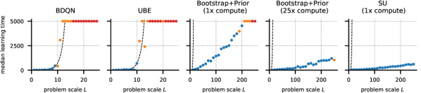
Figure 2: Median number of episodes required to learn the optimal policy on the tree MDP. Blue points indicate all 5 seeds succeeded within 5000 episodes, orange indicates only some of the runs succeeded, and red all runs failed. Dashed lines correspond to the median for a uniform exploration policy. Note the reduced size of the x-axis for BDQN and UBE.

The next proposition and its proof provide intuition for the success of SU on the tree MDP. The proof is based on a lemma stated just after the proposition (see appendix B.1 for formal treatment).

Proposition 3 (Informal statement).

Assume the SU model with: (i) fixed one-hot state-action embeddings $\phi$, (ii) uniform exploration thus far, (iii) successor representations learnt to convergence for a uniform policy. Let $s_{k}$ for $2\leq k<2L$, even, be a state visited $N$ times thus far. Then the probability of selecting up in $s_{k}$, given up was selected in $s_{0},s_{2},\ldots,s_{k-2}$, is greater than one half with probability greater than $1-\epsilon_{N}$, where $\epsilon_{N}$ decreases exponentially with $N$.

Lemma 4 (Informal statement).

Under the SU model $\smash{\hat{Q}\sim P_{\hat{Q}^{\pi}}}$ for the uniform policy $\pi$, the probability that the greedy policy $\hat{\pi}=\smash{G(\hat{Q})}$ selects up in $s_{k}$, given up was selected in $s_{0},s_{2},\ldots,s_{k-2}$, is greater than one half if there exists an even $0\leq j<k$ such that

$$\mathrm{Cov}(\hat{Q}(s_{k},\textsc{up}),\hat{Q}(s_{j},\textsc{up}))>\mathrm{Cov}(\hat{Q}(s_{k},\textsc{down}),\hat{Q}(s_{j},\textsc{up}))\,.$$

Sketch proof of proposition 3.

Under SU $\smash{\hat{Q}(s_{j},\textsc{up})}=\allowdisplaybreaks\hat{r}(s_{j},\textsc{up})+\allowdisplaybreaks\ldots+\allowdisplaybreaks\rho\hat{Q}(s_{k},\textsc{up})+\allowdisplaybreaks\smash{\rho\hat{Q}(s_{k},\textsc{down})}$ with $\smash{\rho=2^{-(\frac{k-j}{2})}}$ the probability of getting from $s_{j}$ to $s_{k}$ under the uniform policy. Note that $\smash{\hat{Q}(s_{j},\textsc{up})}$ and $\smash{\hat{Q}(s_{k},\textsc{down})}$ only share the $\smash{\hat{Q}(s_{k},\textsc{down})=\hat{r}(s_{k},\textsc{down})}$ term, whereas $\smash{\hat{Q}(s_{k},\textsc{up})}$ and $\smash{\hat{Q}(s_{j},\textsc{up})}$ share $\smash{\hat{r}(s_{j},\textsc{up}),\ldots,\hat{r}(s_{p},\textsc{down})}$, where $s_{p}$ is the state with the highest index seen so far. Thus covariance between $\smash{\hat{Q}(s_{k},\textsc{up})}$ and $\smash{\hat{Q}(s_{j},\textsc{up})}$ is higher than that between $\smash{\hat{Q}(s_{k},\textsc{down})}$ and $\smash{\hat{Q}(s_{j},\textsc{up})}$ with high probability (at least $1-\epsilon_{N}$), and the result follows from lemma 4. ∎

Proposition 3 implies that (at least under the simplifying assumption of prior exploration being uniform) SU is likely to assign higher probability to Q functions for which a greedy policy leads towards the furthest visited state (cf. the role of the state $s_{p}$ in the sketch proof). This is a strategy actively aimed for in exploration algorithms such as Go-Explore where the agent uses imitation learning to return to the furthest discovered states (Ecoffet et al., 2019).

5.2 Chain MDP from (Osband et al., 2018)

We present results on the chain environment introduced by Osband et al. (2018), described in detail in appendix C.1. Osband et al. describe their MDP as being “akin to looking for a piece of hay in a needle-stack” and state that it “may seem like an impossible task”. Figure 3 shows the scaling for Successor Uncertainties and Bootstrap+Prior for this problem. Learning time $T$ scales empirically as $\smash{\mathcal{O}(L^{2.5})}$ for SU, versus $\smash{\mathcal{O}(L^{3})}$ for Bootstrap+Prior (as reported in Osband et al., 2018).

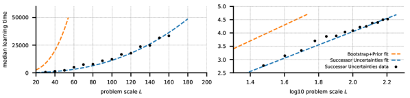
Figure 3: Learning time $T$ for SU and Bootstrap+Prior for a range of problem sizes $L$ on the chain MDP. Curve for SU is $\log_{10}T=2.5\log_{10}L-0.95$. Curve for Bootstrap+Prior is taken from figure 8 in (Osband et al., 2018).

5.3 On the success of BDQN in environments with tied actions

We briefly address prior results in the literature where BDQN is seen solving problems seemingly similar to our binary tree MDP with ease (as in, for example, figure 1 of Touati et al., 2018). The discrepancy occurs because previous work often does not randomise the effects of actions (for example Osband et al., 2016a; Plappert et al., 2018; Touati et al., 2018), i.e. if $a_{1}$ leads up in any state $s_{k}$, then $a_{1}$ leads up in all states. We refer to this as the tied actions setting. In the following proposition, we show that MDPs with tied actions are trivial for BDQN with strictly positive activations (e.g. sigmoid). We offer a similar result for ReLU in appendix B.2.

Proposition 5.

Let $\smash{\hat{Q}(s,a)=\langle\phi(s),w_{a}\rangle}$ be a Bayesian Q function model with $\phi(s)=\varphi(U1_{s})\in\mathbb{R}^{d}$, $1_{s}$ a one-hot encoding of $s$, and $\varphi$ a strictly positive activation function (e.g. sigmoid) applied elementwise. Then sampling independently from the prior $w_{a}\sim\mathcal{N}(0,\sigma_{w}^{2}I)$, $U_{hs}\sim\mathcal{N}(0,\sigma_{u}^{2})$ solves a tied action binary tree of size $L$ in $\smash{T\leq-[\log_{2}(1-2^{-d})]^{-1}}$ median number of episodes.

Proof.

Define $\Delta\coloneqq w_{\textsc{up}}-w_{\textsc{down}}$ and observe up is selected if $\smash{\hat{Q}(s,\textsc{up})-\hat{Q}(s,\textsc{down})}=\langle\phi(s),w_{\textsc{up}}-w_{\textsc{down}}\rangle>0$. By strict positivity of $\varphi$, the probability that up is always selected

$$\mathbb{P}\bigl{[}\bigcap_{j=0}^{L-1}\{\smash{\hat{Q}(s_{2j},\textsc{up})}\!>\!\smash{\hat{Q}(s_{2j},\textsc{down})}\}\bigr{]}\!\geq\!\mathbb{P}\bigl{[}\bigcap_{j=0}^{L-1}\{\langle\phi(s_{2j}),\Delta\rangle\!>\!0\}\mid\Delta\!>\!0\bigr{]}\mathbb{P}(\Delta\!>\!0)=\mathbb{P}(\Delta>0)\,,$$

where $\Delta>0$ is to be interpreted elementwise. As $\Delta\sim\mathcal{N}(0,2\sigma_{w}^{2}I)$, $\mathbb{P}(\Delta>0)=2^{-d}$ for all $L$. ∎

A single layer BDQN with one neuron can thus solve a tied action binary tree of any size $L$ in one episode (median) while completely ignoring all state information. That such an approach can be successful implies tied actions MDPs generally do not make for good exploration benchmarks.

6 Atari 2600 experiments

We have tested the SU algorithm on the standard set of 49 games from the Arcade Learning Environment, with the aim of showing that SU can be scaled to complex domains that require generalisation between states. We use a standard network architecture as in (Mnih et al., 2015; Van Hasselt et al., 2016) endowed with an extra head for prediction of $\smash{\hat{\phi}}$ and one-step value updates. More detail on our implementation, network architecture and training procedure can be found in appendix C.2.

SU obtains a median human normalised score of 2.09 (averaged over 3 seeds) after 200M training frames under the ‘no-ops start 30 minute emulator time’ test protocol described in (Hessel et al., 2018). Table 1 shows we significantly outperform competing methods. The raw scores are reported in table 2 (appendix), and the difference in human normalised score between SU and the competing algorithms for individual games is charted in figure 4. Since Azizzadenesheli et al. (2018) only report scores for a small subset of the games and use a non-standard testing procedure, we do not compare against BDQN. Osband et al. (2018), who introduce Bootstrap+Prior, do not report Atari results; we thus compare with results for the original plain Bootstrapped DQN (Osband et al., 2016a) instead.

Table 1: Human normalised Atari scores. Superhuman performance is the percentage of games on which each algorithm surpasses human performance (as reported in Mnih et al., 2015).

Algorithm	Human normalised score percentiles			Superhuman
	25%	50%	75%	performance %
Successor Uncertainties	1.06	2.09	5.95	77.55%
Bootstrapped DQN	0.76	1.60	5.16	67.35%
UBE	0.38	1.07	4.14	51.02%
DQN + $\epsilon$-greedy	0.50	1.00	3.41	48.98%

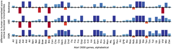
Figure 4: Bars show the difference in human normalised score between SU and Bootstrap DQN (top), UBE (middle) and DQN (bottom) for each of the 49 Atari 2600 games. Blue indicates SU performed better, red worse. SU outperforms the baselines on $36/49$, $43/49$ and $42/49$ games respectively. Y-axis values have been clipped to $[-2.5,2.5]$.

7 Conclusion

We studied the Posterior Sampling for Reinforcement Learning algorithm and its extensions within the Randomised Value Function framework, focusing on use with neural network function approximation. We have shown theoretically that exploration techniques based on the concept of propagation of uncertainty are neither sufficient nor necessary for posterior sampling exploration in sparse environments. We instead proposed posterior sampling policy matching, a property motivated by the probabilistic model over rewards and state transitions within the PSRL algorithm. Based on the theoretical insights, we developed Successor Uncertainties, a randomised value function algorithm that avoids some of the pathologies present within previous work. We showed empirically that on hard tabular examples, SU significantly outperforms competing methods, and provided theoretical analysis of its behaviour. On Atari 2600, we demonstrated Successor Uncertainties is also highly effective when combined with neural network function approximation.

Performance on the hardest exploration tasks often benefits greatly from multi-step temporal difference learning (Precup, 2000; Munos et al., 2016; O’Donoghue et al., 2018) which we believe is the most promising direction for improving Successor Uncertainties. Since modification of existing models to incorporate Successor Uncertainties is relatively simple, other standard techniques used within model-free reinforcement learning like (Schaul et al., 2015; Wang et al., 2016) can be leveraged to obtain further gains. This paper thus opens many exciting directions for future research which we hope will translate into both further performance improvements and a more thorough understanding of exploration in modern reinforcement learning.

Acknowledgements

We thank Matej Balog and the anonymous reviewers for their helpful comments and suggestions. Jiri Hron acknowledges support by a Nokia CASE Studentship.

Table 2: Raw scores for Successor Uncertainties alongside DQN, UBE and Bootstrap DQN . Test conditions: 30 minute emulator time limit and no-ops starting condition. Baselines as reported in (Hessel et al., 2018).

Game	DQN	UBE	Bootstrap DQN	SU
Alien	1,620.0	3,345.3	2,436.6	6,924.4
Amidar	978.0	1,400.1	1,272.5	1,574.4
Assault	4,280.4	11,521.5	8,047.1	3,813.8
Asterix	4,359.0	7,038.5	19,713.2	42,762.2
Asteroids	1,364.5	1,159.4	1,032.0	2,270.4
Atlantis	279,987.0	4,648,770.8	994,500.0	2,026,261.1
Bank Heist	455.0	718.0	1,208.0	1,017.4
Battle Zone	29,900.0	19,948.9	38,666.7	39,944.4
Beam Rider	8,627.5	6,142.4	23,429.8	11,652.3
Bowling	50.4	18.3	60.2	38.3
Boxing	88.0	34.2	93.2	99.7
Breakout	385.5	617.3	855.0	352.7
Centipede	4,657.7	4,324.1	4,553.5	7,049.3
Chopper Command	6,126.0	7,130.8	4,100.0	15,787.8
Crazy Climber	110,763.0	132,997.5	137,925.9	171,991.1
Demon Attack	12,149.4	25,021.1	82,610.0	183,243.2
Double Dunk	-6.6	4.7	3.0	-0.2
Enduro	729.0	30.8	1,591.0	2,216.3
Fishing Derby	-4.9	3.1	26.0	53.3
Freeway	30.8	0.0	33.9	33.8
Frostbite	797.4	546.0	2,181.4	2,733.3
Gopher	8,777.4	13,808.0	17,438.4	19,126.2
Gravitar	473.0	224.5	286.1	684.4
H.E.R.O.	20,437.8	12,808.8	21,021.3	22,050.8
Ice Hockey	-1.9	-6.6	-1.3	-2.9
James Bond	768.5	778.4	1,663.5	2,171.1
Kangaroo	7,259.0	6,101.2	14,862.5	15,751.1
Krull	8,422.3	9,835.9	8,627.9	10,103.9
Kung-Fu Master	26,059.0	29,097.1	36,733.3	50,878.9
Montezumas Revenge	0.0	499.1	100.0	0.0
Ms. Pac-Man	3,085.6	3,141.3	2,983.3	4,894.8
Name This Game	8,207.8	4,604.4	11,501.1	12,686.7
Pong	19.5	14.2	20.9	21.0
Private Eye	146.7	-281.1	1,812.5	133.3
Q*Bert	13,117.3	16,772.5	15,092.7	22,895.8
River Raid	7,377.6	8,732.3	12,845.0	17,940.6
Road Runner	39,544.0	56,581.1	51,500.0	61,594.4
Robotank	63.9	42.4	66.6	58.5
Seaquest	5,860.6	1,880.6	9,083.1	68,739.9
Space Invaders	1,692.3	2,032.4	2,893.0	13,754.3
Star Gunner	54,282.0	44,458.6	55,725.0	78,837.8
Tennis	12.2	10.2	0.0	-1.0
Time Pilot	4,870.0	5,650.6	9,079.4	9,574.4
Tutankham	68.1	218.6	214.8	247.7
Up and Down	9,989.9	12,445.9	26,231.0	29,993.4
Venture	163.0	-14.7	212.5	1,422.2
Video Pinball	196,760.4	51,178.2	811,610.0	515,601.9
Wizard Of Wor	2,704.0	8,425.5	6,804.7	15,023.3
Zaxxon	5,363.0	5,717.9	11,491.7	14,757.8

Appendix A Appendix to section 3: proofs of propositions 1 and 2

See 1

Proof.

We can w.l.o.g. assume that the distribution is symmetric around zero as centring will not affect validity of the following argument. To attain probability of taking a particular action $a$ in state $s$ greater than $\tfrac{1}{2}$, it must be that $\mathbb{P}(a=\operatorname*{argmax}_{a^{\prime}}\hat{Q}(s,a^{\prime}))>\tfrac{1}{2}$. This event can be described as

$$A\coloneqq\bigcap_{a^{\prime}\in\mathcal{A}\setminus\{a\}}\{\hat{Q}\colon\hat{Q}(s,a)>\hat{Q}(s,a^{\prime})\}\,;$$

by symmetry, the event

$$\tilde{A}\coloneqq\bigcap_{a^{\prime}\in\mathcal{A}\setminus\{a\}}\{\hat{Q}\colon\hat{Q}(s,a)<\hat{Q}(s,a^{\prime})\}\,,$$

must have the same probability as $A$. Because $\mathbb{P}(A)+\mathbb{P}(\tilde{A})\leq 1$, it must be that $\mathbb{P}(A)\leq\tfrac{1}{2}$. Since $\hat{Q}(s,a)$ is by assumption independent of any $\hat{Q}(s^{\prime},a^{\prime})$, $(s,a)\neq(s^{\prime},a^{\prime})$, the probability of executing a sequence of $L$ actions is at best (i.e. under deterministic transitions) the product of probabilities of executing a single action, which is upper bounded by $2^{-L}$. ∎

See 2

Proof.

First, let us formally define $G\colon\bar{\mathbb{R}}^{\mathcal{S}\times\mathcal{A}}\to\mathcal{A}^{\mathcal{S}}$ to be the function which maps each Q function to the corresponding greedy policy (we can w.l.o.g. assume there is some tie-breaking rule for when $\hat{Q}(s,a)=\hat{Q}(s,a^{\prime}),a\neq a^{\prime}$, e.g. taking the action with smaller index). Here, $\bar{\mathbb{R}}$ is the extended space of real numbers, and we assume the Borel $\sigma$-algebra generated by the usual interval topology; the discrete $\sigma$-algebra is assumed on $\mathcal{A}$. For product spaces, the product $\sigma$-algebra is taken. Given that the pre-image of a particular point $\hat{\pi}\in\mathcal{A}^{\mathcal{S}}$ is $\bigcap_{s\in\mathcal{S}}\{\hat{Q}\colon\hat{Q}(s,\hat{\pi}(s))\geq\hat{Q}(s,a),\forall a\}$, $G$ is measurable and thus the distribution $P_{\hat{\pi}}=G_{\#}P_{\hat{Q}}$ is well-defined for any $P_{\hat{Q}}\in\mathcal{P}(\mathbb{R}^{\mathcal{S}\times\mathcal{A}})$, and in particular for $\smash{P_{\hat{Q}}=(G\circ F^{\pi})_{\#}P_{\hat{\mathcal{T}}}}$ for any policy $\pi$.

Our proof relies on the following observation: if we sample $\hat{\pi}\sim P_{\hat{\pi}}$ and then use it to explore the environment, the distribution of actions taken in a particular state $s\in\mathcal{S}$ will be categorical with parameter $p_{s}\in\{p\in\mathbb{R}_{+}^{|\mathcal{A}|}\colon\sum_{j=1}^{|\mathcal{A}|}p_{j}=1\}$ (except for when the state $s$ is reached with probability zero under $\smash{P_{\hat{\mathcal{T}}}}$ and $\smash{P_{\hat{\pi}}}$ in which case we can set $p_{s}$, for example, to $[1/|\mathcal{A}|,\ldots,1/|\mathcal{A}|]^{\top}$ as this will not affect the following argument). Hence to achieve $G_{\#}P_{\hat{Q}^{\pi}}=P_{\hat{\pi}}$, it is sufficient to construct a model $\hat{Q}\sim P_{\hat{Q}^{\pi}}$ for which the distribution of $\operatorname*{argmax}_{a\in\mathcal{A}}\hat{Q}(s,a)$ is categorical with the parameter $p_{s}$ for all $s\in\mathcal{S}$. We achieve this using the Gumbel trick: sample $g_{sa}\sim\mathrm{Gumbel}(0,1)$ independently for each $(s,a)\in\mathcal{S}\times\mathcal{A}$, and set $\hat{Q}(s,a)=g_{sa}+\log p_{sa}$ (interpreting $\log 0=-\infty$).

To finish the proof, observe that if the inputs to the $\operatorname*{argmax}$ operator are all shifted by the same amount, or multiplied by a positive scalar, the output remains unchanged. Hence taking $\hat{Q}^{\prime}(s,a)=a+b\hat{Q}(s,a)$ for any $a\in\mathbb{R},b>0$ will also result in the desired distribution over exploration policies. We can thus take the $(s,a)$ for which $\mathbb{V}_{F_{\#}^{\pi}P_{\hat{\mathcal{T}}}}[\hat{Q}(s,a)]>0$ and pick $b>0$ so that $\mathbb{V}_{P_{\hat{Q}^{\pi}}}[\hat{Q}(s,a)]\neq\mathbb{V}_{F_{\#}^{\pi}P_{\hat{\mathcal{T}}}}[\hat{Q}(s,a)]$ which will be always possible as $\mathbb{V}(b\hat{Q}(s,a))$ is $b^{2}\mathbb{V}(g_{sa})=b^{2}\frac{\pi^{2}}{6}$ if $p_{sa}>0$ and is undefined otherwise. ∎

Appendix B Appendix to section 5

B.1 Proofs for section 5.1

In what follows, the binary tree MDP of size $L$ introduced in figure 1 is assumed. We further assume $\smash{\phi}$ is given and maps each state-action to its one-hot embedding. As all of the following arguments are independent of the mapping from the actions $\{a_{1},a_{2}\}$ to the movements $\{\textsc{up},\textsc{down}\}$, we use $\mathcal{A}=\{\textsc{up},\textsc{down}\}$ directly for improved clarity.

To prove lemma 4, we will need lemmas 6 to 9 which we state and prove now.

Lemma 6.

After any number of posterior updates, the SU reward distribution is multivariate normal with all rewards mutually independent. Furthemore, under the SU Q function model $\smash{\hat{Q}\sim P_{\hat{Q}^{\pi}}}$ for any policy $\pi$, and even state indices $0\leq j<k$

$$\mathrm{Cov}(\hat{Q}(s_{k},\textsc{up}),\hat{Q}(s_{j},\textsc{down}))=\mathrm{Cov}(\hat{Q}(s_{k},\textsc{down}),\hat{Q}(s_{j},\textsc{down}))=0\,.$$

Proof.

Inspecting equations (2) and (3), it is easy to see that neither $\hat{Q}(s_{k},\textsc{up})$ and $\hat{Q}(s_{j},\textsc{down})$ nor $\hat{Q}(s_{k},\textsc{down})$ and $\hat{Q}(s_{j},\textsc{down})$ share any reward terms, since $j<k$ by assumption and the empirical transition frequencies used to construct $\smash{P_{\hat{Q}^{\pi}}}$ will always be zero if the true transition probability is zero (recall that down always terminates the episode). Hence assuming that the successor features were successfully learnt, i.e. $\hat{\psi}^{\pi}=\psi^{\pi}$, it is sufficient to show that the individual rewards are independent for SU. To see that this is the case, observe that the assumed one-hot encoding of state-actions implies that SU reward distribution will be a multivariate Gaussian with diagonal covariance after any number of updates which implies the desired independence. ∎

Lemma 7.

Under the SU model $\smash{\hat{Q}\sim P_{\hat{Q}^{\pi}}}$ for any policy $\pi$, the random vector $\Delta$, $\Delta_{k/2}\coloneqq\hat{Q}(s_{k},\textsc{up})-\hat{Q}(s_{k},\textsc{down})$, follows a zero mean Gaussian distribution with $\mathrm{Cov}(\Delta_{k/2},\Delta_{j/2})=\mathrm{Cov}(\hat{Q}(s_{k},\textsc{up}),\hat{Q}(s_{j},\textsc{up}))-\mathrm{Cov}(\hat{Q}(s_{k},\textsc{down}),\hat{Q}(s_{j},\textsc{up})))$ for any even indices $0\leq j<k$.

Proof.

The Gaussianity of the joint distribution of $\Delta_{j/2}$ and $\Delta_{k/2}$ follows from the linearity property of multivariate normal distributions. For the covariance, observe

$$\mathrm{Cov}(\Delta_{k/2},\Delta_{j/2}) =\mathrm{Cov}(\hat{Q}(s_{k},\textsc{up})-\hat{Q}(s_{k},\textsc{down}),\hat{Q}(s_{j},\textsc{up})-\hat{Q}(s_{j},\textsc{down}))$$

$$=\begin{aligned} &\mathrm{Cov}(\hat{Q}(s_{k},\textsc{up}),\hat{Q}(s_{j},\textsc{up}))-\mathrm{Cov}(\hat{Q}(s_{k},\textsc{down}),\hat{Q}(s_{j},\textsc{up}))-\\ &\mathrm{Cov}(\hat{Q}(s_{k},\textsc{up}),\hat{Q}(s_{j},\textsc{down}))+\mathrm{Cov}(\hat{Q}(s_{k},\textsc{down}),\hat{Q}(s_{j},\textsc{down}))\end{aligned}$$

$$=\mathrm{Cov}(\hat{Q}(s_{k},\textsc{up}),\hat{Q}(s_{j},\textsc{up}))-\mathrm{Cov}(\hat{Q}(s_{k},\textsc{down}),\hat{Q}(s_{j},\textsc{up})))\,,$$

where we used bilinearity of the covariance operator and then applied lemma 6. ∎

Lemma 8.

Under the SU model $\smash{\hat{Q}\sim P_{\hat{Q}^{\pi}}}$ for the uniform policy $\pi$, and even indices $0\leq j<k$

$$\mathrm{Cov}(\hat{Q}(s_{k},\textsc{up}),\hat{Q}(s_{j},\textsc{up})) >\mathrm{Cov}(\hat{Q}(s_{k},\textsc{down}),\hat{Q}(s_{j},\textsc{up})))$$

$$\iff \mathbb{V}(\hat{Q}(s_{k},\textsc{up})) >\mathbb{V}(\hat{Q}(s_{k},\textsc{down}))\,.$$

Proof.

Analogously to the proof of lemma 7, we see that under the uniform policy

$$\mathrm{Cov}(\hat{Q}(s_{k},\textsc{up}),\hat{Q}(s_{j},\textsc{up}))$$

$$=\, \mathrm{Cov}(\hat{Q}(s_{k},\textsc{up}),\,\hat{r}(s_{j},\textsc{up})+2^{-1}\hat{r}(s_{j+2},\textsc{up})+\ldots+2^{-(\frac{k-j}{2})}\hat{Q}(s_{k},\textsc{up}))$$

$$= 2^{-(\frac{k-j}{2})}\, \mathrm{Cov}(\hat{Q}(s_{k},\textsc{up}),\hat{Q}(s_{k},\textsc{up}))=2^{-(\frac{k-j}{2})}\,\mathbb{V}(\hat{Q}(s_{k},\textsc{up}))\,,$$

where the $2^{-l}$ terms correspond to the probability of getting to $s_{l}$ from $(s_{j},\textsc{up})$, $l=1,2,\ldots,\frac{k-j}{2}$, and we used bilinearity of the covariance operator and then applied lemma 6. An analogous argument yields $\mathrm{Cov}(\hat{Q}(s_{k},\textsc{down}),\hat{Q}(s_{j},\textsc{up}))=2^{-(\frac{k-j}{2})}\mathbb{V}(\hat{Q}(s_{k},\textsc{down}))$, concluding the proof. ∎

Lemma 9.

For a $d$-dimensional centred Gaussian random vector $\Delta\sim\mathcal{N}(0,\Sigma)$ with $\mathrm{Cov}(\Delta_{d},\Delta_{i})>0$ for all $i=1,\ldots,d-1$, the following bound holds: $\mathbb{P}(\Delta_{d}>0\mid\Delta_{1}>0,\ldots,\Delta_{d-1}>0)>1/2$.

Proof.

Notice that $\Delta$ and $\Sigma^{1/2}X$, $X\sim\mathcal{N}(0,1)$, are equal in distribution which allows us to set $\Delta_{i}=\langle v_{i},X\rangle$, with $v_{i}\in\mathbb{R}^{d}$ the $i$^th row of $\Sigma^{1/2}$. Let $R_{v}\colon\mathbb{R}^{d}\to\mathbb{R}^{d}$ be the reflection against the orthogonal complement of $v$, i.e.

$$R_{v}(x)=x-2\frac{\langle x,v\rangle}{\langle v,v\rangle}v\,.$$

It is easy to see that $\langle v,R_{v}(x)\rangle=-\langle v,x\rangle$ and consequently $R_{v}(R_{v}(x))=x$. The main idea of this proof is to partition $\mathbb{R}^{d}$ into the half-spaces $\{x\colon\langle v_{i},x\rangle>0\}$ and $\{x\colon\langle v_{i},R_{v_{d}}(x)\rangle>0\}$, $i=1,\ldots,d-1$, and reason about the value $\langle v_{d},x\rangle$ takes in each.

First, we define the conditioning set $E\coloneqq\{x\colon\langle v_{i},x\rangle>0\,,\forall i=1,\ldots,d-1\}$ and observe that $\mathbb{P}(X\in E)>0$ so all we need to prove is $\mathbb{E}[\mathbbm{1}_{\langle v_{d},X\rangle>0}\mathbbm{1}_{E}]>\mathbb{E}[\mathbbm{1}_{\langle v_{d},X\rangle\leq 0}\mathbbm{1}_{E}]$, where $\mathbbm{1}_{E}$ is the indicator function of the set $E$. To do so, we define $U\coloneqq\{x\colon\langle v_{i},R_{v_{d}}(x)\rangle>0\,,\forall i=1,\ldots,d-1\}$, $A_{+}\coloneqq E\,\cap\,U$, $A_{-}\coloneqq E\,\cap\,U^{\mathsf{c}}$, split the integral $\int_{E}\mathbbm{1}_{\{\langle v_{d},X\rangle>0\}}(x)\phi(x)\,\mathrm{d}x$ into $\int_{A_{+}}\mathbbm{1}_{\{\langle v_{d},X\rangle>0\}}(x)\phi(x)\,\mathrm{d}x+\int_{A_{-}}\mathbbm{1}_{\{\langle v_{d},X\rangle>0\}}(x)\phi(x)\,\mathrm{d}x$ ($\phi$ is the standard normal density function; analogously for $\mathbbm{1}_{\{\langle v_{d},X\rangle\leq 0\}}$), and consider $X\in A_{+}$ and $X\in A_{-}$ separately:

(I) $X\in A_{+}$: Take any $x,v\in\mathbb{R}^{d}$ and define the orthogonal projection map on $v$, $B_{v}\coloneqq vv^{\top}/\|v\|_{2}^{2}$, and the corresponding projections of $x$, $x_{v}\coloneqq B_{v}x\,,x_{v}^{\bot}=(I-B_{v})x$, so that $x=x_{v}+x_{v}^{\bot}$. Since

$$\|x\|_{2}^{2}=\|x_{v}+x_{v}^{\bot}\|_{2}^{2}=\|x_{v}\|_{2}^{2}+\|x_{v}^{\bot}\|_{2}^{2}=\|-x_{v}+x_{v}^{\bot}\|_{2}^{2}=\|R_{v}(x)\|_{2}^{2}\,,$$

it follows that $\phi(x)=\phi(R_{v_{d}}(x))$. Noticing further that $R_{v_{d}}(x)=(I-2B_{v_{d}})x$ and recalling $R_{v_{d}}(R_{v_{d}}(x))=x$, we have $|\det\nabla_{x}R_{v_{d}}(x)|=|-1|=1$. The crucial observation here is $\langle x,v_{d}\rangle>0\iff\langle x_{v_{d}},v_{d}\rangle>0$, $\langle x,v_{d}\rangle\leq 0\iff\langle R_{v_{d}}(x),v_{d}\rangle>0$ (up to null sets), and that $A_{+}=R_{v_{d}}[A_{+}]=\{R_{v_{d}}(x)\colon x\in A_{+}\}$ which follows from the definition of the set $A_{+}$. In particular this means that whenever $x\in A_{+}$ then also $-x\in A_{+}$, and thus by the above established symmetry and the change of variable formula, $\int_{A_{+}}\mathbbm{1}_{\{\langle v_{d},X\rangle>0\}}(x)\phi(x)\,\mathrm{d}x=\int_{A_{+}}\mathbbm{1}_{\{\langle v_{d},X\rangle\leq 0\}}(x)\phi(x)\,\mathrm{d}x$, i.e. the conditional probabilities of both $A_{+}\,\cap\,\{\langle v_{d},X\rangle>0\}$ and $A_{+}\,\cap\,\{\langle v_{d},X\rangle\leq 0\}$ are equal.

(II) $X\in A_{-}$: Notice that for any $i=1,\ldots,d-1$

$$\langle v_{i},R_{v_{d}}(x)\rangle=\langle v_{i},x\rangle-2\frac{\langle v_{d},x\rangle}{\|v_{d}\|_{2}^{2}}\langle v_{d},v_{i}\rangle\,.$$

Hence if $\langle v_{d},x\rangle\leq 0$ then $\langle v_{i},R_{v_{d}}(x)\rangle\geq\langle v_{i},x\rangle>0$ from the definition $\langle v_{d},v_{i}\rangle=\mathrm{Cov}(\Delta_{d},\Delta_{i})$ and the assumption $\mathrm{Cov}(\Delta_{d},\Delta_{i})>0$. Now by the definition of $U$ in $A_{-}=E\,\cap\,U^{\mathsf{c}}$, for any $x\in A_{-}$, there must exist $i\in\{1,\ldots,d-1\}$ such that $\langle v_{i},R_{v_{d}}(x)\rangle\leq 0$ which implies $\langle v_{d},x\rangle>0$ by the above argument. It is thus sufficient to establish $\mathbb{P}(X\in A_{-})>0$ to complete the proof as the intersection $A_{-}\,\cap\,\{\langle v_{d},X\rangle\leq 0\}$ is empty.

Since $\langle v_{d},v_{i}\rangle=\mathrm{Cov}(\Delta_{d},\Delta_{i})>0$, $v_{d}\in E$ and $\langle v_{i},R_{v_{d}}(v_{d})\rangle=-\langle v_{i},v_{d}\rangle<0\,,\forall i=1,\ldots,d-1$, we have $v_{d}\in A_{-}$. We can thus construct a convex polytope $V\subseteq A_{-}$ such that $\mathbb{P}(X\in V)>0$. Specifically, pick some $i\in\{1,\ldots,d-1\}$, for example $i=\operatorname*{argmax}_{i\in\{1,\ldots,d-1\}}\langle v_{d},v_{i}\rangle$, and set $\kappa\coloneqq\max_{k,l\in\{1,\ldots,d\}}|\langle v_{k},v_{l}\rangle|=\max_{k\in\{1,\ldots,d\}}\|v_{k}\|_{2}^{2}>0$. Now define

$$V\coloneqq\{x\colon x=u+v_{d}+\sum_{j=1}^{d-1}\alpha_{j}v_{j}\,,\alpha_{j}\in[0,\tfrac{\langle v_{d},v_{i}\rangle}{\kappa(d-1)})\,,u\in\mathrm{span}(v_{1},\ldots,v_{d})^{\bot}\}\,,$$

where $\mathrm{span}(v_{1},\ldots,v_{d})^{\bot}$ is the orthogonal complement of the linear span of the vectors $(v_{1},\ldots,v_{d})$. Clearly $V\subseteq E$ as for any $x\in V$, $\langle v_{i},x\rangle>0$ from the bound on the coefficients $\alpha$. To see that $x\in V\implies x\in U^{\mathsf{c}}$, note

$$\langle v_{i},R_{v_{d}}(x)\rangle=-\langle v_{i},v_{d}\rangle+\sum_{j=1}^{d-1}\underbrace{\alpha_{j}}_{\geq 0}\biggl{[}\langle v_{i},v_{j}\rangle-2\underbrace{\frac{\langle v_{d},v_{i}\rangle}{\|v_{d}\|_{2}^{2}}\langle v_{j},v_{d}\rangle}_{>0}\biggr{]}\,.$$

Since the first and last terms are strictly negative, we just need to control the second term. We again apply the definition of $V$ to bound $\sum_{j}\alpha_{j}\langle v_{i},v_{j}\rangle<\langle v_{i},v_{d}\rangle$ which implies $\langle v_{i},R_{v_{d}}(x)\rangle<0$ for every $x\in V$. Thus $V\subseteq A_{-}$ and because $V$ has non-zero volume, its probability under $\mathcal{N}(0,I)$ will be positive. Hence $\int_{A_{-}}\mathbbm{1}_{\{\langle v_{d},X\rangle>0\}}(x)\phi(x)\,\mathrm{d}x>\int_{A_{-}}\mathbbm{1}_{\{\langle v_{d},X\rangle\leq 0\}}\phi(x)\,\mathrm{d}x=0$. ∎

We are now ready to prove lemma 4.

Lemma 10 (Formal statement).

Let $\smash{\hat{\pi}\sim P_{\hat{\pi}}=G_{\#}P_{\hat{Q}^{\pi}}}$ where $\smash{\hat{Q}\sim P_{\hat{Q}^{\pi}}}$ is the SU model for the uniform policy $\pi$. For $2\leq k<2L$ even, define $\smash{U_{k}=\{\hat{\pi}\colon\hat{\pi}(s_{0})=\ldots=\hat{\pi}(s_{k-2})=\delta_{\textsc{up}}\}}$ where $\smash{\delta_{\textsc{up}}}$ is the policy of selecting up with probability one. Then $\smash{P_{\hat{\pi}}(\hat{\pi}(s_{k})=\delta_{\textsc{up}}\mid\hat{\pi}\in U_{k})>1/2}$ if there exists an even $0\leq j<k$ such that $\mathrm{Cov}(\hat{Q}(s_{k},\textsc{up}),\hat{Q}(s_{j},\textsc{up}))>\mathrm{Cov}(\hat{Q}(s_{k},\textsc{down}),\hat{Q}(s_{j},\textsc{up}))\,.$

Proof.

Under $P_{\hat{\pi}}$, $G(\hat{Q})=\delta_{\textsc{up}}$ iff $\Delta_{k/2}=\hat{Q}(s_{k},\textsc{up})-\hat{Q}(s_{k},\textsc{down})>0$. By lemma 7, the distribution of the random vector $\Delta=[\Delta_{0},\Delta_{1},\ldots,\Delta_{k/2}]^{\top}$ is a zero mean Gaussian, and in particular

$$P_{\hat{\pi}}(\hat{\pi}=\delta_{\textsc{up}}\mid\hat{\pi}\in U_{k})=\mathbb{P}(\Delta_{k/2}>0\mid\Delta_{0}>0,\ldots,\Delta_{k/2-1}>0)\,.$$

To prove the desired claim, we therefore need to show that existence of even $0\leq j<k$ such that $\smash{\mathrm{Cov}(\hat{Q}(s_{k},\textsc{up}),\hat{Q}(s_{j},\textsc{up}))>\mathrm{Cov}(\hat{Q}(s_{k},\textsc{down}),\hat{Q}(s_{j},\textsc{up}))\,,}$ implies $\mathbb{P}(\Delta_{k/2}>0\mid\Delta_{0}>0,\ldots,\Delta_{k/2-1}>0)>1/2$. The statement follows from:

$$\mathrm{Cov}(\hat{Q}(s_{k},\textsc{up}),\hat{Q}(s_{j},\textsc{up}))>\mathrm{Cov}(\hat{Q}(s_{k},\textsc{down}),\hat{Q}(s_{j},\textsc{up}))\,\text{, for some even }0\leq j<k$$

$$\overset{\text{lemma\leavevmode\nobreak\ \ref{lem:var-condition}}}{\iff}\mathrm{Cov}(\hat{Q}(s_{k},\textsc{up}),\hat{Q}(s_{j},\textsc{up}))>\mathrm{Cov}(\hat{Q}(s_{k},\textsc{down}),\hat{Q}(s_{j},\textsc{up}))\,\text{, for all even }0\leq j<k$$

$$\overset{\text{lemma\leavevmode\nobreak\ \ref{lem:delta-covariance}}}{\iff}\mathrm{Cov}(\Delta_{k/2},\Delta_{j/2})>0\,\text{, for all even }0\leq j<k$$

$$\overset{\text{lemma\leavevmode\nobreak\ \ref{lem:corr_implies_positivity}}}{\iff}\mathbb{P}(\Delta_{k/2}>0\mid\Delta_{0}>0,\ldots,\Delta_{k/2-1}>0)>1/2\,.$$

∎

Proposition 3 (Formal statement).

Assume the SU model with: (i) one-hot state-action embeddings $\phi$, (ii) uniform exploration thus far, (iii) successor representations learnt to convergence for a uniform policy. For $2\leq k<2L$ even, let $s_{k}$ be a state visited $N$ times thus far, and $\pi$, $\smash{\hat{Q}\sim P_{\hat{Q}^{\pi}}}$, $\smash{\hat{\pi}\sim P_{\hat{\pi}}}$, and $U_{k}$ be defined as in lemma 4. Then

$$\smash{P_{\hat{\pi}}(\hat{\pi}(s_{k})=\delta_{\textsc{up}}\mid\hat{\pi}\in U_{k})>P_{\hat{\pi}}(\hat{\pi}(s_{k})=\delta_{\textsc{down}}\mid\hat{\pi}\in U_{k})}\,,$$

with probability greater than $1-\epsilon_{N}$, where $\epsilon_{N}<0.75^{N}e^{-\frac{N}{50}}+(1-0.75^{N})e^{-0.175N}$.

Proof.

By lemma 4, we know that $\smash{P_{\hat{\pi}}(\hat{\pi}(s_{k})=\delta_{\textsc{up}}\mid\hat{\pi}\in U_{k})>P_{\hat{\pi}}(\hat{\pi}(s_{k})=\delta_{\textsc{down}}\mid\hat{\pi}\in U_{k})}$ holds if $\mathrm{Cov}(\hat{Q}(s_{k},\textsc{up}),\hat{Q}(s_{j},\textsc{up}))>\allowdisplaybreaks\mathrm{Cov}(\hat{Q}(s_{k},\textsc{down}),\hat{Q}(s_{j},\textsc{up}))$ for some $j=0,2,\ldots,k-2$. By lemma 8, this condition is equivalent to requiring $\mathbb{V}(\hat{Q}(s_{k},\textsc{up}))>\mathbb{V}(\hat{Q}(s_{k},\textsc{down}))$. Our approach is thus based on lower bounding the probability of the event

$$\{\hat{Q}\colon\mathbb{V}(\hat{Q}(s_{k},\textsc{up}))>\mathbb{V}(\hat{Q}(s_{k},\textsc{down}))\}\,.$$ (5)

The rest of the proof is divided into two stages:

1. We derive a crude bound $\smash{\Upsilon}_{1}(\hat{Q}(s_{k},\textsc{up}))\leq\mathbb{V}(\hat{Q}(s_{k},\textsc{up}))$ and compute a lower bound on the probability of the event $\smash{\Upsilon}_{1}(\hat{Q}(s_{k},\textsc{up}))>\mathbb{V}(\hat{Q}(s_{k},\textsc{down}))$.

2. We then derive a tighter lower bound $\smash{\Upsilon}_{2}(\hat{Q}(s_{k},\textsc{up}))$, and again compute a lower bound on the probability of the event $\smash{\Upsilon}_{2}(\hat{Q}(s_{k},\textsc{down}))>\mathbb{V}(\hat{Q}(s_{k},\textsc{down}))$.

(I) The bound $\smash{\Upsilon_{1}(\hat{Q}(s_{k},\textsc{up}))\leq\mathbb{V}(\hat{Q}(s_{k},\textsc{up}))}$ will correspond to a worst case assumption about the distribution of data available from exploration, and $\smash{\Upsilon_{2}(\hat{Q}(s_{k},\textsc{up}))}$ to a less pessimistic scenario. The change of setup involved in moving from the first bound to the second will be illustrative of the manner in which, under the SU model, the more states the agent has previously observed beyond $s_{k}$, the more likely it is to satisfy the condition from equation (5) and consequently $\mathrm{Cov}(\hat{Q}(s_{k},\textsc{up}),\hat{Q}(s_{j},\textsc{up}))>\allowdisplaybreaks\mathrm{Cov}(\hat{Q}(s_{k},\textsc{down}),\hat{Q}(s_{j},\textsc{up}))$ for all $j=0,2,\ldots,k-2$.

From lemma 6, we know that the SU model of rewards will be a zero mean Gaussian with a diagonal covariance. In particular, the covariance takes the form $(\theta^{-1}I+\beta^{-1}\sum_{t}\phi_{t}\phi_{t}^{\top})^{-1}$, where recall $\theta$ is the prior and $\beta$ is the likelihood variance, implying that the diagonal entries will be $\nu(n)\coloneqq(\theta^{-1}+\beta^{-1}n)^{-1}$ where $n$ is the number of times the corresponding state-action was observed.

Recall that the agent has previously visited the state $s_{k}$ $N$ times. We will write $\smash{N_{1}}$ for the number of times we have observed $(s_{k},\textsc{up})$ so far, $\smash{N_{2}}$ for the number of times $(s_{k},\textsc{up})$ and $(s_{k+2},\textsc{up})$ have both been observed within a single episode, and so forth. Observe

$$\mathbb{V}(\hat{Q}(s_{k},\textsc{up})) =\begin{aligned} &\nu(N_{1})+2^{-1}(\nu(N_{2})+\nu(N_{1}-N_{2}))+\\ &\mathbbm{1}_{N_{3}>0}2^{-2}(\nu(N_{3})+\nu(N_{2}-N_{3})+\mathbbm{1}_{N_{4}>0}\ldots)\end{aligned}$$

$$\geq\nu(N_{1})+2^{-1}(\nu(N_{2})+\nu(N_{1}-N_{2}))$$

We now minimise $\nu(N_{2})+\nu(N_{1}-N_{2})$ with respect to $N_{2}$, finding the minima to occur at $N_{2}=N_{1}$ and $N_{2}=0$, in both cases giving the bound

$$\Upsilon_{1}(\hat{Q}(s_{k},\textsc{up}))\coloneqq\frac{3}{2}\nu(N_{1})+\frac{1}{2}\nu(0)\leq\mathbb{V}(\hat{Q}(s_{k},\textsc{up}))$$

This bound can be interpreted as assuming that after taking action up, the agent has always proceeded to move down, thus terminating the episode. We now compute a lower bound on the probability that $\Upsilon_{1}(\hat{Q}(s_{k},\textsc{up}))>\mathbb{V}(\hat{Q}(s_{k},\textsc{down}))$, in terms of $N_{1}$. We have

$$\Upsilon_{1}(\hat{Q}(s_{k},\textsc{up}))-\mathbb{V}(\hat{Q}(s_{k},\textsc{down}))=\frac{3}{2}\nu(N_{1})-\nu(N-N_{1})+\frac{1}{2}\nu(0)>\frac{3}{2}\nu(N_{1})-\nu(N-N_{1})$$

which is greater than zero when $\theta^{-1}+\beta^{-1}(3N-5N_{1})>\beta^{-1}(3N-5N_{1})>0$, i.e. whenever $\smash{N_{1}<\frac{3N}{5}}$. By Hoeffding’s inequality, $\mathbb{P}(N_{1}\geq\frac{(1+\delta)N}{2})\leq e^{-\frac{\delta^{2}N}{2}}$. Thus, letting $\delta=5^{-1}$, $\smash{\mathbb{V}(\hat{Q}(s_{k},\textsc{up}))>\mathbb{V}(\hat{Q}(s_{k},\textsc{down}))}$ holds with probability greater than $1-e^{-\frac{N}{50}}$.

(II) Notice that we have obtained the $\Upsilon_{1}$ bound by considering the worst case scenario for $N_{2}$, namely $N_{2}=0$. Here we derive a tighter bound by treating the two cases, $N_{2}=0$ and $N_{2}>0$, separately. For $N_{2}>0$, we follow an approach analogous to (I): we assume the “next” worst-case scenario, which is easily seen to be $N_{3}=0$, and compute a lower bound on $\smash{\mathbb{V}(\hat{Q}(s_{k},\textsc{up}))}$

$$\Upsilon_{2}(\hat{Q}(s_{k},\textsc{up}))\coloneqq\nu(N_{1})+\nu(N_{2})+\frac{1}{2}\nu(N_{1}-N_{2})\,.$$

After some algebra, we obtain $\smash{\Upsilon_{2}(\hat{Q}(s_{k},\textsc{up}))>\mathbb{V}(\hat{Q}(s_{k},\textsc{down}))}$ for all $N_{2}>0$ and $N_{1}\leq\frac{1}{41}(27+4\sqrt{2})N\eqqcolon c\,.$ We thus only need to bound the probability of $N_{1}>c$. Using Hoeffding’s inequality as in (I) for a suitably chosen $\delta$, we see $\mathbb{P}(N_{1}>c)\leq\exp\{-\frac{(13+8\sqrt{2})^{2}}{3362}N\}<e^{-0.175N}$. For $N_{2}=0$, we use the bound from part (I), and thus the only thing remaining is to compute the probability of $N_{2}=0$:

$$\mathbb{P}(N_{2}=0) =\textstyle{\sum}_{K=0}^{N}\mathbb{P}(N_{2}=0\mid N_{1}=K)\mathbb{P}(N_{1}=K)=\textstyle{\sum}_{K=0}^{N}\,2^{-K}2^{-N}\binom{N}{K}$$

$$=\textstyle{\sum}_{K=0}^{N}\binom{N}{K}\,4^{-K}2^{K-N}=(4^{-1}+2^{-1})^{N}=0.75^{N}\,.$$

Combining the above results, we see that $\smash{\mathbb{V}(\hat{Q}(s_{k},\textsc{up}))>\mathbb{V}(\hat{Q}(s_{k},\textsc{down}))}$ will hold with probability greater than $1-\epsilon_{N}$ where $\epsilon_{N}<0.75^{N}e^{-\frac{N}{50}}+(1-0.75^{N})e^{-0.175N}$. ∎

B.2 Proofs for section 5.3

The following is an extension of proposition 5 to activations such as ReLU, Leaky ReLU, or Tanh.

Proposition 11.

Consider the same setting as in proposition 5 with the exception that $\varphi$ for which $\varphi[(0,\infty)]=\{\varphi(x):x>0\}\subseteq(0,\infty)$. Then sampling independently form the prior $w_{a}\sim\mathcal{N}(0,\sigma_{w}^{2}I)$, $U_{hs}\sim\mathcal{N}(0,\sigma_{u}^{2})$ solves a tied action binary tree of size $L$ in $T\leq-[\log_{2}(1-2^{-d}(1-2^{-d})^{L})]^{-1}$ median number of episodes, or approximately ${-[\log_{2}(1-2^{-d})]^{-1}}$ for $d\geq 10$.

Proof.

As in the proof of proposition 5, let us define $\Delta\coloneqq w_{\textsc{up}}-w_{\textsc{down}}$ and observe up is selected if $\smash{\hat{Q}(s,\textsc{up})-\hat{Q}(s,\textsc{down})}=\langle\phi(s),w_{\textsc{up}}-w_{\textsc{down}}\rangle>0$. We can thus lower bound

$$\mathbb{P}\bigl{[}\bigcap_{j=0}^{L-1}\{\smash{\hat{Q}(s_{2j},\textsc{up})}\!>\!\smash{\hat{Q}(s_{2j},\textsc{down})}\}\bigr{]}\!\geq\!\mathbb{P}\bigl{[}\bigcap_{j=0}^{L-1}\{\langle\phi(s_{2j}),\Delta\rangle\!>\!0\}\mid\Delta\!>\!0\bigr{]}\mathbb{P}(\Delta\!>\!0)\,,$$

where $\Delta>0$ is meant elementwise. As $\Delta\sim\mathcal{N}(0,2\sigma_{w}^{2}I)$, $\mathbb{P}(\Delta>0)=2^{-d}$ for all $L$. By independence $\mathbb{P}\bigl{[}\bigcap_{j=0}^{L-1}\{\langle\phi(s_{2j}),\Delta\rangle\!>\!0\}\mid\Delta\!>\!0\bigr{]}=\prod_{j=0}^{L-1}\mathbb{P}(\{\phi(s_{2j})>0\})$ where $>$ is to be interpreted elementwise. From the assumption $\varphi[(0,\infty)]\subseteq(0,\infty)$ and the assumed $\phi(s)=\varphi(U1_{s})$, $U_{hs}\sim\mathcal{N}(0,\sigma_{u}^{2})$, we have $\mathbb{P}(\{\phi(s)>0\})\geq 1-2^{-d}$, which implies that probability of success within a single episode is lower bounded by $2^{-d}(1-2^{-d})^{L}$. The result follows by substituting this probability into the formula for the median of a geometric distribution. ∎

Appendix C Appendix to section 5: implementation & experimental details

Pseudocode for SU. Quantities superscripted with $\smash{\dagger}$ are treated as fixed during optimisation.

Algorithm 1 Successor Uncertainties with posterior sampling

Neural networks $\hat{\psi}$ and $\hat{\phi}$; weight vector $\hat{w}$; prior variance $\theta>0$; likelihood variance $\beta>0$; covariance decay factor $\zeta\in[0,1]$; $\textsc{batch\_size}\in\mathbb{N}$; $\textsc{learning\_rate}>0$; environment Env; action set $\mathcal{A}$; discount factor $\gamma\in[0,1)$.

initialise $\Lambda\leftarrow\theta^{-1}I$, $\hat{\Sigma}_{w}\leftarrow\Lambda^{-1}$

for each episode do

     sample $w\sim N(\hat{w},\hat{\Sigma}_{w})$

     $s\leftarrow\textsc{env.reset}()$

     repeat

         $a\leftarrow\operatorname*{argmax}_{z\in\mathcal{A}}\langle\hat{\psi}(s,z),w\rangle$

         $s^{\prime},r,done\leftarrow\textsc{env.interact}(s)$

         $\mathcal{D}\leftarrow\mathcal{D}\cup\{(s,a,r,s^{\prime},done)\}$

         $\mathcal{B}\sim\textsc{Uniform}(\mathcal{D},\textsc{batch\_size})$

         $\ell\leftarrow\sum_{b\in\mathcal{B}}\textsc{SU\_Loss}(b,\hat{\Sigma}_{w})$

         $\hat{\phi},\hat{\psi},\hat{w}\leftarrow\textsc{SGD.step}(\ell,\textsc{learning\_rate})$

         $\Lambda\leftarrow\zeta\Lambda+\beta^{-1}\hat{\phi}(s,a)\hat{\phi}(s,a)^{\top}$

         $s\leftarrow s^{\prime}$

     until $done$

     $\hat{\Sigma}_{w}\leftarrow\Lambda^{-1}$

end for

function SU_Loss(experience_tuple, $\hat{\Sigma}_{w}$)

     $s,a,r,s,done\leftarrow\textsc{experience\_tuple}$

     sample $w\sim N(\hat{w},\hat{\Sigma}_{w})$

     $a^{\prime}\leftarrow\operatorname*{argmax}_{z\in\mathcal{A}}\langle\hat{\psi}(s,z),w\rangle$

     $y_{Q}\leftarrow\begin{cases}0&\mathrm{if}\ done\\ \gamma\langle\hat{w},\hat{\psi}(s^{\prime},a^{\prime})\rangle&\mathrm{otherwise}\end{cases}$

     $y_{SF}\leftarrow\begin{cases}0&\mathrm{if}\ done\\ \gamma\hat{\psi}(s^{\prime},a^{\prime})&\mathrm{otherwise}\end{cases}$

     return $|\langle\hat{w},\hat{\phi}(s,a)\rangle-r|^{2}+\|\hat{\psi}(s,a)-\hat{\phi}(s,a)-y_{SF}^{\dagger}\|_{2}^{2}+|\langle\hat{w},\hat{\psi}(s,a)\rangle-r-y_{Q}^{\dagger}|^{2}$

end function

C.1 Appendix to sections 5.1 and 5.2: tabular experiments

Neural network architecture

The architecture used for tabular experiments consists of:

1. A neural network mapping one-hot encoded state vectors and one-hot encoded action vectors to a hidden layer $\hat{\phi}(s,a)$, and then to reward prediction $\hat{r}(s,a)$ via weights $\hat{w}$. Weights mapping state vectors to hidden layer are initialised using a folded Xavier normal initialisation and followed by ReLU activation. Weights $\hat{w}$ are initialised to zero, consistent with a Bayesian linear regression model with a zero mean prior.

2. A set of weights that linearly maps state-action vectors to $\hat{\psi}(s,a)$.

Binary tree MDP

Table 3 contains the hyperparameters considered during gridsearch and the final values used to produce figure 2. Hyperparameter values are not included for UBE and BDQN, as they do not affect performance (that is, BDQN and UBE perform uniformly random exploration for all hyperparameter settings). All methods used one layer fully connected ReLU networks, Xavier initialisation, and a replay buffer of size 10,000. Hyperparameters for all methods were selected by gridsearch on a $L=100$ sized binary tree. Hyperparameters were then kept fixed as binary tree size $L$ was varied.

Table 3: Binary tree experiment algorithm hyperparameters gridsearch sets and values used for Successor Uncertainties, Bootstrap+Prior (1x compute) and Bootstrap+Prior (25x compute).

		Algorithm
Hyperparameter	Gridsearch set	SU	B+P 1x	B+P 25x
Gradient steps per episode	—	10	10	250
Hidden size	$\{20,40\}$	20	20	20
Prior variance $\theta$	$\{1,10^{2},10^{4}\}$	$10^{4}$	—	—
Likelihood variance $\beta$	$\{10^{-3},10^{-2},10^{-1}\}$	$10^{-3}$	—	—
$\hat{\Sigma}_{w}$ decay factor $\zeta$	—	1	—	—
Ensemble size $K$	$\{10,20,40\}$	—	$10$	$10$
Bootstrap probability	$\{0.1,0.25,0.75,0.9,1.0\}$	—	0.75	1.0
Prior weight	$\{0.0,0.1,1.0,10.0\}$	—	0.1	0.0

Chain MDP

Problem description copied verbatim from Osband et al. (2018):

The environments are indexed by problem scale $L\in\mathbb{N}$ and action mask $W\sim{\rm Ber}(0.5)^{L\times L}$, with $\mathcal{S}=\{0,1\}^{L\times L}$ and $\mathcal{A}=\{0,1\}$. The agent begins each episode in the upper left-most state in the grid and deterministically falls one row per time step. The state encodes the agent’s row and column as a one-hot vector $s_{t}\in\mathcal{S}$. The actions $\{0,1\}$ move the agent left or right depending on the action mask $W$ at state $s_{t}$, which remains fixed. The agent incurs a cost of $0.01/L$ for moving right in all states except for the right-most, in which the reward is $1$. The reward for action left is always zero. An episode ends after $L$ time steps so that the optimal policy is to move right each step and receive a total return of $0.99$; all other policies receive zero or negative return.

Table 4 contains the hyperparameter settings used to produce the results in figure 3. We were unable to run experiments with $L>160$ for Successor Uncertainties due to memory limitations. $|\mathcal{S}|$ scales as $\mathcal{O}(L^{2})$ for this problem. Consequently, with one hot encoding, the required neural network weight vectors required grew too large. A smarter implementation using a library designed for operating on sparse embeddings would alleviate this problem.

Table 4: Hyperparameters used for Successor Uncertainties in chain experiments. Hidden size fixed at 20 to match architecture in Osband et al. (2018).

Hyperparameter	Gridsearch set	Value used
Gradient steps per episode	$\{10,20,40\}$	40
Hidden size	—	20
Prior variance $\theta$	$\{1,10^{2},10^{4}\}$	$1$
Likelihood variance $\beta$	$\{10^{-3},10^{-2},10^{-1}\}$	$10^{-2}$
$\hat{\Sigma}_{w}$ decay factor $\zeta$	—	1

C.2 Appendix to section 6: Atari 2600 experiments

Training procedure

We train for 200M frames (50M action selections with each action repeated for 4 frames), using the Adam optimiser (Kingma & Ba, 2014) with a learning rate of $5\times 10^{-5}$ and a batch size of $32$. A target network is utilised, as in Mnih et al. (2015), and is updated every $10,000$ steps, as in Van Hasselt et al. (2016).

Network architecture

We use a single neural network to obtain estimates $\hat{\phi}$ and $\hat{\psi}$.

1. Features: the neural network converts $4\times 84\times 84$ pixel states (obtained through standard frame max-pooling and stacking) into a $3136$-dimensional feature vector, using a convolution network with the same architecture as in Mnih et al. (2015).

2. Hidden layer: the feature vector is then mapped to a hidden representation of size $1024$ by a fully connected layer followed by a ReLU activation.

3. $\hat{\phi}$ prediction: the hidden representation is mapped to a size $64$ prediction of $\hat{\phi}$ for each action in $\mathcal{A}$ by a fully connected layer with ReLU activation.

4. $\hat{\psi}$ prediction: the hidden representation is mapped to $1+|\mathcal{A}|$ vectors of size $64$. The first vector gives the average successor features for that state $\bar{\psi}(s)$, whilst each of the $|\mathcal{A}|$ vectors predicts an advantage $\tilde{\psi}(s,a)$. The overall successor feature prediction is given by $\hat{\psi}(s,a)=\bar{\psi}(s)+\tilde{\psi}(s,a)$.

5. Linear $\hat{Q}^{\pi}$ and $\hat{r}$ prediction: a final linear layer with weights $\hat{w}$ maps $\hat{\phi}$ to reward prediction and $\hat{\psi}$ to Q value prediction with both predictors sharing weights.

Hyperparameter selection

We used six games for hyperparameter selection: Asterix, Enduro, Freeway, Hero, Qbert, Seaquest, a subset of the games commonly used for this purpose (Munos et al., 2016). 12 combinations of parameters in the ‘search set’ column were tested (that is, not an exhaustive gridsearch), for a total of $12\times 6=72$ full game runs, or approximately 33% of the entire computational cost of the experiment.

Table 5: Hyperparameters used for Successor Uncertainties in Atari 2600 experiments.

Hyperparameter	Search set	Value used
Action repeat	—	4
Train interval	—	4
Learning rate	$\{2.5\times 10^{-4},5\times 10^{-5}\}$	$5\times 10^{-5}$
Batch size	—	32
Gradient clip norm cutoff	—	$10$
Target update interval	$\{10^{3},10^{4}\}$	$10^{4}$
Successor feature size	$\{32,64\}$	64
Hidden layer size	—	1024
Prior variance $\theta$	—	$1$
Likelihood variance $\beta$	$\{10^{-3},10^{-2}\}$	$10^{-3}$
$\hat{\Sigma}_{w}$ decay factor $\zeta$	$\{1-10^{-5},1-10^{-4}\}$	$1-10^{-5}$

References

- Auer (2002) Auer, P. Using confidence bounds for exploitation-exploration trade-offs. Journal of Machine Learning Research, 3(Nov):397–422, 2002.
- Azizzadenesheli et al. (2018) Azizzadenesheli, K., Brunskill, E., and Anandkumar, A. Efficient exploration through bayesian deep Q-networks. arXiv preprint arXiv:1802.04412, 2018.
- Barreto et al. (2017) Barreto, A., Dabney, W., Munos, R., Hunt, J. J., Schaul, T., van Hasselt, H. P., and Silver, D. Successor features for transfer in reinforcement learning. In Advances in Neural Information Processing Systems (NeurIPS), 2017.
- Busoniu et al. (2010) Busoniu, L., Babuska, R., Schutter, B. D., and Ernst, D. Reinforcement Learning and Dynamic Programming Using Function Approximators. CRC Press, 2010.
- Dayan (1993) Dayan, P. Improving generalization for temporal difference learning: the successor representation. Neural Computation, 5(4):613–624, 1993.
- Dearden et al. (1998) Dearden, R., Friedman, N., and Russell, S. J. Bayesian Q-Learning. In AAAI/IAAI, pp. 761–768. AAAI Press / The MIT Press, 1998.
- Ecoffet et al. (2019) Ecoffet, A., Huizinga, J., Lehman, J., Stanley, K. O., and Clune, J. Go-explore: a new approach for hard-exploration problems. arXiv preprint arXiv:1901.10995, 2019.
- Gal (2016) Gal, Y. Uncertainty in deep learning. PhD thesis, University of Cambridge, 2016.
- Hessel et al. (2018) Hessel, M., Modayil, J., van Hasselt, H., Schaul, T., Ostrovski, G., Dabney, W., Horgan, D., Piot, B., Azar, M. G., and Silver, D. Rainbow: combining improvements in deep reinforcement learning. In AAAI Conference on Artificial Intelligence, 2018.
- Kaelbling et al. (1996) Kaelbling, L. P., Littman, M. L., and Moore, A. W. Reinforcement learning: a survey. Journal of artificial intelligence research, 4:237–285, 1996.
- Kingma & Ba (2014) Kingma, D. P. and Ba, J. Adam: a method for stochastic optimization. arXiv preprint arXiv:1412.6980, 2014.
- Kulkarni et al. (2016) Kulkarni, T. D., Saeedi, A., Gautam, S., and Gershman, S. J. Deep successor reinforcement learning. arXiv preprint arXiv:1606.02396, 2016.
- Levine et al. (2017) Levine, N., Zahavy, T., Mankowitz, D. J., Tamar, A., and Mannor, S. Shallow updates for deep reinforcement learning. In Advances in Neural Information Processing Systems (NeurIPS), 2017.
- Lipton et al. (2018) Lipton, Z. C., Li, X., Gao, J., Li, L., Ahmed, F., and Deng, L. BBQ-Networks: efficient exploration in deep reinforcement learning for task-oriented dialogue systems. In AAAI Conference on Artificial Intelligence, 2018.
- Machado et al. (2017) Machado, M. C., Rosenbaum, C., Guo, X., Liu, M., Tesauro, G., and Campbell, M. Eigenoption discovery through the deep successor representation. arXiv preprint arXiv:1710.11089, 2017.
- Machado et al. (2018) Machado, M. C., Bellemare, M. G., and Bowling, M. Count-based exploration with the successor representation. arXiv preprint arXiv:1807.11622, 2018.
- Mnih et al. (2015) Mnih, V., Kavukcuoglu, K., Silver, D., Rusu, A. A., Veness, J., Bellemare, M. G., Graves, A., Riedmiller, M., Fidjeland, A. K., Ostrovski, G., et al. Human-level control through deep reinforcement learning. Nature, 518(7540):529, 2015.
- Moerland et al. (2017) Moerland, T. M., Broekens, J., and Jonker, C. M. Efficient exploration with double uncertain value networks. arXiv preprint arXiv:1711.10789, 2017.
- Munos et al. (2016) Munos, R., Stepleton, T., Harutyunyan, A., and Bellemare, M. Safe and efficient off-policy reinforcement learning. In Advances in Neural Information Processing Systems (NeurIPS), 2016.
- O’Donoghue et al. (2018) O’Donoghue, B., Osband, I., Munos, R., and Mnih, V. The uncertainty Bellman equation and exploration. In International Conference on Machine Learning (ICML), 2018.
- Osband & Van Roy (2016) Osband, I. and Van Roy, B. On lower bounds for regret in reinforcement learning. arXiv preprint arXiv:1608.02732, 2016.
- Osband et al. (2013) Osband, I., Russo, D., and Van Roy, B. (More) efficient reinforcement learning via posterior sampling. In Advances in Neural Information Processing Systems, 2013.
- Osband et al. (2016a) Osband, I., Blundell, C., Pritzel, A., and Van Roy, B. Deep exploration via bootstrapped DQN. In Advances in Neural Information Processing Systems (NeurIPS), 2016a.
- Osband et al. (2016b) Osband, I., Van Roy, B., and Wen, Z. Generalization and exploration via randomized value functions. International Conference on Machine Learning (ICML), 2016b.
- Osband et al. (2018) Osband, I., Aslanides, J., and Cassirer, A. Randomized prior functions for deep reinforcement learning. In Advances in Neural Information Processing Systems (NeurIPS), 2018.
- Plappert et al. (2018) Plappert, M., Houthooft, R., Dhariwal, P., Sidor, S., Chen, R. Y., Chen, X., Asfour, T., Abbeel, P., and Andrychowicz, M. Parameter space noise for exploration. In International Conference on Learning Representations (ICLR), 2018.
- Precup (2000) Precup, D. Eligibility traces for off-policy policy evaluation. Computer Science Department Faculty Publication Series, 2000.
- Schaul et al. (2015) Schaul, T., Quan, J., Antonoglou, I., and Silver, D. Prioritized experience replay. arXiv preprint arXiv:1511.05952, 2015.
- Strens (2000) Strens, M. A Bayesian framework for reinforcement learning. In Conference on Machine Learning (ICML), 2000.
- Sutton et al. (1998) Sutton, R. S., Barto, A. G., et al. Reinforcement learning: An introduction. MIT press, 1998.
- Thompson (1933) Thompson, W. R. On the likelihood that one unknown probability exceeds another in view of the evidence of two samples. Biometrika, 25(3/4):285–294, 1933.
- Touati et al. (2018) Touati, A., Satija, H., Romoff, J., Pineau, J., and Vincent, P. Randomized value functions via multiplicative normalizing flows. arXiv preprint arXiv:1806.02315, 2018.
- Van Hasselt et al. (2016) Van Hasselt, H., Guez, A., and Silver, D. Deep reinforcement learning with double Q-learning. In AAAI Conference on Artificial Intelligence, 2016.
- Wang et al. (2016) Wang, Z., Schaul, T., Hessel, M., Van Hasselt, H., Lanctot, M., and De Freitas, N. Dueling network architectures for deep reinforcement learning. In International Conference on Machine Learning (ICML), 2016.