Coherent long-range transfer of two-electron states in ac driven triple quantum dots

Abstract

Preparation and transfer of quantum states is a fundamental task in quantum information. We propose a protocol to prepare a state in the left and center quantum dots of a triple dot array and transfer it directly to the center and right dots. Initially the state in the left and center dots is prepared combining the exchange interaction and magnetic field gradients. Once in the desired state, ac gate voltages in the outer dots are switched on, allowing to select a given photoassisted long-range path and to transfer the prepared state directly from one edge to the other with high fidelity. We investigate the effect of charge noise on the protocol and propose a configuration in which the transfer can be performed with high fidelity. Our proposal can be experimentally implemented and is a promising avenue for transferring quantum states between two spatially separated two-level systems.

I Introduction

Since the proposal by Cirac and Zoller to use photons for quantum state transfer between atoms located at spatially-separated nodes of a quantum networkCirac et al. (1997), different works have explored how to transfer a quantum state in optical Vermersch et al. (2017) and solid state devicesMcNeil et al. (2011); He et al. (2017). Quantum dot arrays have shown to be ideal solid state systems for hosting charge and spin qubitsHanson et al. (2007). Manipulation of qubits in GaAs semiconductor double quantum dots has been exhaustively investigatedBluhm et al. (2011); Granger et al. (2012); Sánchez and Platero (2013). Recently, experimental implementation of quantum dot arrays with increasing number of dots has allowed to study new phenomenaIto et al. (2016); Zajac et al. (2016); Fujita et al. (2017), such as geometrical frustration in triple quantum dots Korkusinski et al. (2007), dynamical channel blockadeKotzian et al. (2016), or the coherent controlGaudreau et al. (2011) and state tomographyMedford et al. (2013) of three spin states in triple quantum dotsRuss and Burkard (2017).The implementation of direct quantum state transfer between distant sites in quantum dot arrays is of great interest for quantum information purposes. Long-range charge and spin transfer, where the transfer occurs between non directly coupled distant sites, has been demonstrated in arrays of three quantum dotsBusl et al. (2013); Braakman et al. (2013); Sánchez et al. (2014); Wang et al. (2017) and several proposals exist to extend long-range coupling to longer arraysBan et al. (2018); Rahman et al. (2010). Recently it has been shown that applying ac gate voltages new features in the current occur, such as long range photoassisted chargeSchreiber et al. (2011); Gallego-Marcos et al. (2015), energy and heat currentsGallego-Marcos and Platero (2017), or current blockade due to destructive interferences between virtual and real photoassisted quantum pathsGallego-Marcos et al. (2016).

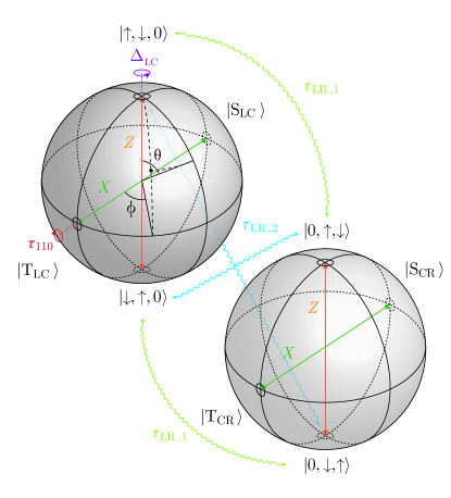
Figure 1: Scheme of the quantum state manipulation and transfer. The state is prepared in the left two-level system defined in the left and center quantum dots. Here it is represented as a Bloch sphere with angles $\theta,\phi$. The angle $\theta$ is set through the exchange interaction $\tau_{110}$, while $\phi$ is set through a magnetic field gradient between the left and center dots, $\Delta_{\mathrm{LC}}$. The prepared state is then transferred to the two-level system defined in the center and right quantum dots through the long-range photoassisted paths $\tau_{\mathrm{LR,1}}$ and ï¿œ$\tau_{\mathrm{LR,2}}$, denoted by curly arrows.

Two-electron states in two quantum dots offer a flexible and well-studied platform for quantum information purposes, forming the basis of the well-known singlet-triplet qubitHanson et al. (2007). Combining electric and magnetic control through the exchange interaction and magnetic field gradients provides full single-qubit manipulation capabilities and can be extended to include two-qubit operationsWardrop and Doherty (2014). The possibility of state transfer between spin-triplet qubits offers new possibilities for the development of new quantum architectures based on this platform. In that direction, a long-range protocol based on a singlet-triplet qubit has been proposed recentlyFeng et al. (2018) based on adiabatic transfer and Coulomb interaction engineering.

In this work we propose how to prepare a quantum state with two electrons in the left and center quantum dots of a triple quantum dot (TQD) system and how to transfer it coherently to the center and right dots by using ac gate voltages. The ac driving allows us to stop the evolution of the prepared state and to select a long range quantum transfer path. The two electrons are transferred simultaneously and coherently with high fidelity, even in the presence of charge noise. Furthermore, we develop a general transfer protocol for arbitrary gradient configurations, ensuring that our proposal can be extended to longer quantum dot arrays. The paper is organized as follows. In Section II.1 we introduce the effective Hamiltonian that we employ to study the ac response of the system. In Section II.2 we propose a transfer protocol in the case in which there are no magnetic field gradients. In Section II.3, we analyze the role of magnetic gradients in the transfer process. Finally, in Section II.4 we analyze the fidelity of the protocol under the effect of charge noise and discuss other possible sources of decoherence.

II Results

II.1 Theoretical model

We consider up to two electrons in a TQD in series. A external magnetic field produces a Zeeman splitting within each dot. Two oscillating electric field voltages are locally applied to the left and right quantum dots $H_{\text{ac}}(t)=V_{\text{ac}}^{\text{L}}\cos(\omega t)\hat{\text{n}}_{\text{L}}+V_{\text{ac}}^{\text{R}}\cos(\omega t)\hat{\text{n}}_{\text{R}}$. The Hamiltonian can be written in the interaction picture as $H_{I}(t)=\mathcal{U}_{I}(t)[H(t)-i\hbar\partial_{t}]\mathcal{U}_{I}^{\dagger}(t)$ where $\mathcal{U}_{I}(t)=\exp\left[(i/\hbar)\int H_{\mathrm{ac}}(t)dt\right]$. Then, the Hamiltonian reads

$$H_{I}(t) =\sum_{i,\sigma}\epsilon_{i}\hat{\text{c}}_{i,\sigma}^{{\dagger}}\hat{\text{c}}_{i,\sigma}+\sum_{i}B_{z,i}\hat{S}_{z,i}$$

$$+\sum_{i<j,\sigma,\sigma^{\prime}}U_{ij}\hat{n}_{i,\sigma}^{{\dagger}}\hat{n}_{j,\sigma^{\prime}}+\sum_{i}U_{ii}\hat{n}_{i,\uparrow}^{{\dagger}}\hat{n}_{i,\downarrow}$$

$$+\sum_{\sigma}\sum_{\nu=-\infty}^{\infty}t_{\text{LC}}^{\nu}(t)(\hat{c}_{\text{L},\sigma}^{{\dagger}}\hat{c}_{\text{C},\sigma}+\text{H.c.}),$$

$$+\sum_{\sigma}\sum_{\nu=-\infty}^{\infty}t_{\text{CR}}^{\nu}(t)(\hat{c}_{\text{R},\sigma}^{{\dagger}}\hat{c}_{\text{C},\sigma}+\text{H.c.})$$ (1)

where $i,j=\{\text{L,C,R}\}$ and $\sigma,\sigma^{\prime}=\{\uparrow,\downarrow\}$. The different parameters correspond to the on-site energy $\epsilon_{i}$, and the Zeeman splitting $B_{z,i}$ of the $i$th dot; the inter-dot interaction $U_{ij}$, the intra-dot interaction $U_{ii}$, and the renormalized tunnel couplings between the dots $t_{\text{LC}}^{\nu}(t)=\tau_{\text{LC}}J_{\nu}(V_{\text{ac}}^{\text{L}}/\hbar\omega)\text{e}^{i\nu\omega t}$ and $t_{\text{CR}}^{\nu}(t)=\tau_{\text{CR}}J_{\nu}(V_{\text{ac}}^{\text{R}}/\hbar\omega)\text{e}^{i\nu\omega t}$, where $J_{\nu}(\alpha)$ is the $\nu$th Bessel function of the first kind. We also denote the energy of each state as $E_{ij}=\epsilon_{i}+\epsilon_{j}+U_{ij}$. We assume a configuration where the energy differences of $\ket{\sigma,0,\sigma^{\prime}}$ and the doubly-occupied states with the states $\ket{\sigma,\sigma^{\prime},0}$ and $\ket{0,\sigma,\sigma^{\prime}}$ are the largest energy scales in the system, i.e., $\{V_{\text{ac}}^{\text{L}},V_{\text{ac}}^{\text{R}},\hbar\omega,|\tau_{ij}|,|E_{\text{LC}}-E_{\text{CR}}|,|\Delta_{ij}|\}\ll\{|\delta_{101}|,|\delta_{020}|,|\delta_{200}|,|\zeta_{101}|,|\zeta_{020}|,|\zeta_{002}|\}$, where $\delta_{101}\equiv E_{\text{LR}}-E_{\text{LC}}$, $\delta_{020}\equiv E_{\text{CC}}-E_{\text{LC}}$, $\delta_{200}\equiv E_{\mathrm{LL}}-E_{\mathrm{LC}}$, $\zeta_{101}\equiv E_{\text{LR}}-E_{\text{CR}}$, $\zeta_{020}\equiv E_{\text{CC}}-E_{\text{CR}}$, $\zeta_{002}\equiv E_{\mathrm{RR}}-E_{\mathrm{CR}}$ and $\Delta_{ij}=(B_{z,j}-B_{z,i})/2$. In this regime we obtain an effective Hamiltonian with virtual tunneling as the leading order of perturbation by means of a time-dependent Schrieffer-Wolff transformationGoldin and Avishai (2000). Written in the basis $\{\ket{\uparrow,\downarrow,0},\ket{\downarrow,\uparrow,0},\ket{0,\uparrow,\downarrow},\ket{0,\downarrow,\uparrow}\}$, the effective Hamiltonian reads

$$H_{\mathrm{eff}}(t)=\left[\begin{array}[]{cccc}\tilde{E}_{|\uparrow,\downarrow,0\mathcal{i}}(t)&\tau_{110}^{*}(t)&\tau_{\mathrm{LR,1}}^{*}(t)&\tau_{\mathrm{LR,2}}^{*}(t)\\ \tau_{110}(t)&\tilde{E}_{|\downarrow,\uparrow,0\mathcal{i}}(t)&\tau_{\mathrm{LR,2}}^{*}(t)&\tau_{\mathrm{LR,1}}^{*}(t)\\ \tau_{\mathrm{LR,1}}(t)&\tau_{\mathrm{LR,2}}(t)&\tilde{E}_{|0,\uparrow,\downarrow\mathcal{i}}(t)&\tau_{011}^{*}(t)\\ \tau_{\mathrm{LR,2}}(t)&\tau_{\mathrm{LR,1}}(t)&\tau_{011}(t)&\tilde{E}_{|0,\downarrow,\uparrow\mathcal{i}}(t)\end{array}\right].$$ (2)

$\tilde{E}_{k}(t)$ are the renormalized energies of the states, $\tau_{110}(t)$ and $\tau_{011}(t)$ are the rates for the exchange interactions due to virtual transitions through the doubly occupied states $\ket{\uparrow\downarrow,0,0},\ket{0,\uparrow\downarrow,0}$ and $\ket{0,0,\uparrow\downarrow}$. $\tau_{\mathrm{LR,1}}(t)$ and $\tau_{\mathrm{LR,2}}(t)$ are the amplitudes for the long-range processes connecting $\{\ket{\uparrow,\downarrow,0},\ket{\downarrow,\uparrow,0}\}$ and $\{\ket{0,\uparrow,\downarrow},\ket{0,\downarrow,\uparrow}\}$ by virtual transitions through the $\ket{0,\uparrow\downarrow,0}$ and $\ket{\sigma,0,\sigma^{\prime}}$ states. The expressions for the different terms in the effective Hamiltonian are given in the Supplementary information.

The proposed protocol consists of the preparation of a state

$$|\Psi_{\mathrm{L}}\mathcal{i}=\cos(\theta_{\mathrm{L}}/2)\ket{\uparrow,\downarrow,0}+e^{i\phi_{\mathrm{L}}}\sin(\theta_{\mathrm{L}}/2)\ket{\downarrow,\uparrow,0}$$ (3)

in the two-level system $\mathcal{Q}_{\mathrm{L}}=\{\ket{\uparrow,\downarrow,0},\ket{\downarrow,\uparrow,0}\}$ defined in the left and center dots, where $\phi_{\mathrm{L}}$ can be defined in terms of the density matrix $\rho$ as

$$\phi_{\text{L}}=\text{Arg}\left[\frac{\braket{\uparrow,\downarrow,0}{\rho}{\downarrow,\uparrow,0}}{\sqrt{\braket{\uparrow,\downarrow,0}{\rho}{\uparrow,\downarrow,0}\braket{\downarrow,\uparrow,0}{\rho}{\downarrow,\uparrow,0}}}\right],$$ (4)

Manipulation of both $\theta_{\mathrm{L}}$ and $\phi_{\mathrm{L}}$ is attained by a combination of the magnetic field gradients and the exchange interaction due to virtual processes involving the doubly occupied states, with corresponding transition rates $\tau_{110}(t)$ and $\tau_{011}(t)$. Then, the prepared state can be transferred to the two-level system $\mathcal{Q}_{\mathrm{R}}=\{\ket{0,\uparrow,\downarrow},\ket{0,\downarrow,\uparrow}\}$ defined in the center and right dots, yielding

$$\ket{\psi_{\mathrm{R}}}=\cos(\theta_{\mathrm{L}}/2)\ket{0,\uparrow,\downarrow}+e^{i\phi_{\mathrm{L}}}\sin(\theta_{\mathrm{L}}/2)\ket{0,\downarrow,\uparrow}.$$ (5)

This transfer is carried out through the long-range photoassisted paths, with rates given by $\tau_{\mathrm{LR,1}}(t)$ and $\tau_{\mathrm{LR,2}}(t)$. The former, $\tau_{\mathrm{LR,1}}(t)$, connects states in the same poles of the Bloch sphere, while the latter, $\tau_{\mathrm{LR,2}}(t)$ connects states in opposite poles of the sphere (see Fig. 1). Two problems arise from this configuration. First, the exchange interactions act on the quantum state during the transfer. Second, there are two different transference channels, which limits the fidelity. Both can be solved by using ac-driving fields. By choosing the proper ac-driving amplitudes, the interference between the different photoassisted paths with rates $\tau_{110}(t),\tau_{011}(t),$ and $\tau_{\mathrm{LR,2}}(t)$ can be used to nullify these processes, as will be shown below.

We consider in Sec. II.2 the simpler case in which there are no magnetic field gradients. Then, we will consider the general case with arbitrary magnetic field gradients in Sec. II.3.

II.2 Without magnetic field gradients

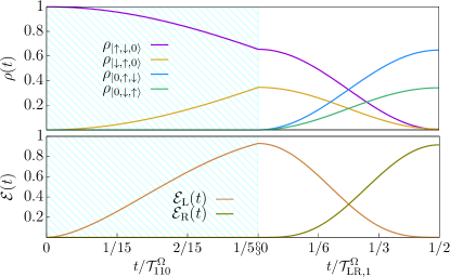
Figure 2: (top) Time evolution of the population of the different states. (bottom) Time evolution of the entanglement between the spins. The two spins in $\mathcal{Q}_{\mathrm{L}}$ are prepared into an state $|\Psi_{\mathrm{L}}\mathcal{i}=\cos(\theta_{\mathrm{L}}/2)\ket{\uparrow,\downarrow,0}+e^{i\phi_{\mathrm{L}}}\sin(\theta_{\mathrm{L}}/2)\ket{\downarrow,\uparrow,0}$ with $\theta_{\text{L}}=2\pi/5$ and $\phi_{\mathrm{L}}=\pi/2$ by means of $\tau_{110}$ (dashed green area) and then the state is transferred to $\mathcal{Q}_{\mathrm{R}}$ (white area). Parameters: $\tau_{\text{LC}}=\tau_{\text{CR}}=\tau=30\mu\text{eV}$, $\epsilon_{\text{C}}/\omega=6.48$, $\tilde{E}_{\text{LC}}=0$ and $\tilde{E}_{\text{CR}}=\omega$. In the left part of the figure (blue dashed area) the ac gate voltages are switched off. In the right part of the figure: $V_{\text{ac}}^{\text{L}}=3.94\mu\text{eV}$ and $V_{\text{ac}}^{\text{R}}=3.57\mu\text{eV}$, $\omega=10\tau$.

Our first protocol consists on preparing a quantum state in $\mathcal{Q}_{\mathrm{L}}$ allowing only $\theta_{\mathrm{L}}$ to evolve (see Eq. 3) and then transferring it to $\mathcal{Q}_{\mathrm{R}}$. The procedure can be fashioned as an entanglement generation between the single spins in $\mathcal{Q}_{\mathrm{L}}$ dots and a transfer of the entangled spins to $\mathcal{Q}_{\mathrm{R}}$. Initially, we turn the ac voltages off and assume that there is no charge transfer between $\mathcal{Q}_{\mathrm{L}}$ and $\mathcal{Q}_{\mathrm{R}}$. Under the assumptions leading to Eq. 2, this requires that the energy difference between the states in $\mathcal{Q}_{\mathrm{L}}$ and $\mathcal{Q}_{\mathrm{R}}$ is much larger than the amplitudes of the long-range rates $\tau_{\mathrm{LR,1}}$ and $\tau_{\mathrm{LR,2}}$.

The initial state is taken as $\ket{\uparrow,\downarrow,0}$. The desired value of $\theta_{\mathrm{L}}$ can be set by allowing the system to evolve by means of the virtual transitions with the doubly occupied states $\ket{\uparrow\downarrow,0,0}$ and $\ket{0,\uparrow\downarrow,0}$ through $\tau_{110}$, yielding the state $|\Psi_{\mathrm{L}}\mathcal{i}=\cos(\theta_{\mathrm{L}}/2)\ket{\uparrow,\downarrow,0}+e^{i\pi/2}\sin(\theta_{\mathrm{L}}/2)\ket{\downarrow,\uparrow,0}$. With the ac voltages turned off, $\tau_{110}$ is given by

$$\tau_{110} =-\frac{\tau_{\mathrm{LC}}^{2}}{2}\left(\frac{1}{\delta_{200}}+\frac{1}{\delta_{020}}\right)$$ (6)

This process has a Rabi period $\mathcal{T}_{110}^{\Omega}=\pi\hbar/|\tau_{110}|$ which can be controlled either by modifying the detuning between the left and center dots (i.e: controlling $\delta_{020}$) or by symmetric control of the tunneling barriersRuss and Burkard (2017) (i.e: controlling $\tau_{\mathrm{LC}}$). The latter method has the benefit of allowing for operation under the sweetspot conditionFei et al. (2015); Martins et al. (2016), resulting in lower sensitivity to charge noise.

Once the spins are in the desired state, the ac voltages are turned on and the state is transferred to the center and right dots. With the ac voltages on, the diagonal terms of Eq. 2 are time-dependent. To obtain the resonance condition that allows us to transfer the state, we calculate the mean in time of the diagonal terms, the mean energies. These can be obtained as

$$\tilde{E}_{\mathrm{LC}} =E_{\mathrm{LC}}$$

$$-\sum_{\nu}\left[\frac{|t_{\mathrm{CR}}^{\nu}|^{2}}{\delta_{101}+\nu\hbar\omega}+\frac{|t_{\mathrm{LC}}^{\nu}|^{2}}{\delta_{020}-\nu\hbar\omega}+\frac{|t_{\mathrm{LC}}^{\nu}|^{2}}{\delta_{200}-\nu\hbar\omega}\right]$$ (7)

$$\tilde{E}_{\mathrm{CR}} =E_{\mathrm{CR}}$$

$$-\sum_{\nu}\left[\frac{|t_{\mathrm{LC}}^{\nu}|^{2}}{\zeta_{101}+\nu\hbar\omega}+\frac{|t_{\mathrm{CR}}^{\nu}|^{2}}{\zeta_{020}-\nu\hbar\omega}+\frac{|t_{\mathrm{CR}}^{\nu}|^{2}}{\zeta_{002}-\nu\hbar\omega}\right]$$ (8)

Here $\nu$ is the sideband index and goes from $-\infty$ to $\infty$ unless explicitly noted. Then, we assume that the difference between the mean energies of the initial (left) and final (right) states is $n\hbar\omega$. If $n=0$, the tunnel barrier between the center and right dots has to be raised so that $\tau_{\mathrm{CR}}\simeq 0$ while preparing the state avoiding electron transfer to the rightmost dot. During the transfer, the tunnel barriers are then lowered to allow the electrons to tunnel to the center and right dots. If $n\neq 0$ and $\omega\gg\tau_{\mathrm{LC}},\tau_{\mathrm{CR}}$, $\mathcal{Q}_{\mathrm{L}}$ and $\mathcal{Q}_{\mathrm{R}}$ will only be coupled when the ac field is turned on. This eliminates the need to manipulate the tunnel amplitudes for the state transfer.

When the resonance condition $|\tilde{E}_{\mathrm{CR}}-\tilde{E}_{\mathrm{LC}}|=n\hbar\omega$, $n\mathcal{2}\mathbb{N}$ is met, we can use the rotating wave approximation (RWA), in which the energies of the Hamiltonian are shifted to the desired resonance and the fast oscillating terms are neglected. For that we apply a unitary transformation: $\mathcal{U}_{\mathrm{RWA}}^{{\dagger}}(t)[H_{\text{eff}}(t)-i\hbar\partial_{t}]\mathcal{U}_{\mathrm{RWA}}(t)$ where $\mathcal{U}_{\mathrm{RWA}}(t)=\exp\left[-in\omega t(\hat{n}_{\ket{0,\uparrow,\downarrow}}+\hat{n}_{\ket{0,\downarrow,\uparrow}})\right]$. This allows to obtain time-independent rates for the second order processes, as given in the Supplementary information. Unless explicitly noted, the formulas in the next sections are obtained from the RWA approximation.

During the transfer process, the energy levels of $\ket{\uparrow,\downarrow,0}$ and $\ket{\downarrow,\uparrow,0}$ are resonant and virtual transitions between the two states through the double occupied states modify $\theta_{\text{L}}$. The formation of a dark state is required in order to stop the evolution of $\theta_{\text{L}}$. Only if the state is a singlet or a triplet, the state is an eigenstate of the exchange Hamiltonian, $\theta_{\mathrm{L}}$ does not change during the transfer process and ac fields are not required to stop the evolution of $\theta_{\mathrm{L}}$. For a general state, destructive interferences between the virtual photoassisted paths may lead to $\tau_{110}^{\text{RWA}}=0$. This occurs for values of the driving amplitude $V_{\text{ds}}^{\text{L}}$ such that

$$\sum_{\nu}J_{\nu}^{2}\left(\frac{V_{\text{ds}}^{\text{L}}}{\hbar\omega}\right)\left(\frac{1}{\delta_{020}-\nu\hbar\omega}+\frac{1}{\delta_{200}-\nu\hbar\omega}\right)=0$$ (9)

Hence, the time evolution of $\theta_{\text{L}}$ can be stopped at any desired point through the ac gates by setting $V_{\text{ac}}^{\text{L}}=V_{\text{ds}}^{\text{L}}$. Similarly, for $\mathcal{Q_{\mathrm{R}}}$, a similar dark state condition can be obtained for an ac driving amplitude $V_{\text{ac}}^{\text{R}}=V_{\text{ds}}^{\text{R}}$.

There are two possible transport channels between $\mathcal{Q}_{\mathrm{L}}$ and $\mathcal{Q}_{\mathrm{R}}$ (see Fig. 1), controlled by the virtual tunneling couplings $\tau_{\mathrm{LR,1}}^{n}$ and $\tau_{\mathrm{LR,2}}^{n}$Note (1). Only if the state is a triplet, transitions through the singlet $\ket{0,\uparrow\downarrow,0}$ are forbidden and $\tau_{\mathrm{LR,2}}^{n}=0$ always. For a general state, the simultaneous presence of the two channels limits the fidelity of the transfer process and the transition rate corresponding to one of the long range photo-assisted paths, either $\tau_{\text{LR},1}^{n}$ or $\tau_{\text{LR},2}^{n}$, has to be set to zero. The ac voltage can induce a destructive interference between the sidebands and nullify $\tau_{\mathrm{LR,1}}^{n}$ or $\tau_{\mathrm{LR,2}}^{n}$ in the same way as for $\tau_{110}$ and $\tau_{011}$. For concreteness, we consider transfer between $\mathcal{Q}_{\mathrm{L}}$ and $\mathcal{Q_{\mathrm{R}}}$ just through $\tau_{\text{LR},1}^{n}$. Then, $\tau_{\text{LR},2}^{n}$ is suppressed for a set of values

$$\epsilon_{\text{C}}^{\text{ds}}=\left\{\epsilon_{\text{C}}\ \big{|}\ \tau_{\text{LR},2}^{n}=0\ \&\ \tau_{\text{LR},1}^{n}\neq 0\right\},$$ (10)

where $\epsilon_{\text{C}}^{\text{ds}}$ is the energy of the central level at which the destructive interference between the virtual photon-sidebands occurs and $\tau_{\text{LR},2}^{n}=0$. In Fig. 2 we have plotted the occupation of the relevant states and the entanglement of the two spins during the preparation and transfer protocol. In the blue dashed area, $\theta_{\mathrm{L}}$ is fixed by letting the state evolve under $\tau_{110}$ for a certain time, with the ac voltages turned off. Then, the ac voltages are turned on, connecting $\mathcal{Q}_{\mathrm{L}}$ to $\mathcal{Q}_{\mathrm{R}}$. In the white area, the state is transferred through the $\tau_{\mathrm{LR,1}}^{n}$ process from $\mathcal{Q}_{\mathrm{L}}$ to $\mathcal{Q}_{\mathrm{R}}$.

II.3 With magnetic field gradients

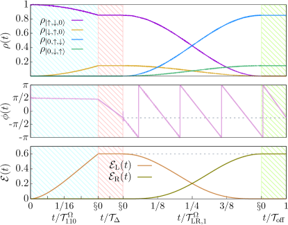
Figure 3: For $\Delta_{\mathrm{LC}}=\Delta_{\mathrm{CR}}$. (top) Time evolution of the population of the states. (center) Time evolution of $\phi(t)$. The phase $\phi(t)$ is defined in $\mathcal{Q}_{\mathrm{L}}$ during the manipulation process and in $\mathcal{Q}_{\mathrm{R}}$ during the transfer process. (bottom) Time evolution of the entanglement $\mathcal{E}(t)$ between the two spins. From left to right: in the blue dashed area $\theta_{\mathrm{L}}$ is fixed to the desired value of $\theta_{\mathrm{L}}=\pi/4$; in the red dashed area the polar angle $\phi_{\mathrm{L}}=-\pi/4$ is set through the magnetic field gradient while $\tau_{110}\simeq 0$; in the white area the two tunnel barriers are lowered and the state is transferred through $\tau_{\mathrm{LR,1}}$; in the green dashed area the phase is corrected to its value of $\phi_{\mathrm{L}}=-\pi/4$. Parameters: $\Delta_{\mathrm{LC}}=\Delta_{\mathrm{CR}}=0.13$ $\mathrm{\mu eV}$. $\tau_{\mathrm{LC}}=\tau_{\mathrm{CR}}=30$ $\mathrm{\mu eV}$ in the white areas and the blue dashed areas and $\tau_{\mathrm{LC}}=\tau_{\mathrm{CR}}=0$ in the red and green dashed areas. $\delta_{020}=\zeta_{020}=4.25$ meV, $\delta_{101}=\zeta_{101}=2.28$ meV, $n=0$. In the dashed areas the ac gate voltages are switched off. In the right part of the figure (white areas): $V_{\text{ac}}^{\text{L}}=V_{\mathrm{ac}}^{\mathrm{L}}=5.25\,\text{meV}$ $\omega=0.5$ $\mathrm{meV}$. The gray dashed lines are a visual guide indicating the desired value of $\phi$ and the entanglement of the initially prepared state.

A magnetic field gradient, produced for instance by nanomagnetsPetersen et al. (2013); Forster et al. (2015); Yoneda et al. (2015), allows for the generation of any state in $\mathcal{Q}_{\mathrm{L}}$. As long as $|\delta_{101}|,|\delta_{020}|,|\delta_{200}|\gg\tau_{\mathrm{LC}}$, leakage into the $\ket{\sigma,0,\sigma^{\prime}},\ket{\uparrow\downarrow,0,0}$ and $\ket{0,\uparrow\downarrow,0}$ states can be kept minimal. At this point, the TQD operates as a two-level system $\{\ket{\uparrow,\downarrow,0},\ket{\downarrow,\uparrow,0}\}$ with Hamiltonian

$$H_{\mathrm{LC}}=-\Delta\tilde{E}_{\mathrm{LC}}\hat{\sigma}_{\mathrm{LC}}^{z}+\tau_{110}\hat{\sigma}_{\mathrm{LC}}^{x},$$ (11)

with $\hat{\sigma}_{\mathrm{LC}}^{i}$ the $i$th Pauli matrix in $\mathcal{Q}_{\mathrm{L}}$, $i=x,z$ and

$$\Delta\tilde{E}_{\mathrm{LC}}=\frac{1}{2}\left(\tilde{E}_{|\downarrow,\uparrow,0\mathcal{i}}-\tilde{E}_{|\uparrow,\downarrow,0\mathcal{i}}\right).$$ (12)

The ground state for $\tau_{110}\simeq 0$ is given by $\ket{\uparrow,\downarrow,0}$ due to the magnetic field gradient. This state, located in the north pole of the Bloch sphere depicted in Fig. 1 only acquires a global phase as a result of the gradient, therefore providing a suitable platform for initialization. The desired state is then prepared starting from $\ket{\uparrow,\downarrow,0}$ by a combination of the magnetic field gradient and the exchange interaction $\tau_{110}$Hanson et al. (2007); Hanson and Burkard (2007). A single rotation is enough to yield any state with $\theta\leq\theta_{\mathrm{max}}$, where $\theta_{\mathrm{max}}=2\arcsin\left(|\tau_{110}|/\sqrt{\tau_{110}^{2}+\Delta\tilde{E}_{\mathrm{LC}}^{2}}\right)$. For states with $\theta>\theta_{\mathrm{max}}$, an arbitrary $X$ axis rotation can be realized by applying three consecutive rotationsHanson and Burkard (2007). If $\theta\leq\theta_{\mathrm{max}}$, the system acquires a finite phase $\phi^{\prime}$ while setting $\theta_{\mathrm{L}}$. Then, a second, independent axis of control is given by raising the barriers, so that $\tau_{110}\simeq 0$. This yields a rotation around the $Z$ axis, which can be used to set the desired value of $\phi_{\mathrm{L}}$ by letting the system evolve for a fraction of the period $\mathcal{T}_{\Delta}=\pi\hbar/|\Delta_{\mathrm{LC}}|$.

As in Sec. II.2, the quantum state transfer is initiated by turning the ac voltage on. As before, $\tau_{110}$ needs to be set to zero so that $\theta_{\mathrm{L}}$ does not vary during the transfer process. In the presence of gradients, the dark state condition leading to $\tau_{110}=0$ is given by

$$\sum_{\nu}J_{\nu}^{2}\left(\frac{V_{\text{ds}}^{\text{L}}}{\hbar\omega}\right)\left[\frac{1}{\delta_{020}+\Delta_{\mathrm{LC}}-\nu\hbar\omega}+\frac{1}{\delta_{200}+\Delta_{\mathrm{LC}}-\nu\hbar\omega}\right.$$

$$\left.+\frac{1}{\delta_{020}-\Delta_{\mathrm{LC}}-\nu\hbar\omega}+\frac{1}{\delta_{200}-\Delta_{\mathrm{LC}}-\nu\hbar\omega}\right]=0$$

and similar conditions can be obtained for $\tau_{011}$ and $\tau_{\mathrm{LR,}2}^{n}$. Furthermore, we will assume that $|\Delta_{\mathrm{LC}}-\Delta_{\mathrm{CR}}|\ll\omega$ so that the RWA approximation holds.

The procedure for transferring the state from one edge to the other depends on the gradient configuration. If the magnetic field gradients are much smaller than the long-range transfer rate $\tau_{\mathrm{LR},1}^{n}$, the state can be transferred directly without significant variation in $\phi_{\mathrm{L}}$, following the same protocol as in the case without magnetic gradients. Otherwise, two problems arise. First, the finite gradient results in a change in $\phi_{\mathrm{L}}$ during the transfer process. This can be circumvented by letting $\phi_{\mathrm{L}}$ evolve during a finite time after the transfer process is finished in order to compensate the change in $\phi_{\mathrm{L}}$. The second problem is the difference between the gradients in $\mathcal{Q}_{\mathrm{L}}$ and $\mathcal{Q}_{\mathrm{R}}$, which imposes a limit to the fidelity of a transfer process (through the long-range channel $\tau_{\mathrm{LR,1}}^{n}$) that can be estimated asNote (1)

$$\mathcal{F}_{\mathrm{max}}\simeq 1-\frac{|\Delta_{\mathrm{CR}}-\Delta_{\mathrm{LC}}|}{\sqrt{\left(\Delta_{\mathrm{CR}}-\Delta_{\mathrm{LC}}\right)^{2}+\left(2\tau_{\mathrm{LR,1}}^{n}\right){}^{2}}}.$$ (13)

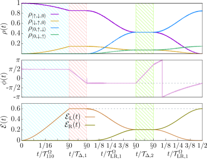
Figure 4: For $\Delta_{\mathrm{LC}}=-\Delta_{\mathrm{CR}}$: (top) Time evolution of the population of the states. (center) Time evolution of $\phi(t)$. The phase $\phi(t)$ is defined in $\mathcal{Q}_{\mathrm{L}}$ during the manipulation process and in $\mathcal{Q}_{\mathrm{R}}$ during the transfer process. (bottom) Time evolution of the entanglement $\mathcal{E}(t)$ between the two spins. From left to right: in the blue dashed area $\theta_{\mathrm{L}}$ is fixed to the desired value of $\theta_{\mathrm{L}}=\pi/4$; in the red dashed area the polar angle $\phi_{\mathrm{L}}=-\pi/4$ is set through the magnetic field gradient while $\tau_{110}\simeq 0$; in the first white area, the state is transferred to a superposition with equal weight in $\mathcal{Q}_{\mathrm{L}}$ and $\mathcal{Q}_{\mathrm{R}}$; in the green area, the system is left to evolve under the gradients, $\Delta_{\mathrm{LC}}$ and $\Delta_{\mathrm{CR}}$, for a time $\mathcal{T}_{\Delta}/2=\pi/2|\Delta_{\mathrm{LC}}|$; finally, in the second white area, the state is transferred from the superposition between $\mathcal{Q}_{\mathrm{L}}$ and $\mathcal{Q}_{\mathrm{R}}$ to $\mathcal{Q_{\mathrm{R}}}$. Parameters: $\Delta_{\mathrm{LC}}=-\Delta_{\mathrm{CR}}=\tau_{\text{LR,1}}$. $\tau_{\mathrm{LC}}=\tau_{\mathrm{CR}}=30$ $\mathrm{\mu eV}$ in the white areas and the blue dashed areas and $\tau_{\mathrm{LC}}=\tau_{\mathrm{CR}}=0$ in the red and green dashed areas. , $\delta_{020}=\zeta_{020}=4.25$ meV, $\delta_{101}=\zeta_{101}=2.28$ meV, $n=0$. In the dashed areas the ac gate voltages are switched off. In the white areas: $\omega=0.5$ $\mathrm{meV}$ and $V_{\text{ac}}^{\text{L}}=V_{\mathrm{ac}}^{\mathrm{L}}=5.25\,\text{meV}$. The gray dashed lines are a visual guide indicating the desired value of $\phi$ and the entanglement of the initially prepared state.

We consider first the simpler case of $\Delta_{\mathrm{LC}}=\Delta_{\mathrm{CR}}=\Delta$ (the linear configuration). The estimated maximum fidelity, Eq. 13 is 1 for this configuration. Hence, the only issue with the presence of the gradients in this configuration is that the phase $\phi_{\mathrm{L}}$ keeps evolving during the state transfer. This can be circumvented by letting the phase evolve for a time

$$\mathcal{T}_{\mathrm{off}}=\left[N\mathcal{T}_{\Delta}-\mathcal{T}_{\mathrm{LR,1}}^{\Omega}/2\right],\,\,\,N\mathcal{2}\mathbb{Z}$$ (14)

once the state has been transferred, where

$$\mathcal{T}_{\mathrm{LR,1}}^{\Omega}=2\pi\hbar\left[\left(2\tau_{\mathrm{LR,1}}^{n=0}\right)^{2}+\left(\Delta_{\mathrm{LC}}-\Delta_{\mathrm{CR}}\right)^{2}\right]^{-1/2}.$$ (15)

is the Rabi period corresponding to $\tau_{\text{LR,1}}^{n=0}$, written here for arbitrary $\Delta_{\text{LC}},\Delta_{\text{CR}}$ for completeness. $\mathcal{T}_{\mathrm{off}}$ does not depend on the particular state being transferred and in that sense the process is still universal. The process is illustrated in Fig. 3. Initially, we set $\tau_{\mathrm{CR}}=0$ since the levels are not detuned; in the blue dashed part, $\theta_{\mathrm{L}}$ is fixed to its desired value of $\pi/4$ through $\tau_{110}$. Note that $\tau_{110}\gg\Delta_{\mathrm{LC}}$, and therefore $\phi^{\prime}\simeq\pi/2$ when $\theta_{\mathrm{L}}$ reaches $\pi/4$. In the red dashed area, we set $\tau_{110}=0$ and the phase evolves from $\phi^{\prime}$ to $\phi_{\mathrm{L}}$ (marked by a gray dashed line). Then, the two barriers are lowered and the transfer process is carried out for a time $\mathcal{T}_{\mathrm{LR,1}}^{\Omega}/2$. Finally, in the green dashed area, the barriers are raised again and the phase $\phi_{\mathrm{L}}$ is left to evolve for a time $\mathcal{T}_{\mathrm{off}}$ until the desired value $\phi_{\mathrm{L}}$ is reached.

If $\Delta_{\mathrm{LC}}\neq\Delta_{\mathrm{CR}}$, the maximum fidelity, Eq. 13, cannot reach 1 for a transfer operation in a single step. Hence, there are two options to transfer the state: (i) if the difference between the gradients is much smaller than the long-range transition rates, $\left|\Delta_{\mathrm{LC}}-\Delta_{\mathrm{CR}}\right|\ll\left|\tau_{\mathrm{LR,1}}^{n}\right|$, and so $\mathcal{F}_{\mathrm{max}}\simeq 1$ for a single transfer operation; (ii) a combination of operations in one of the two level systems $\mathcal{Q}_{\mathrm{L}}$ and $\mathcal{Q}_{\mathrm{R}}$ and transfer operations through $\tau_{\mathrm{LR,1}}^{n}$ is used to ensure an ideal 100% fidelity at the cost of longer transfer times. The latter case is discussed in detail in the Supplementary Information and a universal transfer process with 100% fidelity for any $\{\Delta_{\mathrm{LC}},\Delta_{\mathrm{CR}}\}$ configuration is proposed.

Here, we consider for example $\Delta_{\mathrm{LC}}=-\Delta_{\mathrm{CR}}$ in Fig. 4 (the symmetric configuration). This configuration has the particularity that $\phi_{\mathrm{L}}$ is not modified during a single transfer process, as can be seen in the first white section of Fig. 4 (center). On the other hand, the maximum fidelity of a single transfer operation, as given in Eq. 13, is minimal for this configuration. To transfer the state with 100% ideal fidelity, a sequence consisting of (i) transfer from $\mathcal{Q_{\mathrm{L}}}$ to a superposition of the desired state with equal weight in $\mathcal{Q}_{\mathrm{L}}$ and $\mathcal{Q}_{\mathrm{R}}$, (ii) evolution under the gradients, $\Delta_{\mathrm{LC}}$ and $\Delta_{\mathrm{CR}}$, for a time $\mathcal{T}_{\Delta}/2=\pi\hbar/\left(2|\Delta_{\mathrm{LC}}|\right)$ and (iii) another transfer process as in (i) from the superposition between $\mathcal{Q}_{\mathrm{L}}$ and $\mathcal{Q}_{\mathrm{R}}$ to $\mathcal{Q}_{\mathrm{R}}$, can be used to transfer the state with maximum fidelity. The operations (i)-(iii) correspond to the first white area, the green dashed area and the second white area of Fig. 4, respectively. Each of the transfer operations, (i) and (iii) is carried out for a time $\mathcal{T}_{\mathrm{LR,1}}^{\Omega}/2$.

If the magnetic field gradients could be be switched off rapidly enough during operation, the transfer protocol could be performed in the simpler manner of Section II.2 (i.e. independent of the gradient configuration). This has been recently shown to be possible in reasonable operation timesBodenstedt et al. (2018).

II.4 Relaxation and decoherence

In this section we will discuss the effect of relaxation and decoherence on the protocol. There are several possible sources of decoherence in these systems, but the most important is the coupling to charge noise. We will discuss charge noise first and later on we will consider other sources of decoherence. For charge noise we will search for optimal operation points (sweetspots) under which the coupling to charge noise is minimized.

II.4.1 Charge noise

In order to estimate the effect of charge noise we consider that the system is coupled to a bath consisting of a set of independent harmonic oscillators. The Hamiltonian for the system and bath is given by $H=H_{\mathrm{S}}(t)+H_{\mathrm{B}}+H_{\mathrm{SB}}$, where $H_{\mathrm{S}}(t)$ is the Hamiltonian for the system as given by Eq. 2 and

$$H_{\mathrm{B}} =\sum_{i,n}\hbar\omega_{n}\hat{b}_{i,n}^{\dagger}\hat{b}_{i,n}$$ (16)

$$H_{\mathrm{SB}} =\sum_{i}X_{i}\xi_{i}=\sum_{i,n}g_{n}X_{i}(\hat{b}_{i,n}^{\dagger}+\hat{b}_{i,n})$$ (17)

$\{X_{i}\}$ is the set of system operators coupled to the bath. In our case we consider only charge noise, corresponding to $X_{i}=\hat{c}_{i}^{\dagger}\hat{c}_{i}$. We assume that all oscillators are equal and independent. For the bath coordinates $\{\xi_{i}\}$ this requires that the symmetrically ordered autocorrelation function satisfies $(1/2)\mathcal{h}\left\{\xi_{i}(\tau),\xi_{i}(0)\right\}\mathcal{i}=2\delta(t-t^{\prime})\delta_{ij}$. Current noise has a small effect in quantum dot-based quantum information devicesRuss and Burkard (2017) and we will not consider it here. The bath is characterized by the spectral density, $\mathcal{J}(\omega)=\pi\sum_{n}|g_{n}|^{2}\delta(\omega-\omega_{n})$, and by $\mathcal{S}(\omega)=\mathcal{J}(\omega)\mathrm{coth}(\beta\hbar\omega/2)$, the Fourier transform of the symmetrically ordered equilibrium autocorrelation function.

The system under the presence of charge noise can be studied under a Bloch-Redfield type master equationRedfield (1957); Kohler and Hänggi (2006); Qi et al. (2017). For the $1/f$ noise typically considered in quantum dot systems, the validity of the Markovian approximation inherent in a master equation approach is only warranted for weak coupling. At this level of approximation, $1/f$ noise can be considered by taking $\mathcal{J}\left(\omega\right)\simeq\text{constant}$, which gives $\mathcal{S}\left(\omega\right)\sim 1/\omega$ for $\beta\hbar\omega\ll 1$. Since $\mathcal{S}\left(\omega\right)$ diverges for low frequencies, we regularize it below a certain cutoff frequency $\omega_{\text{IR}}$ as

$$\mathcal{S}\left(\omega\right)=\begin{cases}\mathcal{S}_{0}&\omega\leq\omega_{\text{IR}}\\ \mathcal{S}_{0}\frac{\tanh\left(\beta\hbar\omega_{\text{IR}}/2\right)}{\tanh\left(\beta\hbar\omega/2\right)}&\omega>\omega_{\text{IR}}\end{cases}$$ (18)

The parameter $\mathcal{S}_{0}$ determines the dephasing time, and thus provides a natural parameter to characterize the noise intensity. We will consider the effect of noise in the protocol both for the process of manipulation and transfer.

Charge noise comes from fluctuations on the energy levels. During the manipulation process, it modifies the renormalized splitting $\Delta\tilde{E}_{\mathrm{LC}}$, given by Eq. 12 (with $V_{\mathrm{L}}^{\mathrm{ac}}=V_{\mathrm{R}}^{\mathrm{ac}}=0$), and the transition rate $\tau_{110}$, given by Eq. 6, associated to the exchange interaction. The system is effectively subjected to a single noise source $\xi_{\mathrm{LC}}=\xi_{\mathrm{C}}-\xi_{\mathrm{L}}$. Defining $\tau_{110}^{(1)}\equiv\left.\partial_{\epsilon_{\mathrm{L}}}\tau_{110}\right|_{\xi_{\mathrm{LC}}=0}$, and $\Delta\tilde{E}_{\mathrm{LC}}^{(1)}=\left.\partial_{\epsilon_{\mathrm{L}}}\Delta\tilde{E}_{\mathrm{LC}}\right|_{\xi_{\mathrm{LC}}=0}$, under the conditions $\tau_{110}^{(1)}=0$ and $\Delta\tilde{E}_{\mathrm{LC}}^{(1)}=0$, the system is unaffected by charge noise, yielding the previously mentioned sweetspotFei et al. (2015); Martins et al. (2016). The non-linear terms are only predominant at the sweetspot, but their treatment is complexMakhlin and Shnirman (2004) and we will not consider them any further. The condition $\tau_{110}^{(1)}=0$ implies that

$$\epsilon_{\mathrm{C}}-\epsilon_{\mathrm{L}}=\frac{U_{\mathrm{LL}}-U_{\mathrm{CC}}}{2}.$$ (19)

At the sweetspot, the transition rate $\tau_{110}$ is given by

$$\tau_{110} =-\tau_{\mathrm{LC}}^{2}\left(\frac{1}{\delta_{\mathrm{ss}}+\Delta_{\mathrm{LC}}}+\frac{1}{\delta_{\mathrm{ss}}-\Delta_{\mathrm{LC}}}\right)$$

where $\delta_{\mathrm{ss}}=(U_{\mathrm{LL}}+U_{\mathrm{CC}})/2-U_{\mathrm{LC}}$. Under the sweetspot condition, Eq. 19, $\Delta\tilde{E}_{\mathrm{LC}}^{(1)}=0$ as long as

$$\tau_{\mathrm{CR}}^{2}\left(\frac{1}{\delta_{101}+\Delta_{\mathrm{CR}}}-\frac{1}{\delta_{101}-\Delta_{\mathrm{CR}}}\right)=0$$ (20)

which is satisfied for $\tau_{\text{CR}}=0$ or $\Delta_{\text{CR}}=0$. The sweetspot for manipulation in $\mathcal{Q}_{\mathrm{R}}$ can be obtained in the same manner.

During the transfer process, the system couples to charge noise through several processes:

1. Direct coupling to charge noise through the energy levels of the quantum dots ($\epsilon_{\mathrm{L}},\epsilon_{\mathrm{C}},\epsilon_{\mathrm{R}}$). The system-bath interaction for this process is given by

   $$H_{\mathrm{SB,dir}}=\sum_{i}\xi_{i}\hat{c}_{i}^{\dagger}\hat{c}_{i}$$ (21)

2. Through the energy-dependence of the long-range amplitude $\tau_{\mathrm{LR,1}}$. The related relaxation and dephasing rates are proportional to the first derivative of $\tau_{\mathrm{LR,1}}$ with respect to the gate energy $\epsilon_{\mathrm{L}}$ (or $\epsilon_{\mathrm{R}}$), denoted by $\tau_{\mathrm{LR,1}}^{(1)}$.

3. Because charge noise disrupts the dark state condition and results in non-zero values for $\tau_{110},\tau_{011}$ and $\tau_{\mathrm{LR,2}}$. The related relaxation and dephasing rates are proportional to the first derivatives $\tau_{110}^{(1)},\tau_{011}^{(1)}$ and $\tau_{\mathrm{LR,2}}^{(1)}$, respectively.

As a result of these three processes, the system is effectively coupled to three noise sources, $\xi_{\mathrm{LC}},\xi_{\mathrm{CR}},\xi_{\mathrm{LR}}$, where $\xi_{ij}=\xi_{j}-\xi_{i}$.

The direct coupling to noise (process 1) is by far the dominant source of decoherence and relaxation. This can be seen by inspection of the decay rates between the different eigenstates, which are obtained analytically in the Supplementary Information. The relaxation rate due to direct coupling to noise by the Hamiltonian Eq. 21 is obtained as

$$\Gamma_{\mathrm{dir}}=\mathcal{S}(\Lambda)\left(\frac{1}{2}\sin\Upsilon\right)^{2},$$ (22)

where $\Lambda=\sqrt{(\Delta_{\mathrm{LC}}-\Delta_{\mathrm{CR}})^{2}+4\tau_{\mathrm{LR,1}}^{2}}$ and $\Upsilon$ is given by

$$\tau_{\mathrm{LR,1}}\tan\left(\frac{\Upsilon}{2}\right)=\frac{1}{2}\left(\Delta_{\mathrm{LC}}-\Delta_{\mathrm{CR}}+\Lambda\right).$$ (23)

This can be compared, for instance, with the relaxation rate due to the coupling to noise via the energy-dependence of $\tau_{\mathrm{LR,1}}$ (process 2), given by

$$\Gamma_{\mathrm{LR,1}}=\mathcal{S}(\Lambda)\left(\tau_{\mathrm{LR,1}}^{(1)}\cos\Upsilon\right)^{2},$$ (24)

Since, $\Gamma_{\mathrm{dir}}/\Gamma_{\mathrm{LR,1}}\sim|\tau_{\mathrm{LC}}\tau_{\mathrm{CR}}|^{-2}$, $\Gamma_{\mathrm{dir}}$ is the largest source of decoherence by a factor $|\tau_{\mathrm{LC}}\tau_{\mathrm{CR}}|^{-2}$. Furthermore, for the coupling to noise via the energy-dependence of $\tau_{\mathrm{LR,1}}$, a noise sweetspot can be found,

$$\left.\partial_{\epsilon_{\mathrm{L}}}\tau_{\mathrm{LR,1}}\right|_{\xi_{\mathrm{LC}}=0}=\left.\partial_{\epsilon_{\mathrm{R}}}\tau_{\mathrm{LR,1}}\right|_{\xi_{\mathrm{CR}}=0}=0.$$ (25)

Under the RWA approximation, this can be written as

$$\sum_{\nu}J_{\nu}\left(\frac{V_{\mathrm{L}}^{\mathrm{ac}}}{\hbar\omega}\right)J_{\nu-n}\left(\frac{V_{\mathrm{R}}^{\mathrm{ac}}}{\hbar\omega}\right)\left[\frac{1}{\left(\delta{}_{020}+\Delta_{\mathrm{LC}}-\nu\hbar\omega\right)^{2}}+\frac{1}{\left(\zeta_{101}+\Delta_{\mathrm{LC}}+\nu\hbar\omega\right)^{2}}\right] =0,$$ (26)

$$\sum_{\nu}J_{\nu}\left(\frac{V_{\mathrm{L}}^{\mathrm{ac}}}{\hbar\omega}\right)J_{\nu-n}\left(\frac{V_{\mathrm{R}}^{\mathrm{ac}}}{\hbar\omega}\right)\left[\frac{1}{\left(\zeta_{020}+\Delta_{\mathrm{CR}}-(\nu-n)\hbar\omega\right)^{2}}+\frac{1}{\left(\delta_{101}+\Delta_{\mathrm{CR}}+(\nu-n)\hbar\omega\right)^{2}}\right] =0.$$ (27)

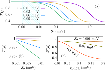
Figure 5: (a) Fidelity of the transfer process as a function of the effective noise intensity $\mathcal{S}_{0}$ for a state prepared with $\theta_{\mathrm{L}}=\pi/4$ and $\phi_{\mathrm{L}}=-\pi/4$ calculated with the Bloch-Redfield master equation, Eq. 28 using the effective Hamiltonian, Eq. 2 in the RWA approximation. The different curves correspond to $\tau=\tau_{\text{LC}}=\tau_{\text{CR}}=10$ (purple), $30$ (yellow), $60$ (blue), and $90$ (green) $\mu$eV. In (b) we have highlighted the range $\mathcal{S}_{0}=1-10$ $\mu\text{eV}$. (c) Fidelity as a function of $\tau_{\text{LC}}=\tau_{\text{CR}}$ for $\mathcal{S}_{0}=0.1$ (red), $0.01$ (green) and $0.001$ (orange)The parameters are as in Fig. 3 with $T=1$ K and infrared cutoff 1 neV.

Contrary to the sweetspots for $\tau_{110}$ and $\tau_{011}$ in the manipulation process, the sweetspot corresponding to the conditions of Eqs 26 and 27, is induced by the ac-voltage. The sweetspot for $\tau_{110}$ in Eq. 19 appears because the dependence on the energies $\epsilon_{i}$ coming from virtual transitions to the $(\uparrow\downarrow,0,0)$ and $(0,\uparrow\downarrow,0)$ states compensate each other. In the sweetspots of Eqs. 26 and 27, however, it is the dependence on the gate energies coming from different ac-induced sidebands that compensate each other.

Finally, the sweetspot condition for deviations from the dark state condition is $\tau_{110}^{(1)}=0$ and $\tau_{011}^{(1)}=\left.\partial_{\epsilon_{\mathrm{R}}}\tau_{011}\right|_{\xi_{\mathrm{CR}}=0}=0$, yielding the same conditions on the gate energies, Eq. 19, as in the manipulation process.

Since direct coupling is the dominant contribution from charge noise, we discuss it in detail. In Sec. V of the Supplementary Information, we write explicitly the Bloch-Redfield operator $Q_{\text{LR}}^{\text{dir}}$ that results from direct coupling to noise (see Eq. 29). We see that there are two contributions. The first is proportional to $\mathcal{S}\left(\Lambda\right)\sin\Upsilon$ and is the one responsible for relaxation, as can be seen from the expression for the relaxation rate due to direct coupling, Eq. 22. The second contribution is proportional to $\mathcal{S}\left(0\right)\cos\Upsilon$ and is the one responsible for dephasing. Since $\mathcal{S}\left(0\right)\gg\mathcal{S}\left(\Lambda\right)$, this is also the most important of the two. However, it vanishes for $\cos\Upsilon=0$, that is, for for $\Upsilon=(2n+1)\pi/2$, $n\mathcal{2}\mathbb{Z}$. From Eq. 23 we see that this corresponds to $\Delta_{\text{LC}}=\Delta_{\text{CR}}$, which includes both the case in which the gradients are negligible or can be turned off, and the linear configuration discussed in Sec. II.3. Hence, this configuration provides the best protection against charge noise.

In Fig. 5 (a) we have plotted the fidelity as a function of $\mathcal{S}_{0}$. We perform the calculations for the case $\Delta_{\text{LC}}=\Delta_{\text{CR}}$ under the dark state condition. We employ values of $\tau_{\text{LR,1}}$ compatible with the values for the exchange interaction in Ref. Dial et al. (2013), corresponding to $\tau_{\text{LC}}=\tau_{\text{CR}}=10$ (purple), $30$ (yellow), $60$ (blue), and $90$ (green) $\mu$eV. In Fig. 5 (b) we have plotted the fidelity in the realistic range $\mathcal{S}_{0}\sim 1-10\mu\text{eV}$Dial et al. (2013); Wu et al. (2014); Qi et al. (2017). For $\tau_{\text{LC}}=\tau_{\text{CR}}=10\,\mu\text{eV}$ we obtain a fidelity of 99.99% for $\mathcal{S}_{0}=1\mu eV$ and of 99.93% for $\mathcal{S}_{0}=10\mu eV$ . Fig. 5 (c) we have plotted the fidelity as a function of $\tau_{\text{LC}}=\tau_{\text{CR}}$ for the different noise intensities $\mathcal{S}_{0}=0.1$ (red), $0.01$ (green) and $0.001$ (orange). By our results we observe that in this realistic range, decreasing $\tau_{\text{LC}},\tau_{\text{CR}}$ increases the total fidelity when considering only charge noise. This can be explained in the following way. For $\Delta_{\text{LC}}=\Delta_{\text{CR}}$, the dominating dephasing process comes from the energy-dependence of the long-range amplitude $\tau_{\mathrm{LR,1}}$. In that case, increasing $\tau_{\text{LC}}$ and $\tau_{\text{CR}}$ to reduce the transfer time also increases the dominant dephasing rate. On the other hand, decreasing $\tau_{\text{LC}},\tau_{\text{CR}}$ reduces $\Lambda$, and in turn increases $\mathcal{S}\left(\Lambda\right)$, but this effect is of lesser importance.

II.4.2 Other sources

Although charge noise is the most significant source of decoherence, magnetic noise caused by the hyperfine coupling and fluctuations in the gradients also detracts from the fidelity. As a result, the spin nuclear bath induces a time-scale, $\mathcal{T}_{2}^{\left(\text{HF}\right)}$, under which the state transfer can be realized with minimal fidelity losses. As shown in Fig. 5 (c), reducing $\tau_{\text{LC}},\tau_{\text{CR}}$ is beneficial to limit the effect of charge noise. If as a result of reducing $\tau_{\text{LC}},\tau_{\text{CR}}$, the transfer time $\mathcal{T}_{\text{LR},1}$ is increased above $\mathcal{T}_{2}^{\left(\text{HF}\right)}$, the hyperfine-induced dephasing disrupts the transferred state. Furthermore, relaxation leads to leakage to the states $\left\{\ket{\uparrow,\uparrow,0},\ket{\downarrow,\downarrow,0},\ket{0,\uparrow,\uparrow},\ket{0,\downarrow,\downarrow}\right\}$, which affects the entanglement $\mathcal{E}(\rho)$ through the concurrence $\mathcal{C}$Note (1). The effect of the hyperfine interaction can be overcome by employing isotope purification in Silicon qubits.

Other effects that may detract from the fidelity are finite ramping timesLi et al. (2017), tunnel noiseRuss et al. (2016); Bello et al. (2017), spin-dependent tunneling ratesDanon and Nazarov (2009); Schreiber et al. (2011) and multiple valley states in SiliconYang et al. (2013); Veldhorst et al. (2015), although most can be reduced by other meansLi et al. (2017).

III Discussion

In summary, we propose a fully tunable two-level system in a double quantum dot contained in one edge of a triple quantum dot structure. By means of ac gate voltages a prepared quantum state in one edge can be transferred to another two-level system defined at the other edge of the TQD by means of photoassisted virtual transitions. The ac voltages fix the prepared state by blocking virtual transitions that modify the desired state and suppress undesired transfer channels via the formation of dark states. In order to measure the information transfer between the two two-level systems we have calculated the time evolution of the states occupations, the phase and their entanglement. The set-up is limited by charge and magnetic noise; the former is induced by random variations in the gate energies and the second by the hyperfine interaction and fluctuations in the gradients. The effect of charge noise can be alleviated by working at the noise sweetspots, where the system is first-order insensitive to charge noise. In that regard, we have shown how the interference between sidebands can induce a sweetspot that does not exist without ac voltages. The latter essentially imposes a time-scale under which the operation can be realized effectively. We show that the protocol has a fidelity $>99\%$ for realistic values of the charge noise intensity and the tunnel barriers.The efficiency of the protocol for quantum state transfer could be improved by considering Si quantum dots where spin flip induced by hyperfine interaction can be strongly reduced through isotope purification. If the transfer times are faster than the decoherence times, the procedure can be generalized to longer quantum dot arrays by using the general state transfer protocol for arbitrary gradient configurations sequentially. Furthermore, the protocol can be implemented experimentally with available technologies, which are no different than those employed to manipulate the exchange interaction in quantum dot-based qubits. Operating in the sweetspots reduces considerably the difficulty in finding the dark state condition required to suppress unwanted processes, leaving the possibility within experimental bounds. We also expect that the technique of dark state formation with ac driving can be employed in the future in other setups to suppress or mitigate processes detrimental to the fidelity of quantum gates or for the possibility of inducing dynamical sweetspots.

Methods

The time-evolution of the density matrix under the assumptions of weak coupling and Markovianity is given by the Bloch-Redfield master equation

$$\dot{\rho}(t) =-i\hbar^{-1}\left[H_{\mathrm{S}},\rho(t)\right]$$

$$-\sum_{i}\left[X_{i},\left[Q_{i},\rho(t)\right]\right]-\sum_{i}\left[X_{i},\left\{R_{i},\rho(t)\right\}\right]$$ (28)

where $\left\{\,,\,\right\}$ indicates the anti-commutator and

$$Q_{i}=\frac{1}{\pi}\int_{0}^{\infty}d\tau\int_{0}^{\infty}d\omega\mathcal{S}(\omega)\tilde{X}_{i}(\tau,0)\cos(\omega\tau)$$ (29)

$$R_{i}=\frac{1}{i\pi}\int_{0}^{\infty}d\tau\int_{0}^{\infty}d\omega\mathcal{J}(\omega)\tilde{X}_{i}(\tau,0)\sin(\omega\tau)$$ (30)

We define the propagated system operators as $\tilde{X}_{i}(\tau,\tau^{\prime})=\mathcal{U}^{\dagger}(\tau,\tau^{\prime})X_{i}\mathcal{U}(\tau,\tau^{\prime})$. Apart from $X_{i}=\hat{c}_{i}^{\dagger}\hat{c}_{i}$, we have to consider the coupling between system and bath through the virtual tunneling processes, which depend on the energy differences between the states.

For sections II.2 and II.3, results are obtained without any source of decoherence. Then, Eq. 28 reduces to $\dot{\rho}(t)=-i\hbar^{-1}\left[H_{\mathrm{S}},\rho(t)\right]$. In these sections, the results are obtained with $H_{\text{S}}$ corresponding to the full Hamiltonian of Eq. 1. For section II.4, the calculations are performed with the master equation, Eq. 28. The Hamiltonian $H_{\text{\text{$S$}}}$ for this section is the effective Hamiltonian of Eq. 2 in the time-independent RWA. The incoherent terms appearing in Eq. 28 are discussed the Supplementary Information.

Contributions

J. Picó-Cortés and F. Gallego-Marcos have contributed in developing the theoretical model and the numerical calculations. G. Platero has contributed in developing the theoretical model and has supervised the work.