Quantum steering is a kind of quantum correlations stronger than entanglement but weaker than Bell-nonlocality. In an optomechanical system pumped by squeezed light and driven in the red sideband, we study-under thermal effects-stationary Gaussian steering and its asymmetry of two mechanical modes. In the resolved sideband regime using experimentally feasible parameters, we show that Gaussian steering can be created by quantum fluctuations transfer from the squeezed light to the two mechanical modes. Moreover, one-way steering can be observed by controlling the squeezing degree or the environmental temperature. A comparative study between Gaussian steering and Gaussian Rényi-2 entanglement of the two considered modes shows on one hand that both steering and entanglement suffer from a sudden death-like phenomenon with early vanishing of steering in various circumstances. On the other hand, steering is found stronger than entanglement, however, remains constantly upper bounded by Gaussian Rényi-2 entanglement, and decays rapidly to zero under thermal noise.

1 Introduction

In their seminal 1935 paper [1], Einstein, Podolsky, and Rosen (EPR) have highlighted that, when two spatially separated particles are entangled, two arbitrary local measurements performed upon one particle induce immediate nonlocal effects on the second, where this end may be left in states with two different wave-functions. To capture the essence of this spooky action-at-a-distance phenomenon on one hand, and to generalize the EPR paradox on the other hand, Schrödinger has originally introduced the concept of steer as an exotic quantum effect allowing remotely preparation of quantum states by local operations [2]. Recently, quantum steering or EPR steering was defined as a kind of non-separable quantum correlations [3], weaker than Bell nonlocality [4], but stronger than entanglement [5]. Precisely, for a given quantum bipartite state, the violation of Bell inequality implies EPR steering in both directions, while, steering at least in one direction implies that the state is entangled [3]. Interestingly enough, moving from entanglement to EPR steering to Bell-nonlocality; requires decreasing the number of observers and apparatuses that must be trusted [3]. In contrast, the corresponding protocols were shown to be progressively less robust against thermal noise for projective measurements [6].

From an operational perspective in quantum information theory, EPR steering corresponds to an entanglement verification task, i.e. it certifies the existence of entanglement between two parties, assuming trusted measurements only on one side. Specifically, if Alice and Bob jointly share a steerable state at least in one direction (say from Alice to Bob), then, Alice can convince Bob who does not trust her that their shared state is entangled, by performing local operations and classical communication.

On the basis of the uncertainty principle, a quantitative criterion to test the experimental EPR paradox was proposed in [7]. Further, it has been proven that the violation of such criterion under Gaussian measurements witnesses EPR steering [3], where the first verification was realised in [8].

To detect quantum steering, several inequalities are available [9], where their violation certifies EPR steering [10], however, they cannot quantify it [11]. In this sense, two steering quantifiers were proposed, i.e. steering weight [12], and the steering robustness [13]. Unfortunately, both quantifiers are not evaluated in a compact form, where they can only be computed numerically by semidefinite programming [11], while, for two-mode Gaussian states, a computable measure was developed [14].

Actually, our knowledge concerning the generation, the detection and also the quantification of EPR steering has significantly advanced, where intense efforts have been made in the last decade to study such phenomenon theoretically [15, 16] as well as experimentally [17, 18, 19].

Importantly, the distinctive feature of EPR steering-unlike entanglement and Bell nonlocality-that is intrinsically asymmetric, i.e. an entangled quantum state may be steerable from Alice to Bob, but not vice versa, which is commonly known as one-way steering [3, 14]. Apart from its fundamental relevance, one-way steering has attracted a great deal of attention [19, 20, 21], where it has been appreciated as a resource for various quantum information protocols, e.g. one-sided device-independent quantum cryptography [22], secure quantum teleportation [23], and subchannel discrimination [13].

Restricting to Gaussian states and measurements, experimental one-way steering was carried out in [24] and later in [25], which answer genuinely the question already raised by Wiseman et al, i.e. are there entangled states which are one-way steerable [3]. We recall that pure entangled states cannot exhibit one-way steering, where they can always be transformed to a symmetric form via local basis change using the Schmidt decomposition [19].

We note here that in an optical setup, one-way steering has been proven theoretically and then experimentally observed under Gaussian and non-Gaussian measurements in Ref. [21]. While, in hybrid optomechanical systems, such behavior has been studied considering Gaussian measurements on Gaussian states in Refs. [26, 27]. In this paper, using two spatially separated optomechanical cavities coupled to two-mode squeezed light and driven in the red sideband, we investigate-under thermal effects-Gaussian EPR steering of two non-interacting mechanical modes, where a particular attention is dedicated to the one-way steering behavior. Also, we compare the Gaussian steering of the two considered modes with their Gaussian Rényi-2 entanglement [28].

Over the past decades, substantial efforts in optomechanics have been made to test quantum effects [29, 30]. This includes, cooling of a mechanical oscillator to its ground state [31], optomechanically induced transparency [32], quantum squeezing [33], macroscopic superposition state [34], backaction-evading measurement [35], quantum entanglement [36] and also quantum steering [26, 27].

This paper is organized as follows. In Sec. 2, we introduce the basic optomechanical system involving two optical modes and two mechanical modes. Next, using the dynamics based on the quantum Langevin equations, we derive in the resolved sideband regime the covariance matrix describing stationary four-mode Gaussian states of the system. In Sec. 3, focusing on the mechanical modes, we quantify their Gaussian steering as well as their Gaussian Rényi-2 entanglement. We study and compare these two different aspects of non-separable quantum correlations under thermal noises induced by the squeezing effect and the environmental temperatures. In Sec. 4, we draw our conclusions.

2 A Fabry-Pérot double-cavity optomechanical system

2.1 Model and Hamiltonian

Figure 1: A double-cavity optomechanical system driven in the red sideband and fed by two-mode squeezed light with input noise operators $\mathfrak{F}_{1,2}^{in}$. Each movable mirror oscillates at frequency $\omega_{m_{j}}$.

The proposed optomechanical system comprises two Fabry-Pérot cavities (Fig. 1), where each cavity is composed by two mirrors. The first one is fixed and partially transmitting, while, the second is movable and perfectly reflecting. The $j\mathrm{th}$ cavity has length $l_{j}$ and driven by coherent laser with input power ${\wp}_{j}$, phase $\varphi_{j}$ and frequency $\omega_{L_{j}}$. Also, the two cavities are fed by two-mode squeezed light of frequency $\omega_{s}$. The first(second) squeezed mode is sent towards the first(second) cavity.
The two Fabry-Pérot cavities can be described by the following Hamiltonian ($\hbar=1$) [37]

$$\mathcal{\hat{H}=}\sum_{j=1}^{2}\Big{(}\mathcal{\hat{H}}_{c_{j}}\mathcal{+\hat{H}}_{m_{j}}\mathcal{+\hat{H}}_{coup_{j}}\mathcal{+\hat{H}}_{drive_{j}}\Big{)},$$ (1)

where $\mathcal{\hat{H}}_{c_{j}}=\omega_{c_{j}}a_{j}^{{\dagger}}a_{j}$ is the free Hamiltonian of the $j\mathrm{th}$ cavity mode with annihilation operator $a_{j}$, frequency $\omega_{c_{j}}$ and decay rate $\kappa_{c_{j}}$, while, $\mathcal{\hat{H}}_{m_{j}}=\omega_{m_{j}}b_{j}^{{\dagger}}b_{j}$ is the free Hamiltonian of the $j\mathrm{th}$ movable mirror modeled as a single-mode quantum harmonic oscillator with annihilation operator $b_{j}$, an effective mass $\mu_{j}$, frequency $\omega_{m_{j}}$ and damping rate $\gamma_{m_{j}}$. The term $\mathcal{\hat{H}}_{coup_{j}}=\chi_{0_{j}}a_{j}^{{\dagger}}a_{j}(b_{j}^{{\dagger}}+b_{j})$ is the radiation pressure coupling between the $j\mathrm{th}$ cavity mode and its corresponding mechanical mode, with coupling rate $\chi_{0_{j}}=\left(\omega_{c_{j}}/l_{j}\right)\sqrt{\hbar/\mu_{{}_{j}}\omega_{m_{j}}}$. Finally, $\mathcal{\hat{H}}_{drive_{j}}=\varepsilon_{j}(a_{j}^{{\dagger}}e^{i\varphi_{j}}e^{-i\omega_{L_{j}}}+a_{j}e^{-i\varphi_{j}}e^{i\omega_{L_{j}}})$ is the coupling between the $j\mathrm{th}$ laser and the $j\mathrm{th}$ cavity, with coupling strength $\varepsilon_{j}=\sqrt{2\kappa_{c_{j}}{\wp}_{j}/\hbar\omega_{L_{j}}}$.

2.2 System dynamics

The system at hand is a dissipative-noisy optomechanical system. So, the dynamics can be conveniently described by the quantum Langevin equation,i.e.$\partial_{t}\mathcal{O}=\frac{1}{i\hbar}\left[\mathcal{O},\mathcal{\hat{H}}\right]+dissipation$ $and$ $noise$ $terms$ ($\mathcal{O\equiv}a_{j},b_{j}$) [38]. Thus, in a frame rotating with $\omega_{L_{j}}$, we obtain the following nonlinear equations

$$\partial_{t}b_{j} = -\left(\frac{\gamma_{m_{j}}}{2}+i\omega_{m_{j}}\right)b_{j}-i\chi_{0_{j}}a_{j}^{{\dagger}}a_{j}+\sqrt{\gamma_{m_{j}}}\zeta_{j}^{in},$$ (2)

$$\partial_{t}a_{j} = -\left(\frac{\kappa_{c_{j}}}{2}-i\Delta_{j}\right)a_{j}-i\chi_{0_{j}}a_{j}(b_{j}^{{\dagger}}+b_{j})-i\varepsilon_{j}e^{i\varphi_{j}}+\sqrt{\kappa_{c_{j}}}\mathfrak{F}_{j}^{in},$$ (3)

with $\Delta_{j}=\omega_{L_{j}}-\omega_{c_{j}}$ is the $j\mathrm{th}$ laser detuning [30]. $\zeta_{j}^{in}$ is the zero-mean Brownian noise operator affecting the $j\mathrm{th}$ movable mirror. It is not in general $\delta$-correlated, exhibiting a non-Markovian correlation function between two instants $t$ and $t^{\prime}$ [39]. However, oscillators with large mechanical quality factor $\mathcal{Q}_{m_{j}}=\omega_{m_{j}}/\gamma_{m_{j}}\gg 1$ allows recovering the Markovian process and, then, quantum effects can be reached. In this limit, we have the following nonzero time-domain correlation functions [40]

$$\langle\zeta_{j}^{in{\dagger}}(t)\zeta_{j}^{in}(t^{\prime});\zeta_{j}^{in}(t)\zeta_{j}^{in{\dagger}}(t^{\prime})\rangle=\Big{(}n_{th,j};n_{th,j}+1\Big{)}\delta(t-t^{\prime}),\text{ \ }j=1,2,$$ (4)

with $n_{th,j}=(e^{\hbar\omega_{m_{j}}/k_{B}T_{j}}-1)^{-1}$ is the $j\mathrm{th}$ mean number of phonons. $T_{j}$ and $k_{B}$ are the temperature of the $j\mathrm{th}$ mirror environment and the Boltzmann constant. In Eq. (3), $\mathfrak{F}_{j}^{in}$ is the $j\mathrm{th}$ zero mean input squeezed noise operator, with the following nonzero time-domain correlation functions [38]

$$\langle\delta\mathfrak{F}_{j}^{in^{{\dagger}}}(t)\delta\mathfrak{F}_{j}^{in}(t^{\prime});\delta\mathfrak{F}_{j}^{in}(t)\delta\mathfrak{F}_{j}^{in^{{\dagger}}}(t^{\prime})\rangle = \Big{(}N;N+1\Big{)}\delta(t-t^{\prime}),\text{ \ }j=1,2,$$ (5)

$$\langle\delta\mathfrak{F}_{j}^{in}(t)\delta\mathfrak{F}_{j^{\prime}}^{in}(t^{\prime});\delta\mathfrak{F}_{j}^{in^{{\dagger}}}(t)\delta\mathfrak{F}_{j^{\prime}}^{in^{{\dagger}}}(t^{\prime})\rangle = \Big{(}Me^{-i\omega_{m}\left(t+t^{\prime}\right)};Me^{i\omega_{m}\left(t+t^{\prime}\right)}\Big{)}\delta(t-t^{\prime}),\text{ \ }j\neq j^{\prime}=1,2,$$ (6)

with $N=\mathrm{sinh}^{\mathrm{2}}r$, $M=\mathrm{sinh}r\mathrm{cosh}r$, $r$ is the squeezing parameter (we have assumed that $\omega_{m_{1,2}}=\omega_{m}$). We note that optimal transfer from the squeezed light to the mechanical degrees of freedom can be achieved when the frequency of the squeezing is resonant with those of the cavities,i.e. $\omega_{s}=\omega_{c_{j}}$ [41].

2.3 Linearization of the dynamics around the steady-states

The equations (2)-(3) are nonlinear due to the quadratic terms $a_{j}^{{\dagger}}a_{j}$, $a_{j}b_{j}^{{\dagger}}$ and $a_{j}b_{j}$, then, they cannot be solved exactly [39]. Assuming weak coupling between the $j\mathrm{th}$ cavity mode and its associated mechanical mode, the fluctuations $\delta a_{j}$, $\delta b_{j}$ are much smaller than the steady-state mean values $\langle a_{j}\rangle$ and $\langle b_{j}\rangle$. So, we can linearize the dynamics around the steady state, where each operator can be written as sum of its steady-state mean value and a small fluctuation with zero mean value,i.e. $\mathcal{O}_{j}=\langle\mathcal{O}_{j}\rangle+\delta\mathcal{O}_{j}$ ($\mathcal{O}_{j}\equiv a_{j},b_{j}$) [39]. The mean values are obtained by setting the time derivatives to zero and factorizing the averages in Eqs. (2)-(3). Thus, we get $\langle a_{j}\rangle\equiv a_{js}=\frac{-2i\varepsilon_{j}e^{i\varphi_{j}}}{\kappa_{c_{j}}-2i\Delta_{j}^{\prime}}$ and $\langle b_{j}\rangle\equiv b_{js}=\frac{-2i\chi_{0_{j}}\left|a_{js}\right|^{2}}{\gamma_{m_{j}}+2i\omega_{m_{j}}}$ with $\Delta_{j}^{\prime}$ $=$ $\Delta_{j}$ $-\chi_{0_{j}}(b_{js}{}^{\ast}+b_{js})$ is the $j\mathrm{th}$ effective detuning [30]. To simplify further our purpose, we assume that the two cavities are intensely driven,i.e. $\left|a_{js}\right|\gg 1$ by lasers with large powers $\wp_{1,2}$ [39]. So, the terms $\delta a_{j}^{{\dagger}}\delta a_{j}$, $\delta a_{j}\delta b_{j}$ and $\delta a_{j}\delta b_{j}^{{\dagger}}$ can be safely neglected, leading to

$$\delta\dot{b}_{j} = -\left(\frac{\gamma_{m_{j}}}{2}+i\omega_{m_{j}}\right)\delta b_{j}+\chi_{j}\left(\delta a_{j}-\delta a_{j}^{{\dagger}}\right)+\sqrt{\gamma_{m_{j}}}\zeta_{j}^{in},$$ (7)

$$\delta\dot{a}_{j} = -\left(\frac{\kappa_{c_{j}}}{2}-i\Delta_{j}^{\prime}\right)\delta a_{j}-\chi_{j}\left(\delta b_{j}+\delta b_{j}^{{\dagger}}\right)+\sqrt{\kappa_{c_{j}}}\delta\mathfrak{F}_{j}^{in},$$ (8)

$\chi_{j}$ $=\chi_{0_{j}}\left|a_{js}\right|$ being the $j\mathrm{th}$ effective coupling [30]. Notice that Eqs. (7)-(8) are obtained by setting $a_{js}=-i\left|a_{js}\right|$ or equivalently to $\tan\varphi_{j}=-2\Delta_{j}^{\prime}/\kappa_{c_{j}}$. Next, we introduce the operators $\delta\tilde{b}_{j}=\delta b_{j}e^{i\omega_{m_{j}}t}$ and $\delta\tilde{a}_{j}=\delta a_{j}e^{-i\Delta_{j}^{\prime}t}$ and we assume that the system is driven in the red sideband ($\Delta_{j}^{\prime}=-\omega_{m_{j}}$), which is appropriate for quantum-state transfer [30]. Moreover, in the resolved-sideband regime,i.e. $\omega_{m_{j}}\gg\kappa_{c_{j}}$, the rotating wave approximation (RWA) allows to drop terms rotating at $\pm 2\omega_{m_{j}}$ [42]. Thus, one has

$$\delta\dot{\tilde{b}}_{j} = -\frac{\gamma_{m_{j}}}{2}\delta\tilde{b}_{j}+\chi_{j}\delta\tilde{a}_{j}+\sqrt{\gamma_{m_{j}}}\tilde{\zeta}_{j}^{in},$$ (9)

$$\delta\dot{\tilde{a}}_{j} = -\frac{\kappa_{c_{j}}}{2}\delta\tilde{a}_{j}-\chi_{j}\delta\tilde{b}_{j}+\sqrt{\kappa_{c_{j}}}\delta\mathfrak{\tilde{F}}_{j}^{in}.$$ (10)

2.4 Four-mode covariance matrix

Using Eqs. (9)-(10) and the quadratures position and momentum of the $j\mathrm{th}$ mechanical(optical) mode $\delta\tilde{q}_{m_{j}}=(\delta\tilde{b}_{j}^{{\dagger}}+\delta\tilde{b}_{j})/\sqrt{2}$ and $\delta\tilde{p}_{m_{j}}=i(\delta\tilde{b}_{j}^{{\dagger}}-\delta\tilde{b}_{j})/\sqrt{2}$ $\Big{(}\delta\tilde{q}_{c_{j}}=(\delta\tilde{a}_{j}^{{\dagger}}+\delta\tilde{a}_{j})/\sqrt{2}$ and $\delta\tilde{p}_{c_{j}}=i(\delta\tilde{a}_{j}^{{\dagger}}-\delta\tilde{a}_{j})/\sqrt{2}\Big{)}$ with their corresponding input mechanical(optical) noise operators $\delta\tilde{q}_{m_{j}}^{in}=(\tilde{\zeta}_{j}^{in\dagger}+\tilde{\zeta}_{j}^{in})/\sqrt{2}$ and $\delta\tilde{p}_{m_{j}}^{in}=i(\tilde{\zeta}_{j}^{in\dagger}-\tilde{\zeta}_{j}^{in})/\sqrt{2}$ $\Big{(}\delta\tilde{q}_{c_{j}}^{in}=(\delta\mathfrak{\tilde{F}}_{j}^{in{\dagger}}+\delta\mathfrak{\tilde{F}}_{j}^{in})/\sqrt{2}$ and $\delta\tilde{p}_{c_{j}}^{in}=i(\delta\mathfrak{\tilde{F}}_{j}^{in{\dagger}}-\delta\mathfrak{\tilde{F}}_{j}^{in})/\sqrt{2}\Big{)}$, we obtain

$$\partial_{t}\delta\tilde{q}_{m_{j}} = -\frac{\gamma_{m_{j}}}{2}\delta\tilde{q}_{m_{j}}+\chi_{j}\delta\tilde{q}_{c_{j}}+\sqrt{\gamma_{m_{j}}}\delta\tilde{q}_{m_{j}}^{in},$$ (11)

$$\partial_{t}\delta\tilde{p}_{m_{j}} = -\frac{\gamma_{m_{j}}}{2}\delta\tilde{p}_{m_{j}}+\chi_{j}\delta\tilde{p}_{c_{j}}+\sqrt{\gamma_{m_{j}}}\delta\tilde{p}_{m_{j}}^{in},$$ (12)

$$\partial_{t}\delta\tilde{q}_{c_{j}} = -\frac{\kappa_{c_{j}}}{2}\delta\tilde{q}_{c_{j}}-\chi_{j}\delta\tilde{q}_{m_{j}}+\sqrt{\kappa_{c_{j}}}\delta\tilde{q}_{c_{j}}^{in},$$ (13)

$$\partial_{t}\delta\tilde{p}_{c_{j}} = -\frac{\kappa_{c_{j}}}{2}\delta\tilde{p}_{c_{j}}-\chi_{j}\delta\tilde{p}_{m_{j}}+\sqrt{\kappa_{c_{j}}}\delta\tilde{p}_{c_{j}}^{in},$$ (14)

which can be written as $\partial_{t}\tilde{u}=\mathcal{A}\tilde{u}+\tilde{n}$, with $\tilde{u}^{\mathrm{T}}=(\delta\tilde{q}_{m_{1}},\delta\tilde{p}_{m_{1}},\delta\tilde{q}_{m_{2}},\delta\tilde{p}_{m_{2}},\delta\tilde{q}_{c_{1}},\delta\tilde{p}_{c_{1}},\delta\tilde{q}_{c_{2}},\delta\tilde{p}_{c_{2}})$, $\tilde{n}^{\mathrm{T}}=(\delta\tilde{q}_{m_{1}}^{in},\delta\tilde{p}_{m_{1}}^{in},\delta\tilde{q}_{m_{2}}^{in},\delta\tilde{p}_{m_{2}}^{in},\delta\tilde{q}_{c_{1}}^{in},\delta\tilde{p}_{c_{1}}^{in},\delta\tilde{q}_{c_{2}}^{in},\delta\tilde{p}_{c_{2}}^{in})$ and $\mathcal{A=}\left(\begin{array}[]{cc}\mathcal{A}_{\gamma_{m}}&\mathcal{A}_{\chi_{+}}\\ \mathcal{A}_{\chi_{-}}&\mathcal{A}_{\kappa_{c}}\end{array}\right)$, wherein the $2\times 2$ blocks matrices $\mathcal{A}_{\gamma_{m}}$, $\mathcal{A}_{\kappa_{c}}$ and $\mathcal{A}_{\chi_{\pm}}$ are respectively given by $\mathcal{A}_{\gamma_{m}}=\mathrm{diag}(-\frac{\gamma_{m_{1}}}{2},-\frac{\gamma_{m_{1}}}{2},-\frac{\gamma_{m_{2}}}{2},-\frac{\gamma_{m_{2}}}{2})$, $\mathcal{A}_{\kappa_{c}}=\mathrm{diag}(-\frac{\kappa_{c_{1}}}{2},-\frac{\kappa_{c_{1}}}{2},-\frac{\kappa_{c_{2}}}{2},-\frac{\kappa_{c_{2}}}{2})$ and $\mathcal{A}_{\chi_{\pm}}=\mathrm{diag}(\pm\chi_{1},\pm\chi_{1},\pm\chi_{2},\pm\chi_{2})$.
Since the dynamics is linearized and $\zeta_{j}^{in}$ and $\mathfrak{F}_{j}^{in}$ are zero-mean quantum Gaussian noises, the steady-state of the quantum fluctuations is a zero-mean quadripartite Gaussian state and then, it can be described by its $8\times 8$ covariance matrix $\mathcal{V}$ defined as $\mathcal{V}_{kk^{\prime}}=\left(\langle\tilde{u}_{k}(\infty)\tilde{u}_{k^{\prime}}(\infty)+\tilde{u}_{k^{\prime}}(\infty)\tilde{u}_{k}(\infty)\rangle\right)/2$ [39].
Using standard approaches [39, 43], one can determine the matrix $\mathcal{V}$ by solving the Lyapunov equation

$$\mathcal{AV+VA}^{\mathrm{T}}=-\mathcal{D},$$ (15)

where $\mathcal{D}$ the diffusion matrix defined by $\mathcal{D}_{jj^{\prime}}\delta(t-t^{\prime})=\left(\langle\tilde{n}_{j}(t)\tilde{n}_{j^{\prime}}(t^{\prime})+\tilde{n}_{j^{\prime}}(t^{\prime})\tilde{n}_{j}(t)\rangle\right)/2$ can be written as $\mathcal{D=D}_{\gamma_{m}}\oplus\mathcal{D}_{\kappa_{c}}$ with $\mathcal{D}_{\gamma_{m}}=\mathrm{diag}\Big{(}\gamma_{m_{1}}(n_{th,1}+\frac{1}{2}),\gamma_{m_{1}}(n_{th,1}+\frac{1}{2}),\gamma_{m_{2}}(n_{th,2}+\frac{1}{2}),\gamma_{m_{2}}(n_{th,2}+\frac{1}{2})\Big{)}$ and

$$\mathcal{D}_{\kappa_{c}}=\left(\begin{array}[]{cccc}\frac{\kappa_{c_{1}}}{2}\cosh(2r)&0&\frac{\sqrt{\kappa_{c_{1}}\kappa_{c_{2}}}}{2}\sinh(2r)&0\\ 0&\frac{\kappa_{c_{1}}}{2}\cosh(2r)&0&\frac{-\sqrt{\kappa_{c_{1}}\kappa_{c_{2}}}}{2}\sinh(2r)\\ \frac{\sqrt{\kappa_{c_{1}}\kappa_{c_{2}}}}{2}\sinh(2r)&0&\frac{\kappa_{c_{2}}}{2}\cosh(2r)&0\\ 0&\frac{-\sqrt{\kappa_{c_{1}}\kappa_{c_{2}}}}{2}\sinh(2r)&0&\frac{\kappa_{c_{2}}}{2}\cosh(2r)\end{array}\right).$$ (16)

The covariance matrix (CM) $\mathcal{V}$ solution of Eq. (15), can be expressed as

$$\mathcal{V=}\left[\mathcal{V}_{ij}\right]_{8\times 8}\mathcal{=}\left(\begin{array}[]{cccc}\mathcal{V}_{m_{1}}&\mathcal{V}_{m_{12}}&\mathcal{V}_{m_{1}c_{1}}&\mathcal{V}_{m_{1}c_{2}}\\ \mathcal{V}_{m_{12}}^{\mathrm{T}}&\mathcal{V}_{m_{2}}&\mathcal{V}_{m_{2}c_{1}}&\mathcal{V}_{m_{2}c_{2}}\\ \mathcal{V}_{m_{1}c_{1}}^{\mathrm{T}}&\mathcal{V}_{m_{2}c_{1}}^{\mathrm{T}}&\mathcal{V}_{c_{1}}&\mathcal{V}_{c_{12}}\\ \mathcal{V}_{m_{1}c_{2}}^{\mathrm{T}}&\mathcal{V}_{m_{2}c_{2}}^{\mathrm{T}}&\mathcal{V}_{c_{12}}^{\mathrm{T}}&\mathcal{V}_{c_{2}}\end{array}\right),$$ (17)

where the $2\times 2$ blocks matrices $\mathcal{V}_{m_{1}}$ and $\mathcal{V}_{m_{2}}$ ($\mathcal{V}_{c_{1}}$ and $\mathcal{V}_{c_{2}}$) represent the first and second mechanical(optical) modes, while their correlations are described by $\mathcal{V}_{m_{12}}$($\mathcal{V}_{c_{12}}$). Moreover, the matrix $\mathcal{V}_{m_{i}c_{j}}$ ($i,j\in\{1,2\}$) describes the correlations between the $i\mathrm{th}$ mechanical mode and the $j\mathrm{th}$ optical mode.
Since we are interested in the Gaussian steering of the two mechanical modes labeled as $A$ and $B$, their covariance matrix $\mathcal{V}_{m}$ can be obtained by tracing over the uninteresting block matrices in (17). Thus, one has

$$\mathcal{V}_{m}=\left(\begin{array}[]{cc}\mathcal{V}_{m_{1}}&\mathcal{V}_{m_{12}}\\ \mathcal{V}_{m_{12}}^{\mathrm{T}}&\mathcal{V}_{m_{2}}\end{array}\right),$$ (18)

with $\mathcal{V}_{m_{1}}=\mathrm{diag}(\upsilon_{1},\upsilon_{1})$, $\mathcal{V}_{m_{2}}=\mathrm{diag}(\upsilon_{2},\upsilon_{2})$ and $\mathcal{V}_{m_{12}}=\mathrm{diag}(\upsilon_{12},-\upsilon_{12})$.
Assuming identical dampings,i.e.$\gamma_{m_{1,2}}=\gamma_{m}$ and $\kappa_{c_{1,2}}=\kappa_{c}$, the matrix elements $\upsilon_{1}$, $\upsilon_{2}$ and $\upsilon_{12}$ are

$$\upsilon_{j} = \frac{\left(1+2n_{th,j}\right)\left(1+\tau+\tau\mathcal{C}_{j}\right)+\mathcal{C}_{j}\cosh(2r)}{2\left(1+\tau\right)\left(1+\mathcal{C}_{j}\right)},\text{ for \ }j=1,2,$$ (19)

$$\upsilon_{12} = \frac{\sqrt{\mathcal{C}_{1}\mathcal{C}_{2}}\left(1+\tau\right)\sinh(2r)}{\left(2+\mathcal{C}_{1}+\mathcal{C}_{2}\right)\left(1+\tau\right)^{2}+\frac{\tau}{2}\left(\mathcal{C}_{1}-\mathcal{C}_{2}\right)^{2}},$$ (20)

where $\tau=\gamma_{m}/\kappa_{c}$ is the damping ratio and $\mathcal{C}_{j}$ is the $j\mathrm{th}$ optomechanical cooperativity defined by [44]

$$\mathcal{C}_{j}=4\chi_{j}^{2}/\gamma_{m}\kappa_{c}=\frac{8\omega_{c_{j}}^{2}\wp_{j}}{\gamma_{m}\mu_{{}_{j}}\omega_{m_{j}}\omega_{L_{j}}l_{j}^{2}\left[\left(\frac{\kappa_{c}}{2}\right)^{2}+\omega_{{}_{m_{j}}}^{2}\right]},$$ (21)

Based on Eqs. (18)-(20), we remark that if at least one of the three parameters $\mathcal{C}_{1}$, $\mathcal{C}_{2}$ or $r$ is zero, then $\upsilon_{12}=0$, $\det\mathcal{V}_{m_{12}}$ will be as well. This implies that the CM $\mathcal{V}_{m}$ (18) describing the two mechanical modes $A$ and $B$ is a Gaussian product states [45]. So, the two modes $A$ and $B$ remain unentangled and, therefore, they can not be steerable neither from $A\rightarrow B$ nor from $B\rightarrow A$ [14]. This is because $\det\mathcal{V}_{m_{12}}$ $<0$ is a necessary condition for a two-mode Gaussian states $\varrho_{AB}$ to be entangled [46]. Finally, it should be aware that the stability conditions have been verified, where they are always satisfied in the chosen parameter regime. This can be explained by the fact that the two cavities are driven in the red sideband [39].

3 Gaussian EPR steering vs Gaussian Rényi-2 entanglement

3.1 Gaussian EPR steering

To study the Gaussian EPR steering of the two mechanical modes $A$ and $B$, we adopt the measure proposed in [14]. For arbitrary two-mode Gaussian states with covariance matrix $\mathcal{V}_{m}$ (18), Alice can steer the Bob’s states by performing Gaussian measurements, if the following condition is violated [3]

$$\mathcal{V}_{m}+i(0_{A}\oplus\Omega_{B})\geqslant 0,$$ (22)

where $0_{A}$ is a $2\times 2$ null matrix and $\Omega_{B}$ $=\left(\begin{array}[]{cc}0&1\\ -1&0\end{array}\right)$ is the $B$-mode symplectic matrix [14]. Henceforth, the violation of the condition (22) is necessary and sufficient for Gaussian $A\rightarrow B$ steerability [14].
To quantify how much an arbitrary bipartite Gaussian state with CM $\mathcal{V}_{m}$ is steerable under Gaussian measurements on Alice’s side, Kogias et al have been proposed the following measure [14]

$$\mathcal{G}^{A\rightarrow B}(\mathcal{V}_{m}):=\max\{0,-\ln(\eta^{B})\},$$ (23)

where $\eta^{B}=\sqrt{\det(\mathcal{V}_{m_{2}}-\mathcal{V}_{m_{12}}^{\mathrm{T}}\mathcal{V}_{m_{1}}^{-1}\mathcal{V}_{m_{12}})}$.
The steering $\mathcal{G}^{A\rightarrow B}$ is monotone under Gaussian LOCC [47], it quantifies the amount by which the condition (22) fails to be fulfilled and vanishes if the state described by $\mathcal{V}_{m}$ is nonsteerable by Alice’s measurements [14]. For two-mode Gaussian states, Eq. (23) becomes $\mathcal{G}^{A\rightarrow B}=\max\left[0,\frac{1}{2}\ln\frac{\det\mathcal{V}_{m_{1}}}{4\det\mathcal{V}_{m}}\right]$, where $\mathcal{G}^{B\rightarrow A}$ can be obtained by changing the roles of $A$ and $B$ in Eq. (23) [14].
Unlike entanglement and Bell non-locality, EPR steering is an asymmetric aspect of quantum nonlocality,i.e. a quantum state $\varrho_{AB}$ may be steerable from Alice to Bob, but not vice versa [14]. Therefore, we distinguish three cases. The first one corresponding to no-way steering, where the state is nonsteerable in any direction,i.e. $\mathcal{G}^{A\rightarrow B}=\mathcal{G}^{B\rightarrow A}=0$. The second case referring to two-way steering, where the state is steerable in both directions,i.e. $\mathcal{G}^{A\rightarrow B}>0$ and $\mathcal{G}^{B\rightarrow A}>0$. Finally, the third case in which the state is steerable only in one direction,i.e. $\mathcal{G}^{A\rightarrow B}>0$ and $\mathcal{G}^{B\rightarrow A}=0$ or $\mathcal{G}^{A\rightarrow B}=0$ and $\mathcal{G}^{B\rightarrow A}>0$, which corresponds to one-way steering. This last case reflecting the asymmetric nature of quantum correlations is conjectured to play a decisive role in various communication protocols [11].
To check how asymmetric can the steerability be in two-mode Gaussian states $\varrho_{AB}$, we use the steering asymmetry defined as $\mathcal{G}_{AB}^{\Delta}=\left|\mathcal{G}^{A\rightarrow B}-\mathcal{G}^{B\rightarrow A}\right|$ [14]. It has been proven on the one hand that $\mathcal{G}_{AB}^{\Delta}$ can never exceed $\ln 2$; it is maximal when the state is one-way steerable, and it decreases with increasing steerability in either way, on the other hand, the Gaussian steering is always upper bounded by the Gaussian Rényi-2 entanglement $\mathcal{E}_{2}$ with equality on pure states [14].

3.2 Gaussian Rényi-2 entanglement

In quantum information theory, Rényi-$\alpha$ entropies are a family of additive entropies, providing a generalized spectrum of measures of information in a quantum state $\varrho$ [48]. They are defined as $\mathcal{S}_{\alpha}(\varrho)=(1-\alpha)^{-1}\ln\mathrm{Tr}\left(\varrho^{\alpha}\right)$, where in the limit $\alpha\rightarrow 1$, $\mathcal{S}_{\alpha}(\varrho)$ reduces to the von Neumann entropy $\mathcal{S}(\varrho)=-\mathrm{Tr}\left(\varrho\ln\varrho\right)$, while $\mathcal{S}_{2}(\varrho)=-\ln\mathrm{Tr}\left(\varrho^{2}\right)$ corresponds to Rényi-2 entropy [28]. It has been proven that for Gaussian states, Rényi-2 entropy satisfies the strong subadditivity inequality,i.e. $\mathcal{S}_{2}\left(\mathcal{\varrho}_{AB}\right)+\mathcal{S}_{2}\left(\mathcal{\varrho}_{BC}\right)\geqslant\mathcal{S}_{2}\left(\mathcal{\varrho}_{ABC}\right)+\mathcal{S}_{2}\left(\mathcal{\varrho}_{B}\right)$, therefore it can be used to define valid Gaussian measures of information and correlation quantities, encompassing entanglement [28].
For generally mixed two-mode Gaussian states $\mathcal{\varrho}_{AB}$, the Rényi-2 entanglement measure $\mathcal{E}_{2}\mathcal{(\varrho}_{AB}\mathcal{)\equiv E}_{2}$, is not amenable to analytical evaluation and can only be computed numerically by semidefinite programming [28, 46]. However, for some subclasses of bi-mode Gaussian states including symmetric states [49], squeezed thermal states (STS) [45] and GLEMS-Gaussian states of partial minimum uncertainty [46], Gaussian Rényi-2 entanglement (GR2E) can be compactly expressed [46].
The covariance matrix $\mathcal{V}_{m}$ (18) is in the standard form, where $\mathcal{V}_{m_{12}}=\mathrm{diag}(\upsilon_{12},-\upsilon_{12})$, which corresponds to STS [45]. Thus, the GR2E $\mathcal{E}_{2}$ of the two modes $A$ and $B$ with the CM $\mathcal{V}_{m}$ (18) reads as $\mathcal{E}_{2}=\frac{1}{2}\ln\left[h(s,d,g)\right]$ with $h(s,d,g)=$ $\left[\frac{(4g+1)s-\sqrt{\left[(4g-1)^{2}-16d^{2}\right]\left[s^{2}-d^{2}-g\right]}}{4(d^{2}+g)}\right]^{2}$ if $4|d|+1\leq 4g<4s-1$ and $h(s,d,g)=$ $1$ if $4g\geqslant 4s-1$, where $s=(\upsilon_{1}+\upsilon_{2})/2,$ $d=(\upsilon_{1}-\upsilon_{2})/2$ and $g=\left(\upsilon_{1}\upsilon_{2}-\upsilon_{12}^{2}\right)$ [28, 46].
The expressions of $\mathcal{G}^{A\rightarrow B}$, $\mathcal{G}^{B\rightarrow A}$, $\mathcal{G}_{AB}^{\Delta}$ and $\mathcal{E}_{2}$ involve the covariance matrix elements (18), which are evaluated as functions of the squeezing parameter $r$, the $j\mathrm{th}$ optomechanical cooperativity $\mathcal{C}_{j}$ and the $j\mathrm{th}$ mean thermal photons number $n_{th,j}$. To observe asymmetric steering, it is necessary to introduce asymmetry into the system. So, we shall consider the situation where $n_{th,1}\neq n_{th,2}$ and $\mathcal{C}_{1}\neq\mathcal{C}_{2}$. Hence, $\mathcal{G}^{A\rightarrow B}$ can not be symmetric by swapping the roles of $A$ and $B$. Moreover, to have fairly good idea on steering and entanglement of the two mechanical modes $A$ and $B$, we borrowed realistic parameters from [50]. The movable mirrors have a mass $\mu_{1,2}=145~{}\mathrm{ng}$, oscillating at frequency $\omega_{m_{1,2}}=2\pi\times 947~{}\mathrm{KHz}$ and damped at rate $\gamma_{m_{1,2}}=\gamma_{m}=2\pi\times 140~{}\mathrm{Hz}$. The two cavities have length $l_{1,2}=25~{}\mathrm{\ mm}$, decay rate $\kappa_{c_{1,2}}=\kappa_{c}=2\pi\times 215~{}\mathrm{KHz}$, frequency $\omega_{c_{1,2}}=2\pi\times 5.26\times 10^{14}~{}\mathrm{Hz}$ and pumped by lasers of frequency $\omega_{L_{1,2}}=2\pi\times 2.82\times 10^{14}$ $\mathrm{Hz}$. Notice that the situation $\omega_{m}\gg\kappa_{c}$, corresponds well to the resolved sideband regime [42], which justifies the use of the RWA in section 2.

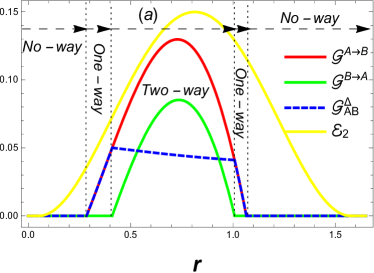
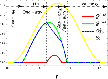
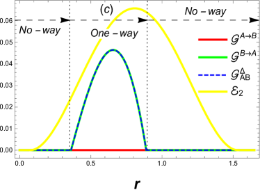
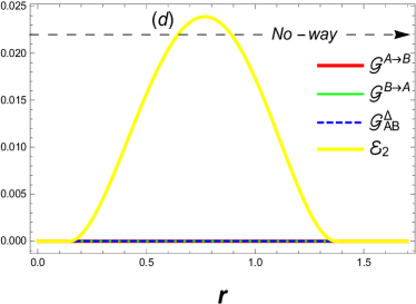
Figure 2: Gaussian steering $\mathcal{G}^{A\rightarrow B}$ (red line), $\mathcal{G}^{B\rightarrow A}$ (green line), steering asymmetry $\mathcal{G}_{AB}^{\Delta}$ (blue dashed line) and GR2E $\mathcal{E}_{2}$ (yellow line) of the two modes $A$ and $B$ versus the squeezing $r$ for various thermal occupations $n_{th,1,2}$. (a) $n_{th,1}=2$, $n_{th,2}=0.5$; (b) $n_{th,1}=0.5$, $n_{th,2}=2$; (c) $n_{th,1}=1$, $n_{th,2}=2$; (d) $n_{th,1}=1$, $n_{th,2}=5$. The optomechanical coupling are $\mathcal{C}_{1}=35$ ($\wp_{1}=12~{}\mathrm{mW}$), $\mathcal{C}_{2}=15$ ($\wp_{2}=5~{}\mathrm{mW}$) [50]. In panel (c), the states of the two modes $A$ and $B$ are entangled, however, they are one-way steerable, which reflects genuinely the asymmetry of quantum correlations.

In Fig. 2, we consider the squeezing influence on the steering $\mathcal{G}^{A\rightarrow B}$, $\mathcal{G}^{B\rightarrow A}$ and entanglement $\mathcal{E}_{2}$ of the two mechanical modes $A$ and $B$. The optomechanical cooperativities are fixed as $\mathcal{C}_{1}=35$ and $\mathcal{C}_{2}=15$. It should be noted that from Eq. (21), the condition $\mathcal{C}_{1}\neq\mathcal{C}_{2}$ can be realised for example by choosing identical parameters for the two cavities, except, the lasers powers ($\wp_{1}\neq\wp_{2}$).

Fig. 2 shows that the steerable states are always entangled, while, entangled ones are not necessary steerable. Moreover, we remark that both steering and entanglement undergo the resonance-like behavior under squeezing effects. This can be well understood knowing that the reduced state of two-mode squeezed light is a thermal state with a mean photons number proportional to the squeezing degree $r$ [51]. So, progressive injection of squeezed light increases the photons number in the two cavities, which leads to strong radiation pressure acting on the optomechanical coupling. This enhances entanglement and steering of the two modes $A$ and $B$. On the other hand, steering and entanglement start to decrease after reaching their maximum. Here the explanation is that, in this period the photons number becomes important in the two cavities, and consequently, the thermal noise entering each cavity becomes more aggressive, bring a quantum correlations degradation. Furthermore, Fig. 2 reveals that the steering $\mathcal{G}^{A\rightarrow B}$ and $\mathcal{G}^{B\rightarrow A}$ are more affected than entanglement $\mathcal{E}_{2}$ by thermal noise induced by high squeezing values $r$. In particular, Figs. 2(a)-2(b) show that by interchanging the values of $n_{th,1}$ and $n_{th,2}$, entanglement $\mathcal{E}_{2}$ is not sensitive to such operation, whereas, the steering $\mathcal{G}^{A\rightarrow B}$ and $\mathcal{G}^{B\rightarrow A}$ are strongly affected. On the other hand, Fig. 2(c) shows an interesting situation in which the two mechanical modes $A$ and $B$ are entangled for $0.1<r<1.5$, nonetheless, they are $B\rightarrow A$ one-way steering, which reflects the asymmetry of quantum correlations [3]. Such property could be interpreted as follows: Alice and Bob can perform the same Gaussian measurements on their shared entangled state, however, obtain contradictory results. In other words, Bob can convince Alice that their shared state is entangled, while the converse is not true. This is partly due to the asymmetry introduced in the system, and partly due to the definition of the aspect of steering in terms of the EPR paradox [7, 14].

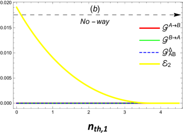
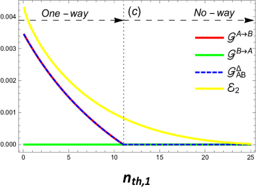
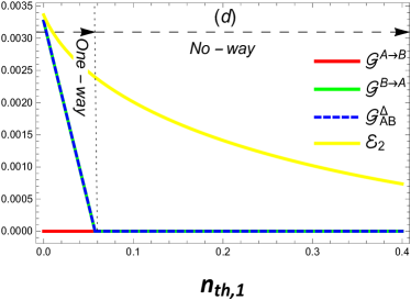
Figure 3: Gaussian steering $\mathcal{G}^{A\rightarrow B}$ (red line), $\mathcal{G}^{B\rightarrow A}$ (green line), steering asymmetry $\mathcal{G}_{AB}^{\Delta}$ (blue dashed line) and GR2E $\mathcal{E}_{2}$ (yellow line) of the two modes $A$ and $B$ versus the thermal occupation $n_{th,1}$ for various values of ${n_{th,2}}$ and squeezing $r$. (a) $r=0.5$, $n_{th,2}=0.1$; (b) $r=0.5$, $n_{th,2}=15$; (c) $r=0.05$, $n_{th,2}=0.01$; (d) $r=0.05$, $n_{th,2}=1.5$. The optomechanical coupling are $\mathcal{C}_{1}=35$ ($\wp_{1}=12~{}\mathrm{mW}$) and $\mathcal{C}_{2}=25$ ($\wp_{2}=8.5~{}\mathrm{mW}$) [50]. We see that steerable states are entangled but not necessarily vice versa.

Next, by choosing different values of the squeezing $r$ and thermal occupations $n_{th,2}$, we consider in Fig. 3, the influence of the thermal occupation $n_{th,1}$ on the steering $\mathcal{G}^{A\rightarrow B}$, $\mathcal{G}^{B\rightarrow A}$ and entanglement $\mathcal{E}_{2}$. The optomechanical cooperativities are $\mathcal{C}_{1}=35$ and $\mathcal{C}_{2}=25$. Fig. 3 shows that with increasing $n_{th,1}$, the steering $\mathcal{G}^{A\rightarrow B}$, $\mathcal{G}^{B\rightarrow A}$ decay strongly than entanglement $\mathcal{E}_{2}$, where they vanish early than entanglement. Afterwards, fixing the squeezing as $r=0.5$, we remark from panel 3(a) that one-way steering and two-way steering can be observed with $n_{th,2}=0.1$, while, in panel 3(b) with $n_{th,2}=15$, the steerability is not authorized in any direction ($\mathcal{G}^{A\rightarrow B}=\mathcal{G}^{B\rightarrow A}=0$) although that the two modes $A$ and $B$ are entangled. This indicates that quantum steering is more fragile than entanglement against thermal noises. Now, fixing the squeezing as $r=0.05$, we remark in panel 3(c) that for $n_{th,2}=0.01$, the two mechanical modes $A$ and $B$ are $A\rightarrow B$ one-way steerable, in contrast, they are $B\rightarrow A$ one-way steerable for $n_{th,2}=1.5$ in panel 3(d). This shows clearly that the steering of the two modes $A$ and $B$ can be oriented by controlling the thermal effects.
From Fig. 3, it is seen that $\mathcal{G}^{A\rightarrow B}$, $\mathcal{G}^{B\rightarrow A}$ and $\mathcal{E}_{2}$ have the same behavior under the thermal effects,i.e. with increasing of $n_{th,1}$, the steering $\mathcal{G}^{A\rightarrow B}$, $\mathcal{G}^{B\rightarrow A}$ decrease with decreasing of entanglement $\mathcal{E}_{2}$. In fact, such result is not general, where it has been shown more recently that the decrease of entanglement does not necessarily mean the decrease of steering [27]. Moreover, Fig. 3 shows that the steerable states are always entangled, whereas, entangled ones are not necessarily steerable, which indicates that nonzero degree of entanglement is indispensable for steering. Further, Figs. 3(c)-3(d) show genuine one-way steering of the two modes $A$ and $B$, indicating that bipartite quantum correlations are not symmetric in general,i.e. quantum correlations measured from $A\rightarrow B$ and from $B\rightarrow A$ do not necessarily coincide. Interesting, Fig. 3 shows that the steering $\mathcal{G}^{A\rightarrow B}$ and $\mathcal{G}^{B\rightarrow A}$ are strongly sensitive to the thermal noise than entanglement $\mathcal{E}_{2}$, having a tendency to vanish rapidly with increasing temperature.
Notice that one-way steering observed in Figs. 2-3, answers genuinely the question raised by Wiseman et al, i.e. is then whether there exists bipartite entangled states which are one-way steerable [3]. This most intriguing feature of quantum correlations, has been expected to play a crucial role in quantum information science, where it can be employed to guarantee secure quantum communication [6].

Overall, Figs. 2-3 show that the steering $\mathcal{G}^{A\rightarrow B}$ and $\mathcal{G}^{B\rightarrow A}$ remain upper bounded by GR2E $\mathcal{E}_{2}$, moreover, the steering asymmetry $\mathcal{G}_{AB}^{\Delta}$ is always less than $\ln 2$, it is maximal when the state is one-way steerable and it decreases with increasing steerability in either way, which is consistent with [14].

4 Conclusions

In an optomechanical system fed by squeezed light and driven in the red sideband, stationary Gaussian steering of two mechanical modes $A$ and $B$ is studied. In the resolved sideband limit, the steady-state covariance matrix describing the two considered modes is calculated. We showed that in the quantum state transfer regime, Gaussian steering can be generated, while, under influence of thermal effects (squeezing and temperature), Gaussian one-way steering is occurred genuinely in Figs. 2(c)-3[(c)-(d)] and over two phases separated by two-way steering behavior in Figs. 2[(a)-(b)]. The scenarios illustrated in Figs. 2(c)-3[(c)-(d)], where the two modes $A$ and $B$ are entangled, however, exhibiting genuine one-way steering, reflect the asymmetric property of quantum correlations,i.e. for a bipartite quantum state $\varrho_{AB}$, quantum correlations measured from $A\rightarrow B$ and from $B\rightarrow A$ do not necessarily coincide [3]. A comparison study between the steering of the two modes $A$ and $B$ with their GR2E $\mathcal{E}_{2}$ showed on the one hand, that both steering and entanglement suffer from a sudden death-like phenomenon with early vanishing of steering in different conditions. On the other hand, Gaussian steering is found stronger than entanglement, however, remains constantly upper bounded by Gaussian Rényi-2 entanglement, and has a tendency to decay rapidly to zero under thermal noises. Finally, the steering asymmetry $\mathcal{G}_{AB}^{\Delta}$ is found always less than ln2, reaches its maximum when the two modes $A$ and $B$ are one-way steerable, and it decreases with increasing steerability in either directions, which is consistent with [14]. This work may contribute to the understanding of the behavior of asymmetric quantum correlations in dissipative-noisy optomechanical systems, which has immediate applications in quantum information processing and communication.

References

• [1] A. Einstein, B. Podolsky, and N. Rosen, Phys. Rev. 47, 777 (1935).
• [2] E. Schrödinger, Math. Proc. Cambridge Philos. Soc. 31, 555 (1935); E. Schrödinger, Math. Proc. Cambridge Philos. Soc. 32, 446 (1936).
• [3] H. M.Wiseman, S. J. Jones, and A. C. Doherty, Phys. Rev. Lett. 98, 140402 (2007).
• [4] J. S. Bell, Physics 1, 195 (1964).
• [5] R. Horodecki, P. Horodecki, M. Horodecki, and K. Horodecki, Rev. Mod. Phys. 81, 865 (2009).
• [6] D. Saunders, S. Jones, H.Wiseman, and G. Pryde, Nature Phys. 6, 845 (2010); A. J. Bennet, D. A. Evans, D. J. Saunders, C. Branciard, E. G. Cavalcanti, H. M. Wiseman, and G. J. Pryde, Phys. Rev. X 2, 031003 (2012).
• [7] M.D. Reid, Phys. Rev. A 40, 913 (1989).
• [8] Z. Y. Ou, S. F. Pereira, H. J. Kimble, and K. C. Peng, Phys. Rev. Lett. 68, 3663 (1992).
• [9] E. G. Cavalcanti, S. J. Jones, H. M. Wiseman, and M. D. Reid, Phys. Rev. A 80, 032112 (2009); I. Kogias, P. Skrzypczyk, D. Cavalcanti, A. Acín, and G. Adesso, Phys. Rev. Lett. 115, 210401 (2015); H. Zhu, M. Hayashi, and L. Chen, Phys. Rev. Lett. 116, 070403 (2016).
• [10] N.Brunner, D.Cavalcanti, S.Pironio, V.Scarani, and S.Wehner, Rev. Mod. Phys. 86, 419 (2014).
• [11] I. Kogias, G. Adesso, J. Opt. Soc. Am. B 32, A27 (2015).
• [12] P. Skrzypczyk, M. Navascués, and D. Cavalcanti, Phys. Rev. Lett. 112, 180404 (2014).
• [13] M. Piani and J. Watrous, Phys. Rev. Lett. 114, 060404 (2015).
• [14] I. Kogias, A. R. Lee, S. Ragy, G. Adesso, Phys. Rev. Lett. 114, 060403 (2015).
• [15] M. K. Olsen, Phys. Rev. Lett. 119, 160501 (2017).
• [16] X.Deng, Y.Xiang, C. Tian, G. Adesso, Q.He, Q.Gong, X.Su, C.Xie and K. Peng, Phys. Rev. Lett. 118, 230501 (2017); J.E. Qars, M. Daoud and R.A. Laamara. Eur. Phys. J. D 71, 122 (2017).
• [17] B. Wittmann, S.Ramelow, F.Steinlechner, N.K. Langford, N. Brunner, H.M. Wiseman, R.Ursin and A. Zeilinger, New J. Phys. 14, 053030 (2012); K.Sun, X.-J. Ye, J.-S. Xu, X.-Y. Xu, J.-S.Tang, Y.-C.Wu, J.-L. Chen, C.-F. Li, and G.-C.Guo, Phys. Rev. Lett. 116, 160404 (2016); S.Kocsis, M.J. W. Hall, A.J. Bennet, D.J. Saunders and G. J. E. Pryde, Nat. Commun 6, 5886 (2015).
• [18] D. A. Evans and H. M. Wiseman, Phys. Rev. A 90, 012114 (2014).
• [19] J. Bowles, T. Vértesi, M. T. Quintino, and N. Brunner, Phys. Rev. Lett. 112, 200402 (2014).
• [20] S. L. W. Midgley, A. J. Ferris, and M. K. Olsen, Phys. Rev. A 81, 022101 (2010).
• [21] S. Wollmann, N. Walk, A. J. Bennet, H. M. Wiseman, and G. J. Pryde, Phys. Rev. Lett. 116, 160403 (2016).
• [22] C. Branciard, E. G. Cavalcanti, S. P. Walborn, V. Scarani, and H. M. Wiseman, Phys. Rev. A 85, 010301 (2012); I. Kogias, Y. Xiang, Q. He, and G. Adesso, Phys. Rev. A 95, 012315 (2017).
• [23] Q. He, L. Rosales-Zárate, G. Adesso, and M. D. Reid, Phys. Rev. Lett. 115, 180502 (2015).
• [24] V. Händchen, T. Eberle, S. Steinlechner, A. Samblowski, T. Franz, R. F. Werner and R. Schnabel, Nature Photonics 6, 596 (2012).
• [25] S. Armstrong, M. Wang, R.Y. Teh, Q. Gong, Q. He, J. Janousek, H.-A. Bachor, M.D. Reid and P.K. Lam, Nat. Phys. 11, 167 (2015).
• [26] S. Kiesewetter, Q.Y. He, P.D. Drummond and M.D. Reid, Phys. Rev. A 90, 043805 (2014).
• [27] H. Tan, W. Deng, Q. Wu, and G. Li. Phys. Rev. A 95, 053842 (2017).
• [28] G. Adesso, D. Girolami, and A. Serafini, Phys. Rev. Lett. 109, 190502 (2012).
• [29] P. Meystre, Ann. Phys. 525, 215 (2013).
• [30] M. Aspelmeyer, T.J. Kippenberg and F. Marquardt, Rev. Mod. Phys. 86, 1391 (2014).
• [31] J. D. Teufel, T. Donner, D. Li, J. W. Harlow, M. S. Allman, K. Cicak, A. J. Sirois, J. D. Whittaker, K. W. Lehnert and R. W. Simmonds, Nature (London) 475, 359 (2011).
• [32] G.S. Agarwal and S. Huang, Phys. Rev. A 81, 041803(R) (2010).
• [33] X. -Y. Lü , J. -Q. Liao , L. Tian, F. Nori, Phys. Rev. A 91, 013834(7) (2015).
• [34] W. Marshall, C. Simon, R. Penrose, D. Bouwmeester, Phys. Rev. Lett. 91, 130401 (2003).
• [35] C. F. Ockeloen-Korppi, et al., Phys. Rev. Lett. 117, 140401 (2016).
• [36] T. A. Palomaki, J. D. Teufel, R. W. Simmonds, and K. W. Lehnert, Science 342, 710 (2013); J. El Qars, M. Daoud, Ahl Laamara, Int. J. Quant. Inform. 13, 1550041 (2015); J. El Qars, M. Daoud, R. Ahl Laamara, Int. J. Mod. Phys. B 30, 1650134 (2016); J. El Qars, M. Daoud and R. Ahl Laamaraa, J. Mod. Opt 65, 1584 (2018).
• [37] C. K. Law, Phys. Rev. A 51, 2537 (1995).
• [38] M. Paternostro, L. Mazzola, and J. Li, J. Phys. B: At. Mol. Opt. Phys. 45, 154010 (2012).
• [39] C. Genes, A. Mari, D. Vitali, P. Tombesi, Adv. At. Mol. Opt. Phys. 57, 33 (2009).
• [40] R. Benguria, and M. Kac, Phys. Rev. Lett, 46, 1 (1981).
• [41] A. S. Parkins and H. J. Kimble, J. Opt. B: Quantum Semiclass. Opt. 1 496 (1999).
• [42] Y.-D. Wang, S. Chesi, A. A. Clerk, Phys. Rev. A 91, 013807 (2015).
• [43] P. C. Parks and V. Hahn, Stability Theory. New York: Prentice Hall, 1993.
• [44] T. P. Purdy, P.-L. Yu, R. W. Peterson, N. S. Kampel, and C. A. Regal, Phys. Rev. X 3, 031012 (2013).
• [45] G. Adesso and A. Datta, Phys. Rev. Lett. 105, 030501 (2010).
• [46] G. Adesso and F. Illuminati, Phys. Rev. A 72, 032334 (2005).
• [47] L. Lami, C. Hirche, G. Adesso, and A. Winter, Phys. Rev. Lett. 117, 220502 (2016).
• [48] A. Rényi ”On measures of information and entropy”, Proceedings of the 4th Berkeley Symposium on Mathematics, Statistics and Probability, p 547; 1960.
• [49] G. Giedke, M.M. Wolf, O. Krüger, R.F.Werner and J.I. Cirac, Phys. Rev. Lett. 91, 107901 (2003).
• [50] S. Gröblacher, K. Hammerer, M.R. Vanner and M. Aspelmeyer, Nature(London) 460, 724 (2009).
• [51] L. Mazzola, M. Paternostro, Phys. Rev. A 83, 062335 (2011).