Electromagnetic perturbations of black holes in general relativity coupled to nonlinear electrodynamics: Polar perturbations

Abstract

The axial electromagnetic (EM) perturbations of the black hole (BH) solutions in general relativity coupled to nonlinear electrodynamics (NED) were studied for both electrically and magnetically charged BHs, assuming that the EM perturbations do not alter the spacetime geometry in our preceding paper [Phys. Rev. D 97, 084058 (2018)]. Here, as a continuation of that work, the formalism for the polar EM perturbations of the BHs in general relativity coupled to the NED is presented. We show that the quasinormal modes (QNMs) spectra of polar EM perturbations of the electrically and magnetically charged BHs in the NED are not isospectral, contrary to the case of the standard Reissner-Nordström BHs in the classical linear electrodynamics. It is shown by the detailed study of QNMs properties in the eikonal approximation that the EM perturbations can be a powerful tool to confirm that in the NED light ray does not follow the null geodesics of the spacetime. By specifying the NED model and comparing axial and polar EM perturbations of the electrically and magnetically charged BHs, it is shown that QNM spectra of the axial EM perturbations of magnetically (electrically) charged BH and polar EM perturbations of the electrically (magnetically) charged BH are isospectral, i.e., $\omega_{mag}^{ax}\approx\omega_{el}^{pol}$ ($\omega_{mag}^{pol}\approx\omega_{el}^{ax}$).

I Introduction

Black holes (BHs) are among the simplest and at the same time most bizarre objects in the Universe – they have only three defining attributes, mass, spin, and electric (or magnetic) charge, according to the no-hair theorem Misner et al. (1973), and there is a spacetime singularity in their interior that is enclosed by an event horizon according to the cosmic censorship Penrose (1969). By listing those three parameters accordingly, one can depict a complete portrait of the BH environment. However, we do not yet have a good enough theory of gravity to explain and describe the spacetime singularity. Therefore, special interests have been raised in coupling general relativity (GR) to another fundamental field theories, such as nonlinear electrodynamics (NED) , to obtain the singularity-free BH solutions Ayón-Beato and García (1998, 2000); Bronnikov (2001); Dymnikova (2004); Dymnikova and Galaktionov (2015); Rodrigues et al. (2018). The generic class of singular and singularity-free BH solutions in GR coupled to the NED is presented in Ref. Fan and Wang (2016) and refined in Refs. Bronnikov (2017); Toshmatov et al. (2018a). Such singularity-free BHs are called regular BHs.

Although BHs cannot be seen directly, one can guess their presence in the particular place of the space by measuring their strong gravity effects on the surrounding objects: mass estimates from test objects orbiting or spiraling into a BH, gravitational lens effects, and radiation emitted by the surrounding matter. Apart from these effects, we can “hear” their collisions representing the final stage of the evolution of the close BH binaries. As sound waves disturb the air to make noise, gravitational waves (GWs) disturb the fabric of spacetime to push and pull matter, as recently LIGO and VIRGO global experiments have directly detected the GWs from the coalescence of two BHs The LIGO Scientific Collaboration and the Virgo Collaboration (2016). The coalescence of two BHs can be divided into three stages: the inspiral, merger and ringdown. Each phase can be calculated by different means. The inspiral can be studied analytically within the post-Newtonian approximation, while the merger is directly computable by using the numerical relativity only. Finally, the ringdown phase describes relaxation of the final object to an equilibrium state by emitting GWs in so-called quasinormal modes (QNMs), the frequencies of this are complex, giving thus also damping of the oscillations. This phase can be also calculated analytically via perturbation theory (see Refs. Kokkotas and Schmidt (1999); Nagar and Rezzolla (2005); Berti et al. (2009); Konoplya and Zhidenko (2011) and references therein).

In the recent preceding paper Toshmatov et al. (2018b), we studied the behavior of the dynamical response of the spherically symmetric, magnetically and/or electrically charged BHs representing exact solutions of coupled Einstein’s gravity and the NED to the axial electromagnetic (EM) perturbations, assuming the EM perturbations do not alter the spacetime geometry. One of the main reasons for the topic was to determine whether it is possible to distinguish the BHs related to the NED from the BHs related to the standard linear electrodynamics (LED) from their response to the EM perturbations. In that paper we showed that i) the axial EM perturbations of in the NED BHs give different potentials and, consequently, different QNM spectra, in comparison with those related to the RN BHs governed by the standard LED, since it is well known from Refs. Chaverra et al. (2016); Moreno and Sarbach (2003); Toshmatov et al. (2018b) that the QNMs of the EM perturbations of the electrically and magnetically charged RN BHs are isospectral, with identical effective potentials; ii) in the eikonal (large multipole numbers) regime, the QNMs of the NED BHs are determined by the unstable circular photon orbits determined by the given geometry, i.e., by unstable circular null geodesics determined by the effective (or optical) geometry, since in the NED light ray does not follow the null geodesics of the spacetime Novello et al. (2000, 2001); Obukhov and Rubilar (2002); Bretón and López (2016); de Oliveira Costa and Perez Bergliaffa (2009); Stuchlík and Schee (2015); Schee and Stuchlík (2015, 2016). It should be noted that one of the outstanding pioneering works devoted to the study of the perturbations of the one-parameter family of Lagrangian densities that yields static, spherically symmetric magnetically charged BH solutions in the NED is the paper Chaverra et al. (2016) that overlaps some important results of the present paper and Ref. Toshmatov et al. (2018b), despite the different models that were used. In that paper the following very important results have been presented: i) A stability analysis has been presented. ii) By studying the QNM spectra it has been shown that the even-parity and odd-parity perturbations are not isospectral in the NED. iii) For the eikonal limit it has been shown that the unstable circular photon orbits of the spacetime plays an important role.

In this paper, as a continuation of our preceding paper Toshmatov et al. (2018b), we study within this framework the polar EM perturbations of the spherically symmetric, magnetically and electrically charged BHs representing exact solutions of coupled Einstein’s gravity (GR) and NED. The paper is organized as follows. In Sec. II we review the equations of motion governing a self-gravitating, NED configuration and discuss spherically symmetric, magnetically and electrically charged BH solutions. In Sec. III we demonstrate the polar EM perturbations of the electrically and magnetically charged, spherically symmetric NED BHs. In Sec. IV we study the QNMs of the electrically charged BHs in the large multipole numbers limit. We apply the obtained formalism for the specific type of BHs in GR coupled to the NED, calculate their QNMs in comparison with the ones of the Schwarzschild and RN BHs in Sec. V. Finally, in Sec. VI we summarize the main results. In this paper we mainly use the natural units $\hbar=c=G=1$. Furthermore, we adopt $(-,+,+,+)$ convention for the signature of the metric.

II BH solutions in GR coupled to NED

In general in the case of GR coupled to NED, the action is given by

$$S=\frac{1}{16\pi}\int d^{4}x\sqrt{-g}\left(R-\mathscr{L}\right)\ ,$$ (1)

where $g$ is the determinant of the metric tensor, $R$ is the Ricci scalar, and $\mathscr{L}$ is the Lagrangian density describing the NED theory that depends on $\mathscr{L}=\mathscr{L}(F\equiv F_{\mu\nu}F^{\mu\nu})$, with $F_{\mu\nu}=\partial_{\mu}A_{\nu}-\partial_{\nu}A_{\mu}$. Since $F_{\mu\nu}$ is antisymmetric, it has only six nonzero components.

The covariant equations of motion are written in the form

$$G_{\mu\nu}=T_{\mu\nu},$$ (2)

$$\nabla_{\nu}\left(\mathscr{L}_{F}F^{\mu\nu}\right)=0\ ,$$ (3)

where $G_{\mu\nu}=R_{\mu\nu}-Rg_{\mu\nu}/2$ and $T_{\mu\nu}$ are the Einstein tensor and the energy-momentum tensor of the NED field, respectively. The energy-momentum tensor of the NED is determined by the relation

$$T_{\mu\nu}=2\left(\mathscr{L}_{F}F_{\mu}^{\alpha}F_{\nu\alpha}-\frac{1}{4}g_{\mu\nu}\mathscr{L}\right)\ ,$$ (4)

where $\mathscr{L}_{F}=\partial_{F}\mathscr{L}$.

Let us consider the line element of the static, spherically symmetric BH is given in the form

$$ds^{2}=-f(r)dt^{2}+\frac{dr^{2}}{f(r)}+r^{2}\left(d\theta^{2}+\sin^{2}\theta d\phi^{2}\right)\ ,$$ (5)

where GR and NED evaluate the lapse function $f(r)$. The line element (5) satisfies the symmetry $G_{t}^{t}=G_{r}^{r}$.

In general, the EM 4-potential can be written in the following form:

$$\bar{A}_{\mu}=\varphi(r)\delta_{\mu}^{t}-Q_{m}\cos\theta\delta_{\mu}^{\phi}\ ,$$ (6)

where $\varphi(r)$ and $Q_{m}$ are the electric potential and the total magnetic charge, respectively. Below based on the method of Bronnikov Bronnikov (2001) we briefly demonstrate the formalism of construction of electrically and magnetically charged BHs in GR coupled to the NED.

Since the formalism of construction of the electrically and magnetically charged BHs in GR coupled to the NED has already been presented in Bronnikov (2001); Fan and Wang (2016); Toshmatov et al. (2018b), we do not report the whole procedure in detail, instead, we briefly mention some key moments.

The electrically charged BH solution with the ansatz $\bar{A}_{t}=\varphi(r)$, and the EM field strength $F=-2\varphi^{\prime 2}$, can be constructed by solving the Einstein field equations (2) as

$$\mathscr{L}=\frac{2m^{\prime\prime}}{r},$$ (7)

$$\mathscr{L}_{F}=\frac{2m^{\prime}-rm^{\prime\prime}}{2r^{2}\varphi^{\prime 2}}\ ,$$ (8)

where $m$ is the radially and EM field dependent mass function of the Schwarzschild-like BHs, related to the metric function as

$$f(r)=1-\frac{2m(r)}{r}\ .$$ (9)

From Eqs. (7) and (8) one can easily notice that if $m(r)=M$, the Lagrangian density of the NED vanishes, $\mathscr{L}=0$, and one arrives at the Schwarzschild solution of GR. The total electric charge inside the sphere with radius $r$ is found by equations of motion (3) as

$$Q_{e}=r^{2}\mathscr{L}_{F}\varphi^{\prime}\ .$$ (10)

By substituting (8) to (10), and solving the differential equation with respect to the electric potential $\varphi(r)$, one obtains the expression for the electric potential as

$$\varphi=\frac{3m-rm^{\prime}}{2Q_{e}}+C\ ,$$ (11)

where $C$ is an integration constant. If one considers the EM field is linear, $\mathscr{L}=F$ (or $\mathscr{L}_{F}=1$), the differential equation (7) (or (8)) gives the RN BH spacetime with mass function $m(r)=M+Q_{e}^{2}/2r$, and corresponding electric potential (11) takes the form $\varphi=Q_{e}/r$.

The magnetically charged spherically symmetric BH solution with the ansatz $\bar{A}_{\phi}=-Q_{m}\cos\theta$ and the EM field strength $F=2Q_{m}^{2}/r^{4}$ can be constructed by solving the Einstein field equations (2) as

$$\mathscr{L}=\frac{4m^{\prime}}{r^{2}}\ ,$$ (12)

$$\mathscr{L}_{F}=\frac{r^{2}(2m^{\prime}-rm^{\prime\prime})}{2Q_{m}^{2}}\ .$$ (13)

If one considers the EM field is linear, $\mathscr{L}=F$ (or $\mathscr{L}_{F}=1$), the differential equation (12) (or (13)) gives the RN BH spacetime with mass function $m(r)=M+Q_{e}^{2}/2r$.

By choosing the mass function related to the electric or magnetic fields as presented above, one can construct BH solutions in GR coupled to the NED. One more important property of the NED is that the NED can eliminate the curvature singularity (divergence of the curvature) of the spacetime. For details, see Refs. Fan and Wang (2016); Toshmatov et al. (2018b).

III Polar EM perturbations of BHs in GR coupled to the NED

In this section we study polar EM perturbations of BHs in NED by introducing the polar EM perturbations into gauge potential (6) as

$$A_{\mu}=\bar{A}_{\mu}+\delta A_{\mu}\ ,$$ (14)

considering the polar perturbations given in the form

$$\delta A_{\mu} = \sum_{\ell,m}\left(\left[\begin{array}[]{c}d^{\ell m}(t,r)Y_{\ell m}(\theta,\phi)\\ h^{\ell m}(t,r)Y_{\ell m}(\theta,\phi)\\ k^{\ell m}(t,r)\partial_{\theta}Y_{\ell m}(\theta,\phi)\\ k^{\ell m}(t,r)\partial_{\phi}Y_{\ell m}(\theta,\phi)\\ \end{array}\right]\right)\ ,$$ (19)

where $Y_{\ell m}(\theta,\phi)$ is the spherical harmonic function of degree $\ell$ and order $m$ related to the angular coordinates $\theta$ and $\phi$. In the next subsection we study electrically and magnetically charged BH cases separately.

III.1 Magnetically charged black holes

The EM four-potential of the magnetically charged BH is given as $\bar{A}_{\mu}=-Q_{m}\cos\theta\delta_{\mu}^{\phi}$. Then, nonzero components of the EM field tensor are given as

$$F_{tr} =\left(\partial_{t}h^{\ell m}-\partial_{r}d^{\ell m}\right)Y_{\ell m}\ ,$$

$$F_{t\theta} =\left(\partial_{t}k^{\ell m}-d^{\ell m}\right)\partial_{\theta}Y_{\ell m}\ ,$$

$$F_{t\phi} =\left(\partial_{t}k^{\ell m}-d^{\ell m}\right)\partial_{\phi}Y_{\ell m}\ ,$$

$$F_{r\theta} =(\partial_{r}k^{\ell m}-h^{\ell m})\partial_{\theta}Y_{\ell m}\ ,$$ (20)

$$F_{r\phi} =(\partial_{r}k^{\ell m}-h^{\ell m})\partial_{\phi}Y_{\ell m}\ ,$$

$$F_{\theta\phi} =Q_{m}\sin\theta\ .$$

The contravariant nonzero components of the EM field tensor are written using the relation $F^{\mu\nu}=g^{\mu\alpha}g^{\nu\beta}F_{\alpha\beta}$ as

$$F_{tr} =-\left(\partial_{t}h^{\ell m}-\partial_{r}d^{\ell m}\right)Y_{\ell m}\ ,$$

$$F_{t\theta} =-\frac{1}{r^{2}f}\left(\partial_{t}k^{\ell m}-d^{\ell m}\right)\partial_{\theta}Y_{\ell m}\ ,$$

$$F_{t\phi} =-\frac{1}{r^{2}f\sin^{2}\theta}\left(\partial_{t}k^{\ell m}-d^{\ell m}\right)\partial_{\phi}Y_{\ell m}\ ,$$

$$F_{r\theta} =\frac{f}{r^{2}}(\partial_{r}k^{\ell m}-h^{\ell m})\partial_{\theta}Y_{\ell m}\ ,$$ (21)

$$F_{r\phi} =\frac{f}{r^{2}\sin^{2}\theta}(\partial_{r}k^{\ell m}-h^{\ell m})\partial_{\phi}Y_{\ell m}\ ,$$

$$F_{\theta\phi} =\frac{Q_{m}}{r^{4}\sin\theta}\ .$$

In the linear perturbations (up to the first order) approximation the EM field strength remains unchanged as $F=\bar{F}$, where

$$\bar{F}=\frac{2Q_{m}^{2}}{r^{4}}\ ,$$ (22)

Consequently, the lagrangian density of the NED also remains unchanged in the linear perturbations approximation, $\mathscr{L}_{F}=\bar{\mathscr{L}}_{\bar{F}}$. With the above given expressions one can obtain from (3) the following three independent ordinary differential equations (ODEs):

$$rf\left(2+\frac{r\mathscr{L}_{F}^{\prime}}{\mathscr{L}_{F}}\right)(\partial_{t}h^{\ell m}-\partial_{r}d^{\ell m})$$ (23)

$$+r^{2}f\partial_{r}(\partial_{t}h^{\ell m}-\partial_{r}d^{\ell m})-\ell(\ell+1)(\partial_{t}k^{\ell m}-d^{\ell m})=0\ ,$$

$$\frac{r^{2}}{f}(\partial_{t}h^{\ell m}-\partial_{r}d^{\ell m})-\ell(\ell+1)(\partial_{t}k^{\ell m}-h^{\ell m})=0\ ,$$ (24)

$$f(f\mathscr{L}_{F})^{\prime}(\partial_{r}k^{\ell m}-h^{\ell m})+f^{2}\mathscr{L}_{F}\partial_{r}(\partial_{r}k^{\ell m}-h^{\ell m})$$

$$+\mathscr{L}_{F}\partial_{t}(d^{\ell m}-\partial_{t}k^{\ell m})=0\ ,$$ (25)

where Eqs. (23), (24), (25) correspond to $\mu=t$, $\mu=r$, $\mu=\theta=\phi$, respectively. By differentiating Eqs. (23) and (24) with respect to $r$ and $t$, respectively, and introducing the tortoise (Regge-Wheeler) coordinate, $dx=dr/f$, and new variable

$$\Psi^{\ell m}(t,r)=\frac{1}{r^{2}\sqrt{\mathscr{L}_{F}}}(\partial_{t}h^{\ell m}-\partial_{r}d^{\ell m})\ ,$$ (26)

one arrives at the well-known wave equation 

$$\left[-\frac{\partial^{2}}{\partial t^{2}}+\frac{\partial^{2}}{\partial x^{2}}-V_{mag}^{pol}(r)\right]\Psi(t,r)=0\ ,$$ (27)

where the effective potential is defined by the expression

$$V_{mag}^{pol}(r)=f\left[\frac{\ell(\ell+1)}{r^{2}}-\frac{3f\mathscr{L}_{F}^{\prime 2}-2\mathscr{L}_{F}\left(f\mathscr{L}_{F}^{\prime}\right)^{\prime}}{4\mathscr{L}_{F}^{2}}\right]\ .$$ (28)

If the EM field is linear, $\mathscr{L}_{F}=1$, then, one recovers the well-known effective potential $V_{mag}^{pol}=f\ell(\ell+1)/r^{2}$ which corresponds to the standard RN and other BHs which are not related to the electrodynamics ($\mathscr{L}_{F}=0$) Toshmatov et al. (2016, 2015).

III.2 Electrically charged black holes

The EM four-potential of the electrically charged BH is given as $\bar{A}_{\mu}=\varphi(r)\delta_{\mu}^{t}$. Then, nonzero components of the EM field tensor are given as

$$F_{tr} =-\varphi^{\prime}+\left(\partial_{t}h^{\ell m}-\partial_{r}d^{\ell m}\right)Y_{\ell m}\ ,$$

$$F_{t\theta} =\left(\partial_{t}k^{\ell m}-d^{\ell m}\right)\partial_{\theta}Y_{\ell m}\ ,$$

$$F_{t\phi} =\left(\partial_{t}k^{\ell m}-d^{\ell m}\right)\partial_{\phi}Y_{\ell m}\ ,$$ (29)

$$F_{r\theta} =(\partial_{r}k^{\ell m}-h^{\ell m})\partial_{\theta}Y_{\ell m}\ ,$$

$$F_{r\phi} =(\partial_{r}k^{\ell m}-h^{\ell m})\partial_{\phi}Y_{\ell m}\ ,$$

The contravariant nonzero components of the EM field tensor are written using the relation $F^{\mu\nu}=g^{\mu\alpha}g^{\nu\beta}F_{\alpha\beta}$ as

$$F^{tr} =\varphi^{\prime}-\left(\partial_{t}h^{\ell m}-\partial_{r}d^{\ell m}\right)Y_{\ell m}\ ,$$

$$F^{t\theta} =-\frac{1}{r^{2}f}\left(\partial_{t}k^{\ell m}-d^{\ell m}\right)\partial_{\theta}Y_{\ell m}\ ,$$

$$F^{t\phi} =-\frac{1}{r^{2}f\sin^{2}\theta}\left(\partial_{t}k^{\ell m}-d^{\ell m}\right)\partial_{\phi}Y_{\ell m}\ ,$$ (30)

$$F^{r\theta} =\frac{f}{r^{2}}(\partial_{r}k^{\ell m}-h^{\ell m})\partial_{\theta}Y_{\ell m}\ ,$$

$$F^{r\phi} =\frac{f}{r^{2}\sin^{2}\theta}(\partial_{r}k^{\ell m}-h^{\ell m})\partial_{\phi}Y_{\ell m}\ ,$$

Thus the EM field strength also takes new form as $F=\bar{F}+\delta F$ where

$$\bar{F}=-2\varphi^{\prime 2},\quad\delta F=4\varphi^{\prime}\left(\partial_{t}h^{\ell m}-\partial_{r}d^{\ell m}\right)Y_{\ell m}\ .$$ (31)

Consequently, $\mathscr{L}_{F}$ also changes to $\mathscr{L}_{F}=\bar{\mathscr{L}}_{\bar{F}}+\bar{\mathscr{L}}_{\bar{F}\bar{F}}\delta F$. By using this and the contravariant components of the EM field tensor (III.2) in Eq. (3), one arrives at the following ODEs:

$$\frac{rf[2\bar{\mathscr{L}}_{\bar{F}}+r\bar{\mathscr{L}}_{\bar{F}}^{\prime}-4\varphi^{\prime}\left(r\bar{\mathscr{L}}_{\bar{F}}^{\prime}\varphi^{\prime}+2\bar{\mathscr{L}}_{\bar{F}\bar{F}}(r\varphi^{\prime})^{\prime}\right)]}{\bar{\mathscr{L}}_{\bar{F}}}\left(\partial_{t}h^{\ell m}-\partial_{r}d^{\ell m}\right)$$

$$+r^{2}f(\bar{\mathscr{L}}_{\bar{F}}-4\bar{\mathscr{L}}_{\bar{F}\bar{F}}\varphi^{\prime 2})\partial_{r}\left(\partial_{t}h^{\ell m}-\partial_{r}d^{\ell m}\right)-\ell(\ell+1)(\partial_{t}k^{\ell m}-d^{\ell m})=0\ ,$$ (32)

$$\frac{r^{2}(\bar{\mathscr{L}}_{\bar{F}}-4\bar{\mathscr{L}}_{\bar{F}\bar{F}}\varphi^{\prime 2})}{f\bar{\mathscr{L}}_{\bar{F}}}\partial_{t}\left(\partial_{t}h^{\ell m}-\partial_{r}d^{\ell m}\right)-\ell(\ell+1)(\partial_{r}k^{\ell m}-h^{\ell m})=0\ ,$$ (33)

Differentiating Eqs. (32) and (33) with respect to the coordinates $r$ and $t$, respectively, and subtracting them, one arrives at the well known wave equation

$$\left[-\frac{\partial^{2}}{\partial t^{2}}+\frac{\partial^{2}}{\partial z^{2}}-V_{el}^{pol}(r)\right]\Phi(t,r)=0\ ,$$ (34)

where the new function $\Phi(t,r)$ is introduced and defined by

$$\Phi^{\ell m}(t,r)=\partial_{t}h^{\ell m}-\partial_{r}d^{\ell m}\ ,$$ (35)

and $z$ is newly introduced tortoise-like coordinate, $dz=dr/f\sqrt{\bar{\mathscr{L}}_{\bar{F}}}$. The potential $V_{el}^{pol}$ is given by

$$V_{el}^{pol}(r)=\frac{f}{\left(\bar{\mathscr{L}}_{\bar{F}}-4\bar{\mathscr{L}}_{\bar{F}\bar{F}}\varphi^{\prime 2}\right)}\left[\frac{\bar{\mathscr{L}}_{\bar{F}}\ell(\ell+1)}{r^{2}}-\frac{f^{\prime}A}{4r}-\frac{fB}{16r^{2}\left(\bar{\mathscr{L}}_{\bar{F}}-4\bar{\mathscr{L}}_{\bar{F}\bar{F}}\varphi^{\prime 2}\right)\bar{\mathscr{L}}_{\bar{F}}}\right]\ ,$$ (36)

where

$$A =-8(\bar{\mathscr{L}}_{\bar{F}}-1)\varphi^{\prime}\left[2\bar{\mathscr{L}}_{\bar{F}\bar{F}}(r\varphi^{\prime})^{\prime}+\bar{\mathscr{L}}_{\bar{F}\bar{F}}^{\prime}r\varphi^{\prime}\right]+4\bar{\mathscr{L}}_{\bar{F}}^{2}+\bar{\mathscr{L}}_{\bar{F}}(r\bar{\mathscr{L}}_{\bar{F}}^{\prime}-4)+2r\bar{\mathscr{L}}_{\bar{F}}^{\prime}(2\bar{\mathscr{L}}_{\bar{F}\bar{F}}\varphi^{\prime 2}-1)\ ,$$

$$B =-4\left[r\bar{\mathscr{L}}_{\bar{F}}^{\prime}\left(2\bar{\mathscr{L}}_{\bar{F}\bar{F}}\varphi^{\prime 2}-1\right)+4\varphi^{\prime}\left(r\bar{\mathscr{L}}_{\bar{F}\bar{F}}^{\prime}\varphi^{\prime}+2\bar{\mathscr{L}}_{\bar{F}\bar{F}}(r\varphi^{\prime})^{\prime}\right)\right]\left[r\bar{\mathscr{L}}_{\bar{F}}^{\prime}\left(6\bar{\mathscr{L}}_{\bar{F}\bar{F}}\varphi^{\prime 2}-1\right)+4\varphi^{\prime}\left(r\bar{\mathscr{L}}_{\bar{F}\bar{F}}^{\prime}\varphi^{\prime}+2\bar{\mathscr{L}}_{\bar{F}\bar{F}}(r\varphi^{\prime})^{\prime}\right)\right]$$

$$+8\bar{\mathscr{L}}_{\bar{F}}\left\{4\varphi^{\prime}\left[\bar{\mathscr{L}}_{\bar{F}\bar{F}}\left(\varphi^{\prime}\left(r\left(4\varphi^{\prime 2}\left(r\bar{\mathscr{L}}_{\bar{F}\bar{F}}^{\prime\prime}+4\bar{\mathscr{L}}_{\bar{F}\bar{F}}^{\prime}\right)-r\bar{\mathscr{L}}_{\bar{F}}^{\prime\prime}\right)+4\right)+4r\varphi^{\prime\prime}\left(4r\bar{\mathscr{L}}_{\bar{F}\bar{F}}^{\prime}\varphi^{\prime 2}+1\right)\right)+2\bar{\mathscr{L}}_{\bar{F}\bar{F}}^{2}\varphi^{\prime}\left(\left(r^{2}\bar{\mathscr{L}}_{\bar{F}}^{\prime\prime}+4\right)\varphi^{\prime 2}\right.\right.\right.$$

$$\left.\left.\left.+4r^{2}\varphi^{\prime\prime 2}+4r\varphi^{\prime}\left(r\varphi^{(3)}+4\varphi^{\prime\prime}\right)\right)+2r\bar{\mathscr{L}}_{\bar{F}\bar{F}}^{\prime}\varphi^{\prime}\right]+2r\bar{\mathscr{L}}_{\bar{F}}^{\prime}\left(2r\varphi^{\prime}\left(\bar{\mathscr{L}}_{\bar{F}\bar{F}}^{\prime}\varphi^{\prime}+2\bar{\mathscr{L}}_{\bar{F}\bar{F}}\varphi^{\prime\prime}\right)-1\right)+r^{2}\bar{\mathscr{L}}_{\bar{F}}^{\prime 2}\left(3\bar{\mathscr{L}}_{\bar{F}\bar{F}}\varphi^{\prime 2}-1\right)\right\}$$

$$+4\bar{\mathscr{L}}_{\bar{F}}^{3}\left\{r\left[-r\bar{\mathscr{L}}_{\bar{F}}^{\prime\prime}-4\bar{\mathscr{L}}_{\bar{F}}^{\prime}+8\left(r\bar{\mathscr{L}}_{\bar{F}\bar{F}}^{\prime\prime}\varphi^{\prime 2}+2\bar{\mathscr{L}}_{\bar{F}\bar{F}}^{\prime}\varphi^{\prime}\left(2r\varphi^{\prime\prime}+\varphi^{\prime}\right)+2r\bar{\mathscr{L}}_{\bar{F}\bar{F}}\varphi^{\prime\prime 2}+2\bar{\mathscr{L}}_{\bar{F}\bar{F}}\varphi^{\prime}\left(r\varphi^{(3)}+2\varphi^{\prime\prime}\right)\right)\right]+4\right\}$$

$$+\bar{\mathscr{L}}_{\bar{F}}^{2}\left\{r\left[-8\left(-r\bar{\mathscr{L}}_{\bar{F}}^{\prime\prime}+4\left(4r\bar{\mathscr{L}}_{\bar{F}\bar{F}}\bar{\mathscr{L}}_{\bar{F}\bar{F}}^{\prime\prime}\varphi^{\prime 4}+r\bar{\mathscr{L}}_{\bar{F}\bar{F}}^{\prime\prime}\varphi^{\prime 2}+2r\bar{\mathscr{L}}_{\bar{F}\bar{F}}\varphi^{\prime\prime 2}+8\bar{\mathscr{L}}_{\bar{F}\bar{F}}^{2}\varphi^{\prime 3}\left(r\varphi^{(3)}+2\varphi^{\prime\prime}\right)\right.\right.\right.\right.$$

$$\left.\left.\left.\left.+2\bar{\mathscr{L}}_{\bar{F}\bar{F}}\varphi^{\prime}\left(r\varphi^{(3)}+4\varphi^{\prime\prime}\right)\right)-8r\bar{\mathscr{L}}_{\bar{F}\bar{F}}^{\prime 2}\varphi^{\prime 4}+16\bar{\mathscr{L}}_{\bar{F}\bar{F}}^{\prime}\varphi^{\prime}\left(2\bar{\mathscr{L}}_{\bar{F}\bar{F}}\varphi^{\prime 2}+1\right)\left(r\varphi^{\prime\prime}+\varphi^{\prime}\right)\right)\right.\right.$$

$$\left.\left.+16\bar{\mathscr{L}}_{\bar{F}}^{\prime}\left(-2r\bar{\mathscr{L}}_{\bar{F}\bar{F}}^{\prime}\varphi^{\prime 2}+4\bar{\mathscr{L}}_{\bar{F}\bar{F}}\varphi^{\prime}\left(\varphi^{\prime}-r\varphi^{\prime\prime}\right)+1\right)+r\bar{\mathscr{L}}_{\bar{F}}^{\prime 2}\right]-16\left(8\bar{\mathscr{L}}_{\bar{F}\bar{F}}\varphi^{\prime 2}+1\right)\right\}\ .$$

In the case of the linear EM field, $\bar{\mathscr{L}}_{\bar{F}}=1$, the effective potential (36) turns out the one for the standard RN BHs.

Since solving the wave equation (34) with the potential (36) requires to specify the NED (lagrangian density), we postpone these calculations to the next sections where we plan to present few special models.

IV QNMs of NED BHs from unstable null geodesics

According to Cardoso et al. (2009), the QNMs of any stationary, spherically symmetric and asymptotically flat BHs in any dimensions are determined in the eikonal regime  by the circular null geodesics  namely, the real part of the QN frequencies is determined by angular velocity of the unstable null geodesics, $\Omega_{c}$, while the imaginary part of the QN frequencies is determined by the so-called Lyapunov exponent, $\lambda$ as

$$\omega=\Omega_{c}\ell-i\left(n+\frac{1}{2}\right)|\lambda|\ ,$$ (37)

where $\Omega_{c}$ and $\lambda$ for the spacetime metric (5) are given by the following expressions

$$\Omega_{c}=\sqrt{\frac{f_{c}}{r_{c}^{2}}}\ ,$$ (38)

$$\lambda=\sqrt{-\frac{r_{c}^{2}}{2f_{c}}\left(\frac{d^{2}}{dx^{2}}\frac{f}{r^{2}}\right)|_{r=r_{c}}}\ ,$$ (39)

where $x$ is the tortoise coordinate, $r_{c}$ is radius of the unstable null circular orbit which is determined by the equation $r_{c}f_{c}^{\prime}-2f_{c}=0$. However, in our preceding paper Toshmatov et al. (2018b), we have shown in the study of the axial EM perturbations to the BHs in GR coupled to the NED that the QNMs of any stationary, spherically symmetric and asymptotically flat BHs in the eikonal (large multipole number) regime are not determined by the parameters of the circular null geodesics, instead they are determined by the parameters of the circular photon orbit, since in the NED light ray does not follow the null geodesics Novello et al. (2000, 2001); Obukhov and Rubilar (2002); Bretón and López (2016); de Oliveira Costa and Perez Bergliaffa (2009). Here, we approve that statement by study of the polar EM perturbations. Below we briefly present the procedure.

In the large multipole numbers limit, one can write the effective potential (36) in the following form:

$$V=\ell^{2}\left[\frac{f}{r^{2}}\left(1-\frac{4\bar{\mathscr{L}}_{\bar{F}\bar{F}}\varphi^{\prime 2}}{\bar{\mathscr{L}}_{\bar{F}}}\right)^{-1}+O\left(\frac{1}{\ell}\right)\right]\ ,$$ (40)

The effective metric is constructed as

$$g_{eff}^{\mu\nu}=\bar{\mathscr{L}}_{\bar{F}}g^{\mu\nu}-4\bar{\mathscr{L}}_{\bar{F}\bar{F}}g_{\alpha\beta}\bar{F}^{\mu\beta}\bar{F}^{\alpha\nu}\ .$$ (41)

From (41), one can construct an infinite number of the effective metrics with the conformal factors, such as

$$g^{eff}_{\mu\nu}=\Omega_{1}^{2}diag\left\{-g,\frac{1}{h},r^{2},r^{2}\sin^{2}\theta\right\}\ ,$$ (42)

with

$$g=f\left(1-\frac{4\bar{\mathscr{L}}_{\bar{F}\bar{F}}\varphi^{\prime 2}}{\bar{\mathscr{L}}_{\bar{F}}}\right)^{-1},\quad h=f\left(1-\frac{4\bar{\mathscr{L}}_{\bar{F}\bar{F}}\varphi^{\prime 2}}{\bar{\mathscr{L}}_{\bar{F}}}\right)\ ,$$

or

$$g^{eff}_{\mu\nu}=\Omega_{2}^{2}diag\left\{-f,\frac{1}{f},\tilde{r}^{2},\tilde{r}^{2}\sin^{2}\theta\right\}\ ,$$ (43)

with

$$\tilde{r}=r\left(1-\frac{4\bar{\mathscr{L}}_{\bar{F}\bar{F}}\varphi^{\prime 2}}{\bar{\mathscr{L}}_{\bar{F}}}\right)^{1/2}\ ,$$

where the conformal factors $\Omega_{1}^{2}=1/\bar{\mathscr{L}}_{\bar{F}}$ and $\Omega_{2}^{2}=1/\left(\bar{\mathscr{L}}_{\bar{F}}-4\bar{\mathscr{L}}_{\bar{F}\bar{F}}\varphi^{\prime 2}\right)$. It is well known that the conformal factor $\Omega^{2}$ can be ignored in the EM perturbations Toshmatov et al. (2017) and null geodesics Bambi et al. (2017), since it plays no role in these phenomena. In both (42) and (43) spacetime metrics, the effective potentials for the massless particles can be written as

$$V=g\frac{\ell^{2}}{r^{2}}\ ,\quad or\quad V=f\frac{\ell^{2}}{\tilde{r}^{2}}\ ,$$ (44)

respectively, which are identical with (40). Here, one can find the parameters of the circular massless particle orbit as

$$\Omega_{c}=\sqrt{\frac{g_{c}}{r_{c}^{2}}}\ ,$$ (45)

$$\lambda=\sqrt{\frac{h_{c}}{2r_{c}^{2}}\left(2g_{c}-r_{c}^{2}g_{c}^{\prime\prime}\right)}\ ,$$ (46)

or

$$\Omega_{c}=\sqrt{\frac{f_{c}}{\tilde{r}_{c}^{2}}}\ ,$$ (47)

$$\lambda=\sqrt{\frac{f_{c}}{2\tilde{r}_{c}^{2}}\left(2f_{c}-\tilde{r}_{c}^{2}f_{c}^{\prime\prime}\right)}\ ,$$ (48)

where the radius of the unstable photon orbit $r_{c}$ is determined by the equation $r_{c}g_{c}^{\prime}-2g_{c}=0$ or $\tilde{r}_{c}f_{c}^{\prime}-2f_{c}=0$.

V EM QNMs of the BHs in GR coupled to the NED

In this section we apply the above demonstrated formalism for the new type of BH solutions in GR coupled to the NED derived in Toshmatov et al. (2018a, b) reinterpreting the physical parameters of the spacetime presented in Fan and Wang (2016). Thus, the mass function of the metric function (9) is given as

$$m(r)=M-\frac{q^{3}}{\alpha}\left[1-\frac{r^{\mu}}{(r+q)^{\mu}}\right]\ ,$$ (49)

Where $\mu\geq 3$ provides the spacetime to be regular only if the condition $M=M_{em}\equiv q^{3}/\alpha$ is satisfied. Therefore, the metric function of the new type of regular BH solutions are given as

$$f(r)=1-\frac{2Mr^{\mu-1}}{(r+q)^{\mu}}\ .$$ (50)

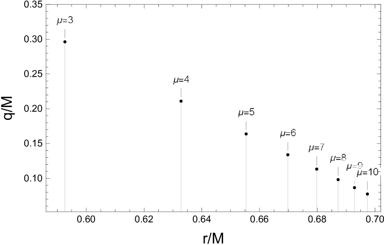
Figure 1: Boundaries of the Maxwellian BHs and no-horizon spacetimes in the parametric space. The black points correspond to the extremal BHs ($r_{ext}/M$, $q_{ext}/M$).

This solution represents the BH with two (inner and outer) horizons, extremal BH with only one degenerate horizon, and no-horizon spacetimes. These all cases depend on the values of parameters $q$ and $\mu$. In Fig. 1 these cases are presented in the parametric space. There shaded regions represent the possible values of the charge parameter for the spacetime to represent BHs.

Let us turn our attention to the EM perturbations of these solutions. Here one should note that the EM perturbations of the solution (50) strongly depend on type of the charge of BHs, i.e., despite the geometry of the magnetically and electrically charged BHs (50) are the same, their Lagrangian densities and consequently, their responses to the EM perturbations are significantly different as their effective potentials (28) and (36) are different as well.

If we consider the BH solution (5) with the mass function (49) is electrically charged, then, the Lagrangian density of it is given by the function

$$\bar{\mathscr{L}}=\frac{2\mu}{\alpha}x^{4}(1+x)^{-\mu-2}((\mu-1)x-2)\ ,\quad x\equiv\frac{q}{r}\ ,$$ (51)

The electric potential is given as

$$\varphi=\frac{\mu}{\sqrt{2\alpha}}x(1+x)^{-\mu-1}(1-(\mu-3)x)\ ,$$ (52)

Then, the EM field strength takes the following form:

$$\bar{F}=-\frac{\mu^{2}}{\alpha}x^{4}(1+x)^{-2\mu-4}((\mu-3)x-4)^{2}\ .$$ (53)

The effective potential of the polar (36) and axial ((34) in the paper Toshmatov et al. (2018b)) EM perturbations of the BH with the mass function (50) are plotted in Fig. 2. We do not report the full expression of these potentials because of their cumbersome forms. Where $\bar{\mathscr{L}}_{\bar{F}}=\bar{\mathscr{L}}^{\prime}/\bar{F}^{\prime}$, $\bar{\mathscr{L}}_{\bar{F}\bar{F}}=\bar{\mathscr{L}}_{\bar{F}}^{\prime}/\bar{F}^{\prime}$.

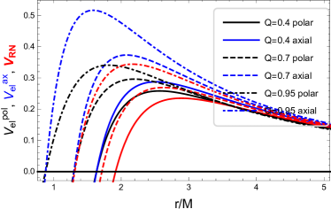
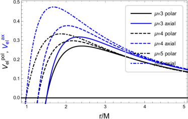
Figure 2: Effective potentials of the polar (black curves, given by the potential (36)) and axial (blue curves, given by the potential (34) of Ref. Toshmatov et al. (2018b)) EM perturbations of the electrically charged regular BHs in comparison with the one of the RN BH (red curves) for the different values of the normalized charge parameter $Q$ (left panel) and $\mu$ (right panel).

Now let us calculate the QNMs of the polar and axial EM perturbations of the electrically charged regular BHs (5) with the mass function (49) and compare them with the standard RN BH in the LED by the sixth order WKB method. Since the possible values of the charge parameters of the regular BH (5) with the mass function (49) and the RN BH are different, in order to facilitate the comparison we turn into the dimensionless normalized charge parameters as $q\rightarrow Qq_{ext}$ with $Q\equiv q/q_{ext}$. After this transformation charge parameters of the both BHs accept the values in the same range as $Q\in[0,1]$. One should note that the polar and axial EM perturbations of the electrically and magnetically charged RN BHs are the same, i.e.., they are isospectral.

$\ell$	$Q$	polar ($\mu=3$)	axial ($\mu=3$)	RN BH	polar ($\mu=4$)	axial ($\mu=4$)
	0	0.2459 - i 0.0931	0.2459 - i 0.0931	0.2459 - i 0.0931	0.2459 - i 0.0931	0.2459 - i 0.0931
1	0.4	0.2689 - i 0.0950	0.2879 - i 0.0970	0.2540 - i 0.0940	0.2687 - i 0.0950	0.2856 - i 0.0967
	0.7	0.2921 - i 0.0946	0.3375 - i 0.0982	0.2752 - i 0.0952	0.2918 - i 0.0945	0.3319 - i 0.0977
	0.95	0.3173 - i 0.0898	0.4105 - i 0.0902	0.3177 - i 0.0904	0.3171 - i 0.0895	0.3988 - i 0.0898
	0	0.4571 - i 0.0951	0.4571 - i 0.0951	0.4571 - i 0.0951	0.4571 - i 0.0951	0.4571 - i 0.0951
2	0.4	0.4952 - i 0.0969	0.5269 - i 0.0987	0.4707 - i 0.0959	0.4949 - i 0.0968	0.5230 - i 0.0985
	0.7	0.5332 - i 0.0966	0.6088 - i 0.0997	0.5056 - i 0.0970	0.5328 - i 0.0965	0.5994 - i 0.0992
	0.95	0.5755 - i 0.0923	0.7292 - i 0.0916	0.5751 - i 0.0927	0.5751 - i 0.0920	0.7097 - i 0.0913
	0	0.6567 - i 0.0956	0.6567 - i 0.0956	0.6567 - i 0.0956	0.6567 - i 0.0956	0.6567 - i 0.0956
3	0.4	0.7101 - i 0.0974	0.7546 - i 0.0992	0.6758 - i 0.0965	0.7097 - i 0.0974	0.7491 - i 0.0990
	0.7	0.7632 - i 0.0971	0.8691 - i 0.1001	0.7245 - i 0.0976	0.7625 - i 0.0970	0.8560 - i 0.0997
	0.95	0.8224 - i 0.0930	1.0374 - i 0.0919	0.8215 - i 0.0933	0.8219 - i 0.0927	1.0100 - i 0.0917

Table 1: Fundamental ($n=0$) QNMs of the polar and axial EM perturbations of the electrically charged BH (5) with the mass function (49) in the NED in comparison with the ones of the RN BHs in the LED.

In Table 1 and Fig. 4 some fundamental QNMs of the axial and polar EM perturbations of the electrically charged BH (5) with the mass function (49) in the NED in comparison with the ones of the RN BHs in the LED are presented for the several values of the electric charge parameter $q$ and nonlinearity degree $\mu$. In Fig. 4 the junctions of the curves correspond to value of the QNMs of the Schwarzschild BH.

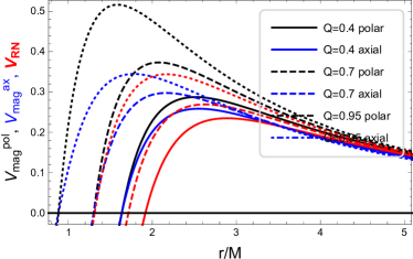
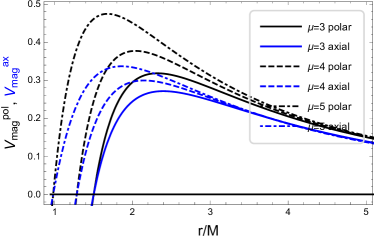
Figure 3: The same as Fig. 2 but for the magnetically charged regular Maxwellian BHs. Where black curves correspond to the potential (28), while the blue curves correspond to the potential (43) of Ref. Toshmatov et al. (2018b).

$\ell$	$Q$	polar ($\mu=3$)	axial ($\mu=3$)	RN BH	polar ($\mu=4$)	axial ($\mu=4$)
	0	0.2459 - i 0.0931	0.2459 - i 0.0931	0.2459 - i 0.0931	0.2459 - i 0.0931	0.2459 - i 0.0931
1	0.4	0.2876 - i 0.0970	0.2691 - i 0.0950	0.2540 - i 0.0940	0.2853 - i 0.0968	0.2689 - i 0.0950
	0.7	0.3366 - i 0.0984	0.2928 - i 0.0945	0.2752 - i 0.0952	0.3311 - i 0.0978	0.2924 - i 0.0943
	0.95	0.4085 - i 0.0907	0.3187 - i 0.0887	0.3177 - i 0.0904	0.3970 - i 0.0900	0.3180 - i 0.0884
	0	0.4571 - i 0.0951	0.4571 - i 0.0951	0.4571 - i 0.0951	0.4571 - i 0.0951	0.4571 - i 0.0951
2	0.4	0.5268 - i 0.0987	0.4953 - i 0.0969	0.4707 - i 0.0959	0.5230 - i 0.0985	0.4950 - i 0.0968
	0.7	0.6084 - i 0.0997	0.5336 - i 0.0964	0.5056 - i 0.0970	0.5991 - i 0.0993	0.5330 - i 0.0964
	0.95	0.7281 - i 0.0917	0.5760 - i 0.0918	0.5751 - i 0.0927	0.7086 - i 0.0914	0.5753 - i 0.0916
	0	0.6567 - i 0.0956	0.6567 - i 0.0956	0.6567 - i 0.0956	0.6567 - i 0.0956	0.6567 - i 0.0956
3	0.4	0.7545 - i 0.0992	0.7102 - i 0.0974	0.6758 - i 0.0965	0.7491 - i 0.0990	0.7097 - i 0.0974
	0.7	0.8688 - i 0.1001	0.7634 - i 0.0970	0.7245 - i 0.0976	0.8557 - i 0.0997	0.7626 - i 0.0969
	0.95	1.0366 - i 0.0920	0.8227 - i 0.0927	0.8215 - i 0.0933	1.0093 - i 0.0917	0.8219 - i 0.0925

Table 2: The same as Table 1 but for the magnetically charged Maxwellian BHs.

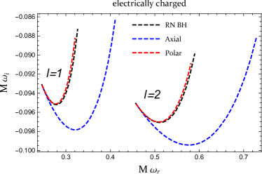
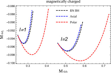
Figure 4: $\ell=1$ and $\ell=2$ fundamental QNMs of the EM perturbations of the electrically and magnetically charged (Maxwellian) regular BH in the NED and RN BH in the LED for the whole range of the charge parameter $Q\in[0,1]$. Where junctions of the curves correspond to the ones of the Schwarzschild BH ($Q=0$).

If the magnetically charged BH solutions in the GR coupled to the NED (5) with the mass function (49) are considered, we will not present the Lagrangian densities of that solutions since in our previous paper Toshmatov et al. (2018b) they have been demonstrated. Since in this case the Lagrangian density tends to the Maxwell one in weak field regime, we called it as Maxwellian BHs. Moreover, again we do not report the full expressions of the effective potentials of the polar and axial EM perturbations due to their cumbersome forms, instead we show their forms in Fig. 3. In Table 2 and Fig. 4 the QNMs of the polar and axial EM perturbations of the magnetically charged regular BHs in the NED and RN BH in the LED have been presented.

One can see from Tables 1, 2 and Fig. 4 that with increasing the value of the charge parameters the frequencies of the real oscillations of the EM perturbations of the BHs in the NED and LED increase, while the damping rates of these oscillations increase up to $Q\approx 0.7$, then they decrease dramatically. One of the momentous results of this paper is that if the geometry (spacetime) of the electrically and magnetically charged BHs in the NED are the same, the axial EM perturbations of the magnetically charged and polar EM perturbations of the electrically charged BHs are isospectral, while axial EM perturbations of the electrically charged and polar EM perturbations of the magnetically charged BHs are isospectral as

$$\omega_{mag}^{ax}\approx\omega_{el}^{pol},\qquad\omega_{mag}^{pol}\approx\omega_{el}^{ax},$$ (54)

i.e., without specifying the type of the EM perturbations, one cannot recognize if the BH in the GR coupled to the NED is magnetically or electrically charged, and vice versa, from the QNM spectra.

Moreover, an increase in the value of parameter $\mu$ decreases both real and imaginary parts of the QNMs. Thus, one can conclude that the EM perturbations of highly charged BHs or BHs in the NED with big $\mu$ parameters live longer. Furthermore, the EM perturbations of the BH in the LED (RN BH) live longer than in the NED for the small and intermediate values of the charge. However, for the large values of the charge parameter the EM perturbations of the BH in the NED live longer.

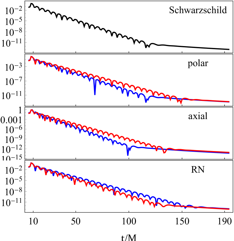
Figure 5: Semilog plot of the temporal evolution of $\ell=2$ axial and polar EM perturbations of the electrically charged BH (5) with the mass function (49) in the NED in comparison with the RN BH in the LED and the Schwarzschild BH. Where blue and red curves correspond to $Q=0.7$ and $Q=0.95$, respectively.

In Fig. 5 time domain profile of the EM perturbations of the electrically charged BH (5) with the mass function (49) for the different values of the charge parameter have been presented in comparison with the ones of the Schwarzschild and RN BHs. Since from Fig. 4 and Eq. (54) it can be realized easily that the time domain profile of the EM perturbations of the magnetically charged BH (5) with the mass function (49) for the different values of the charge parameter is the same as Fig. 5 only if axial and polar epilogs are interchanged.

VI Conclusion

The present paper represents a continuation of our recent paper Toshmatov et al. (2018b) devoted to the study of the axial EM perturbations of the BHs in GR coupled to the NED, considered for both electrically and magnetically charged BHs under assumption that the EM perturbations do not alter the spacetime geometry. The detailed analysis of the polar EM perturbations performed in the present study have demonstrated that the polar EM perturbations of the NED BHs give different effective potentials and consequently, different results for the QNMs, as compared to those related to the standard RN BHs in the LED. It is well known that both the axial and polar EM perturbations of the electrically and magnetically charged BHs in the LED (RN) are isospectral, i.e., they have the same effective potentials and QNMs. However, in the case of the BHs in the NED, electrically and magnetically charged BHs have different potentials and different QNM spectra.

Moreover, we have shown in the detailed study of the QNMs properties in the eikonal (large multipole numbers) approximation that the EM perturbations can play a powerful tool to confirm that the light ray does not follow the null geodesics of the spacetime in the NED. To be more precise, in the paper Cardoso et al. (2009) it was formulated that in the eikonal regime QNMs are determined by the parameters of the unstable circular null geodesics. In this paper, analysis of the polar EM perturbations (as axial EM perturbations in Toshmatov et al. (2018b)) have shown that the QNMs of the BHs in the NED are determined by the unstable circular photon orbits determined by the effective geometry, as in the case of the axial perturbations.

As a special case we have studied the polar EM perturbations of the electrically and magnetically charged new BH solutions in GR coupled to the NED Toshmatov et al. (2018a) in comparison with the ones of the RN BH in the LED and Schwarzschild BH. Moreover, we have compared the obtained polar EM perturbations with the known axial EM perturbations Toshmatov et al. (2018b). The detailed analysis of the QNM spectra of the axial and polar EM perturbations of the electrically and magnetically charged BHs provide justification for fundamental statement that the magnetically and electrically charged BH spacetimes in the GR coupled to the NED are dual to each other, i.e. axial EM perturbations of magnetically (electrically) charged BH and polar EM perturbations of the electrically (magnetically) charged BH are isospectral, i.e. $\omega_{mag}^{ax}\approx\omega_{el}^{pol}$ ($\omega_{mag}^{pol}\approx\omega_{el}^{ax}$).

References

- Misner et al. (1973) C. W. Misner, K. S. Thorne, and J. A. Wheeler, San Francisco: W.H. Freeman and Co., 1973 (1973).
- Penrose (1969) R. Penrose, Nuovo Cimento Rivista Serie 1 (1969).
- Ayón-Beato and García (1998) E. Ayón-Beato and A. García, Phys. Rev. Lett. 80, 5056 (1998), gr-qc/9911046 .
- Ayón-Beato and García (2000) E. Ayón-Beato and A. García, Phys. Lett. B 493, 149 (2000), gr-qc/0009077 .
- Bronnikov (2001) K. A. Bronnikov, Phys. Rev. D 63, 044005 (2001), gr-qc/0006014 .
- Dymnikova (2004) I. Dymnikova, Classical and Quantum Gravity 21, 4417 (2004), gr-qc/0407072 .
- Dymnikova and Galaktionov (2015) I. Dymnikova and E. Galaktionov, Classical and Quantum Gravity 32, 165015 (2015), arXiv:1510.01353 [gr-qc] .
- Rodrigues et al. (2018) M. E. Rodrigues, E. L. B. Junior, and M. V. d. S. Silva, J. Cosmol. Astropart. Phys. 2, 059 (2018), arXiv:1705.05744 [physics.gen-ph] .
- Fan and Wang (2016) Z.-Y. Fan and X. Wang, Phys. Rev. D 94, 124027 (2016), arXiv:1610.02636 [gr-qc] .
- Bronnikov (2017) K. A. Bronnikov, Phys. Rev. D 96, 128501 (2017), arXiv:1712.04342 [gr-qc] .
- Toshmatov et al. (2018a) B. Toshmatov, Z. Stuchlík, and B. Ahmedov, Phys. Rev. D 98, 028501 (2018a), arXiv:1807.09502 [gr-qc] .
- The LIGO Scientific Collaboration and the Virgo Collaboration (2016) The LIGO Scientific Collaboration and the Virgo Collaboration, Phys. Rev. Lett. 116, 061102 (2016), arXiv:1602.03837 [gr-qc] .
- Kokkotas and Schmidt (1999) K. D. Kokkotas and B. G. Schmidt, Living Reviews in Relativity 2, 2 (1999), gr-qc/9909058 .
- Nagar and Rezzolla (2005) A. Nagar and L. Rezzolla, Classical and Quantum Gravity 22, R167 (2005), gr-qc/0502064 .
- Berti et al. (2009) E. Berti, V. Cardoso, and A. O. Starinets, Classical and Quantum Gravity 26, 163001 (2009), arXiv:0905.2975 [gr-qc] .
- Konoplya and Zhidenko (2011) R. A. Konoplya and A. Zhidenko, Reviews of Modern Physics 83, 793 (2011), arXiv:1102.4014 [gr-qc] .
- Toshmatov et al. (2018b) B. Toshmatov, Z. Stuchlík, J. Schee, and B. Ahmedov, Phys. Rev. D 97, 084058 (2018b), arXiv:1805.00240 [gr-qc] .
- Chaverra et al. (2016) E. Chaverra, J. C. Degollado, C. Moreno, and O. Sarbach, Phys. Rev. D 93, 123013 (2016), arXiv:1605.04003 [gr-qc] .
- Moreno and Sarbach (2003) C. Moreno and O. Sarbach, Phys. Rev. D 67, 024028 (2003), gr-qc/0208090 .
- Novello et al. (2000) M. Novello, V. A. De Lorenci, J. M. Salim, and R. Klippert, Phys. Rev. D 61, 045001 (2000), gr-qc/9911085 .
- Novello et al. (2001) M. Novello, J. M. Salim, V. A. De Lorenci, and E. Elbaz, Phys. Rev. D 63, 103516 (2001).
- Obukhov and Rubilar (2002) Y. N. Obukhov and G. F. Rubilar, Phys. Rev. D 66, 024042 (2002), gr-qc/0204028 .
- Bretón and López (2016) N. Bretón and L. A. López, Phys. Rev. D 94, 104008 (2016), arXiv:1607.02476 [gr-qc] .
- de Oliveira Costa and Perez Bergliaffa (2009) É. G. de Oliveira Costa and S. E. Perez Bergliaffa, Classical and Quantum Gravity 26, 135015 (2009), arXiv:0905.3673 [gr-qc] .
- Stuchlík and Schee (2015) Z. Stuchlík and J. Schee, Int. J. Mod. Phys. D 24, 1550020-289 (2015), arXiv:1501.00015 [astro-ph.HE] .
- Schee and Stuchlík (2015) J. Schee and Z. Stuchlík, J. Cosmol. Astropart. Phys. 6, 048 (2015), arXiv:1501.00835 [astro-ph.HE] .
- Schee and Stuchlík (2016) J. Schee and Z. Stuchlík, Classical and Quantum Gravity 33, 085004 (2016), arXiv:1604.00632 [gr-qc] .
- Molina et al. (2016) C. Molina, A. B. Pavan, and T. E. Medina Torrejón, Phys. Rev. D 93, 124068 (2016), arXiv:1604.02461 [gr-qc] .
- Toshmatov et al. (2017) B. Toshmatov, C. Bambi, B. Ahmedov, Z. Stuchlík, and J. Schee, Phys. Rev. D 96, 064028 (2017), arXiv:1705.03654 [gr-qc] .
- Toshmatov et al. (2016) B. Toshmatov, Z. Stuchlík, J. Schee, and B. Ahmedov, Phys. Rev. D 93, 124017 (2016), arXiv:1605.02058 [gr-qc] .
- Toshmatov et al. (2015) B. Toshmatov, A. Abdujabbarov, Z. Stuchlík, and B. Ahmedov, Phys. Rev. D 91, 083008 (2015), arXiv:1503.05737 [gr-qc] .
- Cardoso et al. (2009) V. Cardoso, A. S. Miranda, E. Berti, H. Witek, and V. T. Zanchin, Phys. Rev. D 79, 064016 (2009), arXiv:0812.1806 [hep-th] .
- Konoplya and Stuchlík (2017) R. A. Konoplya and Z. Stuchlík, Phys. Lett. B 771, 597 (2017), arXiv:1705.05928 [gr-qc] .
- Konoplya and Zhidenko (2017) R. A. Konoplya and A. Zhidenko, J. Cosmol. Astropart. Phys. 5, 050 (2017), arXiv:1705.01656 [hep-th] .
- Bambi et al. (2017) C. Bambi, L. Modesto, and L. Rachwał, J. Cosmol. Astropart. Phys. 5, 003 (2017), arXiv:1611.00865 [gr-qc] .