Self-Organized Scheduling Request for Uplink 5G Networks: A D2D Clustering Approach

Abstract

In one of the several manifestations, the future cellular networks are required to accommodate a massive number of devices; several orders of magnitude compared to today’s networks. At the same time, the future cellular networks will have to fulfill stringent latency constraints. To that end, one problem that is posed as a potential showstopper is extreme congestion for requesting uplink scheduling over the physical random access channel (PRACH). Indeed, such congestion drags along scheduling delay problems. In this paper, the use of self-organized device-to-device (D2D) clustering is advocated for mitigating PRACH congestion. To this end, the paper proposes two D2D clustering schemes, namely; Random-Based Clustering (RBC) and Channel-Gain-Based Clustering (CGBC). Accordingly, this paper sheds light on random access within the proposed D2D clustering schemes and presents a case study based on a stochastic geometry framework. For the sake of objective evaluation, the D2D clustering is benchmarked by the conventional scheduling request procedure. Accordingly, the paper offers insights into useful scenarios that minimize the scheduling delay for each clustering scheme. Finally, the paper discusses the implementation algorithm and some potential implementation issues and remedies.

I Introduction

The next generation of cellular networks is expected to involve a massive number of connected devices varying from sensors, smart objects, machines, all the way to smartphones and vehicles [1]. For future networks to enable a broad spectrum of new usage and applications, the cellular infrastructure must support a mixture of human-type and machine-type communications with ever-increasing traffic levels. In fact, 5G networks are expected to handle a 1000-fold increase in capacity [2], an appreciable portion of which is uplink traffic [3]. Within this context, a primary challenge pertains to the uplink scheduling request that is performed via random access (RA) procedure over the physical RA channel (PRACH). Particularly, devices with uplink traffic need to go through RA procedures over the PRACH to request resource allocation from the base station (BS) [4]. As the number of devices grows, contention over scarce PRACH resources escalates substantially thus leading to a large number of devices dropping off the RA process, and high volume of unserved traffic demand as discussed in [3] and illustrated through the experimental data shown in Fig. 1. The figure shows that while there are enough resources to schedule more uplink traffic, such resources are wasted because the devices fail to pass their scheduling request to the BS through the PRACH. Hence, it is clear that RA scheduling requests lead to congestion that needs to be alleviated to fulfill the foreseen 5G performance.

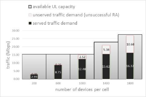
Figure 1: : At low to moderate device counts, minimal to negligible levels of collisions occur on the RA radio resources. However, mobile networks are already past this phase, i.e. the number of devices in a small cell is rapidly growing beyond 1000 [3].

The most straightforward proposition to alleviate RA congestion is to simply allocate additional radio resources for PRACH. This option obviously reduces the available resources for scheduling uplink data traffic. Moreover, allocating spectrally adjacent blocks for RA increases computational complexity at the BS side due to parallelized processing [4]. As such, it is not an appealing solution for the vendors. Another obvious proposition is to densify BS deployments as a mean to reduce congestion. Nonetheless, densification makes sense to mobile network operators only up to a certain limit. Beyond that, it ceases to offer either economic benefit [5] or performance improvement [6]. From the economic perspective, right-of-way and site acquisition costs may become major challenges. From the performance perspective, there is a critical density after which the coverage probability and rate degrade with BS density due to the overwhelming inter-cell interference. Another drawback for network densification is the increased handover rate for mobile users which consumes physical resources and incurs a delay [7, 8].

To this end, a distributed self-organized RA procedure is better positioned to accommodate this tremendous uplink demand in the future cellular networks. Indeed, standards for Long Term Evolution (LTE) have identified self-organization as a vital requirement for future networks [9]. The self-organized random access can response to actual network variations in near-real-time. Moreover, the self-organization random access is less costly since it entails the use of significantly less resource allocation complexity and administrative overhead.

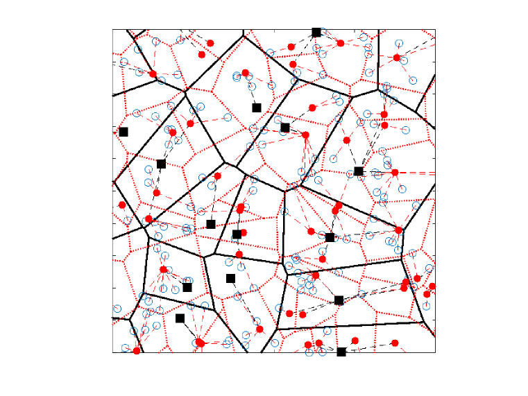
Figure 2: : Network realization for the system model for Devices-to-BS ratio $\alpha=16$ and cluster head selection probability $\delta=0.25$. The BSs are denoted by black squares, CHs are denoted by the red circles, and the CMs are denoted by blue circles. The Voronoi cell of the BSs are denoted by the solid black lines while the Voronoi cell of the CHs are denoted by the dotted red lines. The black dashed lines denote the associations of the CHs to the BSs while the red dashed line denote the associations of the CMs to the CHs. In this model, uplink and downlink interfaces can be decoupled, i.e., downlink traffic and signaling can be transmitted directly by the BS to the CMs.

I-A Prior Work

Device-to-device (D2D) relaying has been classically exploited within LTE networks, i.e., in-band D2D, mainly as a coverage improvement solution [10]. A corollary to coverage enhancements is indeed a boost in throughput or the spectrum efficiency through traffic offloading from cellular networks. In the stochastic geometry literature, different network architectures and systems were proposed to study and assess the spectrum sharing of in-band D2D communication [11, 12, 13, 14, 15, 16]. The authors in [17] analyze out-band D2D for uniform and k-closest content availability in terms of the coverage probability and the area spectral efficiency. Moreover, [18] studies the economic aspect of downlink traffic offloading via D2D for in-band and out-band operating modes. Furthermore, [19] develops an approach to model single- and multi-cluster wireless networks and study the coverage probability for closest-selection and uniform-selection strategies. It is worth to highlight that the model in [19] is suitable for downlink cellular networks or ad hoc networks. However, the idea of aggregating the uplink generated traffic within a cluster using out-band D2D communication in the presence of the cellular networks was investigated in [20, 21, 22]. The authors of [20] provide analytical expressions for the throughput and power consumption for a point-to-point scenario. In [21] the authors studied the latency-power trade-off of aggregating traffic on D2D links, where they showed that the transmit power can be reduced but at the expense of higher latency. Furthermore, [22] defines a protocol stack for the D2D communication in cellular networks, and uses system-level simulation to show the throughput improvement. However, none of the proposed protocols state the criterion and/or the effective scenarios to activate the D2D communication [10]. Most notably, D2D relaying literature rarely touches upon its advents relaying scheduling request to relieve RA congestion over the PRACH. While it may be quite intuitive, but a proper quantification of such an advantage is still missing out from literature.

I-B Contributions

This paper presents an out-band D2D relaying setup (e.g., WiFi Direct [22]) that can be exploited to boost the RA performance and LTE network capacity as well in dense networks. Within the context of this paper, the D2D paradigm refers to the situation where a number of devices cluster themselves together through an out-band link and assign a cluster head (CH) as depicted in Fig. 2. Uplink scheduling requests from cluster members (CM)s are forwarded to the assigned CH over unlicensed spectrum. The CH aggregates the requests from the CMs into larger ensembles and transmits one RA request per ensemble over the LTE interface. The BS process the RA request from the CHs and sends the uplink resources scheduling to the CMs directly through the downlink signaling. Without any doubt, such clustering relaxes the congestion over the LTE RA resources since the number of LTE RA requests is reduced, and hence, reduces the latency for resource allocation over the LTE interface. The problem is not trivial though. One has to consider whether the average access delay perceived by a device is actually enhanced by virtue of D2D clustering or not. This has to be evaluated in light of intra- and inter-cell interference. Indeed, this is the crux of the study carried out in this paper. The contribution of this work can be summarized as follows:

1. The paper proposes a self-organized D2D clustering in which each CH acts as a virtual Access Point (AP) over an LTE connection to boost the RA performance.

2. The paper considers two CH assignment mechanisms:

   • Random-Based Clustering (RBC) in which each device is assigned randomly with probability ($\delta$) to be a CH.

   • Channel-Gain-Based Clustering (CGBC) in which only the devices with channel gain greater than a threshold ($\tau$) are assigned to be CHs.

3. We present analytical expressions, based on stochastic geometry which takes into account the spatial intra and inter-cell/cluster interference sources to assess the transmissions success probabilities. Consequently, we quantify the average uplink scheduling delay for the D2D clustering.

4. The proposed self-organized D2D clustering scheme is benchmarked by the conventional RA procedure where all the devices have to send RA request to the BS over the LTE interface.

5. We quantify the critical device density beyond which the self-organized D2D clustering, for relaying uplink scheduling requests, offers performance gains (i.e., reduction in channel access delay).

6. For the range of device densities where D2D is feasible we answer the following crucial question: How to activate the D2D relaying and how should the CH be assigned? i.e., what are the suitable design parameters for these setups?

The results show that for the RBC and low device intensity is actually better to follow the conventional RA procedure. However, the self-organized D2D relaying scheme starts to pay off as the intensity grows. On the other hand, when the channel gains are considered in the CGBC scheme, D2D clustering provides higher delay reduction. Moreover, there is an optimal CH selection probability ($\delta$) or a channel gain threshold ($\tau$) that minimizes the average delay for every device intensity.

I-C Notation & Organization

Throughout the paper, we use the math italic font for scalars, e.g., $x$. We use the calligraphic font, e.g., $\mathcal{X}$ to represent a random variable (RV) while the math typewriter font, e.g., $\mathtt{x}$ is used to represent its instantiation. Moreover, $\mathbb{E}_{\mathcal{X}}\{\cdot\}$, $F_{\mathcal{X}}\left(\cdot\right)$, $\bar{F}_{\mathcal{X}}\left(\cdot\right)$, and $\mathscr{L}_{\mathcal{X}}\left(\cdot\right)$ denote, respectively, the expectation, the cumulative distribution function (CDF), the complementary cumulative distribution function (CCDF), and the Laplace Transform (LT) of the PDF of the random variable $\mathcal{X}$. We use $\mathbb{P}\{\cdot\}$ to denote the probability. $\mathbbm{1}_{\{\cdot\}}$ is the indicator function which has value of one if the statement $\{\cdot\}$ is true and zero otherwise. $\Gamma(\cdot)$ indicates the Gamma function and ${}_{2}F_{1}(.)$ is the Gaussian hypergeometric function. The imaginary unit is denoted by $j=\sqrt{-1}$ and imaginary component of a complex number is denoted as $\text{Im}\{.\}$. Lastly, $y^{*}$ denotes the optimal value of $y$.

The rest of the paper is organized as follows. Section II points out a high-level protocol description for the D2D clustering scheme. Section III models the physical layer attributes of the communication system and highlights the performance metrics. Section IV characterizes the D2D clustering protocols, while Section V provides the numerical results and insights. Section VI sheds light on some implementation obstacles and pertinent remedies and recommendations. Finally, Section VII summarizes and concludes the paper.

II Overiew of the Protocol

The goal of this section is not to define an exhaustive protocol stack for self-organized D2D clustering within LTE networks as in [22]. Rather, the aim is to point out a high-level description that helps to digest the presented scheme. The self-organized D2D clustering process can be summarized as follows:

1. D2D Clustering Initiation Order: the BS broadcasting this order along with the chosen value of the CH selection probability ($\delta$) over the downlink signaling.

2. CH Selection: for a given target fraction (i.e., $\delta$) of devices that are required to act as CHs, the clustering for each scheme is performed as follows:

   • for the RBC scheme, each device has a probability $\delta$ to be a CH. The selection can be done in a distributed manner, i.e., without the control of the BS. This can be done via a generating a random number $\mathtt{v}\in[0,1]$, and hence, the device becomes a CH if $\mathtt{v}\leq\delta$.

   • for the CGBC scheme, each device has to estimate its channel over the LTE interface and the device becomes a CH if the channel gain is greater than $\tau$, where $\tau$ is identified such that the fraction $\delta$ of devices are selected as CHs. Let $\mathtt{h}$ be the channel gain, then $\tau$ is identified through the inverse of the CCDF of $\mathtt{h}$ as $\tau=\bar{F}_{\mathtt{h}}^{-1}(\delta)=-\ln(\delta)$. Therefore, the selection can be done in a distributed manner as well.

3. CH Announcement: Once the CHs are identified each CH selects a frequency channel in the D2D spectrum and broadcasts its D2D-Identification (D2D-ID) to declare itself as a CH.

4. Cluster Formation: each CM scans the D2D channels searching for CHs broadcast messages. The CMs associate themselves to their nearest CH, by measuring the received signal strength (RSS) and selecting CH with the highest RSS. Through the association phase, the CMs send their D2D-ID along with their LTE-ID, e.g., SAE-Temporary Mobile Subscriber Identity (S-TMSI).

5. Cluster Registration at BS: each CH sends the D2D-LTE-ID association table to its serving BS via uplink LTE channel. Such a table is vital for the uplink resources scheduling so that the BS transmits the downlink signaling directly to the CMs.

Upon the D2D cluster formation, the CMs relay their uplink scheduling requests via the CH. The CH in turn, stamps the requests by the D2D-ID of the CMs, then aggregates all the RA requests from the CMs with its own request into a larger ensemble, and transmits one scheduling request via RA on the shared LTE PRACH for each ensemble.

III System Modeling & Assumptions

After describing the clustering process from a protocol point of view, this section portrays the modeling attributes of the proposed self-organized clustering schemes from a physical layer point of view.

III-A Spatial & Physical Layer Parameters

A two-tier cellular network is considered, namely the out-band D2D and LTE networks. Due to the disjoint spectrum allocation, the interference interactions on each network are decoupled. Since the cellular networks topologies from one location to another tend to be random, stochastic geometry is utilized to model the spatial distribution of the BSs as a point processes [24, 25, 26]. In this regards, the Poisson point process (PPP) is widely accepted and utilized due to its simplicity and practical relevance [26, 27, 28, 25]. Therefore, we assume that the BSs and the devices are spatially distributed according to two independent homogeneous PPPs with densities $\lambda$ and $\mu$, respectively. A power-law path-loss model is considered where the signal power decays at a rate of $r^{-\eta}$ with the propagation distance $r$, where $\eta>2$ is the path-loss exponent. In addition to the path-loss attenuation, Rayleigh block fading is assumed within a multi-path environment, in which all the channel power gains ($\mathtt{h}$) are assumed to be independent of each other and are identically and exponentially distributed with unity power gain.

III-B Random Access over the LTE Network

Each CH should go through the RA process over the PRACH to request uplink channel access from the BS [4]. The RA process is uncoordinated and all devices can mutually interfere with one another, which may lead to intra-cell interference in addition to the inter-cell interference. Only the CHs are eligible to request uplink resources over the LTE interface (i.e., PRACH) from the nearest BS. To request an uplink channel access, each CH randomly and independently transmits its RA request on one of the available prime-length orthogonal Zadoff-Chu (ZC) codes defined by the LTE PRACH preamble [4].

During the RA, each CH uses full path-loss inversion power control with target power level $\rho_{\text{L}}$ [4]. Therefore, the RA transmit power is expressed by $\mathcal{P}_{\text{{\rm RA}}}=\rho_{\text{L}}\mathcal{R}_{\text{L}}^{\eta}$, where $\mathcal{R}_{\text{L}}$ is the distance between the CH and its geographically closest BS. That is, the CH controls its transmit power such that the average signal power received at its serving BS is equal to $\rho_{\text{L}}$. The target power level $\rho_{\text{L}}$ is assumed to be conveyed on downlink signaling channels by the BS. It is assumed that the BSs are dense enough such that each of the CHs can invert its path-loss towards the closest BS almost surely, and hence the maximum transmit power of the IoT devices is not a binding constraint for packet transmission. Extension to fractional power control and/or adding a maximum power constraint can be done by following the methodologies in [29] and [30]. An RA transmission is assumed to be decodable if the signal to interference and noise ratio (SINR), denoted by $\Upsilon_{\text{{\rm RA}}}$, is greater than a certain threshold $\theta_{\text{{\rm RA}}}$.

III-C D2D Clustering Over an Unlicensed Spectrum

The clustering process is initiated by the BS where the clustering criterion, i.e., RBC or CGBC, is dictated by the BS. Each CM associates with its nearest CH through a single-hop link and relays the uplink scheduling requests via that link as shown in Fig. 2. CMs are assumed to employ full path-loss power control with target power level $\rho_{\text{C}}$. Therefore, the transmit power is given by $\mathcal{P}_{\text{D}}=\rho_{\text{C}}\mathcal{R}_{\text{C}}^{\eta}$, where $\mathcal{R}_{\text{C}}$ is the distance between the CM and its geographically closest CH. The target power level $\rho_{\text{c}}$ is assumed to be conveyed along with the D2D-ID of the CH in step 3 in Section II.

Each CH randomly and independently selects one of the $k$ available channels dedicated for D2D communications within the unlicensed spectrum. Moreover, transmission from CMs over the D2D interface is assumed to be managed by the CH via a time division multiple access (TDMA) schedule. Hence, intra-cluster interference is prohibited and only inter-cluster interference exists. Obviously, this comes at the expense of access delay that grows with the size of the cluster. For a correct transmission at the D2D link, an SINR capture model is adopted such that a transmission can be decoded if the SINR, denoted by $\Upsilon_{\text{C}}$, is greater than a certain threshold $\theta_{\text{C}}$.

IV Performance Analysis

Latency, or channel access delay to be more precise, is very important for several 5G application (e.g., tactile internet [31, 32]). It also has been a key aspect in the design objectives of cellular systems. Therefore, the channel access (i.e., resource allocation) delay is the primary metric used in this study to evaluate the gain of the self-organized D2D clustering scheme in reducing congestion over RA resources. Before delving into the analysis, we state the following important approximations that will be utilized in this paper.

Approximation 1.

The spatial correlations between proximate devices, in terms of transmission power, can be ignored.

Remark 1.

It is well known that the sizes of adjacent Voronoi cells are correlated. Such correlation affects the number of devices, as well as, the service distance realizations in adjacent Voronoi cells. Consequently, the transmission powers at adjacent cells are correlated. Accounting for such spatial correlation would impede the model tractability. Hence, we follow the common approach in the literature and ignore such spatial correlations when characterizing the aggregate interference [30, 33, 34, 35, 36, 37, 29, 38]. However, all spatial correlations are intrinsically accounted for in the Monte Carlo simulations that are used to validate our model in Section V.

Approximation 2.

For the D2D transmission, the point processes of inter-cluster interfering CMs seen at the test CH is modeled by a non-homogenous PPP.

Remark 2.

Despite that a PPP is used to model the complete set of CMs, the subset of scheduled CMs for the TDMA transmission is not a PPP. The constraint of scheduling one CM per Voronoi cell of the cluster leads to a Voronoi-perturbed point process for the set of mutually interfering CMs. Approximation 2 is commonly used in the literature to maintain tractability [30, 34, 36, 37, 29, 35, 38].

Approximation 3.

The transmission success probabilities of all devices in the network are assumed to have a negligible temporal correlation.

Remark 3.

The full path loss inversion makes the received signal power at the serving BSs/CHs independent from the service distance (i.e., the distance between the device and the serving BS/CH). Hence, the different realizations of the service distance across the devices do not affect the SINR. Furthermore, the random channel selection randomizes the set of interfering devices over different time slots, which decorrelate the interference across time. Hence, all devices in the network tend to have a negligible temporal correlation for the transmission success probabilities as shown in [33, 34, 35].

It is worth mentioning that Approximations 1-3 are mandatory for tractability, regularly used in the literature, and are validated in Section V via independent Monte-Carlo simulations. Based on these approximations, the D2D cluster size, the RA success probability, D2D success probability, and the channel access delay are presented in, respectively, Section IV-A, Section IV-B, Section IV-C, and Section IV-D. For a quick reference, the notation used in this paper is summarized in Table I.

Notation	Description
$\mu$; $\lambda$; $\alpha$	device density; BS density; devices-to-BS ratio
$\delta$; $\tau$	CH selection probability; channel gain threshold for CGBC
$\theta_{\text{{\rm RA}}}$	Detection threshold for successful RA
$\theta_{\text{C}}$	Detection threshold for successful D2D transmission
$\rho_{\text{L}}$; $\rho_{\text{c}}$	Power control parameter for RA; Power control parameter for D2D
$P_{\text{{\rm RA}}}$; $P_{\text{C}}$	RA success probability; D2D transmission success probability
${n_{Z}}$	number of ZC codes dectitated for random access
$k$	number of frequencies available for D2D transmission
$\eta$; $\sigma^{2}$	path-loss exponent; noise power

TABLE I: : Summary of Notation

IV-A D2D Cluster Size

Since the adopted clustering mechanisms are independent among all the devices, and by exploiting the independent thinning property of the PPP [39], the CHs constitute a PPP with intensity $\delta\mu$ [39]. Similarly, the CMs constitute a PPP with intensity $(1-\delta)\mu$. Moreover, due to the nearest CH association, the footprint of each CH can be expressed by a Voronoi cell with size and shape depending on the locations of its neighboring CHs as depicted in Fig. 2. Therefore, the number of CMs associated to each CH is random. Let $\mathcal{N}$ denote the number of CMs served by a generic CH, following [40], the probability mass function of $\mathcal{N}$ is given by:

$$\mathbb{P}\{\mathcal{N}=\mathtt{n}\}\approx\frac{\Gamma(\mathtt{n}+c)}{\Gamma(\mathtt{n}+1)\Gamma(c)}\frac{((1-\delta)\;\mu)^{\mathtt{n}}(\delta\;\mu c)^{c}}{((1-\delta)\;\mu+\delta\;\mu c)^{\mathtt{n}+c}},$$ (1)

where $c=3.575$ is a constant related to approximate the PDF of the PPP Voronoi cell area in $\mathbb{R}^{2}$. Let $\tilde{\delta}=(1-\delta)/\delta$, then (1) can be rewritten as:

$$\mathbb{P}\{\mathcal{N}=\mathtt{n}\}\approx\frac{\Gamma(\mathtt{n}+c)}{\Gamma(\mathtt{n}+1)\Gamma(c)}\left(\frac{\tilde{\delta}}{\tilde{\delta}+c}\right)^{\mathtt{n}}\left(\frac{c}{\tilde{\delta}+c}\right)^{c}.$$ (2)

It is worth noting that the D2D cluster size depends only on the CH selection probability ($\delta$) and is independent of the intensity of the devices $\mu$. As such, $\delta$ is a key performance factor that the protocol designers can use to optimize the delay. From (2), it can be shown that average cluster size $\mathbb{E}\left[\mathcal{N}\right]=\tilde{\delta}$.

$$\!F_{\mathcal{I}}\left(x\right)= \frac{1}{2}\!-\!\frac{1}{\pi}\!\!\int\limits_{0}^{\infty}\!\frac{1}{t}\text{Im}\left\{\exp\left\{-j\;t\;x\right\}{\exp\left\{\!\!\ \!-\!2\;\delta\;\alpha\;\rho^{2/\eta}_{\text{L}}\!\!\!\int\limits_{\rho_{\text{L}}^{\frac{-1}{\eta}}}^{\infty}\!\!\!\left(\!1\!-\!\frac{\exp\{j\;\tau\;t\;z^{-\eta}\}}{-j\;t\;z^{-\eta}+1}\!\right)z\;dz\right\}}{\left(1+\frac{\delta\;\alpha((1-j\;t\;\rho_{\text{L}})-\exp\{j\tau\;t\;\rho_{\text{L}}\})}{(1-j\;t\;\rho_{\text{L}})c}\right)^{-c}}\right\}dt.$$ (9)

IV-B RA Success Probability

Let $P_{\text{{\rm RA}}}=\mathbb{P}\left\{\Upsilon_{\text{{\rm RA}}}\!>\theta_{\text{{\rm RA}}}\right\}$ denote the probability that the CH’s RA attempt over the LTE interference is successful. As such, the SINR for the RA ($\Upsilon_{\text{{\rm RA}}}$) can be computed as follows:

$$\Upsilon_{\text{{\rm RA}}} =\frac{\rho_{\text{L}}\;\mathtt{h}_{\circ}}{{\sigma^{2}+\underset{m\in\tilde{{\Phi}}}{\sum}\mathtt{P}_{\text{{\rm RA}}m}\ \mathtt{h}_{m}\ \mathtt{R}_{m}\!^{-\eta}}},$$ (3)

where $\mathtt{h}_{\circ}$ represents the LTE channel gain between the test CH and its associated BS. $\sigma^{2}$ denotes the noise power and $\eta$ denotes the path-loss exponent. The set $\tilde{\Phi}$ contains all the interfering CHs that are simultaneously performing RA over the same ZC code, which may contain intra-cell and inter-cell interferes due to the uncoordinated nature of the RA. $\mathtt{P}_{\text{{\rm RA}}m},\ \mathtt{h}_{m},\ \text{and}\ \mathtt{R}_{m}$ represent, respectively, the transmit power, the channel gain, and the distance between the interfering CHs and the associated BS of the test CH. Due to the uncoordinated nature of the RA, there are two possible sources of interferences, namely the intra-cell interference and the inter-cell interference. Using stochastic geometry, we characterize the intra-cell and inter-cell interference on a test device via the LT of their probability density functions (PDFs). Then, the obtained LTs are used to derive the RA success probability, which is characterized in terms of CH selection probability ($\delta$) and the device-to-BS ratio ($\alpha$), i.e., $\alpha=\mu/\lambda$ .

From the independent thinning property of the PPP [39], the CHs interfering on the same ZC code constitute a PPP with intensity $\frac{\delta\;\mu}{{n_{Z}}}$, where $n_{Z}$ is the number of available ZC codes. Consequently, the average number of CHs that may use the same ZC code per BS is given by ${\tilde{\alpha}}=\frac{\delta\;\mu}{\lambda\;n_{Z}}$. By the PPP assumption, the number and locations of the points in disjoint areas are independent. Consequently, the intra-cell and inter-cell interference are independent. Exploiting this fact, the success probability for each of the clustering schemes is given in the sequel.

IV-B1 RBC Scheme

The RA success probability for the RBC can be expressed as

$$P_{\text{{\rm RA}}}= \mathbb{P}\left\{\frac{\rho_{\text{L}}\;\mathtt{h}_{\circ}}{\sigma^{2}+\mathcal{I}_{\text{In}}+\mathcal{I}_{\text{Out}}}>\theta_{\text{{\rm RA}}}\right\}$$

$$\overset{(a)}{=} \exp\left\{-\frac{\sigma^{2}\theta_{\text{{\rm RA}}}}{\rho_{\text{L}}}\right\}\mathscr{L}_{\mathcal{I}_{\text{In}}}\left(\frac{\theta_{\text{{\rm RA}}}}{\rho_{\text{L}}}\right)\mathscr{L}_{\mathcal{I}_{\text{Out}}}\left(\frac{\theta_{\text{{\rm RA}}}}{\rho_{\text{L}}}\right){,}$$ (4)

where ${\mathcal{I}_{\text{In}}}$ is the intra-cell interference and ${\mathcal{I}_{\text{Out}}}$ is the inter-cell interference. Note that $(a)$ in (4) follows from the exponential distribution of $\mathtt{h}_{\circ}$ [41]. The RA access success probability in (4) is characterized with the following theorem.

Theorem 1.

The RA access success probability in a PPP network and Random-Based Clustering where each CH employs full path-loss inversion power control is given by:

$${P_{\text{{\rm RA}}}} \;{\approx}\;\frac{\exp\left\{-\frac{\sigma^{2}\theta_{\text{{\rm RA}}}}{\rho_{\text{L}}}-\frac{2\;\delta\;\alpha\;\theta_{\text{{\rm RA}}}}{n_{Z}(\eta-2)}\;{}_{2}F_{1}\left(1,1-\frac{2}{\eta},2-\frac{2}{\eta},-\theta_{\text{{\rm RA}}}\right)\right\}}{\left(1+\frac{\delta\;\alpha\;\theta_{\text{{\rm RA}}}}{n_{Z}(1+\theta_{\text{{\rm RA}}})c}\right)^{c}},$$ (5)

where $c=3.575$ is a constant related to the approximate PDF of the PPP Voronoi cell area in $\mathbb{R}^{2}$.

Proof.

Similar to [35, Lemma 1], where 5 is not exact due to ignoring the spatial correlations among the transmission powers of the CHs as mentioned earlier in Approximation 1. ∎

For the special case of $\eta=4$, which is a typical path loss exponent for urban outdoor environment, (5) reduces to:

$${P_{\text{{\rm RA}}}}\;{\approx}\;\frac{\exp\left\{-\frac{\sigma^{2}\theta_{\text{{\rm RA}}}}{\rho_{\text{L}}}-\frac{\delta\alpha}{n_{Z}}\sqrt{\theta_{\text{{\rm RA}}}}\arctan\left({\sqrt{\theta_{\text{{\rm RA}}}}}\right)\right\}}{\left(1+\frac{\delta\alpha\theta_{\text{{\rm RA}}}}{n_{Z}(1+\theta_{\text{{\rm RA}}})c}\right)^{c}}.$$ (6)

The expression in (6) gives the RA success probability in terms of the elementary arctan function instead of the computationally complex Gaussian hypergeometric function.

IV-B2 CGBC Scheme

The RA success probability for the CGBC scheme can be expressed as:

$$P_{\text{{\rm RA}}}= \mathbb{P}\left\{\frac{\rho_{\text{L}}\;\mathtt{h}_{\circ}}{\sigma^{2}+\mathcal{I}_{\text{In}\mid\mathtt{h}>\tau}+\mathcal{I}_{\text{Out}\mid\mathtt{h}>\tau}}>\theta_{\text{{\rm RA}}}\mid\mathtt{h}>\tau\right\}$$

$$\overset{(b)}{=} \begin{cases}\exp\left\{-\frac{\sigma^{2}\theta_{\text{{\rm RA}}}}{\rho_{\text{L}}}+\tau\right\}\mathscr{L}_{\mathcal{I}_{\text{In}}\mid\mathtt{h}>\tau}\left(\frac{\theta_{\text{{\rm RA}}}}{\rho_{\text{L}}}\right)\\ \quad\quad\quad\quad\quad\quad\times\mathscr{L}_{\mathcal{I}_{\text{Out}}\mid\mathtt{h}>\tau}\left(\frac{\theta_{\text{{\rm RA}}}}{\rho_{\text{L}}}\right),&\frac{\theta_{\text{{\rm RA}}}(\sigma^{2}+\mathcal{I})}{\rho_{\text{L}}}>\tau\\ 1,&\text{otherwise{,}}\end{cases}$$ (7)

where ${\mathcal{I}_{\text{In}\mid\mathtt{h}>\tau}}$ is the intra-cell interference given that the interfering CHs have channel gain greater than $\tau$, ${\mathcal{I}_{\text{Out}\mid\mathtt{h}>\tau}}$ is the inter-cell interference given that the interfering CHs have channel gain greater than $\tau$, and $\mathcal{I}$ is the total interference. Note that $(b)$ in (IV-B2) follows from the exponential distribution of $\mathtt{h}_{\circ}$ [41]. The RA access success probability in (IV-B2) is characterized by the following theorem.

Theorem 2.

The RA access success probability in a PPP network and Channel-Gain-Based Clustering where each CH employs full path-loss inversion power control is given by

$${P_{\text{{\rm RA}}}}\;{\approx}\; \frac{\exp\left\{\!\!\!-\frac{\sigma^{2}\theta_{\text{{\rm RA}}}}{\rho_{\text{L}}}\!+\!\tau\!-\!2\;\delta\;\alpha\;\theta^{2/\eta}_{\text{{\rm RA}}}\!\!\!\int\limits_{\theta_{\text{{\rm RA}}}^{\frac{-1}{\eta}}}^{\infty}\!\!\!\left(\!1\!-\!\frac{\exp\{\!-\tau y^{-\eta}\!\}}{y^{-\eta}+1}\!\right)y\;dy\right\}}{\left(1+\frac{\delta\;\alpha((1+\theta_{\text{{\rm RA}}})-\exp\{-\tau\theta_{\text{{\rm RA}}}\})}{(1+\theta_{\text{{\rm RA}}})c}\right)^{c}}$$

$$\times \bar{F}_{\mathcal{I}}\left(\frac{\tau\;\rho_{\text{L}}}{\theta_{\text{{\rm RA}}}}-\sigma^{2}\right)+F_{\mathcal{I}}\left(\frac{\tau\;\rho_{\text{L}}}{\theta_{\text{{\rm RA}}}}-\sigma^{2}\right),$$ (8)

where $c=3.575$ is a constant related to the approximate PDF of the PPP Voronoi cell area in $\mathbb{R}^{2}$ and $F_{\mathcal{I}}\left(x\right)$ is the CDF of the aggregated interference which has the form of (9) in the bottom of this page.

Proof.

See Appendix -A, where 2 is not exact due to ignoring the spatial correlations among the transmission powers of the CHs as mentioned earlier in Approximation 1. ∎

IV-C D2D Transmission Success Probability

On the D2D links, each CH aggregates the uplink scheduling requests originated from its associated CMs TDMA scheduling. Hence, inter-cluster interference and noise are the only two channel impairment for D2D transmission. Therefore, the transmission SINR for the D2D relaying can be computed as follows:

$$\Upsilon_{\text{C}} =\frac{\rho_{\text{C}}\;\mathtt{h}_{\ast}}{{\sigma^{2}+\underset{i\in{{\Phi}}}{\sum}\mathtt{P}_{\text{D}i}\ \mathtt{h}_{i}\ \mathtt{R}_{i}\!^{-\eta}}},$$ (10)

where $\mathtt{h}_{\ast}$ represents the D2D channel gain between the test CM and its associated CH. The set $\Phi$ contains all the interfering CMs that transmit simultaneously over the same frequency, which are one CM per cluster due to the TDMA scheduling. $\mathtt{P}_{\text{D}i},\ \mathtt{h}_{i},$ and $\mathtt{R}_{i}$ represent the transmit power, the channel gain, and the distance between the interfering CMs and the associated CH of the test CM. To characterize $\Upsilon_{\text{C}}$, we follow a similar methodology described for $\Upsilon_{\text{RA}}$, while accounting for the fact that each CH has a single active CM to serve at a given time instant. Hence, the intensity of interfering CMs on each channel is equal to the intensity of the CHs that selected the same frequency, i.e., intensity of interfering CMs is $\frac{\delta\;\mu}{k}$, where $k$ is the number of frequencies available for D2D transmission. Consequently, the D2D success probability $P_{\text{C}}=\mathbb{P}\left\{\Upsilon_{\text{C}}\!>\theta_{\text{C}}\right\}$ is characterized by the following theorem.

Theorem 3.

The probability of successful uplink scheduling request over a PPP D2D link where each CM employs full path-loss inversion power control, can be expressed as

$${P_{\text{C}}} \;{\approx}\;\exp\left\{-\frac{\sigma^{2}\theta_{\text{C}}}{\rho_{\text{C}}}-\frac{2\theta_{\text{C}}}{k(\eta-2)}\;{}_{2}F_{1}\left(1,1-\frac{2}{\eta},2-\frac{2}{\eta},-\theta_{\text{C}}\right)\right\}.$$ (11)

Proof.

Similar to [36, Theorem 1], where (11) is not exact due to ignoring the spatial correlations among the transmission powers of the CMs as mentioned earlier in Approximation 1 and due to approximating the inter-cluster interfering CMs with a PPP as mentioned in Approximation 2. ∎

For the special case of $\eta=4$, (11) reduces to:

$${P_{C}}\;{\approx}\;\exp\left\{-\frac{\sigma^{2}\theta_{\text{C}}}{\rho_{\text{C}}}-\frac{\sqrt{\theta_{\text{C}}}}{k}\arctan\left({\sqrt{\theta_{\text{C}}}}\right)\right\}.$$ (12)

It is worthwhile to mention that the approximations in (5), (2), and (11) are mandatory for tractability and are common in stochastic geometry analysis for uplink systems [29, 30, 37].

IV-D Channel Access Delay ($D$)

The channel access delay ($D$) is defined as the average number of time slots required by a device before the uplink transmission is successfully scheduled. In the depicted communication system, where the CMs sends their requests to the CH via a TDMA schedule, $D$ is given by

$$D {\approx}\frac{1}{P_{\text{{\rm RA}}}}+\frac{\mathbb{E}\left[\mathcal{N}\right]}{P_{\text{C}}},$$ (13)

which is derived by modeling the trials for both of the RA and the D2D transmissions by geometric random variables. In addition, the mean number of CMs associated to a CH ($\mathbb{E}\left[\mathcal{N}\right]$) is introduced here to take into account the TDMA scheduling. It is worth to highlight that (13) is not exact due to ignoring the negligible temporal correlation of the transmission success probabilities as mentioned in Approximation 3.

V Numerical Results

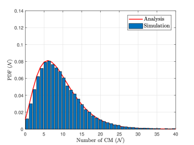
(a) $\mu=160$, $\delta=.1$

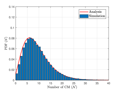
(b) $\mu=640$, $\delta=.1$

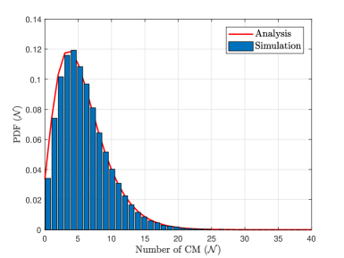
(c) $\mu=160$, $\delta=.15$

(d) $\mu=640$, $\delta=.15$

Figure 3: : The PDF of the number of CMs associated to a CH for for $\mu=160\text{ and }640$ UE/km² for different values of CH probability $\delta=.1$ and $.15$.

This section first validates the developed model via independent Monte Carlo simulations. Then, selected numerical results are presented to assess and compare the performance of the RBC and CGBC schemes. In each simulation run, the BSs and the devices are realized over a 100 km² area via independent PPPs and the collected statistics are taken for devices located within 1 km from the origin to avoid the edge effects. First, we examine the D2D cluster size in (2). Fig. 3 shows the PDF of the associated CMs for each CH for $\mu=160\text{ and }640$ UE/km² for different values of CH selection probability $\delta=0.1$ and $0.15$. Fig. 3 supports the remark given in Section IV-A about the independence of the PDF of $\mathcal{N}$ from the devices intensity. This can be explained as follows: The cluster’s geographical footprint is represented by a Voronoi cell whose average area is $\bar{d}=\frac{1}{\delta\mu}$. The average geographical footprint $\bar{d}$ of the cluster shrinks as more devices are elected as CHs. However, the intensity of CMs also increases such that the cluster size in terms of number of CMs stays constant. Fig. 3 also shows that as $\delta$ increases, the D2D cluster size becomes smaller, and hence, the PDF of $\mathcal{N}$ is pushed to have a smaller mean.

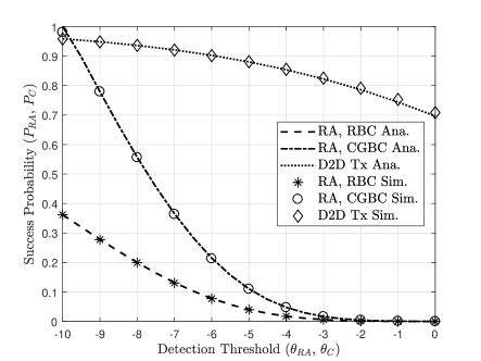
(a) $\alpha=16$ device/BS.

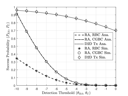
(b) $\alpha=64$ device/BS.

Figure 4: : The RA and D2D transmission success probability as a function of $\theta_{\text{{\rm RA}}}$ and $\theta_{\text{C}}$ for CH selection probability $\delta=0.35$.

Fig. 4 depicts the RA transmission success probabilities for RBC and CGBC schemes along with the D2D transmission success probability. The simulation parameters are as follows; $\mu=160$ and $640$ device/km², $\lambda=10$ BS/km², and equivalently, $\alpha=16$ and $64$ device/BS. CH selection probability $\delta=0.35$, $n_{z}$= 64 code per BS, $\rho_{\text{C}}=-80$ dBm, $\rho_{\text{RA}}=-100$ dBm, noise power $\sigma^{2}=-90$ dBm, number of frequencies available for D2D transmission $k=3$, and path-loss exponent $\eta=4$. It is important to note the close match between the analysis and simulation results which validates the developed mathematical framework and Approximations 1-2.

Notation	Description	Value
$\mu$	device densities	$160$ and $640$ devices/km2
$\lambda$	BS density	$10$ BS/km2
${n_{Z}}$	number of ZC codes dectitated for random access	$64$ code per BS
$\delta$	CH probability	$[.1,1]$
$\theta_{\text{C}}$	Detection threshold for successful D2D transmission	$-7$ dB
$\theta_{\text{{\rm RA}}}$	Detection threshold for successful RA	$-7$ dB
$\rho_{\text{c}}$	Power control parameter for D2D	$-80$ dBm
$\rho_{\text{L}}$	Power control parameter for RA	$-100$ dBm
$\sigma^{2}$	noise power	$-90$ dBm
$k$	number of frequencies available for D2D transmission	$3$
$\eta$	path-loss exponent	$4$

TABLE II: : Numerical Evaluation Parameters

At this point of the discussion, we look into the channel access delay as a key performance metric. The conventional RA procedure is used as a benchmark to evaluate the performance of the proposed D2D clustering procedure. It is worth mentioning that the conventional RA procedure is a special case of the RBC D2D clustering by setting $\delta=1$, also it is a special case of the CGBC D2D clustering by setting $\tau=0$. The parameters used in this section are summarized in Table II.

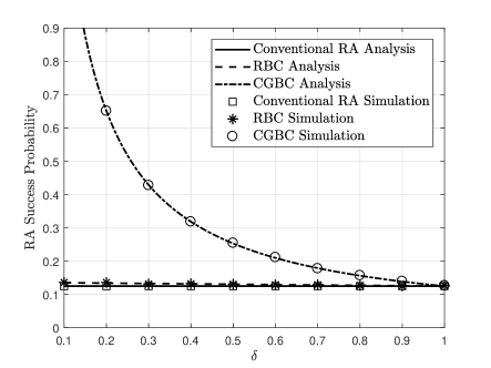
(a) $\alpha=16$ device/BS.

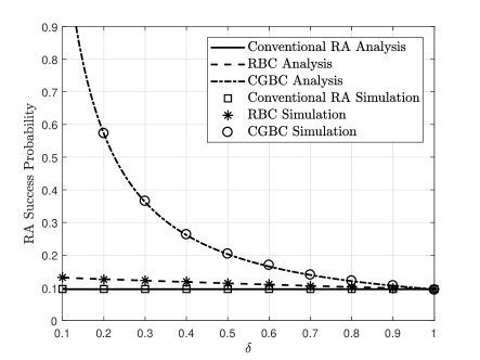
(b) $\alpha=64$ device/BS.

Figure 5: : The RA success probability as a function of CH selection probability $\delta$.

Fig. 5 and Fig. 6 show respectively the RA success probability and the delay as a function of $\delta$. As expected, Fig. 5 shows that the RA success probability for both the D2D clustering and the conventional cases decreases as $\alpha$ grows. And in turn, the delay increases as $\alpha$ increases. Also, Fig. 5 shows that as the CH selection probability $\delta$ increases the RA success probability for D2D clustering decreases. This is due to the fact that as $\delta$ increases, more CHs are eligible to perform an RA procedure over the LTE interface. Therefore, both of the inter-cell and intra-cell interference increases leading to lower RA success probability ($P_{\text{{\rm RA}}}$). Furthermore, the results show that CGBC D2D clustering offers the highest RA success probability.

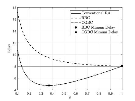
(a) $\alpha=16$ device/BS.

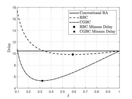
(b) $\alpha=64$ device/BS.

Figure 6: : The average delay needed for successful RA as a function of CH selection probability $\delta$.

For insightful conclusions, Fig. 5 and Fig. 6 should be considered jointly. While one case may be favorable from the RA success probability perspective, it may be invoking too much delay and an adverse impact on the average waiting time for a successful RA. Fig. 6 gives an interesting insight by comparing performance at two device densities. For RBC D2D clustering, the RA performance will not gain any benefit at low device densities. Regardless how aggressive $\delta$ is, the conventional case always offers lower channel access delay. From a mere RA perspective, it is simply just not worth it to use D2D clustering. However, the RBC D2D clustering starts to pay off at high intensities as shown in Fig.6. On the other hand, the CGBC offers an improvement over the conventional RA even for low device intensities as shown Fig. 6.

It is straightforward to notice the trade-off between the delay and the CH selection probability $\delta$ or equivalently $\tau$. Specifically, $\delta$ has a two-fold effect on the delay as can be inferred from Eq. (13). First, the larger the $\delta$ the more device are eligible to be CHs, and hence, the smaller cluster size in terms of the number of the associated CMs. Therefore, smaller number of CMs results in a shorter delay in the TDMA scheduled transmission. As such, the right-hand term of Eq. (13) decreases because the numerator ($\mathcal{N}$) decreases while the denominator ($P_{C}$) is not intact with the change of $\delta$. Second, it is worthy recalling however that larger $\delta$ means a larger number of CHs, which leads to degraded success probability of the RA over the LTE PRACH interface. In more precise terms, the first term of Eq. (13) increases as $\delta$ increases. To sum up, the first term of Eq. (13) is a negative monotone in $\delta$ while the second is positive monotone. Consequently, $\delta$ can be optimized to achieve a minimum delay. For example, employing RBC D2D clustering and at $\alpha=64$ device/BS with a value of ${\delta^{*}}=0.59$ minimizes the delay with a rate of $6\%$ when compared to the conventional RA case. On the other hand, for CGBC D2D clustering and at $\alpha=16$ device/BS with a value of ${\tau^{*}}=-0.025$ dB and a corresponding value of ${\delta^{*}}=0.37$ would minimize the delay at a reduction rate of $40\%$ when compared to the conventional RA case. While at $\alpha=64$ device/BS, ${\tau^{*}}=0.567$ dB with a corresponding value of ${\delta^{*}}=0.32$ would minimize the delay at a reduction rate of $49\%$.

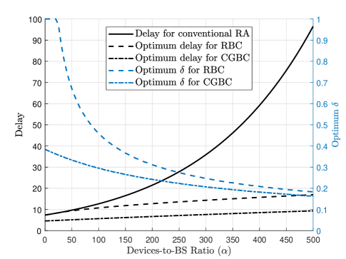
Figure 7: : Optimum delay and the corresponding values of ${\delta^{*}}$ as a function of the devices-to-BS ratio ($\alpha$).

Fig. 7 depicts the optimum delay and the corresponding value of the CM selection probability ($\delta$) for both RBC and CBGC clustering schemes. The result shows that the RBC starts to offer a reduction in the RA access delay when devices-to-BS ratio becomes larger than 50. However, the CBGC always offers an enhancement over the conventional RA. Another insightful observation from Fig. 7 is that as $\alpha$ increases, $\delta$ decreases. This behavior is mainly due to the fact that the RA congestion over the LTE interface is more critical when the devices intensity increases compared with the delay that stems from the TDMA transmission within the D2D cluster.

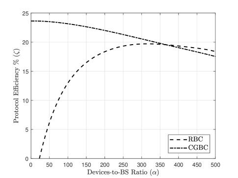
Figure 8: : Protocol efficiency for optimum delay reduction rate as a function of the devices-to-BS ratio ($\alpha$).

It should be mentioned, however, that the improved performance of the CGBC scheme comes at the cost of higher protocol overhead. That can be justified by the lower optimal CH selection probability, which leads to higher cluster population for the CGBC scheme, and in turn, larger signaling in the cluster formation process. As such, there is a need to quantify the protocol efficiency which can be defined by the delay reduction rate over the protocol overhead. We consider the average cluster size $\mathbb{E}\left[\mathcal{N}\right]$ as a measure for the protocol overhead. Therefore the protocol efficiency ($\zeta$) can be calculated as follows:

$$\zeta=\frac{D(\delta={\delta^{*}})-D(\delta=1)}{D(\delta=1)\mathbb{E}\;\left[\mathcal{N}\right]}\times 100\%,$$ (14)

where $D(\delta)$ is the delay in (13) as a function of the CH selection probability $(\delta)$.

Fig. 8 shows the protocol efficiency for the optimal delay in Fig. 7. The figure shows that even though the CGBC provides a lower delay, the protocol efficiency is lower when the devices intensity scales. Specifically, it is more rewarding in terms of protocol efficiency to follow the RBC scheme when the devices intensity goes beyond $370$ devices/BS.

VI Implementation, Issues, $\&$ remedies

The foreseen gain that Fig. 7 depicts can be best achieved through an automated self-optimization algorithm. Such an algorithm can be implemented through a back-end script at the network core whose goal is to estimate network parameters and calculate the optimum value of CHs selection probability ($\delta$) for RBC and CGBC schemes. The analytical results in Section IV show that the performance of the proposed D2D clustering schemes depends on three estimated parameters, namely, the intensity of BSs, the devices intensity, and the path-loss exponent. The intensity of BSs may be the easiest parameter to estimate as the number of BSs in a geographic area is available to the operators, then the intensity of BSs can be estimated accordingly. The devices intensity, on the other hand, can be estimated through event-triggered reporting for the association table. As such, the CH reports to the BS any change occurred to its associated CMs, then the BS, in turn, reports this change to the core network. The core network can estimate the current device intensity and then broadcast the optimum value of $\delta$ in a reclustering order. Moreover, for the CGBC scheme, the CHs are required to report to the BS if the estimated channel gain goes below the threshold $\tau$. In this case, the BS can broadcast a reclustering order to maintain the performance edge. Lastly, the path-loss exponent estimation can be done by a self-estimator that only requires collecting multiple Received Signal Strength (RSS) as in [42] which can be executed easily due to its independence. The pseudo code for the back-end self-optimization script is shown in Algorithm 1, where the optimization problems in (16) and (17) can be solved via a one-dimensional line search with an initial uncertainty range of $I_{\circ}\in(0,1]$. One of the algorithms that can be used to solve (16) and (17) is the golden-section search. The number of golden-section search iterations ($n$) that achieves an accuracy of ($\epsilon$) for the can be estimated by [43]

$$n\geq\log_{K}\frac{I_{\circ}}{\epsilon},$$ (15)

where $K=(1+\sqrt{5})/2$ is the golden ratio constant. For example, the golden-section search achieves an accuracy of $\epsilon=10^{-6}$ with $n=29$ iterations and only $30$ function evaluations. The brute-force method, on the other hand, requires $10^{\;6}$ function evaluations to find a $\delta^{*}$ with the same accuracy.

Algorithm 1 ​​: Pseudo code for the back-end self-optimization script.

1:Estimate $\lambda,\mu,\eta$.

2:Solve the optimization problem of $D$ in (13) for RBC scheme as:

$$\underset{\delta}{\text{minimize}} D_{\text{RBC}}=\frac{1}{P_{\text{{\rm RA}}}}+\frac{\tilde{\delta}}{P_{\text{C}}}.$$ (16)

subject to $$0<\delta\leq 1$$

where $P_{\text{{\rm RA}}}$ can be evaluated by (5).

3:Solve the optimization problem of $D$ in (13) for CGBC scheme as:

$$\underset{\delta}{\text{minimize}} D_{\text{CGBC}}=\frac{1}{P_{\text{{\rm RA}}}}+\frac{\tilde{\delta}}{P_{\text{C}}}.$$ (17)

subject to $$0<\delta\leq 1$$

where $P_{\text{{\rm RA}}}$ can be evaluated by (2), and $\tau=-\ln(\delta)$.

4:Compare $D_{\text{RBC}}$ and $D_{\text{CGBC}}$ and select the scheme that results in lower $D$.

5:Return the optimum $\delta$ and the selected scheme.

However, incentivizing and commercializing D2D clustering have been dwelling in a slightly stagnant state for some time due to some practical concerns. First, one of the major implementation challenges of the proposed scheme is that the CM may fall in a BS footprint different than the CH is associated to. Since the uplink resources are better granted to the devices by the closest BS, the core network is in the best position to process the uplink resource scheduling such that each device is granted uplink resources from the nearest BS. Second, the use of D2D clustering network to reroute uplink scheduling requests entails fairness issues regarding battery depletion rates of the CHs. Furthermore, the proposed D2D clustering entails low-layer modifications to the protocol stack something that needs to be taken into standardization meetings.

VII Conclusions

This paper introduces a self-organized D2D clustering scheme to relieve the congestion on the RA resources in massively loaded networks. Two D2D clustering schemes are studied, namely, RBC and CGBC. The results show that the RBC scheme offers no delay reduction at low device densities and hence it is preferable to follow the conventional access model. As the device intensity grows, the RBC starts to offer reduced delay and there is an optimal value of CHs selection probability ($\delta$) that minimizes the delay. To maintain the performance edge of the RBC, the BS has to revisit the clustering relationships whenever the intensity changes. On the other hand, the CGBC offers significant performance gains when compared to both the conventional and RBC schemes even for low device intensities. However, the gain edge comes at the cost of higher overhead due to the larger cluster size, and hence, larger signaling in the clustering process. As such the two schemes offer a trade-off between complexity and performance. To this end, a self-optimization algorithm to execute the D2D clustering is presented. We also highlight a few remedies and recommendations for practical implementation.

-A Proof of Theorem 2.

Note that the nearest BS association and the employed power control enforce the following two conditions; (i) the intra-cell interference from an interfering device is equal to $\rho_{\text{L}}$, and (ii) the inter-cell interference from any interfering device is strictly less than $\rho_{\text{L}}$. The aggregated inter-cell interference received at the BS is obtained as:

$$\mathcal{I}_{\text{out}\mid\mathtt{h}>\tau}=\sum\limits_{m\in\tilde{{\Phi}}}\mathbbm{1}_{{\{}\mathtt{P}_{\text{{\rm RA}}m}\mathtt{R}_{m}\!^{-\eta}<\rho_{\text{L}}\}}\mathtt{P}_{\text{{\rm RA}}m}\ \mathtt{h}_{m}\ \mathtt{R}_{m}\!^{-\eta}.$$ (18)

Approximating the set of interfering devices by a PPP with independent transmit powers, the Laplace Transform of (18) can be approximated as (-A).

$$\mathscr{L}_{\mathcal{I}_{\text{out}\mid\mathtt{h}>\tau}}(s)\approx\exp\Bigg{\{}-2\pi\;\delta\;\alpha\lambda\;\mathbb{E}_{\mathcal{P}_{\text{{\rm RA}}}}\left[\mathcal{P}_{\text{{\rm RA}}}^{\frac{2}{\eta}}\;\right]$$

$$\times\int\limits_{(\rho_{\text{L}})^{\frac{-1}{\eta}}}^{\infty}\left(1-\frac{\exp\{-\tau s\;y^{-\eta}\}}{s\;y^{-\eta}+1}\right)\;y\;dy\Bigg{\}}.$$ (19)

The LT is obtained by using the probability generating function (PGFL) of the PPP [39] and following [36], where the LT is obtained by substituting the value of $\mathbb{E}_{\mathcal{P}_{\text{{\rm RA}}}}\left[\mathcal{P}_{\text{{\rm RA}}}^{\frac{2}{\eta}}\right]$ from [Lemma 1,[36]]. The Intra-cell interference conditioned on the number of neighbors is given by:

$$\small\mathcal{I}_{\text{in}\mid\mathtt{h}>\tau,\mathtt{n}}=\displaystyle{\sum\limits_{i=1}^{\mathtt{n}}\rho_{\text{L}}\mathtt{h}_{i}}.\normalsize$$ (20)

The Laplace Transform of (20) is obtained as:

$$\small\mathscr{L}_{\mathcal{I}_{\text{in}\mid\mathtt{h}>\tau,\mathtt{n}}}(s) =\mathbb{E}[e^{-s\mathcal{I}_{\text{in}\mid\mathtt{h}>\tau,\mathtt{n}}}]=\frac{\exp\{-\mathtt{n}\tau s\rho_{\text{L}}\}}{(1+s\rho_{\text{L}})^{\mathtt{n}}}.\normalsize$$ (21)

The probability mass function of the number of neighbors $\mathcal{N}$ which is found in [40] as:

$$\mathbb{P}\{\mathcal{N}=\mathtt{n}\}\approx\frac{\Gamma(\mathtt{n}+c)}{\Gamma(\mathtt{n}+1)\Gamma(c)}\frac{\left(\frac{\delta\;\mu}{n_{Z}}\right)^{\mathtt{n}}(\lambda c)^{c}}{\left(\frac{\delta\;\mu}{n_{Z}}+\lambda c\right)^{\mathtt{n}+c}}.$$ (22)

Considering that there is only Inter-cell interference when the number of neighbors in the cell is 0, and both of inter-cell and intra-cell interference otherwise we can write equation (IV-B2) as (-A).

$${P_{\text{{\rm RA}}}} =\exp\left\{\!-\frac{\sigma^{2}\theta_{\text{{\rm RA}}}}{\rho_{\text{L}}}+\tau\right\}\mathscr{L}_{\mathcal{I}_{\text{out}\mid\mathtt{h}>\tau}}\left(\frac{\theta_{\text{{\rm RA}}}}{\rho_{\text{L}}}\right)$$

$$\quad\times\left[\mathbb{P}\left\{\mathcal{N}=0\right\}+\!{\sum\limits_{\mathtt{n}=1}^{\infty}\mathbb{P}\left\{\mathcal{N}=\mathtt{n}\right\}\times\mathscr{L}_{\mathcal{I}_{\text{in}\mid\mathtt{h}>\tau,\mathtt{n}}}\left(\frac{\theta_{\text{{\rm RA}}}}{\rho_{\text{L}}}\right)}\right].$$ (23)

To take into account the boundaries in (IV-B2), we use Gil-Pelaez theorem [44]. Therefore, the CDF of the aggregated interference $F_{\mathcal{I}}\left(x\right)$ can be calculated by:

$$F_{\mathcal{I}}\left(x\right)= \frac{1}{2}-\frac{1}{\pi}\int\limits_{0}^{\infty}\frac{1}{t}\text{Im}\left\{\exp\left\{-j\;t\;x\right\}\mathscr{L}_{\mathcal{I}}\left(-j\;t\right)\right\}dt,$$ (24)

where $\mathscr{L}_{\mathcal{I}}$ is the Laplace Transform of the aggregated interference which has the form of:

$$\mathscr{L}_{\mathcal{I}}(s)= \mathscr{L}_{\mathcal{I}_{\text{out}\mid\mathtt{h}>\tau}}\left(s\right)$$

$$\quad\times\left[\mathbb{P}\left\{\mathcal{N}=0\right\}+\!{\sum\limits_{\mathtt{n}=1}^{\infty}\mathbb{P}\left\{\mathcal{N}=\mathtt{n}\right\}\times\mathscr{L}_{\mathcal{I}_{\text{in}\mid\mathtt{h}>\tau,\mathtt{n}}}\left(s\right)}\right].$$ (25)

After Applying the total probability theorem (2) is obtained.

References

- [1] J. G. Andrews, S. Buzzi, W. Choi, S. V. Hanly, A. Lozano, A. C. K. Soong, and J. C. Zhang, “What will 5G be?” IEEE Journal on Selected Areas in Communications, vol. 32, no. 6, pp. 1065–1082, June 2014.
- [2] B. Romanous, N. Bitar, A. Imran, and H. Refai, “Network densification: Challenges and opportunities in enabling 5G,” in IEEE 20th International Workshop on Computer Aided Modelling and Design of Communication Links and Networks (CAMAD), 2015, pp. 129–134.
- [3] A. Bader, H. ElSawy, M. Gharbieh, M. S. Alouini, A. Adinoyi, and F. Alshaalan, “First mile challenges for large-scale IoT,” IEEE Communications Magazine, vol. 55, no. 3, pp. 138–144, March 2017.
- [4] S. Sesia, I. Toufik, and M. Baker, LTE: the UMTS long term evolution. Wiley Online Library, 2009.
- [5] J. Park, S. L. Kim, and J. Zander, “Asymptotic behavior of ultra-dense cellular networks and its economic impact,” in 2014 IEEE Global Communications Conference, Dec 2014, pp. 4941–4946.
- [6] A. AlAmmouri, J. G. Andrews, and F. Baccelli, “SINR and throughput of dense cellular networks with stretched exponential path loss,” IEEE Transactions on Wireless Communications, vol. 17, no. 2, pp. 1147–1160, Feb 2018.
- [7] R. Arshad, H. ElSawy, S. Sorour, T. Y. Al-Naffouri, and M. S. Alouini, “Velocity-aware handover management in two-tier cellular networks,” IEEE Transactions on Wireless Communications, vol. 16, no. 3, pp. 1851–1867, March 2017.
- [8] R. Arshad, H. Elsawy, S. Sorour, M. S. Alouini, and T. Y. Al-Naffouri, “Mobility-aware user association in uplink cellular networks,” IEEE Communications Letters, vol. 21, no. 11, pp. 2452–2455, Nov 2017.
- [9] O. G. Aliu, A. Imran, M. A. Imran, and B. Evans, “A survey of self organisation in future cellular networks,” IEEE Communications Surveys Tutorials, vol. 15, no. 1, pp. 336–361, First 2013.
- [10] A. Asadi, Q. Wang, and V. Mancuso, “A survey on device-to-device communication in cellular networks,” IEEE Communications Surveys Tutorials, vol. 16, no. 4, pp. 1801–1819, Fourthquarter 2014.
- [11] X. Lin, J. G. Andrews, and A. Ghosh, “Spectrum sharing for device-to-device communication in cellular networks,” IEEE Transactions on Wireless Communications, vol. 13, no. 12, pp. 6727–6740, Dec 2014.
- [12] H. ElSawy, E. Hossain, and M. S. Alouini, “Analytical modeling of mode selection and power control for underlay D2D communication in cellular networks,” IEEE Transactions on Communications, vol. 62, no. 11, pp. 4147–4161, Nov 2014.
- [13] H. Sun, M. Wildemeersch, M. Sheng, and T. Q. S. Quek, “D2D enhanced heterogeneous cellular networks with dynamic TDD,” IEEE Transactions on Wireless Communications, vol. 14, no. 8, pp. 4204–4218, Aug 2015.
- [14] M. G. Khoshkholgh, Y. Zhang, K. C. Chen, K. G. Shin, and S. Gjessing, “Connectivity of cognitive device-to-device communications underlying cellular networks,” IEEE Journal on Selected Areas in Communications, vol. 33, no. 1, pp. 81–99, Jan 2015.
- [15] K. S. Ali, H. ElSawy, and M. S. Alouini, “Modeling cellular networks with full-duplex D2D communication: A stochastic geometry approach,” IEEE Transactions on Communications, vol. 64, no. 10, pp. 4409–4424, Oct 2016.
- [16] A. Abdallah, M. M. Mansour, and A. Chehab, “Power control and channel allocation for D2D underlaid cellular networks,” IEEE Transactions on Communications, vol. 66, no. 7, pp. 3217–3234, July 2018.
- [17] M. Afshang, H. S. Dhillon, and P. H. J. Chong, “Modeling and performance analysis of clustered device-to-device networks,” IEEE Transactions on Wireless Communications, vol. 15, no. 7, pp. 4957–4972, July 2016.
- [18] B. Shang, L. Zhao, K. C. Chen, and X. Chu, “An economic aspect of device-to-device assisted offloading in cellular networks,” IEEE Transactions on Wireless Communications, vol. 17, no. 4, pp. 2289–2304, April 2018.
- [19] S. M. Azimi-Abarghouyi, B. Makki, M. Haenggi, M. Nasiri-Kenari, and T. Svensson, “Stochastic geometry modeling and analysis of single-and multi-cluster wireless networks,” IEEE Transactions on Communications, pp. 1–1, 2018.
- [20] A. Asadi and V. Mancuso, “On the compound impact of opportunistic scheduling and D2D communications in cellular networks,” in Proceedings of the 16th ACM International Conference on Modeling, Analysis and Simulation of Wireless and Mobile Systems, ser. MSWiM ’13. New York, NY, USA: ACM, 2013, pp. 279–288.
- [21] G. Rigazzi, N. K. Pratas, P. Popovski, and R. Fantacci, “Aggregation and trunking of M2M traffic via D2D connections,” in IEEE International Conference on Communications (ICC), June 2015, pp. 2973–2978.
- [22] A. Asadi and V. Mancuso, “WiFi Direct and LTE D2D in action,” in IFIP Wireless Days (WD), Nov 2013, pp. 1–8.
- [23] M. Gharbieh, A. Bader, H. ElSawy, M. S. Alouini, and A. Adinoyi, “The advents of device-to-device relaying for massively loaded 5G networks,” in GLOBECOM 2017 - 2017 IEEE Global Communications Conference, Dec 2017, pp. 1–7.
- [24] H. ElSawy, A. Sultan-Salem, M. S. Alouini, and M. Z. Win, “Modeling and analysis of cellular networks using stochastic geometry: A tutorial,” IEEE Communications Surveys Tutorials, vol. 19, no. 1, pp. 167–203, Firstquarter 2017.
- [25] A. Guo and M. Haenggi, “Spatial stochastic models and metrics for the structure of base stations in cellular networks,” IEEE Transactions on Wireless Communications, vol. 12, no. 11, pp. 5800–5812, November 2013.
- [26] J. G. Andrews, F. Baccelli, and R. K. Ganti, “A tractable approach to coverage and rate in cellular networks,” Communications, IEEE Transactions on, vol. 59, no. 11, pp. 3122–3134, 2011.
- [27] H. S. Dhillon, R. K. Ganti, and J. G. Andrews, “Load-aware modeling and analysis of heterogeneous cellular networks,” IEEE Transactions on Wireless Communications, vol. 12, no. 4, pp. 1666–1677, April 2013.
- [28] B. Błaszczyszyn, M. K. Karray, and H. P. Keeler, “Using Poisson processes to model lattice cellular networks,” in Proceedings IEEE INFOCOM, April 2013, pp. 773–781.
- [29] S. Singh, X. Zhang, and J. G. Andrews, “Joint rate and SINR coverage analysis for decoupled uplink-downlink biased cell associations in HetNets,” IEEE Transactions on Wireless Communications, vol. 14, no. 10, pp. 5360–5373, Oct 2015.
- [30] A. AlAmmouri, H. ElSawy, and M.-S. Alouini, “Load-aware modeling for uplink cellular networks in a multi-channel environment,” in Proc. of the 25th IEEE Personal Indoor and Mobile Radio Communications (PIMRC’14), Washington D.C., USA, Sep. 2014.
- [31] G. P. Fettweis, “The tactile Internet: Applications and challenges,” IEEE Vehicular Technology Magazine, vol. 9, no. 1, pp. 64–70, March 2014.
- [32] M. Bennis, M. Debbah, and H. V. Poor, “Ultra-reliable and low-latency wireless communication: Tail, risk and scale,” CoRR, vol. abs/1801.01270, 2018. [Online]. Available: http://arxiv.org/abs/1801.01270
- [33] Y. Wang, M. Haenggi, and Z. Tan, “The meta distribution of the sir for cellular networks with power control,” IEEE Transactions on Communications, vol. 66, no. 4, pp. 1745–1757, April 2018.
- [34] H. ElSawy and M. S. Alouini, “On the meta distribution of coverage probability in uplink cellular networks,” IEEE Communications Letters, vol. 21, no. 7, pp. 1625–1628, July 2017.
- [35] M. Gharbieh, H. ElSawy, A. Bader, and M. S. Alouini, “Spatiotemporal stochastic modeling of IoT enabled cellular networks: Scalability and stability analysis,” IEEE Transactions on Communications, vol. 65, no. 8, pp. 3585–3600, Aug 2017.
- [36] H. ElSawy and E. Hossain, “On stochastic geometry modeling of cellular uplink transmission with truncated channel inversion power control,” IEEE Transactions on Wireless Communications, vol. 13, no. 8, pp. 4454–4469, 2014.
- [37] F. J. Martin-Vega, G. Gomez, M. C. Aguayo-Torres, and M. D. Renzo, “Analytical modeling of interference aware power control for the uplink of heterogeneous cellular networks,” IEEE Transactions on Wireless Communications, vol. 15, no. 10, pp. 6742–6757, Oct 2016.
- [38] T. D. Novlan, H. S. Dhillon, and J. G. Andrews, “Analytical modeling of uplink cellular networks,” IEEE Transactions on Wireless Communications, vol. 12, no. 6, pp. 2669–2679, June 2013.
- [39] M. Haenggi, Stochastic Geometry for Wireless Networks. Cambridge University Press, 2012.
- [40] H. ElSawy and E. Hossain, “On cognitive small cells in two-tier heterogeneous networks,” in Modeling Optimization in Mobile, Ad Hoc Wireless Networks (WiOpt), 2013 11th International Symposium on, May 2013, pp. 75–82.
- [41] H. ElSawy, E. Hossain, and M. Haenggi, “Stochastic geometry for modeling, analysis, and design of multi-tier and cognitive cellular wireless networks: A survey,” IEEE Commun. Surveys Tuts., vol. 15, no. 3, pp. 996–1019, 2013.
- [42] Y. Hu and G. Leus, “Self-estimation of path-loss exponent in wireless networks and applications,” IEEE Transactions on Vehicular Technology, vol. 64, no. 11, pp. 5091–5102, Nov 2015.
- [43] A. Antoniou and W.-S. Lu, Practical Optimization: Algorithms and Engineering Applications, 1st ed. Springer Publishing Company, Incorporated, 2007.
- [44] J. GIL-PELAEZ, “Note on the inversion theorem,” Biometrika, vol. 38, no. 3-4, pp. 481–482, 1951. [Online]. Available: http://dx.doi.org/10.1093/biomet/38.3-4.481