Energy Efficiency Fairness for Multi-Pair Wireless-Powered Relaying Systems

Abstract

We consider a multi-pair amplify-and-forward relay network where the energy-constrained relays adopting time-switching protocol harvest energy from the radio frequency signals transmitted by the users for assisting user data transmission. Both one-way and two-way relaying techniques are investigated. Aiming at energy efficiency (EE) fairness among the user pairs, we construct an energy consumption model incorporating rate-dependent signal processing power, the dependence on output power level of power amplifiers’ efficiency, and nonlinear energy harvesting (EH) circuits. Then we formulate the max-min EE fairness problems in which the data rates, users’ transmit power, relays’ processing coefficient, and EH time are jointly optimized under the constraints on the quality of service and users’ maximum transmit power. To achieve efficient suboptimal solutions to these nonconvex problems, we devise monotonic descent algorithms based on the inner approximation (IA) framework, which solve a second-order-cone program in each iteration. To further simplify the designs, we propose an approach combining IA and zero-forcing beamforming, which eliminates inter-pair interference and reduces the numbers of variables and required iterations. Finally, extensive numerical results are presented to validate the proposed approaches. More specifically, the results demonstrate that ignoring the realistic aspects of power consumption might degrade the performance remarkably, and jointly designing parameters involved could significantly enhance the energy efficiency.

I Introduction

Relay-assisted cooperative communications can improve spectral and energy efficiency, and, more importantly, extend the range of coverage [1, 2]. As such, relay-assisted cooperative communications has been standardized in current mobile networks, e.g., 3GPP Long-Term Evolution (LTE) [3]. In addition, it is expected to be a major means to implement device-to-device communications in the upcoming mobile networks [4]. Various relay strategies have been proposed including amplify-and-forward (AF), decode-and-forward (DF), and compress-and-forward [5]. Among them, AF has attracted significant interest due to its simplicity and low latency [2].

Relaying can be either one-way or two-way. The former refers to one-directional transmission from one network node to another, which is applied to the scenario that only one node has data transmitted to another such as the downlink transmission from an access point to a mobile phone. The latter comprises a system in which both nodes send messages to each other, introduced for improving spectral efficiency [2]. Two-way relaying was developed based on the self-interference cancellation employed at the destinations to extract the desired signals [6].

Early works on relay systems focused on single user pair, and for improving spectral efficiency, a more general relay system including multiple pairs of users was proposed [7]. Here, the relays simultaneously assist the transmission of multiple user pairs forming an interference channel. Linear precoding at the relays can be used to manage the radio resource and control the interference[8]. In resource constrained networks such as wireless sensor networks, the nodes are low-cost, i.e., each one is equipped with a single-antenna. The benefits of MIMO techniques can be exploited if a pool of relays collaboratively operate to perform the so called distributed relay beamforming [9].

In a relay-based system where low-cost relays are equipped with limited batteries, i.e. do not have sustainable power supplies, such as sensors or mobile devices, one of the main implementation challenges is to recharge the limited batteries for keeping the network alive [10]. To this end, simultaneous wireless information and power transfer technique is a promising solution [10, 11, 12, 13]. The technique allows the relays to harvest energy from the radio-frequency (RF) signals, and thus the batteries can be wirelessly empowered.

Energy efficiency (EE) has become an important performance measure in wireless networks [14]. By definition, the consumed energy plays a vital role on EE objectives. Thus, the accuracy of the power consumption model is crucial for designing practical systems. For example, signal processing power and the efficiency of power amplifiers (PAs) are commonly assumed to be fixed [15, 16, 17, 18]. However, signal processing power is often rate-dependent [19] and PAs’ efficiency depends on output power level [20]. It has been demonstrated that such aspects may have significant impacts on the network level EE performances [21, 22].

Related Works

Multi-pair one-way and two-way relaying have been investigated in many prior works. [7] considered a one-way relay network with the aim of minimizing the total transmit power at relays. Therein, distributed relay beamforming was designed using the semidefinite relaxation (SDR). This work was generalized in [23] where transmit power at users and the distributed relay beamforming were designed for minimizing the total transmit power at users and relays. The constrained concave convex procedure was used to tackle the nonconvex problem. Similarly, in [24], the users’ power and relay beamforming were jointly designed for maximizing the secrecy rate. On the other hand, [6] focused on two-way relaying where the inter-pair interference is eliminated via zero-forcing (ZF) relay beamforming. [8] considered a system where a two-way relay is equipped with multiple antennas. The processing matrix at the relay is designed based on ZF and minimum mean-square-error criteria for achieving fairness among users and maximizing system signal-to-noise ratio. [25] aimed at achieving the max-min rate fairness among users. Therein, the relay’s processing matrix was designed by using the SDR and ZF. In general, design problems for multiuser AF relay networks are nonconvex. Consequently, the related works have mainly focused on suboptimal low-complexity designs.

Cooperative systems with EH relays have received considerable attention. In particular, [12] proposed time-switching and power-splitting protocols for single user pair networks where a relay harvests energy from the user’s RF signal. To further improve the network performance, the authors proposed dynamic EH time in [26]. A more general system with multiple user pairs was considered in [11]. Assuming user pairs use orthogonal channels, the work analyzed the impacts of different power allocation strategies on the network performance. [10] considered a network where both users and the relay harvest energy and focused on user and relay power allocation for throughput maximization under the EH constraints. [27] considered multiple-input multiple-output (MIMO) AF system where a relay simultaneously harvests energy transmitted from a destination and receives information from a source. A system with a single user pair and an EH two-way relay was studied in [28]. A more general system with multiple EH relays and a single user pair was recently studied in [29] for one-way relaying, and in [30] for two-way relaying. While [29] optimized the EH relays’ power splitting ratio in order to maximize the transmit data rate, the work in [30] jointly designed EH time allocation and distributed relay beamforming for three objectives including sum-rate maximization, total power consumption minimization at relays, and EH time minimization.

EE for relay-assisted cooperative communications has recently been studied. [15] considered a one-way MIMO AF system with one user pair and one relay. The work jointly optimized the user and relay precoding matrices for different channel state information assumptions. EE maximization for the similar system model, but with a two-way relay, was studied in [17]. More recently, [18] solved the EE maximization for a two-way relay network with multiple user pairs and multiple relays by jointly designing user transmit power and relay matrices. [31] considered a multiple user pair one-way MIMO DF system. [32] focused on a network with one user pair and one EH two-way relay, and devised power allocation for maximizing EE performance. In the aforementioned works, signal processing power and PAs’ efficiency were assumed to be constant. In a few recent publications [33, 34], the impacts of non-ideal PA efficiency and rate-dependent signal processing power on the EE performance were studied for two-way systems with one relay and one user pair. The EE problems for the network with multiple user pairs and multiple EH relays have remained relatively open in the literature.

Contributions

Motivated by the above discussion and literature review, in this work, we study the one-way and two-way multiuser AF relay networks where the low-cost relays receive energy from the users for assisting data transmission. The goal is to manage the EE fairness between the user pairs, which is inspired from the fact that the users in a pair might have to consume a lot of their own energy to charge the relays, while the transmit data rate of the pair is small. Towards a relatively realistic energy consumption model, we take into account the data-rate signal processing power, the dependence of PAs’ efficiency on the output power level, and consider a practical model of EH circuit introduced in [35]. Consequently, the parameters including transmit data rate, users’ transmit power, relays’ processing coefficient, and EH time, are mutually dependent, and should be jointly designed. Hence, we formulate the problems of max-min EE fairness for both one-way and two-way relay systems in which the mentioned parameters are optimization variables. These problems inherit the numerical difficulties encountered in multiuser AF relay networks, and thus, are nonconvex. We then develop the low-complexity iterative algorithms based on the efficient descent optimization framework, namely, inner approximation (IA) [37, 38]. The convergence proofs for the algorithms are also provided. For efficient practical implementations, we transform the convex approximate problems into the second-order-cone programs (SOCPs), which is done based on a concave lower bound of the logarithmic function. In addition, for lower complexity designs, we develop solutions based on the combination of IA and ZF beamforming which have smaller problem sizes, and thus require fewer numbers of iterations to converge. Finally, we provide extensive numerical results which confirm that our proposed approaches are efficient in terms of the EE fairness. Specifically, the main results indicate that realistic aspects of power consumption should be taken into consideration in the EE designs, and much better performance can be yielded by jointly optimizing parameters involved.

Organization: The rest of the paper is organized as follows. Section II describes the system models and formulates the problems. Section III presents the iterative algorithms developed based on IA. The designs based on the combination of IA and ZF are provided in Section IV. Section V discusses the computational complexity of the proposed solutions. Numerical results and discussion are provided in Section VI. Finally, Section VII concludes the paper.

Notation: Bold lower and upper case letters represent vectors and matrices, respectively. $\left\|\cdot\right\|_{2}$ represents the $\ell_{2}$ norm. $\left|\cdot\right|$ represents the absolute value. $\mathbb{R}^{m\times n}$ and $\mathbb{C}^{m\times n}$ represent the space of real and complex matrices of dimensions given in superscript, respectively. $\mathbf{I}_{n}$ denotes the $n\times n$ identity matrix. $\mathcal{CN}(0,c\mathbf{I})$ denotes a complex Gaussian random vector with zero mean and variance matrix $c\mathbf{I}$. $\mathrm{\Re}(\cdot)$ represents real part of the argument. $\mathbf{A}^{\mbox{\scriptsize H}}$ and $\mathbf{A}^{\mbox{\scriptsize T}}$ are Hermitian and normal transpose of $\mathbf{A}$, respectively. $\text{diag}({\bf a})$ represents diagonal matrix constructed from element of ${\bf a}$. Notation $\odot$ stands for Schur-Hadamard (element-wise) multiplication of two matrices. $\mathbf{e}_{l}\triangleq[\underset{l-1}{\underbrace{0,\ldots,0}},1,0,\ldots,0]$. $[a]^{+}$denotes $\max(0,a)$. $\left\langle\mathbf{a},\mathbf{b}\right\rangle\triangleq\mathbf{a}^{\mbox{\scriptsize T}}\mathbf{b}$ when $\mathbf{a}$ and $\mathbf{b}$ are real vectors, and $\left\langle\mathbf{a},\mathbf{b}\right\rangle\triangleq 2\Re(\mathbf{a}^{\mbox{\scriptsize H}}\mathbf{b})$ when $\mathbf{a}$ and $\mathbf{b}$ are complex vectors. Other notations are defined at their first appearance.

II System Model and Problem Statement

In this section, we first describe the system model of multi-pair relaying. Then the transmission protocol and energy consumption model of one-way relaying are presented, following by those of two-way relaying. Finally, the EE fairness problems are formulated.

We consider a multi-pair relay system consisting of a set of $K$ user pairs, denoted by ${\cal K}\triangleq\{1,\ldots,K\}$, and a set of $L$ nonregenerative relays, denoted by ${\cal L}\triangleq\{1,\ldots,L\}$, as shown in Figure 1. Let us denote by $\mathrm{U}_{1k}$ and $\mathrm{U}_{2k}$ the two users of pair $k$, and by $\mathrm{R}_{l}$ the relay $l$. Suppose that there is no direct link between $\mathrm{U}_{1k}$ and $\mathrm{U}_{2k}$ for any $k\in{\cal K}$, and a user intends to communicate within its own pair with the help of the relays. All nodes operate in a half-duplex mode and are low-cost, i.e., each of the nodes is equipped with a single-antenna.

The channels are supposed to be flat block-fading with block time $T$, and without loss of generality, let $T=1$ for notational simplicity. Let $f_{ikl}$ denote the complex channel coefficient between $\mathrm{U}_{ik}$ and $\mathrm{R}_{l}$, and $\mathbf{f}_{ik}\triangleq[f_{ik1},...,f_{ikL}]^{\mbox{\scriptsize T}}$. The channel reciprocity holds for all links. Following [24, 23, 7] we suppose that perfect channel state information (CSI) is known at a central node, where system optimization is performed.

We further assume that the transmit user nodes are non energy-constrained while the relays are energy-constrained. Therefore, for assisting the data transmission, the relays follow the time-switching protocol to harvest energy from the RF signal transmitted from the users [12]. In particular, a transmission block is divided into two portions: the first portion of duration $\tau$, $\tau\in(0,1)$, is a fraction of block time used for charging the relays, referred to as EH phase. The second portion is for the two-hop AF communications, referred to as information transmission (IT) phase. In this work, we consider both one-way and two-way relay systems. Communication protocol for each of the systems is detailed below.

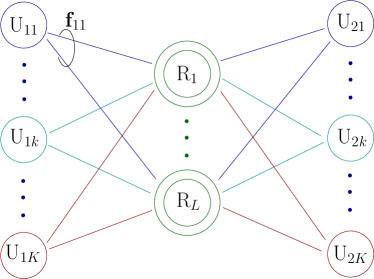
Fig. 1: A diagram of multiple user pair AF relay systems with $K$ pairs of users and $L$ relays.

II-A One-Way Relay System

In a one-way relay system, only one user in each pair transmits data to the other. Without loss of generality and for notational convenience, let us assume that $\mathrm{U}_{1k}$ is the transmitter and $\mathrm{U}_{2k}$ is the receiver, for all $k\in{\cal K}$.

II-A1 EH Phase (One-Way)

During EH phase, the relays harvest energy from the RF signal transmitted by the transmitters. Particularly, the RF power at the input of the EH circuit of $\mathrm{R}_{l}$ is [12]

$$P_{l}^{\text{RF,OW}}({\bf p})\triangleq\sum_{k\in{\cal K}}p_{1k}|f_{1kl}|^{2}$$ (1)

where $p_{ik}$, $(i=\{1,2\})$ is the transmit power at $\mathrm{U}_{ik}$ and ${\bf p}\triangleq[p_{11},...,p_{1K}]^{\mbox{\scriptsize T}}$. The EH power circuit converts $P_{l}^{\text{RF,OW}}({\bf p})$ to DC power used during the IT phase. Here, we consider a realistic RF-DC power converter, whose conversion efficiency is not a constant, introduced in [35]. Specifically, the harvested energy at $\mathrm{R}_{l}$ is

$$E_{l}^{\textrm{EH,OW}}(\tau,{\bf p})=\frac{\tau\bar{P}_{l}^{\text{DC}}}{1-\beta_{l}}\left(\frac{1}{1+\exp\bigl{(}-c_{l}(P_{l}^{\text{RF,OW}}({\bf p})-d_{l})\bigr{)}}-\beta_{l}\right)$$ (2)

where $\bar{P}_{l}^{\text{DC}}$ is the maximum power that can be harvested, $c_{l}$ and $d_{l}$ are parameters depending on the circuit specifications, and $\beta_{l}=(1+\exp(c_{l}d_{l}))^{-1}$.

II-A2 IT Phase (One-Way)

During IT phase, the remaining $(1-\tau)$ fraction of block time is divided into two equal-length time slots. In the first time slot, the transmitters send data to the relays. Let $x_{1k}$ denote the normalized complex symbol transmitted by $\mathrm{U}_{1k}$. The received signal at $\mathrm{R}_{l}$ is

$$\tilde{y}_{l}^{\textrm{OW}}=\sum_{k\in{\cal K}}\sqrt{p_{1k}}f_{1kl}x_{1k}+\tilde{n}_{l}$$ (3)

where $\tilde{n}_{l}$ is the additive white Gaussian noise (AWGN), i.e., $\tilde{{\bf n}}\sim\mathcal{CN}(0,\tilde{\sigma}^{2}\mathbf{I}_{L})$ with $\tilde{{\bf n}}\triangleq[\tilde{n}_{1},...,\tilde{n}_{L}]^{\mbox{\scriptsize T}}$. In the second time slot, the relays transmit the processed signal to the receivers. We denote by $w_{l}\in\mathbb{C}$ the complex weight coefficient used at $\mathrm{R}_{l}$, and let ${\bf w}\triangleq[w_{1},...,w_{L}]^{\mbox{\scriptsize T}}\in\mathbb{C}^{L\times 1}$. The received signal at $\mathrm{U}_{2k}$ is

$$y_{2k}^{\textrm{OW}} =\sum_{l\in{\cal L}}f_{2kl}w_{l}\tilde{y}_{l}^{\text{OW}}+n_{2k}=\underset{\textrm{desired\,signal}}{\underbrace{\sqrt{p_{1k}}{\bf f}_{2k}^{\mbox{\scriptsize T}}{\bf W}{\bf f}_{1k}x_{1k}}}+\underset{\textrm{interference}}{\underbrace{\sum_{j\in{\cal K}\backslash\{k\}}\sqrt{p_{1j}}{\bf f}_{2k}^{\mbox{\scriptsize T}}{\bf W}{\bf f}_{1j}x_{1j}}}+\underset{\textrm{noise}}{\underbrace{{\bf f}_{2k}^{\mbox{\scriptsize T}}{\bf W}\tilde{{\bf n}}+n_{2k}}}$$ (4)

where ${\bf W}\triangleq\text{diag}({\bf w})$, and $n_{2k}$ denotes the additive noise with $n_{2k}\sim\mathcal{CN}(0,\sigma^{2})$. The signal-to-interference-plus-noise ratio (SINR) at $\mathrm{U}_{2k}$ is

$$\gamma_{2k}^{\textrm{OW}}({\bf w},{\bf p}) =\frac{p_{1k}|{\bf f}_{2k}^{\mbox{\scriptsize T}}{\bf W}{\bf f}_{1k}|^{2}}{\sum_{j\in{\cal K}\backslash\{k\}}p_{1j}|{\bf f}_{2k}^{\mbox{\scriptsize T}}{\bf W}{\bf f}_{1j}|^{2}+\tilde{\sigma}^{2}||{\bf f}_{2k}^{\mbox{\scriptsize T}}{\bf W}||_{2}^{2}+\sigma^{2}}$$

$$=\frac{p_{1k}{\bf w}^{\mbox{\scriptsize H}}{\bf H}_{kk}{\bf w}}{\sum_{j\in{\cal K}\backslash\{k\}}p_{1j}{\bf w}^{\mbox{\scriptsize H}}{\bf H}_{kj}{\bf w}+{\bf w}^{\mbox{\scriptsize H}}{\bf G}_{2k}{\bf w}+\sigma^{2}}$$ (5)

where $\mathbf{h}_{kj}\triangleq({\bf f}_{2k}\odot{\bf f}_{1j})^{\mbox{\scriptsize T}}$, ${\bf H}_{kj}\triangleq\mathbf{h}_{kj}^{\mbox{\scriptsize H}}\mathbf{h}_{kj}$, and ${\bf G}_{ik}\triangleq\tilde{\sigma}^{2}\text{diag}\bigl{(}{\bf f}_{ik}^{\mbox{\scriptsize H}}\odot{\bf f}_{ik}^{\mbox{\scriptsize T}})$. Let $r_{ik}$ be the real transmit data rate at $\mathrm{U}_{ik}$, i.e., the effective information rate is $\frac{1-\tau}{2}r_{ik}$. For feasible transmission, the constraint

$$r_{1k}\leq\log(1+\gamma_{2k}^{\textrm{OW}}({\bf w},{\bf p})),\,\forall k\in{\cal K}$$ (6)

should hold. The purpose of introducing $\{r_{1k}\}_{k=1}^{K}$ is to determine the rate-dependent signal processing energy, which is discussed in detail next.

II-A3 Energy Consumption Model (One-Way)

We consider herein a relatively realistic energy consumption model which takes into account the dependence of PAs’ efficiency on the output power level [41, 20] as well as the dependence of signal processing operators on the transmit data rate [19]. In addition, for saving energy, a node can be idle (i.e., sleep mode) if it is neither receiving nor transmitting [16, 33]. In this spirit, let us first focus on the energy consumed by the users of pair $k$. Let $P_{ik}^{\textrm{idle}}$ denote the consumed power of $\mathrm{U}_{ik}$ in idle mode, which is assumed to be constant [16, 33]. Then, the energy consumed in this mode is

$$E_{k}^{\text{idle}}(\tau)=\frac{1-\tau}{2}P_{1k}^{\textrm{idle}}+\frac{1+\tau}{2}P_{2k}^{\textrm{idle}}.$$ (7)

On the other hand, for the clarity of description, we divide the power consumed in the active mode into three components: power consumed by the operating circuits, the amplifiers and signal processing. The first part includes the power consumed, e.g., by filters, mixers, etc, denoted by $P_{ik}^{\textrm{act,cir}}$ for $\mathrm{U}_{ik}$. It is modeled as a constant [42]. For the power consumed on the amplifiers, we consider a realistic model whose efficiency is given by [20, Eq. (2)]

$$\tilde{\epsilon}_{ik}=\epsilon_{ik}\sqrt{\frac{p_{ik}}{\bar{P}_{ik}}}$$ (8)

where $\epsilon_{ik}\in(0,1)$ is the maximum PA’s efficiency and $\bar{P}_{ik}$ is the maximum transmit power of $\mathrm{U}_{ik}$. From (8), the power consumed on the PA is

$$P_{ik}^{\textrm{amp}}=\frac{p_{ik}}{\tilde{\epsilon}_{ik}}=\varepsilon_{ik}\sqrt{p_{ik}}$$ (9)

where $\varepsilon_{ik}=\sqrt{\bar{P}_{ik}}/\epsilon_{ik}$. Finally, the power for signal processing is modeled as a linear function of data rate given by $P_{1k}^{\textrm{sp}}=(\rho_{1k}^{\textrm{en}}+\rho_{2k}^{\textrm{de}})r_{1k}$ where $\rho_{1k}^{\textrm{en}}$ and $\rho_{2k}^{\textrm{de}}$ represent power for encoder at $\mathrm{U}_{1k}$ and decoder at $\mathrm{U}_{2k}$, respectively. Their units are in W/(Gnats/s). In summary, the total energy consumed by pair $k$ during a block time is

$$E_{k}^{\textrm{OW}}(\tau,{\bf p},{\bf r}) =E_{k}^{\text{idle}}(\tau)+\frac{1+\tau}{2}(P_{1k}^{\textrm{amp}}+P_{1k}^{\textrm{act,cir}})+\frac{1-\tau}{2}(P_{1k}^{\textrm{sp}}+P_{2k}^{\textrm{act,cir}})$$

$$=\frac{1-\tau}{2}(\rho_{1k}^{\textrm{sp}}r_{1k}+P^{\prime}_{k})+\frac{1+\tau}{2}(\varepsilon_{1k}\sqrt{p_{1k}}+P^{\prime\prime}_{k})$$ (10)

where $\rho_{1k}^{\textrm{sp}}=\rho_{1k}^{\textrm{en}}+\rho_{2k}^{\textrm{de}}$, $P^{\prime}_{k}=P_{1k}^{\textrm{idle}}+P_{2k}^{\textrm{act,cir}}$, and $P^{\prime\prime}_{k}=P_{2k}^{\textrm{idle}}+P_{1k}^{\textrm{act,cir}}$, which are constant; ${\bf r}\triangleq[r_{11},...,r_{1K}]^{\mbox{\scriptsize T}}$.

We now describe the energy consumed by the relays. The radiated power at $\mathrm{R}_{l}$ is $P_{l}^{\text{rad}}({\bf p},{\bf w})\triangleq w_{l}^{\ast}\Bigl{(}{\textstyle\sum_{k\in{\cal K}}}p_{1k}|f_{1kl}|^{2}+\tilde{\sigma}^{2}\Bigr{)}w_{l}={\bf w}^{\mbox{\scriptsize H}}{\bf A}_{l}{\bf w}+\sum_{k\in{\cal K}}p_{1k}{\bf w}^{\mbox{\scriptsize H}}{\bf B}_{1kl}{\bf w}$ where ${\bf A}_{l}\triangleq\tilde{\sigma}^{2}\text{diag}(\mathbf{e}_{l})$ and ${\bf B}_{1kl}\triangleq|f_{1kl}|^{2}\text{diag}(\mathbf{e}_{l})$. Then, the total energy consumed at $\mathrm{R}_{l}$ is given by

$$E_{l}^{\textrm{R,OW}}(\tau,{\bf p},{\bf w})\triangleq\frac{1-\tau}{2}\frac{\sqrt{\bar{P}_{l}^{\text{R}}P_{l}^{\text{rad}}({\bf p},{\bf w})}}{\epsilon_{l}^{\text{R}}}+E_{l}^{\textrm{R,const}}$$ (11)

where $\epsilon_{l}^{\text{R}}\in(0,1)$ is the maximum PA’s efficiency and $\bar{P}_{l}^{\text{R}}$ is the maximum transmit power of $\mathrm{R}_{l}$. In (11), the first term is the energy consumed by the PA, and $E_{l}^{\textrm{R,const}}$ is the consumed energy for activating the basic functions which is constant [42]. Since the relays do not encode or decode data, the rate-dependent signal processing energy does not exist. Clearly, for successfully assisting the data transmission, the energy consumption cannot exceed harvesting or

$$E_{l}^{\text{R,OW}}(\tau,{\bf p},{\bf w})\leq E_{l}^{\textrm{EH,OW}}(\tau,{\bf p}),\,\forall l\in{\cal L}.$$ (12)

II-B Two-Way Relay System

In a two-way system, the relays assist the bi-directional communication of all pairs, i.e., both of the two users of each pair transmit and receive data.

II-B1 EH Phase (Two-Way)

The relays receive energy from the both two users of each pair. Hence, the RF power at the input of EH circuit of $\mathrm{R}_{l}$ is

$$P_{l}^{\text{RF,TW}}(\tilde{\mathbf{p}})\triangleq\sum_{k\in{\cal K}}\sum_{i=1}^{2}p_{ik}|f_{ikl}|^{2}$$ (13)

where $\tilde{\mathbf{p}}\triangleq[p_{11},p_{21},...,p_{1K},p_{2K}]^{\mbox{\scriptsize T}}$. Accordingly, the harvested energy at $\mathrm{R}_{l}$ is

$$E_{l}^{\textrm{EH,TW}}(\tau,\tilde{\mathbf{p}})=\frac{\tau\bar{P}_{l}^{\text{DC}}}{1-\beta_{l}}\left(\frac{1}{1+\exp\bigl{(}-c_{l}(P_{l}^{\text{RF,TW}}(\tilde{\mathbf{p}})-d_{l})\bigr{)}}-\beta_{l}\right).$$ (14)

II-B2 IT Phase (Two-Way)

In the first time slot of IT phase, all the users transmit their signals to the relays using the same frequency band. Particularly, the received signal at $\mathrm{R}_{l}$ is

$$\tilde{y}_{l}^{\textrm{TW}}=\sum_{k\in{\cal K}}\sum_{i=1}^{2}\sqrt{p_{ik}}f_{ikl}x_{ik}+\tilde{n}_{l}.$$ (15)

During the second time slot, the relays broadcast the processed signals to all the users. The received signal at $\mathrm{U}_{ik}$ is expressed as

$$y_{ik}^{\textrm{rec}} =\sum_{l\in{\cal L}}f_{ikl}w_{l}\tilde{y}_{l}^{\textrm{TW}}+n_{ik}=\sum_{j\in{\cal K}}\sum_{\hat{i}=1}^{2}\sqrt{p_{\hat{i}j}}{\bf f}_{ik}^{\mbox{\scriptsize T}}{\bf W}{\bf f}_{\hat{i}j}x_{\hat{i}j}+{\bf f}_{ik}^{\mbox{\scriptsize T}}{\bf W}\tilde{{\bf n}}+n_{ik}.$$ (16)

As with most of the related works (see [6, 8, 25, 18] and the references therein), we suppose that the self-interference can be completely canceled at the users (with the known CSI). Then the signal for decoding at $\mathrm{U}_{ik}$ reduces to

$$y_{ik}^{\textrm{TW}}=\underset{\textrm{desired\,signal}}{\underbrace{\sqrt{p_{\bar{i}k}}{\bf f}_{ik}^{\mbox{\scriptsize T}}{\bf W}{\bf f}_{\bar{i}k}x_{\bar{i}k}}}+\underset{\textrm{interference}}{\underbrace{\sum_{j\in{\cal K}\setminus\{k\}}\sum_{\hat{i}=1}^{2}\sqrt{p_{\hat{i}j}}{\bf f}_{ik}^{\mbox{\scriptsize T}}{\bf W}{\bf f}_{\hat{i}j}x_{\hat{i}j}}}+\underset{\textrm{noise}}{\underbrace{{\bf f}_{ik}^{\mbox{\scriptsize T}}{\bf W}\tilde{{\bf n}}+n_{ik}}}$$ (17)

where $\bar{i}=\{1,2\}\setminus\{i\}$. Thus the SINR at $\mathrm{U}_{ik}$ can be written as

$$\gamma_{ik}^{\textrm{TW}}({\bf w},\tilde{\mathbf{p}}) =\frac{p_{\bar{i}k}|{\bf f}_{ik}^{\mbox{\scriptsize T}}{\bf W}{\bf f}_{\bar{i}k}|^{2}}{\sum_{j\in{\cal K}\setminus\{k\}}\sum_{\hat{i}=1}^{2}p_{\hat{i}j}|{\bf f}_{ik}^{\mbox{\scriptsize T}}{\bf W}{\bf f}_{\hat{i}j}|^{2}+\tilde{\sigma}^{2}||{\bf f}_{ik}^{\mbox{\scriptsize T}}{\bf W}||_{2}^{2}+\sigma^{2}}$$

$$=\frac{p_{\bar{i}k}{\bf w}^{\mbox{\scriptsize H}}{\bf H}_{kk}{\bf w}}{\sum_{j\in{\cal K}\backslash\{k\}}\sum_{\hat{i}=1}^{2}p_{\hat{i}j}{\bf w}^{\mbox{\scriptsize H}}\tilde{{\bf H}}_{ik\hat{i}j}{\bf w}+{\bf w}^{\mbox{\scriptsize H}}{\bf G}_{ik}{\bf w}+\sigma^{2}}$$ (18)

where $\tilde{{\bf h}}_{ik\hat{i}j}\triangleq({\bf f}_{ik}\odot{\bf f}_{\hat{i}j})^{\mbox{\scriptsize T}}$ and $\tilde{{\bf H}}_{ik\hat{i}j}\triangleq\tilde{{\bf h}}_{ik\hat{i}j}^{\mbox{\scriptsize H}}\tilde{{\bf h}}_{ik\hat{i}j}$. We note that $\tilde{{\bf H}}_{ik\bar{i}k}=\tilde{{\bf H}}_{\bar{i}kik}={\bf H}_{kk}$. Similar to the one-way system, we need the following set of constraints for successful transmissions

$$r_{ik}\leq\log(1+\gamma_{\bar{i}k}^{\textrm{TW}}({\bf w},\tilde{\mathbf{p}})),\forall k\in{\cal K},i=\{1,2\}.$$ (19)

II-B3 Energy Consumption Model (Two-Way)

Different from the one-way relay system, the users in the two-way relay system are always active since each of them either transmits or receives during block time. In addition, the energy for the power amplifiers accounts on the both users of a pair, and the rate-dependent signal processing energy for pair $k$ is calculated based on the rate transmitted from $\mathrm{U}_{1k}$ and $\mathrm{U}_{2k}$. Thus the energy consumed by pair $k$ can be expressed as

$$E_{k}^{\textrm{TW}}(\tau,\tilde{\mathbf{p}},\tilde{\mathbf{r}}) \triangleq\underset{\textrm{energy\,for\,circuits}}{\underbrace{1\left(\sum_{i=1}^{2}P_{ik}^{\textrm{act,cir}}\right)}}+\underset{\textrm{energy\,for\,PAs}}{\underbrace{\frac{1+\tau}{2}\left(\sum_{i=1}^{2}P_{ik}^{\textrm{amp}}\right)}}+\underset{\textrm{energy\,for\,signal\,processing}}{\underbrace{\frac{1-\tau}{2}\left(\sum_{i=1}^{2}P_{ik}^{\text{sp}}\right)}}$$

$$=E_{k}^{\textrm{TW,cir}}+\frac{1+\tau}{2}\left(\sum_{i=1}^{2}\varepsilon_{ik}\sqrt{p_{ik}}\right)+\frac{1-\tau}{2}\left(\sum_{i=1}^{2}\rho_{ik}^{\textrm{sp}}r_{ik}\right)$$ (20)

where $E_{k}^{\textrm{TW,cir}}=1(\sum_{i=1}^{2}P_{ik}^{\textrm{act,cir}})$ is a constant, $\rho_{ik}^{\textrm{sp}}=\rho_{ik}^{\textrm{en}}+\rho_{\bar{i}k}^{\textrm{de}}$, and $\tilde{\mathbf{r}}\triangleq[r_{11},r_{21},...,r_{1K},r_{2K}]^{\mbox{\scriptsize T}}$.

For two-way relay $\mathrm{R}_{l}$, the radiated power is $P_{l}^{\text{rad,TW}}(\tilde{\mathbf{p}},{\bf w})\triangleq w_{l}^{\ast}\Bigl{(}{\textstyle\sum_{k\in{\cal K}}}\sum_{i=1}^{2}p_{ik}|f_{ikl}|^{2}+\tilde{\sigma}^{2}\Bigr{)}w_{l}={\bf w}^{\mbox{\scriptsize H}}{\bf A}_{l}{\bf w}+\sum_{k\in{\cal K}}\sum_{i=1}^{2}p_{ik}{\bf w}^{\mbox{\scriptsize H}}{\bf B}_{ikl}{\bf w}$. Then, the total consumed energy at $\mathrm{R}_{l}$ is

$$E_{l}^{\text{R,TW}}(\tau,\tilde{\mathbf{p}},{\bf w})\triangleq\frac{1-\tau}{2}\frac{\sqrt{\bar{P}_{l}^{\text{R}}P_{l}^{\text{rad,TW}}({\bf w},\tilde{\mathbf{p}})}}{\epsilon_{l}^{\text{R}}}+E_{l}^{\textrm{R,const}}.$$ (21)

Again, the following set of constraints on the harvested and consumed energy is required for successful relaying

$$E_{l}^{\text{R,TW}}(\tau,\tilde{\mathbf{p}},{\bf w})\leq E_{l}^{\textrm{EH,TW}}(\tau,\tilde{\mathbf{p}}),\,\forall l\in{\cal L}.$$ (22)

II-C Energy Efficiency Fairness Problems

We focus on the max-min EE. Here, the shared relays use energy contributed by the users for assisting data transmission, when each user exchanges information with the one in the same pair only. Hence, it is relevant to maintain the EE fairness (EEF) between the user pairs.

II-C1 EEF for One-Way Relay System

With the model specified in Section II-A and by definition, the individual EE of pair $k$ is given by

$$f_{k}^{\text{EE,OW}}(\tau,{\bf p},{\bf r})\triangleq\frac{\frac{1-\tau}{2}r_{1k}}{E_{k}^{\text{OW}}(\tau,{\bf p},{\bf r})},\ k\in{\cal K}$$ (23)

Thereby the problem of max-min EEF can be mathematically formulated as

$$\underset{{\bf p},{\bf w},{\bf r},\tau}{\text{maximize}}\ \min_{1\leq k\leq K}\ f_{k}^{\text{EE,OW}}(\tau,{\bf p},{\bf r})$$ (24a)

subject to $$\frac{1-\tau}{2}r_{1k}\geq Q_{1k},\,\forall k\in{\cal K}$$ (24b)

$$\textrm{EEF-OW}\triangleq\smash{\left\{\IEEEstrut[13]\right.}\hskip 51.21504pt 0<p_{1k}\leq\bar{P}_{1k},\,\forall k\in{\cal K}$$ (24c)

$$P_{l}^{\text{rad}}({\bf p},{\bf w})\leq\bar{P}_{l}^{\text{R}},\,\forall l\in{\cal L}$$ (24d)

$$\eqref{eq:rate},\eqref{eq:EnergyCons}.$$ (24e)

Constraint (24b) guarantees the quality of service (QoS) for each user pair, where $Q_{1k}>0$ is a predefined threshold. (24c) and (24d) represent the transmit power constraints at the transmitters and the relays, respectively.

II-C2 EEF for Two-Way Relay System

Similarly, we obtain the problem of max-min EEF for the two-way system as

$$\underset{\tilde{\mathbf{p}},{\bf w},\tilde{\mathbf{r}},\tau}{\text{maximize}}\ \min_{1\leq k\leq K}\ f_{k}^{\text{EE,TW}}(\tau,\tilde{\mathbf{p}},\tilde{\mathbf{r}})\triangleq\frac{\frac{1-\tau}{2}\sum_{i=1}^{2}r_{ik}}{E_{k}^{\textrm{TW}}(\tau,\tilde{\mathbf{p}},\tilde{\mathbf{r}})}$$ (25a)

subject to $$\frac{1-\tau}{2}r_{ik}\geq Q_{ik},\,\forall k\in{\cal K},i=1,2$$ (25b)

$$\textrm{EEF-TW}\triangleq\smash{\left\{\IEEEstrut[13]\right.}\hskip 51.21504pt 0<p_{ik}\leq\bar{P}_{ik},\,\forall k\in{\cal K},i=1,2$$ (25c)

$$P_{l}^{\text{rad,TW}}(\tilde{\mathbf{p}},{\bf w})\leq\bar{P}_{l}^{\text{R}},\,\forall l\in{\cal L}$$ (25d)

$$\eqref{eq:rate-tw},\eqref{eq:EnergyCons-tw}.$$ (25e)

In this work, we assume that the feasible sets of EEF-OW and EEF-TW are nonempty. The objectives in EEF-OW and EEF-TW are nonsmooth nonconvex—the numerators of the fractions are linear, but the denominators are nonconvex. Also, the feasible sets are nonconvex. Hence the problems are intractable and it is impossible to transform the problems into the equivalent convex ones. Like many studies on wireless communication designs [30, 18, 24, 27], we aim at finding approximate, but efficient, solutions to these problems.

III The Proposed Algorithms for Solving EEF-OW and EEF-TW

In this section, we propose algorithms for solving EEF-OW and EEF-TW based on the inner approximation (IA) framework [37, 38], which is an efficient approach widely used for dealing with nonconvex programs. First, the general principles of the IA and the useful approximation functions are provided. Then, the IA-based algorithms solving EEF-OW and EEF-TW are presented, followed by the convergence discussion. Finally, the approach arriving at the SOCP approximations is provided.

III-A Useful Approximate Formulations

For exposition purpose, we first provide some approximate formulations which are used to devise proposed solutions. Generally the basic idea of IA is to successively approximate a nonconvex set to inner convex ones. Specifically, let $h(\mathbf{x})\leq 0$ be a nonconvex constraint where $h(\mathbf{x}):\mathbb{C}^{n}\rightarrow\mathbb{R}$ and $h(\mathbf{x})$ is continuously differentiable. An inner approximation is obtained by replacing $h(\mathbf{x})$ by a convex upper bound $\tilde{h}(\mathbf{x};g(\mathbf{x}^{\prime}))$, i.e., $h(\mathbf{x})\leq\tilde{h}(\mathbf{x};g(\mathbf{x}^{\prime}))$, where $g(\mathbf{x}):\mathbb{C}^{n}\rightarrow\mathbb{C}^{m}$ is a parameter vector and $\mathbf{x}^{\prime}$ is some feasible point. Function $\tilde{h}(\mathbf{x};g(\mathbf{x}^{\prime}))$ must satisfy the following conditions

$$h(\mathbf{x})=\tilde{h}(\mathbf{x};g(\mathbf{x})),\,\nabla_{\mathbf{x}^{\ast}}h(\mathbf{x})=\nabla_{\mathbf{x}^{\ast}}\tilde{h}(\mathbf{x};g(\mathbf{x}))$$ (26)

where $\nabla_{\mathbf{x}^{\ast}}h()$ denotes the gradient of $h()$ with respect to the complex conjugate of $\mathbf{x}$. If $\mathbf{x}$ is a real vector, then $\nabla_{\mathbf{x}^{\ast}}h()$ is simply replaced by $\nabla_{\mathbf{x}}h()$. The approximations presented next follow these principles.

III-A1 Approximation for Bilinear Function

Consider nonconvex constraint $x_{1}x_{2}\leq y$ where $(x_{1},x_{2},y)\in\mathbb{R}_{++}^{3}$. An approximation of bilinear function $x_{1}x_{2}$ is given by [37, Lem. 3.5]

$$x_{1}x_{2}\leq h^{\textrm{bi}}(x_{1},x_{2};\lambda)\triangleq 0.5\left(\lambda x_{1}^{2}+\frac{x_{2}^{2}}{\lambda}\right)$$ (27)

where $\lambda=\frac{x^{\prime}_{2}}{x^{\prime}_{1}}$. We remark that the bilinear function can be rewritten as difference-of-convex ones, e.g., $x_{1}x_{2}=0.25(x_{1}+x_{2})^{2}-0.25(x_{1}-x_{2})^{2}=0.5(x_{1}+x_{2})^{2}-0.5(x_{1}^{2}+x_{2}^{2})=0.5(x_{1}^{2}+x_{2}^{2})-0.5(x_{1}-x_{2})^{2}$. Then the approximates can be obtained by using the first order Taylor series approximation of the nonconvex parts. Herein, we use (27) for problems EEF-OW and EEF-TW, since we numerically observe that with (27), the iterative procedures require fewer number of iterations for convergence (see Fig. 3(a) for the numerical example).

III-A2 Approximation for Fractional-Linear Function

Consider nonconvex constraint $\frac{x_{1}}{x_{2}}\leq y$ where $(x_{1},x_{2},y)\in\mathbb{R}_{++}^{3}$. In light of (27), an approximation of fractional-linear function $\frac{x_{1}}{x_{2}}$ can be obtained as

$$\frac{x_{1}}{x_{2}}\leq h^{\textrm{frac}}(x_{1},x_{2};\lambda)\triangleq 0.5\left(\lambda x_{1}^{2}+\frac{1}{\lambda x_{2}^{2}}\right)$$ (28)

where $\lambda=\frac{1}{x^{\prime}_{1}x^{\prime}_{2}}$. We note that constraint $h^{\textrm{frac}}(x_{1},x_{2};\lambda)\leq y$ can be expressed by the following two second-order cone (SOC) ones

$$0.5\left(\lambda x_{1}^{2}+\frac{z^{2}}{\lambda}\right)\leq y,\,1\leq x_{2}z.$$ (29)

III-A3 Approximation for Quadratic-over-Linear Function

Consider concave function $h(\mathbf{x},z;\mathbf{A})\triangleq-\frac{\mathbf{x}^{\mbox{\scriptsize H}}\mathbf{A}\mathbf{x}}{z}$ where $\mathbf{x}\in\mathbb{C}^{n}$, $z\in\mathbb{R}_{++}$, and $\mathbf{A}\succeq 0$. We can use the first order Taylor series to obtain a convex upper bound of $h(\mathbf{x},z;\mathbf{A})$ given as

$$h^{\textrm{qol}}(\mathbf{x},z;\mathbf{x}^{\prime},z^{\prime};\mathbf{A}) \triangleq h(\mathbf{x}^{\prime},z^{\prime};\mathbf{A})+\left\langle[\nabla_{\mathbf{x}^{\ast}}h(\mathbf{x}^{\prime},z^{\prime};\mathbf{A}),\nabla_{z}h(\mathbf{x}^{\prime},z^{\prime};\mathbf{A})]^{\mbox{\scriptsize T}},[\mathbf{x}-\mathbf{x}^{\prime},z-z^{\prime}]^{\mbox{\scriptsize T}}\right\rangle$$

$$=\frac{(\mathbf{x}^{\prime})^{\mbox{\scriptsize H}}\mathbf{A}\mathbf{x}^{\prime}}{(z^{\prime})^{2}}z-\frac{2\Re(({\bf x}^{\prime})^{\mbox{\scriptsize H}}\mathbf{A}{\bf x})}{z^{\prime}}.$$ (30)

III-A4 Approximation for Logarithmic Function

Consider logarithmic function $h(x)\triangleq\log(x)$ where $x\in\mathbb{R}_{++}$. An approximated function of $h(x)$ is given by

$$h(x)\leq h^{\textrm{log}}(x;x^{\prime})\triangleq\log(x^{\prime})-1+\frac{x}{x^{\prime}}.$$ (31)

III-A5 Approximation for Power Function

Consider power function $h(x;m)\triangleq-x^{m}$ where $x\in\mathbb{R}_{++}$. Here, we only focus on the cases $m<0$ or $m>1$ where $h(x;m)$ is concave. Its convex approximation is given by

$$h(x;m)\leq h^{\textrm{po}}(x;x^{\prime};m)\triangleq(m-1)(x^{\prime})^{m}-m(x^{\prime})^{m-1}x.$$ (32)

III-B Solution for EEF-OW

Directly applying IA to (24) is difficult, since the nonconvex parts here are not explicitly exposed. As a necessary step, we translate (24) into an equivalent, but more tractable, formulation. We first introduce variable $\eta>0$ and arrive at the epigraph form of (24) given as

$$\underset{{\bf p},{\bf w},{\bf r},\tau,\eta}{\text{minimize}}\ \eta$$ (33a)

subject to $$f_{k}^{\text{EE,OW}}(\tau,{\bf p},{\bf r})\geq\eta^{-1},\,\forall k\in{\cal K}$$ (33b)

$$\eqref{eq:rate},\eqref{eq:EnergyCons},\eqref{eq:QoS},\eqref{eq:source:txpower},\eqref{eq:relaypow}.$$ (33c)

Here the nonconvex parts include (6), (12), (24d), and (33b).

III-B1 Changes of Variables

We now make some changes of variables. Specifically, we will denote $q_{ik}=\frac{1}{p_{ik}}$, $\forall k\in{\cal K},i=1,2$, and turn the nonconvex products of linear and quadratic functions, e.g., $p_{1k}{\bf w}^{\mbox{\scriptsize H}}{\bf H}_{kk}{\bf w}$, into the quadratic-over-linear functions. We also define $\tilde{\tau}=\frac{1+\tau}{1-\tau}$, i.e., $\tau=\frac{\tilde{\tau}-1}{\tilde{\tau}+1}$. It is important to note that these changes of variables still preserve the convexity in (24b) and (24c) as well as turn nonconvex constraint (24d) into a convex one. In addition, they make (6), (12), and (33b) become more convenient to handle, as shown next.

III-B2 Transformation of (6)

By introducing new variables $\{v_{k}\}_{k=1}^{K}$ and $\{s_{k}\}_{k=1}^{K}$, we can equivalently represent (6) by the following set of constraints

$$r_{1k}\leq\log(1+v_{k}),\,\forall k\in{\cal K}$$ (34)

$$\sum_{j\in{\cal K}\backslash\{k\}}\frac{{\bf w}^{\mbox{\scriptsize H}}{\bf H}_{kj}{\bf w}}{q_{1j}}+{\bf w}^{\mbox{\scriptsize H}}{\bf G}_{2k}{\bf w}+\sigma^{2}\leq s_{k},\,\forall k\in{\cal K}$$ (35)

$$s_{k}v_{k}\leq\frac{{\bf w}^{\mbox{\scriptsize H}}{\bf H}_{kk}{\bf w}}{q_{1k}},\,\forall k\in{\cal K}.$$ (36)

Here, only (36) is nonconvex which contains bilinear and quadratic-over-linear functions.

III-B3 Transformation of (12)

We first rewrite (12) with the change variables as

$$\tilde{\varepsilon}_{l}\sqrt{{\bf w}^{\mbox{\scriptsize H}}{\bf A}_{l}{\bf w}+\sum_{k\in{\cal K}}\frac{{\bf w}^{\mbox{\scriptsize H}}{\bf B}_{1kl}{\bf w}}{q_{1k}}} \leq\frac{\hat{\beta}_{l}(\tilde{\tau}-1)}{1+\alpha_{l}\exp\bigl{(}-c_{l}\sum_{k\in{\cal K}}\frac{|f_{1kl}|^{2}}{q_{1k}}\bigr{)}}-\bar{\beta}_{l}\tilde{\tau}+\check{\beta}_{l},\!\forall l\in\mathcal{L}$$

where $\tilde{\varepsilon}_{l}=\sqrt{\bar{P}_{l}^{\text{R}}}/\epsilon_{l}^{\text{R}}$, $\hat{\beta}_{l}=\frac{\bar{P}_{l}^{\text{DC}}}{1-\beta_{l}}$, $\bar{\beta}_{l}=\beta_{l}\hat{\beta}_{l}+E_{l}^{\textrm{R,const}}$, $\check{\beta}_{l}=\bar{\beta}_{l}-2E_{l}^{\textrm{R,const}}$ and $\alpha_{l}=\exp(c_{l}d_{l})$. Also, to reveal the hidden convexity in the constraint, we introduce new variables $\{u_{l}\}_{l=1}^{L}$ and $\{t_{l}\}_{l=1}^{L}$, and equivalently rewrite (12) as

$$\sum_{k\in{\cal K}}\frac{{\bf w}^{\mbox{\scriptsize H}}{\bf B}_{1kl}{\bf w}}{q_{1k}}\leq u_{l}^{2},\!\forall l\in\mathcal{L}$$ (37)

$$\log(\tilde{\tau}-t_{l}-1)-\log(\alpha_{l}t_{l})+\sum_{k\in{\cal K}}\frac{c_{l}|f_{1kl}|^{2}}{q_{1k}}\geq 0,\!\forall l\in\mathcal{L}$$ (38)

$$\tilde{\varepsilon}_{l}\sqrt{{\bf w}^{\mbox{\scriptsize H}}{\bf A}_{l}{\bf w}+u_{l}^{2}}\leq\hat{\beta}_{l}t_{l}-\bar{\beta}_{l}\tilde{\tau}+\check{\beta}_{l},\!\forall l\in\mathcal{L}.$$ (39)

The nonconvex parts are in (37) and (38) including the power and the logarithmic functions.

III-B4 Transformation of (33b)

Constraint (33b) is rewritten as

$$\rho_{1k}^{\text{sp}}+\frac{P^{\prime}_{k}}{r_{1k}}+\frac{\tilde{\tau}}{r_{1k}}\Bigl{(}\frac{\varepsilon_{1k}}{\sqrt{q_{1k}}}+P^{\prime\prime}_{k}\Bigr{)}\leq\eta,\!\forall k\in\mathcal{K},$$ (40)

which is equivalently represented as

$$\frac{\tilde{\tau}}{r_{1k}}\leq z_{k}^{2},\!\forall k\in\mathcal{K}$$ (41)

$$\rho_{1k}^{\text{sp}}+\frac{P^{\prime}_{k}}{r_{1k}}+\varepsilon_{1k}\frac{z_{k}^{2}}{\sqrt{q_{1k}}}+P^{\prime\prime}_{k}z_{k}^{2}\leq\eta,\!\forall k\in\mathcal{K}$$ (42)

where $\{z_{k}\}_{k=1}^{K}$ are newly introduced variables. We remark that function $z_{k}^{2}/\sqrt{q_{1k}}$ is convex (see Appendix -B for the proof), and so is (42). Also, (41) can be rewritten as $\frac{1}{r_{1k}}\leq\frac{z_{k}^{2}}{\tilde{\tau}}$ where the nonconvex part is quadratic-over-linear.

With the above transformations, (33) can be reformulated as

$$\underset{\begin{subarray}{c}\mathbf{q},{\bf w},{\bf r},\tilde{\tau},\eta\\ \mathbf{v},\mathbf{s},\mathbf{u},\mathbf{t},\mathbf{z}\end{subarray}}{\text{minimize}}\ \eta$$ (43a)

subject to $$r_{1k}\geq(1+\tilde{\tau})Q_{1k},\,\forall k\in{\cal K}$$ (43b)

$$q_{1k}\geq 1/\bar{P}_{1k},\,\forall k\in{\cal K}$$ (43c)

$${\bf w}^{\mbox{\scriptsize H}}{\bf A}_{l}{\bf w}+\sum_{k\in{\cal K}}\frac{{\bf w}^{\mbox{\scriptsize H}}{\bf B}_{1kl}{\bf w}}{q_{1k}}\leq\bar{P}_{l}^{\text{R}},\,\forall l\in{\cal L}$$ (43d)

$$\eqref{eq:rate-1},\eqref{eq:rate-2},\eqref{eq:rate-3},\eqref{eq:Econst-1},\eqref{eq:Econst-2},\eqref{eq:Econst-3},\eqref{eq:eesource-1},\eqref{eq:eesource-2}$$ (43e)

where $\mathbf{q}\triangleq[q_{1k},...,q_{1K}]^{\mbox{\scriptsize T}}$, $\mathbf{v}\triangleq[v_{1},...,v_{K}]^{\mbox{\scriptsize T}}$, $\mathbf{s}\triangleq[s_{1},...,s_{K}]^{\mbox{\scriptsize T}}$, $\mathbf{u}\triangleq[u_{1},...,u_{L}]^{\mbox{\scriptsize T}}$, $\mathbf{t}\triangleq[t_{1},...,t_{L}]^{\mbox{\scriptsize T}}$, and $\mathbf{z}\triangleq[z_{1},...,z_{K}]^{\mbox{\scriptsize T}}$; (43b), (43c), and (43d) are respectively the versions of (24b), (24c), and (24d) after change of variables. The equivalence here is in the sense of optimality (see the proof in Appendix -A).

We are now ready to use IA for solving (43). Specifically, by applying the approximate formulations provided in Section III-A to the nonconvex parts in (43), we obtain the following convex approximation of (43) solved at iteration $n+1$

$$\underset{\bm{\psi}}{\text{minimize}}\ \eta$$ (44a)

subject to $$h^{\textrm{bi}}(s_{k},v_{k};\frac{v_{k}^{(n)}}{s_{k}^{(n)}})+h^{\textrm{qol}}({\bf w},q_{1k};{\bf w}^{(n)},q_{1k}^{(n)};{\bf H}_{kk})\leq 0,\,\forall k\in{\cal K}$$ (44b)

$$\sum_{k\in{\cal K}}\frac{{\bf w}^{\mbox{\scriptsize H}}{\bf B}_{1kl}{\bf w}}{q_{1k}}+h^{\textrm{po}}(u_{l};u_{l}^{(n)};2)\leq 0,\,\forall l\in{\cal L}$$ (44c)

$$\log(\tilde{\tau}-t_{l}-1)\geq h^{\textrm{log}}(\alpha_{l}t_{l};\alpha_{l}t_{l}^{(n)})+\sum_{k\in{\cal K}}c_{l}|f_{1kl}|^{2}h^{\textrm{po}}(q_{1k};q_{1k}^{(n)};-1),\!\forall l\in\mathcal{L}$$ (44d)

$$\frac{1}{r_{1k}}+h^{\textrm{qol}}(z_{k},\tilde{\tau};z_{k}^{(n)},\tilde{\tau}^{(n)};1)\leq 0,\!\forall k\in\mathcal{K}$$ (44e)

$$\eqref{eq:rate-1},\eqref{eq:rate-2},\eqref{eq:Econst-3},\eqref{eq:eesource-2},\eqref{eq:QoS-1},\eqref{eq:source:txpower-1},\eqref{eq:relaypow-1}$$ (44f)

where $\bm{\psi}\triangleq[\mathbf{q}^{\mbox{\scriptsize T}},{\bf w}^{\mbox{\scriptsize T}},{\bf r}^{\mbox{\scriptsize T}},\tilde{\tau},\eta,\mathbf{v}^{\mbox{\scriptsize T}},\mathbf{s}^{\mbox{\scriptsize T}},\mathbf{u}^{\mbox{\scriptsize T}},\mathbf{t}^{\mbox{\scriptsize T}},\mathbf{z}^{\mbox{\scriptsize T}}]^{\mbox{\scriptsize T}}$ and $\bm{\psi}^{(n)}$ is some feasible point of (43).

Algorithm 1 The Proposed Method Solving EEF-OW

1:  Initialization: Set $n\coloneqq 0$, $n^{\prime}\coloneqq 0$, and randomly generate a feasible point $\bm{\psi}^{(0)}$ of (45).

2:  repeat {Finding a feasible point of (43)}

3:     Solve $\underset{\bm{\psi}\in\mathcal{S}(\bm{\psi}^{(n^{\prime})})}{\text{minimize}}\ \eta+b\sum_{k\in{\cal K}}[(1+\tilde{\tau})Q_{1k}-r_{1k}]^{+}$, denote the optimal by $\bm{\psi}_{\text{fe}}^{\ast}$.

4:     Update $n^{\prime}:=n^{\prime}+1$, $\bm{\psi}^{(n^{\prime})}:=\bm{\psi}_{\text{fe}}^{\ast}$.

5:  until $\sum_{k\in{\cal K}}[(1+\tilde{\tau}^{\ast})Q_{1k}-r_{1k}^{\ast}]^{+}=0$.

6:  Set $\bm{\psi}^{(0)}\coloneqq\bm{\psi}^{(n^{\prime})}$.

7:  repeat {Solving (43)}

8:     Obtain the optimal point of (44), denoted by $\bm{\psi}^{\ast}$.

9:     Update $n:=n+1$, $\bm{\psi}^{(n)}:=\bm{\psi}^{\ast}$.

10:  until convergence or predefined number of iterations.

11:  Output (solution for EEF-OW): $\tau\coloneqq\frac{\tilde{\tau}^{(n)}-1}{\tilde{\tau}^{(n)}+1}$, $\mathbf{w}\coloneqq\mathbf{w}^{(n)}$, $p_{1k}\coloneqq 1/q_{1k}^{(n)}$ for all $k\in\mathcal{K}$.

III-B5 Finding Initial Feasible Points

A feasible point of (43) is required for starting the IA procedure, which is difficult to find due to the QoS constraints. Here we provide an efficient heuristic method inspired by [43],[44, Section 3.2] to overcome this issue. The idea is to allow the QoS constraints to be violated, and the violation is penalized. Particularly, let us consider the following modification of (43)

$$\underset{\bm{\psi}\in\mathcal{S}}{\text{minimize}}\ \eta+b\sum_{k\in{\cal K}}[(1+\tilde{\tau})Q_{1k}-r_{1k}]^{+}$$ (45)

where $b>0$ is a penalty parameter; $\mathcal{S}\triangleq\{\bm{\psi}|\eqref{eq:rate-1}\textrm{--}\eqref{eq:eesource-2},\eqref{eq:source:txpower-1},\eqref{eq:relaypow-1}\}$. Finding feasible points of (45) is easy as follows. We first randomly generate $\tau^{(0)}\in(0,1)$, $0<p_{1k}^{(0)}\leq\bar{P}_{1k}$, and ${\bf w}^{(0)}\in\mathbb{C}^{L\times 1}$, then (if necessary) scale ${\bf w}^{(0)}$ so that (12) and (24d) are satisfied. Based on $(\tau^{(0)},p_{1k}^{(0)},{\bf w}^{(0)})$, ${\bf r}^{(0)},\mathbf{v}^{(0)},\mathbf{s}^{(0)},\mathbf{u}^{(0)},\mathbf{t}^{(0)}$, and $\mathbf{z}^{(0)}$ are determined by setting (34), (35), (36), (37), (39), and (41) to be equality. With $\bm{\psi}^{(0)}$, we can start an iterative IA procedure for solving (45). Intuitively, the penalty term in (45) would force $\{(1+\tilde{\tau})Q_{k}-r_{1k}\}$ to decrease. Once $(1+\tilde{\tau})Q_{k}-r_{1k}\leq 0$ for all $k$, i.e., the penalty term is zero, producing a feasible point of (43).

In summary, we outline the proposed method for solving EEF-OW in Algorithm 1. In line 3, $\mathcal{S}(\bm{\psi}^{(n)})\triangleq\{\bm{\psi}|\eqref{eq:rate-1},\eqref{eq:rate-2},\eqref{eq:Econst-3},\eqref{eq:eesource-2},\eqref{eq:source:txpower-1},\eqref{eq:relaypow-1},\eqref{eq:appr-ow-1}\textrm{--}\eqref{eq:appr-ow-4}\}$ is an approximate convex set of $\mathcal{S}$ corresponding to $\bm{\psi}^{(n)}$.

III-C Solution for EEF-TW

The procedure for finding a solution of EEF-TW is similar to the one presented in the previous subsection. So, for the sake of brevity, only the main steps are presented. We first arrive at the epigraph form of EEF-TW given by

$$\underset{\tilde{\mathbf{p}},{\bf w},\tilde{\mathbf{r}},\tau,\tilde{\eta}}{\text{minimize}}\ \tilde{\eta}$$ (46a)

subject to $$f_{k}^{\text{EE,TW}}(\tau,\tilde{\mathbf{p}},\tilde{\mathbf{r}})\geq\tilde{\eta}^{-1},\,\forall k\in{\cal K}$$ (46b)

$$\eqref{eq:rate-tw},\eqref{eq:EnergyCons-tw},\eqref{eq:QoS-tw},\eqref{eq:source:txpower-tw},\eqref{eq:relaypow-tw}.$$ (46c)

We focus on the nonconvex convexity induced by (19), (22), (25d), and (46b). Again, by using the change of variables in Section III-B1 and introducing additional variables, we transform (46) into the following equivalent problem

$$\underset{\begin{subarray}{c}\tilde{\mathbf{q}},{\bf w},\tilde{\mathbf{r}},\tilde{\tau},\tilde{\eta}\\ \tilde{\mathbf{v}},\tilde{\mathbf{s}},\mathbf{u},\mathbf{t},\mathbf{z}\end{subarray}}{\text{minimize}}\ \tilde{\eta}$$ (47a)

subject to $$r_{ik}\geq(1+\tilde{\tau})Q_{ik},\,\forall k\in{\cal K},i=\{1,2\}$$ (47b)

$$q_{ik}\geq 1/\bar{P}_{ik},\,\forall k\in{\cal K},i=\{1,2\}$$ (47c)

$${\bf w}^{\mbox{\scriptsize H}}{\bf A}_{l}{\bf w}+\sum_{k\in{\cal K}}\sum_{i=1}^{2}\frac{{\bf w}^{\mbox{\scriptsize H}}{\bf B}_{ikl}{\bf w}}{q_{ik}}\leq\bar{P}_{l}^{\text{R}},\,\forall l\in{\cal L}$$ (47d)

$$r_{ik}\leq\log(1+v_{\bar{i}k}),\!\forall k\in{\cal K},i=\{1,2\},\bar{i}=\{1,2\}\setminus\{i\}$$ (47e)

$$\sum_{j\in{\cal K}\backslash\{k\}}\sum_{\hat{i}=1}^{2}\frac{{\bf w}^{\mbox{\scriptsize H}}\tilde{{\bf H}}_{ik\hat{i}j}{\bf w}}{q_{\hat{i}j}}+{\bf w}^{\mbox{\scriptsize H}}{\bf G}_{ik}{\bf w}+\sigma^{2}\leq s_{ik},\!\forall k\in{\cal K},i=1,2$$ (47f)

$$s_{ik}v_{ik}\leq\frac{{\bf w}^{\mbox{\scriptsize H}}{\bf H}_{kk}{\bf w}}{q_{\bar{i}k}},\!\forall k\in{\cal K},i=\{1,2\},\bar{i}=\{1,2\}\setminus\{i\}$$ (47g)

$$\sum_{k\in{\cal K}}\sum_{i=1}^{2}\frac{{\bf w}^{\mbox{\scriptsize H}}{\bf B}_{ikl}{\bf w}}{q_{ik}}\leq u_{l}^{2},\!\forall l\in\mathcal{L}$$ (47h)

$$\log(\tilde{\tau}-t_{l}-1)-\log(\alpha_{l}t_{l})+c_{l}\sum_{k\in{\cal K}}\sum_{i=1}^{2}\frac{|f_{ikl}|^{2}}{q_{ik}}\geq 0,\!\forall l\in\mathcal{L}$$ (47i)

$$\tilde{\varepsilon}_{l}\sqrt{{\bf w}^{\mbox{\scriptsize H}}{\bf A}_{l}{\bf w}+u_{l}^{2}}\leq\hat{\beta}_{l}t_{l}-\bar{\beta}_{l}\tilde{\tau}+\check{\beta}_{l},\!\forall l\in\mathcal{L}$$ (47j)

$$\frac{\tilde{\tau}}{\sum_{i=1}^{2}r_{ik}}\leq z_{k}^{2},\!\forall k\in{\cal K}$$ (47k)

$$\left(\frac{1}{\sum_{i=1}^{2}r_{ik}}+z_{k}^{2}\right)E_{k}^{\textrm{TW,cir}}+\left(\sum_{i=1}^{2}\varepsilon_{ik}\frac{z_{k}^{2}}{\sqrt{q_{ik}}}\right)+\frac{\sum_{i=1}^{2}\rho_{ik}^{\textrm{sp}}r_{ik}}{\sum_{i=1}^{2}r_{ik}}\leq\tilde{\eta},\!\forall k\in{\cal K}$$ (47l)

where $\tilde{\mathbf{v}}\triangleq[v_{11},v_{21},...,v_{1K},v_{2K}]^{\mbox{\scriptsize T}}$, $\tilde{\mathbf{s}}\triangleq[s_{11},s_{21},...,s_{1K},s_{2K}]^{\mbox{\scriptsize T}}$. Similar to EEF-OW, the equivalence here is in the sense of optimality. In (47), the nonconvex parts include (47g), (47h), (47i), (47k), (47l), which can also be approximated using the approximate functions provided in Section III-A. By doing so, we arrive at the convex approximation problem given as

$$\underset{\tilde{\bm{\psi}}}{\text{minimize}}\quad\tilde{\eta}$$ (48a)

subject to

$$h^{\textrm{bi}}\left(s_{ik},v_{ik};v_{ik}^{(n)}/s_{ik}^{(n)}\right)+h^{\textrm{qol}}({\bf w},q_{\bar{i}k};{\bf w}^{(n)},q_{\bar{i}k}^{(n)};{\bf H}_{kk})\leq 0,\forall k\in{\cal K},i=\{1,2\},\bar{i}=\{1,2\}\setminus\{i\}$$ (48b)

$$\sum_{k\in{\cal K}}\sum_{i=1}^{2}\frac{{\bf w}^{\mbox{\scriptsize H}}{\bf B}_{ikl}{\bf w}}{q_{ik}}+h^{\textrm{po}}(u_{l};u_{l}^{(n)};2)\leq 0,\forall l\in\mathcal{L}$$ (48c)

$$\log(\tilde{\tau}-t_{l}-1)\geq h^{\textrm{log}}(\alpha_{l}t_{l};\alpha_{l}t_{l}^{(n)})+\sum_{k\in{\cal K}}\sum_{i=1}^{2}c_{l}|f_{ikl}|^{2}h^{\textrm{po}}(q_{ik};q_{ik}^{(n)};-1),\forall l\in\mathcal{L}$$ (48d)

$$\frac{1}{\sum_{i=1}^{2}r_{ik}}+h^{\textrm{qol}}(z_{k},\tilde{\tau};z_{k}^{(n)},\tilde{\tau}^{(n)};1)\leq 0,\forall k\in{\cal K}$$ (48e)

$$\left(\frac{1}{\sum_{i=1}^{2}r_{ik}}+z_{k}^{2}\right)E_{k}^{\textrm{TW,cir}}+\left(\sum_{i=1}^{2}\varepsilon_{ik}\frac{z_{k}^{2}}{\sqrt{q_{ik}}}\right)$$

$$\hskip 28.45274pt+h^{\textrm{frac}}\left(\sum_{i=1}^{2}\rho_{ik}^{\textrm{sp}}r_{ik},\sum_{i=1}^{2}r_{ik};\frac{1}{(\sum_{i=1}^{2}\rho_{ik}^{\textrm{sp}}r_{ik}^{(n)})(\sum_{i=1}^{2}r_{ik}^{(n)})}\right)\leq\tilde{\eta},\forall k\in{\cal K}$$ (48f)

$$\eqref{eq:qos-2-tw},\eqref{eq:sourcepow-2-tw},\eqref{eq:relaypow-2-tw},\eqref{eq:rate-2-1-tw},\eqref{eq:rate-2-2-tw},\eqref{eq:eh-2-3-tw}$$ (48g)

where $\tilde{\bm{\psi}}\triangleq[\tilde{\mathbf{q}}^{\mbox{\scriptsize T}},{\bf w}^{\mbox{\scriptsize T}},\tilde{\mathbf{r}}^{\mbox{\scriptsize T}},\tilde{\tau},\tilde{\eta},\tilde{\mathbf{v}}^{\mbox{\scriptsize T}},\tilde{\mathbf{s}}^{\mbox{\scriptsize T}},\mathbf{u}^{\mbox{\scriptsize T}},\mathbf{t}^{\mbox{\scriptsize T}},\mathbf{z}]^{\mbox{\scriptsize T}}$ and $\tilde{\bm{\psi}}^{(n)}$ is a feasible point of (47). Finally, for finding initial feasible points of (47), we use a similar technique as that in Section III-B5.

The proposed procedure for solving EEF-TW is outlined in Algorithm 2. In line 3, $\tilde{\mathcal{S}}(\tilde{\bm{\psi}}^{(n)})\triangleq\{\tilde{\bm{\psi}}|\eqref{eq:qos-2-tw},\eqref{eq:sourcepow-2-tw},\eqref{eq:relaypow-2-tw},\eqref{eq:rate-2-1-tw},\eqref{eq:rate-2-2-tw},\eqref{eq:eh-2-3-tw},\eqref{eq:rate-2-2-tw-1}\textrm{--}\eqref{eq:ee-2-2-tw-1}\}$ is an inner convex approximation of $\tilde{\mathcal{S}}$ at $\tilde{\bm{\psi}}^{(n)}$.

Algorithm 2 The Proposed Method Solving EEF-TW

1:  Initialization: Set $n\coloneqq 0$, $n^{\prime}\coloneqq 0$, and randomly generate a point $\tilde{\bm{\psi}}^{(0)}\in\tilde{\mathcal{S}}\triangleq\{\tilde{\bm{\psi}}|\eqref{eq:sourcepow-2-tw}\textrm{--}\eqref{eq:ee-2-2-tw}\}$.

2:  repeat {Finding a feasible point of (47)}

3:     Solve $\underset{\tilde{\bm{\psi}}\in\tilde{\mathcal{S}}(\tilde{\bm{\psi}}^{(n)})}{\text{minimize}}\ \tilde{\eta}+b\sum_{k\in{\cal K}}\sum_{i=1}^{2}[(1+\tilde{\tau})Q_{ik}-r_{ik}]^{+}$, and denote the optimal by $\tilde{\bm{\psi}}_{\text{fe}}^{\ast}$.

4:     Update $n^{\prime}:=n^{\prime}+1$, $\tilde{\bm{\psi}}^{(n^{\prime})}:=\tilde{\bm{\psi}}_{\text{fe}}^{\ast}$.

5:  until $\sum_{k\in{\cal K}}\sum_{i=1}^{2}[(1+\tilde{\tau}^{\ast})Q_{ik}-r_{ik}^{\ast}]^{+}=0$.

6:  Set $\tilde{\bm{\psi}}^{(0)}\coloneqq\tilde{\bm{\psi}}^{(n^{\prime})}$.

7:  repeat {Solving (47)}

8:     Obtain the optimal point of (48), denoted by $\tilde{\bm{\psi}}^{\ast}$.

9:     Update $n:=n+1$, $\tilde{\bm{\psi}}^{(n)}:=\tilde{\bm{\psi}}^{\ast}$.

10:  until convergence or predefined number of iterations.

11:  Output (solution for EEF-TW): $\tau\coloneqq\frac{\tilde{\tau}^{(n)}-1}{\tilde{\tau}^{(n)}+1}$, $\mathbf{w}\coloneqq\mathbf{w}^{(n)}$, $p_{ik}\coloneqq 1/q_{ik}^{(n)}$ for all $k\in\mathcal{K}$, $i=\{1,2\}$.

III-D Convergence of Algorithms 1 and 2

The general convergence analysis of the IA framework has been provided in [37]. Thus, we only need to examine the conditions posted there for justifying the convergence of Algorithms 1 and 2. First, we recall that the approximate functions provided in Section III-A satisfy (26), which corresponds to [37, Property A]. In addition, the feasible set of (43) and (47) are compact and nonempty. Thus it is guaranteed that the objective sequences $\{\eta^{(n)}\}_{n=0}^{\infty}$ (Algorithm 1) and $\{\tilde{\eta}^{(n)}\}_{n=0}^{\infty}$ (Algorithm 2) are nonincreasing and converge [37, Corollary 2.3].

However, since objectives in (43) and (47) are not strongly convex, the iterates $\{\bm{\psi}^{(n)}\}_{n=0}^{\infty}$ and $\{\tilde{\bm{\psi}}^{(n)}\}_{n=0}^{\infty}$ might not converge. This issue can be overcome by using proximal terms, i.e., replacing objective of (44) and (48) by $\eta+a||\bm{\psi}-\bm{\psi}^{(n)}||_{2}^{2}$ and $\tilde{\eta}+a||\tilde{\bm{\psi}}-\tilde{\bm{\psi}}^{(n)}||_{2}^{2}$, respectively, with an arbitrary regularization parameter $a>0$ [45]. By doing so, the objective sequences $\{\eta^{(n)}\}_{n=0}^{\infty}$ and $\{\tilde{\eta}^{(n)}\}_{n=0}^{\infty}$ are strictly decreasing and $||\bm{\psi}^{(n)}-\bm{\psi}^{(n+1)}||_{2}\rightarrow 0$ , $||\tilde{\bm{\psi}}^{(n)}-\tilde{\bm{\psi}}^{(n+1)}||_{2}\rightarrow 0$ [37, Proposition 3.2], which come from the following relations

$$\eta^{(n)}-\eta^{(n+1)}\geq a||\bm{\psi}^{(n+1)}-\bm{\psi}^{(n)}||_{2}^{2},\,\tilde{\eta}^{(n)}-\tilde{\eta}^{(n+1)}\geq a||\tilde{\bm{\psi}}^{(n+1)}-\tilde{\bm{\psi}}^{(n)}||_{2}^{2}.$$

III-E Conic Formulations for Approximate Subproblems

The approximate subproblems (44) and (48) are cast as generic convex programs due to the logarithmic functions involved. Theoretically, these problems can be efficiently solved using a general purpose interior-point solver. However, from the practical perspective, it is more numerically efficient if we can arrive at a more standard convex program, e.g., conic quadratic or semidefinite program [46]. We observe from (44) and (48) that the objectives and constraints are linear or SOC-representable, except the constraints containing the logarithmic functions. Hence, we are motivated to develop SOC-presentable approximations for these constraints. Towards the goal, we present a concave lower bound of the logarithmic function given as

$$\log x\geq\log x^{\prime}+2-\frac{2\sqrt{x^{\prime}}}{\sqrt{x}}$$ (49)

which holds for all $x>0,x^{\prime}>0$. Inequality $\eqref{eq:loginequality}$ can be justified as follows. Let us define $g(x;x^{\prime})\triangleq\log x-\log x^{\prime}-2+\frac{2\sqrt{x^{\prime}}}{\sqrt{x}}$ for $x>0,x^{\prime}>0$. We can easily prove that $g(x;x^{\prime})\geq 0$ by checking the first-order derivative of $g(x;x^{\prime})$ with respect to $x$, i.e.,

$$\frac{\partial g(x;x^{\prime})}{\partial x}=\frac{1}{x}-\frac{\sqrt{x}^{\prime}}{x\sqrt{x}}=\frac{1}{x}\left(1-\frac{\sqrt{x}^{\prime}}{\sqrt{x}}\right),$$

which clearly indicates that $\frac{\partial g(x;x^{\prime})}{\partial x}\geq 0$ if $x\geq x^{\prime}$, and $\frac{\partial g(x;x^{\prime})}{\partial x}\leq 0$ if $x\leq x^{\prime}$. Accordingly, $g(x;x^{\prime})$ achieves the minimum at $x=x^{\prime}$ with $g(x=x^{\prime};x^{\prime})=0$, and thus $g(x;x^{\prime})\geq 0$ for all $x>0,x^{\prime}>0$ which validates (49). Since (49) is verified to fulfill the conditions in (26), we can replace the constraint $\log x\geq y$ by

$$\log x^{\prime}+2-\frac{2\sqrt{x^{\prime}}}{\sqrt{x}}\geq y.$$ (50)

In the IA-based iterative procedure, $x^{\prime}$ is the value of $x$ obtained in the preceding iteration. We note that (50) admits the SOC-representation, i.e.,

$${\textstyle\eqref{eq:applog}}\Leftrightarrow\begin{cases}\xi^{2}\leq x\\ \left\|[2\sqrt[4]{x^{\prime}},\,\log x^{\prime}+2-y,\,\xi]\right\|_{2}\leq\log x^{\prime}+2-y+\xi\end{cases}.$$ (51)

In the same way, (34) can be approximated by

$$\log(1+v_{k}^{(n)})+2-\frac{2\sqrt{1+v_{k}^{(n)}}}{\sqrt{1+v_{k}}}\geq r_{k}\,\forall k\in{\cal K}.$$ (52)

IV Designs Based on Zero-Forcing Beamforming

In multi-pair relay systems, ZF is commonly invoked to eliminate the inter-pair interference, and thus, reduces the design complexity [25, 6, 8]. For EEF-OW and EEF-TW, using ZF beamforming does not lead to convex formulations due to the complexity involved. However, we can obtain suboptimal solutions but with much lowered complexity, using the similar procedures illustrated in Section III. In the rest of the section, we sequentially present the ZF-based designs for EEF-OW and EEF-TW.

IV-A ZF-Based Design for EEF-OW

Let us define $\bar{\mathbf{H}}_{k}\triangleq[\mathbf{h}_{k1}^{\mbox{\scriptsize T}},...,\mathbf{h}_{k(k-1)}^{\mbox{\scriptsize T}},\mathbf{h}_{k(k+1)}^{\mbox{\scriptsize T}},...,\mathbf{h}_{kK}^{\mbox{\scriptsize T}}]\in\mathbb{C}^{L\times(K-1)}$ and $\bar{\mathbf{H}}\triangleq[\bar{\mathbf{H}}_{1},...,\bar{\mathbf{H}}_{K}]^{\mbox{\scriptsize T}}\in\mathbb{C}^{L\times K(K-1)}$. The ZF beamforming principles lead to

$$\mathbf{h}_{kj}{\bf w}=0,\forall j\neq k,k\in\mathcal{K}\Leftrightarrow\bar{\mathbf{H}}{\bf w}=\mathbf{0}.$$ (53)

Clearly, the null-space of $\bar{\mathbf{H}}$ exists if $L>K(K-1)$. Let $\mathbf{Z}\in\mathbb{C}^{L\times(L-K(K-1))}$ be an orthogonal basis of the null-space of $\bar{\mathbf{H}}$, then we can find ${\bf w}$ such as ${\bf w}=\mathbf{Z}\bar{{\bf w}}$ where $\bar{{\bf w}}\in\mathbb{C}^{(L-K(K-1))\times 1}$ [47]. This allows us to rewrite SINR at $\mathrm{U}_{2k}$ as

$$\gamma_{2k}^{\textrm{OW,ZF}}(\bar{{\bf w}},{\bf p}) =\frac{p_{1k}\bar{{\bf w}}^{\mbox{\scriptsize H}}\mathbf{H}_{kk}^{\textrm{ZF}}\bar{{\bf w}}}{\bar{{\bf w}}^{\mbox{\scriptsize H}}\mathbf{G}_{2k}^{\textrm{ZF}}\bar{{\bf w}}+\sigma^{2}}$$ (54)

where $\mathbf{H}_{kk}^{\textrm{ZF}}\triangleq\mathbf{Z}^{\mbox{\scriptsize H}}\mathbf{H}_{kk}\mathbf{Z}$ and $\mathbf{G}_{2k}^{\textrm{ZF}}\triangleq\mathbf{Z}^{\mbox{\scriptsize H}}\mathbf{G}_{k}\mathbf{Z}$. Thus, the design problem with ZF beamforming is

$$\underset{{\bf p},\bar{{\bf w}},{\bf r},\tau}{\text{maximize}}\ \min_{1\leq k\leq K}\ f_{k}^{\text{EE,OW}}(\tau,{\bf p},{\bf r})$$ (55a)

subject to $$\bar{{\bf w}}^{\mbox{\scriptsize H}}{\bf A}_{l}^{\textrm{ZF}}\bar{{\bf w}}+\sum_{k\in{\cal K}}p_{1k}\bar{{\bf w}}^{\mbox{\scriptsize H}}{\bf B}_{1kl}^{\textrm{ZF}}\bar{{\bf w}}\leq\bar{P}_{l}^{\text{R}},\,\forall l\in{\cal L}$$ (55b)

$$r_{1k}\leq\log(1+\gamma_{2k}^{\textrm{OW,ZF}}(\bar{{\bf w}},{\bf p})),\,\forall k\in{\cal K}$$ (55c)

$$\frac{1-\tau}{2}\tilde{\varepsilon}_{l}\sqrt{\bar{{\bf w}}^{\mbox{\scriptsize H}}{\bf A}_{l}^{\textrm{ZF}}\bar{{\bf w}}+\sum_{k\in{\cal K}}p_{1k}\bar{{\bf w}}^{\mbox{\scriptsize H}}{\bf B}_{1kl}^{\textrm{ZF}}\bar{{\bf w}}}+E_{l}^{\textrm{R,const}}\leq E_{l}^{\textrm{EH,OW}}(\tau,{\bf p}),\,\forall l\in{\cal L}.$$ (55d)

$$\eqref{eq:QoS},\eqref{eq:source:txpower}.$$ (55e)

where ${\bf A}_{l}^{\textrm{ZF}}\triangleq\mathbf{Z}^{\mbox{\scriptsize H}}\mathbf{A}_{l}\mathbf{Z}$ and ${\bf B}_{1kl}^{\textrm{ZF}}\triangleq\mathbf{Z}^{\mbox{\scriptsize H}}\mathbf{B}_{1kl}\mathbf{Z}$.

IV-B ZF-Based Design for EEF-TW

To obtain ZF beamforming for two-way system, we first recall that $\tilde{{\bf h}}_{ik\hat{i}j}=\tilde{{\bf h}}_{\hat{i}jik}$ and define $\mathbf{M}_{k}\triangleq[\tilde{{\bf h}}_{1k1(k+1)}^{\mbox{\scriptsize T}},\tilde{{\bf h}}_{2k2(k+1)}^{\mbox{\scriptsize T}},...,\tilde{{\bf h}}_{1k1K}^{\mbox{\scriptsize T}},\tilde{{\bf h}}_{2k2K}^{\mbox{\scriptsize T}}]$ and $\bar{\mathbf{M}}\triangleq[\mathbf{M}_{1},...,\mathbf{M}_{K-1},\bar{\mathbf{H}}_{1},...,\bar{\mathbf{H}}_{K}]^{\mbox{\scriptsize T}}\in\mathbb{C}^{2K(K-1)\times L}$. Then we can write the ZF constraint as

$$\tilde{{\bf h}}_{ik\hat{i}j}{\bf w}=0,\forall j\neq k,k\in\mathcal{K},i,\hat{i}\in\{1,2\}\Leftrightarrow\bar{\mathbf{M}}{\bf w}=\mathbf{0}.$$ (56)

Let $\tilde{\mathbf{Z}}\in\mathbb{C}^{L\times(L-2K(K-1))}$ be an orthogonal basis of null-space of $\bar{\mathbf{M}}$, which requires the condition that $L>2K(K-1)$ for existence. Again, we can find beamforming vector as ${\bf w}=\tilde{\mathbf{Z}}\bar{\mathbf{w}}$ where $\bar{\mathbf{w}}\in\mathbb{C}^{(L-2K(K-1))\times 1}$. The SINR at $\mathrm{U}_{ik}$ reduces to

$$\gamma_{ik}^{\textrm{TW,ZF}}(\bar{{\bf w}},\tilde{\mathbf{p}}) =\frac{p_{\bar{i}k}\bar{{\bf w}}^{\mbox{\scriptsize H}}\tilde{\mathbf{H}}_{kk}^{\textrm{ZF}}\bar{{\bf w}}}{\bar{{\bf w}}^{\mbox{\scriptsize H}}\tilde{\mathbf{G}}_{ik}^{\textrm{ZF}}\bar{{\bf w}}+\sigma^{2}}$$ (57)

where $\tilde{\mathbf{H}}_{kk}^{\textrm{ZF}}\triangleq\tilde{\mathbf{Z}}^{\mbox{\scriptsize H}}\mathbf{H}_{kk}\tilde{\mathbf{Z}}$ and $\tilde{\mathbf{G}}_{ik}^{\textrm{ZF}}\triangleq\tilde{\mathbf{Z}}^{\mbox{\scriptsize H}}{\bf G}_{ik}\tilde{\mathbf{Z}}$. The EEF design problem based on ZF beamforming is given by

$$\underset{\tilde{\mathbf{p}},\bar{{\bf w}},\tilde{\mathbf{r}},\tau}{\text{maximize}}\ \min_{1\leq k\leq K}\ f_{k}^{\text{EE,TW}}(\tau,\tilde{\mathbf{p}},\tilde{\mathbf{r}})$$ (58a)

subject to $$\bar{{\bf w}}^{\mbox{\scriptsize H}}\tilde{{\bf A}}_{l}^{\textrm{ZF}}\bar{{\bf w}}+\sum_{k\in{\cal K}}\sum_{i=1}^{2}p_{ik}\bar{{\bf w}}^{\mbox{\scriptsize H}}\tilde{{\bf B}}_{ikl}^{\textrm{ZF}}\bar{{\bf w}}\leq\bar{P}_{l}^{\text{R}},\,\forall l\in{\cal L}$$ (58b)

$$r_{ik}\leq\log(1+\gamma_{ik}^{\textrm{TW,ZF}}(\bar{{\bf w}},\tilde{\mathbf{p}})),\forall k\in{\cal K},i=\{1,2\}.$$ (58c)

$$\frac{1-\tau}{2}\tilde{\varepsilon}_{l}\sqrt{\bar{{\bf w}}^{\mbox{\scriptsize H}}\tilde{{\bf A}}_{l}^{\textrm{ZF}}\bar{{\bf w}}+\sum_{k\in{\cal K}}\sum_{i=1}^{2}p_{ik}\bar{{\bf w}}^{\mbox{\scriptsize H}}\tilde{{\bf B}}_{ikl}^{\textrm{ZF}}\bar{{\bf w}}}+E_{l}^{\textrm{R,const}}\leq E_{l}^{\textrm{EH,TW}}(\tau,\tilde{\mathbf{p}}),\,\forall l\in{\cal L}$$ (58d)

$$\eqref{eq:QoS-tw},\eqref{eq:source:txpower-tw}.$$ (58e)

where $\tilde{{\bf A}}_{l}^{\textrm{ZF}}\triangleq\tilde{\mathbf{Z}}^{\mbox{\scriptsize H}}\mathbf{A}_{l}\tilde{\mathbf{Z}}$ and $\tilde{{\bf B}}_{ikl}^{\textrm{ZF}}\triangleq\tilde{\mathbf{Z}}^{\mbox{\scriptsize H}}\mathbf{B}_{ikl}\tilde{\mathbf{Z}}$.

Remark 1.

We note that in ZF-based designs, other parameters (transmit data rate, users’ transmit power, and EH time) are still jointly designed with the ZF beamforming. Here, problems (55) and (58) can be solved by the similar IA procedures described in Sections III. The two problems are optimized over $\bar{{\bf w}}$. Thus, the total numbers of variables in their convex approximate programs are smaller than those of EEF-OW and EEF-TW (as discussed in the next section). On the other hand, since the inter-pair interference is canceled, it is expected that the numbers of iterations of IA procedures solving (55) and (58) are smaller compared to those of EEF-OW and EEF-TW. This will be elaborated by numerical experiments provided in Subsection VI-C. For the ease of exposition, we refer to the solutions of (55) and (58) as ‘ZF-based design (OW)’ and ‘ZF-based design (TW)’, respectively.

V Computational Complexity Analysis

We now discuss on the computational complexity of solving the SOCP approximations (in each of iterations) by a general interior point method based on the results in [46, Chapter 6].

For Algorithm 1, the SOCP solved at an iteration includes $(10K+6L+2)$ real variables and $(10K+5L)$ conic constraints. Then the worst case of computational complexity in an iteration of the algorithm is $\mathcal{O}\bigl{(}(10K+5L)^{0.5}(10K+6L)^{3}\bigr{)}$. For Algorithm 2, the SOCP solved at an iteration includes $(19K+6L+2)$ real variables and $(16K+5L)$ conic constraints. Then the worst case of computational complexity in an iteration of the algorithm is $\mathcal{O}\bigl{(}(16K+5L)^{0.5}(19K+6L)^{3}\bigr{)}$, which is higher than that of Algorithm 1 due to the additional variables coming from the bi-directional transmission.

For ZF-based design (OW), by using ZF beamforming at the relays, the number of real variables in an SOCP approximation is $(10K+5L+2-2K^{2})$ and the number of conic constraints is $(9K+5L)$. Hence the worst case complexity estimate is $\mathcal{O}\bigl{(}(9K+5L)^{0.5}(10K+5L-2K^{2})^{3}\bigr{)}$. Similarly, for ZF-based design (TW), an SOCP approximation includes $(19K+5L+2-2K^{2})$ real variables and $(14K+5L)$ conic constraints. So, the complexity is $\mathcal{O}\bigl{(}(14K+5L)^{0.5}(19K+5L-2K^{2})^{3}\bigr{)}$.

From the above complexity estimates, it is expected that computational complexity in an iteration of ZF-based design (OW) and ZF-based design (TW) are lower than that of EEF-OW and EEF-TW, respectively. This point will be numerically elaborated in Table III.

VI Numerical Results

In this section, we numerically evaluate the proposed methods. We consider a relay network as depicted in Fig. 1 in which the distance between two users of each pair is 10 m. The relays are randomly placed inside the rectangular region formed by the users $\{\mathrm{U}_{1k}\}_{k=1}^{K}$ and $\{\mathrm{U}_{2k}\}_{k=1}^{K}$. The exponent path loss model is used with path loss exponent 3.5. All channels are Rayleigh fading. Simulation parameters are taken from Table I, unless stated otherwise. The maximum transmit power is set to be the same for all users, i.e., $\bar{P}_{ik}=\bar{P}$, $\forall i,k$, which varies in the experiments. The number of user pairs is $K=3$. Other parameters will be specified in the experiments. In all simulations, the iterative procedures of Algorithms 1 and 2 stop when either the increase in the objective between two consecutive iterations is less than $10^{-5}$ or the number of iterations exceeds 200. To solve convex problems, we use the MOSEK [48] and Fmincon solvers in MATLAB environment.

Table I: Simulation Parameters

Parameters	Value	Parameters	Value
Bandwidth	250 kHz	User circuit power	$P_{ik}^{\text{idle}}=0.1$mW, $P_{ik}^{\text{act,cir}}=1$ mW
Noise power	$\sigma^{2}=\tilde{\sigma}^{2}=-90$ dBm	Relay circuit power	$P_{l}^{\text{R,const}}=1$ mW
QoS	$Q_{ik}=0.5$ nats/s/Hz	Signal processing power [33]	$\rho_{ik}^{\text{en}}=\rho_{ik}^{\text{de}}=50$ mW/(Gnats/s)
PA model [33]	$\bar{P}_{l}^{\text{R}}=33$ dBm,	EH model [35]	$\bar{P}_{l}^{\text{DC}}=24$ mW,
	$\epsilon_{ik}=\epsilon_{l}^{R}=0.35$		$c_{l}=150$, $d_{l}=0.014$

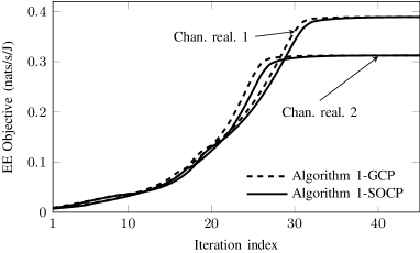
(a) Convergence over two channel realizations

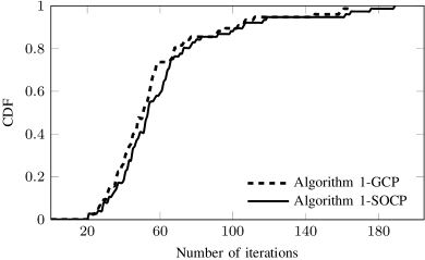
(b) CDFs of the number of required iterations to converge.

Fig. 2: Impact of conic formulation on the convergence behavior of Algorithm 1. We take $K=2$, $L=2$ and $\bar{P}=33$ dBm.

VI-A Performances of Algorithm 1 (One-Way Relaying)

In the first set of experiments, we study the impact of conic formulation of (44) on the computational complexity of Algorithm 1. Fig. 2 shows the convergence behavior of Algorithm 1 running with the generic convex program (GCP) and SOCP. Specifically, Fig. 2(a) plots the convergence of the objective over two channel realizations, and Fig. 2(b) shows the cumulative distribution functions (CDFs) of the required number of iterations to converge. Also, we provide the average total and per-iteration run time of the algorithm with the two formulations in Table II. We can see in the figure that with the SOCP, the algorithm converges with more iterations compared to the GCP. However, as shown in the table, the per-iteration run time of the SOCP (solver Fmincon) is much smaller than that of GCP (solver Fmincon), resulting that the total run time of the algorithm with the SOCP is ten times smaller than that with the GCP. In addition, the SOCP allows us to use the more efficient solver MOSEK. With this, the total run time significantly reduces.

Table II: Average per-iteration and total solver run time (in second) of Algorithm 1 adopting GCP and SOCP. We take $K=2$, $L=2$ and $\bar{P}=33$ dBm.

Solver		Fmincon	MOSEK
Algorithm1-GCP	Avg. per-iteration run time	49	N/A
	Avg. total run time	2.5e3
Algorithm1-SOCP	Avg. per-iteration run time	4.97	0.003
	Avg. total run time	220	0.17

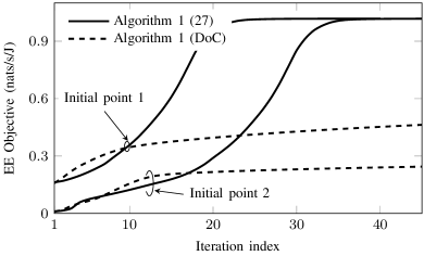
(a) Convergence over a channel realization

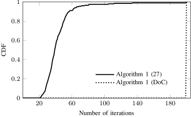
(b) CDF of the number of requirediterations to converge.

Fig. 3: Impact of approximation functions (27) and DoC on the convergence of Algorithm 1. We take $K=3$, $L=9$ and $\bar{P}=33$ dBm.

In Fig. 3, we illustrate the effectiveness of (27) in term of convergence. Particularly, Fig. 3(a) plots the convergence of Algorithm 1 using the two approximation functions, (27) and difference-of-convex (DoC) function, over a random channel realization with two different initial points generated randomly. And Fig. 3(b) shows the CDFs of number of iteration required for convergence. The results clearly demonstrate that using DoC formulations of bilinear function for the considered problems is not efficient since the corresponding iterative procedure only stops by the maximum number of iteration criteria. This confirms the use of (27).

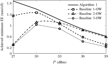
Fig. 4: Achieved EE versus the transmit power $\bar{P}$ with $K=3$ and $L=9$.

Fig. 4 depicts the averaged minimum EE performance of Algorithm 1 as a function of the maximum user power $\bar{P}$. For comparison purpose, we also provide the performance of three baseline schemes: in the first scheme, namely ‘Baseline 1-OW’, the transmit power of the users are fixed at $\bar{P}$; in the second scheme, namely ‘Baseline 2-OW’, EH time is fixed as $\tau=\frac{1}{3}$; in the third scheme, namely ‘Baseline3 -OW’, the users’ transmit power and EH time are fixed at $\bar{P}$ and $\tau=\frac{1}{3}$, respectively. For the three baseline schemes, it may happen that feasible resource allocation cannot be obtained for some channel realizations. Thus, we set the performance of those infeasible channels as zero. The first observation is that the performance of Algorithm 1 decreases when $\bar{P}$ increases. This result can be explained as follows. In an EE problem, the transmit power may be smaller than the threshold, especially when the threshold is relatively large. For this case, increasing $\bar{P}$ brings no benefit to the optimizing of the transmit power. On the other hand, as shown in (8), both $\bar{P}$ and the optimized transmit power influence the PA efficiency. And increasing $\bar{P}$ reduces the PA efficiency, leading to more amount of energy consumed at the PA as can be seen in (9). Another interesting observation is that the EEs of the three baseline schemes first increase, and then decrease as $\bar{P}$ increases. The reason is that the probabilities of infeasibility of these schemes are high when $\bar{P}$ is small. When $\bar{P}$ becomes larger, the infeasibility probabilities are smaller leading to the improved performances. When the probabilities of infeasibility are small enough, further increasing $\bar{P}$ leads to the degraded performances due to the decrease of PA efficiency. As expected, our proposed scheme outperforms the baseline ones.

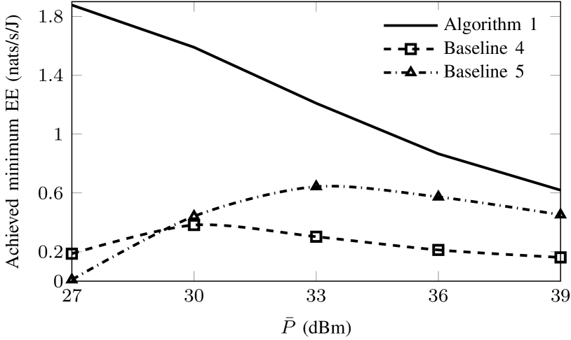
Fig. 5: Achieved minimum EE and versus the transmit power $\bar{P}$ with $K=3$ and $L=9$.

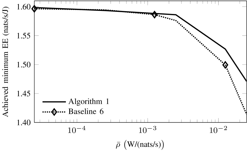
Fig. 6: Achieved minimum EE versus rate-dependent power coefficient $\bar{\rho}$ with $K=3$ and $L=9$.

In Fig. 6, we show the impacts of PA and EH models on the minimum EE performance. For this purpose, we consider the following schemes: the first scheme, named as ‘Baseline 4’, considers linear model of PA efficiency where the efficiency is fixed at 0.35. The the second scheme, named as ‘Baseline 5’, adopts the linear EH model with constant conversion efficiency 0.8. The performances of these schemes are obtained as follows. First, the design parameters are determined by suitably modifying Algorithm 1 corresponding to the considered models. From the achieved values, the minimum EE is recalculated following the PA and EH models considered in Section II. If there is infeasibility, the corresponding minimum EE is set as zero. The figure clearly shows that PA and EH models have significant influence on the performance. Similarly to Baselines 1, 2 and 3 (in Fig. 3), the performances of Baseline 4 and Baseline 5 are inferior when $\bar{P}$ is small due to high probability of infeasibility. The performance degradations of Baselines 4 and 5 are mainly because of the mismatch between the baseline schemes and the realistic models. The results again confirm the validity of our proposed scheme.

To investigate the impacts of rate-dependent signal processing power (RSPP) on the minimum EE performance, we let the rate-dependent-power coefficients in each pair be different from that of other pairs by simply setting as $\rho_{1k}^{\text{en}}=\rho_{1k}^{\text{de}}=\omega_{k}\bar{\rho}$ where $\omega_{k}=k$, and plot the performance as a function of $\bar{\rho}$ in Fig. 6. Here, the compared scheme, namely ‘Baseline 6’, takes $\rho_{ik}^{\text{en}}=\rho_{ik}^{\text{de}}=0$, and its performance is obtained similarly as that of Baseline 4 and Baseline 5 (in Fig. 6). We observe that RSPP has insignificant influence on the performance when its coefficients are small. However, when the coefficients becomes larger, the gap between Algorithm 1 and Baseline 6 is remarkable.

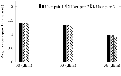
(a) Average individual EE of user pairs.

(b) CDF of Jain’s fairness index.

Fig. 7: EE fairness among the user pairs achieved by Algorithm 1 with $K=3$, and $L=12$.

Fig. 7 shows the EE fairness among user pairs versus different values of $\bar{P}$. In particular, the average individual EE of the user pairs is plotted in Fig. 7(a), and the CDFs of Jain’s fairness index [49] are shown in Fig. 7(b). It can be observed that the achieved EE is relatively balanced among all user pairs. On the other hand, the algorithm achieves absolute fairness in more than 90% of channel realizations in all considered cases of $\bar{P}$.

VI-B Performances of Algorithm 2 (Two-Way Relaying)

In Fig. 8, we evaluate the performances of Algorithm 2 in terms of convergence and minimum EE. Specifically, Fig. 8(a) plots the convergence behavior of the algorithm over a random channel realization with two different initial points also generated randomly. Compared to Algorithm 1, Algorithm 2 likely requires more iterations to converge. This can be intuitively explained by the inter-pair interference in two-way relaying systems which is more difficult to manage than that in one-way relaying systems due to the bi-directional transmission. Fig. 8(b) illustrates the average achieved minimum EE of Algorithm 2 versus the maximum transmit power $\bar{P}$. We compare Algorithm 2 with the three schemes, Baseline 1-TW, Baseline 2-TW and Baseline 3-TW which are set up similarly to Baseline 1-OW, Baseline 2-OW and Baseline 3-OW in Fig. 3. Again, we observe that the proposed scheme outperforms the others. On the other hand, for Algorithm 2, we can see that in the region of limited user power, the EE increases when $\bar{P}$ increases. This is because the effect of the gain from the additional power resource is stronger than that of the decrease because of PA efficiency. When $\bar{P}$ is large, an increase of $\bar{P}$ has insufficient influence, and thus the performance reduces with $\bar{P}$.

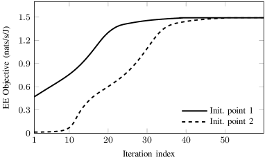
(a) Convergence of Algorithm 2 for one channel realization with $\bar{P}=33$ dBm.

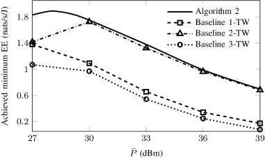
(b) Achieved minimum EE performance versus the transmit power $\bar{P}$.

Fig. 8: Performances of Algorithm 2 with $L=12$.

(a) Average individual EE of user pairs.

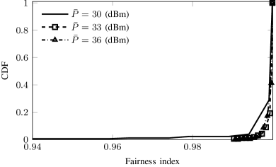
(b) CDF of Jain’s fairness index

Fig. 9: EE fairness among the user pairs achieved by Algorithm 2 with $K=3$ and $L=12$.

In Fig. 9, we plot the individual EE performances of all user pairs (Fig. 9(a)) and the CDF of fairness index (Fig. 9(b)) versus different value of $\bar{P}$. Similar to the observation in Fig. 7, the proposed EE method for two-way relaying is able to maintain the good EE fairness among all user pairs.

VI-C Performance of ZF-Based Designs

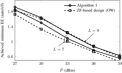
(a) Average minimum EE of Algorithm 1 and ZF-based scheme in the one-way relaying system.

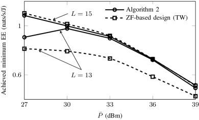
(b) Average minimum EE of Algorithm 2 and ZF-based scheme in the two-way relaying system.

Fig. 10: Average minimum EE performances versus $\bar{P}$ of Algorithms 1, 2, and ZF-based schemes.

In the following set of numerical experiments, we investigate the performances of ZF-based designs (presented in Section IV) in terms of the minimum EE and computational complexity.

Fig. 10 shows the minimum EE performances of the considered schemes. In particular, Fig. 10(a) plots the performances of Algorithm 1 and ZF-based design (OW) in the one-way relaying system, while Fig. 10(b) plots the performances of Algorithm 2 and ZF-based design (TW) in the two-way relaying system. We can observe that the performances of ZF-based schemes are inferior to Algorithms 1 and 2 when $L$ is small, and comparable, when $L$ is sufficiently large. The results are because the ZF beamforming needs a certain number of relays to form the null space.

To investigate the computational complexity of ZF-based schemes, we plot in Fig. 11 the CDFs of the required number of iterations for convergence of the considered schemes, and provide the corresponding solver running time in Table 2. It can be observed that the ZF-based schemes require smaller numbers of iterations to converge compared to Algorithms 1 and 2. In addition, the solver requires less time to solve convex subproblems in ZF-based schemes. Consequently, the total running time of the ZF-based schemes is remarkably smaller than that of Algorithms 1 and 2. Combining with the results in Fig. 10, we can conclude that, when $L$ is large, efficient solutions can be achieved with low computational cost by using the ZF-based schemes.

(a) CDF of the number of required iterations for convergence of Algorithms 1 and ZF-based scheme in one-way relaying system.

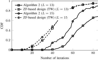
(b) CDF of the number of required iterations for convergence of Algorithms 2 and ZF-based scheme in two-way relaying system.

Fig. 11: The number of required iterations for convergence of Algorithms 1, 2, and ZF-based schemes.

Table III: Solver run time (in seconds) for Algorithms 1, 2, and the ZF-based schemes with $K=3$ and $\bar{P}=33$ dBm.

		$L=7$	$L=8$	$L=9$		$L=13$	$L=14$	$L=15$
Per-iteration run time	Algorithm 1	0.039	0.050	0.056	Algorithm 2	0.12	0.14	0.16
	ZF-based (OW)	0.019	0.028	0.037	ZF-based (TW)	0.021	0.026	0.030
Total run time	Algorithm 1	2.24	2.53	2.40	Algorithm 2	9.97	10.16	10.36
	ZF-based (OW)	0.56	0.82	1.08	ZF-based (TW)	0.96	1.16	1.28

VII Conclusion

We studied a multipair relay system where the relays harvest energy from user RF signals. We considered an energy consumption model, which accounts various realistic aspects such as rate-dependent signal processing power, dynamic power amplifier efficiency, and nonlinear EH circuits. We have investigated the problem of max-min EE fairness among user pairs by jointly designing the transmit data rate, users’ transmit power, relays’ processing coefficient, and EH time. For both one-way and two-way relaying, we have derived iterative procedures based on the IA optimization framework, where each iteration only deals with an SOCP. The proposed methods are provably convergent. In addition, for low-complexity designs, we have proposed an approach based on a combination of ZF beamforming and IA. The effectiveness of our approaches has been demonstrated by the numerical results.

-A Problem Equivalence

We justify the optimal equivalence between (43) and EEF-OW as follows. Let us denote $\bm{\psi}^{\ast}$ as the optimal solution of (43) and define $\hat{k}\triangleq\arg\max_{k\in{\cal K}}\{\hat{\eta}_{k}\}$ where $\hat{\eta}_{k}\triangleq\rho_{1k}^{\text{sp}}+\frac{P^{\prime}_{k}}{r_{1k}^{\ast}}+\frac{\tilde{\tau}^{\ast}}{r_{1k}^{\ast}}\bigl{(}\frac{\varepsilon_{1k}}{\sqrt{q_{1k}^{\ast}}}+P^{\prime\prime}_{k}\bigr{)}$. We remark that constraints in (43e) hold with equality at the optimum following the epigraph transformation. Thus it is sufficient to show that: (i) $\hat{\eta}_{\hat{k}}$ is the optimal solution of (43), i.e., $\hat{\eta}_{\hat{k}}=\eta^{\ast}$, and (ii) (34) and (6) with respect to user pair $\hat{k}$ hold with equality at the optimum. In these regards, (43) and EEF-OW obtain the same optimal values of $({\bf w}^{\ast},{\bf r}^{\ast},\tau^{\ast},{\bf p}^{\ast}$) as can be seen by constraints in (43e). Thereby, we achieve $f_{\hat{k}}^{\text{EE,OW}}(\tau^{\ast},{\bf p}^{\ast},{\bf r}^{\ast})=\Bigl{(}\rho_{1\hat{k}}^{\text{sp}}+\frac{P^{\prime}_{\hat{k}}}{r_{1\hat{k}}^{\ast}}+\frac{\tilde{\tau}^{\ast}}{r_{1\hat{k}}^{\ast}}\bigl{(}\frac{\varepsilon_{1\hat{k}}}{\sqrt{q_{1\hat{k}}^{\ast}}}+P^{\prime\prime}_{\hat{k}}\bigr{)}\Bigr{)}^{-1}=\frac{1}{\eta^{\ast}}$ which implies the equivalence between (43) and EEF-OW.

We now show (i). It is immediately seen that (40) holds at the optimum for $\hat{k}$ and $\hat{\eta}_{\hat{k}}=\eta^{\ast}$. This is because otherwise $\hat{\eta}_{\hat{k}}<\eta^{\ast}$ which means that $\eta^{\ast}$ is not the optimum. Next, we prove (ii). Let us consider problem (43) and suppose, to the contrary, that (34) does not hold at the optimum for $\hat{k}$. Then, we can scale up $r_{1\hat{k}}^{\ast}$ by a positive-scaling factor $\lambda>1$ such that $\hat{r}_{1\hat{k}}\triangleq\lambda r_{1\hat{k}}^{\ast}=\log(1+v_{1\hat{k}}^{\ast})$. And, we can easily check that new value $\hat{r}_{1k}$ is still feasible to (43). However, substituting $\hat{r}_{1k}$ to (43) results in a strictly smaller objective, i.e., $\rho_{1\hat{k}}^{\text{sp}}+\frac{P^{\prime}_{\hat{k}}}{\hat{r}_{1\hat{k}}}+\frac{\tilde{\tau}}{\hat{r}_{1\hat{k}}}\bigl{(}\frac{\varepsilon_{1\hat{k}}}{\sqrt{q_{1\hat{k}}}}+P^{\prime\prime}_{\hat{k}}\bigr{)}=\hat{\eta}_{k}<\eta^{\ast}$. This contradicts to the fact $\hat{\eta}_{k}=\eta^{\ast}$ at the optimum. Similarly, we can argue that (6) with respect to $\hat{k}$ holds with equality at the optimum of EEF-OW. This accomplishes (ii) and completes the proof.

-B Convexity of Function $x^{2}/\sqrt{y}$

We show that the function is strictly convex over $x>0,y>0$ via the second-order condition. The Hessian of the function is $\mathbf{A}=\tiny\left[\begin{array}[]{cc}2/\sqrt{y}&-x/y^{3/2}\\ -x/y^{3/2}&3x^{2}/4y^{5/2}\end{array}\right]$. Then we have

$$[v_{1}\,v_{2}]\mathbf{A}[v_{1}\,v_{2}]^{\mbox{\scriptsize T}}=\frac{2v_{1}^{2}}{\sqrt{y}}-\frac{2xv_{1}v_{2}}{y^{3/2}}+\frac{3x^{2}v_{2}^{2}}{4y^{5/2}}=\frac{2}{\sqrt{y}}(v_{1}-\frac{xv_{2}}{2y})^{2}+\frac{x^{2}v_{1}^{2}}{4y^{5/2}}>0$$

for all non-zero vector $[v_{1}\,v_{2}]$, i.e., $\mathbf{A}$ is positive definite.

It is interesting that the constraint $x^{2}/\sqrt{y}\leq t$ can be equivalently represented by two SOCs as

$$x^{2}/\sqrt{y}\leq t\Leftrightarrow\begin{cases}\|[2x,\ t-v]\|_{2}\leq t+v\\ \|[2y,\ v-1]\|_{2}\leq v+1\end{cases}.$$

References

• [1] D. Feng, C. Jiang, G. Lim, J. Cimini, L. J., G. Feng, and G. Li, “A survey of energy-efficient wireless communication,” IEEE Commun. Surveys Tuts., vol. 15, no. 1, pp. 167–178, Feb. 2013.
• [2] L. Sanguinetti, A. A. D’Amico, and Y. Rong, “A tutorial on the optimization of amplify-and-forward MIMO relay systems,” IEEE J. Sel. Areas Commun., vol. 30, no. 8, pp. 1331–1346, Sep. 2012.
• [3] 3GPP, “Overview of 3GPP Release 10 V0.2.1 (2014-06),” 3rd Generation Partnership Project, Tech. Rep. [Online]. Available: http://www.3gpp.org/specifications/releases/70-release-10
• [4] M. N. Tehrani, M. Uysal, and H. Yanikomeroglu, “Device-to-device communication in 5G cellular networks: challenges, solutions, and future directions,” IEEE Commun. Mag., vol. 52, no. 5, pp. 86–92, May 2014.
• [5] Q. Li, R. Q. Hu, Y. Qian, and G. Wu, “Cooperative communications for wireless networks: techniques and applications in LTE-advanced systems,” IEEE Wireless Commun., vol. 19, no. 2, April 2012.
• [6] B. Rankov and A. Wittneben, “Spectral efficient protocols for half-duplex fading relay channels,” IEEE J. Sel. Areas Commun., vol. 25, no. 2, pp. 379–389, Feb. 2007.
• [7] S. Fazeli-Dehkordy, S. Shahbazpanahi, and S. Gazor, “Multiple peer-to-peer communications using a network of relays,” IEEE Trans. Signal Process., vol. 57, no. 8, pp. 3053–3062, Aug. 2009.
• [8] J. Joung and A. H. Sayed, “Multiuser two-way amplify-and-forward relay processing and power control methods for beamforming systems,” IEEE Trans. Signal Process., vol. 58, no. 3, pp. 1833–1846, March 2010.
• [9] Z. Ding, W. H. Chin, and K. K. Leung, “Distributed beamforming and power allocation for cooperative networks,” IEEE Trans. Wireless Commun., vol. 7, no. 5, pp. 1817–1822, May 2008.
• [10] C. Huang, R. Zhang, and S. Cui, “Throughput maximization for the Gaussian relay channel with energy harvesting constraints,” vol. 31, no. 8, pp. 1469–1479, August 2013.
• [11] Z. Ding, S. M. Perlaza, I. Esnaola, and H. V. Poor, “Power allocation strategies in energy harvesting wireless cooperative networks,” IEEE Trans. Wireless Commun., vol. 13, no. 2, pp. 846–860, February 2014.
• [12] A. A. Nasir, X. Zhou, S. Durrani, and R. A. Kennedy, “Relaying protocols for wireless energy harvesting and information processing,” IEEE Trans. Wireless Commun., vol. 12, no. 7, pp. 3622–3636, July 2013.
• [13] X. Lu, P. Wang, D. Niyato, D. I. Kim, and Z. Han, “Wireless networks with RF energy harvesting: A contemporary survey,” IEEE Commun. Surveys Tuts., vol. 17, no. 2, pp. 757–789, Secondquarter 2015.
• [14] Ericsson White Paper, “5G energy performance,” April 2015.
• [15] A. Zappone, P. Cao, and E. A. Jorswieck, “Energy efficiency optimization in relay-assisted MIMO systems with perfect and statistical CSI,” IEEE Trans. Signal Process., vol. 62, no. 2, pp. 443–457, Jan. 2014.
• [16] F. Héliot and R. Tafazolli, “Optimal energy-efficient source and relay precoder design for cooperative MIMO-AF systems,” IEEE Trans. Signal Process., vol. 66, no. 3, pp. 573–588, Feb. 2018.
• [17] J. Zhang and M. Haardt, “Energy efficient two-way non-regenerative relaying for relays with multiple antennas,” IEEE Signal Process. Lett., vol. 22, no. 8, pp. 1079–1083, Aug. 2015.
• [18] Z. Sheng, H. D. Tuan, T. Q. Duong, and H. V. Poor, “Joint power allocation and beamforming for energy-efficient two-way multi-relay communications,” IEEE Trans. Wireless Commun., vol. 16, no. 10, pp. 6660–6671, Oct. 2017.
• [19] C. Isheden and G. P. Fettweis, “Energy-efficient multi-carrier link adaptation with sum rate-dependent circuit power,” in 2010 IEEE Global Telecommun. Conf. GLOBECOM 2010, Dec. 2010, pp. 1–6.
• [20] D. Persson, T. Eriksson, and E. G. Larsson, “Amplifier-aware multiple-input multiple-output power allocation,” IEEE Commun. Lett., vol. 17, no. 6, pp. 1112–1115, Jun. 2013.
• [21] O. Tervo, A. Tölli, M. Juntti, and L. N. Tran, “Energy-efficient beam coordination strategies with rate-dependent processing power,” IEEE Trans. Signal Process., vol. 65, no. 22, pp. 6097–6112, Nov. 2017.
• [22] O. Tervo, L. N. Tran, and M. Juntti, “Energy-efficient joint transmit beamforming and subarray selection with non-linear power amplifier efficiency,” in IEEE GlobalSIP, Dec. 2016, pp. 763–767.
• [23] Y. Cheng and M. Pesavento, “Joint optimization of source power allocation and distributed relay beamforming in multiuser peer-to-peer relay networks,” IEEE Trans. Signal Process., vol. 60, no. 6, pp. 2962–2973, June 2012.
• [24] C. Wang, H. M. Wang, D. W. K. Ng, X. G. Xia, and C. Liu, “Joint beamforming and power allocation for secrecy in peer-to-peer relay networks,” IEEE Trans. Wireless Commun., vol. 14, no. 6, pp. 3280–3293, June 2015.
• [25] M. Tao and R. Wang, “Linear precoding for multi-pair two-way MIMO relay systems with max-min fairness,” IEEE Trans. Signal Process., vol. 60, no. 10, pp. 5361–5370, Oct. 2012.
• [26] A. A. Nasir, X. Zhou, S. Durrani, and R. A. Kennedy, “Wireless-powered relays in cooperative communications: Time-switching relaying protocols and throughput analysis,” IEEE Trans. Wireless Commun., vol. 63, no. 5, pp. 1607–1622, May 2015.
• [27] Y. Huang and B. Clerckx, “Relaying strategies for wireless-powered MIMO relay networks,” IEEE Trans. Wireless Commun., vol. 15, no. 9, pp. 6033–6047, Sept. 2016.
• [28] Z. Chen, B. Xia, and H. Liu, “Wireless information and power transfer in two-way amplify-and-forward relaying channels,” in IEEE GlobalSIP, Dec 2014, pp. 168–172.
• [29] Y. Liu, “Wireless information and power transfer for multirelay-assisted cooperative communication,” IEEE Commun. Lett., vol. 20, no. 4, pp. 784–787, April 2016.
• [30] S. Salari, I. M. Kim, D. I. Kim, and F. Chan, “Joint EH time allocation and distributed beamforming in interference-limited two-way networks with EH-Based relays,” IEEE Trans. Wireless Commun., vol. 16, no. 10, pp. 6395–6408, Oct. 2017.
• [31] F. Tan, T. Lv, and S. Yang, “Power allocation optimization for energy-efficient massive MIMO aided multi-pair decode-and-forward relay systems,” vol. 65, no. 6, pp. 2368–2381, June 2017.
• [32] C. Zhang, H. Du, and J. Ge, “Energy-efficient power allocation in energy harvesting two-way AF relay systems,” IEEE Access, vol. 5, pp. 3640–3645, March 2017.
• [33] Q. Cui, Y. Zhang, W. Ni, M. Valkama, and R. Jäntti, “Energy efficiency maximization of full-duplex two-way relay with non-ideal power amplifiers and non-negligible circuit power,” IEEE Trans. Wireless Commun., vol. 16, no. 9, pp. 6264–6278, Sept. 2017.
• [34] Q. Cui, T. Yuan, and W. Ni, “Energy-efficient two-way relaying under non-ideal power amplifiers,” IEEE Trans. Veh. Technol., vol. 66, no. 2, pp. 1257–1270, Feb. 2017.
• [35] E. Boshkovska, D. W. K. Ng, N. Zlatanov, and R. Schober, “Practical non-linear energy harvesting model and resource allocation for SWIPT systems,” IEEE Commun. Lett., vol. 19, no. 12, pp. 2082–2085, Dec 2015.
• [36] Q.-D. Vu, L.-N. Tran, M. Juntti, and E.-K. Hong, “Energy-efficient bandwidth and power allocation for multi-homing networks,” IEEE Trans. Signal Process., vol. 63, no. 7, pp. 1684–1699, Apr. 2015.
• [37] A. Beck, A. Ben-Tal, and L. Tetruashvili, “A sequential parametric convex approximation method with applications to nonconvex truss topology design problem,” J. Global Optim., vol. 47, no. 1, pp. 29–51, 2010.
• [38] B. R. Marks and G. P. Wright, “A general inner approximation algorithm for nonconvex mathematical programs,” Operations Research, vol. 26, no. 4, pp. 681–683, Jul.-Aug. 1978.
• [39] S. He, Y. Huang, S. Jin, and L. Yang, “Coordinated beamforming for energy efficient transmission in multicell multiuser systems,” IEEE Trans. Commun., vol. 61, no. 12, pp. 4961–4971, Dec. 2013.
• [40] A. Zappone and E. Jorswieck, “Energy efficiency in wireless networks via fractional programming theory,” Foundations and Trends in Communications and Information Theory, vol. 11, no. 3-4, pp. 185–396, 2015.
• [41] S. Mikami, T. Takeuchi, H. Kawaguchi, C. Ohta, and M. Yoshimoto, “An efficiency degradation model of power amplifier and the impact against transmission power control for wireless sensor networks,” in 2007 IEEE Radio and Wireless Symposium,, 2007, pp. 447–450.
• [42] G. Auer, V. Giannini, C. Desset, I. Godor, P. Skillermark, M. Olsson, M. A. Imran, D. Sabella, M. J. Gonzalez, O. Blume, and A. Fehske, “How much energy is needed to run a wireless network?” IEEE Wireless Commun., vol. 18, no. 5, pp. 40–49, Oct. 2011.
• [43] T. Lipp and S. Boyd, “Variations and extension of the convex–concave procedure,” Optimization and Engineering, vol. 17, no. 2, pp. 263–287, 2016.
• [44] T. P. Dinh and H. A. L. Thi, “Recent advances in DC programming and DCA,” Transactions on Computational Intelligence XIII, vol. 8342, pp. 1–37, April 2014.
• [45] T. Dinh Quoc and M. Diehl, “Sequential Convex Programming Methods for Solving Nonlinear Optimization Problems with DC constraints,” ArXiv e-prints, Jul. 2011.
• [46] A. Ben-Tal and A. Nemirovski, Lectures on modern convex optimization.   Philadelphia: MPS-SIAM Series on Optimization, SIAM, 2001.
• [47] Q. Spencer, A. Swindlehurst, and M. Haardt, “Zero-forcing methods for downlink spatial multiplexing in multiuser MIMO channels,” IEEE Trans. Signal Process., vol. 52, no. 2, pp. 461–471, Feb 2004.
• [48] I. MOSEK ApS, 2014, [Online]. Available: www.mosek.com.
• [49] R. Jain, D.-M. Chiu, and W. R. Hawe, A quantitative measure of fairness and discrimination for resource allocation in shared computer system.   Hudson, MA: Eastern Research Laboratory, Digital Equipment Corporation, 1984.