Equation of a vacuum state and a structure formation in the universe

Abstract

The vacuum is considered as some fluid emergent from the zero-point fluctuations of the quantum fields contributing to the vacuum energy density and pressure. The equation of vacuum state and the speed of vacuum sound-waves are deduced under the assumption of zero vacuum entropy. The evolution of the background space-time metric resembles that of the Milne’s-like universe. In the framework of the five-vector theory of gravitation allowing an arbitrary choice of the energy density reference level, the dynamics of the vacuum, pressureless matter, and space-time metrics perturbations are traced under this background. The obtained results show the very early formation of the Universe structure without the need for dark matter. Thus, a vacuum can be considered as some of the dark-energy-matter unification.

1 Introduction

Clarification of the role of vacuum in the formation of the cosmic microwave background anisotropy (CMB) and the matter structures in the evolving Universe remains one of the key issues of modern cosmology despite the numerous hypotheses and suggestions [1, 2, 3, 4, 5, 6, 7]. At the same time, the application of the standard renormalization procedure [8] to gravitation seems not feasible due to the impossibility to define a vacuum state which is invariant under the general coordinate transformations [8, 5, 9]. Nevertheless, one might intuitively feel that some “pieces” of the vacuum energy density and pressure have to be omitted, while the others are to be taken into account as was demonstrated on the example of the Gowdy’s model [10]. The issue of huge vacuum energy indicates that the most diverging part of the vacuum energy density has no physical meaning and has to be discarded. Formally, this is impossible in the frameworks of the general theory of relativity (GR) because of any non-zero energy density contributes to space-time curvature. However, this procedure guaranteeing against the unphysical “piece” of the vacuum energy density can be realized within the so-called five-vector theory of gravitation (FVT) [11], in which the energy density is defined up to some constant. The remaining part of the vacuum energy can be treated as corresponding to some“fluid” possessing definite equation of state (ES).

The idea to describe a vacuum as some “fluid” defined by ES seems very tempting, starting from the concepts of a quantum “ether” [12, 13] to the models of quintessence, K-essence, and cosmological Chaplygin’s gas [14, 15, 16]. Generally speaking, the the situation looks as follows: there is no “ether” in the flat space-time owing to vacuum invariance relatively the Lorentz transformations, but in the presence of gravitation, the picture is different because there is no invariant vacuum state relatively the general coordinate transformations. As a result, one might conjecture the existence of some preferred reference frame indicating the existence of “ether” identified with a quantum vacuum.

2 Violation of gauge invariance in a framework of FVT

In GR, any spatially uniform energy density (including that of zero-point fluctuations of the quantum fields) causes the expansion of the universe. Using the Planck level of UV-cutoff results in the Planckian vacuum energy density $\rho_{vac}\sim M_{p}^{4}$ [2], which leads to the universe expanding with the Planckian rate [17]. In this sense, the vacuum energy problem is an observational fact [18]. One of the possible solutions is to build a theory of gravity, allowing an arbitrarily reference level of energy density. One such theory has long been known. That is the unimodular gravity [19, 20, 21, 22, 23, 24], which admits an arbitrary cosmological constant. However, under using of the comoving momentums cutoff, the vacuum energy density scales with time as radiation [25, 18], but not as the cosmological constant.

Recently, another theory has been suggested [11], which also leads to the Friedman equation defined up to some arbitrary constant. This constant corresponds to the invisible radiation and, thus, can compensate the vacuum energy.

Five-vector theory of gravity (FVT) [11] assumes the gauge invariance violation in GR by constraining the class of all possible metrics in varying the standard Einstein-Hilbert action. This theory arises if one varies the standard Einstein-Hilbert action over not all possible space-time metrics $g_{\mu\nu}$, but over some class of conformally-unimodular metrics [11]

$$ds^{2}\equiv g_{\mu\nu}dx^{\mu}dx^{\nu}=a^{2}\left(1-\partial_{m}P^{m}\right)^{2}d\eta^{2}-\gamma_{ij}(dx^{i}+N^{i}d\eta)(dx^{j}+N^{j}d\eta),$$ (1)

where $x^{\mu}=\{\eta,\bm{x}\}$, $\eta$ is conformal time, $\gamma_{ij}$ is a spatial metric, $a=\gamma^{1/6}$ is a locally defined scale factor, and $\gamma=\det\gamma_{ij}$. The spatial part of the interval (1) reads as

$$dl^{2}\equiv\gamma_{ij}dx^{i}dx^{j}=a^{2}(\eta,\bm{x})\tilde{\gamma}_{ij}dx^{i}dx^{j},$$ (2)

where $\tilde{\gamma}_{ij}=\gamma_{ij}/a^{2}$ is a matrix with the unit determinant.

The interval (1) is similar formally to the ADM one [26], but with the lapse function $N$ changed by the expression $1-\partial_{m}P^{m}$, where $P^{m}$ is a three-dimensional (relatively rotations) vector, and $\partial_{m}$ is a conventional particular derivative. Finaly, restrictions $\partial_{n}(\partial_{m}N^{m})=0$ and $\partial_{n}(\partial_{m}P^{m})=0$ arise because they are the Lagrange multipliers in FVT. Hamiltonian $\mathcal{H}$ and momentum $\mathcal{P}_{i}$ constraints in the gauge (1) have the same form [11] as in GR, so in FVT, and obeys the constraint constraint algebra which gives the constraint evolution equation [11]. Let us write it in the particular gauge $N=1$, $N^{i}=0$:

$$\partial_{\eta}{\mathcal{H}}=\partial_{i}\left(\tilde{\gamma}^{ij}\mathcal{P}_{j}\right),$$ (3)

$$\partial_{\eta}{\mathcal{P}_{i}}=\frac{1}{3}\partial_{i}{\mathcal{H}}.$$ (4)

One could notice that the evolution of constraints governed by (3), (4) admit adding some constant to ${\mathcal{H}}$. Thus the constraint $\mathcal{H}$ not necessarily must be zero, but $\mathcal{H}=const$ is also admitted. This fact explains why the Friedmann equation in FVT is satisfied up to some arbitrary constant. It is also interesting how black holes look in the framework of FVT [27].

3 Vacuum as a fluid

Let us consider a quantum scalar field $\hat{\phi}(\eta,\bm{x})$ against a classical background of the uniform, flat, expanding Universe with a space-time metric:

$$ds^{2}\equiv g_{\mu\nu}dx^{\mu}dx^{\nu}=a^{2}(\eta)\left(d\eta^{2}-\tilde{\gamma}_{ij}dx^{i}dx^{j}\right),$$ (5)

where $\tilde{\gamma}_{ij}=\mbox{diag}\{1,1,1\}$ is a Euclidean 3-metric. At this moment, at least one fundamental scalar field is known that is the Higgs boson [28]. Besides, as was shown in [29], the gravitational waves contribute to the vacuum energy density in the same manner as a scalar field.

The operators of the energy density and pressure of a scalar field can be written as

$$\hat{\rho}_{\phi}=\frac{1}{V}\int_{V}\left(\frac{\hat{\phi}^{\prime 2}}{2a^{2}}+\frac{(\bm{\nabla}\hat{\phi})^{2}}{2a^{2}}\right)d^{3}\bm{r},$$

$$\hat{p}_{\phi}=\frac{1}{V}\int_{V}\left(\frac{\hat{\phi}^{\prime 2}}{2a^{2}}-\frac{(\bm{\nabla}\hat{\phi})^{2}}{6a^{2}}\right)d^{3}\bm{r},$$ (6)

where $V$ is some normalizing volume which can be equaled unity. Pressure and density of all kinds of matter define the scale factor evolution of the flat Universe by the equations:

$$-\frac{1}{2}M_{p}^{2}a^{\prime 2}+\rho a^{4}=const,$$ (7)

$$M_{p}^{2}a^{\prime\prime}=(\rho-3p)a^{3},$$ (8)

where the Planck mass $M_{p}=\sqrt{\frac{3}{4\pi G}}$. In the frameworks of the FVT [30], the Friedmann equation (7) is satisfied up to some constant allowing to avoid the problem of huge vacuum energy, which diverges as fourth degree of momentum. A scalar field could be expanded over the plane wave modes $\hat{\phi}(\bm{r})=\sum_{\bm{k}}\hat{\phi}_{\bm{k}}e^{i{\bm{k}}\bm{r}},$ which are expressed through the creation and annihilation operators [8]:

$$\hat{\phi}_{\bm{k}}=\hat{\mbox{a}}^{+}_{-\bm{k}}\chi_{k}^{*}(\eta)+\hat{\mbox{a}}_{\bm{k}}\chi_{k}(\eta).$$ (9)

The complex functions $\chi_{k}(\eta)$ satisfy the relations [8]

$$\chi^{\prime\prime}_{k}+k^{2}\chi_{k}+2\frac{a^{\prime}}{a}{\chi^{\prime}}_{k}=0,$$

$$a^{2}(\eta)(\chi_{k}\,{\chi_{k}^{\prime}}^{*}-\chi_{k}^{*}\,\chi_{k}^{\prime})=i$$ (10)

and can be found in the adiabatic approximation:

$$\chi_{k}(\eta)=\frac{\exp\left({-i\int_{0}^{\eta}\sqrt{k^{2}-\frac{a^{\prime\prime}(\tau)}{a(\tau)}}\,d\tau}\right)}{\sqrt{2}a(\eta)\sqrt[4]{k^{2}-\frac{a^{\prime\prime}(\eta)}{a(\eta)}}}.$$ (11)

Let us calculate the mean vacuum energy density of a scalar field

$$\rho_{v}a^{4}=\frac{a^{2}}{2}\int\left(<0|{\hat{\phi}}^{\prime 2}|0>+<0|(\bm{\nabla}{\hat{\phi}})^{2}|0>\right)d^{3}\bm{r}=$$

$$\frac{a^{2}}{2}\sum_{\bm{k}}<0|\hat{\phi}^{\prime}_{\bm{k}}\hat{\phi}^{\prime}_{-{\bm{k}}}|0>+k^{2}<0|\hat{\phi}_{\bm{k}}\hat{\phi}_{-{\bm{k}}}|0>=\frac{a^{2}}{2}\sum_{\bm{k}}{\chi_{k}^{\prime}}^{*}\chi_{k}^{\prime}+k^{2}\chi_{k}^{*}\chi_{k}\approx$$

$$\frac{1}{2}\frac{4\pi}{(2\pi)^{3}}\left(\frac{k_{max}^{4}}{4}+\frac{k_{max}^{2}a^{\prime 2}}{4a^{2}}+O({a^{\prime}}^{3})+O(a^{\prime}a^{\prime\prime})+O(a^{\prime\prime\prime}+...)\right),~{}~{}~{}$$ (12)

where it is implied that $a^{\prime 2}$, $a^{\prime\prime}$ has the second-order of smallness, $a^{\prime 3}$, $a^{\prime\prime}a^{\prime}$ are the third-order and so on [31]. Two first terms in Eq. (12) diverge as 4th and 2nd momentum degrees, respectively. The first term can be omitted if the Friedmann equation (7) is satisfied up to some constant. In the calculation of the second term, one could use the ultra-violet cut-off $k_{max}\sim M_{p}$ at the Planck mass level [29].

One could ask why the $\bm{k}$-cutoff of comoving momentums is used instead of, for instance, a cutoff of physical momentums related to $\bm{p}=\bm{k}/a$ ($a$ is the universe scale factor)? The answer could be that it is relatively simple to construct a theory with the $\bm{k}$-cutoff, but it is challenging to introduce the $\bm{p}$-cutoff fundamentally. For instance, merely considering gravity on a lattice gives rather fundamental theory with comoving momentums restricted by the period of a lattice.

Let us for definiteness to imply that the FVT model is considered on some lattice in which the coordinate $\bm{x}$ takes discrete values. As a result, one finds for the vacuum energy density:

$$\rho_{v}=\frac{a^{\prime 2}}{2a^{6}}M_{p}^{2}S_{0},$$ (13)

where

$$S_{0}=\frac{1}{2M_{p}^{2}}\sum_{\bm{k}}\frac{1}{k}=\frac{1}{M_{p}^{2}(2\pi)^{3}}\int\frac{d^{3}\bm{k}}{2k}=\frac{k_{max}^{2}}{8\pi^{2}M_{p}^{2}}.$$

The vacuum energy density calculated is about of the critical density of $M_{p}^{2}\mathcal{H}^{2}/2$. However, as a result of an arbitrary constant on the right-hand side of Eq. (7), the concept of critical density loses its fundamental role as a demarcating line between closed and opened Universes. Here, we will consider a flat universe ad hoc.

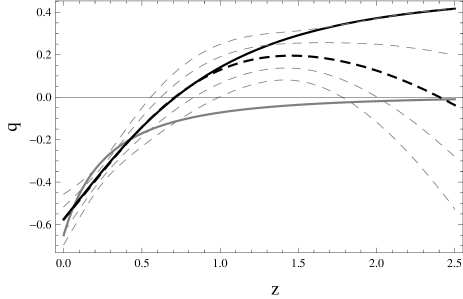
Figure 1: Deceleration parameter dependence on the redshift $z$. Solid black, gray solid and gray dashed curves correspond to the standard $\Lambda$CDM model, the vacuum domination model (20) of the present paper and the mean value of the observational data reconstruction [32], respectively. Thin dashed curves point the 1$\sigma$ and 2$\sigma$ error channels of the reconstruction.

On the way to the vacuum ES finding, the next quantity has to be calculated:

$$<0|\hat{\rho}_{\phi}-3\hat{p}_{\phi}|0>=-\frac{1}{a^{2}}\int\left(<0|{\hat{\phi}}^{\prime 2}|0>-<0|(\bm{\nabla}{\hat{\phi}})^{2}|0>\right)d^{3}\bm{r}=$$

$$-\frac{1}{a^{2}}\sum_{\bm{k}}<0|\hat{\phi}^{\prime}_{\bm{k}}\hat{\phi}^{\prime}_{-{\bm{k}}}|0>-k^{2}<0|\hat{\phi}_{\bm{k}}\hat{\phi}_{-{\bm{k}}}|0>=-\frac{1}{a^{2}}\sum_{\bm{k}}a({\chi_{k}^{\prime}}^{*}\chi_{k}^{\prime}-k^{2}\chi_{k}^{*}\chi_{k})\approx$$

$$\frac{1}{2a^{6}}\left(a{a^{\prime\prime}}-{{a^{\prime}}^{2}}\right)\sum_{\bm{k}}\frac{1}{k}+O({a^{\prime}}^{3})+O(a^{\prime}a^{\prime\prime})+O(a^{\prime\prime\prime})+...,~{}~{}~{}~{}$$ (14)

which does not contain the terms $\sim k_{max}^{4}$. The omission of items containing higher-order derivatives in (14) leads to

$$\rho_{v}-3p_{v}=\frac{1}{a^{6}}\left(a{a^{\prime\prime}}-{{a^{\prime}}^{2}}\right)M_{p}^{2}S_{0}.$$ (15)

The vacuum pressure from Eqs. (15) and (13) is:

$$p_{v}=\frac{M_{p}^{2}S_{0}}{a^{6}}\left(\frac{1}{2}a^{\prime 2}-\frac{1}{3}a^{\prime\prime}a\right).$$ (16)

It is easy to check that the vacuum energy density and pressure determined by Eqs. (13), (16) satisfy

$$\rho_{v}^{\prime}+3\frac{a^{\prime}}{a}(\rho_{v}+p_{v})=0.$$ (17)

Eq. (17) is one of the keystones describing the universe evolution. It allows considering a vacuum as some “fluid” or “substance” with the well-defined dynamical ES, which can be expressed explicitly. For this goal, one needs to find a dependence of the scale-factor $a$ on the conformal time. In a more general case, when the universe filled with a cold dust-like matter besides a vacuum, Eqs. (7), (8) take the form

$$-\frac{1}{2}M_{p}^{2}a^{\prime 2}+\rho_{v}a^{4}+\frac{1}{2}M_{p}^{2}\Omega_{m}\mathcal{H}^{2}a=const,$$ (18)

$$M_{p}^{2}a^{\prime\prime}=(\rho_{v}-3p_{v})a^{3}+\frac{1}{2}M_{p}^{2}\Omega_{m}\mathcal{H}^{2},$$ (19)

where $\Omega_{m}$ is a dimensionless constant characterizing the density of matter and $\mathcal{H}$ is a value of a of Hubble constant at the present time $\eta=\eta_{0}$, when the universe scale factor equals unity.

Figure 2: Dependencies of the vacuum ES (a) and the velocity of the scalar “sound waves” (b) on the universe scale factor. Solid line - $S_{0}=2.3$, $\Omega_{m}=0.3$, dashed line - $S_{0}=2.3$, $\Omega_{m}=0.03$.

The constant on the right hand side of Eq. (18) equals $\frac{1}{2}\mathcal{H}^{2}M_{p}^{2}(S_{0}+\Omega_{m}-1)$, to satisfy $a(\eta_{0})=1$ and $a^{\prime}(\eta_{0})=\mathcal{H}$. The resulting Hubble constant dependence on scale factor is:

$$H(a)=\frac{\dot{a}}{a}=\frac{1}{a^{2}}\frac{da}{d\eta}=\frac{\mathcal{H}}{a^{2}}\sqrt{\frac{S_{0}+\Omega_{m}-1-\Omega_{m}a}{S_{0}a^{-2}-1}},$$ (20)

where a dot denotes the differentiation on the cosmic time $dt=ad\eta$. Finally, ES reduces to

$$w_{v}=p_{v}/\rho_{v}={\left(1-\frac{2}{3}\frac{a^{\prime\prime}a}{a^{\prime 2}}\right)}=\frac{2a^{3}\Omega_{m}-3a^{2}(S_{0}+\Omega_{m}-1)+S(S_{0}+\Omega_{m}-1)}{3\left(a^{2}-S_{0}\right)((a-1)\Omega_{m}-S_{0}+1)},$$ (21)

where it is taken into account that $a^{\prime}=a^{2}H(a)$ and $a^{\prime\prime}=a^{2}H(a)\frac{d}{da}\left(a^{2}H(a)\right)$.

Eq. (21) is not singular up to the “Big Rip” (see, e.g., [33]) at $a=\sqrt{S_{0}}$, which will come in future if $S_{0}>1$. Explicit calculation of the vacuum energy density leads to

$$\rho_{v}=\frac{H^{2}M_{p}^{2}S_{0}(S_{0}+\Omega_{m}-1-a\Omega_{m})}{2a^{4}\left(S_{0}-a^{2}\right)}.$$ (22)

Let us remind that Eq. (17) leads to $\rho a^{3(1+w)}=const$ for simple dependencies of $p=w\rho$, where $w=const$. In this case, it is easy to write the Universe expansion law $a^{\prime\prime}a^{-3w}=const$ from Eq. (8). Thus, $a\sim\eta^{2+3w}$, except for $w=-1/3$ when

$$a\sim\exp\left(\mathcal{H}\eta\right).$$ (23)

The last case corresponds to the Milne’s-like Universe [34], i.e., to the exponential expansion in “conformal time” and to the linear one in “cosmic time” $dt=ad\eta$. It is necessary to remind that Milne’s Universe is spatially open, while we consider a flat Universe ad hoc.

For the vacuum ES $w\neq const$ the evolution becomes nontrivial. Eqs. (13), (16) result in the defined ES, if the expansion law is known, for example, $w_{vac}\sim 1/3$ (i.e., radiation-like) for the Milne’s-like Universe (23). However, if the vacuum has approximately the radiation-like ES at some instant of time, it does not mean that the Universe expands like the radiation dominated one. The point is that Eq. (8) for the second derivative of the Universe scale factor contains the expression $1-3w$. Thus, if $w$ is close to $1/3$ then deviations from $w=1/3$ law play role and determine the evolution. For the pure radiation-dominant Universe, these deviations are zero exactly, but for the vacuum dominated Universe they turn out substantial that leads to the Milne’s-like expansion. Actually, $H(a)\sim 1/a$ at small scale factor according to Eq. (20), i.e., as it is for the Milne’s Universe.

The results of calculation of the deceleration parameter $q(z)=-\frac{\ddot{a}}{\dot{a}^{2}}=\frac{1+z}{H}\,\frac{dH(z)}{dz}-1$ obtained from Eq. (20) are shown in Fig. 1. The Universe looks like the Milne’s one for $z\geq 2$, where the deceleration parameter is close to zero, and then comes to an acceleration phase. More general background model is discussed in [18].

Let us once more explain proximity to the Milne’s law of the Universe expansion at the simple particular case of $\Omega_{m}=0$ in which

$$\rho_{v}=\frac{H^{2}M_{p}^{2}S_{0}(S_{0}-1)}{2a^{4}\left(S_{0}-a^{2}\right)},$$ (24)

$$w_{v}=\frac{1}{3}-\frac{2a^{2}}{3(S_{0}-a^{2})}.$$ (25)

Eq. (8) leads to

$$\frac{M_{p}^{2}a^{\prime\prime}}{a}=\rho_{v}(1-3w_{v})a^{2}=\frac{\mathcal{H}^{2}M_{p}^{2}S_{0}(S_{0}-1)}{(S_{0}-a^{2})^{2}},$$ (26)

and one has $\frac{a^{\prime\prime}}{a}\sim const$ at small $a$, i.e., approximately the Milne’s-like Universe. It is instructive to compare that with the case of $w=-1/3$, $\rho=\frac{\mathcal{H}^{2}M_{p}^{2}}{2a^{2}}$ when $\frac{a^{\prime\prime}}{a}=const$, i.e., exactly the Milne’s expansion law.

Validity of Eq. (17) allows describing a vacuum as some absolutely elastic “fluid” with a “sound-speed”:

$$c_{s}^{2}=\frac{p^{\prime}}{\rho^{\prime}}=\frac{2\left(5a^{5}\Omega_{m}-a^{3}\Omega_{m}S_{0}+(7a^{2}S_{0}-9a^{4}-2S_{0}^{2})(\Omega_{m}+S_{0}-1)\right)}{3\left(a^{2}-S_{0}\right)\left(5a^{3}\Omega_{m}-3a\Omega_{m}S_{0}+(4S_{0}-6a^{2})(\Omega_{m}+S_{0}-1)\right)}.$$ (27)

According to Eqs. (12), (14), the waves of the Planck-order frequency give the main contribution to the vacuum pressure and density. These frequencies exceed the frequencies of “vacuum sound waves”. That is, the local compressions/expansions in a vacuum caused by these sound waves can be considered as the expansion and collapse of some “small universes”. Eq. (27) implies that the birth of particles from a vacuum, which would increase its entropy, is negligible. This means that an adiabatic vacuum is under consideration so that a “fluid” remains a vacuum during all the Universe evolution in the process of the scalar sound waves propagation.

Fig. 2 demonstrates that a dust-like pressureless matter has a little impact on the vacuum ES and the corresponding sound wave speed. The last increases from $1/\sqrt{3}$ up to some value at the present time. With further expansion of the Universe, the “sound speed” exceeds the speed of light and tends to infinity approximately at $a=\sqrt{\frac{2}{3}S_{0}}$. That is, Eq. (27) demonstrates that the “Big Rip” occurs earlier, than it follows from ES (21). Regarding the speed of light excess, it is difficult to say from the above empirical model whether one deals with the physical effect [35] or with a consequence of neglecting of a vacuum entropy.

Unlike the linearly expanding Universe with the ES of $w=-1/3$ [36, 37], where the imaginary sound speeds are possible, the sound speed is always positive in our case that excludes the nonphysical solutions. Such nonphysical solutions can be easily omitted in the analytical calculations [30], but they remain the issue for the numerical simulations.

4 Masses and vacuum

A massless quantum field is considered above. In the case of the massive fields, Pauli’s idea could be actual (see [25] and Refs.). That is a contribution of masses to vacuum energy from bosons and fermions should compensate each other. As a result, the main part of vacuum energy density is

$$\rho_{v}=\frac{1}{4\pi^{2}a^{4}}\int_{0}^{k_{max}}k^{2}\sqrt{k^{2}+a^{2}m^{2}}dk\approx\frac{1}{16\pi^{2}}\biggl{(}\frac{k_{max}^{4}}{a^{4}}$$

$$+\frac{m^{2}k_{max}^{2}}{a^{2}}+\frac{m^{4}}{8}\left(1+2\ln\left(\frac{m^{2}a^{2}}{4k_{max}^{2}}\right)\right)\biggr{)}.~{}~{}~{}~{}~{}~{}$$ (28)

Simultaneously, three different principles could explain why the main part of vacuum energy does not contribute to the Universe evolution. The term $k_{max}^{4}$ is omitted in the FVT gravity, where the energy reference level is arbitrary. The terms $\sim m^{4}$ are a pure mass contribution to the vacuum density. However, the condensates precipitate in the Standard Model of Electroweak Interactions to generate masses itself. A density of condensates has the same order of $m^{4}$. Overall compensation of $m^{4}-$terms including condensates should be considered. This problem stills unresolved yet, but it implies some unknown symmetry mass generating potentials in Lagrangian allowing the compensation with the accuracy at least of the order of $\sim m_{\nu}^{4}$, where $m_{\nu}$ is the neutrino mass. The only informative terms for particle physics are $\sim k_{max}^{2}m^{2}$, which gives

$$m_{H}^{2}+N_{A}m_{A}^{2}+6m_{W}^{2}+3m_{Z}^{2}=12m_{t}^{2},$$ (29)

where the top quark mass is $m_{t}=173.2~{}GeV$, the Higgs boson mass is $m_{H}=125~{}GeV$, the charged vector boson mass is $m_{W}=80,4~{}GeV$, the neutral vector boson mass is $m_{Z}=91.2~{}GeV$, and $m_{A}$ is a mass of unknown $A-$bosons contributing with the $N_{A}-$weight. Thus, the physics of vacuum beyond the Milne-like stage of the Universe expansion anticipates unknown bosons: a single boson $m_{A}\sim 530~{}Gev$, or, for instance, four bosons $m_{A}\sim 265~{}Gev$.

5 Formation of matter structures in the universe

The ES and the scalar waves speed in a vacuum found in the previous section could serve as the basis for the description of the perturbations evolution of vacuum, radiation, and matter in the expanding Universe. As was mentioned above, the Friedmann equation is satisfied up to some constant in the FVT that allows choosing an arbitrary reference level of the vacuum energy density. Briefly, the FVT theory is based on the standard Einstein-Hilbert action which is varied not over all the possible metrics, but over some restricted class of them [30]. As a result, the Hamiltonian constraint turns out to be weaker than that in GR. Perturbations of the metric of the expanding Universe looks as

Figure 3: The inhomogeneity growth factors for the different perturbation wave numbers: a,b- $k/h=0.0001~{}\mbox{Mpc}^{-1}$, c,d- $k/h=0.001~{}\mbox{Mpc}^{-1}$, e,f- $k/h=0.01~{}\mbox{Mpc}^{-1}$. Solid curves correspond to a matter, dashed curves correspond to a vacuum. $\Omega_{m}=0.3$ for (a,c,e) and $\Omega_{m}=0.03$ for (b,d,f), respectively.

$$ds^{2}=a(\eta)^{2}(1+2A)\left(d\eta^{2}-\left(\left(1+\frac{1}{3}\sum_{m=1}^{3}\partial_{m}^{2}F\right)\delta_{ij}-\partial_{i}\partial_{j}F\right)dx^{i}dx^{j}\right).$$ (30)

The metric (30) belongs to the class of metrics (1) admissible in FVT [30].

Perturbations of density, pressure and 4-velocity of every $c$-fluid are considered as $\rho_{c}(\eta,\bm{x})=\rho_{c}(\eta)+\delta\rho_{c}(\eta,\bm{x})$, $p_{c}(\eta,\bm{x})=p_{c}(\eta)+\delta p_{c}(\eta,\bm{x})$,

$$u^{\mu}_{c}=\frac{1}{a(\eta)}\{(1-A),\bm{\nabla}v_{c}(\eta,\bm{x})\},$$ (31)

where $v_{c}$ is a velocity potential. The resulting system of equations was obtained for the Fourier components of $\delta\rho_{c}(\eta,\bm{x})=\sum_{\bm{k}}\delta\rho_{c\bm{k}}(\eta)e^{i\bm{k}\bm{x}}...$

$$-6A_{\bm{k}}^{\prime}+6A_{\bm{k}}\alpha^{\prime}+k^{2}F_{\bm{k}}^{\prime}+\frac{18}{M_{p}^{2}}e^{2\alpha}\sum_{c}V_{c\bm{k}}=0,$$ (32)

$$-18\alpha^{\prime}A_{\bm{k}}^{\prime}-18A_{\bm{k}}\alpha^{\prime 2}-6k^{2}A_{\bm{k}}+k^{4}F_{\bm{k}}+\frac{18}{M_{p}^{2}}e^{2\alpha}\sum_{c}\delta\rho_{c\bm{k}}+4A_{\bm{k}}\,\rho_{c}=0,$$ (33)

$$-12A_{\bm{k}}-3\left(F_{\bm{k}}^{\prime\prime}+2\alpha^{\prime}F_{\bm{k}}^{\prime}\right)+k^{2}F_{\bm{k}}=0,$$ (34)

$$-9\left(A_{\bm{k}}^{\prime\prime}+2\alpha^{\prime}A_{\bm{k}}^{\prime}\right)-18A_{\bm{k}}\alpha^{\prime\prime}-18A_{\bm{k}}\alpha^{\prime 2}-9k^{2}A_{\bm{k}}+k^{4}F_{\bm{k}}$$

$$-\frac{9}{M_{p}^{2}}e^{2\alpha}\sum_{c}4A_{\bm{k}}(3p_{c}-\rho_{c})+3\delta p_{c\bm{k}}-\delta\rho_{c\bm{k}}=0,$$ (35)

$$-3\alpha^{\prime}(\delta p_{c\bm{k}}+\delta\rho_{c\bm{k}})-3A_{\bm{k}}^{\prime}(\rho_{c}+p_{c})-\delta\rho_{c\bm{k}}^{\prime}+k^{2}V_{c\bm{k}}=0,$$ (36)

$$(\rho_{c}+p_{c})A_{\bm{k}}+4V_{c\bm{k}}\alpha^{\prime}+\delta p_{c\bm{k}}+V_{c\bm{k}}^{\prime}=0,$$ (37)

where $V_{c}=(p_{c}+\rho_{c})v_{c}$ corresponds to every kind of a fluid.

Let us remind that “gauge invariant” potentials are usually under consideration in GR that corresponds to the metric

$$ds^{2}=a^{2}(\eta)\left((1+2\Phi(\eta,\bm{x}))d\eta^{2}-\left(1-2\Psi(\eta,\bm{x})\right)\delta_{ij}dx^{i}dx^{j}\right),$$ (38)

as well as the “gauge invariant” density contrasts and the velocity potentials:

$$\tilde{\delta}_{c\bm{k}}(\eta)=\frac{\delta\rho_{c\bm{k}}(\eta)}{\rho_{c}(\eta)}+\frac{\rho_{c}^{\prime}(\eta)}{2\rho_{c}(\eta)}F_{\bm{k}}^{\prime}(\eta),~{}~{}~{}~{}~{}\tilde{v}_{c\bm{k}}=\frac{V_{c\bm{k}}(\eta)}{\rho_{c}(\eta)+p_{c}(\eta)}-\frac{F^{\prime}_{\bm{k}}(\eta)}{2},$$

$$\Phi_{\bm{k}}(\eta)=A_{\bm{k}}(\eta)+\frac{a^{\prime}(\eta)F_{\bm{k}}^{\prime}(\eta)+a(\eta)F_{\bm{k}}^{\prime\prime}(\eta)}{2a(\eta)},$$

$$\Psi_{\bm{k}}(\eta)=-\frac{a^{\prime}(\eta)F_{\bm{k}}^{\prime}(\eta)}{2a(\eta)}-A_{\bm{k}}(\eta)+\frac{1}{6}k^{2}F_{\bm{k}}(\eta).$$ (39)

If the Friedmann equation is satisfied exactly, Eqs. (32) - (37) can be rewritten in the terms of “invariant” quantities that results in the known equations [38, 39]. However, if Friedman equation is satisfied up to only some constant, the fundamental system is (32) - (37). In this case, it is impossible to rewrite this system in the terms of invariant variables because of the metric (38) does not belong to a class of metrics regarding which the action varies in the FVT gravity [10].

Here, the authors consider a linear evolution of the inhomogeneities of pressureless matter and vacuum beyond “the last scattering surface”, when radiation decouples with the matter, and the Universe structure starts to develop [40, 41]. As is known, the anisotropy of CMB imprints the degree of spatial inhomogeneity of a baryon-photon plasma at the last scattering surface.

After decoupling, the inhomogeneities growth with the Universe evolution results in the formation of structures such as galaxies, clusters, and superclusters ($D_{k}\geq 10^{10},10^{7}$, and $10^{4}$, respectively, [42]. Let’s calculate the inhomogeneity growth factor (the “density contrast” factor):

$$D_{k}(z)=\tilde{\delta}_{k}(z)/\tilde{\delta}_{k}(1100),$$ (40)

where $z=1100$ is the redshift corresponding approximately to the last scattering surface. Eq. (40) contains the “invariant” variables, i.e., the calculation is performed in the reference system (30), but one turns finally to the expressions (39) which are the reference-frame invariant.

As is seen from Fig. 3, a, b, the inhomogeneities at the extra-large scale decrease for both matter and vacuum. At the intermediate scale (Fig. 3, c, d), vacuum decouples with matter in a sense that its perturbations grows slower. The value of the growth factor suggests that the linear theory is still valid, because the typical value of inhomogeneities at the last scattering surface is estimated as $10^{-4}-10^{-5}$. Multiplying these value by the grows factor results in quantity less than unity. At smaller scales of the order of galaxy clusters shown in Fig. 3, e, f, the inhomogeneities enter into a nonlinear regime. In the standard $\Lambda$CDM model this scale is “slightly”-nonlinear ($D_{k}\leq 10^{4}-10^{5}$), but it is strongly nonlinear in our model. We conjecture that as an evidence of early and more intensive structure formation demonstrated by the modern observational data [43, 44, 45, 41].

At smaller scales one might conjecture that such vacuum clusterization would be considered as a “dark-matter halo” formation, but such nonlinear regimes are far beyond the scope of the present paper considering only linear perturbations evolution. The above calculations are performed for two values of the pressureless matter $\Omega_{m}=0.03$, as in the standard model, and $\Omega_{m}=0.3$. The last value is preferable for Milne’s-like Universe because the nucleosynthesis in linearly coasting cosmology demands this value of baryonic matter to provide necessary amount of helium [46, 47].

6 Conclusion

It is shown that the description of a vacuum as some elastic medium (“fluid”) leads to the ES with the defined speed of scalar “sound waves”. Such a representation can be considered as a basis for the precision cosmology of the Milne’s-type Universe [36, 37, 48], with expansion close to linear. Although the horizon problem is absent for such a model, the Hubble constant $\mathcal{H}$ plays a role of a typical scale for the evolution of perturbations. In particular, the perturbations with a wave number $k<\mathcal{H}$ decrease during the Universe evolution, while the perturbations with $k>\mathcal{H}$ increase. According to numerical estimations, there is no need in the dark matter for perturbations growth, because of the perturbations increase intensively at the small scales and enter into the nonlinear regime. It seems that the Milne’s viewpoint on the necessity to proceed from a “cosmological picture” and “descent” to a local theory of gravitation still could be more relevant than it usually considered. Namely one should describe the physical and cosmological properties of vacuum fluctuations first, and only then introduce lacking pieces like dark matter and energy.

Despite the active latest debates on the Milne’s-like cosmologies (“freely coasting universe”, “$R_{h}=ct$-universe,” etc.), the discourse is staying on the natural philosophy level until now. This paper aims to divert this discussion into physical context. Namely, the vacuum ES unifying the dark energy/matter and the system of equations for the perturbations evolution provides the necessary calculational paradigm for the quantitative comparison with the standard model. One has to note that the nonlinear evolution of perturbations is much more tricky for analysis because it could require the consideration of nonlinear operators evolution for the energy density of quantized fields.

References

- [1] Y. B. Zeldovich, Sov. Phys. Usp. 24, 216 (1981).
- [2] S. Weinberg, Rev. Mod. Phys. 61, 1 (1989).
- [3] V. Sahni and A. Starobinsky, Int. J. Mod. Phys. D 09, 373 (2000).
- [4] S. M. Carroll, Living Rev. Rel. , 1 (2001), arXiv:astro-ph/0004075.
- [5] T. Padmanabhan, Phys. Rep. 380, 235 (2003).
- [6] A. Chernin, Phys. Usp. 51, 253 (2008).
- [7] M. Li, X.-D. Li, S. Wang, and Y. Wang, Comm. Theor. Phys. 56, 525 (2011).
- [8] N. D. Birrell and P. C. W. Davis, Quantum Fields in Curved Space (Cambridge University Press, Cambridge, 1982).
- [9] S. V. Anischenko, S. L. Cherkas, and V. L. Kalashnikov, Nonlin. Phenom. Compl. Syst. 12, 16 (2009), arXiv:0806.1593.
- [10] S. Cherkas and V. Kalashnikov, Theor. Phys. 2, 124 (2017).
- [11] S. L. Cherkas and V. L. Kalashnikov, Proc. Natl. Acad. Sci. Belarus, Ser. Phys.-Math. 55, 83 (2019), arXiv:1609.00811.
- [12] P. A. M. Dirac, Nature 168, 906 (2051).
- [13] V. F. Zolotarev, Soviet Physics Journal 28, 51 (1985).
- [14] M. C. Bento, O. Bertolami, and A. A. Sen, Phys. Rev. D 66, 043507 (2002).
- [15] P. T. Silva and O. Bertolami, Astr. J 599, 829 (2003).
- [16] L. Amendola and S. Tsujikawa, Dark energy: Theory and Observations (Cambridge University Press, Cambridge, 2010).
- [17] S. I. Blinnikov and A. D. Dolgov, Phys. Usp. 62, 529 (2019).
- [18] B. S. Haridasu, S. L. Cherkas, and V. L. Kalashnikov, A reference level of the universe vacuum energy density and the astrophysical data, 2019, arXiv:1912.09224.
- [19] J. J. van der Bij, H. van Dam, and Y. J. Ng, Physica A 116, 307 (1982).
- [20] F. Wilczek, Phys. Rep. 104, 143 (1984).
- [21] W. G. Unruh, Phys. Rev. D 40, 1048 (1989).
- [22] E. Alvarez, Journal of High Energy Physics 2005, 002 (2005).
- [23] M. Henneaux and C. Teitelboim, Physics Letters B 222, 195 (1989).
- [24] L. Smolin, Phys. Rev. D 80, 084003 (2009).
- [25] M. Visser, Particles 1, 138 (2018), arXiv:1610.07264.
- [26] R. Arnowitt, S. Deser, and C. W. Misner, Gen. Rel. Grav. 40, 1997 (2008).
- [27] S. L. Cherkas and V. L. Kalashnikov, Eicheons instead of black holes, 2020, arXiv:2004.03947.
- [28] E. J. Copeland, Annalen. der Phys. 528, 62 (2015).
- [29] S. L. Cherkas and V. L. Kalashnikov, JCAP 01, 028 (2007), arXiv:gr-qc/0610148.
- [30] S. L. Cherkas and V. L. Kalashnikov, Plasma perturbations and cosmic microwave background anisotropy in the linearly expanding Milne-like universe, in Fractional Dynamics, Anomalous Transport and Plasma Science, edited by C. H. Skiadas, chap. 9, Springer, Cham, 2018.
- [31] S. L. Cherkas and V. L. Kalashnikov, Universe driven by the vacuum of scalar field: VFD model, in Proc. Int. conf. “Problems of Practical Cosmology”,Saint Petersburg, Russia, June 23 - 27, 2008, pp. 135–140, 2008, arXiv:astro-ph/0611795.
- [32] B. S. Haridasu, V. V. Lukovic, M. Moresco, and N. Vittorio, JCAP 2018, 015 (2018).
- [33] G. F. R. Ellis, R. Maartens, and M. A. H. MacCallum, Relativistic Cosmology (Cambridge University Press, Cambridge, 2012).
- [34] E. A. Milne, Relativity, Gravitation and World-Structure (The Clarendon Press, Oxford, 1935).
- [35] G. F. R. Ellis, R. Maartens, and M. A. H. MacCallum, Gen. Rel. Grav. 39, 1651 (2007).
- [36] M. V. John and K. B. Joseph, Phys. Lett. B 387, 466 (1996), arXiv:gr-qc/0312040.
- [37] F. Melia, MNRAS 446, 1191 (2015).
- [38] S. Dodelson, Modern Cosmology (Elsevier, Amsterdam, 2003).
- [39] V. Mukhanov, Physical Foundations of Cosmology (Cambridge University Press, Cambridge, 2005).
- [40] V. N. Lukash and E. V. Mikheeva, Physical Cosmology (Fizmatlit, Moscow, 2010).
- [41] S. I. Blinnikov and A. D. Dolgov, Phys. Usp. 62, 529 (2019).
- [42] M. S. Longair, Galaxy Formation (Springer, Berlin, 2008).
- [43] F. Melia, Astr. J. 147, 120 (2014).
- [44] P. A. Oesch et al., Astr. J. 819, 129 (2016).
- [45] D. Waters et al., MNRAS: Letters 461, L51 (2016).
- [46] G. F. Lewis, L. Barnes, and K. R., MNRAS 460, 291 (2016).
- [47] G. Singh and D. Lohiya, MNRAS 473, 14 (2017).
- [48] A. Dev, M. Safonova, D. Jain, and D. Lohiya, Phys. Lett. B 548, 12 (2002), arXiv:astro-ph/0204150.