Variational Schemes and Geometric Simulations for a Hydrodynamic-Electrodynamic Model of Surface Plasmon Polaritons

Abstract

A class of variational schemes for the hydrodynamic-electrodynamic model of lossless free electron gas in a quasi-neutral background is developed for high-quality simulations of surface plasmon polaritons. The Lagrangian density of lossless free electron gas with a self-consistent electromagnetic field is established, and the dynamical equations with the associated constraints are obtained via a variational principle. Based on discrete exterior calculus, the action functional of this system is discretized and minimized to obtain the discrete dynamics. Newton-Raphson iteration and the biconjugate gradient stabilized method are equipped as a hybrid nonlinear-linear algebraic solver. Instead of discretizing the partial differential equations, the variational schemes have better numerical properties in secular simulations, as they preserve the discrete Lagrangian symplectic structure, gauge symmetry, and general energy-momentum density. Two numerical experiments were performed. The numerical results reproduce characteristic dispersion relations of bulk plasmons and surface plasmon polaritons, and the numerical errors of conserved quantities in all experiments are bounded by a small value after long term simulations.

PACS number(s)

73.20.Mf, 11.10.Ef, 45.20.Jj, 02.40.Yy, 03.50.-z

I Introduction

In the past two decades, there have been impressive developments and significant advancement in applications of Surface Plasmon Polaritons (SPPs), bringing many new ideas into traditional electromagnetics and optics, such as the lithography beyond the diffraction limit, chip-scale photonic circuits, plasmonic metasurfaces, bio-photonics, etc. Ritchie (1957); Barnes et al. (2003); Ozbay (2006); Zia and Brongersma (2007); Hendry et al. (2008); Kim et al. (2008); Atwater and Polman (2010); Boltasseva and Atwater (2011); Valev (2012); Fang et al. (2017). In the field of metal optics, plasmonics focuses on the collective motions of free electron gas in metal with self-consistent and external electromagnetic fields whose first-principle model is the classical particle-field theory Ritchie (1957); Barnes et al. (2003); Ozbay (2006). Direct applications of the first-principle model in macroscopic simulations face many obstacles, such as the nonlinearity, the multi-scale, and the huge degrees-of-freedom. As a simplification, linearized phenomenological models, e.g., the Drude-Lorentz (DL) model, are widely used to describe macroscopic plasmonic phenomena Barnes et al. (2003); Ozbay (2006). In a mesoscopic context, kinetic and hydrodynamic descriptions are basic physical models of plasmonics, which involve both the dynamics of free electron gas and an electromagnetic field. Therefore, high-quality numerical schemes and simulations based on the hydrodynamic model are necessary in plasmonic research.

The physics of SPPs can be described by the free electron gas model whose dynamical equations are hydrodynamic and Maxwell’s equations Ritchie (1957). For Maxwell’s equations, many numerical schemes, such as the Finite-Difference Time-Domain (FDTD) method, the Finite Element (FE) method, and the Method of Moments (MoM) have been developed, that are widely used in modern electromagnetic engineering, Radio Frequency (RF) and microwave engineering, terahertz engineering, optical engineering, metamaterial design, accelerator design, fusion engineering, radio astrophysics, geophysics, and even biomedicine Yee (1966); Harrington (1968); Taflove and Brodwin (1975); Taflove (1995). For the hydrodynamic equations, there are also many well-designed numerical schemes. In addition to the Finite Difference (FD) method and the FE method, the Finite Volume (FV) method for conservation-type equations is very popular in Computational Fluid Dynamics (CFD), which is expected to achieve superior conservations, e.g. total energy conservation Jr. J. D. Anderson (1995). Because of their nature and the advantages in their respective fields, traditional numerical methods are often extended and reformed to simulate more complicated or hybrid systems Fang et al. (2017); Chen and Chen (2012). When it comes to plasmonic phenomena, the simplest numerical treatment is introducing the DL model, which is a local linear response of the hydrodynamic equations into the FDTD or FE methods Barnes et al. (2003); Ozbay (2006). This numerical model can be conveniently solved by circular convolution or Auxiliary Differential Equation (ADE) techniques Fang et al. (2017). This linearized dispersion model provides us with abundant information about plasmonic perturbations, such as the linear dispersion relations and polarization modes, but the important nonlinear and dynamical properties, such as mode mixing, High Harmonic Generation (HHG), and the Kerr effect, are ignored Kim et al. (2008); Valev (2012). An FDTD-type method for Hydrodynamic-Maxwell equations of plasmonic metasurfaces can also be found, and many interesting results about the nonlinear effect are shown in the simulations Fang et al. (2017). Previous work showed that plasmonic phenomena are attractive and important, which means that further numerical research is necessary. As a basic tool for computational plasmonics, more advanced numerical schemes for the free electron gas model are needed.

Because of the nonlinearity and the multi-scale nature of the Hydrodynamic-Maxwell equations, high-quality simulations of SPPs face challenges. For example, numerical errors involving the momentum and energy of the electron gas and the electromagnetic field can coherently accumulate, though these errors may be small in each numerical step. The breakdown of conservation laws over a long simulation time amounts to pseudo physics. It is desirable, therefore, to use numerical integrators with good global conservative properties. The canonical symplectic integrators for Hamiltonian systems with a canonical structure first developed by K. Feng et. al. are known as a class of structure-preserving geometric algorithms that have excellent numerical performance in long-term simulations Feng (1985); Feng and Qin (2010); Benettin and Giorgilli (1994); Reich (1999); Hairer et al. (2002); Wu et al. (2003); Hairer (2005); Chin (2009); Qin et al. (2016); Tao (2016); Morrison (2017); Chen et al. (2017). Unfortunately, the hydrodynamic system does not possess a simple canonical structure, which means the canonical symplectic integrators do not apply directly Morrison (1998). As an alternative method, J. Marsden and M. West developed the variational integrator based on the discrete Hamiltonian principle for Lagrangian systems Marsden and West (2001); Lew et al. (2004); West (2004). The discrete variational principle preserves the Lagrangian structures of dynamical systems in Lagrangian form. As a significant advantage, the numerical errors of conserved quantities are bounded by a small value over a long time. The variational integrator has been widely used in many complex systems, especially in geophysics and plasma physics Qin and Guan (2008); Li et al. (2011); Squire et al. (2012a, b); Xiao et al. (2013); Zhang et al. (2014); Stamm and Shadwick (2014); Shadwick et al. (2014); Xiao et al. (2015); Kraus et al. (2017); Shi et al. (2018).

In this work, we construct a class of variational schemes for geometric simulations of SPPs, and we show the advantages of the algorithms via several numerical experiments. In Sec.II, the Lagrangian density of lossless free electron gas with a self-consistent electromagnetic field is established, and the dynamics with constraints are obtained via the variational principle. With an appropriate derivation, the standard Hydrodynamic-Maxwell equations are obtained in an arbitrary gauge. In Sec.III, the action functional is discretized via Discrete Exterior Calculus (DEC) and minimized to obtain discrete dynamics. Equipped with efficient nonlinear and linear algebraic solvers, i.e., Newton-Raphson (N-R) iteration and the Biconjugate-Gradient-Stabilized (BICGSTAB) method, the discrete system is solvable. In App.A, the detailed Jacobian of nonlinear equations is derived, which guides the procedures of nonlinear iteration and associated linear updating. In Sec.IV, the schemes are implemented to simulate bulk plasmons and SPPs. The numerical results reproduce the characteristic dispersion relations of the plasmonic systems, and they exhibit good long-term stability. These desirable features make the algorithm a powerful tool in the study of SPPs using the hydrodynamic-electrodynamic model.

II Model and Theory

II.1 Plasmonics

SPPs are a type of infrared or visible electromagnetic surface waves that travel along a metal-dielectric interface. The polariton means the wave consists of electron collective motion and a self-consistent electromagnetic field between the metal and the dielectric Barnes et al. (2003); Ozbay (2006). The simplest SPP configuration is shown in Fig.1, where a Transverse Magnetic (TM) mode propagates along an infinite interface between the metal (lower half-space) and the dielectric (upper half-space).

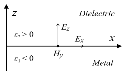
Figure 1: SPPs configuration at an infinite metal-dielectric interface.

We assume that the media are nonmagnetic. At the region where the electromagnetic wave frequency $\omega$ is lower than the metal plasma frequency $\omega_{p}$, the metallic permittivity $\epsilon_{1}<0$ and the dielectric permittivity $\epsilon_{2}>0$. Then we can write the linearized SPPs field by using the Ampère-Maxwell equation as,

$$H_{y}\left(z\right) = \tilde{H}_{1}e^{ik_{x}x}e^{k_{z1}z},$$ (1)

$$E_{x}\left(z\right) = -i\tilde{H}_{1}\frac{k_{z1}}{\omega\epsilon_{0}\epsilon_{1}}e^{ik_{x}x}e^{k_{z1}z},$$ (2)

$$E_{z}\left(z\right) = -\tilde{H}_{1}\frac{k_{x}}{\omega\epsilon_{0}\epsilon_{1}}e^{ik_{x}x}e^{k_{z1}z},$$ (3)

for the metal region, and

$$H_{y}\left(z\right) = \tilde{H}_{2}e^{ik_{x}x}e^{-k_{z2}z},$$ (4)

$$E_{x}\left(z\right) = i\tilde{H}_{2}\frac{k_{z2}}{\omega\epsilon_{0}\epsilon_{2}}e^{ik_{x}x}e^{-k_{z2}z},$$ (5)

$$E_{z}\left(z\right) = -\tilde{H}_{2}\frac{k_{x}}{\omega\epsilon_{0}\epsilon_{2}}e^{ik_{x}x}e^{-k_{z2}z},$$ (6)

for the dielectric region, where $\epsilon_{0}$ is the vacuum permittivity, and $\tilde{H}_{1}$ and $\tilde{H}_{2}$ are the magnetic field amplitudes. Applying the interface conditions $E_{x1}(0)=E_{x2}(0)$ and $H_{y1}(0)=H_{y2}(0)$ into Eqs. (1)-(6), we can obtain $\tilde{H}_{1}=\tilde{H}_{2}$ and $\epsilon_{1}k_{z2}=-\epsilon_{2}k_{z1}$. Then the linearized SPPs dispersion relations are given by using Faraday’s equation as Barnes et al. (2003),

$$k^{2}_{z1} = k^{2}_{x}-k^{2}_{0}\epsilon_{1},$$ (7)

$$k^{2}_{z2} = k^{2}_{x}-k^{2}_{0}\epsilon_{2},$$ (8)

$$k_{x} = k_{0}\sqrt{\frac{\epsilon_{1}\epsilon_{2}}{\epsilon_{1}+\epsilon_{2}}},$$ (9)

where $k_{0}=\omega/c$ is the vacuum wave number.

The previous descriptions for SPPs provide us with a basic physical image and important spectral information. At the low-frequency (terahertz or millimeter) region, Eq. (9) reduces to $k_{x}\approx{k_{0}}$ and the dielectric confinement strength $k_{z2}$ has a very small value, which means that the SPPs reduce to weak-bound Sommerfeld-Zenneck (SZ) waves. At the high-frequency (visible and near infrared) region, Eq. (9) reduces to $\omega\approx{\omega_{sp}}=\omega_{p}/\sqrt{1+\epsilon_{2}}$, where $\omega_{sp}$ is the Surface Plasmon Resonance (SPR) frequency. This means that the SPPs at the resonance region are far from the light cone, which has infinitesimal group velocity $v_{g}$ and phase velocity $v_{p}$. Both the dielectric and metal confinement strengths $k_{z2,1}$ of these quasi-static modes near the resonance region have very large values, which means the SPPs energy is strongly localized. As the cornerstone of many plasmonic techniques, the strong-bound sub-wave-length field is an important feature of the SPPs.

II.2 Lagrangian Form of Lossless Free Electron Gas

The Lagrangian density of lossless free electron gas in a quasi-neutral background with a self-consistent electromagnetic field can be defined from the hydrodynamic form as Newcomb (1962); Sahraoui et al. (2003),

$$\mathcal{L} = \mathcal{L}_{\rm{EG}}+\mathcal{L}_{\rm{EM}}+\mathcal{L}_{\rm{Int}},$$ (10)

$$\mathcal{L}_{\rm{EG}} = \frac{1}{2}mn\bm{v}^{2}+\alpha\left[\frac{\partial}{\partial{t}}n+\bigtriangledown\cdot\left(n\bm{v}\right)\right]-\lambda\left(\frac{\partial}{\partial{t}}\mu+\bm{v}\cdot\bigtriangledown\mu\right),$$ (11)

$$\mathcal{L}_{\rm{EM}} = \frac{\epsilon_{0}}{2}\left(-\bigtriangledown\phi-\frac{\partial}{\partial{t}}\bm{A}\right)^{2}-\frac{1}{2\mu_{0}}(\bigtriangledown\times\bm{A})^{2},$$ (12)

$$\mathcal{L}_{\rm{Int}} = en\bm{v}\cdot\bm{A}-e\left(n-n_{0}\right)\phi,$$ (13)

where the subscripts denote Electron Gas (EG), ElectroMagnetic (EM), and Interaction (Int), respectively. $n$ is the electron density, $n_{0}$ is the background particle density, $\bm{v}$ is the electron gas velocity, $e$ is the electron charge and $m$ is the electron mass. The electromagnetic field components $(\phi,\bm{A})$ are defined in an arbitrary gauge. This Lagrangian density is given in constraint form, where the scalar fields $\alpha$ and $\lambda$ are Lagrangian multipliers. In the last term of Eq. (10), Lin’s constraint factor $\mu$ is used to establish a complete description for the velocity and helicity Newcomb (1962); Sahraoui et al. (2003).

With the Lagrangian density (10), we can construct the action functional $S=\int_{T}\int_{\Omega}\mathcal{L}{\rm{d}}x^{3}{\rm{d}}t$ which involves the physics of lossless free electron gas. With tedious variational calculation, the total variation of $S$ with fixed boundary can be given as,

$$\delta{S} = \int_{T}\int_{\Omega}\left\{\left(\frac{1}{2}m\bm{v}^{2}+e\bm{v}\cdot\bm{A}-e\phi-\frac{\partial}{\partial{t}}\alpha-\bm{v}\cdot\bigtriangledown\alpha\right)\delta{n}\right.$$ (14)

$$+\left(mn\bm{v}+en\bm{A}-n\bigtriangledown\alpha-\lambda\bigtriangledown\mu\right)\cdot\delta\bm{v}$$

$$+\left[en\bm{v}-\epsilon_{0}\left(\bigtriangledown\frac{\partial}{\partial{t}}\phi+\frac{\partial^{2}}{\partial{t}^{2}}\bm{A}\right)-\frac{1}{\mu_{0}}\bigtriangledown\times\bigtriangledown\times\bm{A}\right]\cdot\delta\bm{A}$$

$$-\left[e\left(n-n_{0}\right)-\epsilon_{0}\left(\bigtriangledown^{2}\phi+\bigtriangledown\cdot\frac{\partial}{\partial{t}}\bm{A}\right)\right]\delta\phi$$

$$+\left[\frac{\partial}{\partial{t}}n+\bigtriangledown\cdot\left(n\bm{v}\right)\right]\delta\alpha-\left(\frac{\partial}{\partial{t}}\mu+\bm{v}\cdot\bigtriangledown\mu\right)\delta\lambda$$

$$\left.+\left[\frac{\partial}{\partial{t}}\lambda+\bigtriangledown\cdot\left(\lambda\bm{v}\right)\right]\delta\mu\right\}{\rm{d}}x^{3}{\rm{d}}t.$$

Taking variational derivative of the action functional $S$ with respect to the fields $q=(n,\bm{v},\bm{A},\phi,\alpha,\lambda,\mu)$ and minimizing $S$ by leading variational derivatives equal to 0, we can obtain the Euler-Lagrange equations of lossless free electron gas,

$$\frac{\delta{S}}{\delta{n}}=0\Rightarrow$$

$$\frac{\partial}{\partial{t}}\alpha=\frac{1}{2}m\bm{v}^{2}-\bm{v}\cdot\bigtriangledown\alpha+e\bm{v}\cdot\bm{A}-e\phi,$$ (15)

$$\frac{\delta{S}}{\delta{\bm{v}}}=0\Rightarrow$$

$$mn\bm{v}+en\bm{A}=n\bigtriangledown\alpha+\lambda\bigtriangledown\mu,$$ (16)

$$\frac{\delta{S}}{\delta{\bm{A}}}=0\Rightarrow$$

$$\frac{\partial^{2}}{\partial{t}^{2}}\bm{A}=-\frac{1}{\epsilon_{0}\mu_{0}}\bigtriangledown\times\bigtriangledown\times\bm{A}-\bigtriangledown\frac{\partial}{\partial{t}}\phi+\frac{e}{\epsilon_{0}}n\bm{v},$$ (17)

$$\frac{\delta{S}}{\delta\phi}=0\Rightarrow$$

$$\bigtriangledown^{2}\phi+\bigtriangledown\cdot\frac{\partial}{\partial{t}}\bm{A}=-\frac{e}{\epsilon_{0}}\left(n-n_{0}\right),$$ (18)

$$\frac{\delta{S}}{\delta\alpha}=0\Rightarrow$$

$$\frac{\partial}{\partial{t}}n=-\bigtriangledown\cdot\left(n\bm{v}\right),$$ (19)

$$\frac{\delta{S}}{\delta\lambda}=0\Rightarrow$$

$$\frac{\partial}{\partial{t}}\mu=-\bm{v}\cdot\bigtriangledown\mu,$$ (20)

$$\frac{\delta{S}}{\delta\mu}=0\Rightarrow$$

$$\frac{\partial}{\partial{t}}\lambda=-\bigtriangledown\cdot\left(\lambda\bm{v}\right).$$ (21)

Eqs. (15) and (21) are Lagrangian multiplier equations. Eq. (16) defines the canonical momentum density of free electron gas. Eqs. (17) and (18) are Maxwell’s equations. Eq. (19) is the continuity equation of free electron gas. Eq. (20) defines the dynamics of Lin’s constraint field. These equations provide us with a complete model to describe plasmonic phenomena.

II.3 Hydrodynamic-Maxwell Model

The Euler-Lagrange equations (15)-(21) can be recognized as a general form of the well-known hydrodynamic-Maxwell equations. Here we give a detailed derivation to illustrate the relation between two kinds of equations.

Adopting the temporal gauge $\phi=0$ explicitly, we can define the electromagnetic field components as $\bm{E}=-\partial\bm{A}/\partial{t}$ and $\mu_{0}\bm{H}=\bigtriangledown\times\bm{A}$. Taking the derivative of Eq. (16) with respect to $t$, we obtain,

$$m\left(\frac{\partial}{\partial{t}}n\right)\bm{v}+mn\frac{\partial}{\partial{t}}\bm{v}+e\left(\frac{\partial}{\partial{t}}n\right)\bm{A}+en\frac{\partial}{\partial{t}}\bm{A}$$

$$=\left(\frac{\partial}{\partial{t}}n\right)\bigtriangledown\alpha+n\bigtriangledown\frac{\partial}{\partial{t}}\alpha+\left(\frac{\partial}{\partial{t}}\lambda\right)\bigtriangledown\mu+\lambda\bigtriangledown\frac{\partial}{\partial{t}}\mu.$$ (22)

With tedious algebraic calculation, we obtain the momentum equation of free electron gas by substituting Eqs. (15) and (19)-(21) into Eq. (22) as,

$$mn\frac{\partial}{\partial{t}}\bm{v} = \left(mn\bm{v}+en\bm{A}-n\bigtriangledown\alpha-\lambda\bigtriangledown\mu\right)\cdot\bigtriangledown\bm{v}$$ (23)

$$+\left(mn\bm{v}+en\bm{A}-n\bigtriangledown\alpha-\lambda\bigtriangledown\mu\right)\times\bigtriangledown\times\bm{v}$$

$$+\bm{v}\cdot\left(\frac{\lambda}{n}\bigtriangledown{n}\bigtriangledown\mu-\bigtriangledown\lambda\bigtriangledown\mu-\lambda\bigtriangledown\bigtriangledown\mu-n\bigtriangledown\bigtriangledown\alpha+en\bigtriangledown\bm{A}\right)$$

$$+en\left[-\frac{\partial}{\partial{t}}\bm{A}+\bm{v}\times\left(\bigtriangledown\times\bm{A}\right)\right].$$

Then taking the gradient $\bigtriangledown$ on Eq. (16), we obtain,

$$-mn\bigtriangledown\bm{v} = en\bigtriangledown\bm{A}-\bigtriangledown\lambda\bigtriangledown\mu+\frac{\lambda}{n}\bigtriangledown{n}\bigtriangledown\mu-\lambda\bigtriangledown\bigtriangledown\mu-n\bigtriangledown\bigtriangledown\alpha.$$ (24)

At last, we obtain the velocity equation of free electron gas by substituting Eqs. (16) and (24) into Eq. (23) as,

$$\frac{\partial}{\partial{t}}\bm{v}=-\bm{v}\cdot\bigtriangledown\bm{v}+\frac{e}{m}\left[-\frac{\partial}{\partial{t}}\bm{A}+\bm{v}\times\left(\bigtriangledown\times\bm{A}\right)\right].$$ (25)

Based on the previous derivation, Eqs. (17)-(19) and (25) make up the standard hydrodynamic-Maxwell equations, which can be rewritten in a compact form as,

$$\frac{\partial}{\partial{t}}n+\bigtriangledown\cdot\left(n\bm{v}\right)=0,$$ (26)

$$\frac{\partial}{\partial{t}}\bm{v}+\bm{v}\cdot\bigtriangledown\bm{v}=\frac{e}{m}\left(\bm{E}+\mu_{0}\bm{v}\times\bm{H}\right),$$ (27)

$$\frac{1}{c^{2}}\frac{\partial^{2}}{\partial{t}^{2}}\bm{A}+\bigtriangledown\times\bigtriangledown\times\bm{A}=\mu_{0}en\bm{v},$$ (28)

$$\bigtriangledown\cdot\frac{\partial}{\partial{t}}\bm{A}=-\frac{e}{\epsilon_{0}}\left(n-n_{0}\right).$$ (29)

The hydrodynamic-Maxwell equations (26)-(29) are complete and self-consistent. The electromagnetic field components enter the hydrodynamic velocity equation (27) via Lorentz force. The hydrodynamic fields enter Maxwell’s equations (28)-(29) via the current and charge densities. In these equations, both the dynamics of electron collective motion and self-consistent field are involved. Based on previous discussion, both the hydrodynamic-Maxwell equations (26)-(29) and Euler-Lagrange equations (15)-(21) of lossless free electron gas can be used as the basic physical model of plasmonics.

III Numerical Strategies

III.1 DEC Based Discretization

The traditional numerical methods for an infinite dimensional dynamical system focus on the solving techniques for relevant differential or integral equations, such as the FDTD, FEM or FV types of numerical schemes for the hydrodynamic-Maxwell equations (26)-(29) or even the alternative Eqs. (15)-(21) in plasmonic research. Here we construct a numerical strategy for hydrodynamic-electrodynamic model based plasmonic phenomena simulations in a different way. Instead of directly discretizing the previous differential equations, we reconstruct the discrete dynamics via discrete variational principle, which is an infinite dimensional Hamilton’s principle analog on discrete space-time manifold. These variational schemes have particular advantages in high-quality long term simulations, as they can preserve the discrete Lagrangian symplectic structure, gauge symmetry and general energy-momentum density, which will be discussed in detail in the following sections.

The first step in numerical simulation is discretization. As a differential geometry based numerical framework, DEC defines complete operational rules on a discrete differential manifold, which form a cochain complex Kraus et al. (2017); Hirani (2003); Hiptmair (2001); Arnold et al. (2006, 2010); Holst and Stern (2012). To solve the continuous system numerically, the space-time manifold is discretized using a rectangular lattice (other lattices are also viable). Then the scalar fields, which are 3-forms, i.e. $ndx{\wedge}dy{\wedge}dz$ and ${\lambda}dx{\wedge}dy{\wedge}dz$, naturally live on the volume center of the discrete spacelike submanifold,

$$n^{n}_{i+\frac{1}{2},j+\frac{1}{2},k+\frac{1}{2}}:n\left(t_{n},x_{i}+\frac{\Delta{x}}{2},y_{j}+\frac{\Delta{y}}{2},z_{k}+\frac{\Delta{z}}{2}\right),$$ (30)

where $(t_{n},x_{i},y_{j},z_{k})$ is the coordinate of the lattice vertex. The velocity, multiplier, constraint and gauge 1-forms $\bm{v}=v_{i}dx^{i}$, $\alpha{dt}$, $\mu{dt}$ and $\bm{A}=A_{\nu}dx^{\nu}$ naturally live along the edges of the space-time lattice,

$$\phi^{n+\frac{1}{2}}_{i,j,k}:\phi\left(t_{n}+\frac{\Delta{t}}{2},x_{i},y_{j},z_{k}\right),$$ (31)

$$A^{n}_{xi+\frac{1}{2},j,k}:A_{x}\left(t_{n},x_{i}+\frac{\Delta{x}}{2},y_{j},z_{k}\right),$$ (32)

$$A^{n}_{yi,j+\frac{1}{2},k}:A_{y}\left(t_{n},x_{i},y_{j}+\frac{\Delta{y}}{2},z_{k}\right),$$ (33)

$$A^{n}_{zi,j,k+\frac{1}{2}}:A_{z}\left(t_{n},x_{i},y_{j},z_{k}+\frac{\Delta{z}}{2}\right).$$ (34)

In the above discretization, a half integer index indicates along which edge does the field resides. Then the 2-forms, e.g., $\bm{F}=\bm{{\rm{d}}}\bm{A}$, and the 4-forms, e.g., $\bm{F}\wedge*\bm{F}$, are defined on the faces and volume center of the space-time lattice respectively, where $\bm{{\rm{d}}}$ is the exterior derivative operator. The discretization of the spacelike submanifold is shown in Fig.2.

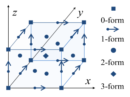
Figure 2: DEC-based discretization of the hydrodynamic-electrodynamic model in a rectangular lattice. The discrete spacelike submanifold is shown, and other types of discrete submanifolds can be given in the same way.

Based on these definitions, the exterior derivatives of discrete differential forms are naturally obtained via the forward difference operators. The exterior derivatives on the spacelike submanifold are given as,

$$\bm{{\rm{d}}}\phi=\left(\bigtriangledown\phi\right)_{i}dx^{i}=\frac{\phi_{i+1,j,k}-\phi_{i,j,k}}{\Delta{x}}dx+\frac{\phi_{i,j+1,k}-\phi_{i,j,k}}{\Delta{y}}dy+\frac{\phi_{i,j,k+1}-\phi_{i,j,k}}{\Delta{z}}dz,$$ (35)

$$\bm{{\rm{d}}}\bm{A} = \left(\bigtriangledown\times\bm{A}\right)_{i}dx^{j}{\wedge}dx^{k}$$ (36)

$$= \left(\frac{A_{zi,j+1,k+\frac{1}{2}}-A_{zi,j,k+\frac{1}{2}}}{\Delta{y}}-\frac{A_{yi,j+\frac{1}{2},k+1}-A_{yi,j+\frac{1}{2},k}}{\Delta{z}}\right)dy{\wedge}dz$$

$$+\left(\frac{A_{xi+\frac{1}{2},j,k+1}-A_{xi+\frac{1}{2},j,k}}{\Delta{z}}-\frac{A_{zi+1,j,k+\frac{1}{2}}-A_{zi,j,k+\frac{1}{2}}}{\Delta{x}}\right)dz{\wedge}dx$$

$$+\left(\frac{A_{yi+1,j+\frac{1}{2},k}-A_{yi,j+\frac{1}{2},k}}{\Delta{x}}-\frac{A_{xi+\frac{1}{2},j+1,k}-A_{xi+\frac{1}{2},j,k}}{\Delta{y}}\right)dx{\wedge}dy,$$

$$\bm{{\rm{d}}}*\bm{A}=\bigtriangledown\cdot\bm{A}dx^{i}{\wedge}dx^{j}{\wedge}dx^{k}$$

$$=\left(\frac{A_{xi+\frac{1}{2},j,k}-A_{xi-\frac{1}{2},j,k}}{\Delta{x}}+\frac{A_{yi,j+\frac{1}{2},k}-A_{yi,j-\frac{1}{2},k}}{\Delta{y}}+\frac{A_{zi,j,k+\frac{1}{2}}-A_{zi,j,k-\frac{1}{2}}}{\Delta{z}}\right)dx{\wedge}dy{\wedge}dz,$$ (37)

where $*$ is the Hodge star operator, which generates the Hodge dual form of the primary discrete form.

By using the DEC, the Lagrangian density (10) in the interval $[t_{n},t_{n+1}]$ can be discretized as,

$$\mathcal{L}^{n{\sim}n+1}_{di,j,k} = \mathcal{L}^{n{\sim}n+1}_{d{\rm{EG}}i,j,k}+\mathcal{L}^{n{\sim}n+1}_{d{\rm{EM}}i,j,k}+\mathcal{L}^{n{\sim}n+1}_{d{\rm{Int}}i,j,k},$$ (38)

$$\mathcal{L}^{n{\sim}n+1}_{d{\rm{EG}}i,j,k} = \frac{1}{2}mn^{n}_{i+\frac{1}{2},j+\frac{1}{2},k+\frac{1}{2}}\left(v^{n^{2}}_{xi+\frac{1}{2},j,k}+v^{n^{2}}_{yi,j+\frac{1}{2},k}+v^{n^{2}}_{zi,j,k+\frac{1}{2}}\right)$$ (39)

$$+\alpha^{n+\frac{1}{2}}_{i,j,k}\left(\frac{n^{n+1}_{i+\frac{1}{2},j+\frac{1}{2},k+\frac{1}{2}}-n^{n}_{i+\frac{1}{2},j+\frac{1}{2},k+\frac{1}{2}}}{\Delta{t}}\right.$$

$$+\frac{n^{n+1}_{i+\frac{1}{2},j+\frac{1}{2},k+\frac{1}{2}}v^{n+1}_{xi+\frac{1}{2},j,k}-n^{n+1}_{i-\frac{1}{2},j+\frac{1}{2},k+\frac{1}{2}}v^{n+1}_{xi-\frac{1}{2},j,k}}{\Delta{x}}$$

$$+\frac{n^{n+1}_{i+\frac{1}{2},j+\frac{1}{2},k+\frac{1}{2}}v^{n+1}_{yi,j+\frac{1}{2},k}-n^{n+1}_{i+\frac{1}{2},j-\frac{1}{2},k+\frac{1}{2}}v^{n+1}_{yi,j-\frac{1}{2},k}}{\Delta{y}}$$

$$\left.+\frac{n^{n+1}_{i+\frac{1}{2},j+\frac{1}{2},k+\frac{1}{2}}v^{n+1}_{zi,j,k+\frac{1}{2}}-n^{n+1}_{i+\frac{1}{2},j+\frac{1}{2},k-\frac{1}{2}}v^{n+1}_{zi,j,k-\frac{1}{2}}}{\Delta{z}}\right)$$

$$-\lambda^{n}_{i+\frac{1}{2},j+\frac{1}{2},k+\frac{1}{2}}\left(\frac{\mu^{n+\frac{1}{2}}_{i,j,k}-\mu^{n-\frac{1}{2}}_{i,j,k}}{\Delta{t}}+v^{n}_{xi+\frac{1}{2},j,k}\frac{\mu^{n-\frac{1}{2}}_{i+1,j,k}-\mu^{n-\frac{1}{2}}_{i,j,k}}{\Delta{x}}\right.$$

$$\left.+v^{n}_{yi,j+\frac{1}{2},k}\frac{\mu^{n-\frac{1}{2}}_{i,j+1,k}-\mu^{n-\frac{1}{2}}_{i,j,k}}{\Delta{y}}+v^{n}_{zi,j,k+\frac{1}{2}}\frac{\mu^{n-\frac{1}{2}}_{i,j,k+1}-\mu^{n-\frac{1}{2}}_{i,j,k}}{\Delta{z}}\right),$$

$$\mathcal{L}^{n{\sim}n+1}_{d{\rm{EM}}i,j,k} = \frac{\epsilon_{0}}{2}\left[\left(\frac{\phi^{n+\frac{1}{2}}_{i+1,j,k}-\phi^{n+\frac{1}{2}}_{i,j,k}}{\Delta{x}}+\frac{A^{n+1}_{xi+\frac{1}{2},j,k}-A^{n}_{xi+\frac{1}{2},j,k}}{\Delta{t}}\right)^{2}\right.$$ (40)

$$+\left(\frac{\phi^{n+\frac{1}{2}}_{i,j+1,k}-\phi^{n+\frac{1}{2}}_{i,j,k}}{\Delta{y}}+\frac{A^{n+1}_{yi,j+\frac{1}{2},k}-A^{n}_{yi,j+\frac{1}{2},k}}{\Delta{t}}\right)^{2}$$

$$\left.+\left(\frac{\phi^{n+\frac{1}{2}}_{i,j,k+1}-\phi^{n+\frac{1}{2}}_{i,j,k}}{\Delta{z}}+\frac{A^{n+1}_{zi,j,k+\frac{1}{2}}-A^{n}_{zi,j,k+\frac{1}{2}}}{\Delta{t}}\right)^{2}\right]$$

$$-\frac{1}{2\mu_{0}}\left[\left(\frac{A^{n}_{zi,j+1,k+\frac{1}{2}}-A^{n}_{zi,j,k+\frac{1}{2}}}{\Delta{y}}-\frac{A^{n}_{yi,j+\frac{1}{2},k+1}-A^{n}_{yi,j+\frac{1}{2},k}}{\Delta{z}}\right)^{2}\right.$$

$$+\left(\frac{A^{n}_{xi+\frac{1}{2},j,k+1}-A^{n}_{xi+\frac{1}{2},j,k}}{\Delta{z}}-\frac{A^{n}_{zi+1,j,k+\frac{1}{2}}-A^{n}_{zi,j,k+\frac{1}{2}}}{\Delta{x}}\right)^{2}$$

$$\left.+\left(\frac{A^{n}_{yi+1,j+\frac{1}{2},k}-A^{n}_{yi,j+\frac{1}{2},k}}{\Delta{x}}-\frac{A^{n}_{xi+\frac{1}{2},j+1,k}-A^{n}_{xi+\frac{1}{2},j,k}}{\Delta{y}}\right)^{2}\right],$$

$$\mathcal{L}^{n{\sim}n+1}_{d{\rm{Int}}i,j,k} = en^{n}_{i+\frac{1}{2},j+\frac{1}{2},k+\frac{1}{2}}\left(v^{n}_{xi+\frac{1}{2},j,k}A^{n}_{xi+\frac{1}{2},j,k}+v^{n}_{yi,j+\frac{1}{2},k}A^{n}_{yi,j+\frac{1}{2},k}+v^{n}_{zi,j,k+\frac{1}{2}}A^{n}_{zi,j,k+\frac{1}{2}}\right)$$ (41)

$$-e\left(n^{n}_{i+\frac{1}{2},j+\frac{1}{2},k+\frac{1}{2}}-n_{0}\right)\phi^{n+\frac{1}{2}}_{i,j,k}.$$

Then the action functional of discrete dynamical system is,

$$S_{d}=\sum^{N}_{n=0}L^{n{\sim}n+1}_{d}\Delta{t},$$ (42)

$$L^{n{\sim}n+1}_{d}=\sum_{i,j,k}\mathcal{L}^{n{\sim}n+1}_{di,j,k}\Delta{x}\Delta{y}\Delta{z},$$ (43)

where the functional $L^{n{\sim}n+1}_{d}$ is the Lagrangian of discrete dynamical system in interval $[t_{n},t_{n+1}]$.

III.2 Variational Schemes

With DEC-based discretization, we reconstruct a field theory on the discrete space-time manifold. Then the variational derivatives of action $S_{d}$ with respect to fields reduce to partial derivatives with respect to discrete differential forms. By minimizing the action, we obtain the discrete dynamical equations,

$$\frac{\partial{S_{d}}}{\partial{n^{n}_{i+\frac{1}{2},j+\frac{1}{2},k+\frac{1}{2}}}}=\frac{\partial(L^{n-1{\sim}n}_{d}+L^{n{\sim}n+1}_{d})}{\partial{n^{n}_{i+\frac{1}{2},j+\frac{1}{2},k+\frac{1}{2}}}}\Delta{t}=0\Rightarrow$$

$$\alpha^{n+\frac{1}{2}}_{i,j,k}-\frac{m\Delta{t}}{2}\left(v^{n^{2}}_{xi+\frac{1}{2},j,k}+v^{n^{2}}_{yi,j+\frac{1}{2},k}+v^{n^{2}}_{zi,j,k+\frac{1}{2}}\right)$$

$$-e\Delta{t}\left(v^{n}_{xi+\frac{1}{2},j,k}A^{n}_{xi+\frac{1}{2},j,k}+v^{n}_{yi,j+\frac{1}{2},k}A^{n}_{yi,j+\frac{1}{2},k}+v^{n}_{zi,j,k+\frac{1}{2}}A^{n}_{zi,j,k+\frac{1}{2}}\right)+e\Delta{t}\phi^{n+\frac{1}{2}}_{i,j,k}$$

$$+\frac{\Delta{t}}{\Delta{x}}v^{n}_{xi+\frac{1}{2},j,k}\left(\alpha^{n-\frac{1}{2}}_{i+1,j,k}-\alpha^{n-\frac{1}{2}}_{i,j,k}\right)+\frac{\Delta{t}}{\Delta{y}}v^{n}_{yi,j+\frac{1}{2},k}\left(\alpha^{n-\frac{1}{2}}_{i,j+1,k}-\alpha^{n-\frac{1}{2}}_{i,j,k}\right)$$

$$+\frac{\Delta{t}}{\Delta{z}}v^{n}_{zi,j,k+\frac{1}{2}}\left(\alpha^{n-\frac{1}{2}}_{i,j,k+1}-\alpha^{n-\frac{1}{2}}_{i,j,k}\right)=\alpha^{n-\frac{1}{2}}_{i,j,k},$$ (44)

$$\frac{\partial{S_{d}}}{\partial{v^{n}_{xi+\frac{1}{2},j,k}}}=\frac{\partial(L^{n-1{\sim}n}_{d}+L^{n{\sim}n+1}_{d})}{\partial{v^{n}_{xi+\frac{1}{2},j,k}}}\Delta{t}=0\Rightarrow$$

$$mn^{n}_{i+\frac{1}{2},j+\frac{1}{2},k+\frac{1}{2}}v^{n}_{xi+\frac{1}{2},j,k}+en^{n}_{i+\frac{1}{2},j+\frac{1}{2},k+\frac{1}{2}}A^{n}_{xi+\frac{1}{2},j,k}$$

$$=n^{n}_{i+\frac{1}{2},j+\frac{1}{2},k+\frac{1}{2}}\frac{\alpha^{n-\frac{1}{2}}_{i+1,j,k}-\alpha^{n-\frac{1}{2}}_{i,j,k}}{\Delta{x}}+\lambda^{n}_{i+\frac{1}{2},j+\frac{1}{2},k+\frac{1}{2}}\frac{\mu^{n-\frac{1}{2}}_{i+1,j,k}-\mu^{n-\frac{1}{2}}_{i,j,k}}{\Delta{x}},$$ (45)

$$\frac{\partial{S_{d}}}{\partial{v^{n}_{yi,j+\frac{1}{2},k}}}=\frac{\partial(L^{n-1{\sim}n}_{d}+L^{n{\sim}n+1}_{d})}{\partial{v^{n}_{yi,j+\frac{1}{2},k}}}\Delta{t}=0\Rightarrow$$

$$mn^{n}_{i+\frac{1}{2},j+\frac{1}{2},k+\frac{1}{2}}v^{n}_{yi,j+\frac{1}{2},k}+en^{n}_{i+\frac{1}{2},j+\frac{1}{2},k+\frac{1}{2}}A^{n}_{yi,j+\frac{1}{2},k}$$

$$=n^{n}_{i+\frac{1}{2},j+\frac{1}{2},k+\frac{1}{2}}\frac{\alpha^{n-\frac{1}{2}}_{i,j+1,k}-\alpha^{n-\frac{1}{2}}_{i,j,k}}{\Delta{y}}+\lambda^{n}_{i+\frac{1}{2},j+\frac{1}{2},k+\frac{1}{2}}\frac{\mu^{n-\frac{1}{2}}_{i,j+1,k}-\mu^{n-\frac{1}{2}}_{i,j,k}}{\Delta{y}},$$ (46)

$$\frac{\partial{S_{d}}}{\partial{v^{n}_{zi,j,k+\frac{1}{2}}}}=\frac{\partial(L^{n-1{\sim}n}_{d}+L^{n{\sim}n+1}_{d})}{\partial{v^{n}_{zi,j,k+\frac{1}{2}}}}\Delta{t}=0\Rightarrow$$

$$mn^{n}_{i+\frac{1}{2},j+\frac{1}{2},k+\frac{1}{2}}v^{n}_{zi,j,k+\frac{1}{2}}+en^{n}_{i+\frac{1}{2},j+\frac{1}{2},k+\frac{1}{2}}A^{n}_{zi,j,k+\frac{1}{2}}$$

$$=n^{n}_{i+\frac{1}{2},j+\frac{1}{2},k+\frac{1}{2}}\frac{\alpha^{n-\frac{1}{2}}_{i,j,k+1}-\alpha^{n-\frac{1}{2}}_{i,j,k}}{\Delta{z}}+\lambda^{n}_{i+\frac{1}{2},j+\frac{1}{2},k+\frac{1}{2}}\frac{\mu^{n-\frac{1}{2}}_{i,j,k+1}-\mu^{n-\frac{1}{2}}_{i,j,k}}{\Delta{z}},$$ (47)

$$\frac{\partial{S_{d}}}{\partial{A^{n}_{xi+\frac{1}{2},j,k}}}=\frac{\partial(L^{n-1{\sim}n}_{d}+L^{n{\sim}n+1}_{d})}{\partial{A^{n}_{xi+\frac{1}{2},j,k}}}\Delta{t}=0\Rightarrow$$

$$\frac{\epsilon_{0}}{\Delta{t}^{2}}A^{n+1}_{xi+\frac{1}{2},j,k}=-\frac{\epsilon_{0}}{\Delta{t}\Delta{x}}\left(\phi^{n+\frac{1}{2}}_{i+1,j,k}-\phi^{n+\frac{1}{2}}_{i,j,k}-\phi^{n-\frac{1}{2}}_{i+1,j,k}+\phi^{n-\frac{1}{2}}_{i,j,k}\right)$$

$$+\frac{A^{n}_{xi+\frac{1}{2},j,k+1}-2A^{n}_{xi+\frac{1}{2},j,k}+A^{n}_{xi+\frac{1}{2},j,k-1}}{\mu_{0}\Delta{z}^{2}}+\frac{A^{n}_{xi+\frac{1}{2},j+1,k}-2A^{n}_{xi+\frac{1}{2},j,k}+A^{n}_{xi+\frac{1}{2},j-1,k}}{\mu_{0}\Delta{y}^{2}}$$

$$-\frac{A^{n}_{zi+1,j,k+\frac{1}{2}}-A^{n}_{zi+1,j,k-\frac{1}{2}}-A^{n}_{zi,j,k+\frac{1}{2}}+A^{n}_{zi,j,k-\frac{1}{2}}}{\mu_{0}\Delta{x}\Delta{z}}$$

$$-\frac{A^{n}_{yi+1,j+\frac{1}{2},k}-A^{n}_{yi+1,j-\frac{1}{2},k}-A^{n}_{yi,j+\frac{1}{2},k}+A^{n}_{yi,j-\frac{1}{2},k}}{\mu_{0}\Delta{x}\Delta{y}}$$

$$+en^{n}_{i+\frac{1}{2},j+\frac{1}{2},k+\frac{1}{2}}v^{n}_{xi+\frac{1}{2},j,k}+\frac{2\epsilon_{0}}{\Delta{t}^{2}}A^{n}_{xi+\frac{1}{2},j,k}-\frac{\epsilon_{0}}{\Delta{t}^{2}}A^{n-1}_{xi+\frac{1}{2},j,k},$$ (48)

$$\frac{\partial{S_{d}}}{\partial{A^{n}_{yi,j+\frac{1}{2},k}}}=\frac{\partial(L^{n-1{\sim}n}_{d}+L^{n{\sim}n+1}_{d})}{\partial{A^{n}_{yi,j+\frac{1}{2},k}}}\Delta{t}=0\Rightarrow$$

$$\frac{\epsilon_{0}}{\Delta{t}^{2}}A^{n+1}_{yi,j+\frac{1}{2},k}=-\frac{\epsilon_{0}}{\Delta{t}\Delta{y}}\left(\phi^{n+\frac{1}{2}}_{i,j+1,k}-\phi^{n+\frac{1}{2}}_{i,j,k}-\phi^{n-\frac{1}{2}}_{i,j+1,k}+\phi^{n-\frac{1}{2}}_{i,j,k}\right)$$

$$+\frac{A^{n}_{yi+1,j+\frac{1}{2},k}-2A^{n}_{yi,j+\frac{1}{2},k}+A^{n}_{yi-1,j+\frac{1}{2},k}}{\mu_{0}\Delta{x}^{2}}+\frac{A^{n}_{yi,j+\frac{1}{2},k+1}-2A^{n}_{yi,j+\frac{1}{2},k}+A^{n}_{yi,j+\frac{1}{2},k-1}}{\mu_{0}\Delta{z}^{2}}$$

$$-\frac{A^{n}_{xi+\frac{1}{2},j+1,k}-A^{n}_{xi-\frac{1}{2},j+1,k}-A^{n}_{xi+\frac{1}{2},j,k}+A^{n}_{xi-\frac{1}{2},j,k}}{\mu_{0}\Delta{y}\Delta{x}}$$

$$-\frac{A^{n}_{zi,j+1,k+\frac{1}{2}}-A^{n}_{zi,j+1,k-\frac{1}{2}}-A^{n}_{zi,j,k+\frac{1}{2}}+A^{n}_{zi,j,k-\frac{1}{2}}}{\mu_{0}\Delta{y}\Delta{z}}$$

$$+en^{n}_{i+\frac{1}{2},j+\frac{1}{2},k+\frac{1}{2}}v^{n}_{yi,j+\frac{1}{2},k}+\frac{2\epsilon_{0}}{\Delta{t}^{2}}A^{n}_{yi,j+\frac{1}{2},k}-\frac{\epsilon_{0}}{\Delta{t}^{2}}A^{n-1}_{yi,j+\frac{1}{2},k},$$ (49)

$$\frac{\partial{S_{d}}}{\partial{A^{n}_{zi,j,k+\frac{1}{2}}}}=\frac{\partial(L^{n-1{\sim}n}_{d}+L^{n{\sim}n+1}_{d})}{\partial{A^{n}_{zi,j,k+\frac{1}{2}}}}=0\Rightarrow$$

$$\frac{\epsilon_{0}}{\Delta{t}^{2}}A^{n+1}_{zi,j,k+\frac{1}{2}}=-\frac{\epsilon_{0}}{\Delta{t}\Delta{z}}\left(\phi^{n+\frac{1}{2}}_{i,j,k+1}-\phi^{n+\frac{1}{2}}_{i,j,k}-\phi^{n-\frac{1}{2}}_{i,j,k+1}+\phi^{n-\frac{1}{2}}_{i,j,k}\right)$$

$$+\frac{A^{n}_{zi,j+1,k+\frac{1}{2}}-2A^{n}_{zi,j,k+\frac{1}{2}}+A^{n}_{zi,j-1,k+\frac{1}{2}}}{\mu_{0}\Delta{y}^{2}}+\frac{A^{n}_{zi+1,j,k+\frac{1}{2}}-2A^{n}_{zi,j,k+\frac{1}{2}}+A^{n}_{zi-1,j,k+\frac{1}{2}}}{\mu_{0}\Delta{x}^{2}}$$

$$-\frac{A^{n}_{yi,j+\frac{1}{2},k+1}-A^{n}_{yi,j-\frac{1}{2},k+1}-A^{n}_{yi,j+\frac{1}{2},k}+A^{n}_{yi,j-\frac{1}{2},k}}{\mu_{0}\Delta{z}\Delta{y}}$$

$$-\frac{A^{n}_{xi+\frac{1}{2},j,k+1}-A^{n}_{xi-\frac{1}{2},j,k+1}-A^{n}_{xi+\frac{1}{2},j,k}+A^{n}_{xi-\frac{1}{2},j,k}}{\mu_{0}\Delta{z}\Delta{x}}$$

$$+en^{n}_{i+\frac{1}{2},j+\frac{1}{2},k+\frac{1}{2}}v^{n}_{zi,j,k+\frac{1}{2}}+\frac{2\epsilon_{0}}{\Delta{t}^{2}}A^{n}_{zi,j,k+\frac{1}{2}}-\frac{\epsilon_{0}}{\Delta{t}^{2}}A^{n-1}_{zi,j,k+\frac{1}{2}},$$ (50)

$$\frac{\partial{S_{d}}}{\partial\phi^{n+\frac{1}{2}}_{i,j,k}}=\frac{\partial{L^{n{\sim}n+1}_{d}}}{\partial\phi^{n+\frac{1}{2}}_{i,j,k}}\Delta{t}=0\Rightarrow$$

$$\frac{\phi^{n+\frac{1}{2}}_{i+1,j,k}-2\phi^{n+\frac{1}{2}}_{i,j,k}+\phi^{n+\frac{1}{2}}_{i-1,j,k}}{\Delta{x}^{2}}+\frac{\phi^{n+\frac{1}{2}}_{i,j+1,k}-2\phi^{n+\frac{1}{2}}_{i,j,k}+\phi^{n+\frac{1}{2}}_{i,j-1,k}}{\Delta{y}^{2}}+\frac{\phi^{n+\frac{1}{2}}_{i,j,k+1}-2\phi^{n+\frac{1}{2}}_{i,j,k}+\phi^{n+\frac{1}{2}}_{i,j,k-1}}{\Delta{z}^{2}}$$

$$+\frac{A^{n+1}_{xi+\frac{1}{2},j,k}-A^{n}_{xi+\frac{1}{2},j,k}-A^{n+1}_{xi-\frac{1}{2},j,k}+A^{n}_{xi-\frac{1}{2},j,k}}{\Delta{t}\Delta{x}}$$

$$+\frac{A^{n+1}_{yi,j+\frac{1}{2},k}-A^{n}_{yi,j+\frac{1}{2},k}-A^{n+1}_{yi,j-\frac{1}{2},k}+A^{n}_{yi,j-\frac{1}{2},k}}{\Delta{t}\Delta{y}}$$

$$+\frac{A^{n+1}_{zi,j,k+\frac{1}{2}}-A^{n}_{zi,j,k+\frac{1}{2}}-A^{n+1}_{zi,j,k-\frac{1}{2}}+A^{n}_{zi,j,k-\frac{1}{2}}}{\Delta{t}\Delta{z}}=-\frac{e}{\epsilon_{0}}\left(n^{n}_{i+\frac{1}{2},j+\frac{1}{2},k+\frac{1}{2}}-n_{0}\right),$$ (51)

$$\frac{\partial{S_{d}}}{\partial\alpha^{n+\frac{1}{2}}_{i,j,k}}=\frac{\partial{L^{n{\sim}n+1}_{d}}}{\partial\alpha^{n+\frac{1}{2}}_{i,j,k}}\Delta{t}=0\Rightarrow$$

$$n^{n+1}_{i+\frac{1}{2},j+\frac{1}{2},k+\frac{1}{2}}+\frac{\Delta{t}}{\Delta{x}}\left(n^{n+1}_{i+\frac{1}{2},j+\frac{1}{2},k+\frac{1}{2}}v^{n+1}_{xi+\frac{1}{2},j,k}-n^{n+1}_{i-\frac{1}{2},j+\frac{1}{2},k+\frac{1}{2}}v^{n+1}_{xi-\frac{1}{2},j,k}\right)$$

$$+\frac{\Delta{t}}{\Delta{y}}\left(n^{n+1}_{i+\frac{1}{2},j+\frac{1}{2},k+\frac{1}{2}}v^{n+1}_{yi,j+\frac{1}{2},k}-n^{n+1}_{i+\frac{1}{2},j-\frac{1}{2},k+\frac{1}{2}}v^{n+1}_{yi,j-\frac{1}{2},k}\right)$$

$$+\frac{\Delta{t}}{\Delta{z}}\left(n^{n+1}_{i+\frac{1}{2},j+\frac{1}{2},k+\frac{1}{2}}v^{n+1}_{zi,j,k+\frac{1}{2}}-n^{n+1}_{i+\frac{1}{2},j+\frac{1}{2},k-\frac{1}{2}}v^{n+1}_{zi,j,k-\frac{1}{2}}\right)=n^{n}_{i+\frac{1}{2},j+\frac{1}{2},k+\frac{1}{2}},$$ (52)

$$\frac{\partial{S_{d}}}{\partial\lambda^{n}_{i+\frac{1}{2},j+\frac{1}{2},k+\frac{1}{2}}}=\frac{\partial{L^{n{\sim}n+1}_{d}}}{\partial\lambda^{n}_{i+\frac{1}{2},j+\frac{1}{2},k+\frac{1}{2}}}\Delta{t}=0\Rightarrow$$

$$\mu^{n+\frac{1}{2}}_{i,j,k}=\mu^{n-\frac{1}{2}}_{i,j,k}-\frac{\Delta{t}}{\Delta{x}}v^{n}_{xi+\frac{1}{2},j,k}\left(\mu^{n-\frac{1}{2}}_{i+1,j,k}-\mu^{n-\frac{1}{2}}_{i,j,k}\right)$$

$$-\frac{\Delta{t}}{\Delta{y}}v^{n}_{yi,j+\frac{1}{2},k}\left(\mu^{n-\frac{1}{2}}_{i,j+1,k}-\mu^{n-\frac{1}{2}}_{i,j,k}\right)-\frac{\Delta{t}}{\Delta{z}}v^{n}_{zi,j,k+\frac{1}{2}}\left(\mu^{n-\frac{1}{2}}_{i,j,k+1}-\mu^{n-\frac{1}{2}}_{i,j,k}\right),$$ (53)

$$\frac{\partial{S_{d}}}{\partial\mu^{n-\frac{1}{2}}_{i,j,k}}=\frac{\partial(L^{n-1{\sim}n}_{d}+L^{n{\sim}n+1}_{d})}{\partial\mu^{n-\frac{1}{2}}_{i,j,k}}\Delta{t}=0\Rightarrow$$

$$\lambda^{n}_{i+\frac{1}{2},j+\frac{1}{2},k+\frac{1}{2}}+\frac{\Delta{t}}{\Delta{x}}\left(\lambda^{n}_{i+\frac{1}{2},j+\frac{1}{2},k+\frac{1}{2}}v^{n}_{xi+\frac{1}{2},j,k}-\lambda^{n}_{i-\frac{1}{2},j+\frac{1}{2},k+\frac{1}{2}}v^{n}_{xi-\frac{1}{2},j,k}\right)$$

$$+\frac{\Delta{t}}{\Delta{y}}\left(\lambda^{n}_{i+\frac{1}{2},j+\frac{1}{2},k+\frac{1}{2}}v^{n}_{yi,j+\frac{1}{2},k}-\lambda^{n}_{i+\frac{1}{2},j-\frac{1}{2},k+\frac{1}{2}}v^{n}_{yi,j-\frac{1}{2},k}\right)$$

$$+\frac{\Delta{t}}{\Delta{z}}\left(\lambda^{n}_{i+\frac{1}{2},j+\frac{1}{2},k+\frac{1}{2}}v^{n}_{zi,j,k+\frac{1}{2}}-\lambda^{n}_{i+\frac{1}{2},j+\frac{1}{2},k-\frac{1}{2}}v^{n}_{zi,j,k-\frac{1}{2}}\right)=\lambda^{n-1}_{i+\frac{1}{2},j+\frac{1}{2},k+\frac{1}{2}}.$$ (54)

Eqs. (45)-(47) and (51) are constraints that restrict the solution manifold. Both initialization and evolution should be restricted by these numerical constraints. Eqs. (48)-(50) are explicit schemes used for updating the gauge field components. We emphasize that in a DEC framework and a rectangular lattice, the variational schemes (48)-(50) of Maxwell’s equations are equal to the traditional FDTD method. Based on DEC, the electromagnetic fields in a rectangular lattice are defined as,

$$E^{n+\frac{1}{2}}_{xi+\frac{1}{2},j,k}=-\frac{A^{n+1}_{xi+\frac{1}{2},j,k}-A^{n}_{xi+\frac{1}{2},j,k}}{\Delta{t}},$$ (55)

$$E^{n+\frac{1}{2}}_{yi,j+\frac{1}{2},k}=-\frac{A^{n+1}_{yi,j+\frac{1}{2},k}-A^{n}_{yi,j+\frac{1}{2},k}}{\Delta{t}},$$ (56)

$$E^{n+\frac{1}{2}}_{zi,j,k+\frac{1}{2}}=-\frac{A^{n+1}_{zi,j,k+\frac{1}{2}}-A^{n}_{zi,j,k+\frac{1}{2}}}{\Delta{t}},$$ (57)

$$\mu_{0}H^{n}_{xi,j+\frac{1}{2},k+\frac{1}{2}}=\frac{A^{n}_{zi,j+1,k+\frac{1}{2}}-A^{n}_{zi,j,k+\frac{1}{2}}}{\Delta{y}}-\frac{A^{n}_{yi,j+\frac{1}{2},k+1}-A^{n}_{yi,j+\frac{1}{2},k}}{\Delta{z}},$$ (58)

$$\mu_{0}H^{n}_{yi+\frac{1}{2},j,k+\frac{1}{2}}=\frac{A^{n}_{xi+\frac{1}{2},j,k+1}-A^{n}_{xi+\frac{1}{2},j,k}}{\Delta{z}}-\frac{A^{n}_{zi+1,j,k+\frac{1}{2}}-A^{n}_{zi,j,k+\frac{1}{2}}}{\Delta{x}},$$ (59)

$$\mu_{0}H^{n}_{zi+\frac{1}{2},j+\frac{1}{2},k}=\frac{A^{n}_{yi+1,j+\frac{1}{2},k}-A^{n}_{yi,j+\frac{1}{2},k}}{\Delta{x}}-\frac{A^{n}_{xi+\frac{1}{2},j+1,k}-A^{n}_{xi+\frac{1}{2},j,k}}{\Delta{y}},$$ (60)

where the temporal gauge $\phi^{n+\frac{1}{2}}_{i,j,k}=0$ has been adopted explicitly. Then substituting Eqs. (55)-(60) into Eqs. (48)-(50), we obtain,

$$E^{n+\frac{1}{2}}_{xi+\frac{1}{2},j,k} = E^{n-\frac{1}{2}}_{xi+\frac{1}{2},j,k}-\frac{\Delta{t}}{\epsilon_{0}}J^{n}_{xi+\frac{1}{2},j,k}+\frac{\Delta{t}}{\epsilon_{0}\Delta{y}}\left(H^{n}_{zi+\frac{1}{2},j+\frac{1}{2},k}-H^{n}_{zi+\frac{1}{2},j-\frac{1}{2},k}\right)$$ (61)

$$-\frac{\Delta{t}}{\epsilon_{0}\Delta{z}}\left(H^{n}_{yi+\frac{1}{2},j,k+\frac{1}{2}}-H^{n}_{yi+\frac{1}{2},j,k-\frac{1}{2}}\right),$$

$$E^{n+\frac{1}{2}}_{yi,j+\frac{1}{2},k} = E^{n-\frac{1}{2}}_{yi,j+\frac{1}{2},k}-\frac{\Delta{t}}{\epsilon_{0}}J^{n}_{yi,j+\frac{1}{2},k}+\frac{\Delta{t}}{\epsilon_{0}\Delta{z}}\left(H^{n}_{xi,j+\frac{1}{2},k+\frac{1}{2}}-H^{n}_{xi,j+\frac{1}{2},k-\frac{1}{2}}\right)$$ (62)

$$-\frac{\Delta{t}}{\epsilon_{0}\Delta{x}}\left(H^{n}_{zi+\frac{1}{2},j+\frac{1}{2},k}-H^{n}_{zi-\frac{1}{2},j+\frac{1}{2},k}\right),$$

$$E^{n+\frac{1}{2}}_{zi,j,k+\frac{1}{2}} = E^{n-\frac{1}{2}}_{zi,j,k+\frac{1}{2}}-\frac{\Delta{t}}{\epsilon_{0}}J^{n}_{zi,j,k+\frac{1}{2}}+\frac{\Delta{t}}{\epsilon_{0}\Delta{x}}\left(H^{n}_{yi+\frac{1}{2},j,k+\frac{1}{2}}-H^{n}_{yi-\frac{1}{2},j,k+\frac{1}{2}}\right)$$ (63)

$$-\frac{\Delta{t}}{\epsilon_{0}\Delta{y}}\left(H^{n}_{xi,j+\frac{1}{2},k+\frac{1}{2}}-H^{n}_{xi,j-\frac{1}{2},k+\frac{1}{2}}\right),$$

where $(J_{x},J_{y},J_{z})=(env_{x},env_{y},env_{z})$ is the current density. Eqs. (61)-(63) have the usual form of the standard FDTD method constructed in a Yee lattice Yee (1966). It is well known that the standard FDTD is symplectic, which means the schemes (48)-(50) of Maxwell’s equations are also symplectic. We will give a brief proof of this corollary in the following. Eq. (53) is an explicit scheme used for updating Lin’s constraint field. Eqs. (44), (52), and (54) are implicit schemes of the electron density and Lagrangian multipliers. It can be seen that Eqs. (44)-(47), (52), and (54) make up an implicit cubic nonlinear algebraic system that can be solved for updating the electron density, velocity components, and multipliers. Effective and efficient nonlinear iterative methods and linear solvers are needed to solve the nonlinear algebraic equations. The complete iteration for the variational schemes is shown in Fig.3.

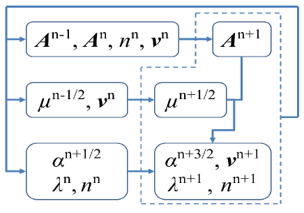
Figure 3: The complete iteration for the variational schemes of the hydrodynamic-electrodynamic model.

A very good property of the variational scheme is the conservation of Lagrangian structure generated by the discrete Lagrangian (43) $L^{n{\sim}n+1}_{d}(q^{n},q^{n+1})$, where $q^{n}=(n^{n}_{J},\bm{v}^{n}_{J},\bm{A}^{n}_{J},\phi^{n+\frac{1}{2}}_{J},\alpha^{n+\frac{1}{2}}_{J},\lambda^{n}_{J},\mu^{n-\frac{1}{2}}_{J})$ and the subscript $J$ traverses all lattice points. We define two 1-forms,

$$\bm{\theta}^{+n{\sim}n+1}=\frac{\partial}{\partial{q^{n+1}_{i}}}L^{n{\sim}n+1}_{d}\left(q^{n},q^{n+1}\right)\cdot\bm{{\rm{d}}}q^{n+1}_{i},$$ (64)

$$\bm{\theta}^{-n{\sim}n+1}=-\frac{\partial}{\partial{q^{n}_{i}}}L^{n{\sim}n+1}_{d}\left(q^{n},q^{n+1}\right)\cdot\bm{{\rm{d}}}q^{n}_{i},$$ (65)

which form a partition of the exterior derivative of the discrete Lagrangian $\bm{{\rm{d}}}L^{n{\sim}n+1}_{d}=\bm{\theta}^{+n{\sim}n+1}-\bm{\theta}^{-n{\sim}n+1}$. Then the Lagrangian noncanonical structure can be given as a closed 2-form $\bm{\Omega}^{n{\sim}n+1}_{d}=\bm{{\rm{d}}}\bm{\theta}^{+n{\sim}n+1}=\bm{{\rm{d}}}\bm{\theta}^{-n{\sim}n+1}$ as,

$$\bm{\Omega}^{n{\sim}n+1}_{d}=\frac{\partial^{2}}{\partial{q^{n}_{i}}\partial{q^{n+1}_{j}}}L^{n{\sim}n+1}_{d}\left(q^{n},q^{n+1}\right)\cdot\bm{{\rm{d}}}q^{n}_{i}\wedge\bm{{\rm{d}}}q^{n+1}_{j}.$$ (66)

This discrete geometric structure is symplectic. By using the discrete dynamical equations (44)-(54) and taking the exterior derivative of action $S_{d}$, we obtain,

$$\bm{{\rm{d}}}S_{d}=\bm{\theta}^{+N{\sim}N+1}-\bm{\theta}^{-0{\sim}1}.$$ (67)

Eq. (67) means that one more exterior derivative of this 1-form leads to,

$$\bm{\Omega}^{N{\sim}N+1}_{d}=\bm{\Omega}^{0{\sim}1}_{d}.$$ (68)

The hydrodynamic-Maxwell system generated by Eq. (10) is naturally equipped with a continuous Lagrangian symplectic structure. The conservation of discrete Lagrangian symplectic structure indicates the discrete variational principle generates a self-consistent finite-dimensional dynamical system that is a good analog of the continuous system. We should emphasize that preserving the discrete symplectic structure in the extended system (with Lagrangian multipliers) is not a necessary and sufficient condition for preserving the geometric structures in the original system. When the dynamical system is completely integrable, the Kolmogorov-Arnold-Moser (KAM) theorem states that a weak perturbation in the Hamiltonian will not break the invariant tori of the system, which is a theoretical root to ensure the good numerical properties of the structure-preserving algorithms Hairer et al. (2002). When it comes to a general dynamical system, although the KAM theorem is not always available, many numerical experiments show that the structure-preserving algorithms still exhibit good behaviors in long-term simulations Feng and Qin (2010); Hairer et al. (2002).

It can be directly examined that the gauge and translation symmetries are also preserved in the discrete dynamical equations. By introducing an arbitrary 0-form $\psi$, we can define the discrete gauge transformation,

$$\phi^{{}^{\prime}n+\frac{1}{2}}_{i,j,k}=\phi^{n+\frac{1}{2}}_{i,j,k}-\frac{\psi^{n+1}_{i,j,k}-\psi^{n}_{i,j,k}}{\Delta{t}},$$ (69)

$$A^{{}^{\prime}n}_{xi+\frac{1}{2},j,k}=A^{n}_{xi+\frac{1}{2},j,k}+\frac{\psi^{n}_{i+1,j,k}-\psi^{n}_{i,j,k}}{\Delta{x}},$$ (70)

$$A^{{}^{\prime}n}_{yi,j+\frac{1}{2},k}=A^{n}_{yi,j+\frac{1}{2},k}+\frac{\psi^{n}_{i,j+1,k}-\psi^{n}_{i,j,k}}{\Delta{y}},$$ (71)

$$A^{{}^{\prime}n}_{zi,j,k+\frac{1}{2}}=A^{n}_{zi,j,k+\frac{1}{2}}+\frac{\psi^{n}_{i,j,k+1}-\psi^{n}_{i,j,k}}{\Delta{z}}.$$ (72)

Substituting Eqs. (69)-(72) into the discrete Lagrangian density (38), and summing over it on a universal discrete space-time manifold, we can obtain the gauge-invariant discrete action. Based on the discrete Noether’s theorem, it gives the discrete charge conservation law Marsden and West (2001). Additionally, the discrete Lagrangian density (38) is space-time-coordinate-independent, which means that the discrete action is translation-invariant. Based on the discrete Noether’s theorem, the Lagrangian momentum maps preserve the general energy-momentum density Marsden and West (2001). The advantages of variational schemes in long-term simulations are ensured by the conservation of the discrete symplectic 2-form, gauge, and translation symmetries, which lead to the conserved quantities having long-term conservation and accuracy in simulations.

The variational schemes constructed here are recognized as a structure-preserving Eulerian algorithm, which is convenient to implement and parallelize. There are also other types of structure-preserving algorithms constructed for hydrodynamic-electrodynamic systems, such as the symplectic Smoothed-Particle-Hydrodynamics (SPH) method used for simulating the double-fluid model of plasmas Xiao et al. (2016). The symplectic SPH method is a Hybrid-Eulerian-Lagrangian (HEL) algorithm which avoids constraints and is suitable for simulating plasma waves. But the metaparticle interpolation is tedious and time-consuming. The Eulerian form of the variational schemes in this work without tedious interpolation is more suitable for nano-optics, although the constraints may have a singular performance under a few conditions. As the Lagrangian multipliers are pure mathematical variables, their initialization is only determined by Eqs. (45) -(47). After the physical variables are initialized self-consistently, we can obtain the initial conditions of multipliers and Lin’s constraint field by solving Eqs. (45)-(47).

III.3 Algebraic solvers

To implement the variational scheme, the solving procedure for nonlinear algebraic equations (44)-(47), (52), and (54) is a core technique. In this work, we introduce the Newton-Krylov-type methods as primary algebraic solvers Brown and Saad (1990). As the shell of a Newton-Krylov-type method, the Newton-Raphson algorithm is used as the basic nonlinear iterative method which approximates and corrects the algebraic system in every numerical step.

The nonlinear equations (44)-(47), (52), and (54) can rewritten in matrix form as,

$$\bm{F}\left(\bm{X}^{n+1}\right)=0,$$ (73)

where $\bm{F}$ is a well-defined nonlinear vector function, $\bm{X}=(\alpha_{J},v_{xJ},v_{yJ},v_{zJ},n_{J},\lambda_{J})^{T}$, and the subscript $J$ traverses all lattice points. Then the Newton-Raphson iteration is given as,

$$\bm{X}^{*}=\bm{X}-\bm{J}^{-1}_{F}\left(\bm{X}\right)\bm{F}\left(\bm{X}\right),$$ (74)

where $\bm{X}^{*}$ indicates new variables, and the Jacobian $\bm{J}_{F}$ should be updated in every iteration step. The detailed Jacobian elements can be found in App. A. The criterion $||\bm{X}^{*}-\bm{X}||/||\bm{X}||<\varepsilon$ is used to cutoff the iteration, where $\varepsilon$ is a specified sufficiently small value.

During every iteration step, we face a Jacobian inversion, which means a linear algebraic matrix equation needs to be solved. Based on the Krylov subspace theory, there are many efficient linear solvers. For example, the Generalized-Minimum-Residual (GMRES) method, the Incomplete-Cholesky-Conjugate-Gradient (ICCG) method, and the BICGSTAB method, have been constructed to solve a large sparse matrix equation Saad and Schultz (1986); Meijerink and H. A. van der Vorst (1977); H. A. van der Vorst (1992). In this work, the BICGSTAB method is introduced as the basic linear solver, because of its efficiency, stability, and parallel ability H. A. van der Vorst (1992). An alternative approach to solve the linear equations generated in nonlinear iteration is the Jacobian-Free Newton-Krylov (JFNK) method, which replaces $\bm{J}_{F}\bm{X}^{*}$ with $\bm{J}_{F}\bm{X}^{*}\approx[\bm{J}_{F}(\bm{X}+\xi\bm{X}^{*})-\bm{J}_{F}(\bm{X})]/\xi$, where $\xi$ is a small perturbation Brown and Saad (1990); Knoll and Keyes (2004). A good feature of the JFNK method is that the Jacobian-vector product can be probed approximately without forming and storing the Jacobian elements. In this work, we just use the Newton-BICGSTAB iteration method to solve the nonlinear system, as the Jacobian can be exactly derived conveniently (App. A). The JFNK approximation will be taken into consideration to accelerate the simulation in future work.

IV Numerical Experiments

IV.1 Bulk Plasmon

The first numerical experiment implemented in this work is the one-dimensional (1-D) bulk plasmon oscillation. This simulation is a numerical benchmark that is used to verify the variational code. In this 1-D simulation, the metal is specified as silver, which means the the plasma frequency $\omega_{p}=1.37\times 10^{16}$ $\mathrm{Hz}$ (for more details, see Sec.IV.2). Then the spatial step is chosen as $0.01c/\omega_{p}$, and the temporal step is determined by the Courant-Friedrichs-Lewy (CFL) constraint, where $CFL=0.5$. The numerical simulation domain is a 5000 1-D lattice, and the Message Passing Interface (MPI) is used as a parallel strategy. At the initial time, a random perturbation of gauge field is introduced as the initial condition. After 10000 steps simulation, the dispersion relation can be reconstructed by taking the Fast Fourier Transform (FFT) of the gauge field. Fig. 4 shows the evolution of the gauge field in the simulation, where the plasmon oscillation with frequency $\omega_{p}$ can be recognized obviously. Fig. 5 plots the numerical dispersion relation versus the analytical one. The numerical result (contour plot) has a good consistency with the analytical dispersion relation (solid line) in the truncation region $k\in$ [0.00057,1.4] $\times 10^{10}$m^-1. It shows that the accurate linear response has been reached over a wide range of the spectrum, which means the simulated plasmonic system is physically correct.

Figure 4: The evolution of the gauge field in the simulation of bulk plasmon oscillation.

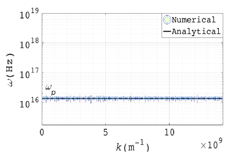
Figure 5: Bulk plasmon dispersion relations: the numerical result (contour plot) versus the analytical one (solid line).

To illustrate the good property of variational schemes in secular simulations, we plot the evolution of numerical error of total Hamiltonian, which is shown in Fig. 6 (c). After a long term simulation, the numerical error is bounded by a very small value without coherent accumulation. From the sub-Fig. 6 (a) and (b), we can find that the perturbation energy is exchanged cycle by cycle with frequency $\omega_{p}$ between the electron and field components during the oscillation, which drives the plasmonic motion.

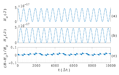
Figure 6: Numerical error of the Hamiltonian in the simulation: (a) the Hamiltonian of losslossless free electron gas; (b) the Hamiltonian of self-consistent gauge field; (c) the total Hamiltonian error. The unit of Hamiltonian is Joule.

The result of first numerical experiment provide us with a basic verification of the numerical code used for simulating plasmonic phenomena. The advantage in conservation shown by numerical error is a footstone of secular simulation for a nonlinear system.

IV.2 SPPs

A typical SPPs configuration is the infinite interface between metal and air. When it comes to silver, the average electron number density $n_{0}\approx 5.90\times 10^{28}$ $\mathrm{m}^{-3}$, and then the plasma frequency $\omega_{p}=\sqrt{n_{0}e^{2}/\epsilon_{0}m}=1.37\times 10^{16}$ $\mathrm{Hz}$. Based on the Drude model, the metallic permittivity can be given as $\epsilon(\omega)=1-\omega^{2}_{p}/\omega^{2}$. The SPPs dispersion relation can be analytically given as $k_{x}=k_{0}\sqrt{\epsilon/(\epsilon+1)}$, where $k_{0}$ is the vacuum wave number, and then the SPR frequency $\omega_{sp}=0.97\times 10^{16}$ $\mathrm{Hz}$. Fig. 7 shows the 2-D SPP configuration used in the simulations. The numerical simulation domain is a $200\times 150$ (metal $200\times 50$) uniform 2-D lattice, where the periodic boundaries are used in the x-direction, the absorbing boundaries of gauge field components are used in the z-direction, and the hard boundaries of free electron gas are used in the z-direction. The TM mode SPPs with several vacuum wave lengthes (300, 280, 260, 240, 220, 200) nm are simulated. In each simulation, the spatial step $\Delta{x}=\Delta{z}$ is $0.05\times{2\pi}/k_{x}$, the temporal step $\Delta{t}$ is determined by the CFL constraint $CFL=0.5$, and the total simulation time is 4000 steps. To effectively implement the simulations, the MPI is used to parallel the code.

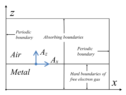
Figure 7: The 2-D SPP configuration used in the simulations.

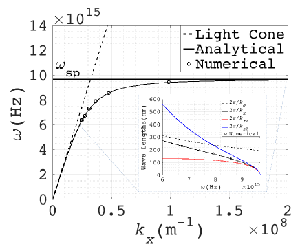
Figure 8: SPPs dispersion relations. Analytical vs numerical. Numerical results obtained at given wave lengths have a good consistency with the analytical curve. The inset plots the wave lengths and decay lengths at simulation region, which illustrates the sub-wavelength and energy localization of SPPs.

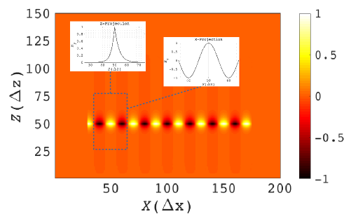
Figure 9: The slice of normalized SPPs field $H_{y}$ obtained by simulations. The vacuum wave length $\lambda_{0}=240$ nm. The insets plot the X- and Z- projections of $H_{y}$ at the region [35,65]$\times$[25,75]. It shows that the electromagnetic field of SPPs is strongly bounded by the interface, and the mode has a sub-wavelength spatial structure.

Fig. 8 shows the dispersion relation at given wave lengths obtained by simulations. By comparing the numerical results (circle marks) with analytical dispersion curve, we find that the simulations can reproduce characteristic dispersion relation of SPPs from near light cone to SPR regions. The resonance of wave means super resolution which is a core property of near field optics. The inset of Fig. 8 plots the wave lengths and decay lengths in the simulation region. It shows that the SPPs wave length (black line) and metallic decay length (red line) are always less than the vacuum wave length (dashed line), but the air decay length (blue line) is less than the vacuum wave length only in the near SPR region ($\omega>$7.9$\times 10^{15}$Hz). The numerical results of SPPs wave lengths also have a good precision. Fig. 9 shows the slice of normalized SPPs field $H_{y}$ obtained by simulations, where the vacuum wave length $\lambda_{0}=240$ nm. The Z-projection of Fig. 9 provide us with the SPPs mode structure on different sides of the silver-air interface. The localization of wave means subwavelength field structure and localized energy enhancement which can be used in many branches of nano-electrodynamics. Just as the first numerical experiment, the conserved quantities, such as the total Hamiltonian, in these simulations are still bounded by the discrete conservation laws.

The numerical experiments implemented in this work verify the numerical schemes and show the good properties of these schemes in secular simulations. It can be expected that this work will provide us with a powerful numerical tool for the first-principle based simulation study of plasmonics.

V Conclusion

In this work, we have constructed a class of variational schemes for the hydrodynamic-electrodynamic model of lossless free electron gas in quasi-neutral background to implement high-quality simulations of the SPPs. The Lagrangian density of lossless free electron gas with a self-consistent electromagnetic field was established, and the conservation laws with constraints were obtained. By using the DEC-based discretization, we reconstructed a field theory on the discrete space-time manifold and constructed the variational schemes by discretizing and minimizing the action. The variational schemes are nonlinear semi-explicit, which means the nonlinear solvers are needed. We introduced a hybrid Newton-BICGSTAB method to solve the nonlinear algebraic equations involved in the variational schemes. Instead of discretizing the partial differential equations, the variational schemes have superior numerical properties in secular simulations, as they preserve the discrete Lagrangian symplectic structure, charge, and general energy-momentum density conservations. Two types of numerical experiments, i.e., bulk plasmon oscillation and 2-D SPPs, were implemented. The numerical results can reproduce characteristic dispersion relations of both types of plasmonic phenomena. The numerical errors of conserved quantities, e.g., the total Hamiltonian, in all examples are bounded by a small value after long-term simulations, which shows the advantages of variational schemes in secular simulations. The variational schemes constructed for the hydrodynamic-electrodynamic model can be used as a powerful numerical tool in plasmonics. Improvements, such as unstructured lattices, high-quality boundaries, more efficient algebraic solvers, and loss and interband transition of real metal, will be developed in our future work.

Appendix A The Jacobian of Nonlinear Equations

To implement the Newton-Raphson iteration, we should calculate the Jacobian of nonlinear equations in every iteration step. Here we give the detailed Jacobian elements. Assuming the nonlinear function $f_{1}(\bm{X}^{n+1})$ is defined by Eq. (44), we obtain,

$$\frac{\partial{f_{1}}}{\partial{\alpha^{n+\frac{3}{2}}_{i,j,k}}}=1,$$ (75)

$$\frac{\partial{f_{1}}}{\partial{v^{n+1}_{xi+\frac{1}{2},j,k}}}=-m\Delta{t}v^{n+1}_{xi+\frac{1}{2},j,k}-e\Delta{t}A^{n+1}_{xi+\frac{1}{2},j,k}+\frac{\Delta{t}}{\Delta{x}}\left(\alpha^{n+\frac{1}{2}}_{i+1,j,k}-\alpha^{n+\frac{1}{2}}_{i,j,k}\right),$$ (76)

$$\frac{\partial{f_{1}}}{\partial{v^{n+1}_{yi,j+\frac{1}{2},k}}}=-m\Delta{t}v^{n+1}_{yi,j+\frac{1}{2},k}-e\Delta{t}A^{n+1}_{yi,j+\frac{1}{2},k}+\frac{\Delta{t}}{\Delta{y}}\left(\alpha^{n+\frac{1}{2}}_{i,j+1,k}-\alpha^{n+\frac{1}{2}}_{i,j,k}\right),$$ (77)

$$\frac{\partial{f_{1}}}{\partial{v^{n+1}_{zi,j,k+\frac{1}{2}}}}=-m\Delta{t}v^{n+1}_{zi,j,k+\frac{1}{2}}-e\Delta{t}A^{n+1}_{zi,j,k+\frac{1}{2}}+\frac{\Delta{t}}{\Delta{z}}\left(\alpha^{n+\frac{1}{2}}_{i,j,k+1}-\alpha^{n+\frac{1}{2}}_{i,j,k}\right).$$ (78)

Assuming the nonlinear function $f_{2}(\bm{X}^{n+1})$ is defined by Eq. (45), we obtain,

$$\frac{\partial{f_{2}}}{\partial{v^{n+1}_{xi+\frac{1}{2},j,k}}}=mn^{n+1}_{i+\frac{1}{2},j+\frac{1}{2},k+\frac{1}{2}},$$ (79)

$$\frac{\partial{f_{2}}}{\partial{n^{n+1}_{i+\frac{1}{2},j+\frac{1}{2},k+\frac{1}{2}}}}=mv^{n+1}_{xi+\frac{1}{2},j,k}+eA^{n+1}_{xi+\frac{1}{2},j,k}-\frac{\alpha^{n+\frac{1}{2}}_{i+1,j,k}-\alpha^{n+\frac{1}{2}}_{i,j,k}}{\Delta{x}},$$ (80)

$$\frac{\partial{f_{2}}}{\partial\lambda^{n+1}_{i+\frac{1}{2},j+\frac{1}{2},k+\frac{1}{2}}}=-\frac{\mu^{n+\frac{1}{2}}_{i+1,j,k}-\mu^{n+\frac{1}{2}}_{i,j,k}}{\Delta{x}}.$$ (81)

Assuming the nonlinear function $f_{3}(\bm{X}^{n+1})$ is defined by Eq. (46), we obtain,

$$\frac{\partial{f_{3}}}{\partial{v^{n+1}_{yi,j+\frac{1}{2},k}}}=mn^{n+1}_{i+\frac{1}{2},j+\frac{1}{2},k+\frac{1}{2}},$$ (82)

$$\frac{\partial{f_{3}}}{\partial{n^{n+1}_{i+\frac{1}{2},j+\frac{1}{2},k+\frac{1}{2}}}}=mv^{n+1}_{yi,j+\frac{1}{2},k}+eA^{n+1}_{yi,j+\frac{1}{2},k}-\frac{\alpha^{n+\frac{1}{2}}_{i,j+1,k}-\alpha^{n+\frac{1}{2}}_{i,j,k}}{\Delta{y}},$$ (83)

$$\frac{\partial{f_{3}}}{\partial\lambda^{n+1}_{i+\frac{1}{2},j+\frac{1}{2},k+\frac{1}{2}}}=-\frac{\mu^{n+\frac{1}{2}}_{i,j+1,k}-\mu^{n+\frac{1}{2}}_{i,j,k}}{\Delta{y}}.$$ (84)

Assuming the nonlinear function $f_{4}(\bm{X}^{n+1})$ is defined by Eq. (47), we obtain,

$$\frac{\partial{f_{4}}}{\partial{v^{n+1}_{zi,j,k+\frac{1}{2}}}}=mn^{n+1}_{i+\frac{1}{2},j+\frac{1}{2},k+\frac{1}{2}},$$ (85)

$$\frac{\partial{f_{4}}}{\partial{n^{n+1}_{i+\frac{1}{2},j+\frac{1}{2},k+\frac{1}{2}}}}=mv^{n+1}_{zi,j,k+\frac{1}{2}}+eA^{n+1}_{zi,j,k+\frac{1}{2}}-\frac{\alpha^{n+\frac{1}{2}}_{i,j,k+1}-\alpha^{n+\frac{1}{2}}_{i,j,k}}{\Delta{z}},$$ (86)

$$\frac{\partial{f_{4}}}{\partial\lambda^{n+1}_{i+\frac{1}{2},j+\frac{1}{2},k+\frac{1}{2}}}=-\frac{\mu^{n+\frac{1}{2}}_{i,j,k+1}-\mu^{n+\frac{1}{2}}_{i,j,k}}{\Delta{z}}.$$ (87)

Assuming the nonlinear function $f_{5}(\bm{X}^{n+1})$ is defined by Eq. (52), we obtain,

$$\frac{\partial{f_{5}}}{\partial{v^{n+1}_{xi+\frac{1}{2},j,k}}}=\frac{\Delta{t}}{\Delta{x}}n^{n+1}_{i+\frac{1}{2},j+\frac{1}{2},k+\frac{1}{2}},$$ (88)

$$\frac{\partial{f_{5}}}{\partial{v^{n+1}_{xi-\frac{1}{2},j,k}}}=-\frac{\Delta{t}}{\Delta{x}}n^{n+1}_{i-\frac{1}{2},j+\frac{1}{2},k+\frac{1}{2}},$$ (89)

$$\frac{\partial{f_{5}}}{\partial{v^{n+1}_{yi,j+\frac{1}{2},k}}}=\frac{\Delta{t}}{\Delta{y}}n^{n+1}_{i+\frac{1}{2},j+\frac{1}{2},k+\frac{1}{2}},$$ (90)

$$\frac{\partial{f_{5}}}{\partial{v^{n+1}_{yi,j-\frac{1}{2},k}}}=-\frac{\Delta{t}}{\Delta{y}}n^{n+1}_{i+\frac{1}{2},j-\frac{1}{2},k+\frac{1}{2}},$$ (91)

$$\frac{\partial{f_{5}}}{\partial{v^{n+1}_{zi,j,k+\frac{1}{2}}}}=\frac{\Delta{t}}{\Delta{z}}n^{n+1}_{i+\frac{1}{2},j+\frac{1}{2},k+\frac{1}{2}},$$ (92)

$$\frac{\partial{f_{5}}}{\partial{v^{n+1}_{zi,j,k-\frac{1}{2}}}}=-\frac{\Delta{t}}{\Delta{z}}n^{n+1}_{i+\frac{1}{2},j+\frac{1}{2},k-\frac{1}{2}},$$ (93)

$$\frac{\partial{f_{5}}}{\partial{n^{n+1}_{i+\frac{1}{2},j+\frac{1}{2},k+\frac{1}{2}}}}=1+\frac{\Delta{t}}{\Delta{x}}v^{n+1}_{xi+\frac{1}{2},j,k}+\frac{\Delta{t}}{\Delta{y}}v^{n+1}_{yi,j+\frac{1}{2},k}+\frac{\Delta{t}}{\Delta{z}}v^{n+1}_{zi,j,k+\frac{1}{2}},$$ (94)

$$\frac{\partial{f_{5}}}{\partial{n^{n+1}_{i-\frac{1}{2},j+\frac{1}{2},k+\frac{1}{2}}}}=-\frac{\Delta{t}}{\Delta{x}}v^{n+1}_{xi-\frac{1}{2},j,k},$$ (95)

$$\frac{\partial{f_{5}}}{\partial{n^{n+1}_{i+\frac{1}{2},j-\frac{1}{2},k+\frac{1}{2}}}}=-\frac{\Delta{t}}{\Delta{y}}v^{n+1}_{yi,j-\frac{1}{2},k},$$ (96)

$$\frac{\partial{f_{5}}}{\partial{n^{n+1}_{i+\frac{1}{2},j+\frac{1}{2},k-\frac{1}{2}}}}=-\frac{\Delta{t}}{\Delta{z}}v^{n+1}_{zi,j,k-\frac{1}{2}}.$$ (97)

Assuming the nonlinear function $f_{6}(\bm{X}^{n+1})$ is defined by Eq. (54), we obtain,

$$\frac{\partial{f_{6}}}{\partial{v^{n+1}_{xi+\frac{1}{2},j,k}}}=\frac{\Delta{t}}{\Delta{x}}\lambda^{n+1}_{i+\frac{1}{2},j+\frac{1}{2},k+\frac{1}{2}},$$ (98)

$$\frac{\partial{f_{6}}}{\partial{v^{n+1}_{xi-\frac{1}{2},j,k}}}=-\frac{\Delta{t}}{\Delta{x}}\lambda^{n+1}_{i-\frac{1}{2},j+\frac{1}{2},k+\frac{1}{2}},$$ (99)

$$\frac{\partial{f_{6}}}{\partial{v^{n+1}_{yi,j+\frac{1}{2},k}}}=\frac{\Delta{t}}{\Delta{y}}\lambda^{n+1}_{i+\frac{1}{2},j+\frac{1}{2},k+\frac{1}{2}},$$ (100)

$$\frac{\partial{f_{6}}}{\partial{v^{n+1}_{yi,j-\frac{1}{2},k}}}=-\frac{\Delta{t}}{\Delta{y}}\lambda^{n+1}_{i+\frac{1}{2},j-\frac{1}{2},k+\frac{1}{2}},$$ (101)

$$\frac{\partial{f_{6}}}{\partial{v^{n+1}_{zi,j,k+\frac{1}{2}}}}=\frac{\Delta{t}}{\Delta{z}}\lambda^{n+1}_{i+\frac{1}{2},j+\frac{1}{2},k+\frac{1}{2}},$$ (102)

$$\frac{\partial{f_{6}}}{\partial{v^{n+1}_{zi,j,k-\frac{1}{2}}}}=-\frac{\Delta{t}}{\Delta{z}}\lambda^{n+1}_{i+\frac{1}{2},j+\frac{1}{2},k-\frac{1}{2}},$$ (103)

$$\frac{\partial{f_{6}}}{\partial\lambda^{n+1}_{i+\frac{1}{2},j+\frac{1}{2},k+\frac{1}{2}}}=1+\frac{\Delta{t}}{\Delta{x}}v^{n+1}_{xi+\frac{1}{2},j,k}+\frac{\Delta{t}}{\Delta{y}}v^{n+1}_{yi,j+\frac{1}{2},k}+\frac{\Delta{t}}{\Delta{z}}v^{n+1}_{zi,j,k+\frac{1}{2}},$$ (104)

$$\frac{\partial{f_{6}}}{\partial\lambda^{n+1}_{i-\frac{1}{2},j+\frac{1}{2},k+\frac{1}{2}}}=-\frac{\Delta{t}}{\Delta{x}}v^{n+1}_{xi-\frac{1}{2},j,k},$$ (105)

$$\frac{\partial{f_{6}}}{\partial\lambda^{n+1}_{i+\frac{1}{2},j-\frac{1}{2},k+\frac{1}{2}}}=-\frac{\Delta{t}}{\Delta{y}}v^{n+1}_{yi,j-\frac{1}{2},k},$$ (106)

$$\frac{\partial{f_{6}}}{\partial\lambda^{n+1}_{i+\frac{1}{2},j+\frac{1}{2},k-\frac{1}{2}}}=-\frac{\Delta{t}}{\Delta{z}}v^{n+1}_{zi,j,k-\frac{1}{2}}.$$ (107)

It can be seen that the Jacobian $\bm{J}_{F}$ is a large sparse matrix in every iteration step.

References

- Ritchie (1957) R. Ritchie, Phys. Rev. 106, 874 (1957).
- Barnes et al. (2003) W. Barnes, A. Dereux, and T. Ebbesen, Nature 424, 6950:824 (2003).
- Ozbay (2006) E. Ozbay, Science 311, 5758:189 (2006).
- Zia and Brongersma (2007) R. Zia and M. L. Brongersma, nature nanotechnology 2, 426 (2007).
- Hendry et al. (2008) E. Hendry, F. Garcia-Vidal, L. Martin-Moreno, J. Rivas, M. Bonn, A. Hibbins, and M. Lockyear, Phys. Rev. Lett. 100, 123901 (2008).
- Kim et al. (2008) S. Kim, J. H. Jin, Y. J. Kim, I. Y. Park, Y. Kim, and S. W. Kim, Nature 453, 757 (2008).
- Atwater and Polman (2010) H. Atwater and A. Polman, Nature Materials 9, 205 (2010).
- Boltasseva and Atwater (2011) A. Boltasseva and H. A. Atwater, Science 331, 6015:290 (2011).
- Valev (2012) V. K. Valev, Langmuir 28, 15454 (2012).
- Fang et al. (2017) M. Fang, Z. Huang, W. E. I. Sha, and X. Wu, IEEE J. Multiscale and Multiphys. Comput. Techn. 2, 194 (2017).
- Yee (1966) K. S. Yee, IEEE Trans. Antennas Propag. 14, 302 (1966).
- Harrington (1968) R. F. Harrington, Field Computation by Moment Methods (MacMillan, New York, 1968).
- Taflove and Brodwin (1975) A. Taflove and M. E. Brodwin, IEEE Trans. Microw. Theory Tech. 23, 623 (1975).
- Taflove (1995) A. Taflove, Computational Electrodynamics: The Finite-Difference Time-Domain Method (Artech House Publisher, Boston, 1995).
- Jr. J. D. Anderson (1995) Jr. J. D. Anderson, Computational Fluid Dynamics: The Basics with Applications (McGraw-Hill, New York, 1995).
- Chen and Chen (2012) Q. Chen and B. Chen, Phys. Rev. E 86, 046704 (2012).
- Feng (1985) K. Feng, The Proceedings of 1984 Beijing Symposium on Differential Geometry and Differential Equations (Science Press, Beijing, 1985) p. 42.
- Feng and Qin (2010) K. Feng and M. Qin, Symplectic Geometric Algorithms for Hamiltonian Systems (Springer-Verlag, New York, 2010).
- Benettin and Giorgilli (1994) G. Benettin and A. Giorgilli, J. Statist. Phys. 74, 1117 (1994).
- Reich (1999) S. Reich, SIAM J. Numer. Anal. 36, 1549 (1999).
- Hairer et al. (2002) E. Hairer, C. Lubich, and G. Wanner, Geometric Numerical Integration: Structure-Preserving Algorithms for Ordinary Differential Equations (Springer, New York, 2002).
- Wu et al. (2003) Y. K. Wu, E. Forest, and D. S. Robin, Phys. Rev. E 68, 046502 (2003).
- Hairer (2005) E. Hairer, J. Sci. Comput. 25, 67 (2005).
- Chin (2009) S. A. Chin, Phys. Rev. E 80, 037701 (2009).
- Qin et al. (2016) H. Qin, J. Liu, J. Xiao, R. Zhang, Y. He, Y. Wang, Y. Sun, J. W. Burby, L. Ellison, and Y. Zhou, Nucl. Fusion 56, 014001 (2016).
- Tao (2016) M. Tao, Phys. Rev. E 94, 043303 (2016).
- Morrison (2017) P. J. Morrison, Phys. Plasmas 24, 055502 (2017).
- Chen et al. (2017) Q. Chen, H. Qin, J. Liu, J. Xiao, R. Zhang, Y. He, and Y. Wang, J. Comput. Phys. 349, 441 (2017).
- Morrison (1998) P. J. Morrison, Rev. Mod. Phys. 70, 467 (1998).
- Marsden and West (2001) J. E. Marsden and M. West, Acta Numerica 10, 357 (2001).
- Lew et al. (2004) A. Lew, J. E. Marsden, M. Ortiz, and M. West, Int. J. Numer. Meth. Engr. 60, 153 (2004).
- West (2004) M. West, Variational Integrators, Ph.D. thesis, California Institute of Technology (2004).
- Qin and Guan (2008) H. Qin and X. Guan, Phys. Rev. Lett. 100, 035006 (2008).
- Li et al. (2011) J. Li, H. Qin, Z. Pu, L. Xie, and S. Fu, Phys. Plasmas 18, 052902 (2011).
- Squire et al. (2012a) J. Squire, H. Qin, and W. M. Tang, Phys. Plasmas 19, 052501 (2012a).
- Squire et al. (2012b) J. Squire, H. Qin, and W. M. Tang, Phys. Plasmas 19, 084501 (2012b).
- Xiao et al. (2013) J. Xiao, J. Liu, H. Qin, and Z. Yu, Phys. Plasmas 20, 102517 (2013).
- Zhang et al. (2014) R. Zhang, J. Liu, Y. Tang, H. Qin, J. Xiao, and B. Zhu, Phys. Plasmas 21, 032504 (2014).
- Stamm and Shadwick (2014) A. B. Stamm and B. A. Shadwick, IEEE Trans. Plasma Sci. 42, 1747 (2014).
- Shadwick et al. (2014) B. A. Shadwick, A. B. Stamm, and E. G. Evstatiev, Phys. Plasmas 21, 055708 (2014).
- Xiao et al. (2015) J. Xiao, J. Liu, H. Qin, Z. Yu, and N. Xiang, Phys. Plasmas 22, 092305 (2015).
- Kraus et al. (2017) M. Kraus, K. Kormann, P. J. Morrison, and E. Sonnendrücker, J. Plasma Phys. 83, 905830401 (2017).
- Shi et al. (2018) Y. Shi, J. Xiao, H. Qin, and N. J. Fisch, Phys. Rev. E 97, 053206 (2018).
- Newcomb (1962) W. Newcomb, Nucl. Fusion Suppl. part2, 451 (1962).
- Sahraoui et al. (2003) F. Sahraoui, G. Belmont, and L. Rezeau, Phys. Plasmas 10, 1325 (2003).
- Hirani (2003) A. N. Hirani, Discrete Exterior Calculus, Ph.D. thesis, California Institute of Technology (2003).
- Hiptmair (2001) R. Hiptmair, Numer. Math. 90, 265 (2001).
- Arnold et al. (2006) D. N. Arnold, R. S. Falk, and R. Winther, Acta Numer. 15, 1 (2006).
- Arnold et al. (2010) D. N. Arnold, R. S. Falk, and R. Winther, Bull. New Ser., Am. Math. Soc. 47, 281 (2010).
- Holst and Stern (2012) M. Holst and A. Stern, Found. Comput. Math. 12, 263 (2012).
- Xiao et al. (2016) J. Xiao, H. Qin, P. J. Morrison, J. Liu, Z. Yu, R. Zhang, and Y. He, Phys. Plasmas 23, 112107 (2016).
- Brown and Saad (1990) P. N. Brown and Y. Saad, SIAM J. Sci. Stat. Comput. 11, 450 (1990).
- Saad and Schultz (1986) Y. Saad and M. H. Schultz, SIAM J. Sci. Stat. Comput. 7, 856 (1986).
- Meijerink and H. A. van der Vorst (1977) J. A. Meijerink and H. A. van der Vorst, Math. Comput. 31, 148 (1977).
- H. A. van der Vorst (1992) H. A. van der Vorst, SIAM J. Sci. Stat. Comput. 13, 631 (1992).
- Knoll and Keyes (2004) D. A. Knoll and D. E. Keyes, J. Comput. Phys. 193, 357 (2004).