Joint bi-modal image reconstruction of DOT and XCT with an extended Mumford-Shah functional

Abstract

Feature similarity measures are indispensable for joint image reconstruction in multi-modality medical imaging, which enable joint multi-modal image reconstruction (JmmIR) by communication of feature information from one modality to another, and vice versa. In this work, we establish an image similarity measure in terms of image edges from Tversky’s theory of feature similarity in psychology. For joint bi-modal image reconstruction (JbmIR), it is found that this image similarity measure is an extended Mumford-Shah functional with a priori edge information proposed previously from the perspective of regularization approach. This image similarity measure consists of Hausdorff measures of the common and different parts of image edges from both modalities. By construction, it posits that two images are more similar if they have more common edges and fewer unique/distinctive features, and will not force the nonexistent structures to be reconstructed when applied to JbmIR. With the $\Gamma$-approximation of the JbmIR functional, an alternating minimization method is proposed for the JbmIR of diffuse optical tomography and x-ray computed tomography. The performance of the proposed method is evaluated by three numerical phantoms. It is found that the proposed method improves the reconstructed image quality by more than $10\%$ compared to single modality image reconstruction (SmIR) in terms of the structural similarity index measure (SSIM)

Keywords: Single-modal image reconstruction (SmIR), joint multi-modal image reconstruction (JmmIR), joint bi-modal image reconstruction (JbmIR), image similarity measures, extended Mumford-Shah functional, diffuse optical tomography (DOT), x-ray computed tomography (XCT).

1 Introduction

Biomedical imaging aims at visualizing structural or functional information necessary for medical research and clinical diagnosis. Each imaging modality can provide images of one particular physical, physiological, or biological distribution. Multi-modality medical imaging technique is to combine multiple imaging modalities into one hybrid imaging system, such as PET/MRI [Judenhofer et al., 2008, Catana, 2017], PET/XCT [Cherry, 2009, Bockisch et al., 2009, Delbeke et al., 2009, Even-Sapir et al., 2009, Kaufmann and Di Carli, 2009], SPECT/XCT [Cherry, 2009, Bockisch et al., 2009, Delbeke et al., 2009, Even-Sapir et al., 2009, Kaufmann and Di Carli, 2009], XCT/MRI [Wang et al., 2015], DOT/MRI [Panagiotou et al., 2009] and DOT/XCT [Yuan et al., 2010, Boas, 2014, Deng et al., 2015, Baikejiang et al., 2017], BLT/DOT/XCT [Yang et al., 2015], and an omni-tomography system of multiple modalities [Wang et al., 2012]. Hybrid multi-modality imaging systems can visualize anatomical and functional structures simultaneously, improve the overall imaging performance, especially avoiding the tempo-spatial artifacts because of scanning with different devices at different time and positions [Townsend, 2008]. It offers significant diagnostic advantages that cannot be achieved by a single modality [Steiner, 2007]. Moreover, if hybrid multi-modality imaging systems are perfectly calibrated, image registration is not necessary. Multi-modality medical imaging within one hybrid imaging system is called hardware fusion in [Townsend, 2008].

For single-modal image reconstruction (SmIR), theories as well as algorithms have already been well developed [Natterer et al., 2002, Scherzer, 2010, Censor et al., 2008]. Image reconstructions for hybrid multi-modality imaging systems can be conducted in several ways. The first approach is that all the image reconstructions are conducted separately by multiple SmIRs without sharing information across imaging modalities, which is a simple application of multiple SmIRs for each modality. The second approach is that all the image reconstructions are conducted sequentially by using reconstructed images to guide the next image reconstruction. The sequential reconstructions are usually started from high resolution imaging modalities such as XCT or MRI. The structural information of reconstructed images is used to guide the next reconstructions by applying structural similarity. This approach is based on the observation that images of the same object possess similar structural information, especially at key structures or strong image edges, though with different contrasts from different modalities, because they are images of the same anatomical structure. This approach is called model fusion in [Haber and Gazit, 2013] or software fusion in [Townsend, 2008]. The third approach is that all the image reconstructions are jointly conducted by sharing reciprocally structural information from one modality to another, and vice versa. This is called joint inversion in [Haber and Gazit, 2013] and joint multi-modal image reconstruction (JmmIR) in this paper. For the joint bi-modal image reconstruction such as DOT/XCT in this paper, it is called joint bi-modal image reconstruction (JbmIR).

JmmIR can be achieved by using iteratively model fusion with an appropriate image similarity measure of structural information in certain feature space for images of the underlying modalities [Haber and Gazit, 2013]. Given such an image similarity measure, the image structural feature from one modality can guide the reconstruction and help to improve the image quality of another modality, and vice versa, in one joint reconstruction process, mostly in an alternatively iterative manner. Model fusion only applies the structural information from one reconstructed image unidirectionally to improve the next reconstruction, but not vice versa. Unlike model fusion, the structural information of images in a JmmIR process is not from an image already reconstructed, but is built up progressively during the joint reconstruction process and applied reciprocally among images of underlying modalities. It is expected that JmmIR can be jointly performed with enhanced image quality but less measured data via the reciprocal communication of structural feature information. Nevertheless, the success of JmmIR relies on both the representation of image structural features of different modalities and the similarity measure between the features.

Image edge is the fundamental representation of structural information of image [Marr, 1982]. In this work, we derive an image similarity measure of image edges from Tversky’s theory of feature similarity in psychology and apply it to the JbmIR for DOT and XCT. For JbmIR, it is found that the derived image similarity measure is relevant to the extended Mumford-Shah functional with a priori edge information proposed previously for model fusion from the perspective of regularization approach in [Page, 2015]. This image similarity measure consists of Hausdorff measures of the common and different parts of image edges from DOT and XCT, and can be approximated with edge indicator functions by the $\Gamma$-convergence theory. With the $\Gamma$-approximation of the JbmIR functional, an alternating minimization method is proposed for the JbmIR of DOT and XCT. The performance of the proposed method is evaluated with three numerical phantoms. It is found that the proposed method improves the image quality by more than $10\%$ in terms of the structural similarity index measure (SSIM) for both XCT and DOT.

The structure of the paper is as follows. We first review the previous work on model fusion and JmmIR in § 2. Then in § 3 we derive an image similarity measure of image edges from Tversky’s theory of feature similarity in psychology and propose a method for JbmIR based on image edge in § 4. In § 5 we propose a heuristic $\Gamma$-approximation for the proposed JbmIR method. In § 6 we apply the JbmIR method to the JbmIR of XCT and DOT with an alternating minimization algorithm for the implementation of the method. In § 7, we perform numerical experiments with three phantoms with single modal image reconstruction with the Mumford-Shah (SmIR-MS) regularization with our JbmIR algorithm (JbmIR-MS). We discuss the results, relevant issues and future work in § 8. We conclude this paper in § 9.

2 Related work

Since JmmIR can be achieved by using iteratively model fusion, we review the previous methods for model fusion and discuss the challenges for JmmIR in this section. The following classification of methods is based on the major characteristics of methods, and is used to address the challenges for JmmIR, but is not intended to be a strict classification. There are certainly overlaps among the classifications, e.g., derivatives or its discretization, finite differences, are used explicitly or implicitly in almost all the methods.

2.1 Segmentation-based model fusion

For model fusion with MRI or CT, image edges from MRI or CT are used to replace the line process in the Gibbs distribution of [Geman and Geman, 1984]. This approach is first used for the reconstruction of PET or SPECT [Leahy and Yan, 1991, Fessler et al., 1992, Gindi et al., 1993]. If the edge information from MRI is imperfect and if the edge process is improperly weighted, using such information “blindly” can even lead to artifacts [Fessler et al., 1992, Zhang et al., 1994, Bowsher et al., 1996]. In [Bowsher et al., 1996], a simultaneous segmentation and reconstruction method for emission computed tomography (ECT) image by incorporating high-resolution anatomical information such as CT or MRI is proposed and evaluated with SPECT and MRI. Higher prior probabilities are assigned to ECT segmentations in which each ECT region stays within a single anatomical region in this incorporation [Bowsher et al., 1996]. In [Sastry and Carson, 1997] , a different method for the incorporation of anatomical information into PET image reconstruction is proposed: segmentations of MRI images are used to assign tissue composition to PET image pixels, while PET images are modeled as the sum of activities of each tissue type, weighted by the assigned tissue composition.

If segmentation from a high resolution imaging modality is available, a priori structural information is used for DOT, as the weight for an anisotropic regularization to preserve the edges in the DOT image under reconstruction in [Douiri et al., 2007]. The idea of [Douiri et al., 2007] is later applied for PET in [Chan et al., 2009] and for SPECT in [Kazantsev et al., 2012, Dewaraja et al., 2010]. For the model fusion of DOT with XCT, a similarity measure with a Laplacian-type smoothing operator within each region is proposed to average the DOT image within a region, respectively, while allowing discontinuity between different regions. [Brooksby et al., 2005, Brooksby et al., 2006, Yalavarthy et al., 2007, Baikejiang et al., 2017]. In [Fang et al., 2010, Boas, 2014, Deng et al., 2015], an empirical compositional relationship between the x-ray intensities for adipose and fibroglandular tissue is further proposed with the segmentation information from XCT, and used to guide the reconstruction of DOT in [Fang et al., 2010, Boas, 2014, Deng et al., 2015].

This approach requires both accurate anatomical image segmentation and registration [Fessler et al., 1992, Gindi et al., 1993, Ouyang et al., 1994, Sastry and Carson, 1997].

2.2 Segmentation-free model fusion

To resolve the difficulty in accurate anatomical image segmentation, information theoretic regularization using the mutual information or joint entropy to measure image similarity of image intensities are studied in [Nuyts, 2007, Tang and Rahmim, 2009, Panagiotou et al., 2009, Somayajula et al., 2011]. MRI is used as the information theoretic anatomical prior for the reconstruction of PET in [Somayajula et al., 2011] and DOT in [Panagiotou et al., 2009]. It is found that the joint entropy is more robust than the mutual information to differences between the image under reconstruction and the anatomical image provided, especially when the anatomical image has structures that are not present in the image under reconstruction [Nuyts, 2007, Tang and Rahmim, 2009, Panagiotou et al., 2009, Somayajula et al., 2011].

However, because both information theoretic metrics are based on global distributions of the image intensities, mutual information or joint entropy between images is not directly affected by local spatial structure of the images. “A random spatial reordering of corresponding pairs of voxels in the two images would produce identical measures” [Somayajula et al., 2011]. Therefore, It is necessary to incorporate features that capture the local variation in image intensities. In [Somayajula et al., 2011], scale-space features, such as a Gaussian-blurred image and its Laplacian, are added into the similarity measure to help the joint entropy reconstruction. This method is related to the following derivative-based approach.

Another disadvantage of information theoretic regularization is that it is prone to different image contrast ranges from different modalities and may lead to undesired reconstruction results [Panagiotou et al., 2009, Somayajula et al., 2011, Weizman et al., 2016].

2.3 Derivative-based model joint reconstruction

As mentioned in the introduction, unlike model fusion, the structural information in a JmmIR process is not from an image already reconstructed, but is updated progressively during the joint reconstruction process. Most of the model fusion methods in § 2.1 and § 2.2 have not been adopted to JmmIR, because of challenges in progressively computing image segmentations and quantifying similarity of image structural features of different contrast ranges from different modalities.

Another image representation, the gradient of an image serves as a convenient image edge detector and is independent of image contrast ranges [Marr and Hildreth, 1980, Canny, 1986, Perona and Malik, 1990]. The gradient and higher order derivatives such as Laplacian of an image provide alternative structural representations to resolve the aforementioned issues. They are easy to be updated progressively. With derivatives as the image structural representation, the problem is how to define the similarity measure of image structures.

This approach was first applied in geophysical imaging from multiple physical process [Haber and Oldenburg, 1997]. In [Haber and Oldenburg, 1997], the $L^{2}$-norm of second order derivatives of image differences is used as the similarity measure for the joint inversion of gravity and seismic tomography data. A generalized cross-gradient procedure is developed for joint multiple parameter inversion in [Gallardo, 2007, Gallardo and Meju, 2011], where cross-products of imaging gradients are utilized to measure the parallelism of gradients, a.k.a., the structural similarity of physical parameters.

The total variation is one of the most widely used regularizations in image reconstruction problems [Rudin et al., 1992]. For JmmIR, the joint total variation by summing up the total variations of images is used to solve the joint inversion problem in [Haber and Gazit, 2013]. However, such a joint total variation encourages the joint sparsity but not the similarity of image gradients. In [Rigie and La Riviere, 2015], the total nuclear variation (TNV) is proposed for encouraging common edge locations and alignment of their gradient vectors, and is applied to the multi-spectral CT reconstruction. In [Knoll et al., 2017], the second order total generalized variation (TGV) with nuclear-norm is applied for the joint image reconstruction of MRI and PET. It is found that the TGV nuclear norm is robust regarding unwanted transfer of individual features to other channels [Knoll et al., 2017].

In [Ehrhardt et al., 2015], for the JbmIR of PET ($u_{1}$) and MRI ($u_{2}$), another image similarity measure for image gradients is proposed to measure the parallelism of image gradients as follows, called parallel level sets (PLS),

$$\text{PLS}_{\beta}(u_{1},u_{2})=\int_{\Omega}\varphi\left[\psi\left(\|\nabla u_{1}\|_{\beta}\cdot\|\nabla u_{2}\|_{\beta}\right)-\psi\left(|\langle\nabla u_{1},\nabla u_{2}\rangle|_{\beta^{2}}\right)\right]$$ (1)

where $\Omega\subset\mathbb{R}^{N}$ is a domain that contains the object to be imaged, for $N=2$ or $3$, $\|z\|_{\beta}=(\|z\|^{2}+\beta^{2})^{\frac{1}{2}}$ for some $\beta>0$ for the differentiability of $\text{PLS}_{\beta}$, $\langle\cdot,\cdot\rangle$ is the Euclidean inner product, $\phi$ and $\psi$ are strictly increasing functions. Please note that this image similarity measure is symmetric in $u_{1}$ and $u_{2}$. Please note that asymmetric PLS can be formulated along the same framework [Ehrhardt, 2015].

However, the above derivative-based methods depend on the magnitude of gradients. For JmmIR, images tend to have different ranges of contrasts and different heights and signs of edges detected with derivatives [Rasch et al., 2017]. Normalized PLS can be formulated to resolve this issue within the framework in [Ehrhardt, 2015]. Another approach to resolve this issue is using the infimal convolution of generalized Bregman distances to formulate weighted similarity measure for image gradients without the edge orientation constraint [Rasch et al., 2017], where asymmetric weightings are also possible. This approach has also the advantage for joint reconstruction to avoid the artificial transfer of non-shared structures between the images [Rasch et al., 2017].

2.4 Summary

All work reviewed above are valuable contributions because they demonstrate the performance and advantages of JbmIR over SmIR in a number of multi-modal imaging applications. All the methods in this subsection use image gradients or derivatives as the image structural representation. Similarity measures are proposed to measure the parallelism or correlation of image gradients or derivatives, respectively. In spite of their demonstrated success, none of them is working directly on image edge. For image reconstruction, feature reconstruction [Louis, 2011] provides the possibility for directly addressing structural information on features like image edges, but has not yet been used for joint multi-modal image reconstruction. It is our motivation to develop an approach directly with image edge together with an appropriate similarity measure, which is expect to be more robust to data noise than the derivative-based methods.

As discussed in [Haber and Gazit, 2013], the challenges in JmmIR are as follows. The first fundamental challenge is because of the difference of contrast ranges or different scales of different imaging modalities [Rasch et al., 2017], or different physical meaning (and units) [Haber and Gazit, 2013]. Because structural similarity is the only clue for JmmIR, the second one is an appropriate representation of image structural information, which should support to capture the local variation in image intensities, be independent of image contrasts, and be updated progressively during the joint reconstruction process. Consequently the third one is an appropriate similarity measure for the representation of image structural information. There could be features in one modality but nonexistent in another. Hence, an appropriate similarity measure should encourage the reconstruction of features only if there is sufficient evidence from measured data support but should not force the nonexistent features to be reconstructed in another.

In this work, image edge is used as the structural representation of images, which is the line-process in the Gibbs distribution of [Geman and Geman, 1984], and edge set in the Mumford-Shah functional [Mumford and Shah, 1989]. This representation meets the criteria of the second challenge aforementioned. A similarity measure for image edge sets is derived from the feature contrast model of similarity in psychology by Tversky [Tversky, 1977], which is appropriate in the sense of the third challenge aforementioned.

3 Similarity measures for image edges

Many similarity measures explain similarity (or dissimilarity) as a distance $d(\cdot,\cdot)$ in a metric space $\mathcal{X}$ of perceptual stimulus of objects, with $d$ satisfying the following metric axioms [Tversky, 1977],

1. Minimality: $d(K_{1},K_{2})\geq d(K_{1},K_{1})=0$.

2. Symmetry: $d(K_{1},K_{2})=d(K_{2},K_{1})$.

3. Triangle inequality: $d(K_{1},K_{2})+d(K_{2},K_{3})\geq d(K_{1},K_{3})$,

where $K_{1}$, $K_{2}$ and $K_{3}\in\mathcal{X}$. This is called the geometric model of similarity [Blough, 2001, Rorissa, 2007]. However, all three metric axioms are unnecessarily stringent and can be inconsistent with a number of psychological experiments [Tversky, 1977, Mumford, 1991, Rorissa, 2007, Skopal and Bustos, 2011, Biasotti et al., 2016]. It is realized that “Similarity isn’t a metric anyway” in [Mumford, 1991] after knowing the work of [Tversky, 1977].

In his prominent paper [Tversky, 1977], Tversky proposed his famous feature contrast model for the similarity of binary features. Let $\Delta=\{a,b,c,\cdots\}$ be the domain of objects under study. Assume that each object in $\Delta$ is represented by a set of binary features. Unlike the geometric model of similarity which represent stimulus as points in a metric space, an object $a$ is characterized by the set $A$ of features that the object $a$ possesses. Features are binary in the sense that a given feature of an object either is or is not in its set of features $A$. An example of the set of features is the image edge set of an image. Tversky proposed another set of axioms about similarity measures of binary features, which include the axioms of matching, independence, solvability, invariance, and proved mathematically that feature similarity measures must be of the following form [Tversky, 1977]

$$S(a,b)=p(A\cap B)-\gamma_{1}p(A\setminus B)-\gamma_{2}p(B\setminus A),$$ (2)

where $A$ and $B$ denote the sets of binary features associated with the objects $a$ and $b$, respectively, $\gamma_{1}$ and $\gamma_{2}$ are nonnegative constants. $p$ is an additive function such that $p(A\cap B)=p(A)+p(B)$ whenever $A\cap B=\emptyset$. This representation is called the feature contrast model and has been validated with multiple psychological experimental data sets [Tversky, 1977, Tversky and Gati, 1982] and applied in image processing applications [Santini and Jain, 1997, Santini and Jain, 1999, Rorissa, 2007]. Please note that the convention here is that the more similar $A$ to $B$, the bigger the similarity measure $S(A,B)$. This formula (2) implies that a reasonable feature similarity measure is a linear combination of the measures of their common and their distinct features.

Similarity measures thus obtained increase with addition of common features and/or deletion of distinctive features (i.e., features that belong to one object but not to the other) [Tversky, 1977]. They posit that two stimuli are more similar if they have more common features and fewer unique/distinctive features [Rorissa, 2007]. Hence, similarity measures will not force the nonexistent features to be reconstructed when applied to JmmIR as discussed in § 2.4. Actually, this point is postulated as the matching axiom in [Tversky, 1977]. Psychologically, this explains why subjects tend to pay more attention to common features than distinctive features in their similarity judgments [Tversky, 1977].

The similarity in (2) is asymmetric when $\gamma_{1}\neq\gamma_{2}$. It should address that asymmetric similarity measures are in general necessary for JmmIR. Because of different image contrasts among modalities, similarity measures should be asymmetric at least from a heuristic perspective. Some of the approaches in § 2 provide asymmetric similarity measures with demonstrated advantages. At this point, It is necessary to address one distinct approach for the model fusion of PET from MRI in [Bowsher et al., 2004], which has not been reviewed in § 2. It is a segmentation-free method with a smoothing Markov prior with weights determined by the MRI image intensities at nearby voxels. It can be used in an asymmetrical way by using only partial derivatives in certain directions [Bowsher et al., 2004, Schramm et al., 2018]. It is reported in [Schramm et al., 2018] that the PLS is slightly inferior compared to the asymmetrical Bowsher method.

For 2D images, a natural choice for the measure $p$ of image edge sets is the 1-dimensional Hausdorff measure $\mathcal{H}$, or the length of image edges. Therefore, we obtain,

$$S(u_{1},u_{2})=\mathcal{H}(K_{1}\cap K_{2})-\gamma_{1}\mathcal{H}(K_{1}\setminus K_{2})-\gamma_{2}\mathcal{H}(K_{2}\setminus K_{1}),$$ (3)

where $K_{1}$ and $K_{2}$ denote the image edge sets of images $u_{1}$ and $u_{2}$, respectively. This similarity measure of image edges is closely related to the Mumford-Shah regularization functional [Mumford and Shah, 1989]. Higher-dimensional Hausdorff measures can also be used in (3) for higher-dimensional images [Jiang et al., 2014].

4 JbmIR based on image edges

In this section, we apply the similarity measure for image edges of the previous section to JbmIR and establish a general approach for JbmIR based on image edges. Without loss of generality, we restrict to the bi-modal case and 2D case in this paper to avoid notational complexity, although the mathematical formulation can be extended to general multi-modal case.

For multi-modality imaging systems, the image reconstruction problem is to estimate images $u_{i}$ from measurement data $g_{i}$, for $i=1,2$,

$$A_{i}(u_{i})=g_{i},$$ (4)

where $A_{i}$ is the forward operator of underlying imaging modality. The Mumford-Shah functional was first proposed as a variational approach for image denoising and segmentation from the Markov random field theory [Geman and Geman, 1984]. It provides an approach for incorporating edges for the regularization of image reconstruction problems. Recently the Mumford-Shah functional has been successfully applied as a regularization method for image reconstruction problems (4)[Rondi and Santosa, 2001, Ramlau and Ring, 2007, Rondi, 2008, Klann et al., 2011, Jiang et al., 2014]. The SmIR for (4) with the Mumford-Shah regularization is as follows,

$$\text{MS}(u_{i},K_{i})=\int_{\Theta_{i}}|A_{i}(u_{i})-g_{i}|^{2}+\alpha_{i}\int_{\Omega\setminus K}|\nabla u_{i}|^{2}+\beta_{i}\mathcal{H}(K_{i}),$$ (5)

where $\Theta_{i}$ is the domain of the measurement, $K_{i}$ is the edge set of the image $u_{i}$, $\alpha_{i}$ and $\beta_{i}$ are positive regularization parameters, for $i=1,2$.

The JbmIR based on image edges is to use the similarity measure in (3) to formulate the following joint reconstruction functional

$$E(u_{1},u_{2},K_{1},K_{2})=\text{MS}(u_{1},K_{1})+\text{MS}(u_{2},K_{2})-\tau S(u_{1},u_{2}),$$ (6)

where $\tau>0$ is a regularization parameter. Please note that the minus sign “$-$” is to ensure the similarity of edge sets of images $u_{1}$ and $u_{2}$ during the joint reconstruction process because of the convention that the more similar edges, the bigger their similarity. Let

$$\Phi_{i}(u_{i},K_{i})= \int_{\Theta_{i}}|A_{i}(u_{i})-g_{i}|^{2}+\alpha_{i}\int_{\Omega\setminus K_{i}}|\nabla u_{i}|^{2}.$$ (7)

Then we find,

$$E(u_{1},u_{2},K_{1},K_{2})\\ =\Phi_{1}(u_{1},K_{1})+\Phi_{2}(u_{2},K_{2})+\beta_{1}\mathcal{H}(K_{1})+\beta_{2}\mathcal{H}(K_{2})\\ -\tau\mathcal{H}(K_{1}\cap K_{2})+\tau\gamma_{1}\mathcal{H}(K_{1}\setminus K_{2})+\tau\gamma_{2}\mathcal{H}(K_{2}\setminus K_{1}).$$ (8)

In the above equation, the terms involving only the edges $K_{1}$ and $K_{2}$ sum up to

$$\beta_{1}\mathcal{H}(K_{1})+\beta_{2}\mathcal{H}(K_{2})-\tau\mathcal{H}(K_{1}\cap K_{2})+\tau\gamma_{1}\mathcal{H}(K_{1}\setminus K_{2})+\tau\gamma_{2}\mathcal{H}(K_{2}\setminus K_{1})$$ (9)

$$= \beta_{1}\mathcal{H}(K_{1}\cap K_{2})+\beta_{1}\mathcal{H}(K_{1}\setminus K_{2})+\beta_{2}\mathcal{H}(K_{2}\cap K_{1})+\beta_{2}\mathcal{H}(K_{2}\setminus K_{1})$$ (10)

$$-\tau\mathcal{H}(K_{1}\cap K_{2})+\tau\gamma_{1}\mathcal{H}(K_{1}\setminus K_{2})+\tau\gamma_{2}\mathcal{H}(K_{2}\setminus K_{1})$$ (11)

$$= (\beta_{1}+\beta_{2}-\tau)\mathcal{H}(K_{1}\cap K_{2})+(\beta_{1}+\tau\gamma_{1})\mathcal{H}(K_{1}\setminus K_{2})+(\beta_{2}+\tau\gamma_{2})\mathcal{H}(K_{2}\setminus K_{1}).$$ (12)

By re-parametrization with the reuse of the same notations for the regularization parameters $\beta_{1}$, $\beta_{2}$, $\gamma_{1}$, and $\gamma_{2}$ to avoid notational complexity, this sum can be written as the following,

$$\Psi(K_{1},K_{2})\\ =\beta_{1}\left[\mathcal{H}(K_{1}\cap K_{2})+\gamma_{1}\mathcal{H}(K_{1}\setminus K_{2})\right]+\beta_{2}\left[\mathcal{H}(K_{1}\cap K_{2})+\gamma_{2}\mathcal{H}(K_{2}\setminus K_{1})\right].$$ (16)

In summary, the joint reconstruction functional can be written as

$$E(u_{1},u_{2},K_{1},K_{2})\\ =\sum_{i=1,j\neq i}^{2}\int_{\Theta_{i}}|A_{i}(u_{i})-g_{i}|^{2}+\alpha_{i}\int_{\Omega\setminus K_{i}}|\nabla u_{i}|^{2}+\beta_{i}\left[\mathcal{H}(K_{i}\cap K_{j})+\gamma_{i}\mathcal{H}(K_{i}\setminus K_{j})\right],$$ (17)

where $\alpha_{i}$, $\beta_{i}$ and $\gamma_{i}$ ($i=1,2$) are positive regularization parameters.

5 Variational approximation for JbmIR

In [Page, 2015], an extended Mumford-Shah functional with a priori edge information was established for image reconstruction from the perspective of regularization theory. For an image reconstruction problem $A(u)=g$ with similar notations as in (4) and (5) , if partial information of image edge can be obtained, then the following reconstruction functional is proposed in [Page, 2015],

$$\text{MS}_{K^{0}}(u,K)\\ =\int_{\Theta}|A(u)-g|^{2}+\alpha\int_{\Omega\setminus K}|\nabla u|^{2}+\beta\left[\mathcal{H}(K\setminus K^{0})+\gamma\mathcal{H}(K\cap K^{0})\right],$$ (18)

where $K_{0}$ is the partial information of image edge. Theoretical results and numerical experiments were reported in [Page, 2015]. The advantages of the extended Mumford-Shah functional were demonstrated by numerical experiments with the model fusion of DOT from XCT.

By ignoring the accurate values of parameters, we have the joint reconstruction functional in (17)

$$E(u_{1},u_{2},K_{1},K_{2})=\text{MS}_{K_{2}}(u_{1},K_{1})+\text{MS}_{K_{1}}(u_{2},K_{2}).$$ (19)

However, because none of $K_{1}$ and $K_{2}$ is fixed, it is difficult to extend the theoretical results in [Page, 2015] on existence, regularization property, $\Gamma$-approximation to the joint reconstruction functional. JbmIR based on image edge as formulated in (17) is to find the minimizer pair $\left(u_{1},u_{2},K_{1},K_{2}\right)$ given the measurement $g_{1}$ and $g_{2}$ and appropriate choice of the regularization parameters. As its native form for SmIR as in (5), the joint reconstruction functional is not easy to minimize numerically because of the difficulty of tractable edge representation in implementation. $\Gamma$-approximation is an approach to find a variational approximation for minimizing the the joint reconstruction functional. We are to propose an approximation for the joint reconstruction functional and demonstrate its performance with numerical experiments in this work, based on previous work in [Page, 2015].

In [Page, 2015], the following $\Gamma$-approximation to $\text{MS}_{K^{0}}(u,K)$ in (18) is proposed,

$$\text{MS}_{K^{0}}(u,v)\\ =\int_{\Theta_{i}}|A(u)-g|^{2}+\alpha\int_{\Omega}v^{2}|\nabla u|^{2}+\beta\left[\int_{\Omega}\left(\varepsilon|\nabla v|^{2}+\frac{(1-v)^{2}}{4\varepsilon}\right)(1+\gamma(v_{0}-v)^{2})\right],$$ (20)

where $0\leq v\leq 1$ and $0\leq v_{0}\leq 1$ are the edge indicator functions for the edge sets $K$ and $K_{0}$, respectively, i.e., $v(x)=1$ if $x\notin K$ and $v(x)=0$ if $x\in K$, with the same definition for $v_{0}$ and $K_{0}$. $\varepsilon$ controls the “width” of edges. The $\Gamma$-convergence of $\text{MS}_{K^{0}}(u,v)$ is only proved for $\gamma=0$ in [Page, 2015]. Although the $\Gamma$-approximation in (20) is proposed from an heuristic perspective, its performance is demonstrated with numerical experiments in [Page, 2015]. Based on the relation in (19), we propose the following $\Gamma$-approximation to the joint reconstruction functional $E$ in (17) as follows,

$$F(u_{1},v_{1},u_{2},v_{2})\\ =\sum_{i=1,j\neq i}^{2}\int_{\Theta_{i}}|A_{i}(u_{i})-g_{i}|^{2}+\alpha_{i}\int_{\Omega}v^{2}_{i}|\nabla u_{i}|^{2}+\beta_{i}\left[\int_{\Omega}\left(\varepsilon_{i}|\nabla v_{i}|^{2}+\frac{(1-v_{i})^{2}}{4\varepsilon_{i}}\right)(1+\gamma_{i}(v_{j}-v_{i})^{2})\right],$$ (21)

where $0\leq v_{1}\leq 1$ and $0\leq v_{2}\leq 1$ are the edge indicator functions for the edge sets $K_{1}$ and $K_{2}$, respectively. $\varepsilon_{i}$ controls the “width” of edges. As $\varepsilon_{1}\to 0+$ and $\varepsilon_{2}\to 0+$, the proposed $\Gamma$-approximation (21) is expected to $\Gamma$-converge to the functional in (16), and the edge indicator functions $v_{1}$ and $v_{2}$ are expected to converge to the characteristic functions of the edge sets $K_{1}$ and $K_{2}$, respectively, in the sense of $L^{2}$. The current formulation of the $\Gamma$-approximation (21) is based on the heuristics in [Page, 2015, § 4.5]. We are unable to prove the expected convergence mathematically, although a proof for $\gamma_{1}=\gamma_{2}=0$ might be possible by using the same method in [Page, 2015] where a lengthy proof for single modal image reconstruction with the extended Mumford-Shah function with a priori edge information is provided for $\gamma=0$. In this work we concentrate in studying numerically how the proposed method can help to improve the quality of reconstructed images.

6 JbmIR of XCT and DOT

In this section we give a brief introduction of XCT and DOT, and apply the JbmIR reconstruction method in the previous section to the JbmIR of XCT and DOT.

6.1 X-ray computed tomography

In conventional X-ray tomography, the image contrast is due to the x-ray absorption when X-ray beams pass through an object. The interaction of X-ray and the object could be a complex process. Nevertheless, the beam path in straight lines provides a good approximation for X-ray tomography in many cases. The absorption process is described by Beer’s law. Please refer to [Natterer, 2001, Louis, 1989] for more details.

Let $I(x)$ be the intensity of an X-ray and $f(x)$ the X-ray attenuation coefficient at position $x$. Then along a straight line $L$,

$$\frac{dI}{dl}=-fdl,$$ (22)

where $dl$ is the differential element along $L$. Let $I_{0}$ be the initial intensity of the X-ray and $I_{1}$ the intensity after passing through the object. As we assume that the beam travels in the straight line $L$, from (22) it follows

$$\ln\frac{I_{1}}{I_{0}}=-\int_{L}fdl.$$ (23)

The measurement $I_{1}$ and the initial intensity $I_{0}$ provide line integrals of the X-ray attenuation coefficient $f$ along lines, if the measurement is conducted in multiple directions and positions. The operator that maps a function into the set of its line integrals is the Radon Transform, which is defined as the following in the case of 2D XCT,

$$R(f)(\theta,s)=\int_{L}fdl,$$ (24)

for every line $L$ crossing the domain $\Omega\subset\mathbb{R}^{2}$ containing underlying objects, where $\theta=(\cos\varphi,\sin\varphi)$ is the normal direction of the line $L=\{(x,y)\in\mathbb{R}^{2}:\,x\cos\varphi+y\sin\varphi=s\}$ and $s\in\mathbb{R}$. Let $\Theta_{1}=S^{1}\times\mathbb{R}$ (where $S^{1}$ is the unit circle), and $u_{1}=f$, and $g_{1}=\ln\frac{I_{1}}{I_{0}}$. Then the XCT is to estimate the image $u_{1}$ from its measurement data $g_{1}$,

$$R(u_{1})=g_{1}.$$ (25)

6.2 Diffuse optical tomography

The steady-state diffuse optical tomography (DOT) is a functional imaging modality which uses near infrared light to illuminate biological tissue and reconstruct the inside distribution of optical properties using the light intensity measured on the surface of the tissue. Light at near-infrared wavelength will be absorbed and scattered while passing through biological tissue. The optical properties have direct biological relevance since the absorption of light is due to the existence of oxy-/deoxy-haemoglobin. Please refer to [Arridge, 1999, Arridge and Schotland, 2009] for more details.

The governing equation used for diffuse light $u$ in DOT is the diffuse approximation of the radiative transport equation (RTE),

$$-\hbox{div}(D\nabla u)+\mu_{a}u=0,\qquad\text{in $\Omega$}$$ (26)

where $D$ is the diffusion coefficient and $\mu_{a}$ is the absorption coefficient. The incoming light $q$ can be modeled by Robin boundary condition in the diffuse approximation,

$$u+2D\overrightarrow{n}\cdot\nabla u=q,\qquad\text{on $\partial\Omega$}$$ (27)

where $\overrightarrow{n}$ is the outer normal on the boundary $\partial\Omega$ of $\Omega$. The measurement $g_{2}$ is the negative Neumann boundary values of the solution of equation (26)

$$g_{2}=-D\overrightarrow{n}\cdot\nabla u,\qquad\text{on $\partial\Omega$}.$$ (28)

In practice, extra coupling coefficients due to refraction should be introduced into the equations (27) and (28) [Arridge, 1999, Arridge and Schotland, 2009]. Given the incoming light $q$, diffusion coefficient $D$ and absorption coefficient $\mu_{a}$, the forward operator $\mathcal{F}$ in DOT maps $(\mu_{a},D)$ to the measurement data $g_{2}$ in (28). The DOT is to estimate $(\mu_{a},D)$ from the measurement data $g_{2}$,

$$\mathcal{F}(\mu_{a},D)=g_{2}.$$ (29)

In this work we consider a special case of DOT to demonstrate the performance of the proposed JbmIR method. We are interested in recovering the absorption coefficient $\mu_{a}$, and assume the diffusion coefficient $D$ to be known in the following. This is an interesting but non-linear and ill-posed inverse problem [Arridge and Schotland, 2009]. For a known diffusion coefficient $D$, we introduce the new forward operator $G$ as

$$G(\mu_{a})=\mathcal{F}(\mu_{a},D)$$ (30)

To use the same notations in the previous sections, we write $u_{2}$ to represent the absorption image $\mu_{a}$, and $g_{2}$ for the measurement $G(\mu_{a})$. Then the DOT with know diffuse coefficient is to estimate $u_{2}$ from the measurement data $g_{2}$ ,

$$G(u_{2})=g_{2},$$ (31)

where the measurement is on the boundary $\Theta_{2}=\partial\Omega$ of $\Omega$.

6.3 JbmIR of XCT and DOT

With the development of hybrid multi-modal imaging techniques, there are a number of hybrid optical tomography systems reported in the literature together with reconstruction methods by model fusion from XCT or JbmIR with XCT, such as DOT/XCT [Yuan et al., 2010, Boas, 2014, Deng et al., 2015, Baikejiang et al., 2017], BLT/DOT/XCT [Yang et al., 2015]. To reduce the radiation dose and accelerate the data acquisition, it is the x-ray tomosynthesis technique of limited views that is used in the latter work [Baikejiang et al., 2017, Boas, 2014, Deng et al., 2015] rather than the conventional full-scan XCT.

By applying the general JbmIR formulation in (21), we obtain the following joint reconstruction function for XCT and DOT,

$$F(u_{1},v_{1},u_{2},v_{2})\\ =\int_{\Theta_{1}}|R(u_{1})-g_{1}|^{2}+\alpha_{i}\int_{\Omega}v^{2}_{1}|\nabla u_{1}|^{2}+\beta_{1}\left[\int_{\Omega}\left(\varepsilon_{1}|\nabla v_{1}|^{2}+\frac{(1-v_{1})^{2}}{4\varepsilon_{1}}\right)(1+\gamma_{1}(v_{2}-v_{1})^{2})\right]\\ +\int_{\Theta_{2}}|G(u_{2})-g_{2}|^{2}+\alpha_{2}\int_{\Omega}v^{2}_{2}|\nabla u_{2}|^{2}+\beta_{2}\left[\int_{\Omega}\left(\varepsilon_{2}|\nabla v_{2}|^{2}+\frac{(1-v_{2})^{2}}{4\varepsilon_{2}}\right)(1+\gamma_{2}(v_{1}-v_{2})^{2})\right],$$ (32)

where $0\leq v_{1}\leq 1$ and $0\leq v_{2}\leq 1$ are the edge indicator functions for the edge sets of XCT image $u_{1}$ and DOT image $u_{2}$, respectively. Please note that there are no weighting parameters in front of the two fidelity terms, but this does not mean both fidelity terms contribute equally to the joint reconstruction. Because of the alternating minimization algorithm discussed in the following, they never meet each other and their contributions are independent of each other. The difference of their contribution are weighted by the regularization parameters $\beta_{1}$, $\beta_{2}$, $\gamma_{1}$ and $\gamma_{2}$. During the training of the regularization parameters, the two fidelity terms also play roles independent of each other. The difference of their contribution, even if there are different weights for both, will merged into the regularization parameters.

The JbmIR of XCT and DOT in this work is to reconstruct the images $u_{1}$ and $u_{2}$ as well as the edge indicators $v_{1}$ and $v_{2}$ simultaneously in an iterative process. This is achieved by minimizing the objective functional (32) with an alternating minimization algorithm in the order of $u_{1}$, $v_{1}$, $u_{2}$ and $v_{2}$. Each minimization for $u_{1}$, $v_{1}$, $u_{2}$ and $v_{2}$ is a gradient descending with the backtracking line search method by the Armijo-Goldstein stopping condition [Armijo, 1966, Wikipedia contributors, 2017], with the previous reconstruction as initial value and the others being frozen at the latest reconstructed values. Hence, the proposed alternating minimization algorithm for the JbmIR of XCT and DOT is an instance of stochastic gradient descending with the aforementioned order, and is described in Algorithm 1. Notice that we use $\arg\min$ in the algorithm description to indicate our minimizing purpose and in each step we use gradient descent method, therefore the results we get from the iteration are the approximations of minimizers.

Algorithm 1 Alternating minimization for JbmIR of XCT and DOT

for $i=0,1,2,\ldots,n$ do

$$u_{1}^{i+1}= \arg\min_{u_{1}}F(u_{1},v_{1}^{i},u_{2}^{i},v_{2}^{i})$$ (33)

$$\hbox{with $u_{1}^{i}$ as the initial value};$$

$$v_{1}^{i+1}= \arg\min_{v_{1}}F(u_{1}^{i+1},v_{1},u_{2}^{i},v_{2}^{i})$$ (34)

$$\hbox{with $v_{1}^{i}$ as the initial value};$$

$$u_{2}^{i+1}= \arg\min_{u_{2}}F(u_{1}^{i+1},v_{1}^{i+1},u_{2},v_{2}^{i})$$ (35)

$$\hbox{with $u_{2}^{i}$ as the initial value};$$

$$v_{2}^{i+1}= \arg\min_{v_{2}}F(u_{1}^{i+1},v_{1}^{i+1},u_{2}^{i+1},v_{2})$$ (36)

$$\hbox{with $v_{2}^{i}$ as the initial value};$$

end for

Although there are many terms in the joint reconstruction functional $F$ in (32), there is not so many computing terms at each minimization step in (33), (34) (35) and (36) because some terms can be treated as constants. For example, at the minimization step (33), only the first two terms at the first line on the right-hand side of (32) are involved in this minimization step, those terms not involving $u_{1}$ can be treated as constants and ignored. Especially the time consuming computation of the forward process $G$ for the DOT is not needed. We have carefully analyzed the dependent terms at each minimization step to reduce the computing load. Implementation and experimental details are reported in the next section.

7 Numerical experiments

In discrete case, the gradients are discretized with forward difference and the divergence with backward difference, so that the discretized gradient corresponds to the gradient of the discretized functional.

For XCT, the initial image value is set as zero and the initial edge value is set as one. For DOT, zero and one initials cannot lead to good reconstruction results. We use gradient descent method for only the fidelity term to get a blurry image as the initial image value, and use the Mumford-Shah functional segmenting this initial image to get the initial edge value. The SmIR-MS and JbmIR-MS both use this same initial value setting.

We also need to set up the stopping criterion of our algorithm. This is achieved by setting up the iteration numbers involved. After a number of numerical experiments with phantoms of similar structures as in this work, we find that after 80 whole iterations with 10 steps for each variables in every iteration the SSIM values, which we use to evaluate the quality of the reconstructed images, of both XCT and DOT stabilize at relatively higher values, and in our examples over 0.85 for XCT and over 0.69 for DOT.

We evaluate the quality of the reconstructed image $u_{rec}$ via the structural similarity index measure (SSIM)[Wang et al., 2004] using the corresponding true image $u_{true}$ as a reference image:

$$\hbox{SSIM}(u_{rec},u_{true})=\frac{(2\overline{u}_{true}\overline{u}_{rec}+C_{1})(2\sigma_{u_{true}u_{rec}}+C_{2})}{(\overline{u}_{true}^{2}+\overline{u}_{rec}^{2}+C_{1})(\sigma_{u_{true}}^{2}+\sigma_{u_{rec}}^{2}+C_{2})}$$ (37)

where $\overline{u}_{true}$, $\overline{u}_{rec}$ are averages, $\sigma^{2}_{u_{true}}$, $\sigma^{2}_{u_{rec}}$ are variances and $\sigma_{u_{true}u_{rec}}$ is the covariance.

SSIM value is proposed to measure the similarity between two images considering three comparison measurements: luminance, contrast and structure. We use the default parameter settings that $C_{1}=(0.01L)^{2}$, $C_{2}=(0.03L)^{2}$, where $L$ is the dynamic range of the ground truth. The higher SSIM value is the more similar the two images are. SSIM=1 only happens for identical images.

7.1 Experimental setting

The computations are done using Matlab. For XCT, the Radon Transformation and the adjoint operator written by Lut Justen from the Software-Documentation of the Center for Industrial Mathematics, University of Bremen are implemented. For DOT, the TOAST++ package[Schweiger and Arridge, 2014] from Martin Schweiger and Simon Arridge is implemented for the forward operator and the Jacobian matrix of the forward operator.

For XCT, the projection data are obtained from 30 views uniformly distributed in $[0,180^{o}]$. Because our phantoms are of radius 25 mm and image sizes are of $100\times 100$ pixels, the package we use for XCT automatically assigns each view 100 uniformly distributed parallel X-ray beams with a step-length of 0.5 mm. For DOT, the data are obtained with 16 source positions and 16 detector positions. TOAST++ uses finite element method to solve DOT problem. The mesh and the positions of source and detector are shown in Figure 1.

We add additional Gaussian noise $n$ to our noise free data $d$. Since the fidelity term $\int_{\Theta_{i}}|A_{i}(u_{i})-g_{i}|^{2}$ shows that $A_{i}(u_{i})$ should be a good approximation of the data $g_{i}$ in $L_{2}$ norm, we scale the noise $n$ to the data with regard to the $L_{2}$ norm. The relative noise level is defined as $\eta=\frac{\|n\|}{\|d\|}$, where $\|\cdot\|$ is the Euclidean norm. In our numerical experiments 5% relative Gaussian noise is added to the XCT data and 2% relative Gaussian noise is added to the DOT data.

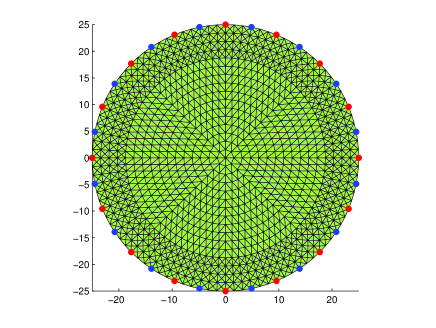
Figure 1: Finite element mesh for DOT problem with 16 source positions (red points) and 16 detector positions (blue points).

7.2 Parameter choosing

The choice of the regularization parameters is non-trivial and should be done task-dependently [Schramm et al., 2018].

In our proposed JbmIR-MS method, the “width” control parameters $\varepsilon_{1}$ and $\varepsilon_{2}$ are set as $1\times 10^{-4}$, which are the same as in [Page, 2015]. There are three regularization parameters $\alpha_{i}$, $\beta_{i}$ and $\gamma_{i}$ $(i=1,2)$ needed to be chosen properly for each modality. $\alpha_{i}$ is the regularization parameter of the smoothing penalty term. The larger it is, the smoother the reconstructed image will be when there is not any edge. $\beta_{i}$ weights how strongly the edge penalizes. The larger it is, the fewer edges will be reconstructed. $\gamma_{i}$ controls the effect of the reference edge information. The effect of the reference edge information increases as the value of $\gamma_{i}$ increases.

For JbmIR-MS, from the XCT with a priori edge information numerical experiments done by Thomas we can get that when the order of magnitude of $\alpha_{1}$ is around $10^{4}$, the order of magnitude of $\beta_{1}$ is around $10^{-3}$ or $10^{-4}$ and $\gamma_{1}$ is no more than $10$ we could be able to get XCT results with clear structures. We first fix the XCT parameters as $\alpha_{1}=9\times 10^{3},\leavevmode\nobreak\ \beta_{1}=2\times 10^{-3},\leavevmode\nobreak\ \gamma_{1}=10$ to choose DOT parameters. For joint DOT reconstruction we first roughly partition the parameter space and compute the SSIM value to find rough-optimal parameters. Then according to the reconstruction results and the parameter effect discussed above, we fine-tune the parameters around this rough-optimal choice. For example, if the reconstructed image is too smooth in non-edge area, we will decrease the value of $\alpha_{2}$. If there are too few edges, we will slightly decrease the value of $\beta_{2}$. If the influence of the reference edge information is too strong that we reconstruct wrong structures that should only appear in one modality and not in the other, we will slightly decrease the value of $\gamma_{2}$. Here $\alpha_{2}$ is chosen from $A_{2}=[0.01,0.1,\ldots,1\times 10^{9}]$, $\beta_{2}$ is chosen from $B_{2}=[1\times 10^{-9},1\times 10^{-8},\ldots,0.1,1]$, and $\gamma_{2}$ is chosen from $C_{2}=[1,2,\ldots,9,10]$. Theses parameter ranges are chosen from our experience with a number of phantoms of similar structures. For our numerical experiments, we find that $\alpha_{2}=1\times 10^{5}$, $\beta_{2}=1\times 10^{-5}$ and $\gamma_{2}=5$ produce a higher SSIM value of the reconstructed DOT image against its true image, among all possible combinations from $A\times B\times C$. Then we fine-tune this rough-optimal choice according to the discussion above and reach the parameter settings we use in our numerical experiments. After choosing the DOT parameters, we then fine-tune the joint XCT parameters around $\alpha_{1}=9\times 10^{3},\leavevmode\nobreak\ \beta_{1}=2\times 10^{-3},\leavevmode\nobreak\ \gamma_{1}=10$. The final parameter settings for every experiment are listed in the description of the numerical results.

We compare our method with SmIR using Mumford-Shah functional(SmIR-MS).

For SmIR-MS, the “width” control parameter $\varepsilon$ is also set as $1\times 10^{-4}$. There are two regularization parameters $\alpha$ and $\beta$ for each modality. The reconstruction result is sensitive to both of them. The larger $\alpha$ is the smoother the reconstructed image will be when there is not any edge. The larger $\beta$ is the fewer edges will be reconstructed. We first perform a search of the parameter space in a rough scale with the SSIM as the criterion. For both single modality reconstructions $\alpha$ and $\beta$ are chosen from $A=[0.01,0.1,\ldots,1\times 10^{9}]$ and $B=[1\times 10^{-9},1\times 10^{-8},\ldots,0.1,1]$ to determine the proper order of magnitudes first. For DOT reconstruction we find that $\alpha=1\times 10^{5}$ and $\beta=1\times 10^{-7}$ produce a higher SSIM value of the reconstructed DOT image against its true image, among all possible combinations from $A\times B$. For XCT reconstruction the parameters are $\alpha=1\times 10^{4}$ and $\beta=1\times 10^{-2}$. We then fine-tune this rough-optimal choice according to the discussion above and our final parameter settings for every experiment are listed in the description of the numerical results.

7.3 Phantom setting

We design three pairs of phantoms of size $100\times 100$. They are all circles with a radius of $25\leavevmode\nobreak\ \text{mm}$. Inside the circles, the structures are shown in Figure 2, Figure 3 and Figure 4. The X-ray attenuation coefficients $u_{1}$ and the absorption coefficients $u_{2}$ are listed in Table 1, Table 2 and Table 3.

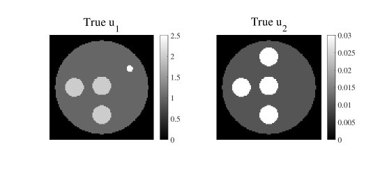
Figure 2: Phantom 1. Left: the true distribution of the X-ray attenuation coefficient $u_{1}$. Right: the true distribution of the absorption coefficient $u_{2}$.

Table 1: Phantom 1

	Background	Three circles	Top circle	small circle
XCT $u_{1}$ ($mm^{-1}$)	1	2	—	2.5
DOT $u_{2}$ ($mm^{-1}$)	0.01	0.03	0.03	—

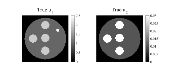
Figure 3: Phantom 2. Left: the true distribution of the X-ray attenuation coefficient $u_{1}$. Right: the true distribution of the absorption coefficient $u_{2}$.

Table 2: Phantom 2

	Background	Four circles	small circle
XCT $u_{1}$ ($mm^{-1}$)	1	2	2.5
DOT $u_{2}$ ($mm^{-1}$)	0.01	0.03	—

Figure 4: Phantom 3. Left: the true distribution of the X-ray attenuation coefficient $u_{1}$. Right: the true distribution of the absorption coefficient $u_{2}$.

Table 3: Phantom 3

	Background	Two circle and one ellipse	Top circle	small circle
XCT $u_{1}$ ($mm^{-1}$)	1	2	—	2.5
DOT $u_{2}$ ($mm^{-1}$)	0.01	0.03	0.03	—

7.4 Comparison with the SmIR

To compare the results, we put the reconstructed images of JbmIR-MS and SmIR-MS together with the true distribution, and we adjust the display window all the same as the ground truth, that is $[0,2.5]$ for XCT images and $[0,0.03]$ for DOT images. Since Mumford-Shah functional provides edge information, we also compare the reconstructed edge information using JbmIR-MS and SmIR-MS.

7.4.1 Example 1

For JbmIR-MS we choose $\alpha_{1}=8.8\times 10^{3},\leavevmode\nobreak\ \beta_{1}=1.9\times 10^{-3},\leavevmode\nobreak\ \gamma_{1}=9.8,\leavevmode\nobreak\ \alpha_{2}=1\times 10^{5},\leavevmode\nobreak\ \beta_{2}=6\times 10^{-5},\leavevmode\nobreak\ \gamma_{2}=5$. For SmIR-MS XCT, we choose $\alpha=8.8\times 10^{3},\leavevmode\nobreak\ \beta=8\times 10^{-3}.$ For SmIR-MS DOT, we choose $\alpha=1\times 10^{5},\leavevmode\nobreak\ \beta=5\times 10^{-7}.$ Figure 5 shows the reconstruction results. The three images in the first row from left to right are the true distribution of the X-ray attenuation coefficient $u_{1}$, JbmIR-MS $u_{1}$ and SmIR-MS $u_{1}$. The second row are the true distribution of the absorption coefficient $u_{2}$, JbmIR-MS $u_{2}$, and SmIR-MS $u_{2}$. According to the SSIM values, the image quality of reconstructed $u_{1}$ is improved using JbmIR-MS (SSIM from 0.79 to 0.87). The image quality of reconstructed $u_{2}$ is improved using JbmIR-MS (SSIM$=0.69$) then SmIR-MS (SSIM$=0.61$). We notice in the JbmIR-MS results that both modalities maintain their own distinct structure (small circle in XCT and top circle in DOT) and no false structure has been reconstructed because of the information communication with the other modality.

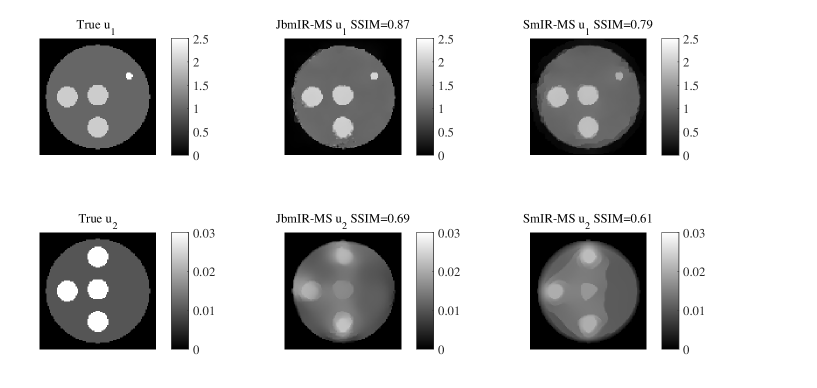
Figure 5: Phantom 1 reconstruction results. (top) The XCT phantom and reconstruction results, (bottom) The DOT phantom and reconstruction results. For SmIR-MS $u_{1}$ we have SSIM$=0.79$, and for the JbmIR-MS $u_{1}$ we have SSIM$=0.87$, For SmIR-MS $u_{2}$, we have SSIM$=0.61$, for JbmIR-MS $u_{2}$ we have SSIM$=0.69$.

We also show the reconstructed edge images in Figure 6. The two images in the first row are reconstructed edge images for X-ray attenuation $u_{1}$ from bi-modality and single-modality. The second row are reconstructed edge images for absorption coefficient $u_{2}$ from JbmIR-MS and SmIR-MS. We can find that JbmIR-MS provides clearer edge information than SmIR-MS especially for DOT result. And for JbmIR-MS DOT reconstructed edges, from the difference of the top circle and the other three circles we find that the edge is sharper where XCT image shares the same structure.

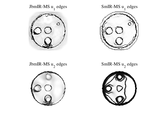
Figure 6: Reconstructed edge images.

7.4.2 Example 2

For JbmIR-MS we choose $\alpha_{1}=8.8\times 10^{3},\leavevmode\nobreak\ \beta_{1}=1.9\times 10^{-3},\leavevmode\nobreak\ \gamma_{1}=9.8,\leavevmode\nobreak\ \alpha_{2}=1\times 10^{5},\leavevmode\nobreak\ \beta_{2}=7\times 10^{-5},\leavevmode\nobreak\ \gamma_{2}=5$. For SmIR-MS XCT, we set $\alpha=8.8\times 10^{3},\leavevmode\nobreak\ \beta=8\times 10^{-3}.$ For SmIR-MS DOT, we set $\alpha=1\times 10^{5},\leavevmode\nobreak\ \beta=5\times 10^{-7}.$ The reconstructed results are shown in Figure 7. The image quality of reconstructed $u_{1}$ is improved using JbmIR-MS (SSIM from 0.75 to 0.86). The image quality of reconstructed $u_{2}$ is higher using JbmIR-MS (SSIM$=0.70$) then SmIR-MS (SSIM$=0.61$). The improvement in DOT image quality is greater than the first example because there are more similar parts between phantoms of two modalities in this example.

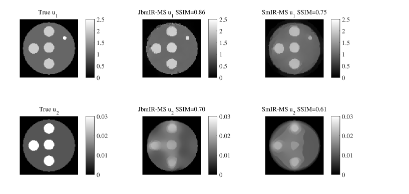
Figure 7: Phantom 2 reconstruction results. (top) The XCT phantom and reconstruction results, (bottom) The DOT phantom and reconstruction results. For SmIR-MS $u_{1}$ we have SSIM$=0.75$, and for JbmIR-MS $u_{1}$ we have SSIM$=0.86$, For SmIR-MS $u_{2}$ we have SSIM$=0.61$, for JbmIR-MS $u_{2}$ we have SSIM$=0.70$.

The edge information is shown in Figure 8. We can see that the edge information obtained from JbmIR-MS is clearer then SmIR-MS. Compare to the edge results in Example 1, the edge of the top circle for DOT image is much more distinct because the XCT phantom in this example can provide the edge information of the top circle.

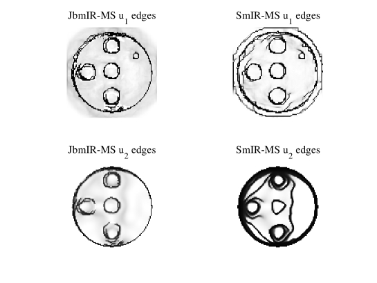
Figure 8: Reconstructed edge images

7.4.3 Example 3

For JbmIR-MS we choose $\alpha_{1}=8.8\times 10^{3},\leavevmode\nobreak\ \beta_{1}=1.9\times 10^{-3},\leavevmode\nobreak\ \gamma_{1}=9.8,\leavevmode\nobreak\ \alpha_{2}=1\times 10^{5},\leavevmode\nobreak\ \beta_{2}=6\times 10^{-5},\leavevmode\nobreak\ \gamma_{2}=5$. For SmIR-MS XCT, we choose $\alpha=8.8\times 10^{3},\leavevmode\nobreak\ \beta=8\times 10^{-3}.$ For SmIR-MS DOT, we choose $\alpha=1\times 10^{5},\leavevmode\nobreak\ \beta=5\times 10^{-7}.$ The reconstruction results are shown in Figure 9. According to the SSIM values, the image quality of reconstructed $u_{1}$ is improved using JbmIR-MS (SSIM from 0.76 to 0.87). The image quality of reconstructed $u_{2}$ is higher using JbmIR-MS (SSIM$=0.69$) then SmIR-MS (SSIM$=0.60$).

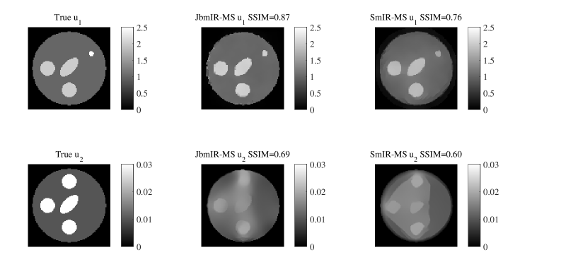
Figure 9: Phantom 3 reconstruction results. (top) The XCT phantom and reconstruction results, (bottom) The DOT phantom and reconstruction results. For SmIR-MS $u_{1}$ we have SSIM$=0.76$, and for JbmIR-MS $u_{1}$ we have SSIM$=0.87$, For SmIR-MS $u_{2}$ we have SSIM$=0.60$, for JbmIR-MS $u_{2}$ we have SSIM$=0.69$.

The edge information is illustrated in Figure 10. We can find that the middle ellipse shape for DOT is more obvious in JbmIR-MS edge result than in SmIR-MS edge result.

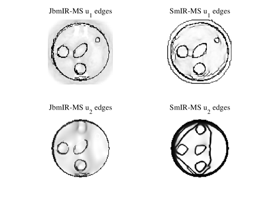
Figure 10: Reconstructed edge images

8 Discussion

In this work, we establish an image similarity measure in terms of image edges from Tversky’s theory of feature similarity in psychology to solve the DOT and XCT joint reconstruction problem. This similarity consists of Hausdorff measures of the common and different parts of image edges from both modalities. When applied to JbmIR it will improve the reconstructed image quality and will not force the nonexistent structures to be reconstructed.

To implement the joint reconstruction, a $\Gamma-$approximation(21) is proposed for the joint reconstruction functional. The current formulation of the $\Gamma$-approximation is based on the heuristics in [Page, 2015, § 4.5]. We are unable to prove the expected convergence mathematically, although a proof for $\gamma_{1}=\gamma_{2}=0$ might be possible by using the same method in [Page, 2015] where a lengthy proof for single modal image reconstruction with the extended Mumford-Shah function with a priori edge information is provided for $\gamma=0$. However, it is too tedious to reproduce such a proof in the current work and does not contribute any mathematical insight into this problem with such a stringent condition in our opinion. Instead, we concentrate in studying numerically how the proposed method can help improve the quality of reconstructed images in this work. In the $\Gamma$-approximation functional there isn’t any weighting parameters in front of the two fidelity terms, that is because they are independent of each other. We reconstruct the two modalities alternatively, and the information communication is achieved by edge similarity, so we just choose proper regularization parameters for penalty term to control the effect of the other modality and do not weight the fidelity term.

Since circle is the simplest shape, we first design phantoms with circle internal structure. For each example, the structure of the two phantoms are designed similar to each other. XCT should be able to reconstruct finer structure so we add a small circle to the XCT phantoms. DOT cannot distinguish such fine structure so we only design big circle inner structure. Considering that DOT can distinguish different soft tissue better than XCT, we add one more big circle in DOT phantom for Example 1 and Example 3. A reasonable similarity measure should maintain the distinctive structure in each modality and not force the nonexistent features in one modality to be reconstructed. In Example 2, the main parts are set exactly the same as each other to see if we can improve image quality more when the phantoms from two modalities share more common structure. And in Example 3, we change the shape of the middle structure to be an ellipse to see the performance of different methods for different shape of the inner structure.

Our JbmIR-MS is compared with SmIR-MS. From results shown in Figure 5 for Example 1, we can see that the quality of images reconstructed jointly is higher than that of images reconstructed under the SmIR-MS. The SSIM values increase $10.30\%$ and $12.78\%$ for DOT and XCT respectively. Looking at the reconstructed images, JbmIR-MS $u_{1}$ keeps the structure of the small circle and no extra top circle structure is reconstructed because of the information provided by $u_{2}$. As for JbmIR-MS $u_{2}$ the structure is more clear than SmIR-MS result especially the parts that are consistent with $u_{1}$. It is more obvious in the reconstructed edge information shown in Figure 6.

The results for Example 2 are shown in Figure 7. We can see that the image quality improvement is greater than that in Example 1. The SSIM values increase $14.85\%$ and $14.44\%$ for DOT and XCT respectively. We think that the reason that the enhancement in Example 2 is greater than that in Example 1 is because the phantoms of DOT and XCT modalities in Example 2 share more similar parts than Example 1, thus using our edge similarity measure, each modality can provide more a priori structural information. Compare to the edge results in Example 1, the edge of the top circle for DOT image is much sharper because the XCT phantom in this example can provide the edge information of the top circle.

In Example 3 we can see that for different shapes of the internal structure, ellipse in our case, JbmIR-MS method also provides better reconstructed images, shown in Figure 9. The SSIM values increase $13.82\%$ and $15.91\%$ for DOT and XCT respectively. And from the result figure we can clearly see the shape of the middle ellipse in our joint reconstruction result for DOT problem.

We find that the visual improvement of XCT reconstruction is not impressive, because the phantoms are easy for XCT. However, looking at their line profiles, the improvement is easy to capture as shown in Figures 11(a), 11(b) and 11(c). It can be seen that the XCT results using JbmIR-MS are closer to the true distributions than that using SmIR-MS.

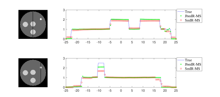
(a) XCT profiles for Phantom 1.

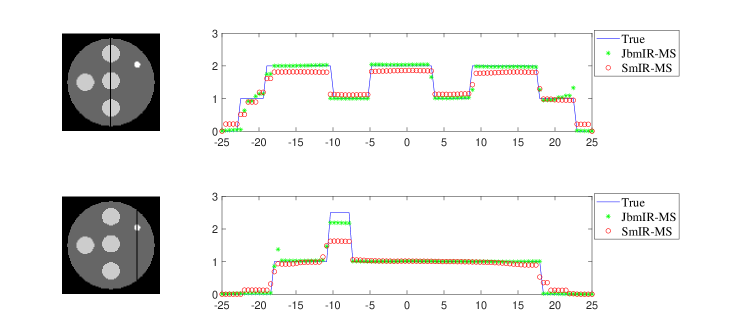
(b) XCT profiles for Phantom 2.

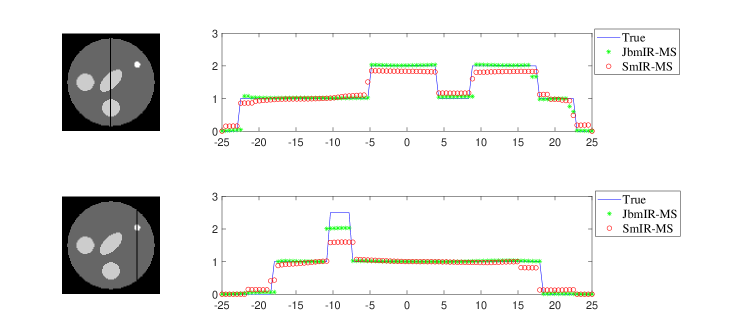
(c) XCT profiles for Phantom 3.

Figure 11: XCT profiles for the three phantoms and reconstructed images. Black vertical lines on images on the left-side show the positions of lines to draw the line profiles on the right-side. For the line profiles, the blue line shows absorption values of the truth image, red circles shows absorption values from the SmIR-MS of XCT, and green stars shows absorption values from the JbmIR-MS of XCT. It can be seen that the results from the JbmIR-MS are closer to the truth distributions than the SmIR-MS.

From the numerical results we can see that minimizing the Mumford-Shah functional enables us to reconstruct images and obtain edges at the same time. Since the images from two modalities share similar structure, our JbmIR-MS method adding the edge similarity measure to the Mumford-Shah functional implements the information communication between DOT and XCT modalities which helps to enhance the reconstructed image quality for both modalities. With proper choice of regularization parameters, our similarity measure is able to help enhancing the image quality of the common features, to remain distinctive features for each modality and not force to reconstruct the nonexistent features. The smoothing term together with the usage of separate edge variables to represent structure information enable us to get piecewise smooth reconstructed images with clear and sharp edge with noise data. However there are a number of parameters, including regularization parameters, needed to be chosen carefully and the current parameter choosing is a trial-error approach. For 3D situation, the DOT/XCT bi-modal imaging system has already been set up. We are now preparing the optical phantoms [He et al., 2018] for real physical experiment. And we are going to test the JbmIR-MS method with realistic data acquired under our bi-modal imaging system.

9 Conclusion

In this paper, we have proposed an asymmetric edge similarity measure following the feature contrast model in [Tversky, 1977] to solve the DOT and XCT joint reconstruction problem. This edge similarity measure is able to implement the information communication between the two modalities, thus improves the reconstructed image quality for both modalities. Meanwhile, it remains distinctive structure for each modality and does not force the nonexistent edges to be reconstructed when some of the structures only exist in one modality.

Representing the edge sets by edge indicator functions, a $\Gamma$-approximation (21) is proposed to make it easier to implement the joint reconstruction. To demonstrate the performance of our JbmIR-MS algorithm, we have designed two dimensional numerical phantoms and calculate the minimizers of the $\Gamma$-approximation. To calculate the minimizers, we use gradient descent method with the negative gradient as the descent direction and the step size chosen by backtracking line search with the Armijo-Goldstein stopping condition.

We have evaluated the reconstructed images using SSIM value with the corresponding ground truth as reference image. We compared our JbmIR-MS method with SmIR-MS which shows that joint reconstruction can provide better quality images and clearer edge information.

The results in this work show the effectiveness of the reconstruction method using Mumford-Shah functional with proposed edge similarity measure in 2D.

References

References

- [Armijo, 1966] Armijo, L. (1966). Minimization of functions having Lipschitz continuous first partial derivatives. Pacific Journal of Mathematics, 16(1):1–3.
- [Arridge, 1999] Arridge, S. R. (1999). Optical tomography in medical imaging. Inverse problems, 15(2):R41.
- [Arridge and Schotland, 2009] Arridge, S. R. and Schotland, J. C. (2009). Optical tomography: forward and inverse problems. Inverse Problems, 25(12):123010.
- [Baikejiang et al., 2017] Baikejiang, R., Zhang, W., and Li, C. Q. (2017). Diffuse optical tomography for breast cancer imaging guided by computed tomography: A feasibility study. Journal of X-Ray Science and Technology, 25(3):341–355.
- [Biasotti et al., 2016] Biasotti, S., Cerri, A., Bronstein, A., and Bronstein, M. (2016). Recent trends, applications, and perspectives in 3d shape similarity assessment. Computer Graphics Forum, 35(6):87–119.
- [Blough, 2001] Blough, D. S. (2001). The perception of similarity. In Cook, R. B., editor, Avian Visual Cognition. https://pigeon.psy.tufts.edu/avc/dblough/default.htm.
- [Boas, 2014] Boas, D. (2014). Digital breast tomosynthesis guided tomographic optical breast imaging (TOBI). Clinical trials 2014 - 2019, https://clinicaltrials.gov/ct2/show/NCT02033486.
- [Bockisch et al., 2009] Bockisch, A., Freudenberg, L. S., Schmidt, D., and Kuwert, T. (2009). Hybrid imaging by SPECT/CT and PET/CT: Proven outcomes in cancer imaging. Seminars in Nuclear Medicine, 39(4):276–289.
- [Bowsher et al., 1996] Bowsher, J. E., Johnson, V. E., Turkington, T. G., Jaszczak, R. J., Floyd, C., and Coleman, R. E. (1996). Bayesian reconstruction and use of anatomical a priori information for emission tomography. IEEE Transactions on Medical Imaging, 15(5):673–686.
- [Bowsher et al., 2004] Bowsher, J. E., Yuan, H., Hedlund, L. W., Turkington, T. G., Akabani, G., Badea, A., Kurylo, W. C., Wheeler, C. T., Cofer, G. P., Dewhirst, M. W., and Johnson, G. A. (2004). Utilizing MRI information to estimate F18-FDG distributions in rat flank tumors. In Seibert, J. A., editor, 2004 IEEE Nuclear Science Symposium Conference Record, Vols 1-7, IEEE Nuclear Science Symposium - Conference Record, pages 2488–2492.
- [Brooksby et al., 2005] Brooksby, B., Jiang, S. D., Dehghani, H., Pogue, B. W., Paulsen, K. D., Weaver, J., Kogel, C., and Poplack, S. P. (2005). Combining near-infrared tomography resonance imaging to study in vivo and magnetic breast tissue: implementation of a laplacian-type regularization to incorporate magnetic resonance structure. Journal of Biomedical Optics, 10(5):10.
- [Brooksby et al., 2006] Brooksby, B., Pogue, B. W., Jiang, S. D., Dehghani, H., Srinivasan, S., Kogel, C., Tosteson, T. D., Weaver, J., Poplack, S. P., and Paulsen, K. D. (2006). Imaging breast adipose and fibroglandular tissue molecular signatures by using hybrid mri-guided near-infrared spectral tomography. Proceedings of the National Academy of Sciences of the United States of America, 103(23):8828–8833.
- [Canny, 1986] Canny, J. (1986). A computational approach to edge detection. IEEE Transactions on Pattern Analysis and Machine Intelligence, 8(6):679 – 698.
- [Catana, 2017] Catana, C. (2017). Principles of simultaneous PET/MR imaging. Magnetic Resonance Imaging Clinics of North America, 25(2):231–+.
- [Censor et al., 2008] Censor, Y., Jiang, M., and Louis, A. K. (2008). Mathematical Methods in Biomedical Imaging and Intensity-modulated Radiation Therapy (IMRT). Scuola Normale Superiore Edizioni della Normale.
- [Chan et al., 2009] Chan, C., Fulton, R., Feng, D. D., and Meikle, S. (2009). Regularized image reconstruction with an anatomically adaptive prior for positron emission tomography. Physics in Medicine and Biology, 54(24):7379–7400.
- [Cherry, 2009] Cherry, S. R. (2009). Multimodality imaging: Beyond PET/CT and SPECT/CT. Seminars in Nuclear Medicine, 39(5):348–353.
- [Delbeke et al., 2009] Delbeke, D., Schoder, H., Martin, W. H., and Wahl, R. L. (2009). Hybrid imaging (SPECT/CT and PET/CT): Improving therapeutic decisions. Seminars in Nuclear Medicine, 39(5):308–340.
- [Deng et al., 2015] Deng, B., Brooks, D. H., Boas, D. A., Lundqvist, M., and Fang, Q. Q. (2015). Characterization of structural-prior guided optical tomography using realistic breast models derived from dual-energy x-ray mammography. Biomedical Optics Express, 6(7):2366–2379.
- [Dewaraja et al., 2010] Dewaraja, Y. K., Koral, K. F., and Fessler, J. A. (2010). Regularized reconstruction in quantitative SPECT using CT side information from hybrid imaging. Physics in Medicine and Biology, 55(9):2523–2539.
- [Douiri et al., 2007] Douiri, A., Schweiger, M., Riley, J., and Arridge, S. R. (2007). Anisotropic diffusion regularization methods for diffuse optical tomography using edge prior information. Measurement Science and Technology, 18(1):87–95.
- [Ehrhardt, 2015] Ehrhardt, M. J. (2015). Joint Reconstruction for Multi-Modality Imaging with Common Structure. PhD thesis, University College London.
- [Ehrhardt et al., 2015] Ehrhardt, M. J., Thielemans, K., Pizarro, L., Atkinson, D., Ourselin, S., Hutton, B. F., and Arridge, S. R. (2015). Joint reconstruction of PET-MRI by exploiting structural similarity. Inverse Problems, 31(1):015001.
- [Even-Sapir et al., 2009] Even-Sapir, E., Keidar, Z., and Bar-Shalom, R. (2009). Hybrid imaging (SPECT/CT and PET/CT)-improving the diagnostic accuracy of functional/metabolic and anatomic imaging. Seminars in Nuclear Medicine, 39(4):264–275.
- [Fang et al., 2010] Fang, Q. Q., Moore, R. H., Kopans, D. B., and Boas, D. A. (2010). Compositional-prior-guided image reconstruction algorithm for multi-modality imaging. Biomedical Optics Express, 1(1):223–235.
- [Fessler et al., 1992] Fessler, J. A., Clinthorne, N. H., and Rogers, W. L. (1992). Regularized emission image-reconstruction using imperfect side information. IEEE Transactions on Nuclear Science, 39(5):1464–1471.
- [Gallardo, 2007] Gallardo, L. A. (2007). Multiple cross-gradient joint inversion for geospectral imaging. Geophysical Research Letters, 34(19).
- [Gallardo and Meju, 2011] Gallardo, L. A. and Meju, M. A. (2011). Structure-coupled multiphysics imaging in geophysical sciences. Reviews of Geophysics, 49(1).
- [Geman and Geman, 1984] Geman, S. and Geman, D. (1984). Stochastic relaxation, gibbs distributions, and the bayesian restoration of images. IEEE Transactions on Pattern Analysis and Machine Intelligence, 6:721–741.
- [Gindi et al., 1993] Gindi, G., Lee, M., Rangarajan, A., and Zubal, I. G. (1993). Bayesian reconstruction of functional images using anatomical information as priors. IEEE Transactions on Medical Imaging, 12(4):670–680.
- [Haber and Gazit, 2013] Haber, E. and Gazit, M. H. (2013). Model fusion and joint inversion. Surveys in Geophysics, 34(5):675–695.
- [Haber and Oldenburg, 1997] Haber, E. and Oldenburg, D. (1997). Joint inversion: a structural approach. Inverse Problems, 13(1):63.
- [He et al., 2018] He, D., He, J., and Mao, H. (2018). Phantom preparation and optical property determination. Sensing and Imaging, 19(1):10.
- [Jiang et al., 2014] Jiang, M., Maass, P., and Page, T. (2014). Regularizing properties of the Mumford–Shah functional for imaging applications. Inverse Problems, 30(3):035007.
- [Judenhofer et al., 2008] Judenhofer, M. S., Wehrl, H. F., Newport, D. F., Catana, C., Siegel, S. B., Becker, M., Thielscher, A., Kneilling, M., Lichy, M. P., Eichner, M., Klingel, K., Reischl, G., Widmaier, S., Rocken, M., Nutt, R. E., Machulla, H. J., Uludag, K., Cherry, S. R., Claussen, C. D., and Pichler, B. J. (2008). Simultaneous PET-MRI: a new approach for functional and morphological imaging. Nature Medicine, 14(4):459–465.
- [Kaufmann and Di Carli, 2009] Kaufmann, P. A. and Di Carli, M. F. (2009). Hybrid SPECT/CT and PET/CT imaging: The next step in noninvasive cardiac imaging. Seminars in Nuclear Medicine, 39(5):341–347.
- [Kazantsev et al., 2012] Kazantsev, D., Simon, R. A., Pedemonte, S., Bousse, A., Erlandsson, K., Hutton, B. F., and Ourselin, S. (2012). An anatomically driven anisotropic diffusion filtering method for 3D SPECT reconstruction. Physics in Medicine & Biology, 57(12):3793.
- [Klann et al., 2011] Klann, E., Ramlau, R., and Ring, W. (2011). A Mumford-Shah level-set approach for the inversion and segmentation of SPECT/CT data. Inverse Problems & Imaging, 5(1):137–166.
- [Knoll et al., 2017] Knoll, F., Holler, M., Koesters, T., Otazo, R., Bredies, K., and Sodickson, D. K. (2017). Joint MR-PET reconstruction using a multi-channel image regularizer. IEEE transactions on medical imaging, 36(1):1–16.
- [Leahy and Yan, 1991] Leahy, R. and Yan, X. (1991). Incorporation of anatomical MR data for improved functional imaging with PET. In Information Processing in Medical imaging, pages 105–120. Springer.
- [Louis, 1989] Louis, A. K. (1989). Inverse und schlecht gestellte Probleme. Teubner.
- [Louis, 2011] Louis, A. K. (2011). Feature reconstruction in inverse problems. Inverse Problems, 27(6):065010.
- [Marr, 1982] Marr, D. (1982). Vision. Freeman.
- [Marr and Hildreth, 1980] Marr, D. and Hildreth, E. (1980). Theory of edge detection. Proceedings of the Royal Society of London. Series B, 207:187 – 217.
- [Mumford, 1991] Mumford, D. (1991). Mathematical theories of shape: do they model perception? Proc.SPIE, 1570:1570 – 1570 – 9.
- [Mumford and Shah, 1989] Mumford, D. and Shah, J. (1989). Optimal approximations by piecewise smooth functions and associated variational problems. Communications on Pure and Applied Mathematics, 42(5):577–685.
- [Natterer, 2001] Natterer, F. (2001). The Mathematics of Computerized Tomography. SIAM.
- [Natterer et al., 2002] Natterer, F., Wubbeling, F., and Wang, G. (2002). Mathematical methods in image reconstruction. Medical Physics, 29(1):107–108.
- [Nuyts, 2007] Nuyts, J. (2007). The use of mutual information and joint entropy for anatomical priors in emission tomography. In 2007 IEEE Nuclear Science Symposium, IEEE Nuclear Science Symposium, pages 4149–4154. IEEE Press.
- [Ouyang et al., 1994] Ouyang, X., Wong, W. H., Johnson, V. E., Hu, X., and Chen, C.-T. (1994). Incorporation of correlated structural images in PET image reconstruction. IEEE Transactions on Medical Imaging, 13(4):627–640.
- [Page, 2015] Page, T. S. (2015). Image reconstruction by Mumford-Shah regularization with a priori edge information. PhD thesis, Universität Bremen.
- [Panagiotou et al., 2009] Panagiotou, C., Somayajula, S., Gibson, A. P., Schweiger, M., Leahy, R. M., and Arridge, S. R. (2009). Information theoretic regularization in diffuse optical tomography. JOSA A, 26(5):1277–1290.
- [Perona and Malik, 1990] Perona, P. and Malik, J. (1990). Scale-space and edge detection using anisotropic diffusion. IEEE Transactions on Pattern Analysis and Machine Intelligence, 12(7):629 – 639.
- [Ramlau and Ring, 2007] Ramlau, R. and Ring, W. (2007). A Mumford–Shah level-set approach for the inversion and segmentation of X-ray tomography data. Journal of Computational Physics, 221(2):539–557.
- [Rasch et al., 2017] Rasch, J., Brinkmann, E.-M., and Burger, M. (2017). Joint reconstruction via coupled bregman iterations with applications to PET-MR imaging. Inverse Problems, 34(1):014001.
- [Rigie and La Riviere, 2015] Rigie, D. S. and La Riviere, P. J. (2015). Joint reconstruction of multi-channel, spectral ct data via constrained total nuclear variation minimization. Physics in Medicine and Biology, 60(5):1741–1762.
- [Rondi, 2008] Rondi, L. (2008). Reconstruction in the inverse crack problem by variational methods. European Journal of Applied Mathematics, 19(6):635–660.
- [Rondi and Santosa, 2001] Rondi, L. and Santosa, F. (2001). Enhanced electrical impedance tomography via the Mumford–Shah functional. ESAIM: Control, Optimisation and Calculus of Variations, 6:517–538.
- [Rorissa, 2007] Rorissa, A. (2007). Relationships between perceived features and similarity of images: A test of tversky’s contrast model. Journal of the American Society for Information Science & Technology, 58(10):1401–1418.
- [Rudin et al., 1992] Rudin, L. I., Osher, S., and Fatemi, E. (1992). Nonlinear total variation based noise removal algorithms. Physica D, 60:259 – 268.
- [Santini and Jain, 1997] Santini, S. and Jain, R. (1997). Similarity is a geometer. Multimedia Tools and Applications, 5(3):277–306.
- [Santini and Jain, 1999] Santini, S. and Jain, R. (1999). Similarity measures. IEEE Transactions on Pattern Analysis and Machine Intelligence, 21(9):871–883.
- [Sastry and Carson, 1997] Sastry, S. and Carson, R. E. (1997). Multimodality bayesian algorithm for image reconstruction in positron emission tomography: a tissue composition model. IEEE Transactions on Medical imaging, 16(6):750–761.
- [Scherzer, 2010] Scherzer, O. (2010). Handbook of Mathematical Methods in Imaging. Springer Science & Business Media.
- [Schramm et al., 2018] Schramm, G., Holler, M., Rezaei, A., Vunckx, K., Knoll, F., Bredies, K., Boada, F., and Nuyts, J. (2018). Evaluation of parallel level sets and bowsher’s method as segmentation- free anatomical priors for time-of-flight pet reconstruction. IEEE Transactions on Medical Imaging, 37(2):590–603.
- [Schweiger and Arridge, 2014] Schweiger, M. and Arridge, S. R. (2014). The Toast++ software suite for forward and inverse modeling in optical tomography. Journal of Biomedical Optics, 19(4):040801.
- [Skopal and Bustos, 2011] Skopal, T. and Bustos, B. (2011). On nonmetric similarity search problems in complex domains. ACM Computing Surveys, 43(4).
- [Somayajula et al., 2011] Somayajula, S., Panagiotou, C., Rangarajan, A., Li, Q. Z., Arridge, S. R., and Leahy, R. M. (2011). PET image reconstruction using information theoretic anatomical priors. IEEE Transactions on Medical Imaging, 30(3):537–549.
- [Steiner, 2007] Steiner, G. (2007). Application and data fusion of different sensor modalities in tomographic imaging. Elektrotechnik und Informationstechnik, 124(7):232–239.
- [Tang and Rahmim, 2009] Tang, J. and Rahmim, A. (2009). Bayesian pet image reconstruction incorporating anato-functional joint entropy. Physics in Medicine and Biology, 54(23):7063–7075.
- [Townsend, 2008] Townsend, D. W. (2008). Multimodality imaging of structure and function. Physics in Medicine and Biology, 53(4):R1–R39.
- [Tversky, 1977] Tversky, A. (1977). Features of similarity. Psychological review, 84(4):327.
- [Tversky and Gati, 1982] Tversky, A. and Gati, I. (1982). Similarity, separability, and the triangle inequality. Psychological Review, 89(2):123.
- [Wang et al., 2015] Wang, G., Kalra, M., Murugan, V., Xi, Y., Gjesteby, L., Getzin, M., Yang, Q. S., Cong, W. X., and Vannier, M. (2015). Vision 20/20: Simultaneous CT-MRI - next chapter of multimodality imaging. Medical Physics, 42(10):5879–5889.
- [Wang et al., 2012] Wang, G., Zhang, J., Gao, H., Weir, V., Yu, H. Y., Cong, W. X., Xu, X. C., Shen, H. O., Bennett, J., Furth, M., Wang, Y., and Vannier, M. (2012). Towards omni-tomography — grand fusion of multiple modalities for simultaneous interior tomography. Plos One, 7(6).
- [Wang et al., 2004] Wang, Z., Bovik, A. C., Sheikh, H. R., and Simoncelli, E. P. (2004). Image quality assessment: from error visibility to structural similarity. IEEE transactions on image processing, 13(4):600–612.
- [Weizman et al., 2016] Weizman, L., Eldar, Y. C., and Ben Bashat, D. (2016). Reference-based MRI. Medical Physics, 43(10):5357–5369.
- [Wikipedia contributors, 2017] Wikipedia contributors (2017). Backtracking line search — Wikipedia, the free encyclopedia. [Online; accessed 20-May-2018].
- [Yalavarthy et al., 2007] Yalavarthy, P. K., Pogue, B. W., Dehghani, H., Carpenter, C. M., Jiang, S. D., and Paulsen, K. D. (2007). Structural information within regularization matrices improves near infrared diffuse optical tomography. Optics Express, 15(13):8043–8058.
- [Yang et al., 2015] Yang, Y. D., Wang, K. K. H., Eslami, S., Iordachita, I., Patterson, M. S., and Wong, J. W. (2015). Systematic calibration of an integrated x-ray and optical tomography system for preclinical radiation research. Medical Physics, 42(4):1710–1720.
- [Yuan et al., 2010] Yuan, Z., Zhang, Q., Sobel, E. S., and Jiang, H. (2010). High-resolution X-ray guided three-dimensional diffuse optical tomography of joint tissues in hand osteoarthritis: Morphological and functional assessments. Medical physics, 37(8):4343–4354.
- [Zhang et al., 1994] Zhang, Y., Fessler, J. A., Clinthorne, N. H., and Rogers, W. L. (1994). Joint estimation for incorporating MRI anatomic images into SPECT reconstruction. Nuclear Science Symposium and Medical Imaging Conference. IEEE Press.