Distribution of $S$-matrix poles for one-dimensional disordered wires

Abstract

By the use of the effective non-Hermitian Hamiltonian approach to scattering we study the distribution of the scattering matrix ($S$-matrix) poles in one-dimensional (1D) models with various types of diagonal disorder. We consider the case of 1D tight-binding wires, with both on-site uncorrelated and correlated disorder, coupled to the continuum through leads attached to the wire edges. In particular, we focus on the location of the $S$-matrix poles in the complex plane as a function of the coupling strength and the disorder strength. Specific interest is paid to the super-radiance transition emerging at the perfect coupling between wire and leads. We also study the effects of correlations intentionally imposed to the wire disorder.

I Introduction

To date, the paradigmatic one-dimensional (1D) Anderson model with white-noise diagonal disorder has been rigorously studied in great detail. The main result is that all eigenstates are exponentially localized in the infinite geometry, characterized by the amplitude decrease with the distance from their centers. The characteristic scale on which they are effectively localized is known as the localization length $L_{\mbox{\scriptsize{loc}}}$ which can be easily computed numerically in the frame of the transfer matrix method (see Ref. IKM12 and references therein). This energy-dependent length is of utmost importance due to the single parameter scaling, according to which all transport properties of the finite wires are explicitly defined by the ratio $L_{\mbox{\scriptsize{loc}}}/N$, where $N$ is the length of the wire (see, for instance, Ref. LGP88 ). Specifically, there are various rigorous approaches allowing to derive the distribution function for the transmission coefficient characterizing the scattering process through finite wires of size $N$ (for references, see M99 ).

Complimentary to the transfer matrix method, the scattering properties of electromagnetic waves propagating through finite wires can also be studied via the scattering matrix ($S$-matrix). There is an enormous number of papers devoted to the theory of the $S$-matrix in application to complex physical systems such as heavy nuclei, many-electron atoms, and quantum dots. Assuming a quite complex (chaotic) behavior of the closed (isolated) systems, it was suggested that various types of random matrices can serve as good mathematical models in describing statistical properties of scattering. In particular, typical models are represented by non-Hermitian matrices with a real part in terms of a fully random matrix plus an imaginary part of certain structure absorbing the details of the coupling to the continuum. In this way many results both analytical and numerical, have been obtained during the last decades (see, for example, Refs. MW69 ; supersym ; SZ92 and references therein).

One important question in scattering theory is about the type of distribution of the widths of resonances, emerging in the transmission coefficient as a function of the energy. For sufficiently week coupling to the continuum (slightly open systems) the resonances are well isolated from each other; a situation termed as isolated resonances. This happens when the resonance widths are smaller than the spacings between the locations of resonances. A completely different situation arises when the widths of the resonances are much larger than the spacing between them. In this case the resonances are strongly overlapped, thus resulting in specific properties of scattering. For random matrix models it was shown that the crossover from isolated to overlapped resonances is quite sharp in dependence on the coupling strength $\gamma$, and at the transition point the mean value of the resonances diverges. With the increase of $\gamma$ towards strongly overlapped resonances, a remarkable effect emerges, known as superradiance SZ92 . In this regime a finite number of resonances have very large widths while the other resonances begin to be more and more narrow with the increase of the coupling.

The goal of this paper is to study the 1D Anderson model with both white-noise disorder and correlated disorder, focusing on the pole distribution in dependence of the degree of localization of eigenstates and of the strength of the coupling to the continuum. Although this model is very different from random matrix models, we expect that some of the properties, such as the superradiant transition and the divergence of the resonance widths at the superradiant transition point, develop similarly to those in random matrix theory (RMT) models. The distinctive property of our model is that by increasing the disorder one can change the degree of localization of eigenstates in the closed wires, therefore, in the wires attached to the leads the localization effects may greatly affect the pole distribution. Another issue to address is how correlations imposed to the diagonal disorder modify the pole distribution at the mobility edges emerging due to specific long-range correlations. We hope that our numerical results can help to develop an analytical approach to the problem of scattering in 1D wires in the case when a closed system is strongly influenced by localization effects.

II The Model and Scattering setup

The 1D Anderson model is defined by the stationary Schrödinger equation

$$\psi_{n+1}+\psi_{n-1}+\epsilon_{n}\psi_{n}=E\psi_{n}\ .$$ (1)

for the electron wave function $\psi_{n}$ of energy $E$. In what follows we consider both uncorrelated and correlated disorder specified by the site potentials $\epsilon_{n}$. The energies $E$ and $\epsilon_{n}$ are dimensionless quantities measured in units of the kinetic electron energy.

In the non-disordered case ($\epsilon_{n}=0$), the solutions $\psi_{n}$ are plane waves with wave number $\mu$ defining the dispersion relation

$$E=2\cos\mu\ ,\quad 0\leq\mu\leq\pi\ .$$ (2)

For the the disordered case we assume that the distribution of on-site energies $\epsilon_{n}$ is characterized by random variables with zero mean and variance $\sigma^{2}$,

$$\langle\epsilon_{n}\rangle=0\ ,\quad\langle\epsilon^{2}_{n}\rangle=\sigma^{2}\ .$$

Here $\langle\dots\rangle$ stands for the average over disorder realizations. We also assume that the disorder is weak,

$$\sigma^{2}\ll 1\ ,$$ (3)

which is needed to develop a proper perturbation theory.

In the case of uncorrelated disorder all electron eigenstates are exponentially localized with the characteristic length $L_{\mbox{\scriptsize{loc}}}$ in the limit of infinite wire length ($N\rightarrow\infty$). As is known, for white-noise disorder the localization length $L_{\mbox{\scriptsize{loc}}}$ is given by the Thouless expression T79 (see also Ref. IKM12 ),

$$L^{-1}_{\mbox{\scriptsize{loc}}}=\frac{\sigma^{2}}{8\sin^{2}\mu}=\frac{w^{2}}{96(1-E^{2}/4)}\ .$$ (4)

Here $\mu$ is defined through the dispersion relation (2) and the second relation is given for a box distribution of $\epsilon_{n}$ specified by the interval $[-w/2,w/2]$.

Below we study 1D finite wires of size $N$ with disordered on-site potentials $\epsilon_{n}$. The first and last sites of the disordered lattice are connected to semi-infinite ideal leads through coupling amplitudes $\sqrt{\gamma}$. In this way the leads are considered as a continuum to which the disordered wire is coupled according to given boundary conditions. The scattering properties of such open system can be formulated in terms of the non-Hermitian Hamiltonian MW69 ; SZ92 . The key point of this approach is based on the projection of the total Hermitian Hamiltonian (disordered wire plus leads) onto the basis defined by the Hamiltonian $H$ describing the properties of the closed model (the disordered wire only).

In our model, the non-Hermitian Hamiltonian has the following form near the band center ($E=0$) SIZC12 :

$${\cal H}_{mn}=H_{mn}-\frac{i}{2}W_{mn}$$ (5)

with

$$W_{mn}=2\pi\sum_{c=L,R}A^{(c)}_{m}A^{(c)}_{n}\ ,$$ (6)

where $W_{mn}$ is defined by the coupling amplitudes

$$A^{L,R}_{i}=\sqrt{\frac{\gamma}{\pi}}\left(\delta^{(L)}_{i1}+\delta^{(R)}_{iN}\right)\ .$$ (7)

Here, $H_{mn}$ is the Hamiltonian of the 1D Anderson model

$$H_{nm}=\epsilon_{n}\delta_{mn}+\delta_{m,n+1}+\delta_{m,n-1}\ ,$$ (8)

while the non-Hermitian part $W$ is given in terms of the coupling amplitudes $A^{(c)}_{i}$ between the internal states $|i\rangle$ and open decay channels $c=L,R$, where $L$ and $R$ stand for left and right, respectively.

With the non-Hermitian Hamiltonian, it is possible to obtain the scattering matrix $S$ in the form,

$$S=\frac{1-iK}{1+iK}\ ,$$ (9)

where the reaction matrix $K$ is given by

$$K^{ab}=\sum_{j}\frac{C^{(a)}_{j}C^{(b)}_{j}}{E-E_{j}},\ \ C^{(c)}_{j}=\sum_{m}A^{(c)}_{m}\psi^{(j)}_{m}\ ,$$ (10)

and $\psi^{(j)}_{m}$ is the $m$ component of the $j$-th eigenstate of the closed Hamiltonian (8) with eigenvalues $E_{j}$.

One of the quantities studied in this work is the distribution of the eigenvalues

$$\Omega_{k}=\omega_{k}-\frac{i}{2}\Gamma_{k}$$ (11)

of the non-Hermitian Hamiltonian (5); here $\omega_{k}$ and $\Gamma_{k}$ are called the position and the width of the $k-$resonance, respectively. The eigenvalues $\Omega_{k}$ can also be treated as the poles of the $S$-matrix, since one can write

$$S(E)=1-2\pi iA^{T}(E)\frac{1}{E-{\cal H}}A(E)\ ,$$

where $A(E)$ is the $N\times 2$ matrix with columns composed by the coupling amplitudes $A^{(c)}_{i}$.

In general the poles of the $S$-matrix for the 1D Anderson model depend on three parameters: the energy $E$, the coupling constant $\gamma$, and the localization length $L_{\mbox{\scriptsize{loc}}}$ (given by Eq. (4)). However, without loss of generality, in this work we fix the energy to $E=0$. It is known that depending on the ratio between the localization length and the system size $N$, there are three different regimes for the scattering processes: the ballistic regime characterized by $L_{\mbox{\scriptsize{loc}}}\gg N$, the chaotic regime where $L_{\mbox{\scriptsize{loc}}}\approx N$, and the localized regime which occurs for $L_{\mbox{\scriptsize{loc}}}\ll N$ (see for example Ref. IKM12 ).

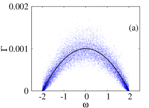
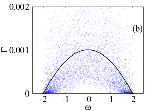
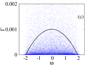
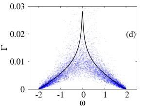
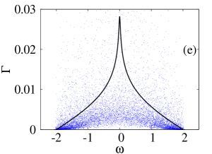
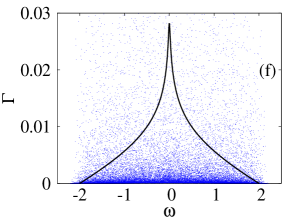
Figure 1: Imaginary vs. real part of the $S$-matrix poles $\Omega$ [see Eq. (11)] for 1D disordered wires of length $N=800$ coupled to the continuum with strength $\gamma=0.1$ (upper panels) and $\gamma=1$ (lower panels). The disorder strength was set to $\sigma^{2}=0.001$, $L_{\mbox{\scriptsize{loc}}}/N=10$ (left panels); $\sigma^{2}=0.01$, $L_{\mbox{\scriptsize{loc}}}/N=1$ (middle panels); and $\sigma^{2}=0.1$, $L_{\mbox{\scriptsize{loc}}}/N=0.1$ (right panels). Black curves represent the corresponding non-disordered wires. Here, 50 wire realizations were used.

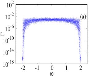
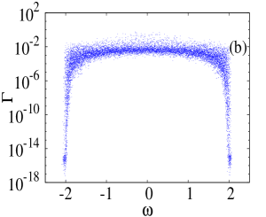
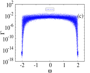
Figure 2: Imaginary vs. real part of the $S$-matrix poles $\Omega$ [see Eq. (11)] for 1D disordered wires of length $N=800$ coupled to the continuum with (a) $\gamma=0.1$, (b) $\gamma=1$, and (c) $\gamma=1.5$. The disorder strength was set to $\sigma^{2}=0.01$ such that $L_{\mbox{\scriptsize{loc}}}/N=1$. Here, 50 wire realizations were used. The small rectangle in (c) encloses the superradiant states.

III $S$-matrix poles: White-noise disorder

In this Section we consider the case of uncorrelated disorder: $\langle\epsilon_{n}\epsilon_{n+m}\rangle=0$, for $m\neq 0$. First, in Fig. 1 we report the $S$-matrix poles as the localization length decreases (from left to right) for two different values of the coupling strength: $\gamma=0.1$ (upper panels) and $\gamma=1$ (lower panels). In the ballistic regime, $L_{\mbox{\scriptsize{loc}}}\gg N$, see Fig. 1(left panels), the poles are distributed around the curves corresponding to the non-disordered case, which are shown as continuous black curves in all panels of Fig. 1. This behavior is easy to understand since the eigenstates of the disordered wires in this regime remain close to the eigenstates of wires with zero disorder (plane waves). In the chaotic regime, $L_{\mbox{\scriptsize{loc}}}\approx N$, the eigenstates are still extended (as in the ballistic regime), however, they produce strong fluctuations of $\Gamma$ values. As one can see by comparing Fig. 1(left and middle panels), the distribution of poles is quite sensitive to whether the eigenstates are quasi-regular or chaotic. Finally, for the localized regime, $L_{\mbox{\scriptsize{loc}}}\ll N$, only few eigenstates touch the wire boundaries and, as a consequence, the influence of the continuum is reduced producing a distribution of poles closer to the real axis, as Fig. 1(right panels) shows.

As the coupling parameter $\gamma$ increases, we observe the following effect. At zero coupling to the continuum the $S$-matrix poles are located along the real axis. As the coupling is turned on the poles acquire an imaginary part and, if the average width $\langle\Gamma\rangle$ is small as compared to the level spacing $D$ of the closed system, the cross sections in the scattering process reveal isolated resonances and the poles form a single cloud close to the real axis in the complex plane. However, with the increase of the coupling parameter $\gamma$, a crossover from isolated to overlapping resonances occurs; this crossover at $\gamma\approx 1$ is characterized by the appearance of two clouds of poles in the complex plane: one cloud corresponds to isolated resonances (with small $\Gamma$; $\Gamma\ll D$) and the other one to strongly overlapped ones (with large $\Gamma$; $\Gamma\gg D$). The latter states are termed superradiant states since they are short-lived, in contrast with long-lived states with small $\Gamma$. In the literature this segregation of poles is known as the superradiant transition. As we demonstrate below, the transition between isolated and superradiant states is very sharp with respect to the change of $\gamma$ and can be associated with a kind of phase transition.

Then, in Fig. 2 the aforementioned pole segregation is displayed. The lower cloud in Fig. 2(c) corresponds to $(N-2)N_{d}$ long-lived states, whereas the upper cloud (labeled by the small rectangle) represents $2N_{d}$ short-lived or superradiant states, being $N_{d}$ the number of realizations of the disorder (the factor 2 here accounts for the number of leads connected to the 1D wire). Notice that in this figure we show the superradiant transition for the chaotic regime $L_{\mbox{\scriptsize{loc}}}\approx N$ only, however, the existence of such transition and the value of $\gamma$ where it takes place do not depend on the degree of localization.

It is important to note that the control parameter determining the strength of the coupling to the continuum can be written as SIZC12

$$\kappa=\frac{2\pi\gamma}{ND}\ ,$$

where $D$ is the mean level spacing at the center of the energy band of the isolated wire. Note that $D$ can easily be evaluated if one takes into account the weak disorder condition (3). In this situation, the eigenvalues of the Hamiltonian (8) of the disordered wire are practically equal to the corresponding eigenvalues of the Hamiltonian (8) with $\epsilon_{n}=0$. Therefore, the dispersion relation (2) can be used. In addition, if fixed boundary conditions are imposed, the wave number takes the discrete values $\mu_{q}=q\pi/(N+1)$, with $q=1,\dots N$, and $D$ is then simply given by

$$D=\frac{2\pi}{N}\ .$$ (12)

Therefore, near to the band center $\kappa\approx\gamma$ and the superradiant transition takes place at $\kappa\approx 1$. It is quite interesting that the same critical value of $\kappa$ emerges also in other models such as the Gaussian Orthogonal Ensemble (GOE) of random matrices and two-body random interaction models brody81 ; TBRI . The superradiant transition in the 1D Anderson model has already been reported in the literature, see for example Refs. VZ05 ; celardo10 . In addition, the interplay between supperradiance and disorder has been previously established when all the sites of a lattice are coupled to a common decay channel CBKB13 . Also, the pole distribution, at perfect coupling, for the tree-dimensional Anderson model has been studied in WMK06 .

IV Mean value and fluctuations of resonance widths

In the previous Section, we made a qualitative description of the superradiant transition by analyzing the distribution of poles of the $S$-matrix in the complex plane. Now we focus on how the mean value of resonances (more precisely, the mean value of the imaginary part of the eigenvalues) depends on the strength of the coupling to continuum. This problem has been studied in detail for non-Hermitian Hamiltonians, see Eq. (5), in which the real part $H$ is a full random matrix belonging to one of standard ensembles (for example, to the GOE), and the imaginary part $W$ describes the coupling to continuum through a finite number of channels according to Eq. (6); see for example CIZB08 and references therein.

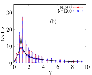
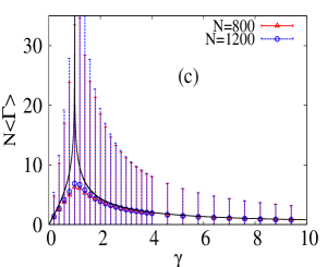
Figure 3: Average resonance width $\langle\Gamma\rangle$ at the band center as a function of the coupling to the continuum $\gamma$. Error bars are the corresponding standard deviation. (a) $L_{\mbox{\scriptsize{loc}}}/N=10$ (ballistic regime), (b) $L_{\mbox{\scriptsize{loc}}}/N=1$ (chaotic regime), and (c) $L_{\mbox{\scriptsize{loc}}}/N=0.1$ (localized regime). Circles and triangles represent different wire sizes. Black curves are Eq. (14). Here, 50 wire realizations were used.

One important analytical result, in the case of $M$ channels $c=1,...,M$, is that the mean width of the resonances reads FS96

$$\langle\Gamma\rangle=-\frac{MD}{2\pi}\ln\left(\frac{\tau-1}{\tau+1}\right),\ \ \tau=\frac{1}{2}\left(\gamma+\gamma^{-1}\right).$$ (13)

Here $D$ stands for the mean energy level spacing of the closed system at the band center $E=0$. Relation (13) is known as the Moldauer-Simonius equation which is widely used in physics MS67 . In the case when $H$ is a member of the Gaussian Unitary Ensemble (GUE) of random matrices (with $M$ equivalent $c-$channels) the analytical result for the whole distribution of individual widths $\Gamma_{i}$ has been derived in Ref. F17 . The logarithmic divergence of $\langle\Gamma\rangle$ at the critical coupling $\tau=1$ is a direct consequence of the power law decay of large values of $\Gamma_{i}$. However this rigorous result refers to an infinite number of resonances, and for finite $N$ one has to take into account that $\langle\Gamma\rangle$ remains finite for any value of $\tau$, including $\tau=1$.

In the case of the 1D Anderson model, where the Hamiltonian $H$ is given by the tridiagonal matrix of Eq. (8) with diagonal disorder, a rigorous expression for $\langle\Gamma\rangle$ is unknown. However, our expectation is that relation (13) may also be applied to the 1D Anderson model. The physical argument for this expectation is that it may not be relevant whether a closed system, described by $H$, is a one-body or a many-body system. We expect whether this argument is valid only when the eigenstates of $H$, describing the closed system, are fully chaotic. As we show, strong differences occur for the model with strong disorder leading to localized eigenstates.

With the use of expression (12) for $D$, we arrive to the following relation for the mean width of resonances:

$$N\langle\Gamma\rangle=-2\ln\left(\frac{\tau-1}{\tau+1}\right)\,,$$ (14)

where $M=2$ is explicitly used. Notice that Eq. (14) is invariant with respect to the change $\gamma\rightarrow 1/\gamma$. In fact, one can show that the whole distribution of poles corresponding to long-lived states is invariant under such a change. Moreover, transport properties in the 1D Anderson model have been shown to be still symmetric under the above change SIZC12 . This symmetry has been observed if $H_{mn}$ in Eq. (8) is replaced by full random matrices (see e.g. Refs. SZ92 ; FS96 ).

The validity of Eq. (14) is confirmed in Fig. 3 for the three regimes (ballistic, chaotic, and localized). We observe an excellent agreement between Eq. (14) and the numerical data except for the points in the vicinity of $\gamma=1$, where differences are due to finite size effects. Surprisingly, the mean average width is practically insensitive to the degree of disorder if $\gamma$ is not too close to $\gamma=1$.

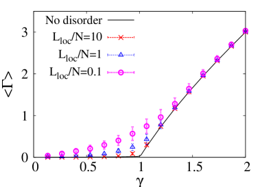
Figure 4: Mean resonance width $\langle\Gamma\rangle$ of the two superradiant states as a function of the coupling to the continuum $\gamma$ in the ballistic, chaotic, and localized regimes for disordered wires of size $N=800$. The energy $E$ was set to zero. Here, 50 wire realizations were used. The black full line corresponds to the largest eigenvalue of the non-Hermitian matrix of (5) with $\epsilon_{n}=0$.

In contrast to the mean width, the standard deviation $\sigma_{\Gamma}$ for individual widths depends strongly on the value of the localization length (see error bars in Fig. 3). Indeed, for the ballistic regime, Fig. 3(a), the region with $\gamma\sim 1$ with strong fluctuations of $\Gamma$ is quite small as compared with Fig. 3(b) and, especially, with Fig. 3(c). Thus, the fluctuations become larger as the disorder strength is increased, therefore, when the localization is stronger. Note that, independently of disorder, at the critical coupling ($\gamma=1$) the fluctuations are so strong that they are of the same size as compared to the mean value of $\Gamma$. This fact is characteristic of the phase transitions well studied in statistical mechanics.

The analysis of the error bars in Figs. 3 shows that they are independent of the system size far away from the critical coupling $\gamma=1$. This means that the product $N\sigma_{\Gamma}$ is independent of the system size in all regions. Taking into account that neither $N\langle\Gamma\rangle$ depends on the system size, one can conclude that the relative fluctuations of $\Gamma$ should not vanish in the thermodynamic limit and $\Gamma$ can not be considered as a self averaged quantity.

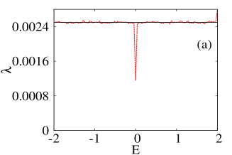
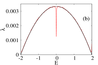
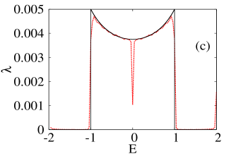
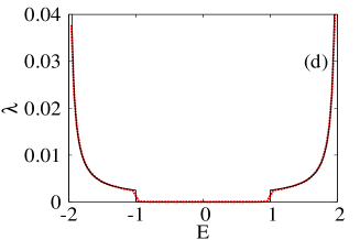
Figure 5: Inverse localization length $\lambda\equiv L^{-1}_{\mbox{\scriptsize{loc}}}$, see Eq. (15), as a function of the energy for various correlated disorders. The power spectrum $W(\mu)$ of the correlated on-site energies is given by (a) Eq. (18), (b) Eq. (20), (c) Eq. (24), and (d) Eq. (28). In all cases the disorder intensity was set to $\sigma^{2}=0.01$. Red-dashed curves correspond to numerical data (wires of length $10^{8}$ were used to compute $\lambda$), while the continuous black curves correspond to Eq. (15).

Above, we have focused our attention on the poles corresponding to long-lived states. Now, let us look at the poles that correspond to the superradiant states. In Fig. 4 we plot the mean width of the $2N_{d}$ largest-width eigenvalues, where $N_{d}$ is the number of random realizations of the non-Hermitian Hamiltonian matrix (5). For $\gamma>1$ these eigenvalues correspond to superradiant states (note that we have two leads attached to each disordered wire). In this figure we can clearly see that for large enough coupling to the continuum the mean width $\langle\Gamma\rangle$ is practically equal to the largest eigenvalue of the non-Hermitian matrix of (5) with $\epsilon_{n}=0$, see the black full line. The situation is different in the vicinity of the critical coupling $\gamma=1$, since there the disorder plays an important role. In this region it is observed that the shorter the localization length $L_{\mbox{\scriptsize{loc}}}$ the larger the mean width. A similar effect is observed for the fluctuations of the widths $\Gamma$ which acquire their largest value close to the critical coupling.

V Correlated disorder

In this Section we consider the case of weak correlated disorder, for which the Thouless expression (4) is no more valid and the corresponding localization length gets the form IKM12

$$\lambda \equiv L^{-1}_{\mbox{\scriptsize{loc}}}=\frac{\sigma^{2}}{8\sin^{2}\mu}W(\mu)\ ,$$ (15)

$$W(\mu) = 1+2\sum^{\infty}_{m=1}K(m)\cos(2\mu m)\ .$$ (16)

Here, $W(\mu)$ is the power spectrum of on-site energies $\epsilon_{n}$ and $K(m)$ is the normalized binary correlator defined as

$$K(m)=\frac{\langle\epsilon_{n}\epsilon_{n+m}\rangle}{\sigma^{2}}\ .$$ (17)

It is important to stress that Eq. (15) is valid for weak disorder, and strong deviations from this formula have been found near the band center ($\mu=\pi/2$) and the band edges ($\mu=0,\pi$), see details in Ref. IKM12 . Notice that for uncorrelated disorder we have $W(\mu)=1$ and, therefore, Eq. (15) reduces to Eq. (4). Here, $\lambda\equiv L^{-1}_{\mbox{\scriptsize{loc}}}$ is also known as the Lyapunov exponent. In what follows, we consider various types of correlations imposed to disordered potentials.

V.1 Constant localization length

In comparison with Eq. (4), expression (15) contains the additional energy-dependent term $W(\mu)$. This fact allows one to impose specific correlations for a given energy dependence of the localization length along the energy band, that is of great interest for various applications IKM12 . Let us start with the simplest, however, non-trivial case of disorder for which the localization length does not depend on energy. In this case the power spectrum takes the form,

$$W(\mu)=2\sin^{2}\mu\ ,$$ (18)

therefore, the inverse of the localization length is constant: $L^{-1}_{\mbox{\scriptsize{loc}}}=\sigma^{2}/4$. The corresponding binary correlator is given by

$$K(m)=\delta_{m,0}-\frac{1}{2}\delta_{\left|m\right|,1}\ .$$ (19)

This correlator has only three components, $K(0)=1$ and $K(\pm 1)=-1/2$, the other components vanish, thus the correlations are short-range. Figure. 5(a) shows an excellent agreement between the numerically obtained $L^{-1}_{\mbox{\scriptsize{loc}}}$ and Eq. (4), except in the vicinity of the band center where a clear resonant behavior emerges. The region near the band center has been studied in detail (see Ref. IKM12 and references therein), however in this paper we are interested in the generic properties of the localization length, therefore we focus on the energies far enough from the band center and band edges.

Correspondingly, in Fig. 6 we present the distribution of the $S$-matrix poles in the complex plane for the correlated disorder with the power spectrum of Eq. (18). The disorder increases from left to write panels; specifically, left panels correspond to weak disorder while right panels to strong disorder. The upper panels show the pole distribution for weak coupling ($\gamma\ll 1$) and the low panels are given for strong coupling ($\gamma\approx 1$).

For the ballistic regime (left panels; weak disorder) the poles are distributed around the curves corresponding to zero disorder (shown in the figure as black curves). In this regime in which all eigenstates are extended and close to plane waves, the embedded correlations in the potential do not modify strongly the distribution of poles. In contrast, in the chaotic regime (central panels) the poles are strongly scattered in the complex plane. Whereas for the localized regime (right panels), we observe the distribution of poles close to that occurring for the uncorrelated disorder. In this case, the effect of the coupling to the continuum is strongly reduced due to the small amount of eigenstates that are connected to the leads. In this case the poles are located quite close to real axis, therefore, the system should be treated as strongly isolated from the continuum. One can conclude that the most significant differences (between uncorrelated and correlated disordered wires with constant localization length) appears when the eigenstates of the Hermitian $H$ are both delocalized and chaotic. This situation occurs when the localization length is of the order of the system size (see middle panels in Fig. 6).

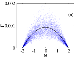
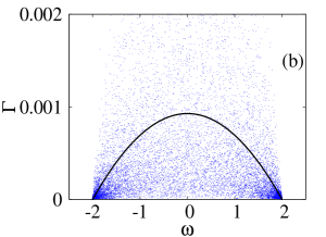
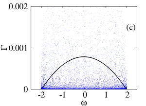
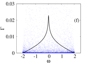
Figure 6: Imaginary vs. real part of the $S$-matrix poles $\Omega$ [see Eq. (11)] for 1D wires with correlated disorder defined by the power spectrum (18). Wires of length $N=865$ are coupled to the continuum with strengths $\gamma=0.1$ (upper panels) and $\gamma=1$ (lower panels). The disorder strength was set to $\sigma^{2}=0.001$, $L_{\mbox{\scriptsize{loc}}}/N=10$ (left panels); $\sigma^{2}=0.01$, $L_{\mbox{\scriptsize{loc}}}/N\approx 1$ (middle panels); and $\sigma^{2}=0.1$, $L_{\mbox{\scriptsize{loc}}}/N=0.1$ (right panels). Black curves represent the corresponding non-disordered wires. Here, 50 wire realizations were used.

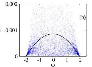
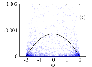
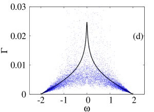
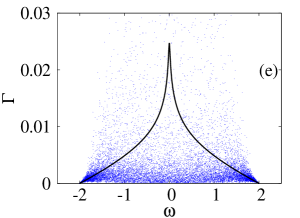
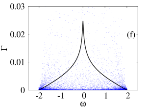
Figure 7: Imaginary vs. real part of the $S$-matrix poles $\Omega$ [see Eq. (11)] for 1D wires with correlated disorder defined by the power spectrum (20). Wires of length $N=934$ are coupled to the continuum with strengths $\gamma=0.1$ (upper panels) and $\gamma=1$ (lower panels). The disorder strength was set to $\sigma^{2}=0.001$, $L_{\mbox{\scriptsize{loc}}}/N=10$ (left panels); $\sigma^{2}=0.01$, $L_{\mbox{\scriptsize{loc}}}/N\approx 1$ (middle panels); and $\sigma^{2}=0.1$, $L_{\mbox{\scriptsize{loc}}}/N=0.1$ (right panels). Black curves represent the corresponding non-disordered wires. Here, 50 wire realizations were used.

V.2 Inverse localization length proportional to $\sin^{2}\mu$

In the uncorrelated disorder case we have $L^{-1}_{\mbox{\scriptsize{loc}}}(\mu)\propto\sin^{-2}\mu$, see Eq. (4); that is, $L^{-1}_{\mbox{\scriptsize{loc}}}$ has a minimum at $E=0$ and diverges at the energy band edges $E=\pm 2$. Using correlated disorder it is possible to invert this behavior: i.e., making $L^{-1}_{\mbox{\scriptsize{loc}}}$ to have a maximum at $E=0$ and make it vanishing at $E=\pm 2$. To this end we use the correlations defined by the power spectrum

$$W(\mu)=\frac{8}{3}\sin^{4}\mu\ ,$$ (20)

so that $L^{-1}_{\mbox{\scriptsize{loc}}}=\sigma^{2}\sin^{2}\mu/3$. Here Eq. (20) corresponds to the following binary correlator:

$$K(m)=\delta_{m,0}-\frac{2}{3}\delta_{\left|m\right|,1}+\frac{1}{6}\delta_{\left|m\right|,2}\ .$$ (21)

Thus, the non-vanishing components of $K(m)$ corresponds to $m=0$, $m=\pm 1$, and $m=\pm 2$.

The study of our model with the above correlations manifests a good correspondence between the analytical formula for the localization length (15) and numerical data as shown in Fig. 5(b). Note that a narrow resonance at the band center persists, indicating a typical deviation from Eq. (15). The corresponding pole distributions are shown in Fig. 7. One can see that the inclusion of this kind of correlated disorder does not change too much the ballistic regime picture. Indeed, the poles in Fig. 7 (left panels) are distributed pretty much the same as for the non-disordered case. As the localization length increases and reaches the chaotic regime (middle panels), the gap at the band center (clearly seen in the case of uncorrelated disorder) is now practically negligible. Finally, for the localized regime (right panels) most of the poles are located close to the real axis. A distinctive feature for this type of correlations is that most of the poles are concentrated in the vicinity of the band edges ($\omega=\pm 2$).

V.3 Mobility edges I

Now we turn our attention to an interesting situation for which the power spectrum has the form

$$W(E)=\left\{\begin{array}[]{ll}\pi/(\pi-2\mu_{1})\ ,&\quad-E_{1}<E<E_{1}\ ,\\ 0\ ,&\quad\mbox{otherwise}\ .\end{array}\right.$$ (24)

In this case the localization length in the corresponding isolated system (for $\gamma=0$) is strongly suppressed inside the energy interval $[-E_{1},E_{1}]$ and enhanced outside this interval. Thus, the critical values $\pm E_{1}$ can be treated as the mobility edges (see details and discussion in Ref. IKM12 ). Note that the value of $\mu_{1}$ is simply determined by the dispersion relation $E_{1}=2\cos\mu_{1}$. In our numerical simulation, we set $E_{1}=1$. The power spectrum (24) corresponds to the following binary correlator:

$$K(m)=\frac{1}{m(\pi-2\mu_{1})}\sin(2m\mu_{1})\ .$$ (25)

This correlator exhibits a power law decay typical of long-range correlated disorder.

The prediction of an effective delocalization transition, occurring in the first order approximation with respect to weak disorder, is corroborated in Fig. 5(c). Here, a good agreement between numerical data and the analytical expression (15) is clearly seen. A strong discrepancy emerges around the band center only, where the influence of the resonant behavior cannot be neglected.

The corresponding distributions of $S$-matrix poles are displayed in Fig. 8. In the left panels (ballistic regime) the poles whose real values belong to energy intervals where the localization length is infinite are practically equal to the corresponding poles of the non-disordered system. We term these energy intervals with $\lambda=0$ as windows of transparency, since here the transmission of waves is practically perfect. Outside of these windows, where the localization length is finite, a clear deviation from the non-disordered case is observed.

As the ratio $L_{\mbox{\scriptsize{loc}}}/N$ between the localization length and the system size decreases, the poles whose real parts belong to extended eigenstates in the windows of transparency begin to spread around the corresponding poles of the non-disorder case. The spreading of these poles is stronger as $L_{\mbox{\scriptsize{loc}}}/N$ decreases (see middle and right panels in Fig. 8). With a further decrease of $L_{\mbox{\scriptsize{loc}}}/N$, the eigenstates begin to be strongly localized and one can observe an accumulation of poles towards the real axis (see right panels of Fig. 8).

V.4 Mobility edges II

Here we show that the windows of transparency and the regions along the band with strongly localized eigenstates can be easily interchanged by the proper choice of long-range correlations. With respect to the case discussed in previous Subsection, this can be accomplished by the following power spectrum:

$$W(E)=\left\{\begin{array}[]{ll}0\ ,&\quad-E_{1}<E<E_{1}\ ,\\ \pi/2\mu_{1}\ ,&\quad\mbox{otherwise}\ .\end{array}\right.$$ (28)

With this type of correlations, the eigenstates whose eigenvalues belong to the energy interval $[E_{1},E_{1}]$ are expected to be extended, whereas the eigenvalues located outside of this energy window should correspond to localized eigenstates. This prediction is corroborated by the numerical data as Fig. 5(d) shows. Notice that now the ratio $L_{\mbox{\scriptsize{loc}}}/N$ between the localization length and the system size evaluated at the band center is infinite. Therefore, strictly speaking, the system is in the ballistic regime independently of the system size and disorder intensity. However, as we will see below, the disorder intensity still plays an important role in the distribution of poles.

The binary correlator that results in the power spectrum of Eq. (28) is given by

$$K(m)=\frac{\sin(2\mu_{1}m)}{2\mu_{1}m}\ ,$$ (29)

which exhibits a power law decay typical of long-range correlated disorder. The distributions of poles of the $S$-matrix are displayed in Fig. 9. For very weak disorder, $\sigma^{2}\lesssim 0.001$ (left panels), the poles whose real part belongs to the extended eigenstates are practically distributed as for the non-disorder case. As we increase the disorder these poles begin to spread around the corresponding poles of the non-disordered wire. In contrast, in the complementary energy windows with localized eigenstates most of the poles are located close to the real axis while the rest acquire a large imaginary part. Therefore, in these localization windows we have two effects. On the one hand the number of poles that are close to the real axis is increased as the disorder becomes stronger; on the other hand, the imaginary part of the rest of poles becomes larger (see middle and right panels of Fig. 9). If the disorder is strong enough, the distribution of poles whose real part belongs to the extended eigenstates is no longer similar to that of the poles of the non-disordered wire.

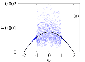
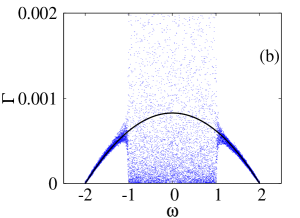
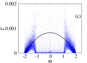
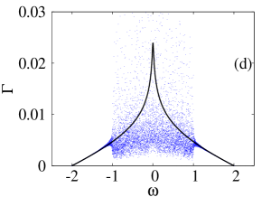
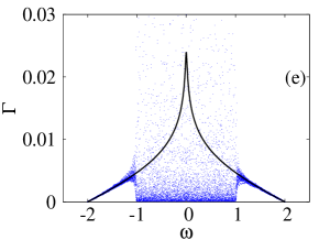
Figure 8: Imaginary vs. real part of the $S$-matrix poles $\Omega$ [see Eq. (11)] for 1D wires with correlated disorder defined by the power spectrum (24). Wires of length $N=970$ are coupled to the continuum with strengths $\gamma=0.1$ (upper panels) and $\gamma=1$ (lower panels). The disorder strength was set to $\sigma^{2}=0.001$, $L_{\mbox{\scriptsize{loc}}}/N=10$ (left panels); $\sigma^{2}=0.01$, $L_{\mbox{\scriptsize{loc}}}/N\approx 1$ (middle panels); and $\sigma^{2}=0.1$, $L_{\mbox{\scriptsize{loc}}}/N=0.1$ (right panels). Black curves represent the corresponding non-disorder wires. Here, 50 wire realizations were used.

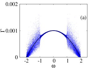
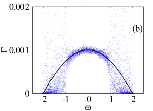
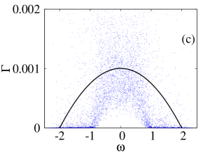
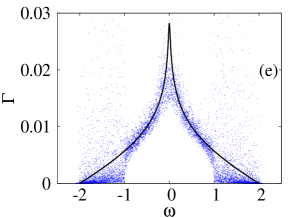
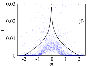
Figure 9: Imaginary vs. real part of the $S$-matrix poles $\Omega$ [see Eq. (11)] for 1D wires with correlated disorder defined by the power spectrum (28). Wires of length $N=800$ are coupled to the continuum with strengths $\gamma=0.1$ (upper panels) and $\gamma=1$ (lower panels). The disorder strength was set to $\sigma^{2}=0.001$, $L_{\mbox{\scriptsize{loc}}}/N=10$ (left panels); $\sigma^{2}=0.01$, $L_{\mbox{\scriptsize{loc}}}/N\approx 1$ (middle panels); and $\sigma^{2}=0.1$, $L_{\mbox{\scriptsize{loc}}}/N=0.1$ (right panels). Black curves represent the corresponding non-disorder wires. Here, 50 wire realizations were used.

VI Summary

We have studied 1D open tight-binding disordered wires paying main attention to the distribution of poles of the $S$-matrix in dependence on the model parameters. The model essentially depends on the system size $N$, the strength $\gamma$ of the coupling to the leads, the square-root-variance $\sigma$ of weak diagonal disorder, and on the type of disorder. In the first part of the paper we have considered uncorrelated disorder and ask the question of how the pole distribution depends on two key parameters. One of these parameters is the ratio $L_{\mbox{\scriptsize{loc}}}/N$ of the localization length $L_{\mbox{\scriptsize{loc}}}$ in the corresponding closed system (for $\gamma=0$) to the system size $N$. It is known that for perfect coupling ($\gamma=1$) this ratio determines all transport properties of the open system, a fact known as the single parameter scaling in the theory of localization, see for example Ref. M99 . According to this parameter, we consider three characteristic situations: extended eigenstates with $L_{\mbox{\scriptsize{loc}}}\gg N$ (plane waves slightly modified by disorder), extended chaotic eigenstates with $L_{\mbox{\scriptsize{loc}}}\sim N$, and localized eigenstates with $L_{\mbox{\scriptsize{loc}}}\ll N$.

The analysis of the pole distribution in dependence on $L_{\mbox{\scriptsize{loc}}}/N$ and $\gamma$ has shown that for the effectively weak disorder ($L_{\mbox{\scriptsize{loc}}}\gg N$) the location of poles in the complex plane follows those occurring for a non-disordered potential ($\sigma=0$ and $\gamma=0$). In the other limit case of relatively strong disorder ($L_{\mbox{\scriptsize{loc}}}\ll N$) it was found that the pole distribution is very different from the previous case. Specifically, the data clearly demonstrates that, when in the closed wire the eigenstates are strongly localized, in the open wire the poles are mainly located close to the real axis. With the increase of coupling to the leads this effect is enhanced. It is important to stress that even for weak disorder, the effect of attraction of the poles to the real axis cannot be neglected (see the data in Figs. 1 and 2).

Another question is how the mean value of the imaginary parts of the poles depends on the strength of the coupling to the leads. Note that the poles of the $S-$matrix give the information about the widths of the resonances appearing in the transmission of waves through finite disordered wires. These resonances can easily be observed experimentally, at least for the poles with a small imaginary part. Our key idea was that the dependence of the mean value of the imaginary parts of the poles on the coupling strength is similar to that described by the famous Moldauer-Simonius relation (13). Although this relation has been derived for random matrix models, one can expect that Eq. (13) is also valid for low-dimensional models such as the model studied here. The numerical data reported in Fig. 3 clearly support our expectation. Thus our results indicate that the area of application of the Moldauer-Simonius relation (13) is much broader than it was initially expected.

The most important feature described by the Moladauer-Simonious relation is that at the critical point, $\gamma=1$, the mean value of the widths $\Gamma$ diverges. This remarkable fact is well seen in Fig. 3, also demonstrating an increase of fluctuations of individual $\Gamma$ at the critical point. Note that these two effects seem to be independent of the degree of localization, $L_{\mbox{\scriptsize{loc}}}/N$. However, the fluctuations themselves are increased with the decrease of this ratio, therefore, with the increase of the disorder. It should be stressed that the divergence of the mean of widths at $\gamma=1$ can be treated as an indication of a phase transition, for which the fluctuations are of the order of the mean values. This effect is known as the superradiance transition well studied in terms of full random matrices in place of the real part $H$ in non-Hermitian Hamiltonians brody81 .

In order to better present the data characterizing the superradiant transition, we have plotted the mean values of $\Gamma$ for two poles (for each wire) with the largest values of $\Gamma$. In the region $\gamma<1$ there is only one cloud of poles in the complex plane and all the poles have effectively small imaginary parts (the region of isolated resonances). When the coupling exceeds the critical value $\gamma=1$, two of the $N$ poles have very large values of their imaginary parts in comparison with all other poles that move back to the real axis with the increase of the coupling. This effect is clearly seen in Fig. 4, where the mean value of the largest $\Gamma$ is plotted. As one can see, for $\gamma<1$ the influence of localization is strong for localized states, however, for $\gamma>1$ the effect of the localization is negligible.

In the second part of the paper we addressed the question of the influence of correlations, imposed to the diagonal disorder, on the pole distribution. We have considered few types of disorder with either short-range or long-range correlations. Having in mind the analytical results obtained for all these cases in the weak disorder limit, first in Fig. 5 we plotted the localization length versus energy for the potentials with correlations, in comparison with the analytical predictions. Our data demonstrate that the method, used for the creation of random disorder resulting in specific dependences of the localization length on energy, works perfectly in the presence of coupling to continuum.

With the use of the theory of correlated disorder one can create the energy windows where the localization length is much larger that the length $N$ of the wires, together with the windows where the eigenstates are strongly localized. In this way, one can speak of effective band edges. The data in Fig. 5 demonstrate an excellent agreement between the numerically found localization length and the analytical predictions. However, a quite strong discrepancy occurs for energies close to the band center; an effect which is well studied in the literature (see for example the review in Ref. IKM12 ). The origin of this discrepancy is the failure of the standard perturbation theory used to derive the analytical expression for the localization length.

With the reference to Fig. 5, where the localization length is plotted versus energy, we have analyzed the distribution of poles when correlations are imposed into disorder in the presence of coupling to the leads. In Figs. 6 and 7 the pole distribution is shown for correlated disorder without mobility edges in dependence on the disorder strength and on the degree of the coupling. The analysis shows that, in general, with the increase of disorder the poles begin to be more scattered in comparison to the non-disordered wires. Another conclusion is that for both weak and strong disorder the poles tend to be concentrated near the real axis. As for the correlated disorder resulting in the mobility edges, see Figs. 8 and 9, the most important conclusion is that in the presence of coupling to the leads the distribution of the poles of the scattering matrix mainly follows that occurring in the absence of disorder, provided the coupling parameter $\gamma$ is not too large. On the other hand, strong coupling to the continuum essentially modifies the distribution of poles, however, mainly in those energy windows where the eigenstates are strongly localized.

VII acknowledgments

We acknowledge G. L. Celardo for pointing out relevant references to us. F.M.I. acknowledges support from VIEP-BUAP (Grant No. IZF-EXC13-G). J.A.M.-B. acknowledges support from VIEP-BUAP (Grant No. MEBJ-EXC18-G), Fondo Institucional PIFCA (Grant No. BUAP-CA-169), and CONACyT (Grant No. CB-2013/220624).

References

- (1) F. M. Izrailev, A. A. Krokhin, and N. M. Makarov, Phys. Rep. 512, 125 (2012).
- (2) I. M. Lifshits, S. A. Gredeskul, and L. A. Pastur, Introduction to the Theory of Disordered Systems (Wiley, New York, 1988).
- (3) N. M. Makarov, Spectral and Transport Properties of One-Dimensional Disordered Conductors (Lecture Notes, 1999). http://www.ifuap.buap.mx/virtualrev/ documentos/lecnot-r.pdf
- (4) C. Mahaux and H. A. Weidenmüller, Shell Model Approach to Nuclear Reactions, (North Holland, Amsterdam, 1969).
- (5) J. J. M. Verbaarschot, H. A. Weidenmüller, and M. R. Zirnbauer, Phys. Rep. 129, 367 (1985).
- (6) V. V. Sokolov and V. G. Zelevinsky, Phys. Lett. B 202, 10 (1988); Nucl. Phys. A504, 562 (1989); I. Rotter, Rep. Prog. Phys. 54, 635 (1991); Ann. Phys. (N.Y.) 216, 323 (1992); F. Haake, F. M. Izrailev, N. Lehmann, D. Saher, H.-J. Sommers, Z. Phys. B 88, 359 (1992).
- (7) D. J. Thouless, in Ill-condensed matter, eds. R. Balian, R. Maynard and G. Toulouse (Amsterdam: North-Holland, 1979).
- (8) S. Sorathia, F. M. Izrailev, V. G. Zelevinsky, and G. L. Celardo, Phys. Rev. E 86, 011142 (2012).
- (9) T. A. Brody, J. Flores, J. B. French, P. A. Mello, A. Pandey, and S. S. M. Wong, Rev. Mod. Phys. 53, 385 (1981).
- (10) J. B. French and S. S. M. Wong, Phys. Lett. B 33, 449 (1970) ; J. French, S. Wong, Phys. Lett. B 35, 5 (1971) ; O. Bohigas, J. Flores, Phys. Lett. B 34, 261 (1971); O. Bohigas and J. Flores, Phys. Lett. B 35, 383 (1971) ; K. Mon and J. French, Ann. Phys. 95, 90 (1975) .
- (11) A. Volya and V. Zelevinsky, AIP Conf. Proc. 777, 229 (2005).
- (12) G. L. Celardo and L. Kaplan, Phys. Rev. B 79, 155108 (2009); G. L. Celardo, A. M. Smith, S. Sorathia, V.G. Zelevinsky, R.A. Sen’kov, and L. Kaplan, Phys. Rev. B 82, 165437 (2010).
- (13) G. L. Celardo, A. Biella, L. Kaplan, and F. Borgonovi, Fortschr. Phys. 61, 250 (2013).
- (14) M. Weiss, J. A. Mendez-Bermudez, and T. Kottos, Phys. Rev. B 73, 045103 (2006).
- (15) G. L. Celardo, F. M. Izrailev, V. G. Zelevinsky, and G. P. Berman, Phys. Lett. B 659, 170 (2008).
- (16) Y. V. Fyodorov and H.-J. Sommers, JETP Lett. 63, 1026 (1996).
- (17) P. A. Moldauer, Phys. Rev. 157, 907 (1967); M. Simonius, Phys. Lett. B 52, 279 (1974); Y. V. Fyodorov and H.-J. Sommers, J. Math. Phys. 38, 1918 (1997); H.-J. Sommers, Y. V. Fyodorov, and M. Titov, J. Phys. A 32, L77 (1999); G. L. Celardo, F. M. Izrailev, V. G. Zelevinsky, and G. P. Berman, Phys. Rev. E 76, 031119 (2007).
- (18) Y. V. Fyodorov, in 2016 URSI International Symposium on Electromagnetic Theory (EMTS), Espoo, Finland, 2016, pp. 666-669.