Characterizing the Nature of the Yielding Transition

Abstract

Particulate matter, such as foams, emulsions, and granular materials, attain rigidity in a dense regime: the rigid phase can yield when a threshold force is applied. The rigidity transition in particulate matter exhibits bona fide scaling behavior near the transition point. However, a precise determination of exponents describing the rigidity transition has raised much controversy. Here, we pinpoint the causes of the controversies. We then establish a conceptual framework to quantify the critical nature of the yielding transition. Our results demonstrate that there is a spectrum of possible values for the critical exponents for which, without a robust framework, one cannot distinguish the genuine values of the exponents. Our approach is two-fold: (i) a precise determination of the transition density using rheological measurements and (ii) a matching rule that selects the critical exponents and rules out all other possibilities from the spectrum. This enables us to determine exponents with unprecedented accuracy and resolve the long-standing controversy over exponents of jamming. The generality of the approach paves the way to quantify the critical nature of many other types of rheological phase transitions such as those in oscillatory shearing.

I Introduction

Yield stress materials such as toothpaste, hair gel, mayonnaise, and cement, are ubiquitous. These materials are used in pharmaceutical and cosmetics manufacturing, as well as the oil, concrete, and food industries Bonn et al. (2017). Because of their wide applicability in everyday life, a quantitative description of their rheological behavior is pivotal. The physical origin of the yield stress depends on the microscopic details of the system and can be classified into three main categories: dynamic arrest in Brownian suspensions known as the glass transition Petekidis et al. (2004), mechanical (meta)stability in athermal systems or jamming Liu and Nagel (1998); Paredes et al. (2013), and attractive interactions Trappe et al. (2001); Rahbari et al. (2013). Thixotropic yield stress fluids Bonn et al. (2017), which exhibit memory effects and a bifurcation in the viscosity, are outside the focus of the current study.

The relation between shear stress $\sigma$ and shear rate $\dot{\gamma}$, known as a flow curve in a yield stress material, can be described as a Herschel-Bulkley (HB) relation:

$$\sigma=\sigma_{y}+K\dot{\gamma}^{\Delta},$$ (1)

where $\sigma_{y}$ is the yield-stress and $\Delta<1$ is the shear thinning exponent. In contrast, a simple Newtonian fluid is described by a single parameter, namely the shear viscosity $\eta=\sigma/\dot{\gamma}$. As a result of the threshold $\sigma_{y}$, the viscosity of a yield stress material diverges for $\dot{\gamma}\to 0$. However, Barnes and Walters Barnes and Walters (1985) demonstrated that carbopol microgels have finite viscosity at small shear rates and raised a historical debate over the existence of the yield stress. Two decades later, Möller et al.  Moeller et al. (2009) repeated the same experiment and showed that those measurements at low shear stresses never reached a stationary state and that the apparent finite viscosity was an artifact of the measurement.

A consensus regarding the existence of the yield stress has emerged. However, the technical difficulties of its measurements remain a challenge. Despite these advances in the understanding of the yield stress, a description of the non-linear flow curves in the fluid state remains an open problem. In the traditional approach, the shear-thinning exponent $\Delta$ is obtained by a power law fit to $\sigma-\sigma_{y}$ versus $\dot{\gamma}$. However, recent numerical simulations showed that $\sigma-\sigma_{y}$ vs $\dot{\gamma}$ exhibits two distinct scaling regimes described by two different exponents, $\Delta$ and $\Delta^{\prime}$, for small and large shear rates Olsson and Teitel (2011); Lerner et al. (2012); Kawasaki et al. (2015), respectively. As a result, fitting a HB-type relation to such data will be prone to pitfalls due to a bias towards larger shear rates, which in turn will give rise to a misleading quantification of the flow curves.

The problem becomes even more dramatic for the case of matter with granularity Schall and van Hecke (2010). Soft particulate matter, such as gels and emulsions, flow freely in the dilute regime and attain yield stress above a threshold density $\phi_{J}$ in the dense regime. This yielding transition exhibits a rich class of scaling behavior of the flow curves described by critical exponents (we will give a brief overview about different scaling regimes of the rigidity transition in the next section). Despite many efforts by different groups Hatano (2008); Otsuki and Hayakawa (2009a); Hatano (2010); Otsuki and Hayakawa (2012); DeGiuli et al. (2015); Vagberg et al. (2016), a precise determination of the critical exponents remains disputed.

Here, we establish a conceptual framework for the scaling quantification of the flow curves of a wide range of yield stress materials. We resolve the long-standing dispute over exponents of the rigidity transition.

II Rigidity transition: a bird’s eye view

Depending on the shear rate and packing fraction, soft frictionless spheres display a rich phenomenology of distinct rheological regimes. This makes soft frictionless spheres Drosophila of particulate matter.

In the dilute regime of particulate materials, flow curves at small shear rates are given by $\sigma\propto\dot{\gamma}^{n}$ where $n=1$ and $2$ for Newtonian and Bagnoldian scalings, respectively. Because soft particles barely deform at small shear rates, $\sigma\propto\dot{\gamma}^{n}$ corresponds to the so-called hard-core limit. The exponent $n$ has been shown to depend on the Reynolds number of the system such that for overdamped systems the Newtonian regime (non-inertial) is recovered and for $n=2$ the system must be under-damped (inertial) Vagberg et al. (2014a). The transport coefficient, which is given by shear viscosity $\eta=\sigma/\dot{\gamma}^{n}$, at $\dot{\gamma}\to 0$, depends only on the packing fraction $\phi$ and diverges upon approaching the jamming density $\eta\propto|\delta\phi|^{-\beta}$, where $\delta\phi=\phi-\phi_{J}$ is the distance from jamming. The exponent $\beta$ also characterizes the hard-core limit of the system. Accordingly, this exponent must be independent from the microscopic details of the system Olsson and Teitel (2012); Vagberg et al. (2014b). At $\phi=\phi_{J}$, the system exhibits pure power-law rheology $\sigma\propto\dot{\gamma}^{q}$ with $q<1$ as the critical shear-thinning exponent. In the soft core regime $\phi>\phi_{J}$, the system displays threshold rheology and flow curves that may be described by the HB model given by Eq. 1. In this model, the shear-thinning exponent $\Delta$ is shown to be related to the behavior of the system in the hard-core limit at $\phi<\phi_{J}$ and thus to the exponent $\beta$ Olsson and Teitel (2012). The yield stress also scales with the distance from jamming $\sigma_{y}\propto\delta\phi^{y}$.

As one can see, upon approaching the jamming point, the rheology changes dramatically due to the collective behavior of particles Radjai and Rou (2002). Consequently, the rheology can no longer be described by trivial exponents such as $n=1$ or $2$ and thus the system becomes shear-thinning with a non-trivial scaling dimension $q<1$. This is a signature of a growing length scale in the system  Olsson and Teitel (2011); Olsson (2015); Nordstrom et al. (2010), which is the hallmark of critical phenomena. Even though this system is non-equilibrium and athermal, Olsson and Teitel Olsson and Teitel (2007) used renormalization group formalism Kardar (2007) of equilibrium phase transitions to capture the critical nature of this dynamic transition. The jamming point at $\delta\phi=0,\dot{\gamma}\to 0,T=0,$ and $L\to\infty$ is a genuine dynamic critical point.

Altogether, any of the above scaling limits can be retrieved by choosing appropriate limits of a scaling function $\mathcal{F}_{0}$ and an arbitrary length scale $b$ in the following scaling ansatz: (derivation given in Appendix B):

$$\sigma(\delta\phi,\dot{\gamma},L,w)=b^{-y/\nu}\;\mathcal{F}_{0}(\delta\phi\>b^{1/\nu},\dot{\gamma}\>b^{z},L^{-1}\>b,w\>b^{-\omega}),$$ (2)

where $\mathcal{F}_{0}$ is a homogeneous scaling function, $L$ is the system size, and $w$ is an auxiliary variable. This scaling ansatz is traditionally used to find relations between different exponents. Inserting $b=\dot{\gamma}^{-1/z}$ for $L\to\infty$ in Eq. 2, we arrive at:

$$\sigma=\dot{\gamma}^{q}\mathcal{F}_{1}\left(\frac{\delta\phi}{\dot{\gamma}^{q/y}}\right),$$ (3)

where $q=y/(z\nu)$. Here, we assume proximity of the critical point where the auxiliary variable $w$ can be neglected.

The immediate outcome of Eq. 3 is that all the data must collapse into a master curve when plotted $\sigma/\dot{\gamma}^{q}$ vs ${\delta\phi}/{\dot{\gamma}^{q/y}}$, providing that three free parameters $q$, $y$, and $\phi_{J}$, are fine tuned. Notably, in the early stage of this topic, this method, ı.e., collapse of the data, has been extensively used by many authors to estimate $q$, $y$, and $\phi_{J}$ Olsson and Teitel (2007); Hatano (2008, 2010); Otsuki and Hayakawa (2012); Hayakawa and Otsuki (2013). A summary of the existing predictions for these exponents is given in Tab. 1. These reports were not conclusive because of the large range of reported exponents and critical densities. The reason for this was because the quality of the collapses were judged based on the visual appeal of the plots. Later, Olsson and Teitel used a quantitative method to compute the quality of the collapses. The method was based on (i) exponential parametrization of the scaling function $\mathcal{F}_{1}(x)=\exp\left(\sum_{n=0}^{5}a_{n}x^{n}\right)$ and (ii) going into unprecedented small shear rates down to $10^{-8}$ in the dimensionless scale Olsson and Teitel (2011); Vagberg et al. (2016). However, the expansion of $\mathcal{F}_{1}(x)$ may be prevented because, as $x\to 0$, $\mathcal{F}_{1}(x)$ may not be analytic. Also, for reasons that we describe in the next paragraph, going into shear rates as small as $\dot{\gamma}\approx 10^{-8}$ contaminates the scaling behavior.

$$\begin{array}[]{llll}\hline\cr\hline\cr\text{authors}&y&q&\omega/z\\ \hline\cr\\[-5.69054pt] \text{Otsuki \& Hayakawa (theory)~{}\cite[cite]{\@@bibref{Authors Phrase1YearPhrase2}{otsuki_2009_2}{\@@citephrase{(}}{\@@citephrase{)}}}}&1&2/5&-\\[2.84526pt] \text{Hatano~{}\cite[cite]{\@@bibref{Authors Phrase1YearPhrase2}{hatano_2008}{\@@citephrase{(}}{\@@citephrase{)}}}}&1.2&0.63&-\\[2.84526pt] \text{Hatano~{}\cite[cite]{\@@bibref{Authors Phrase1YearPhrase2}{hatano_2010}{\@@citephrase{(}}{\@@citephrase{)}}}}&1.5&0.6&-\\[2.84526pt] \text{Otsuki \& Hayakawa (simul.)~{}\cite[cite]{\@@bibref{Authors Phrase1YearPhrase2}{otsuki_2012}{\@@citephrase{(}}{\@@citephrase{)}}}}&1.09&0.46&-\\[2.84526pt] \text{DeGiuli~{}{ \it et al.~{}}~{}\cite[cite]{\@@bibref{Authors Phrase1YearPhrase2}{degiuli_2015}{\@@citephrase{(}}{\@@citephrase{)}}}}&1&0.3&0.3\\[2.84526pt] \text{Vagberg~{}{ \it et al.~{}}~{}\cite[cite]{\@@bibref{Authors Phrase1YearPhrase2}{vagberg_2016}{\@@citephrase{(}}{\@@citephrase{)}}}}&1.15(5)&0.38(5)&0.35(7)\\[2.84526pt] \text{Goodrich{ \it et al.~{}}~{}\cite[cite]{\@@bibref{Authors Phrase1YearPhrase2}{goodrich_2016}{\@@citephrase{(}}{\@@citephrase{)}}}}&1&-&-\\ \hline\cr\hline\cr\end{array}$$

Table 1: Critical exponents reported by different authors. As the data get closer to the critical point, exponents systematically change (for a comprehensive discussion, cf.  Vagberg et al. (2016)).

It is well known that in the jammed state a sheared particulate system exhibits shear localizations, also known as shear-transformation-zones Maloney and Lemaître (2006); Bouchbinder et al. (2007). These stress anomalies relax through long-range system-wide avalanches. Each avalanche can trigger other active zones that will in turn result in a domino of plastic events and relaxations. At very small shear rates, these avalanches are globally correlated and poise the system into an effective critical state Lemaitre and Caroli (2009); Hentschel et al. (2010). This results in scale-free distributions of avalanches with exponents that are generally smaller than 2 Hatano et al. (2015); Nicolas et al. (2017). To obtain a flow curve $\sigma\left(\dot{\gamma}\right)$, one should perform time averaging for shear stress over the time series. However, due to the scale-free distribution of avalanches with the aforementioned range of exponents, the first and second moments of the shear stress cannot be well-defined. Consequently, the time averaged shear stress at very small shear rates possesses error bars that are as large as the average values.

To avoid the above problems, we describe a general framework that requires neither data collapse nor expansion of the scaling function. Additionally, measurements are performed outside the avalanche region, ı.e., not at very small shear rates. These simplify the problem dramatically and enable us to resolve the controversy over exponents. Our approach is two-fold: first, in Sec. III, we describe how we nail down the critical density. Second, in Sec. IV, we present our matching rule that selects critical exponents from a wide spectrum of possible values.

III Hunt for $\phi_{J}$

Precise determination of the critical exponents strongly depends on whether the critical density $\phi_{J}$ is accurately determined. In this section, we explain how we nail down the transition density $\phi_{J}$ using rheological data. To achieve this goal, we define successive slopes of the flow curves $m$ as:

$$m=\frac{d\ln\sigma}{d\ln\dot{\gamma}},$$ (4)

where $d$ stands for the derivative. This can be easily calculated from Eq. 3:

$$m=q-\frac{q}{y}\frac{\delta\phi}{\dot{\gamma}^{q/y}}\frac{\mathcal{F}_{1}^{\prime}(x)}{\mathcal{F}_{1}(x)},$$ (5)

where $x={\delta\phi}/{\dot{\gamma}^{q/y}}$, $\mathcal{F}_{1}^{\prime}(x)=d\mathcal{F}_{1}(x)/dx$.

Eq. 5 provides an immediate prediction: if one plots $m$ vs $\dot{\gamma}$ for different packing fractions, exactly at jamming density $\delta\phi=0$, the successive slope for all shear rates will be equal to the critical shear-thinning exponent $m=q$. For $\delta\phi>0$, the successive slope converges to $m=q$ at large shear rates and deviates from that value for $\dot{\gamma}\to 0$ according to $\dot{\gamma}^{-q/y}$. Similar behavior is expected for $\delta\phi<0$ with an opposite curvature.

This provides a simple recipe to compute $\phi_{J}$: the critical density is given by a horizontal line of the $m-\dot{\gamma}$ dependence that distinguishes off-critical densities with opposite curvatures. However, it is practically impossible to recover a straight horizontal line for $m$ at $\phi_{J}$ in the critical region of $\dot{\gamma}\to 0$. This is due to elasto-plastic critical fluctuations near the critical point, which we mentioned in Sec. II.

The remedy for this problem is to stay away from the region where the successive slope displays huge fluctuations. In such a regime, correction-to-scaling must be taken into account. From Eq. 2, the leading correction-to-scaling term at $\phi=\phi_{J}$ reads:

$$\sigma=\dot{\gamma}^{q}\left(c_{1}+c_{2}\dot{\gamma}^{\omega/z}\right),$$ (6)

where $c_{1}$ and $c_{2}$ are constants and $\omega/z$ is the leading correction-to-scaling exponent (see Appendix B for derivation). For off-critical densities $\phi\neq\phi_{J}$, an extra term proportional to $\delta\phi$ must be added to Eq. 6. This term again has an inverse algebraic dependence on $\dot{\gamma}$ similar to that in Eq. 5. One can easily calculate the corresponding successive slope of Eq. 6 as:

$$m=q+k\dot{\gamma}^{\omega/z},$$ (7)

where $q$ is the asymptotic exponent and $k$ is a constant. This shows the behavior of the successive slopes at $\phi_{J}$, which distinguishes that of off-critical densities with opposite curvatures.

Now let us calculate the asymptotic values of the successive slopes for different densities at $\dot{\gamma}\to 0$. For $\delta\phi<0$, $\sigma\propto\dot{\gamma}^{n}$, which results in $m=n$. At $\delta\phi=0$, $\sigma\propto\dot{\gamma}^{q}$, then $m=q$. For $\delta\phi>0$, the yield stress emerges, which amounts to a dependence $\propto\dot{\gamma}^{0}$ and thus $m=0$. In summary:

$$\lim_{\dot{\gamma}\to 0}m=\left\{\begin{array}[]{lr}n&\phi<\phi_{J}\\ q&\phi=\phi_{J}\\ 0&\phi>\phi_{J}.\\ \end{array}\right.$$ (8)

We summarize the behavior of the successive slope of flow curves in a schematic diagram in Fig. 1. This diagram demonstrates the simplicity behind our framework to find $\phi_{J}$. In a semi-log plot of $m$ vs $\dot{\gamma}$, all of the sub- and super-critical densities curve in opposite directions, except at $\phi_{J}$.

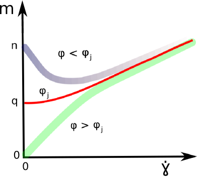
Figure 1: Schematics of successive slope. A schematic figure shows the successive slope vs shear rate in a semi-log scale. According to Eq. 5, curves at sub- and super-critical densities have opposite curvatures. In the asymptotic limit $\dot{\gamma}\to 0$, all curves converge to the asymptotic exponents given by Eq. 8. The curve corresponding to $\phi_{J}$ is the only curve that does not bend upward or downward and whose offset is equal to the non-trivial critical exponent $q$.

In our strategy to find $\phi_{J}$, we first obtain flow curves for an intermediate system size. We mark the range of densities where the curvature of the successive slopes changes. We then zoom into the region by simulating a larger system size and nail down $\phi_{J}$. Finally, we check whether our estimated $\phi_{J}$ is robust against finite-size effects.

We perform extensive large-scale two dimensional molecular dynamics simulations of frictionless disks in a simple shear flow. In our simulations, we dissipate the normal component of the relative velocity of colliding particles. This dissipation law leads to Bagnoldian scaling in the dilute regime. The Newtonian regime is recovered when the transverse component of the relative velocity is dissipated Vagberg et al. (2014b). This regime is not explored in this work. Further details of the simulations are given in Appendix A. In Fig. 2, we display the successive slope $m$ vs shear rate $\dot{\gamma}$ for different packing fractions $\phi$ for a system of intermediate size $L=100$. The curvature of the curves changes in the range between $\phi=0.843$ and $0.844$. This determines the window for $\phi_{J}$. We will zoom into this region to determine $\phi_{J}$ with a higher resolution and larger system sizes. All of the curves corresponding to different packing fractions show a tendency to converge at large shear rates. This is in accord with the predictions by Eq. 5. One can see that upon decreasing the shear rate, the far-top curves show a tendency to converge towards the value of the asymptotic exponent $n=2$ and the far-bottom curves to $0$. This is again in accord with the prediction by Eq. 8. A dashed line shows an estimation for the value of $q=0.6$. We note that this line tends towards smaller values upon increasing $L$. For $L\geq 200$, the estimated value of $q$ does not change. We note that for $\dot{\gamma}<10^{-6}$, the successive slope in the critical range of densities displays giant fluctuations reminiscent of critical fluctuations. We observe these fluctuations for systems of larger spatial extents for $\dot{\gamma}<10^{-6}$. Therefore, in the rest of the paper, we do not consider data with $\dot{\gamma}<10^{-6}$ in our analysis. To summarize the results for $L=100$, the crude estimation for the transition density is $\phi_{J}\approx 0.84335\pm 0.00035$. The naïve estimation for the critical exponent is $q\approx 0.6$. Next, we will zoom into the critical region with substantially larger system sizes to find $\phi_{J}$.

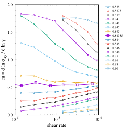
Figure 2: Successive slope. Successive slope $m$ vs shear rate $\dot{\gamma}$ for different $\phi$. The value of each $\phi$ is given in the legend. The number of particles varies from $N=7183$ to $7742$ for $\phi=0.835$ and $0.90$, respectively. The spatial extent of the system is $L=100$. The curvature of the curves changes in the range of $\phi=0.843$ and $0.844$. This marks the critical window for $\phi_{J}$ and the range for refined measurements with a much larger resolution on $\phi$ for substantially larger system sizes.

According to elasticity theory, shear stress and pressure are both components of a single entity known as the stress tensor. Different components of the stress tensor provide information about momentum transfer in different directions into/along imaginary surfaces in the system Landau and Lifshitz (1986). However, whether the shear stress and pressure scale equivalently with shear rate is not at all an obvious fact. According to Peynneau and Roux Peyneau and Roux (2008) and more recently by Baity et al.  Baity-Jesi et al. (2017) a finite stress anisotropy, $\delta p\propto p_{xx}-p_{yy}$, gives rise to a small rotation of principal axes of of the stress tensor from those given by the strain tensor. This gives rise to distinct scaling of the shear stress and pressure when there is a stress anisotropy in the system; this usually happens at high shear rates. However, the stress anisotropy is negligible at small shear rates near jamming Vagberg et al. (2017). This is also confirmed by our results. Thus, it is a widely accepted fact that the asymptotic scaling of the shear stress and pressure are equivalent. This assumption has been adopted by many recent studies, cf.  Vagberg et al. (2016). More recently, Suzuki and Hayakawa provided a rigorous derivation of this based on a $\mu$-$J$ rheology Suzuki and Hayakawa (2017). We will use this assumption in the next section to nail down the critical exponent $q$.

We display refined measurements in Fig. 3 for different system sizes up to $L=300$. Panel a and b refer to the successive slopes of the shear stress and pressure, respectively. One can see that for all densities, there is a strong system size dependence for $L<200$. For $L\geq 200$, the successive slopes are on top of each other for all densities. The curves at $\phi=0.843$ and $0.844$ clearly have opposite curvatures for all system sizes. We zoom into this region to find the critical density. Filled squares correspond to $\phi=0.84335$ and $L=300$. These data are averaged over $7$ different ensembles. The rest of the data are obtained from a single realization. For $L=300$, a closer inspection of data at $\phi=0.8433$ and $0.8434$ reveals their opposite curvatures. The $\phi=0.84345$ line is curved down similar to that at $\phi=0.8434$. Therefore, these are off-critical densities. However, one can clearly see that $\phi=0.84335$ (filled squares) is the cross-over density where the curvature changes. Therefore, we conclude $\phi_{J}=0.84335\pm 0.00005$. Interestingly, our estimated density within error bars agrees with that of Heussinger et al.  Heussinger and Barrat (2009) and Vagberg et al.  Vagberg et al. (2016). A closer inspection of the successive slope of shear stress $\sigma$ (panel a) and pressure $p$ (panel b) reveals a stronger corrections-to-scaling of the shear stress. Here, stronger corrections-to-scaling means a larger amplitude of the scaling function of Eq. 7. However, as we have mentioned in the previous paragraph the asymptotic exponents must be equivalent for both pressure and shear stress. Interestingly, a stronger corrections-to-scaling of shear stress has been reported by other authors  Olsson and Teitel (2011); Vagberg et al. (2016).

One can see that $\phi_{J}$ does not have a strong dependence on the system size. However, the asymptotic exponent changes continuously from $0.6$ to approximately $0.4$ by increasing the system size from $L=50$ to $300$, respectively. Estimation of $q$ for $L=300$ is not straightforward because of the complexity of the scaling function for large system sizes, ı.e., the dependence of $m$ to $\dot{\gamma}$. In the next section, we describe a systematic method to nail down the critical exponents.

      

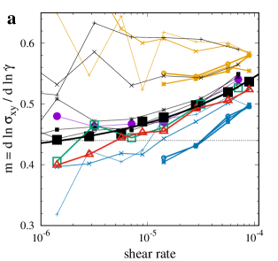
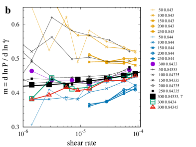
Figure 3: Successive slope of refined measurements. Successive slope versus shear rate for (a) shear stress and (b) pressure. The critical density is found $\phi_{J}=0.84335$. We observe a strong system size dependence for $L\leq 200$. For $L\geq 250$, different system sizes are on top of each other. In this density, for $L=300$, the system consists of $N=65397$ particles. The successive slopes at slightly above and below $\phi_{J}$ bend in opposite directions. A stronger correction-to-scaling is found for the shear stress $\sigma$.

IV Hunt for exponents

In this section, we describe how we nail down the critical exponents. The easiest way to find critical exponents is to obtain them via fitting Eq. 7 to the successive slope curve at $\phi_{J}$ in Fig. 3 using $q$, $k$, and $\omega/z$ as free fitting parameters. We call this a blind fitting. Notably, a $3$-parameter fitting corresponds to the optimization of a residual function in a $3+1$ dimensional space. This function is rugged and has many local basins. Each fitting algorithm/software will find one such local minimum. This will cause a zoo of different values for the exponents due to the rugged nature of the residual function.

To avoid fitting artifacts, we hold the correction-to-scaling exponent $\omega/z$ fixed and obtain the asymptotic exponent $q$ via fitting a linear function to $m$ versus $\dot{\gamma}^{\omega/z}$. We vary $\omega/z$ in a range between $0.3$ and $0.5$, and we record the corresponding $q$. The contour lines of the fits are given in Fig 4-a for both shear stress and pressure. Each contour line represents all possible outcomes of $q$ and $\omega/z$ via a $3$-parameter blind fitting. Each point on the contour lines corresponds to one basin. Now, the crucial question becomes about which point on the contour line can be considered the corresponding point for correct exponents.

As we previously noted, pressure and shear stress can have different scaling functions; however, asymptotic critical exponents must strictly be equivalent. This provides a matching rule, which allows us to pick up the correct exponents based on the crossing point of the contour lines of $p$ and $\sigma$. Fig. 4-a demonstrates that such a matching point really does exist, and we read exponents $q=0.41$ and $\omega/z=0.365$ for both $p$ and $\sigma$. We note that within error bars, the crossing point gives the same $q$ for $L\geq 200$. However, $\omega/z$ is not stable. Therefore, we perform the finite-size scaling analysis for $\omega/z$ with fixed $q\left(L=\infty\right)=0.41$ via

$$m\left(L\right)-q\left(L=\infty\right)\propto\dot{\gamma}^{\omega/z\left(L\right)}.$$ (9)

We fit Eq. 9 and obtain $\omega/z$ as a function of $L$. We plot $\omega/z\left(L\right)$ vs $L^{-1}$ in Fig. 4-b. One can see that $\omega/z$ levels off at $0.35$ for the largest system sizes. This gives us the asymptotic value of the leading correction-to-scaling exponent $\omega/z\left(L=\infty\right)=0.35$. We summarized the values of critical exponents in Tab. 2.

Having obtained both $q\left(L=\infty\right)$ and $\omega/z\left(L=\infty\right)$, we arrive at our final vital benchmark. We now hold $q$ and $\omega/z$ fixed to their asymptotic $L=\infty$ values and fit Eq. 7 to the data to obtain the amplitude $k$. The resulting curves are shown as solid lines in both Fig. 3-a and -b. We obtain $k=3.7$ and $1.36$ for shear stress and pressure, respectively. Since $k$ is the amplitude of the leading correction-to-scaling term, which is supposed to be a small term, $k$ must be $\mathcal{O}(1)$. This dramatically depends on the window of $\dot{\gamma}$. If this window is far from the critical region, then the next terms in the correction-to-scaling must be considered. Moreover, for such cases where the window of $\dot{\gamma}$ is far from the critical region and only the leading correction-to-scaling is considered, the obtained value of $k$ becomes too small or too large. Here, we see that we arrive at conclusive values of $k\sim\mathcal{O}(1)$ for both $\sigma$ and $p$. This consistency check is crucial for the analysis and must be carried out to examine the pre-assumptions for the correction-to-scaling terms.

As a final note, the exponent $y$ describes how the yield stress $\sigma_{y}$ scales with distance to jamming $\delta\phi$. This exponent can be measured by simulations of pure isotropic compression, and no-shearing is required. It is well known that $y\simeq 1$ O’Hern et al. (2003).

      

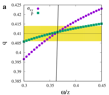
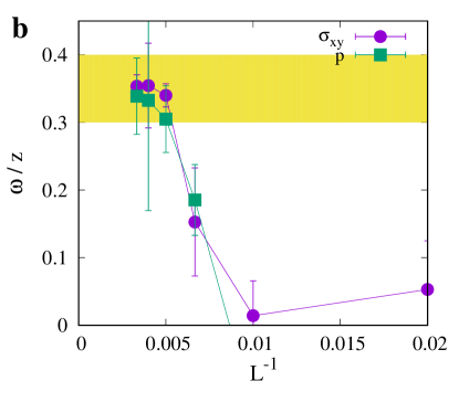
Figure 4: Matching rule. (a) Contour lines of $q$ and $\omega/z$ for $p$ and $\sigma$. The matching rule selects critical exponents where the contour lines of $p$ and $\sigma$ intersect. (b) We hold fixed $q\left(L=\infty\right)=0.41$ and obtain correction-to-scaling exponent $\omega/z$ via fitting through Eq. 7. The obtained value of $\omega/z\left(L\right)$ is plotted against $L^{-1}$. One can see that $\omega/z$ saturates for large system sizes to $\omega/z\left(L=\infty\right)=0.35$.

Exponent	$q$	$\omega/z$
$\sigma,p$	$0.410(5)$	$0.35(5)$

Table 2: Exponents. Numerical values of critical exponents.

V Discussion and conclusion

Soft spheres flow freely in a dilute regime and become amorphous solid in a dense regime. This accounts for a large range of phenomena such as jamming and glass transition. Determinations of both the transition density and exponents describing scaling near the transition point are subjects of intense research. However, because of a lack of a general framework, no consensus has yet emerged. Here, we close this debate by presenting a framework to precisely compute the exponents of the rigidity transition in soft spheres based on an accurate determination of the transition density. Furthermore, we demonstrate that even though the transition density can be uniquely determined, there is a spectrum of different numerical values for critical exponents. Thanks to isotropic asymptotic scaling of the components of the stress tensor, we introduce a matching rule that selects critical exponents and rules out other possibilities. The matching rule considers the intersection of contour lines of exponents of pressure and shear stress. This allowed us to unambiguously determine the asymptotic critical exponent of the shear stress and pressure. Having determined the asymptotic exponent $q$, we use finite-size scaling to determine the asymptotic value of exponent of the leading correction-to-scaling term $\omega/z$. We demonstrate that $\omega/z$ for both shear stress and pressure converges to the same value within the numerical uncertainty at the limit of large system sizes. Two mean-field type calculations for the exponents of the rigidity transition are proposed by Otsuki-Hayakawa Otsuki and Hayakawa (2009b) and DeGiuli et al. DeGiuli et al. (2015). Our results for exponents are closer to the predictions by the former.

Noticeably, we recover inertial-Bagnold scaling $p,\sigma\propto\dot{\gamma}^{2}$ at $\dot{\gamma}\to 0$ below jamming. This is a direct result of the fact that our dissipation rule damps out the normal component of the relative velocity with respect to the contact point of two colliding particles. However, since in a shear flow the main contribution to the kinetic energy of particles comes from the tangential relative velocities of particles, after a collision particles maintain their motion due to the apparent inertia. This fact was first noted by Refs. Vagberg et al. (2014b); DeGiuli et al. (2015).

Even though the critical density is not strongly influenced by finite size effects in our analysis, we observe a strong dependence of the critical exponents on the system size. This is a crucial point that has been overlooked in many recent studies about glass transition and jamming. In these studies, extremely small system sizes, in the order of $10^{3}$ particles, are considered. Our results indicate that such small system sizes are strongly influenced by finite size effects.

Our framework provides grounds for several immediate investigations that will deepen our understanding of amorphous materials using rheology as the main tool:

1. Critical exponents of a phase transition can be influenced by fluctuations and thus the dimensionality of the system. However, these exponents do not significantly change above a critical dimension, known as the upper critical dimension $d_{UC}$. Below this dimension, fluctuations are important. Above $d_{UC}$, fluctuations are washed out and critical exponents are equal to the mean-field exponents. The exact determination of $d_{UC}$ for the jamming transition has been a challenge: the absence of a mean field theory and the lack of a framework for the precise measurement of critical exponents can be considered as the main reasons. Many authors have suggested that $d_{UC}=2$ and that logarithmic corrections-to-scaling are involved O’Hern et al. (2003); Wyart et al. (2005); Goodrich et al. (2012, 2014, 2016). The main reason for this is that critical exponents appear to be the same for $d=2$ and $3$. Collapse of the data has been used widely in these studies to measure critical exponents. Our general approach can be easily applied in accurately measuring critical exponents in three dimensions. Then, a comparison of critical exponents at $d=2$ and $3$ can resolve the controversy over the upper critical dimension for jamming. This will be a great step ahead in understanding the nature of the jamming transition.

2. Amorphous solids possess a complex free-energy landscape Charbonneau et al. (2014). As one increases density, an amorphous solid undergoes a sequence of transitions: glass transition, Gardner transition, and jamming. Annealing has been the essential method to investigate these transitions. Standard rheological techniques have been shown to be powerful tools to investigate complex properties of this energy landscape of amorphous materials Jin and Yoshino (2017). We expect the generalization of our approach to shed light on and help formulate a general formalism to investigate other types of transitions in amorphous materials using rheology.

3. An investigation of periodically driven colloidal suspensions provided remarkable insights into the nature of rheological phase transitions. In a dilute regime, these systems undergo a non-equilibrium phase transition into an absorbing state where particles self-organize themselves to prevent collisions Pine et al. (2005); Corte et al. (2008). In the dense regime, a yielding transition, which describes the onset of plastic deformation, has been shown to be a non-equilibrium phase transition from reversibility in an elastic regime into irreversibility in a plastic regime Nagamanasa et al. (2014). Nonetheless, the nature of the transition has been disputed, including whether it is a first-order or second-order transition Regev et al. (2015); Leishangthem et al. (2017), as well as whether the absorbing state transition belongs to the universality class of (conserved) directed percolation Nagamanasa et al. (2014). In both the dilute and dense regimes, divergences of time and length scales have been reported upon approaching a critical shearing strain. However, a precise determination of the universality classes of these non-equilibrium phase transitions have not been conclusive due to the lack of a comprehensive framework for measuring critical exponents from rheological experiments Tjhung and Berthier (2015); Pine et al. (2005); Corte et al. (2008); Nagamanasa et al. (2014); Jeanneret and Bartolo (2014). Our formalism may shed light on resolving the dispute over the nature of rheological phase transitions in oscillatory shearing.

Rheological phase transitions are fascinating novel transitions, and the exploration of their characteristics provides new insights into the less-explored realm of athermal non-equilibrium phase transitions Hinrichsen (2000); Rácz (2002). Compared to other well-established equilibrium transitions, rheological phase transitions are in their infancy. We hope that our framework can aid in a better understanding of their nature.

Acknowledgments. The authors thank the Korea Institute for Advanced Study for providing computing resources (KIAS Center for Advanced Computation - Linux cluster system) for this work, and especially consultations from Hoyoung Kim. We appreciate enlightening discussions with Abbas Ali Saberi, Takahiro Hatano, Peter Olsson, and Hisao Hayakawa. This work is supported in part by the NRF grant No. 2017R1D1A1B06035497.

VI Appendix A: simulations

Numerical simulations. We perform constant volume molecular dynamics simulations of two-dimensional frictionless bidisperse disks. Interactions between particles are modeled by a linear dashpot model. Two particles $i$ and $j$ of radii $R_{i}^{a}$ and $R_{j}^{b}$ (where $a,b=0$ and $1$ stand for two different radii of bidisperse particles) at positions ${\bf r}_{i}$ and ${\bf r}_{j}$ interact when $\xi_{ij}=R_{i}^{a}+R_{j}^{b}-r_{ij}>0$. Here, $\xi_{ij}$ is called the mutual compression of particles $i$ and $j$, $r_{ij}=|{\bf r}_{i}-{\bf r}_{j}|$. The particles interact via a linear dashpot model, $F_{ij}=Y\xi_{ij}+\gamma\frac{d\xi_{ij}}{dt}$, where $Y$ and $\gamma$ are denoted as elastic and dissipative constants, respectively. Throughout the study, we adopt unitary scale $Y=1$ and $\gamma=1$, respectively.

To prevent crystallization, we use a $1:1$ binary mixture of particles where the ratio of the radii of large and small particles is set to $R^{1}/R^{0}=1.4$. The diameter of small particles is chosen as the unit of the length $2R^{0}=1$, and the mass of each particle is equal to its area, $m_{a}=\pi[R^{a}]^{2}$.

Lees-Edwards boundary conditions are applied along the ${y}$-direction. They create a uniform overall shear rate, $\dot{\gamma}$. We use LAMMPS for our simulations. Thanks to the developer team of LAMMPS, we were provided with a new version of LAMMPS that prevents artificial attractive forces arising from the dashpot model. The version can be accessed via the mailing list of LAMMPS.

We used several system sizes, the smallest $L=50$ and the largest $L=300$. We change the packing fraction by changing the number of particles $N$ via:

$$N=\frac{8}{\pi}\frac{L^{2}}{1^{2}+1.4^{2}}\phi,$$ (10)

where $1$ and $1.4$ are the diameters of small and large particles, respectively. For shear rate $\dot{\gamma}$ in the range $10^{-4}$ and $10^{-5}$, the total strain is $\gamma=30L$ and the integration time step is $dt=0.1$. For the next smaller decade, the integration time step is $dt=0.2$.

VII Appendix B: scaling ansatz

Here, we explain a formalism for deriving the scaling ansatz for a rigidity transition. The formalism in principle can be applied to any transition that is accompanied by a diverging length scale $\xi$. Upon approaching the dense regime, the motion of particles becomes coordinated. This signals the growing length scale, which diverges at the critical density $\phi_{J}$. This divergence is described by exponent $\nu$ via:

$$\xi\propto\delta\phi^{-\nu}.$$ (11)

In the proximity of a critical point, the only fundamental length scale $b$ is the correlation length scale, $b=\xi$. Eq. 11 can be cast into a dimensionless number as

$$\Pi_{\phi}=\delta\phi b^{1/\nu}.$$ (12)

The critical point is at $\delta\phi=0$ and $\dot{\gamma}\to 0$, therefore at $\delta\phi=0$, the correlation length diverges upon decreasing the shear rate:

$$\xi\propto\dot{\gamma}^{-1/z},$$ (13)

where $z$ is the dynamic exponent. This equation can be similarly cast into another dimensionless number via

$$\Pi_{\dot{\gamma}}=\dot{\gamma}b^{z}.$$ (14)

Now, any physical quantity such the shear stress $\sigma$ also scales with the distance from jamming $\sigma\propto\delta\phi^{y}$ at $\dot{\gamma}\to 0$. Combining this relation with Eq. 11 gives:

$$\sigma\propto b^{-y/\nu},$$ (15)

which provides the dimensionless number for this quantity

$$\Pi_{\sigma}=\sigma b^{y/\nu}.$$ (16)

Since $\sigma$ depends on both $\delta\phi$ and $\dot{\gamma}$

$$\Pi_{\sigma}=\mathbb{F}_{0}\left(\Pi_{\delta\phi},\Pi_{\dot{\gamma}}\right),$$ (17)

which results in

$$\sigma b^{y/\nu}=\mathbb{F}_{0}\left(\delta\phi b^{1/\nu},\dot{\gamma}b^{z}\right),$$ (18)

This is the dimensionless equation of state.

In the renormalization group method, the domain over the correlated particles are rescaled. After renormalization, the system becomes smaller by a factor of $b$ and therefore $\xi^{\prime}=\xi/b$. As a result of this, the system moves away from the critical point by renormalization. In this process, all observables and control parameters scale with distance from critical point $b$. Equation 18 describes all such scaling behaviors. Two approaches, the intermediate asymptotic approach described by dimensionless numbers and the renormalization group, arrive at similar results Goldenfeld et al. (1989).

If we choose the length scale $b$ such that $\dot{\gamma}b^{z}=1$, then

$$\sigma=\dot{\gamma}^{y/z\nu}\mathbb{F}_{1}\left(\frac{\delta\phi}{\dot{\gamma}^{1/z\nu}}\right),$$ (19)

which is the leading scaling term. At $\delta\phi=0$, $\sigma\propto\dot{\gamma}^{q}$, thus $q/y=1/z\nu$. This equation describes $\sigma$ infinitesimally close to the critical point at $\delta\phi=0$ and $\dot{\gamma}=0$.

The jamming point is characterized by two principal directions given by $\delta\phi$ and $\dot{\gamma}$. Each direction is accompanied by a principal exponent: $y$ and $q$. Near the critical point only these relevant quantities affects the dynamics. However, off the critical point, some irrelevant parameters, $w$, may affect the dynamics. Since this quantity is irrelevant, one cannot bring the system into the critical point by varying such a quantity. This means that the correlation length does not diverge if $w\to 0$. However, it may retain a scaling form near the critical region

$$\xi\propto w^{1/\omega},$$ (20)

which results to

$$\Pi_{w}=wb^{-\omega}.$$ (21)

Inserting this dimensionless number into Eq. 18 results in

$$\sigma b^{y/\nu}=\mathcal{F}_{0}\left(\delta\phi b^{1/\nu},\dot{\gamma}b^{z},wb^{-\omega}\right).$$ (22)

With $\dot{\gamma}b^{z}=1$, we arrive at

$$\sigma=\dot{\gamma}^{y/z\nu}\mathcal{F}_{1}\left(\frac{\delta\phi}{\dot{\gamma}^{1/z\nu}},w\dot{\gamma}^{\omega/z}\right),$$ (23)

A Taylor expansion of this equation to the first order gives:

$$\sigma=\dot{\gamma}^{y/z\nu}\left[\mathcal{F}_{1}^{(0)}\left(\frac{\delta\phi}{\dot{\gamma}^{1/z\nu}}\right)+\dot{\gamma}^{\omega/z}\mathcal{F}_{1}^{(1)}\left(\frac{\delta\phi}{\dot{\gamma}^{1/z\nu}}\right)\right],$$ (24)

This equation describes the leading correction-to-scaling term. At $\delta\phi=0$

$$\sigma=\dot{\gamma}^{y/z\nu}\left[c_{1}+c_{2}\dot{\gamma}^{\omega/z}\right].$$ (25)

Eq. 25 can be used for scalings of the flow curve at $\phi_{J}$.

References

- Bonn et al. (2017) D. Bonn, M. M. Denn, L. Berthier, T. Divoux, and S. Manneville, “Yield stress materials in soft condensed matter,” Rev. Mod. Phys. 89, 035005 (2017).
- Petekidis et al. (2004) G. Petekidis, D. Vlassopoulos, and P. N. Pusey, “Yielding and flow of sheared colloidal glasses,” J. Phys.: Condens. Matter 16, S3955 (2004).
- Liu and Nagel (1998) A. J. Liu and S. R. Nagel, “Nonlinear dynamics: Jamming is not just cool any more,” Nature 396, 21 (1998).
- Paredes et al. (2013) J. Paredes, M. A. J. Michels, and D. Bonn, “Rheology across the zero-temperature jamming transition,” Phys. Rev. Lett. 111, 015701 (2013).
- Trappe et al. (2001) V. Trappe, V. Prasad, L. Cipelletti, P. N. Segre, and D. A. Weitz, “jamming phase diagram for attractive particles,” Nature 411, 772 (2001).
- Rahbari et al. (2013) S. H. E. Rahbari, M. Khadem-Maaref, and S. K. A. Seyed Yaghoubi, “Universal features of the jamming phase diagram of wet granular materials,” Phys. Rev. E 88, 042203 (2013).
- Barnes and Walters (1985) H. A. Barnes and K. Walters, “The yield stress myth?” Rheologica acta 24, 323–326 (1985).
- Moeller et al. (2009) P. C. F. Moeller, A. Fall, and D. Bonn, “Origin of apparent viscosity in yield stress fluids below yielding,” Europhys. Lett. 87, 38004 (2009).
- Olsson and Teitel (2011) P. Olsson and S. Teitel, “Critical scaling of shearing rheology at the jamming transition of soft-core frictionless disks,” Phys. Rev. E 83, 030302 (2011).
- Lerner et al. (2012) E. Lerner, G. Düring, and M. Wyart, “A unified framework for non-Brownian suspension flows and soft amorphous solids,” Proc. Nat. Acad. Sc. 109, 4798 (2012).
- Kawasaki et al. (2015) T. Kawasaki, D. Coslovich, A. Ikeda, and L. Berthier, “Diverging viscosity and soft granular rheology in non-Brownian suspensions,” Phys. Rev. E 91, 012203 (2015).
- Schall and van Hecke (2010) P. Schall and M. van Hecke, “Shear bands in matter with granularity,” Annu. Rev. Fluid Mech. 42 (2010).
- Hatano (2008) T. Hatano, “Scaling properties of granular rheology near the jamming transition,” J. Phys. Soc. Jpn. 77, 12 (2008).
- Otsuki and Hayakawa (2009a) M. Otsuki and H. Hayakawa, “Universal scaling for the jamming transition,” Prog. of Theor. Phys. 121, 647–655 (2009a).
- Hatano (2010) T. Hatano, “Critical scaling of granular rheology,” Progr. Theor. Exp. Phys. 184, 143 (2010).
- Otsuki and Hayakawa (2012) M. Otsuki and H. Hayakawa, “Rheology of sheared granular particles near jamming transition,” Prog. of Theor. Phys. Supp. 195, 129–138 (2012).
- DeGiuli et al. (2015) E. DeGiuli, G. Düring, E. Lerner, and M. Wyart, “Unified theory of inertial granular flows and non-Brownian suspensions,” Phys. Rev. E 91, 062206 (2015).
- Vagberg et al. (2016) D. Vagberg, P. Olsson, and S. Teitel, “Critical scaling of Bagnold rheology at the jamming transition of frictionless two-dimensional disks,” Phys. Rev. E 93, 052902 (2016).
- Vagberg et al. (2014a) D. Vagberg, P. Olsson, and S. Teitel, “Dissipation and rheology of sheared soft-core frictionless disks below jamming,” Phys. Rev. Lett. 112, 208303 (2014a).
- Olsson and Teitel (2012) P. Olsson and S. Teitel, “Herschel-bulkley shearing rheology near the athermal jamming transition,” Phys. Rev. Lett. 109, 108001 (2012).
- Vagberg et al. (2014b) D. Vagberg, P. Olsson, and S. Teitel, “Universality of jamming criticality in overdamped shear-driven frictionless disks,” Phys. Rev. Lett. 113, 148002 (2014b).
- Radjai and Rou (2002) F. Radjai and S. Rou, “Turbulentlike fluctuations in quasistatic flow of granular media,” Phys. Rev. Lett. 89, 064302 (2002).
- Olsson (2015) P. Olsson, “Relaxation times and rheology in dense athermal suspensions,” Phys. Rev. E 91, 062209 (2015).
- Nordstrom et al. (2010) K. N. Nordstrom, E. Verneuil, P. E. Arratia, A. Basu, Z. Zhang, A. G. Yodh, J. P. Gollub, and D. J. Durian, “Microfluidic rheology of soft colloids above and below jamming,” Phys. Rev. Lett. 105, 175701 (2010).
- Olsson and Teitel (2007) P. Olsson and S. Teitel, “Critical scaling of shear viscosity at the jamming transition,” Phys. Rev. Lett. 99, 178001 (2007).
- Kardar (2007) M. Kardar, Statistical physics of fields (Cambridge University Press, 2007).
- Hayakawa and Otsuki (2013) H. Hayakawa and M. Otsuki, “Critical behaviors of sheared frictionless granular materials near the jamming transition,” Phys. Rev. E 88, 032117 (2013).
- Goodrich et al. (2016) C. P. Goodrich, A. J. Liu, and J. P. Sethna, “Scaling ansatz for the jamming transition,” Proc. Nat. Acad. Sc. 113, 9745 (2016).
- Maloney and Lemaître (2006) C. E. Maloney and A. Lemaître, “Amorphous systems in athermal, quasistatic shear,” Phys. Rev. E 74, 016118 (2006).
- Bouchbinder et al. (2007) E. Bouchbinder, J. S. Langer, and I. Procaccia, “Athermal shear-transformation-zone theory of amorphous plastic deformation. i. basic principles,” Phys. Rev. E 75, 036107 (2007).
- Lemaitre and Caroli (2009) A. Lemaitre and C. Caroli, “Rate-dependent avalanche size in athermally sheared amorphous solids,” Phys. Rev. Lett. 103, 065501 (2009).
- Hentschel et al. (2010) H. G. E. Hentschel, S. Karmakar, E. Lerner, and I. Procaccia, “Size of plastic events in strained amorphous solids at finite temperatures,” Phys. Rev. Lett. 104, 025501 (2010).
- Hatano et al. (2015) T. Hatano, C. Narteau, and P. Shebalin, “Common dependence on stress for the statistics of granular avalanches and earthquakes,” Sci. Rep. 5 (2015).
- Nicolas et al. (2017) A. Nicolas, E. E. Ferrero, K. Martens, and J. L. Barrat, “Deformation and flow of amorphous solids: a review of mesoscale elastoplastic models,” arXiv:1708.09194 (2017).
- Landau and Lifshitz (1986) L. D. Landau and E. M. Lifshitz, “Theory of elasticity, vol. 7,” Course of Theoretical Physics 3, 109 (1986).
- Peyneau and Roux (2008) P. E. Peyneau and J. N. Roux, “Solidlike behavior and anisotropy in rigid frictionless bead assemblies,” Phys. Rev. E 78, 041307 (2008).
- Baity-Jesi et al. (2017) M. Baity-Jesi, C. P. Goodrich, A. J. Liu, S. R. Nagel, and J. P. Sethna, “Emergent so3 symmetry of the frictionless shear jamming transition,” J. Stat. Phys. 167, 735–748 (2017).
- Vagberg et al. (2017) D. Vagberg, P. Olsson, and S. Teitel, “Effect of collisional elasticity on the bagnold rheology of sheared frictionless two-dimensional disks,” Phys. Rev. E 95, 012902 (2017).
- Suzuki and Hayakawa (2017) K. Suzuki and H. Hayakawa, “Theory for the rheology of dense non-brownian suspensions: divergence of viscosities and - rheology,” arXiv:1711.08855 (2017).
- Heussinger and Barrat (2009) C. Heussinger and J. L. Barrat, “Jamming transition as probed by quasistatic shear flow,” Phys. Rev. Lett. 102, 218303 (2009).
- O’Hern et al. (2003) C.S. O’Hern, L.E. Silbert, A.J. Liu, and S.R. Nagel, “Jamming at zero temperature and zero applied stress: The epitome of disorder,” Phys. Rev. E 68, 011306 (2003).
- Otsuki and Hayakawa (2009b) M. Otsuki and H. Hayakawa, “Critical behaviors of sheared frictionless granular materials near the jamming transition,” Phys. Rev. E 80, 011308 (2009b).
- Wyart et al. (2005) M. Wyart, L. E. Silbert, S. R. Nagel, and T. A. Witten, “Effects of compression on the vibrational modes of marginally jammed solids,” Phys. Rev. E 72, 051306 (2005).
- Goodrich et al. (2012) C. P. Goodrich, A. J. Liu, and S. R. Nagel, “Finite-size scaling at the jamming transition,” Phys. Rev. Lett. 109, 095704 (2012).
- Goodrich et al. (2014) C. P. Goodrich, S. Dagois-Bohy, B. P. Tighe, M. van Hecke, A. J. Liu, and S. R. Nagel, “Jamming in finite systems: Stability, anisotropy, fluctuations, and scaling,” Phys. Rev. E 90, 022138 (2014).
- Charbonneau et al. (2014) P. Charbonneau, J. Kurchan, G. Parisi, P. Urbani, and F. Zamponi, “Fractal free energy landscapes in structural glasses,” Nat. Commun. 5, 3725 (2014).
- Jin and Yoshino (2017) Y. Jin and H. Yoshino, “Exploring the complex free-energy landscape of the simplest glass by rheology,” Nat. Commun. 8, 14935 (2017).
- Pine et al. (2005) D. J. Pine, J. P. Gollub, J. F. Brady, and A. M. Leshansky, “Chaos and threshold for irreversibility in sheared suspensions,” Nature 438, 997 (2005).
- Corte et al. (2008) L. Corte, P. M. Chaikin, J. P. Gollub, and D. J. Pine, “Random organization in periodically driven systems,” Nature Phys. 4, 420 (2008).
- Nagamanasa et al. (2014) K. H. Nagamanasa, S. Gokhale, A. K. Sood, and R. Ganapathy, “Experimental signatures of a nonequilibrium phase transition governing the yielding of a soft glass,” Phys. Rev. E 89, 062308 (2014).
- Regev et al. (2015) I. Regev, J. Weber, C. Reichhardt, K. A Dahmen, and T. Lookman, “Reversibility and criticality in amorphous solids,” Nat. Commun. 6, 8805 (2015).
- Leishangthem et al. (2017) P. Leishangthem, A. D. S. Parmar, and S. Sastry, “The yielding transition in amorphous solids under oscillatory shear deformation,” Nat. Commun. 8, 14653 (2017).
- Tjhung and Berthier (2015) E. Tjhung and L. Berthier, “Hyperuniform density fluctuations and diverging dynamic correlations in periodically driven colloidal suspensions,” Phys. Rev. Lett. 114, 148301 (2015).
- Jeanneret and Bartolo (2014) R. Jeanneret and D. Bartolo, “Geometrically protected reversibility in hydrodynamic loschmidt-echo experiments,” Nat. Commun. 5, 3474 (2014).
- Hinrichsen (2000) Haye Hinrichsen, “Non-equilibrium critical phenomena and phase transitions into absorbing states,” Adv. Phys. 49, 815 (2000).
- Rácz (2002) Z. Rácz, “Nonequilibrium phase transitions,” arXiv preprint cond-mat/0210435 (2002).
- Goldenfeld et al. (1989) N. Goldenfeld, O. Martin, and Y. Oono, “Intermediate asymptotics and renormalization group theory,” J. Sci. Comput. 4, 355–372 (1989).