The UVES Spectral Quasar Absorption Database (SQUAD) Data Release 1: The first 10 million seconds

Abstract

We present the first data release (DR1) of the UVES Spectral Quasar Absorption Database (SQUAD), comprising 467 fully reduced, continuum-fitted high-resolution quasar spectra from the Ultraviolet and Visual Echelle Spectrograph (UVES) on the European Southern Observatory’s Very Large Telescope. The quasars have redshifts $z=0$–5, and a total exposure time of 10 million seconds provides continuum-to-noise ratios of 4–342 (median 20) per 2.5-$\textrm{km\,s}^{-1}$ pixel at 5500 Å. The SQUAD spectra are fully reproducible from the raw, archival UVES exposures with open-source software, including our uves_popler tool for combining multiple extracted echelle exposures which we document here. All processing steps are completely transparent and can be improved upon or modified for specific applications. A primary goal of SQUAD is to enable statistical studies of large quasar and absorber samples, and we provide tools and basic information to assist three broad scientific uses: studies of damped Lyman-$\alpha$ systems (DLAs), absorption-line surveys and time-variable absorption lines. For example, we provide a catalogue of 155 DLAs whose Lyman-$\alpha$ lines are covered by the DR1 spectra, 18 of which are reported for the first time. The H i column densities of these new DLAs are measured from the DR1 spectra. DR1 is publicly available and includes all reduced data and information to reproduce the final spectra.

1 Introduction

The era of 8-and-10-metre telescopes has revolutionised the study of quasar absorption spectra. Before the Keck I 10-metre telescope’s first light with the High Resolution Echelle Spectrometer in 1993 (HIRES; Vogt et al., 1994), few quasars were bright enough to be studied with reasonable signal-to-noise ratio (S/N) at resolving powers $R\gtrsim 40000$ with smaller telescopes. This new reach was extended to the southern hemisphere in 1999 with the Ultraviolet and Visual Echelle Spectrograph (UVES; Dekker et al., 2000) on the European Southern Observatory’s (ESO’s) 8-metre Very Large Telescope (VLT).

Since its commissioning, UVES has contributed to a wide variety of extragalactic discoveries and studies, particularly using absorption lines arising in gas clouds along quasar sight-lines. For example, UVES spectra have been used to trace the metallicity, power-spectrum and thermal history of the intergalactic medium via $\textrm{Ly-}\alpha$ forest absorption lines (e.g. Schaye et al., 2003; Kim et al., 2004; Boera et al., 2014). The chemical abundances of circumgalactic environments, traced by the highest-column density clouds – the damped $\textrm{Ly-}\alpha$ systems (DLAs) and sub-DLAs – have been studied in detail with UVES (e.g Molaro et al., 2000; Pettini et al., 2002; Pettini et al., 2008a; Dessauges-Zavadsky et al., 2003). UVES spectra have also been used to discover and analyse molecular hydrogen and carbon monoxide in (sub-)DLAs (e.g. Ledoux et al., 2003; Noterdaeme et al., 2008; Srianand et al., 2008) and, recently, in likely examples of the high-redshift interstellar medium (e.g. Noterdaeme et al., 2015, 2017). Measurements of key cosmological parameters have been made with UVES quasar spectra; for example, deuterium abundance constraints on the total energy density of baryons (e.g. Pettini et al., 2008b; Pettini & Cooke, 2012; Riemer-Sørensen et al., 2017) and the redshift evolution of the cosmic microwave background temperature (e.g. Noterdaeme et al., 2011). UVES quasar spectra have even been used to constrain cosmological variations in the fundamental constants of nature (e.g. Quast et al., 2004; King et al., 2008; King et al., 2012; Rahmani et al., 2013; Molaro et al., 2013; Murphy et al., 2016).

It is notable that most of the above studies utilised a UVES spectrum of a single quasar. While this demonstrates the high scientific value of such spectra, large samples are often required to enable some scientific projects, to make a meaningful measurement or improvement over previous ones. One difficulty is that reducing raw high-resolution (i.e. echelle) spectroscopic data is challenging and can require considerable experience, even with observatory-supplied data reduction pipelines. Combining the spectra from many quasar exposures and continuum-fitting the final spectrum are almost always required, but these steps are not straight-forward and usually fall outside the scope of reduction pipelines. Therefore, most studies using UVES quasar spectra have not made general-purpose, combined spectra publicly available. Doing so can be time-consuming and low priority compared to the immediate, specific scientific purpose for which the UVES observations were proposed. This has severely limited the availability and use of large samples of high-resolution quasar spectra.

Considerable efforts have already been invested to address these limitations: Zafar et al. (2013a) presented a database of 250 UVES quasar spectra and O’Meara et al. (2015); O’Meara et al. (2017) has provided 300 HIRES quasar spectra. To further assist, we provide here the UVES Spectral Quasar Absorption Database (SQUAD) first data release (DR1): 467 “science-ready” UVES quasar spectra at redshifts $z_{\textrm{\scriptsize em}}=0$–5. Importantly, the processing steps for each quasar spectrum in DR1 are fully transparent and repeatable. That is, all the steps to reduce and combine the multiple exposures of a quasar, and “clean” and continuum fit its combined spectrum, are fully visible and can be repeated by executing a few commands using public, open-source software. This end-to-end transparency and reproducibility ensures that scientific applications for which certain aspects of the data are important (e.g. the wavelength calibration accuracy) have an unbroken record of their treatment, from raw data to final, combined spectrum. Our public software ensures that each spectrum can be improved by its users as it is employed for different purposes (each with a different scientific focus), or modified to suit a particular scientific application, and that all changes can easily be made transparent and reproducible to others. We have also attempted to process the DR1 spectra as uniformly as possible so they may be most useful for statistical studies of large quasar samples.

The UVES SQUAD differs in several ways from the database of Zafar et al. (2013a). The latter drew on ESO’s Advanced Data Products (ADP) archive: automatic reductions of point-source exposures, in settings for which standardised (“master”) calibration files were available. This used the original eso-midas data reduction pipeline which has now been superseded by a pipeline with superior spectral extraction quality and which we optimise for better wavelength calibration accuracy. Zafar et al. combined the ADP-reduced exposures of a quasar using custom software. Our experience suggests that this processes can be very important, even critical, for some scientific applications, which further motivates our fully transparent and reproducible approach, and the ability for users to modify the parameters of the reduction and/or combination process easily. Finally, the ADP-reduced exposures are redispersed (re-gridded) onto a linear wavelength grid. Given that UVES is a grating cross-dispersed echelle, the resolving power does not vary strongly with wavelength, so a linear wavelength grid is inappropriate: it will undersample the resolution element at the bluest wavelengths and/or oversample it at the reddest wavelengths. Further, combining multiple exposures onto a common wavelength grid entails redispersing them again (e.g. to accommodate different heliocentric velocities). This introduces further correlations between the flux (and uncertainty) in neighbouring pixels, and slightly lowers the resolving power. We avoid these problems in the UVES SQUAD by reducing the raw data and redispersing all extracted exposures once to a common log-linear, vacuum–heliocentric grid. Combining all (extracted) exposures in this way provides the highest S/N, highest-resolution, appropriately sampled final spectrum of each quasar.

This paper is organised as follows. Section 2 describes how DR1 is defined, how the quasars were identified in ESO’s UVES data archive, and presents the DR1 quasar catalogue (Table 1). Section 3 details how appropriate calibration data were identified for each quasar exposure, and the data reduction process. Section 4 documents our uves_popler software for combining multiple (extracted) UVES exposures of a quasar to produce the “science-ready”, final DR1 spectra. Section 5 describes the basic properties of the DR1 spectra and the main remaining artefacts that most or all spectra contain. In Section 6 we illustrate three examples of the many applications for the DR1 sample: DLA studies, absorption-line surveys and studies of time-variable absorption lines. In particular, we present a catalogue of 155 DLAs where the $\textrm{Ly-}\alpha$ line is covered by the DR1 spectra, 18 of which have not been reported before. We measure H i column densities for these new DLAs directly from the DR1 spectra. Section 7 summarises the paper and discusses future SQUAD data releases.

The DR1 database, including all reduced data and files required to produce the final DR1 spectra, are publicly available in Murphy et al. (2018).

2 Quasar selection and catalogue

Table 1 catalogues the DR1 quasar and spectrum properties. This first data release is defined as containing the 475 quasars in the ESO UVES archive whose first exposure (longer than 100 s) was observed before 30th June 2008. All exposures of these quasars (longer than 100 s) observed before 17th November 2016 were included in the final, combined spectra in DR1. In total, 3088 exposures were selected and successfully processed, with a total exposure time of $10.09\times 10^{6}$ s (2803 h, an average of 5.9 h per quasar).

The quasar candidates satisfying these date criteria were selected by cross-matching the coordinates of all “science” observations in the ESO UVES archive (i.e. with DPR.CATG set to “SCIENCE”) with the MILLIQUAS quasar catalogue (Flesch, 2015, updated to version 5.2). While this catalogue aims to include all quasars from the literature (up to August 2017), it will not include unpublished quasars. To identify such cases, we checked the ESO proposal titles and observed object names (as labelled by the observers) for all programs that observed any MILLIQUAS quasar with UVES and searched for any objects observed in those programs that may be quasars (and not already reported in MILLIQUAS). This approach identified 9 of the final 475 quasars selected for DR1, and a further 18 objects that, upon data reduction and exposure combination, were clearly not quasars (17 stars and one galaxy). While it is possible that some quasars were not selected by our approach, our manual checking of the proposal titles and object names should ensure this number is very small or zero.

All quasar candidates were identified in the SuperCosmos Sky Survey database (Hambly et al., 2001) to determine a complete set of J2000 coordinates. In cases where a spectrum is available from the Sloan Digital Sky Survey

Table 1: The UVES SQUAD DR1 sample of 475 quasars, of which we provide final spectra for 467. The first 20 columns provide the quasar names, coordinates, redshifts and optical/infra-red photometry sourced from several databases: SDSS, SuperCosmos, NED and SIMBAD (see text). The next seven columns specify the important observational information: the number of UVES exposures, their total duration, the ESO Program IDs, the UVES wavelength settings, slit widths and on-chip binnings used, and the prevailing seeing values reported in the ESO Science Archive (when available, the minimum, median and maximum seeing are reported, and “NA” is reported when seeing information is not available). The final five columns summarise the final spectrum properties (see text for full explanations): the “Spec. status” flag indicates whether we produced a final spectrum (values 0, 1 and 2), or whether multiple objects in the slit, a lack of calibration exposures, or a very high redshift precluded this (values 3, 4 and 5); the dispersion of the final spectrum ($\textrm{km\,s}^{-1}$ per pixel); its wavelength coverage (Section 5); the continuum-to-noise ratio and nominal resolving power calculated at five representative wavelengths (see Section 5). The full table is available as Supporting Information online and contains additional information, including the DLA catalogue discussed in Section 6.1.

DR1 Name	RAAdopt	DecAdopt	$z_{\rm em,Adopt}$	SDSS Name	NED Name	SIMBAD Name	$z_{\rm em,SDSS}$	$z_{\rm em,NED}$	$z_{\rm em,SIMBAD}$	BSSS	R1SSS	R2SSS	ISSS
	(J2000)									[mag]	[mag]	[mag]	[mag]
J000149$-$015939	00:01:49.94	$-$01:59:39.4	2.815	SDSS J000149.94$-$015939.4	LBQS 2359$-$0216B	[LE2003] Q2359$-$02A	2.815	2.817	0	18.69	18.31	18.52	18.59
J000322$-$260318	00:03:22.94	$-$26:03:18.3	4.098		[HB89] 0000$-$263	QSO B0000$-$26		4.098	4.111	19.55	17.12	16.94	16.74
J000344$-$232355	00:03:44.91	$-$23:23:55.3	2.280		HE 0001$-$2340	QSO B0001$-$2340		2.280	2.280	16.75	16.69	16.47	15.93
J000443$-$555044	00:04:43.28	$-$55:50:44.6	2.100							18.37	18.01	17.50	17.06
J000448$-$415728	00:04:48.27	$-$41:57:28.1	2.760		TOLOLO 0002$-$422	QSO B0002$-$4214		2.760	2.760	17.91	17.45	17.14	16.86
J000651$-$620803	00:06:51.62	$-$62:08:03.3	4.455		BR J0006$-$6208	QSO B0004$-$6224		4.455	4.455	21.62	18.70	19.04	18.06
J000815$-$095854	00:08:15.33	$-$09:58:54.3	1.955	SDSS J000815.33$-$095854.3	SDSS J000815.33$-$095854.0	SDSS J000815.33$-$095854.3	1.955	1.95	1.951	18.33	18.24	17.92	17.53
J000852$-$290043	00:08:52.70	$-$29:00:43.7	2.645		2QZ J000852.7$-$290044	QSO B0006$-$2917		2.645	2.645	19.16	18.27	18.17	17.93
J000857$-$290126	00:08:57.72	$-$29:01:26.4	2.607		2QZ J000857.7$-$290126	QSO B0006$-$2918		2.607	2.607	19.93	19.34	19.41	19.06
J001130$+$005550	00:11:30.55	$+$00:55:50.8	2.290	SDSS J001130.55$+$005550.8	[HB89] 0008$+$006	[HHB2004] A1	2.290	2.309	2.291	19.16		18.43	17.69

$u_{\rm SDSS}$	$g_{\rm SDSS}$	$r_{\rm SDSS}$	$i_{\rm SDSS}$	$z_{\rm SDSS}$	Num.	Exp. Time	ESO Program IDs	Wavelength settings	Slit widths	Binnings	Seeing	Spec.	Disper-
					Exp.					(spec. $\times$ spat.)	(min., med., max.)	status	sion
[mag]	[mag]	[mag]	[mag]	[mag]		[s]		[nm]	[arcsec]		[arcsec]		[$\textrm{km\,s}^{-1}$]
20.26	18.95	18.79	18.82	18.63	6	21300	073.B-0787(A), 66.A-0624(A)	346, 390, 437, 580, 760, 860	0.9, 1.0	2$\times$2	0.56, 1.50, 2.03	0	2.5
					4	16100	60.A-9022(A)	437, 860	0.9	2$\times$2	0.34, 0.49, 1.97	1, 2	2.5
					26	108482	083.A-0733(A), 083.A-0733(I), 166.A-0106(A)	346, 390, 420, 437, 580, 700, 760, 860	0.7, 1.0	1$\times$1, 2$\times$2	0.40, 0.94, 2.20	0	1.3
					7	21288	074.A-0473(A)	390, 564	0.8	2$\times$2	0.61, 1.24, 2.28	0	2.5
					46	178664	166.A-0106(A), 185.A-0745(C), 185.A-0745(F)	346, 390, 437, 564, 580, 760, 860	0.8, 1.0	1$\times$1, 2$\times$2	0.37, 0.80, 2.81	0	2.0
					2	7199	69.A-0613(A)	580	1.0	2$\times$2	0.83, 1.06, 1.10	0	2.5
19.17	18.85	18.36	18.00	17.90	6	21600	076.A-0376(A)	390, 760	0.9, 1.0	2$\times$2	0.86, 1.30, 2.20	0	2.5
					6	24000	075.A-0617(A), 70.A-0031(A)	390, 437, 760, 860	1.1, 1.2	2$\times$2	0.62, 0.80, 1.09	0	2.5
					6	17700	075.A-0617(A), 70.A-0031(A)	390, 437, 760, 860	1.1, 1.2	2$\times$2	0.58, 0.95, 1.50	0	2.5
20.02	19.06	18.69	18.29	17.99	2	7200	267.B-5698(A)	437, 860	1.0	2$\times$2	NA, NA, NA	0	2.5

Wavelength coverage	Cont.-to-noise ratio at $\lambda_{\rm obs}=$	Nom. Res. Power at $\lambda_{\rm obs}=$
	3500, 4500, 5500, 6500, 7500 Å	3500, 4500, 5500, 6500, 7500 Å
[Å]		[1000]
3231–5760, 5761–…–10429	6, 12, 12, 15, 11	49.8, 49.8, 52.0, 49.9, 52.0
3952–4981, 4986–5000, 6731–8521	0, 65, 0, 0, 48	0, 54.5, 0, 0, 52.0
3064–4894, 4898–4902, 4905–4949, 4954–5235, 5241–…–10257	36, 66, 97, 106, 99	60.1, 60.1, 53.7, 53.7, 50.8
3290–4520, 4622–5600, 5675–6616, 6619–6652	22, 16, 42, 40, 0	59.8, 59.8, 56.9, 56.9, 0
3049–…–10430	49, 113, 122, 144, 101	49.8, 55.8, 47.8, 50.6, 47.8
4809–4855, 4858–5755, 5841–6802	0, 0, 18, 28, 0	0, 0, 47.8, 47.8, 0
3297–4519, 5685–5742, 5759–5826, 5829–7521, 7665–9466	11, 26, 0, 40, 42	49.8, 49.8, 0, 52.0, 52.0
3296–4984, 5678–5921, 5931–5982, 5988–…–10429	16, 165, 0, 46, 41	41.5, 41.5, 0, 41.1, 41.1
3324–4984, 5679–5745, 5760–7966, 7967–…–10434	5, 16, 0, 16, 16	41.5, 41.5, 0, 41.1, 41.1
3760–4984, 6692–6770, 6779–6921, 6929–…–10432	0, 8, 0, 0, 17	0, 49.8, 0, 0, 47.8

(SDSS DR14; Abolfathi et al., 2018; Pâris et al., 2018), the SDSS coordinates were used in preference. These coordinates were used to name all quasars in DR1; this results in the unique “DR1 Name” field for each quasar in Table 1. Quasar emission redshifts were taken from a hierarchy of cross-matched databases: SDSS, NED, SIMBAD and, if the quasar appeared in none of these databases, our own approximate measurement from our final spectrum. The latter was required in 13 cases, but in one of these (J031257$-$563912), no emission line could be identified from which a redshift could be estimated (its redshift is set to zero in Table 1). This provides a nominal, adopted redshift for each quasar, named “$z_{\rm em,Adopt}$” in Table 1. The sky position and redshift distributions of the quasars are plotted in Figure 1.

  

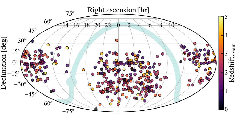
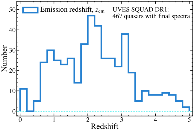
Figure 1: Left panel: Sky distribution of the 467 DR1 quasars in Table 1 for which final spectra were produced. The colour/shading of the points encodes the quasar redshift as indicated. The light blue shaded stripe and bulge represent the Galactic plane and centre. Right panel: Distribution of emission redshifts ($z_{\rm em,Adopt}$ in Table 1) for the DR1 quasars with final spectra.

DR1 contains final spectra for 467 of the 475 quasars in Table 1. Known shortcomings of the final spectrum, or the reason why one could not be produced, are encoded for each quasar in Table 1 in the “Spec. status” flag, which can have the following values:

• ${\rm Spec.\ status}=0$: A final spectrum was produced with no known problems.

• ${\rm Spec.\ status}=1$: Not all available exposures could be successfully processed for lack of appropriate calibration exposures. This applies to two quasars (J000322$-$260318 and J030722$-$494548). The wavelength coverage of their final spectra is significantly reduced as a result.

• ${\rm Spec.\ status}=2$: The wavelength calibration of at least some exposures are very obviously distorted. This applies to one quasar spectrum, J000322$-$260318; this should be used with caution.

• ${\rm Spec.\ status}=3$: Quasars at redshifts $z_{\textrm{\scriptsize em}}\geq 5.8$, so the extremely thick $\textrm{Ly-}\alpha$ forest left very little flux in individual exposures. This applies to three quasars (J130608$+$035626, J103027$+$052455, J104433$-$012502). Combining the exposures using our approach (particularly the order scaling step) is not effective in such cases (Section 4.2.2); the exposures would need to be spectrophotometrically flux calibrated to allow reliable combination.

• ${\rm Spec.\ status}=4$: More than one object with similar magnitude aligned in the slit. This applies to two lensed quasars J110633$-$182124 and J145433$-$401232. Producing separate, successfully resolved spectra would require non-standard reduction steps not implemented here. The observations of another lensed quasar, J091127$+$055054, had a second, much fainter object aligned in the slit; this did not affect the data reduction steps so we provide a final spectrum for this object but urge caution in using it.

• ${\rm Spec.\ status}=5$: A lack of appropriate calibration exposures in the ESO UVES archive precluded the basic data reduction steps required. This applies to three quasars (J030449$-$000813, J223337$-$603329, J033032$-$270438).

3 Data calibration and reduction

3.1 Science and calibration data selection

UVES is a two-arm, grating cross-dispersed echelle spectrograph mounted on the Nasmyth platform of Unit Telescope 2 of the VLT (Dekker et al., 2000). Combined, the two arms can cover a very broad wavelength range ($\sim$3050–10500 Å), albeit with gaps depending on the wavelength settings chosen. The blue arm camera contains a single CCD chip, while the red arm camera contains a two-chip mosaic. Most observations use both arms simultaneously, with the quasar light split into the two arms by a dichroic mirror, in two of nine standard wavelength settings named according to the central wavelength, in nm: 346, 390 and 437 for the blue arm; 520, 564, 580, 600, 760 and 860 for the red arm. However, some observations use a single arm only, and many different non-standard wavelength settings. The wavelength settings used for the DR1 quasar observations are specified in Table 1. Each setting is characterised by a different, nominal wavelength coverage.

We only consider exposures taken through an entrance slit; UVES has an image slicer option but we exclude such data from DR1. The slit width and on-chip binning determine the nominal resolving power, i.e. that expected for a fully illuminated slit, as is the case for ThAr exposures. However, the quasar exposure’s resolving power will be somewhat larger than this, especially if the seeing FWHM is significantly less than the slit width. Table 1 therefore provides the range of slit widths, binnings and seeing during the observations as a guide (Section 5 discusses the nominal resolving power reported in Table 1 for the final spectra). We do not include quasar observations made through UVES’s iodine absorption cell; these require additional calibration exposures and cannot be combined with non-absorption cell observations of the same quasars. Finally, we exclude exposures taken with the Fibre Large Array Multi Element Spectrograph (FLAMES) mode of UVES. Given the above spectrograph details, a range of calibration exposures are required to reduce each quasar exposure.

The default operations model for UVES is that all calibration exposures are taken in the morning after each night’s observations. This means that some exposures are used to calibrate more than one quasar exposure, and that associating calibrations with exposures requires a matching algorithm. We requested all available UVES “science” exposures of the DR1 quasars, within 1 arcminute search boxes of their adopted coordinates (from SDSS or SuperCosmos), plus matching calibration exposures, from the ESO Science Archive. However, for many quasars the calibration matching algorithm was clearly imperfect so additional, manual requests for a large number of calibration exposures around the observation dates of many quasars were made as well. This resulted in a large database of potential calibration files. We used a custom-written code, uves_headsort (Murphy, 2016a), to ensure that the best-matching calibrations were selected within a specified “calibration period” before and after each quasar exposure. This generally meant selecting the calibration exposure(s) closest in time to the corresponding quasar exposure for five different calibration types:

• Wavelength calibration: A single thorium-argon (ThAr) exposure with the same spectrograph settings (i.e. wavelength setting, on-chip binning and slit-width), was generally selected. Given the UVES operations model, in most cases the ThAr exposure was taken at least several hours after the quasar exposure. Indeed, the median time difference for all 3088 processed DR1 exposures is 5.4 h. However, preference was given to “attached” ThAr exposures, i.e. those taken immediately after quasar exposures without any grating angle changes. An attached ThAr exposure was identified as having the same grating encoder value as the corresponding quasar exposure. In a very small number of cases, particularly for exposures taken before 2001, a slightly different slit width was allowed for the matched ThAr exposure compared to the quasar exposure.

• Order format and definition: ThAr and quartz lamp exposures taken through a short slit are used to identify the echelle orders and define a baseline trace across the CCD. A single exposure of each type with the same spectrograph settings (except for the much shorter slit), was selected in all cases.

• Flat field: Five quartz lamp exposures with the same spectrograph settings were selected. In a small number of cases, especially for early UVES data (before 2003), some quasar exposures only had 3 or 4 matching flat field exposures; rarely, only a single flat field exposure could be found for quasar exposures taken before 2002.

• Bias: The five bias (zero-duration) exposures taken on the same CCD as the quasar exposure were selected in all but rare cases from early UVES operations (before 2002).

3.2 Reduction with uves_headsort and the ESO Common Pipeline Library

After determining the best set of calibration exposures for a given quasar exposure, uves_headsort outputs a reduction script for use with ESO’s Common Pipeline Library (cpl, version 4.7.8) of UVES data reduction routines, specifically via the ESO Recipe Execution Tool (esorex) command-line interface. This provides a highly streamlined data reduction pipeline – typically, a quasar exposure can be matched with calibrations and fully reduced within several minutes – while allowing low-level access to the data reduction parameters for improving the reduction if required.

Most of the reduction steps are standard for UVES data and are explained in detail in the UVES cpl pipeline manual. Briefly, these standard steps are:

1. ThAr lines are identified on the format definition frame and used to constrain a physical model of the UVES echellogram. This identifies the diffraction order numbers and spectral setup of the exposure which assists the order definition [step (ii)] and enables the automatic wavelength calibration in step (iv) below.

2. The order definition exposure is used to establish a baseline trace for object light along each echelle order. This acts as an initial guide for extracting the quasar flux.

3. The bias and flat-field exposures are combined to form masters which are used to correct the quasar exposure for bias and dark-current offsets and pixel-to-pixel sensitivity variations in the subsequent steps.

4. The ThAr flux is extracted along the default trace in the wavelength calibration exposure (corrected for the blaze function using the master flat) and the ThAr lines are automatically, iteratively matched with those in the list carefully selected for UVES in Murphy et al. (2007). This allows a polynomial (air) wavelength solution to be established for the entire CCD (i.e. air wavelength versus pixel position for each echelle order).

5. The quasar flux is optimally extracted, with weights determined by averaging the quasar flux along small spectral sections (normally 32 pixels) and either fitting a Gaussian function to this average profile or using it directly, depending on its S/N. The sky flux is extracted simultaneously in this process and is subtracted from the quasar flux in each extracted spectral pixel. The 1$\sigma$ flux uncertainty is also determined from the quasar flux, sky flux and CCD noise characteristics. The flux and uncertainty spectra are corrected for the blaze function using the master flat.

Step (iv) was then repeated for the DR1 spectra to improve their wavelength calibration. The optimal extraction weights from step (v) were used to re-extract the ThAr spectra and perform a refined wavelength calibration process. This ensures that the same pixels, with the same statistical weights, are being used to establish the wavelength scale for the quasar spectrum (e.g. it naturally negates the effects of spatially tilted ThAr lines on the CCD). uves_headsort’s reduction scripts also modify cpl’s defaults for the wavelength polynomial degree, the number of ThAr lines to search for and select before performing the iterative polynomial fitting, and the tolerance allowed between the fitted and expected wavelength of ThAr lines. Typically, these new defaults simultaneously increase the number of lines used in the wavelength calibration, reduce the residuals around the final wavelength solution, and marginally improve the accuracy of the solution (due to increasing the polynomial degree). In some cases, particularly with the very blue wavelength settings (e.g. the standard 346 and 390-nm settings), these new defaults were modified manually to achieve a more robust wavelength solution (i.e. to increase the number of ThAr lines used).

Figure 2 shows the resulting root-mean-square deviation from the mean (RMS) of the wavelength calibration residuals for each CCD chip for all DR1 quasar exposures taken with a 1-arcsecond-wide slit and 2$\times$2 on-chip binning in the six most commonly-used wavelength settings. Together, these exposures comprise 53% of all DR1 quasar exposures. In all but the bluest two settings, our approach to the wavelength calibration produced very similar residuals for almost all exposures. For the 390 and particularly the 346-nm settings, some exposures had substantially larger residuals. This is mainly due to the strong variation in UVES’s total efficiency across the wavelength ranges covered by these settings. This causes a deficiency in the number of ThAr lines found above the intensity threshold set by the cpl pipeline in the bluest orders. Although the cpl pipeline addresses this problem in most cases, in some cases the tolerance for accepting calibration lines had to be increased so that enough lines could be found to provide a robust wavelength solution. This, in turn, causes the observed increase in the RMS of the wavelength calibration residuals in such cases.

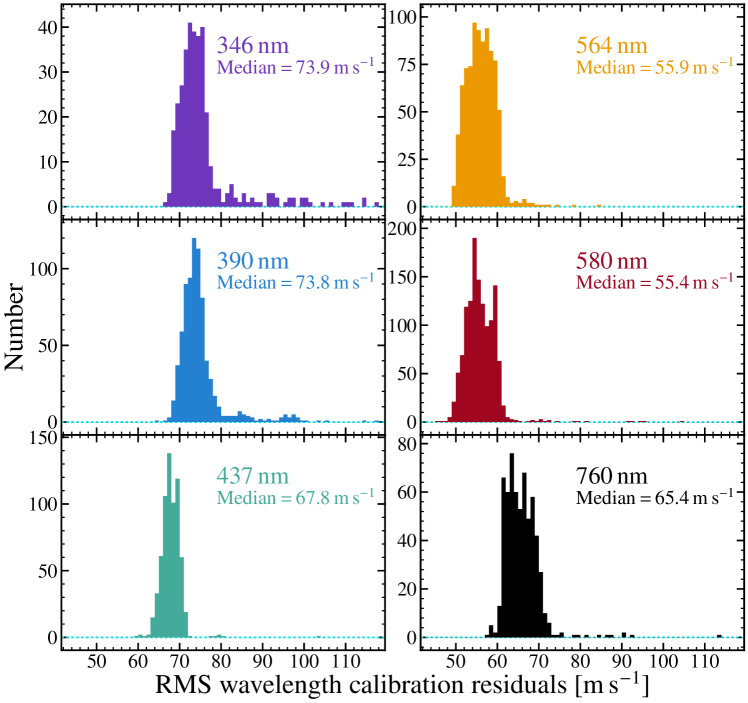
Figure 2: Typical RMS wavelength calibration residuals. The distributions show the calibration results for each DR1 quasar exposure taken with a 1-arcsecond-wide slit and 2$\times$2 on-chip binning in the six most common wavelength settings (as labelled).

After step (v) above, the cpl pipeline redisperses the flux and uncertainty arrays onto a linear wavelength grid (i.e. all pixels have the same size in wavelength), merges the spectra from adjacent spectral orders, and corrects the spectral shape using an estimate of the instrument response curve. However, because the resolving power remains reasonably constant across the wavelength range of grating cross-dispersed echelle spectrographs, and UVES covers more than a factor of three in wavelength range ($\sim$3050–10500 Å), a constant dispersion in wavelength is inappropriate; it inevitably oversamples the resolution element in the bluest parts of the spectrum and/or undersamples it in the reddest parts. Also, merging adjacent orders should account for small instrument response and/or blaze correction imperfections and variations by scaling their relative flux before averaging, but the accuracy of this is severely limited in a single exposure due to lack of S/N. However, almost all quasars in DR1 were observed in multiple exposures, so there is an opportunity to improve the merging of adjacent orders by considering all exposures together. And, finally, if the spectra from multiple exposures are to be combined, they will have to be redispersed, again, onto a common wavelength grid after correction for heliocentric motions. For these reasons, we use the not-redispersed, extracted flux and uncertainty arrays of each order (not flux calibrated), from every exposure, to produce each quasar’s final spectrum. This was performed using the custom-written code, uves_popler, described below. All relevant pipeline products are provided for every DR1 exposure in Murphy et al. (2018).

4 uves_popler: UVES Post-pipeline Echelle Reduction

uves_popler (Murphy, 2016b) was designed specifically for combining the UVES data reduction pipeline products to produce a final, continuum-fitted spectrum (however, it can also use products from many other data reduction pipelines, including those often used for Keck/HIRES and Subaru/HDS high-resolution spectra). Below we summarise the overall approach of uves_popler (Section 4.1) and how it was applied to create the DR1 spectra (Section 4.2).

4.1 Summary of uves_popler operation

uves_popler reads the extracted flux and uncertainty arrays for each echelle order of each quasar exposure and the wavelength calibration polynomials derived from their corresponding ThAr exposures. Operation then proceeds in two phases: the automatic and manual phases. It is important to note that both phases are entirely reproducible and transparent: all parameters of the automatic phase, and relevant details of all manual “actions” subsequently performed in the manual phase, are recorded in a uves_popler log (UPL) file; any user can understand how a spectrum has been formed and modified, and re-run both the entire process themselves. UPL files for all DR1 quasars are provided in Murphy et al. (2018).

The automatic phase attempts to combine the spectra from all orders in all exposures and perform a basic continuum fit. Its main steps are:

1. Data validation: Reject pixels whose uncertainty indicates problems in the extraction (e.g. negative or extremely small uncertainties). This normally occurs near the order edges for UVES cpl-reduced spectra.

2. Residual cosmic ray rejection: Reject pixels, and their immediate neighbours, whose flux is much larger than the mean flux for their neighbouring 34 pixels. This rejects “cosmic rays” and/or bad pixels not already rejected in the optimal extraction step of UVES cpl-reduced spectra.

3. Vacuum and heliocentric corrections: The wavelength scales for the individual exposures are converted from air wavelengths to vacuum, and their correction for heliocentric motion is calculated and applied.

4. Redispersion: A common log-linear, vacuum–heliocentric wavelength scale is established, with a constant velocity dispersion specified by the user, that covers the remaining pixels in the contributing exposures. The flux and uncertainty spectra from all exposures are linearly redispersed onto this common grid.

5. Order scaling and combination: The spectra in all echelle orders are combined in an interactive process starting from the highest S/N order. It is combined with the next highest “rank” order: that with the highest combination of S/N and wavelength overlap. The next highest rank order is combined with the previous two, and so on until all orders are combined. The flux (and uncertainty) in each order is optimally scaled to match the combined spectrum from the previous iteration. For each spectral pixel, the combined flux is the weighted mean of the fluxes from the contributing spectra, which is determined through an iterative clipping process to remove discrepant values.

6. Continuum fitting: Each contiguous section of the combined spectrum is broken into “chunks”, typically 20000 $\textrm{km\,s}^{-1}$ wide below the quasar $\textrm{Ly-}\alpha$ emission line and 2500 $\textrm{km\,s}^{-1}$ above it, which overlap half of the adjacent chunks. An iterative polynomial fit is performed to each chunk: at each iteration, pixels with flux significantly below (typically $>$1.4$\sigma$) or above (typically $>$3.0$\sigma$) the current fit are rejected for the next iteration. To form a smooth, final continuum, the final fits from adjacent chunks are averaged with a weight that decreases linearly from unity at the chunk’s centre to zero at its edge.

The automatic phase of uves_popler generally produces excellent “quick-look” spectra that are entirely adequate for many scientific goals, particularly those focussing on individual absorption systems whose transitions collectively occupy only a small fraction of the pixels. However, individual UVES exposures nearly always contain some artefacts that inhibit larger, statistical studies (and are often a nuisance to others as well) because, for example, they can mimic real absorption features in blind searches. The automatic continuum fits redwards of the $\textrm{Ly-}\alpha$ forest are generally very reliable, except in the vicinity of absorption features wider than the chunk size or across very narrow quasar emission lines. However, the automatic continuum in the $\textrm{Ly-}\alpha$ forest is not generally useful; reliable automatic continuum placement is a notorious problem in quasar spectroscopy that limits the speed with which high-resolution spectra can be analysed. Unfortunately, we have not solved that problem here. For these reasons, a manual phase of operation is required.

The manual phase of uves_popler allows interactive “actions” to be performed on the contributing echelle orders or combined spectrum to improve the quality of the latter and its continuum fit. These actions include:

• Clip (and unclip) pixels from contributing orders or the combined spectrum.

• Manually fit or draw (spline) a new continuum to part of the combined spectrum.

• Automatically fit the continuum for the entire spectrum again.

• Manually fit or draw (spline) a continuum to (part of) a contributing order to reshape its flux (and uncertainty) array to that of the combined continuum.

• Scale an order’s flux and uncertainty array by a constant factor.

• Rerun the automatic order scaling algorithm starting from the highest rank order not manually scaled by the user.

In general, a user will select portions of a spectrum to manually improve using the above actions based on their specific scientific goals. For example, for studying the intergalactic medium, it will be important to remove artefacts and re-fit the continuum in the $\textrm{Ly-}\alpha$ forest region. In Section 4.2 below we describe the approach to improving the DR1 quasar spectra for use towards as many different scientific goals as possible, particularly large statistical studies of DLAs, the intergalactic medium and metal absorption systems.

4.2 Creation of UVES SQUAD DR1 spectra with uves_popler

For DR1, uves_popler (version 1.00) was used to create the final quasar spectra. We provide the complete record of parameters used for the automatic phase, and all subsequent manual actions for all DR1 quasars as UPL files in Murphy et al. (2018). The detailed, specific treatment of each quasar is therefore transparent and any user may reproduce a quasar’s final DR1 spectrum with a single execution of uves_popler (with the UPL as its argument). A key aspect of this approach is that users may further improve the DR1 spectrum by using uves_popler to add manual actions to the UPL file. Indeed, we welcome improved UPL files from the user community for inclusion in subsequent data releases.

It is important to note that we produce a single final spectrum for each quasar. That is, we combine all available cpl-reduced exposures of a quasar regardless of variations in slit width and CCD binning. While a large range of slit widths are available for UVES (0.3–10 arcsec), in practice the range used for a specific quasar is very narrow, presumably because achieving a threshold S/N is most often the immediate observational goal and, for faint (i.e. most) quasars, this is severely affected by the choice of slit width (UVES is a natural-seeing instrument). For example, 385 of the 467 final spectra comprise exposures with a single slit width, while only 16 combine exposures with slit widths differing by more than 0.3 arcsec. Nevertheless, different slit widths and CCD binnings will produce individual exposures with different effective resolving powers, thereby affecting the resolution of the final spectrum. A nominal, mean resolving power is calculated for each final spectrum in Section 5.1.4 below. If separate combination of exposures of different resolutions is required, uves_popler can easily be used to construct such “sub-spectra” of a given quasar using its UPL file, as discussed in Section 6.3. For example, this technique has been employed in the analysis of J051707$-$441055 by Kotuš et al. (2017).

To make each DR1 quasar spectrum useful for as many scientific goals as possible, our approach was to “clean” it to at least a minimum standard in the manual phase of uves_popler. Clearly, this cleaning process is the most time-consuming stage, and all authors contributed to it, so ensuring a strictly uniform standard for all DR1 quasars was not practical. Nevertheless, the following cleaning steps were taken for each quasar in DR1 with a view to making the final spectrum as useful as possible.

4.2.1 Artefact and bad data removal

The cpl-reduced UVES spectra often contain very obvious artefacts that are similar, though not identical, in different spectra. Thus, they are not removed by the iterative clipping process when the contributing order spectra are combined [step (v) in Section 4.1] and can corrupt the final spectrum. Manually removing them from the contributing spectra can often leave a relatively uncorrupted, contiguous region in the final, combined spectrum. A prominent and common example occurs in the bluest 4–5 orders of the red arm spectra due to several bad pixel rows in the corresponding CCD. An example of this problem is shown in Figure 3. For each quasar, we visually scanned the spectrum in uves_popler to identify such artefacts. Clearly, the flux spectrum is one important guide here, as can be seen in Figure 3, and we removed artefacts that obviously affected the flux spectrum. However, uves_popler also displays the $\chi_{\nu}^{2}$ spectrum: for each pixel, this is the $\chi_{\nu}^{2}$ of the contributing pixel fluxes around their weighted mean value. This assists in identifying regions where the contributing exposures do not match as closely as expected (given their uncertainties); it tends to help find artefacts that have a more subtle effect on the final flux spectrum. Figure 3 contains an example at $\approx$4905–4910 Å: the significant increase in the $\chi_{\nu}^{2}$ spectrum here corresponds to only a small effect on the final flux spectrum. However, to reduce the time for cleaning all DR1 spectra, in many cases we did not remove some of these more subtle artefacts from contributing exposures if they did not affect an obvious absorption feature.

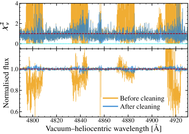
Figure 3: Example of manual cleaning of obvious artefacts and bad data from the spectrum of J014333$-$391700. Lower panel: The orange (light, background) spectrum is the result of the automatic phase of uves_popler and clearly shows the effect of bad CCD rows in the first 4 orders of red arm spectra (580-nm wavelength setting; not all contributing exposures were affected). The blue (dark, foreground) spectrum shows the result after the manual artefact removal stage in uves_popler: the most obvious artefacts were removed, but there are still some low-level effects from other contributing exposures that were not manually removed (e.g. at 4840, 4880 and 4920 Å). Upper panel: The $\chi^{2}$ spectra before (orange, background) and after (blue, foreground) artefact removal. $\chi^{2}$ for a given pixel is that of the contributing pixels’ flux values relative to their combined value (weighted mean). The $\chi^{2}$ spectra are used in uves_popler to help identify regions where artefacts may be present.

Another, less common, artefact in cpl-reduced UVES spectra is that of “bends”: echelle order spectra that have different shapes where they overlap. This can occur for several reasons, e.g. time-evolution in the flat-field lamp spectral shape, or poor extractions of the quasar flux near order edges, perhaps due to poorly constrained object traces. When very severe, these affected the final flux spectrum, and so were corrected. More subtle cases were still evident in the $\chi_{\nu}^{2}$ spectra and were corrected if they affected an obvious absorption line. Bends in contributing orders were corrected either by removing the bent section or by fitting a continuum to the order (or part thereof) and re-normalising it to match the combined spectrum’s continuum shape.

4.2.2 Order rescaling and combination

In spectral regions with very low S/N, or in echelle orders affected by severe artefacts, the relative scaling between an echelle order’s spectrum and the combined spectrum [step (v) in Section 4.1] can be very poorly or spuriously determined. This occurs frequently in the bluest orders of the 346 and 390-nm settings. It also occurs if the broad trough of a DLA straddles two echelle orders, and below the Lyman limit in the rest frame of DLAs and Lyman limit systems. In these latter examples, there is simply no flux to allow a relative scaling between adjacent orders; this is certainly a disadvantage of the order-scaling algorithm in uves_popler. To address this in DR1 spectra we manually adjusted the scaling of the highest-ranked order with an obvious scaling problem and re-ran the automatic scaling algorithm starting at that order. This process was repeated for lower-ranked orders to achieve a final spectrum that, visually, appears properly scaled. For the extreme blue orders, where the S/N degrades significantly, the best manual scaling factor to choose is often quite unclear, so there may be significant scaling differences between orders in regions of final spectra with $\textrm{S/N}\lesssim 5$ per pixel.

4.2.3 Continuum fitting

As discussed in Section 4.1, the continuum fit in uves_popler’s automatic phase is generally not useful in the $\textrm{Ly-}\alpha$ forest, near wide absorption features or over narrow emission lines. For the wide absorption and narrow emission features, we manually fit a new continuum only around the problematic region. This was relatively straight-forward, except for broad absorption-line quasars (BALs), because there are many pixels that are clearly not absorbed so the true continuum is easily discerned by the human eye. However, for the $\textrm{Ly-}\alpha$ forest, our approach was to manually fit the continuum in the entire region below the $\textrm{Ly-}\alpha$ emission line of all DR1 spectra. The well-known problem is that few $\textrm{Ly-}\alpha$ forest pixels are unabsorbed (except perhaps at redshifts $z\lesssim 2$), so the true continuum level is usually not at all clear. Our fitting approach is to manually select seemingly unabsorbed “peaks” in the $\textrm{Ly-}\alpha$ forest and interpolate between them with a low-order polynomial. This is done in chunks of spectrum ranging from $\sim$2000 to $\sim$50000 $\textrm{km\,s}^{-1}$ wide, depending on how variable the true continuum appears to be. The continuum fits to neighbouring chunks are blended together in a user-defined overlap region to ensure a smoothly-varying final continuum. In some chunks it is not possible to perform a polynomial fit in this way; for example, if BALs or DLAs fall near an emission line (most often the $\textrm{Ly-}\alpha$ emission line) the human eye can discern an approximate shape for a continuum fit but there clearly may be no pixels without substantial absorption to enable a fit. In these chunks, a continuum was simply drawn using a cubic spline function. Our $\textrm{Ly-}\alpha$ continuum fits are, therefore, necessarily subjective and uncertain; however, we expect that they are likely more accurate, and more predictably biased, than algorithmic approaches (certainly the ones currently available in uves_popler).

Figure 4 compares the automatic and manual continuum fits in part of the $\textrm{Ly-}\alpha$ forest in two $z_{\textrm{\scriptsize em}}\approx 3$ quasars. While the automatic continuum fit to the very high-S/N spectrum of J224708$-$601545 appears reasonable, on close inspection it is clearly too low in most regions and obviously too high around 4300 Å. However, for the lower-S/N spectrum of J013301$-$400628, the automatic continuum is completely inadequate. This is caused mainly by the emission line at 4160 Å. The manual fits shown in Figure 4 are clearly more accurate and useful for statistical studies of the $\textrm{Ly-}\alpha$ forest, and even for more detailed studies of these individual lines of sight. However, even by eye, one can identify potential problems with our manual fits. For example, the manual continuum redwards of $\sim$4300 Å in Figure 4 for J013301$-$400628 may by too high in general, perhaps by as much as $\sim$2%. We discuss the biases in our continuum fits in Section 5.2.1.

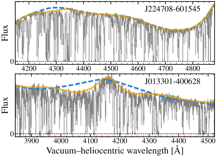
Figure 4: Example of automatic (blue dashed lines) and manual (orange solid lines) continuum fits in the $\textrm{Ly-}\alpha$ forest of two DR1 quasar spectra. For J224708$-$601545 (upper panel), the automatic and manual fits are very similar; in this case the parameters of the automatic continuum fitting algorithm of uves_popler were highly tuned to produce a reasonable fit, and this is aided by the very high S/N of the spectrum. For the lower-S/N spectrum of J013301$-$400628 (lower panel), no combination of fitting parameters could achieve a reasonable fit to the region shown here; the automatic fit shown reflects uves_popler’s default $\textrm{Ly-}\alpha$ forest fitting parameters: individual chunks of $\approx$250 Å are fit with a fourth-order polynomial. However, six separate manual continuum fits, in overlapping chunks, contributed to the final manual fit for the section of spectrum shown, with polynomial orders varying between 4 and 15; higher orders were needed to fit a reasonable continuum over the emission line at 4160 Å.

4.2.4 Quality control

All the authors, and several others (see Acknowledgements), contributed to the manual cleaning and continuum fitting steps outlined above. Of course, this may lead to varying quality and homogeneity among the final spectra. To reduce this, one author (MTM) reviewed all DR1 spectra and modified or added manual actions to improve and homogenise them, where necessary. While the purpose of the general cleaning steps above is to ensure a minimum quality and usefulness for all DR1 spectra, some spectra – or, most often, certain aspects of some spectra – have received much more extensive attention, including manual changes to the spectrum not described above. These are generally spectra that have already been published elsewhere. One example is the very detailed study of J051707$-$441055 to constrain cosmological variations in the fine-structure constant by Kotuš et al. (2017). Beyond the basic cleaning steps outlined above, this study focussed on correcting the individual exposures for known, long-range distortions of the UVES wavelength scale (e.g. Rahmani et al., 2013; Whitmore & Murphy, 2015) and velocity shifts between exposures caused by varying alignment of the quasar within the UVES slits. Such improvements are included in the DR1 versions of the spectra when available.

5 Database of final spectra

The final DR1 spectral database is available in Murphy et al. (2018). Each quasar’s final spectrum is provided in standard FITS format (Wells et al., 1981), with several FITS headers containing extensive information about the spectrum itself, the exposures that contributed to it and information about their extraction and calibration. We therefore expect that, for almost all scientific uses, only these final spectrum FITS files will be needed. However, for each quasar the database also contains the uves_popler log (UPL) file and cpl pipeline products from each contributing exposure. This allows any user to reproduce or modify the final spectrum using uves_popler. Furthermore, we also provide all the reduction scripts and lists of raw input science and calibration data; this allows the entire reduction procedure to be reproduced or modified if desired.

5.1 Basic spectral properties

Table 1 summarises information about the final spectra relevant for most scientific uses. These properties were determined as described below. We emphasise that the full observational information for every exposure is contained within the FITS header for each quasar (see documentation in Murphy et al., 2018).

5.1.1 Dispersion

The log-linear dispersion per pixel, expressed as a velocity in $\textrm{km\,s}^{-1}$, was chosen according to the on-chip binning used for the contributing exposures. The native pixel scale of UVES is $\approx$1.3 $\textrm{km\,s}^{-1}$ pix^-1 so this was the dispersion set for spectra for which most or all contributing exposures were unbinned in the spectral direction (i.e. 1$\times$1 binning). However, most quasars had all, or almost all, 2$\times$2 or 2$\times$1-binned (spectral $\times$ spatial) contributing exposures, so we set a 2.5 $\textrm{km\,s}^{-1}$ pix^-1 dispersion for these spectra. In more mixed cases we set intermediate dispersion values.

5.1.2 Wavelength coverage

Each quasar spectrum is accompanied by a pixel status spectrum whose integer value encodes whether each pixel is valid or the reason it is invalid. On a pixel-by-pixel basis, this array defines the detailed wavelength coverage map of the spectrum. However, for absorption-line searches, a more useful definition ignores single invalid pixels within larger, contiguous valid regions. Each DR1 FITS header therefore includes a wavelength coverage map in which valid chunks must be at least 100 $\textrm{km\,s}^{-1}$ wide and contain gaps (runs of invalid pixels) no wider than 10 $\textrm{km\,s}^{-1}$. Table 1 shows an abridged version of this wavelength coverage map.

The upper panel of Figure 5 illustrates the total wavelength coverage of all 467 DR1 quasars with final spectra. The many detailed features in this map generally reflect the different wavelength settings used in the UVES observations. For example, the broad bump at $\sim$3800 Å is where the 390 and 437 nm settings overlap, while the dip at $\sim$4500 Å is where the 390-nm wavelength coverage ends and where that of the 564-nm setting begins. The series of narrow dips redwards of $\sim$9500 Å are due to gaps in wavelength coverage between neighbouring echelle orders (i.e. where the free spectral range exceeds the CCD width). The lower panel of Figure 5 shows the total wavelength coverage in the common quasar rest frame. Here the focus on rest wavelengths $\lesssim$2800 Å is evident, which is driven by the relative lack of strong absorption lines redwards of the Mg ii doublet ($\lambda\lambda$2796/2803).

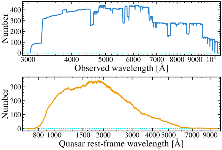
Figure 5: Total wavelength coverage of the 467 final DR1 quasar spectra in the observed frame (upper panel) and common quasar rest frame (lower panel). The wavelength coverage of an individual spectrum is determined by requiring that valid chunks (contiguous runs of valid pixels) must be at least 100 $\textrm{km\,s}^{-1}$ wide and contain gaps (runs of invalid pixels) no wider than 10 $\textrm{km\,s}^{-1}$.

5.1.3 Continuum-to-noise ratio (C/N)

Each DR1 FITS header provides the median C/N of the spectrum in bins of 1000 $\textrm{km\,s}^{-1}$. Table 1 presents these C/N values for the bins with wavelength centres closest to 3500, 4500, 5500, 6500 and 7500 Å. The left panel of Figure 6 shows the C/N distribution for the DR1 quasars at these wavelengths. Here, for uniform treatment of quasars with different dispersions, the C/N in has been converted a per-2.5-$\textrm{km\,s}^{-1}$-pixel value for all quasars. Most DR1 quasar spectra have C/N in the range 5–60. However, a substantial number of spectra (26 at 5500 Å and 28 at 6500 Å) have $\textrm{C/N}>100$ per 2.5-$\textrm{km\,s}^{-1}$ pixel. Of course, the C/N in the most sensitive region of the spectrograph ($\sim$5500–6500) has a non-zero minimum, but the minimum extends to essentially zero for the bluer regions, particularly at wavelengths $\sim$3500 Å. The right panel of Figure 6 shows the C/N distributions at five wavelengths in the common quasar rest-frame which characterise the data quality in the $\textrm{Ly-}\alpha$ forest near the Lyman limit (935 Å) and $\textrm{Ly-}\alpha$ emission line (1170 Å), and in three regions redwards of $\textrm{Ly-}\alpha$ – 1450, 1690, 2200 Å – which are known to be relatively free of quasar emission lines (e.g. Vanden Berk et al., 2001; Murphy & Bernet, 2016)

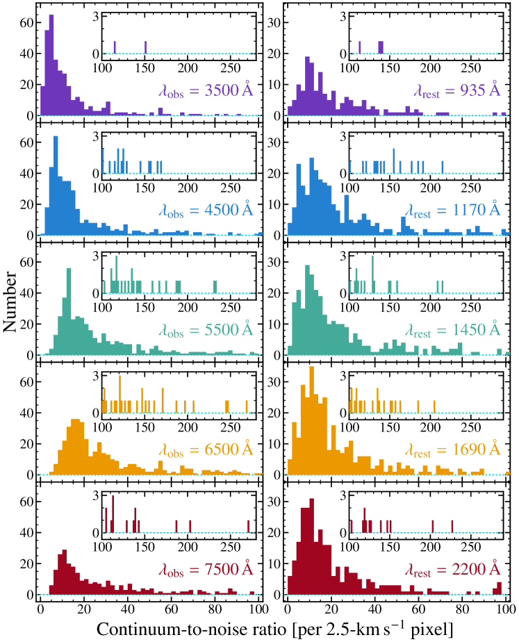
Figure 6: Distribution of continuum-to-noise ratio (C/N) per 2.5-$\textrm{km\,s}^{-1}$ pixel for the 467 DR1 quasars with final spectra. The left panel shows the C/N distributions at a series of representative observed wavelengths. The right panel shows the C/N distributions in the common quasar rest frame at two representative $\textrm{Ly-}\alpha$ forest wavelengths (935 and 1170 Å) and three relatively emission-line free wavelengths redwards of $\textrm{Ly-}\alpha$. The C/N is measured as the median value within a 1000-$\textrm{km\,s}^{-1}$ window around the nominated wavelength. The inset in each panel shows the high-C/N tail of each distribution. Note that a small number of spectra have even higher C/N at some wavelengths than the insets cover. For example, J051707$-$441055 has $\textrm{C/N}=342$ per 2.5-$\textrm{km\,s}^{-1}$ pixel at 5500 Å, the highest in the DR1 sample.

5.1.4 Nominal resolving power ($R_{\rm nom}$)

$R_{\rm nom}$ is the mean resolving power of the contributing exposures, in 1000 $\textrm{km\,s}^{-1}$-wide bins, determined from their slit widths, assuming the slit is uniformly illuminated. For quasar exposures where the seeing was similar to, or smaller than, the slit width, the real resolving power will be somewhat higher than the nominal value; for example, Kotuš et al. (2017) found that an $\approx$10% increase in resolving power is typically expected. Each DR1 FITS header provides $R_{\rm nom}$ for all bins (within the wavelength coverage of the spectrum), while Table 1 includes values only for the bins with wavelength centres closest to 3500, 4500, 5500, 6500 and 7500 Å. $R_{\rm nom}$ was modelled as a second-order polynomial of slit width, $d_{\rm slit}$, in arcseconds: $R_{\rm nom}=a_{0}+a_{1}d_{\rm slit}+a_{2}d_{\rm slit}^{2}$. The polynomial coefficients, $a_{i}$, shown in Table 2 were derived by fitting the resolving power against slit width of the ThAr exposures in ESO’s UVES quality control database for years 2010–2016. Seperate sets of coefficients were derived for the blue arm (from the 390-nm setting) and red arm (580-nm setting), and for unbinned and 2$\times$2-binned ThAr exposures (with 0.4–1.2 and 0.8–1.4 arcsecond slit widths, respectively). The two CCD chips in the red arm were found to have very similar resolving powers in all cases, so they have been treated together and assigned the same coefficients. Some or all of the contributing exposures to 11 DR1 quasars were binned 3$\times$2; however, their nominal resolving powers were assumed to be the same as for 2$\times$2-binned exposures.

Table 2: Polynomial coefficients used to determine the nominal resolving power (i.e. for a uniformly illuminated slit), as a function of slit width: $R_{\rm nom}=a_{0}+a_{1}d_{\rm slit}+a_{2}d_{\rm slit}^{2}$ for $d_{\rm slit}$ in arcseconds. See text in Section 5 for details.

Arm	Binning	$a_{0}$	$a_{1}$	$a_{2}$
Blue	None	10033	63237	$-$24986
Blue	2$\times$2	22011	50563	$-$22803
Red	None	8533.3	52709	$-$16005
Red	2$\times$2	28846	28505	$-$9533.3

5.2 Remaining artefacts, systematic effects and limitations

While we invested significant effort to ensure that at least a minimum standard of cleaning and quality control was applied to each spectrum (see Section 4.2), there are numerous remaining artefacts in all DR1 spectra. We discuss the most prominent of these below. It is important that users of the DR1 spectra consider the effect these remaining artefacts may have on their analyses; we expect that most statistical analyses of the spectra will be somewhat sensitive to one or more of these artefacts. Users are encouraged to discuss these and other potential (or more subtle) systematic effects with the corresponding author (MTM).

5.2.1 Continuum errors

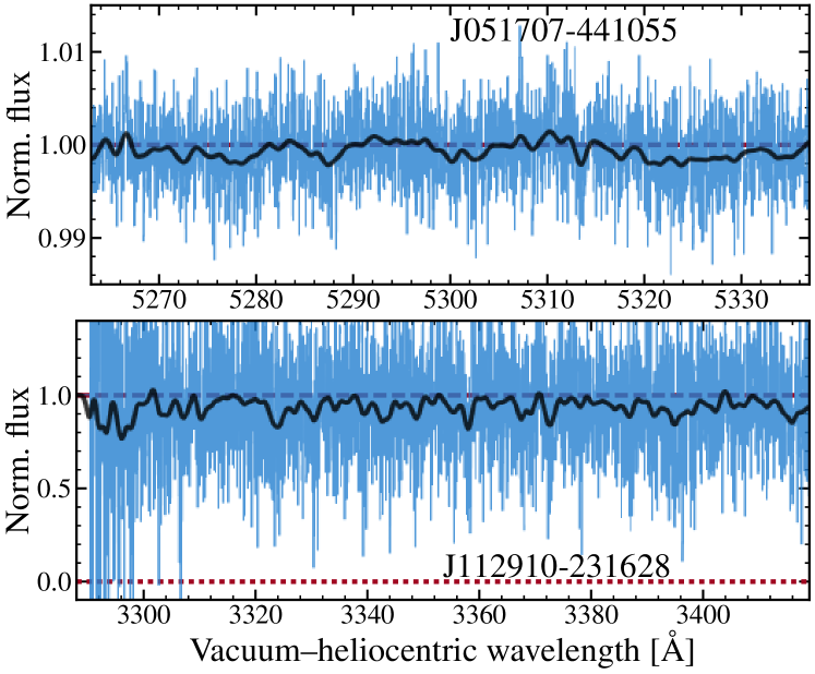
Figure 7: Examples of overestimated automatic continuum level (redwards of the $\textrm{Ly-}\alpha$ emission line). The top panel shows a very high S/N region while the bottom panel shows a very low S/N region, i.e. the extreme blue end of the 390-nm standard wavelength setting. The spectra (blue/grey) have been smoothed (black) by a Gaussian filter (with a 20-pixel kernel) to aid the eye in discerning the bias in the continuum level. In both cases, the continuum is generally overestimated by up to $\sim$0.25 times the flux RMS. That is, the magnitude of the bias scales with the S/N; analyses of lower-S/N DR1 spectra are more likely to be affected by this bias.

As discussed in Section 4.1 and Section 4.2.3, the continuum in most regions redwards of the $\textrm{Ly-}\alpha$ emission line is automatically fit, while it is manually fit in the $\textrm{Ly-}\alpha$ forest. In addition to the inherent inaccuracy in defining a $\textrm{Ly-}\alpha$ forest continuum (see Section 4.2.3), these two approaches cause two significant systematic continuum errors in the DR1 spectra:

1. Overestimated automatic continuum fit: Even in (by-eye) completely unabsorbed regions redwards of the $\textrm{Ly-}\alpha$ emission line, the automatic continuum level is generally slightly overestimated. The mean continuum-normalised flux in such regions lies 0.05–0.25$\bar{\sigma}$ below unity, for $\bar{\sigma}$ the mean normalised flux uncertainty. This continuum overestimate is caused by the asymmetric prejudice built in to our iterative continuum fitting algorithm (see Section 4.1): absorption features are far more common than (spurious) emission features (e.g. cosmic rays), so the algorithm rejects pixels with flux (default values) $>$3.0$\sigma$ above and $>$1.4$\sigma$ below the current fit for the next iteration. For high S/N DR1 spectra, this effect is clearly a small fraction of the continuum level and therefore unlikely to cause problems for most analyses. The upper panel of Figure 7 shows an example. However, the overestimate will be a larger proportion of the continuum level for lower-S/N regions of all DR1 spectra; for example, the lower S/N at the blue extreme of many spectra causes a noticeable overestimate, as illustrated in the lower panel of Figure 7.

2. Redshift-dependent bias in manual continuum fits of the $\textrm{Ly-}\alpha$ forest: As described in Section 4.2.3, our approach to manually fitting a continuum in the $\textrm{Ly-}\alpha$ forest involved visually identifying “seemingly unabsorbed peaks” and interpolating between them with the same iterative polynomial fitting algorithm used redwards of the $\textrm{Ly-}\alpha$ emission line. Upon very close inspection of the DR1 spectra, there appear to be convincingly unabsorbed continuum regions of the $\textrm{Ly-}\alpha$ forest at $z\lesssim 3$; i.e. the lower number density of forest lines leaves more truly unabsorbed regions to fit. Therefore, we expect at least the same overestimation of the continuum in the $z\lesssim 3$ $\textrm{Ly-}\alpha$ forest as described in point (i) above. However, the increasing $\textrm{Ly-}\alpha$ forest line density means that few (or no) truly unabsorbed regions exist at higher redshifts, so our fits will underestimate the true continuum. While it is likely to increase with redshift, it is difficult to estimate the magnitude of this bias. However, we refer users of DR1 spectra to the study by Becker et al. (2007) as a guide: using a similar continuum fitting approach, fitting theoretical models of the $\textrm{Ly-}\alpha$ flux probability distribution required upward adjustments to their continuum levels by $\lesssim$3% at $z\sim 3$, and by $\sim$7–17% at $z\sim 4$–5.

Finally, the incidence of Lyman-limit systems (where there is significant remaining flux bluewards of the limit) and broad absorption line (BAL) features makes the definition of the continuum dependent on the scientific question being addressed: for example, what constitutes the continuum is very different when studying a Lyman limit or the $\textrm{Ly-}\alpha$ forest bluewards of it. Generally, in such cases, we attempted to fit or interpolate a continuum that would be useful for most users. However, we urge those studying Lyman-limit systems and BALs in DR1 spectra to redefine the continuum placement accordingly.

5.2.2 Telluric features

Figure 8 illustrates the strongest common telluric features in the DR1 spectra. In general, no attempt was made to remove telluric features in individual spectra. While, in principle, variation of the heliocentric velocity among a large number of exposures, plus our iterative removal of outlying data when combining exposures, can remove many telluric features from the final spectrum, these criteria are rarely met in practice. This means that most DR1 spectra contain many telluric absorption lines – particularly the O₂ $\gamma$, B and A bands ($\sim$6300, 6880 and 7620 Å, respectively) and the H₂O bands at $\approx$6470–6600, 6830–7450, 7820–8620 and 8780–10000 Å – and residuals from imperfectly subtracted sky emission lines, particularly at $\gtrsim$7000 Å, the strong O i $\lambda$5578 sky emission line and the Na i $\lambda$5891/5897 doublet. In the few spectra with high S/N at $\lesssim$3400 Å, the broad Huggins ozone bands are visible. If these bands occurred redwards of the $\textrm{Ly-}\alpha$ forest (i.e. for quasars at $z_{\textrm{\scriptsize em}}\lesssim 1.5$), they were reasonably well fit by our continuum-fitting process, but our fits are not likely to reflect the complex shapes of individual bands. However, for higher redshift quasars, our continuum fitting approach generally ignored the Huggins bands; users of such spectra should be cautious of the continuum fit and corresponding normalised flux spectrum below $\approx$3300 Å.

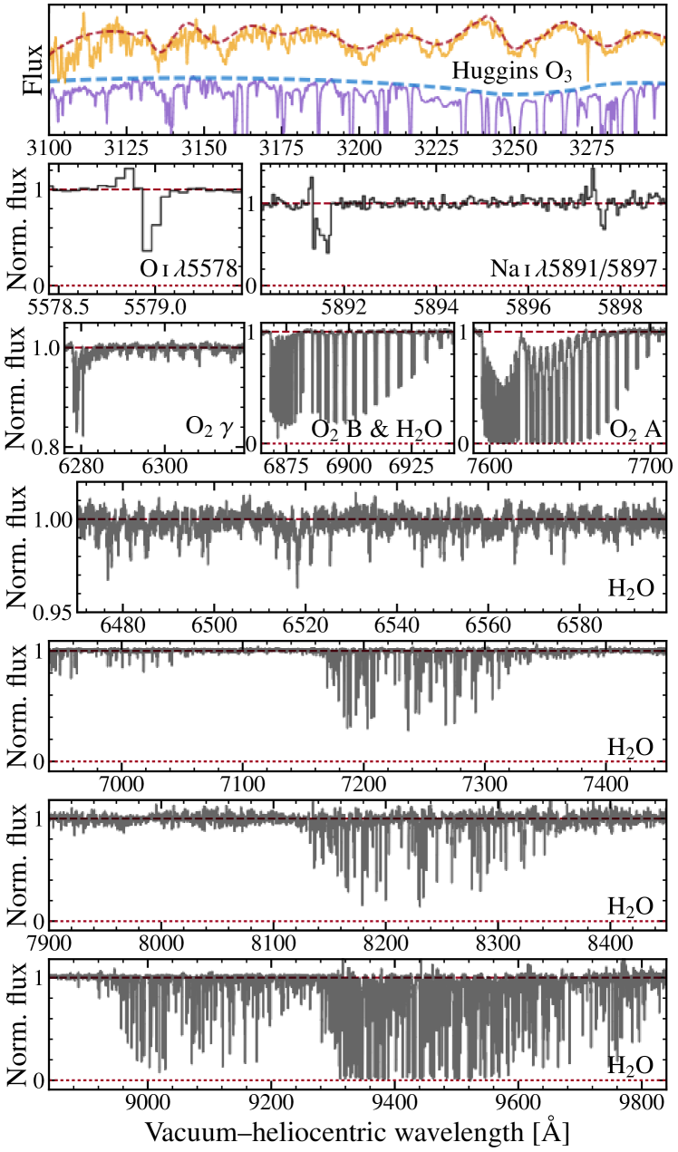
Figure 8: Common, strong telluric features in the DR1 quasar spectra. The top panel shows two spectra (J051707$-$441055: lower, purple; J083052$+$241059: upper, orange; both are Gaussian-smoothed with a 6-pixel kernel for clarity) affected by the broad Huggins O₃ bands at $\lesssim$3300 Å. This is easily seen in the upper spectrum which does not cover the $\textrm{Ly-}\alpha$ forest: our undulating continuum fit (dashed line) largely matches the band shapes (though not completely; e.g. the broad dips below the continuum fit near $\approx$3156, 3202 and 3225 Å). These bands are not fitted in the lower spectrum because it covers the $\textrm{Ly-}\alpha$ forest. The second row of panels show poorly subtracted telluric emission lines: O i $\lambda$5578 in J124913$-$055919 and Na i $\lambda$5891/5897 in J001306$+$000431). The other panels show strong molecular absorption bands in J051707$-$441055.

5.2.3 Cosmic rays and bad pixels

The cpl data reduction suite, and the post-reduction processing and combination of exposures in uves_popler, both attempt to identify and mask ‘cosmic rays’ and bad pixels. However, many remain unidentified and, at least, imperfectly removed from individual exposures. DR1 spectra with fewer contributing exposures therefore contain many, generally narrow ($\lesssim$5 pixels wide) remaining cosmic rays and bad pixel residuals. These are much less common in spectra with more than $\sim$5 contributing exposures. Nevertheless, even in such cases, users should be cautious of residual cosmic ray and bad pixel artefacts in deep absorption lines: as Figure 9 illustrates uves_popler does not remove sharp, positive flux spikes in regions of low local relative flux because these can be real velocity structure in metal-line absorption systems. These were generally not removed in our manual cleaning process.

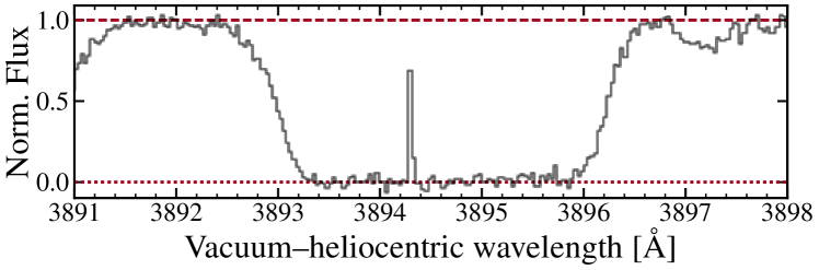
Figure 9: Example of a ‘cosmic ray’ (at 3894.2 Å) in the saturated core of $\textrm{Ly-}\alpha$ forest line in the DR1 spectrum of J033108$-$252443. uves_popler does not remove such artefacts because similar, real spectral features are often seen in saturated metal lines, and our manual cleaning process did not attempt to identify and remove all such artefacts.

5.2.4 Unidentified absorption artefacts

During the manual cleaning process, several features were noticed in many spectra that, in some cases, were clearly not due to real absorption systems: they had slightly different positions and shapes in different exposures of the same quasar, similar to the artefacts from bad rows of CCD pixels discussed in Section 4.2.1, but much narrower and weaker in general. When these features were clearly spurious they were manually removed. However, in many spectra, the author cleaning the spectrum either did not notice these artefacts – they vary in strength considerably from quasar to quasar, and can be weak (or apparently absent) and not obvious to visual inspection – or there was not enough evidence to confirm they were not real absorption lines (e.g. there was not a significant difference between the features in different exposures). Upon completion of the cleaning of all DR1 spectra, it was clear that similar features were often found at similar wavelengths in different quasar spectra, confirming their spurious origin. However, their origin is not currently clear. Simple checks for bad pixel runs, ThAr remnants and flat-field features did not reveal a clear cause.

To more systematically reveal these unidentified features, and other common remaining artefacts, we combined the final spectra of the 131 DR1 quasars at $z<1.5$. The redshift criterion ensures that the composite is not contaminated by the $\textrm{Ly-}\alpha$ forest. The spectra were redispersed onto a common vacuum–heliocentric wavelength scale with 2.5-$\textrm{km\,s}^{-1}$ per pixel dispersion and combined using a clipped mean for each pixel. A contributing pixel with flux more than 3$\sigma$ below, or 4$\sigma$ above, the mean was removed ($\sigma$ is its flux uncertainty) to avoid real absorption lines or sky-line emission residuals and reveal features common to many spectra.

Figure 10 shows the main unidentified artefacts revealed by the composite spectrum at 4716, 4744, 5240, and 5580–5800 Å. The width and shape of the composite features reflects those found in individual spectra. However, they do seem to appear at slightly different (vacuum–heliocentric) wavelengths in individual spectra, so the composite features may be somewhat broadened. The composite spectrum also reveals many weaker features. We provide the clipped mean composite DR1 spectrum in Murphy et al. (2018) so that users can utilise it directly to identify and mask spurious spectral features that may affect their absorption line surveys.

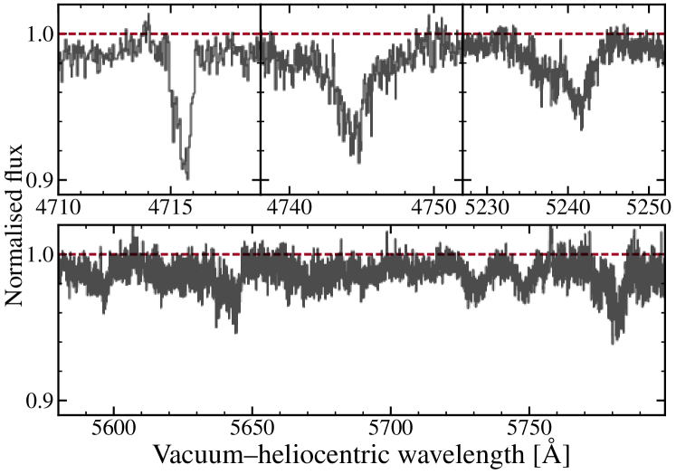
Figure 10: Main unidentified artefacts revealed by the clipped mean composite spectrum of $z_{\textrm{\scriptsize em}}<1.5$ DR1 quasars. These features are detectable in many, but certainly not all, individual DR1 spectra. In some cases they were removed in the manual cleaning process, but not in most cases, as the composite spectrum shows.

5.2.5 Underestimated uncertainties at low flux levels

Common to all DR1 spectra is that the flux uncertainty arrays of individual cpl-reduced exposures are underestimated when the quasar flux is low. This is easily noticed in uves_popler as peaks in the $\chi^{2}_{\nu}$ spectrum (see Section 4.2.1) in strong and, especially, saturated absorption lines, or where the S/N of individual exposures is $\lesssim$5 per pixel. It is therefore most noticeable in the $\textrm{Ly-}\alpha$ forest. Figure 11 illustrates two examples in the $\textrm{Ly-}\alpha$ forest of one DR1 quasar spectrum. $\chi^{2}_{\nu}$ typically reaches $\sim$2 in such regions, indicating that the uncertainty array is underestimated by a factor of $\sim$1.4. However, this factor depends on the S/N of individual exposures: it tends to be larger for lower S/N exposures. We suspect that the cpl reduction pipeline underestimates the noise contribution from the sky flux during the optimal extraction. This problem also existed in the previous, eso-midas data reduction code for UVES. To compensate some of its effects on absorption line studies, some authors have increased the flux uncertainty estimate in the cores of deep/saturated absorption lines in UVES spectra (e.g. King et al., 2012).

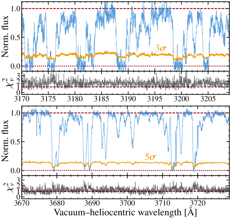
Figure 11: Example of the underestimated uncertainty spectrum in regions of low flux. Top two panels: Final DR1 spectrum (blue, dark) of J033108$-$252443 in a region where all 14 contributing exposures have low S/N ($\lesssim$5 per pixel) and, therefore, where the uncertainty spectrum (orange, light; shown as 3$\sigma$ for clarity) is dominated by sky photon noise; this is also indicated by its low contrast between areas of unabsorbed continuum and saturated lines. The corresponding $\chi^{2}_{\nu}$ spectrum ($\chi^{2}$ per degree of freedom of the flux in the contributing exposures around the weighted mean flux) is generally higher than expected – i.e. $\approx$2 (c.f. expectation of $\approx$1) – demonstrating that the uncertainty spectrum is underestimated. Lower two panels: Same as upper two panels but for a higher S/N region. Here, the quasar photon noise dominates and $\chi^{2}_{\nu}$ is $\approx$1 in unabsorbed regions. However, in strong or saturated lines, where the sky photon noise dominates, $\chi^{2}_{\nu}$ increases to $\approx$2. This indicates that the sky noise contribution is underestimated.

5.2.6 Bad data in individual exposures

As noted in Section 4.2.1, our approach for removing bad data from contributing exposures was to do so when they affected an obvious absorption feature. Artefacts from remaining bad data may still affect, or even mask, very weak absorption features that were not noticed by eye in the manual cleaning process. Users aiming to detect weak absorption features in the individual DR1 spectra are advised to inspect the flux, uncertainty and $\chi^{2}_{\nu}$ spectra – of both the combined spectra and their contributing exposures – in detail. Indeed, uves_popler was specifically designed to display these details to allow such specific quality control steps.

5.2.7 Blaze function variations and remnants

The blaze function for each echelle order of an exposure is approximated using the master flat field by the cpl reduction software. This, in principle, can change from exposure to exposure as the alignment of optical elements change slightly with time or wavelength setting, or with changes in the flat field lamp spectrum (e.g. as it ages) or illumination pattern on the CCDs. As explained in Section 4.2.1, these effects (and possibly others) cause “bends” between the spectral shapes of spectra from overlapping orders, the most obvious of which we attempted to identify and correct in the manual cleaning process. Our priority was to address this problem when it affected an obvious absorption line. However, for very weak absorption features (especially broader ones) that may not have been noticed by eye, weak bends may not have been removed. And, where obvious absorption lines were not found, noticeable bends will still be present in the DR1 spectra, particularly in high S/N cases. An example of remaining bends in the spectrum of the bright quasar J133335$+$164903 is shown in the upper panels of Figure 12.

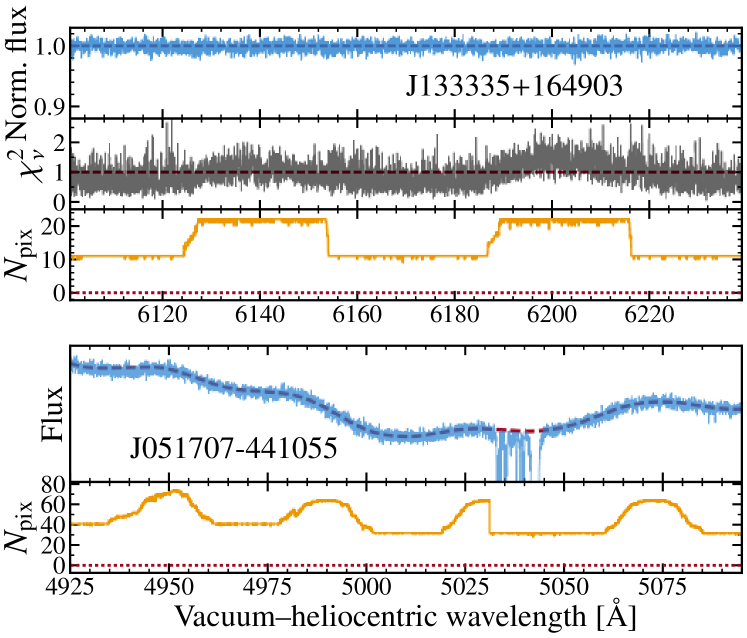
Figure 12: Examples of artefacts remaining from the blaze function removal. Top panels: Spectra from overlapping echelle orders may have different shapes in the overlap region – “bends” – causing higher $\chi^{2}_{\nu}$ values and, potentially, spurious effects on weak absorption features in the combined spectrum. The $N_{\rm pix}$ spectrum shows the number of contributing echelle orders. The increase from $N_{\rm pix}\approx 11$ to $\approx$22 indicates the overlap region of neighbouring echelle orders; the increase in $\chi^{2}_{\nu}$ in these overlap regions is due to bends. In this example, no adverse effects on the normalised flux spectrum are apparent. Lower panels: Imperfect blaze function removal leaves broad undulations in the flux spectrum that coincide with the overlap region between echelle orders (indicated by the $N_{\rm pix}$ spectrum). In this example, note the sharp drop in the $N_{\rm pix}$ spectrum at $\approx$5031 Å: the low-S/N red ends of the echelle orders covering $\approx$4990–5040 Å have been manually removed to ensure they did not affect the strong absorption line system at $\approx$5031–5045 Å.

The correction for the blaze function also appears to be imperfect in systematic ways. Many DR1 spectra therefore contain remnants of the blaze function that appear as ripples or undulations in the flux spectrum over echelle-order scales. An example is shown in the lower panels of Figure 12. These undulations have amplitudes $\lesssim$5% of the continuum level, and are usually substantially smaller. In non-$\textrm{Ly-}\alpha$ forest regions, our continuum fitting approach will largely correct for these blaze remnants, as is evident in Figure 12. However, in $\textrm{Ly-}\alpha$ forest regions, where individual continuum fits cover a larger range of wavelengths, and where the forest obscures such broad, shallow undulations, these blaze remnants may still significantly affect the final normalised flux spectrum.

5.2.8 Zero level errors

Inspection of cpl-extracted UVES exposures with relatively low S/N often reveals imperfect zero levels: the average flux in saturated line cores is significantly different to zero. This indicates that the sky flux level is inaccurately measured in the optimal extraction process. Figure 13 shows some typical examples of this problem in DLA absorption troughs (upper panel) and saturated $\textrm{Ly-}\alpha$ forest line cores (lower two panels). As the figure illustrates, the zero-level error in some final spectra can be of order $\sim$2–4%; in extreme cases – exposures with very low S/N, where the trace of the quasar is not well determined – the error can be up to $\sim$10%. Figure 13 also shows that the zero level can be overestimated or underestimated (compare the lower two panels) and that, in some cases, it can vary from too low to too high over relatively short wavelength ranges (upper panel); however, in most cases the zero level error appears to have the same sign and not vary substantially in magnitude over much larger wavelength ranges (typically $\gtrsim$300 Å). We have not attempted to correct for these zero-level errors in the DR1 spectra so users should account for them when, for example, modelling strong or saturated absorption lines (e.g. DLAs).

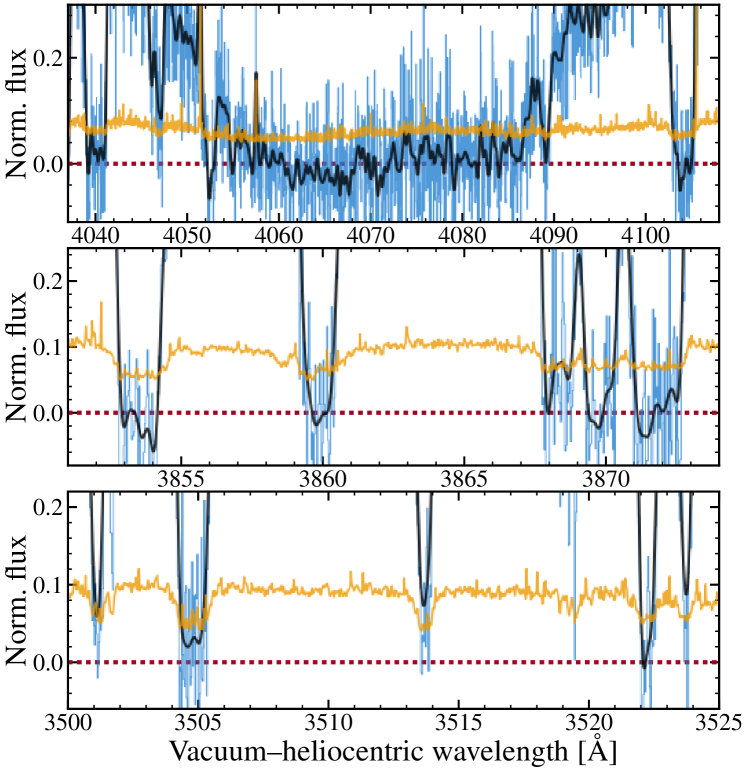
Figure 13: Examples of zero-level errors in the DR1 spectra. The spectra (blue histograms) have been smoothed (black line) to show a running average flux, compared with the 1$\sigma$ uncertainty array (light, orange line). Top panel: A DLA trough in the spectrum of J020900$-$455026 where the zero level varies from $\approx$3% too high ($\approx$4061–4068 Å) to $\approx$2% too low ($\approx$4072–4084 Å) over a relatively short wavelength range. Middle panel: Saturated $\textrm{Ly-}\alpha$ forest line cores where the zero level is overestimated by $\approx$1–3% (same spectrum as top panel). Bottom panel: Saturated $\textrm{Ly-}\alpha$ forest lines in the spectrum of J231359$-$370446 where the zero level is underestimated by $\approx$2–3%.

5.2.9 Wavelength scale shifts and distortions

The wavelength calibration accuracy of UVES has been the specific focus of many quasar absorption studies, particularly those seeking to constrain possible variations in the electromagnetic fine-structure constant and proton-to-electron mass ratio (using metal-line and H₂ absorption, respectively). The wavelength scale is set by comparison with a ThAr lamp exposure, and several effects shift and/or distort the true quasar wavelength scale with respect to this:

1. Mechanical drifts and changes in the refractive index of air were designed to be compensated for by resetting the grating angles (Dekker et al., 2000) which, in practice, is limited to $\sim$0.1–0.2 $\textrm{km\,s}^{-1}$ accuracy;

2. Differences in alignment of the quasar in a slit between exposures, and/or between the two slits (i.e. between the spectrograph arms), produces (approximately) velocity-space shifts of, typically, up to $\sim$0.4 $\textrm{km\,s}^{-1}$ (e.g. Molaro et al., 2013; Rahmani et al., 2013; Evans et al., 2014; Kotuš et al., 2017) and up to $\sim$2 $\textrm{km\,s}^{-1}$ in extreme cases;

3. Intra-order distortions (i.e. wavelength-dependent shifts on echelle order scales), that have a largely (but not entirely) repeated shape and amplitude from order to order, have amplitudes of typically $\sim$0.1 $\textrm{km\,s}^{-1}$ (up to 0.4 $\textrm{km\,s}^{-1}$ in extreme cases; e.g. Whitmore et al., 2010; Whitmore & Murphy, 2015);

4. Long-range distortions between the science object and ThAr wavelength scales have been identified that have magnitudes of typically $\sim$0.1 $\textrm{km\,s}^{-1}$ per 1000 Å and up to $\sim$4 times larger in extreme cases (e.g. Rahmani et al., 2013; Bagdonaite et al., 2014; Whitmore & Murphy, 2015).

The magnitude, sign and shape of the latter two distortion effects is quite variable, and can change substantially over $\sim$1–3 day periods.

In general, the individual exposures and final DR1 spectra are not corrected for the above effects. However, they are relatively small – typically $\lesssim$20 % of a (unbinned) pixel – so are not likely to significantly affect most applications. A small number of DR1 spectra have been corrected using asteroid or iodine-cell stellar observations (e.g. Evans et al., 2014), solar twin stars (e.g. Daprà et al., 2015, 2016) or spectra of the same object on better-calibrated spectrographs (e.g. Kotuš et al., 2017). The UPL files include these corrections in such cases.

6 Scientific uses

As described in Section 1, numerous scientific questions can be addressed with the DR1 quasar spectra. In this section we seek to highlight and assist the large-scale statistical studies of quasar absorption systems that are possible with such a large sample of high-resolution spectra. Specifically, we illustrate how the DR1 spectra will be useful for detailed DLA studies, absorption line surveys, and studies of time-variable absorption lines.

6.1 Damped $\textrm{Ly-}\alpha$ system studies

DLAs contain most of the neutral hydrogen in the universe at all epochs currently probed, from $z\sim 5$ down to 0 (see review by Wolfe et al., 2005). Their high H i column densities – $N_{\textsc{h\scriptsize{\,i}}}\geq 2\times 10^{20}$ $\textrm{cm}^{-2}$, by definition – shield the gas from ionising radiation, allowing it to remain highly neutral, presumably making DLA gas available for later star formation. DLAs also contain a large proportion of the universe’s metals; studying their chemical abundances and metallicities – and how these evolve with redshift – are therefore important elements in understanding galaxy formation and evolution. DLA metal abundances and metallicities can be very accurately measured, owing to the simple relationship between optical depth and column density, and the neutrality of the DLA gas (i.e. no corrections for ionised hydrogen or metals are generally required). The most accurate and precise DLA metal-line measurements are possible in high-resolution spectra because the metal line velocity structures can be resolved.

For these reasons, the DR1 quasar spectra offer an excellent opportunity for detailed studies of a large sample of DLAs. To assist such work, we have identified 155 DLAs towards the 467 DR1 quasars with final spectra and catalogued them in Table 3. While 137 of the DLAs in Table 3 have previously been reported in the literature, the other 18 are reported here for the first time (to our knowledge).

Table 3: The DR1 sample of 155 DLAs. 132 DR1 quasar spectra have previously reported DLAs (i.e. $N_{\textsc{h\scriptsize{\,i}}}\geq 2\times 10^{20}$ $\textrm{cm}^{-2}$; references 1–22 in the final column) where the $\textrm{Ly-}\alpha$ transition is detected in the DR1 spectrum. 18 new DLAs are reported below (reference 23 in the final column) for which we have measured $N_{\textsc{h\scriptsize{\,i}}}$ from the DR1 spectra.

DR1 Name	$z_{\rm em,Adopt}$	$z_{\textrm{\scriptsize abs}}$	$\log(N_{\textsc{h\scriptsize{\,i}}}/\textrm{cm}^{-2})$	$\sigma(\log N_{\textsc{h\scriptsize{\,i}}})$	Ref.a
J000149$-$015939	2.815	2.095	20.65	0.10	20
J000149$-$015939	2.815	2.154	20.3	0.1	20
J000443$-$555044	2.100	1.886	20.4	0.1	23
J000651$-$620803	4.455	2.970	20.7	0.2	20
J000651$-$620803	4.455	3.202	20.8	0.1	20
J000815$-$095854	1.955	1.768	20.85	0.15	20
J001306$+$000431	2.164	2.025	20.95	0.10	20
J001602$-$001225	2.085	1.973	20.83	0.05	20
J003023$-$181956	2.550	2.402	21.75	0.10	20
J004054$-$091526	4.976	4.740	20.39	0.11	20
J004131$-$493611	3.240	2.248	20.46	0.13	20
J004216$-$333754	2.480	2.224	20.6	0.1	20
J004435$-$262259	2.980	2.549	21.5	0.2	23
J004508$-$291432	2.388	1.809	20.4	0.1	20
J004508$-$291432	2.388	1.936	20.5	0.1	20
J005127$-$280433	2.256	2.071	20.45	0.10	12
J010104$-$285801	3.070	2.671	21.1	0.1	20
J010311$+$131617	2.705	2.309	21.35	0.08	20
J010516$-$184642	3.025	2.370	21.00	0.08	20
J011453$+$031457	2.810	2.423	20.90	0.10	10
J011504$-$302514	2.985	2.418	20.50	0.08	20
J011504$-$302514	2.985	2.702	20.3	0.1	20
J012517$-$001828	2.274	1.761	20.78	0.07	20
J012550$-$535225	3.180	2.837	21.2	0.1	23
J013340$+$040059	4.172	3.692	20.68	0.15	20
J013340$+$040059	4.172	3.773	20.42	0.10	20
J013754$-$270736	3.210	2.107	20.30	0.15	10
J013754$-$270736	3.210	2.800	21.00	0.10	10
J013901$-$082444	3.013	2.677	20.70	0.15	20
J014049$-$083942	3.713	3.696	20.75	0.15	17
J014214$+$002324	3.370	3.348	20.38	0.05	17
J020900$-$455026	2.520	2.349	21.0	0.1	23
J020944$+$051713	4.184	3.666	20.47	0.10	20
J020944$+$051713	4.184	3.863	20.43	0.15	20
J021741$-$370059	2.910	2.429	20.62	0.08	20
J021741$-$370059	2.910	2.514	20.46	0.09	20
J021857$+$081727	2.991	2.293	20.45	0.16	20
J024449$-$290449	3.230	2.560	20.8	0.2	23
J025240$-$553832	2.370	2.340	20.6	0.1	23
J025634$-$401300	2.290	2.046	20.45	0.08	20
J030211$-$314030	2.370	2.179	20.8	0.1	12
J030722$-$494548	4.728	4.466	20.67	0.09	4
J032412$-$320259	3.302	2.243	20.5	0.1	23
J033025$-$495403	2.230	1.893	21.2	0.2	23
J033413$-$161205	4.363	3.557	21.12	0.15	8
J033854$-$000521	3.050	2.230	21.05	0.25	20
J033900$-$013317	3.197	3.062	21.20	0.09	20
J034943$-$381030	3.205	3.025	20.73	0.05	20
J040718$-$441013	3.000	1.913	20.8	0.1	20
J040718$-$441013	3.000	2.551	21.15	0.15	20
J040718$-$441013	3.000	2.595	21.05	0.10	20
J040718$-$441013	3.000	2.621	20.45	0.10	20
J041656$-$284340	2.090	1.719	21.2	0.2	23
J042353$-$261801	2.277	2.157	20.65	0.10	12
J042644$-$520819	2.250	2.224	20.3	0.1	12
J043255$-$355030	2.280	1.961	20.7	0.1	23
J043403$-$435547	2.649	2.302	20.78	0.10	20
J044017$-$433308	2.863	2.347	20.78	0.12	20
J044534$-$354704	2.610	2.408	20.3	0.1	23
J045313$-$130555	2.300	2.067	20.50	0.07	20

Table 4: continued

$\!\!.$ The DR1 sample of 155 DLAs.

DR1 Name	$z_{\rm em,Adopt}$	$z_{\textrm{\scriptsize abs}}$	$\log(N_{\textsc{h\scriptsize{\,i}}}/\textrm{cm}^{-2})$	$\sigma(\log N_{\textsc{h\scriptsize{\,i}}})$	Ref.
J050112$-$015914	2.286	2.040	21.7	0.1	20
J053007$-$250329	2.813	2.141	20.95	0.05	20
J053007$-$250329	2.813	2.811	21.35	0.07	20
J055246$-$363727	2.317	1.962	20.70	0.08	20
J060008$-$504036	3.130	2.149	20.40	0.12	20
J064326$-$504112	3.090	2.659	20.95	0.08	20
J080916$+$053941	2.555	2.319	20.39	0.22	15
J081634$+$144612	3.846	3.287	22.0	0.1	19
J082003$+$155932	1.954	1.926	21.0	0.2	23
J083932$+$111206	2.671	2.465	20.58	0.10	5
J084424$+$124546	2.496	1.864	21.0	0.1	20
J084424$+$124546	2.496	2.375	21.05	0.10	20
J084424$+$124546	2.496	2.476	20.8	0.1	20
J091613$+$070224	2.786	2.618	20.35	0.10	20
J093509$-$333237	2.906	2.682	20.5	0.1	20
J094008$+$023209	3.218	2.565	20.63	0.05	9
J094438$+$194111	3.186	2.655	20.56	0.03	15
J095355$-$050418	4.369	3.858	20.6	0.1	20
J095355$-$050418	4.369	4.203	20.55	0.10	20
J095500$-$013006	4.426	4.024	20.55	0.10	20
J103842$-$272912	3.090	2.792	20.65	0.13	20
J103909$-$231326	3.130	2.777	20.93	0.05	20
J104252$+$011736	2.440	2.267	20.75	0.15	9
J105744$+$062914	3.147	2.500	20.55	0.05	9
J105800$-$302455	2.523	1.904	21.54	0.10	20
J110855$+$120953	3.672	3.396	20.65	0.06	18
J111109$+$144238	3.100	2.600	21.35	0.15	16
J111113$-$080401	3.922	3.608	20.37	0.07	20
J111119$+$133603	3.475	3.201	21.20	0.15	16
J111350$-$153333	3.370	3.265	21.30	0.05	20
J112010$-$134625	3.958	3.350	20.95	0.10	10
J115122$+$020426	2.397	1.969	20.84	0.14	22
J115411$+$063427	2.755	1.775	21.30	0.08	20
J115538$+$053050	3.463	2.608	20.37	0.11	20
J115538$+$053050	3.463	3.327	21.0	0.1	20
J115944$+$011206	2.002	1.944	21.8	0.1	1
J120523$-$074232	4.695	4.383	20.60	0.14	20
J120550$+$020131	2.132	1.747	20.4	0.1	20
J121134$+$090220	3.287	2.584	21.4	0.1	20
J121303$+$171423	2.569	1.892	20.70	0.08	20
J122040$+$092326	3.140	3.133	20.75	0.20	13
J122607$+$173649	2.942	2.466	21.4	0.1	20
J122848$-$010414	2.647	2.263	20.40	0.15	9
J123313$-$102518	1.931	1.931	20.48	0.10	20
J123437$+$075843	2.578	2.338	20.90	0.08	20
J124020$+$145535	3.105	3.024	20.45	0.05	14
J124524$-$000938	2.092	1.824	20.45	0.10	20
J124924$-$023339	2.120	1.781	21.45	0.15	20
J125316$+$114720	3.285	2.944	20.35	0.15	16
J133335$+$164903	2.089	1.776	21.15	0.07	20
J133941$+$054822	2.982	2.585	20.45	0.15	9
J134002$+$110630	2.919	2.796	20.95	0.10	11
J135334$-$031022	3.005	2.560	20.35	0.15	9
J135646$-$110128	3.000	2.501	20.44	0.05	20
J135646$-$110128	3.000	2.967	20.8	0.1	20
J141217$+$091624	2.849	2.019	20.65	0.10	20
J141217$+$091624	2.849	2.456	20.53	0.08	20
J144331$+$272436	4.430	4.224	20.95	0.08	20
J145418$+$121053	3.252	2.255	20.30	0.10	23
J145418$+$121053	3.252	2.469	20.39	0.10	3
J172323$+$224357	4.520	3.697	20.35	0.10	20
J210244$-$355307	3.090	3.083	20.98	0.08	10
J213605$-$430818	2.420	1.916	20.74	0.09	20
J214159$-$441325	3.170	2.383	20.60	0.05	20
J214159$-$441325	3.170	2.852	20.98	0.05	20

Table 5: continued

$\!\!.$ The DR1 sample of 155 DLAs.

DR1 Name	$z_{\rm em,Adopt}$	$z_{\textrm{\scriptsize abs}}$	$\log(N_{\textsc{h\scriptsize{\,i}}}/\textrm{cm}^{-2})$	$\sigma(\log N_{\textsc{h\scriptsize{\,i}}})$	Ref.
J215502$+$135825	4.256	3.316	20.55	0.15	6
J220852$-$194359	2.558	1.921	20.67	0.05	20
J220852$-$194359	2.558	2.076	20.44	0.05	20
J222540$-$392436	2.180	2.154	20.85	0.10	20
J222826$-$400957	2.020	1.965	20.65	0.10	20
J223235$+$024755	2.150	1.864	20.9	0.1	20
J223408$+$000001	3.025	2.066	20.56	0.10	2
J223953$-$055220	4.558	4.079	20.55	0.10	20
J224708$-$601545	3.005	2.331	20.65	0.05	10
J224931$-$441730	2.180	1.893	20.4	0.1	23
J225310$-$365815	3.200	2.741	20.5	0.1	23
J225719$-$100104	2.080	1.836	20.38	0.07	21
J230001$-$341319	2.200	2.129	20.5	0.1	23
J231359$-$370446	2.476	2.182	20.48	0.13	20
J231646$-$404120	2.448	1.857	20.9	0.1	7
J231857$-$095551	2.665	1.930	21.2	0.2	23
J232115$+$142131	2.571	2.573	20.6	0.2	9
J232128$-$105122	2.960	1.629	20.52	0.14	20
J232128$-$105122	2.960	1.989	20.68	0.05	20
J233156$-$090802	2.661	2.143	21.15	0.15	21
J233446$-$090812	3.317	3.057	20.50	0.07	20
J234403$+$034226	4.239	3.219	21.35	0.07	7
J234451$+$343348	3.053	2.909	21.1	0.1	20
J234512$-$433814	3.190	2.612	20.6	0.1	23
J234625$+$124743	2.568	2.574	20.98	0.04	20
J234628$+$124858	2.515	2.431	20.40	0.07	20
J235057$-$005209	3.021	2.426	20.5	0.1	20
J235057$-$005209	3.021	2.615	21.30	0.08	20
J235129$-$142756	2.940	2.279	20.56	0.08	20
J235702$-$004824	2.998	2.479	20.41	0.08	20

^aReferences: 1: Wolfe et al. (1981); 2: Prochaska & Wolfe (1999); 3: Petitjean et al. (2000); 4: Dessauges-Zavadsky et al. (2001); 5: Prochaska et al. (2001); 6: Prochaska et al. (2003a); 7: Prochaska et al. (2003b); 8: Péroux et al. (2005); 9: Prochaska et al. (2005); 10: Ledoux et al. (2006); 11: Prochaska et al. (2007); 12: Noterdaeme et al. (2008); 13: Prochaska et al. (2008); 14: Wolfe et al. (2008); 15: Noterdaeme et al. (2009); 16: Prochaska & Wolfe (2009); 17: Ellison et al. (2010); 18: Penprase et al. (2010); 19: Guimarães et al. (2012); 20: Zafar et al. (2013b); 21: Ledoux et al. (2015); 22: Parks et al. (2018); 23: This work.

All DLA candidates were identified by visually checking the final DR1 spectrum; the very broad, damped $\textrm{Ly-}\alpha$ line-shape is easily identified in such high-resolution spectra. Note that we only report DLAs where the $\textrm{Ly-}\alpha$ transition is covered by the DR1 spectrum, even when a DLA has been previously reported, and we do not report systems with $N_{\textsc{h\scriptsize{\,i}}}<2\times 10^{20}$ $\textrm{cm}^{-2}$. The literature was then searched for previous reports of each DLA (primarily using the NASA Extragalactic Database and NASA Astrophysics Data System) and $N_{\textsc{h\scriptsize{\,i}}}$ measurements. The $N_{\textsc{h\scriptsize{\,i}}}$ measurement from the highest resolution, highest quality spectrum is provided in Table 3 for these 137 literature DLAs. This sample builds on the 97 DLAs (with $\textrm{Ly-}\alpha$ coverage) identified in the ESO UVES “advanced data products” sample of 250 quasar spectra by Zafar et al. (2013b) (which contains the original DLA references). Note that we identified two absorbers (included in Zafar et al., 2013b), originally discovered in low-resolution spectra, that the DR1 spectra clearly show are not DLAs; they have much lower column densities than the DLA threshold: $z_{\textrm{\scriptsize abs}}=4.060$ towards J033829$+$002156 (Péroux et al., 2001) and $z_{\textrm{\scriptsize abs}}=1.947$ towards J034957$-$210247 (Ellison et al., 2001). These are excluded from the DR1 DLA catalogue. We also found the previously reported redshift to be inaccurate (by more than $\sim$200 $\textrm{km\,s}^{-1}$) for three DLAs and have corrected these in Table 3: $z_{\textrm{\scriptsize abs}}=2.302$ towards J043403$-$435547 (Ellison et al., 2001); $z_{\textrm{\scriptsize abs}}=2.338$ towards J123437$+$075843 (Zafar et al., 2013b); and $z_{\textrm{\scriptsize abs}}=2.574$ towards J234625$+$124743 (Zafar et al., 2013b).

For the 18 new DLAs, Table 3 provides the $N_{\textsc{h\scriptsize{\,i}}}$ and representative uncertainty measured directly from the final DR1 spectra. To determine $N_{\textsc{h\scriptsize{\,i}}}$ we overlaid a single-component Voigt profile over the spectrum with vpguess (Liske, 2014). The redshift was fixed at the approximate optical-depth weighted mean centroid of unsaturated metal lines associated with the DLA, and the Doppler $b$ parameter was fixed to 20 $\textrm{km\,s}^{-1}$. $N_{\textsc{h\scriptsize{\,i}}}$ was then adjusted to best match the damped $\textrm{Ly-}\alpha$ profile shape. Figure 14 shows the $\textrm{Ly-}\alpha$ and strongest associated metal line transitions for one new DLA ($z_{\textrm{\scriptsize abs}}=1.886$ towards J000443$-$555044). The Voigt profile with the best matching $N_{\textsc{h\scriptsize{\,i}}}$ value is shown for comparison with the $\textrm{Ly-}\alpha$ transition. The Supporting Information online provides similar plots for all 18 new DLAs.

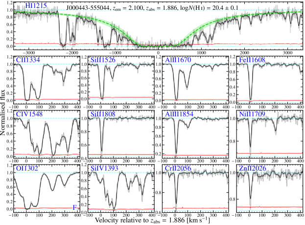
Figure 14: Example of a DLA in the DR1 spectrum of J000443$-$555044 that has not been previously reported (to our knowledge). Each panel shows the portion of spectrum (light grey histogram) covering the labelled transition in velocity space around a common redshift, $z_{\textrm{\scriptsize abs}}=1.886$. To aid visual inspection, the spectrum has been Gaussian-smoothed (shown in the black line). A single-component Voigt profile with an H i column density that best matches the $\textrm{Ly-}\alpha$ profile, $N_{\textsc{h\scriptsize{\,i}}}=10^{20.4\pm 0.1}$ $\textrm{cm}^{-2}$, is shown in the upper panel (green dashed line; shading indicates the $N_{\textsc{h\scriptsize{\,i}}}$ uncertainty). The “F” in the $\text{O\,{i}}\,\lambda\textrm{1302}$ panel indicates that is falls within the $\textrm{Ly-}\alpha$ forest.

The DR1 sample of 155 DLAs is the largest sample from a single high-resolution spectrograph to date. In this context it offers unprecedented opportunities for studying the range of chemical properties of DLAs, where the high resolution allows the detection and detailed modelling of the associated metal lines. However, it is important to note that a substantial proportion of UVES quasar observations specifically target quasars with known DLAs: Zafar et al. (2013b) searched the proposal titles and abstracts for references to DLAs for their sample of 250 UVES quasar spectra, finding that $\sim$45 were targeted due to specific, known DLAs. While this ensures a large DLA sample from the DR1 spectra, it also ensures the sample is biased: DLAs will be over-represented in the DR1 spectra and their column density, redshift and metallicity distributions should be interpreted cautiously as a result. Figure 15 illustrates the distribution of H i column densities and absorption redshifts in the DR1 DLA sample. The $z_{\textrm{\scriptsize abs}}$ distribution in the lower panel is clearly a strong function of the emission redshift distribution (Figure 1), but also the wavelength coverage and detectability of broad $\textrm{Ly-}\alpha$ lines; the following section (Section 6.2) details these aspects. The upper panel of Figure 15 compares the shape of the DR1 $\log(N_{\textsc{h\scriptsize{\,i}}}/\textrm{cm}^{-2})$ distribution with the Gamma function fit to that of the SDSS DLA survey by Noterdaeme et al. (2009). The fit has been scaled to yield a cumulative number of DLAs equal to the number in DR1. Overall, the relative representation of low and high $N_{\textsc{h\scriptsize{\,i}}}$ DLAs in DR1 approximately reflects the expectation from a blind survey. However, very high $N_{\textsc{h\scriptsize{\,i}}}$ DLAs are somewhat over-represented: there are 4 systems with $\log(N_{\textsc{h\scriptsize{\,i}}}/\textrm{cm}^{-2})\geq 21.7$ in DR1, while 0.8 are expected from the scaled fit from SDSS in Figure 15.

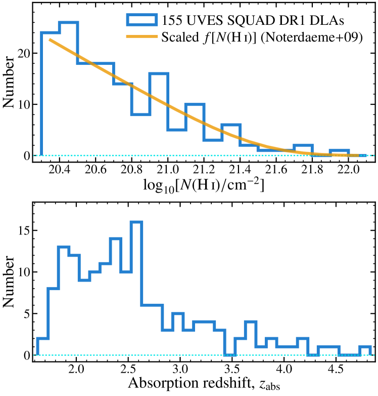
Figure 15: H i column density and absorption redshift distributions for the 155 DLAs identified in the final DR1 spectra. Because the original UVES observations often targeted known DLAs, they will be significantly over-represented in the DR1 spectra. The upper panel compares the $\log(N_{\textsc{h\scriptsize{\,i}}}/\textrm{cm}^{-2})$ distribution (histogram) shape with the Gamma function fit of the frequency distribution, $f(N_{\textsc{h\scriptsize{\,i}}})$, derived from the SDSS survey by Noterdaeme et al. (2009), scaled so that its integral for $\log(N_{\textsc{h\scriptsize{\,i}}}/\textrm{cm}^{-2})\geq 20.3$ is 155 (orange line). The absorption redshift ($z_{\textrm{\scriptsize abs}}$) distribution shown in the lower panel should be interpreted in conjunction with the emission redshift distribution in Figure 1 and the $\textrm{Ly-}\alpha$ detection sensitivity functions in Figs. 16 and 17.

6.2 Absorption line surveys

Figure 16 illustrates the total DR1 spectral coverage of strong absorption lines that are commonly surveyed in cosmological studies: H i $\textrm{Ly-}\alpha$, $\text{O\,{vi}}\,\lambda\textrm{1031}$, $\text{C\,{iv}}\,\lambda\textrm{1548}$, $\text{Mg\,{ii}}\,\lambda\textrm{2796}$, $\text{Si\,{iv}}\,\lambda\textrm{1393}$ and $\text{Ca\,{ii}}\,\lambda\textrm{3934}$. The metal lines occur in doublets and so are easily identified, especially in high-resolution spectra because their (identical) velocity structures are resolved. In Figure 16 only the strongest member of the doublets, as listed above, is considered. For H i $\textrm{Ly-}\alpha$, Figure 16 includes only the $\textrm{Ly-}\alpha$ forest, i.e. the redshift path between the $\textrm{Ly-}\alpha$ and $\textrm{Ly-}\beta$ quasar emission lines, and for O vi, which occurs only in the $\textrm{Ly-}\alpha$ forest, all redshifts up to the emission redshift are included. For C iv, Mg ii, Siiv and Ca ii, the redshift path extends down to the $\textrm{Ly-}\alpha$ emission line (or zero redshift, for Ca ii). Figure 16 also shows the total number of DR1 spectra that cover each transition at any redshift (in parentheses in the legends). For example, 68% of the spectra cover some part of the $\textrm{Ly-}\alpha$ forest, while almost all DR1 spectra cover Mg ii (457 of 467) and Ca ii (all but one of 467). Even with these simple considerations, it is clear from Figure 16 that the DR1 spectra provide an extensive dataset in which to survey absorption lines at high resolution.

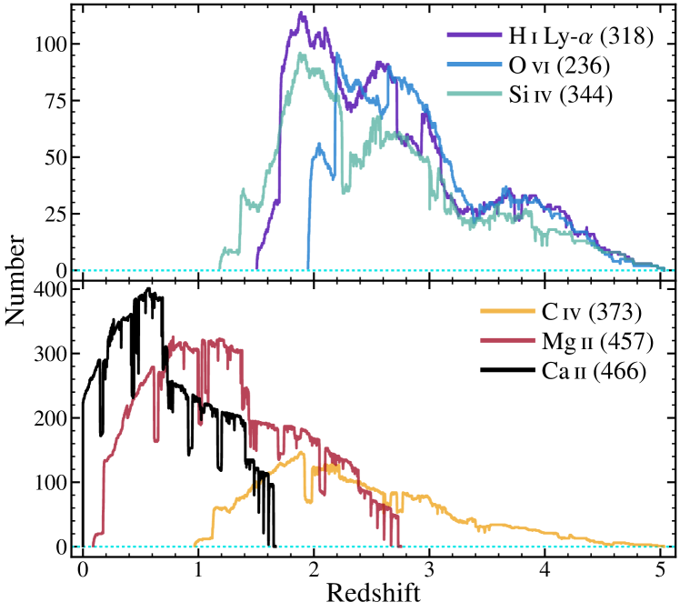
Figure 16: Number of DR1 quasar spectra covering the most commonly surveyed transitions as a function of redshift: H i $\textrm{Ly-}\alpha$, $\text{O\,{vi}}\,\lambda\textrm{1031}$, $\text{C\,{iv}}\,\lambda\textrm{1548}$, $\text{Mg\,{ii}}\,\lambda\textrm{2796}$, $\text{Si\,{iv}}\,\lambda\textrm{1393}$ and $\text{Ca\,{ii}}\,\lambda\textrm{3934}$. The total number of spectra covering each transition, integrated over all redshifts, is given in parentheses after the species label. Note the different vertical axis ranges for the top and bottom panels.

However, there are usually many other considerations required for statistical absorption line surveys in order to account for selection effects and biases. Typically, the redshift sensitivity function, $g(z)$, is a key metric: this is the total number of spectra in which the spectral feature being considered can, in principle, be detected once known selection effects are accounted for. That is, $g(z)$ is the spectral coverage of a given transition, or doublet, once additional detection effects are included, such as the S/N, proximity to quasar emission lines, telluric features and BALs that may preclude detection etc. Figure 17 presents $g(z)$ for the $\textrm{Ly-}\alpha$ forest region (regardless of the presence of DLAs and BALs), and the most commonly surveyed strong metal-line doublets outside the forest, i.e. C iv $\lambda\lambda$1548/1550, Mg ii $\lambda\lambda$2796/2803, Si iv $\lambda\lambda$1393/1402 and Ca ii $\lambda\lambda$3934/3969. Here, $g(z)$ masks out the strongest regions of telluric absorption (the O₂ and H₂O bands with $<$80% transmitted flux in Figure 8). For all species we excluded the region 3000 $\textrm{km\,s}^{-1}$ bluewards of the quasar emission redshift to avoid proximity effects from the quasar. For the metal doublets, $g(z)$ extends down to 3000 $\textrm{km\,s}^{-1}$ redwards of the $\textrm{Ly-}\alpha$ emission line, while for $\textrm{Ly-}\alpha$ it extends down to 3000 $\textrm{km\,s}^{-1}$ redwards of the $\textrm{Ly-}\beta$ emission line to avoid including $\textrm{Ly-}\beta$ absorption.

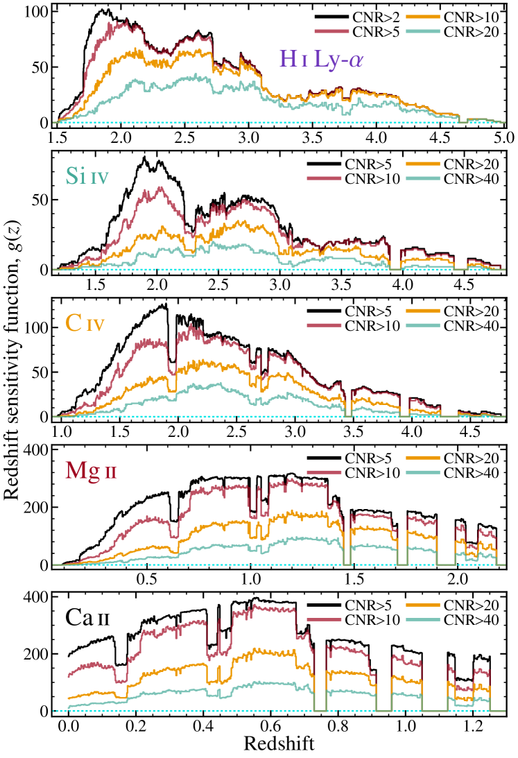
Figure 17: Total redshift sensitivity function, $g(z)$, of the DR1 spectra for H i $\textrm{Ly-}\alpha$ and the most commonly surveyed metal-line doublets outside the $\textrm{Ly-}\alpha$ forest: C iv $\lambda\lambda$1548/1550, Mg ii $\lambda\lambda$2796/2803, Si iv $\lambda\lambda$1393/1402 and Ca ii $\lambda\lambda$3934/3969. The strongest telluric absorption features (Figure 8) and the proximity zones near the relevant emission lines are excluded from $g(z)$, causing its shape to differ from the corresponding wavelength coverage function in Figure 16. $g(z)$ is calculated for four representative continuum-to-noise ratio (C/N) values for each species. This illustrates the large number of spectra in which relatively weak absorption lines can be detected.

The $g(z)$ functions in Figure 17 have broadly similar shapes and magnitudes to their raw wavelength coverage counterparts in Figure 16. However, avoiding the telluric and proximity regions reduces the number of sight-lines at all redshifts and reduces the sensitivity to zero for significant path lengths in the metal doublets, particularly Mg ii and Ca ii. To demonstrate how absorption line surveys will depend on the data quality, $g(z)$ is calculated for four representative C/N values for each species. This utilised the 1000-$\textrm{km\,s}^{-1}$-binned C/N maps of the quasar spectra described in Section 5.1.3. Note that the $g(z)$ functions in Figure 17 do not avoid other selection effects, such as broad absorption-line quasars, that some users should take into account for specific surveys. Finally, as is the case for DLAs (Section 6.1 above), many DR1 quasars were targeted for observations with UVES due to the presence of metal-line absorbers. We therefore urge caution in determining the incidence rates of such systems with the DR1 sample. However, the proposal names and abstracts for the original observations do not indicate targeting of specific, weak absorbers. That is, there is likely little or no such bias for absorbers with equivalent widths below the detection threshold for lower-resolution surveys (e.g. $\lesssim$0.2 Å for SDSS spectra). The $g(z)$ functions in Figure 17 indicate that very large redshift path lengths can be surveyed with the DR1 spectra, even for weak systems where higher C/N spectra are required (i.e. $\textrm{C/N}\geq 20$).

6.3 Time-variability studies using sub-spectra

The DR1 spectra were taken over a 16-year period, so they are potentially useful in constraining the time-variability of absorption systems. This is particularly relevant for both narrow and broad metal absorption lines associated with outflows from the quasar central engines and/or host galaxies, as these lines are often observed to vary on time-scales shorter than $\sim$10 years (e.g Hamann et al., 2011; Rodríguez Hidalgo et al., 2013). Amongst the 467 quasars with final DR1 spectra, 92 comprise exposures taken more than a year apart, and 11 were observed over more than a decade interval. Significantly time-variable absorption lines can be easily identified in the final spectra using the same methods used to identify artefacts in Section 4.2.1 (see Figure 3), particularly by using uves_popler to simultaneously view the flux and $\chi^{2}_{\nu}$ spectra.

Once time-variable absorption has been identified – or if it is suspected but higher S/N is required for detection – uves_popler includes a facility to create “sub-spectra” for comparative analyses: subsets of the original exposures can be selected for combination after the manual phase. This allows, for example, the best possible combination of exposures taken in one year to be compared with that from another year, and to identify or study time-variable absorption with the highest possible S/N in each case. The advantage of this approach is that sub-spectra are only split into separate spectra after being processed, cleaned, and continuum-fitted together; their treatment has been identical and observed differences between them are therefore more easily studied and interpreted. uves_popler sub-spectra have previously been employed in isolating instrumental systematic effects in UVES and HIRES spectra for studies of possible variations in the fine-structure constant and proton-to-electron mass ratio (e.g. Daprà et al., 2015; Murphy et al., 2016; Murphy & Cooksey, 2017). However, Figure 18 illustrates their utility in studying time-variability in a broad absorption-line system that is highly blueshifted with respect to the quasar, presumably due to a high-velocity outflow. A systematic search for, and study of, time-variable absorption lines in, e.g., BAL quasars could therefore be undertaken using the full DR1 data products in Murphy et al. (2018, i.e. both the final spectrum and the extracted, contributing exposures).

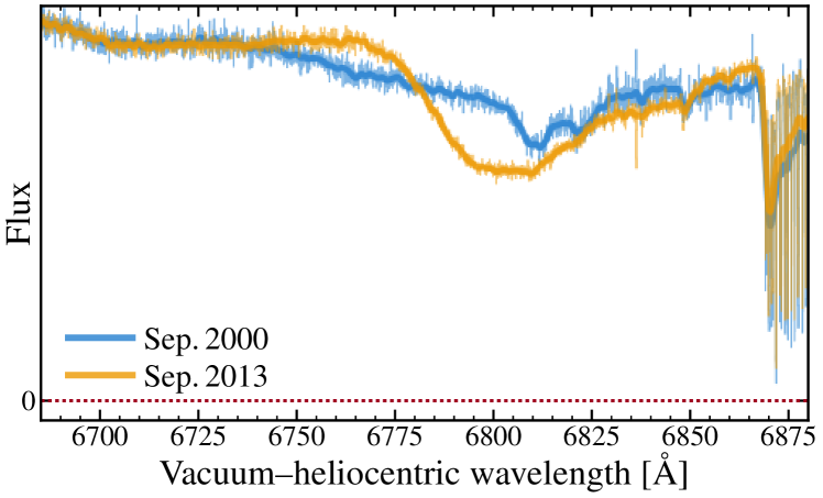
Figure 18: Example of a time-variable C iv broad absorption line feature $\sim$21000 $\textrm{km\,s}^{-1}$ bluewards of the emission redshift of J005758$-$264314. Two “sub-spectra” are shown (see text), comprising 11 and 13 exposures from Sep. 2000 and 2013, respectively. All exposures were combined to form the DR1 final spectrum of this quasar, but its $\chi^{2}_{\nu}$ spectrum (not shown) increases dramatically in the spectral region shown, sign-posting potential time-variable absorption. Each sub-spectrum (histograms) has been smoothed with a 10-pixel-wide Gaussian kernel for clarity (lines). Note that the absorption redwards of 6865 Å is the telluric O₂ B band.

7 Conclusions

We have presented the first data release of the UVES SQUAD: 475 quasars, 467 of which have final, combined spectra (see Table 1). This is the largest database of high-resolution quasar spectra. The DR1 spectra are fully reproducible – from the raw archival UVES exposures to final, combined and continuum-fitted spectra – with a few commands using open-source software. All reduced exposures and files required to produce the final spectra and figures in this paper are provided in Murphy et al. (2018). We also documented software tools for preparing and executing the UVES data reduction pipeline (uves_headsort; Murphy, 2016a), and for combining the extracted exposures of a quasar, and cleaning and continuum fitting the result (uves_popler; Murphy, 2016b). The latter tool enables users of the DR1 spectra to improve the spectra, or modify them for their particular projects; we encourage and welcome improvements in this way and can make them available in future data releases.

A primary motivation for constructing DR1 was to enable statistical analyses of large quasar and absorber samples, particularly those requiring high resolution spectra (e.g. weak metal lines). We highlighted three broad areas where the DR1 spectra may be especially useful: DLA studies, absorption-line surveys, and studies of variable absorption, particularly outflows from quasars. To assist DLA studies, we presented a catalogue of 155 DLAs whose $\textrm{Ly-}\alpha$ lines are recorded in the DR1 spectra, 18 of which have not been reported previously (see Table 3). The H i column densities from the literature are provided, plus values for the 18 new DLAs measured directly from the DR1 spectra. For absorption line surveys, the redshift sensitivity functions of the DR1 sample are presented in Figure 17 for the most commonly surveyed ionic species (H i, Si iv, C iv, Mg ii and Ca ii). Indeed, several absorption-line surveys have already been conducted using earlier, preliminary versions of the UVES SQUAD spectra (e.g. Richter et al., 2011; Ben Bekhti et al., 2012; Nielsen et al., 2013; Mas-Ribas et al., 2018; Mathes et al., 2018). To assist studies of variable absorption lines, the uves_popler software can be used to construct “sub-spectra”: sub-sets of exposures combined in the same way, with the same continuum, as the final spectrum. The highest S/N sub-spectra from different epochs can then be compared as accurately as possible. Finally, while we have invested considerable effort in cleaning all DR1 spectra to a minimum standard, many artefacts remain and are important to consider for such applications – see Section 5.2.

The second data release of UVES SQUAD is currently in preparation. It is anticipated to include spectra of another $\sim$180 quasars whose first exposure was taken between 30 June 2008 (the end date for first exposures in DR1) and early 2018. DR1 quasars with new exposures taken after 30 June 2008 will also be updated in DR2. While we have attempted to identify every quasar observed by UVES in the DR1 acquisition period (see Section 2), it remains possible that a small number may have escaped our selection criteria. We welcome knowledge of such quasars from the community and will include spectra of these in DR2 where possible.

Supporting Information

Additional Supporting Information may be found in the online version of this article and in Murphy et al. (2018):

DR1_quasars_master.csv. Complete version of Table 1, incorporating the DLA information from Table 3.
DR1_DLAs.pdf. Velocity plots of all 18 new DLAs reported in Table 3, similar to the example in Figure 14.

Please note: Oxford University Press are not responsible for the content or functionality of any supporting materials supplied by the authors. Any queries (other than missing material) should be directed to the corresponding author for the paper.

References

- Abolfathi et al. (2018) Abolfathi B. et al., 2018, ApJS, 235, 42
- Astropy Collaboration (2013) Astropy Collaboration, 2013, A&A, 558, A33
- Bagdonaite et al. (2014) Bagdonaite J., Ubachs W., Murphy M. T., Whitmore J. B., 2014, ApJ, 782, 10
- Becker et al. (2007) Becker G. D., Rauch M., Sargent W. L. W., 2007, ApJ, 662, 72
- Ben Bekhti et al. (2012) Ben Bekhti N., Winkel B., Richter P., Kerp J., Klein U., Murphy M. T., 2012, A&A, 542, A110
- Boera et al. (2014) Boera E., Murphy M. T., Becker G. D., Bolton J. S., 2014, MNRAS, 441, 1916
- Daprà et al. (2015) Daprà M., Bagdonaite J., Murphy M. T., Ubachs W., 2015, MNRAS, 454, 489
- Daprà et al. (2016) Daprà M., Niu M. L., Salumbides E. J., Murphy M. T., Ubachs W., 2016, ApJ, 826, 192
- Dekker et al. (2000) Dekker H., D’Odorico S., Kaufer A., Delabre B., Kotzlowski H., 2000, in Iye M., Moorwood A. F. M., eds, Proc. SPIE Vol. 4008. SPIE, pp 534–545, doi:10.1117/12.395512
- Dessauges-Zavadsky et al. (2001) Dessauges-Zavadsky M., D’Odorico S., McMahon R. G., Molaro P., Ledoux C., Péroux C., Storrie-Lombardi L. J., 2001, A&A, 370, 426
- Dessauges-Zavadsky et al. (2003) Dessauges-Zavadsky M., Péroux C., Kim T.-S., D’Odorico S., McMahon R. G., 2003, MNRAS, 345, 447
- Ellison et al. (2001) Ellison S. L., Yan L., Hook I. M., Pettini M., Wall J. V., Shaver P., 2001, A&A, 379, 393
- Ellison et al. (2010) Ellison S. L., Prochaska J. X., Hennawi J., Lopez S., Usher C., Wolfe A. M., Russell D. M., Benn C. R., 2010, MNRAS, 406, 1435
- Evans et al. (2014) Evans T. M. et al., 2014, MNRAS, 445, 128
- Flesch (2015) Flesch E. W., 2015, PASA, 32, e010
- Guimarães et al. (2012) Guimarães R., Noterdaeme P., Petitjean P., Ledoux C., Srianand R., Lopez S., Rahmani H., 2012, AJ, 143, 147
- Hamann et al. (2011) Hamann F., Kanekar N., Prochaska J. X., Murphy M. T., Ellison S., Malec A. L., Milutinovic N., Ubachs W., 2011, MNRAS, 410, 1957
- Hambly et al. (2001) Hambly N. C. et al., 2001, MNRAS, 326, 1279
- Hunter (2007) Hunter J. D., 2007, Computing in Science and Engineering, 9, 90
- Kim et al. (2004) Kim T.-S., Viel M., Haehnelt M. G., Carswell R. F., Cristiani S., 2004, MNRAS, 347, 355
- King et al. (2008) King J. A., Webb J. K., Murphy M. T., Carswell R. F., 2008, Phys. Rev. Lett., 101, 251304
- King et al. (2012) King J. A., Webb J. K., Murphy M. T., Flambaum V. V., Carswell R. F., Bainbridge M. B., Wilczynska M. R., Koch F. E., 2012, MNRAS, 422, 3370
- Kotuš et al. (2017) Kotuš S. M., Murphy M. T., Carswell R. F., 2017, MNRAS, 464, 3679
- Ledoux et al. (2003) Ledoux C., Petitjean P., Srianand R., 2003, MNRAS, 346, 209
- Ledoux et al. (2006) Ledoux C., Petitjean P., Fynbo J. P. U., Møller P., Srianand R., 2006, A&A, 457, 71
- Ledoux et al. (2015) Ledoux C., Noterdaeme P., Petitjean P., Srianand R., 2015, A&A, 580, A8
- Liske (2014) Liske J., 2014, vpguess: Fitting multiple Voigt profiles to spectroscopic data, Astrophysics Source Code Library (ascl:1408.016)
- Mas-Ribas et al. (2018) Mas-Ribas L., Riemer-Sørensen S., Hennawi J. F., Miralda-Escudé J., O’Meara J. M., Pérez-Ràfols I., Murphy M. T., Webb J. K., 2018, ApJ, 862, 50
- Mathes et al. (2018) Mathes N. L., Churchill C. W., Murphy M. T., 2018, ApJ, submitted, arXiv:1701.05624,
- Molaro et al. (2000) Molaro P., Bonifacio P., Centurión M., D’Odorico S., Vladilo G., Santin P., Di Marcantonio P., 2000, ApJ, 541, 54
- Molaro et al. (2013) Molaro P. et al., 2013, A&A, 555, A68
- Murphy (2016a) Murphy M. T., 2016a, UVES_headsort: VLT/UVES pipeline preparation, doi:10.5281/zenodo.44766
- Murphy (2016b) Murphy M. T., 2016b, UVES_popler: POst PipeLine Echelle Reduction software, doi:10.5281/zenodo.44765
- Murphy & Bernet (2016) Murphy M. T., Bernet M. L., 2016, MNRAS, 455, 1043
- Murphy & Cooksey (2017) Murphy M. T., Cooksey K. L., 2017, MNRAS, 471, 4930
- Murphy et al. (2007) Murphy M. T., Tzanavaris P., Webb J. K., Lovis C., 2007, MNRAS, 378, 221
- Murphy et al. (2016) Murphy M. T., Malec A. L., Prochaska J. X., 2016, MNRAS, 461, 2461
- Murphy et al. (2018) Murphy M. T., Kacprzak G. G., Savorgnan G. A. D., Carswell R. F., 2018, UVES SQUAD Data Release 1, doi:10.5281/zenodo.1345974 https://github.com/MTMurphy77/UVES_SQUAD_DR1
- Nielsen et al. (2013) Nielsen N. M., Churchill C. W., Kacprzak G. G., Murphy M. T., 2013, ApJ, 776, 114
- Noterdaeme et al. (2008) Noterdaeme P., Ledoux C., Petitjean P., Srianand R., 2008, A&A, 481, 327
- Noterdaeme et al. (2009) Noterdaeme P., Petitjean P., Ledoux C., Srianand R., 2009, A&A, 505, 1087
- Noterdaeme et al. (2011) Noterdaeme P., Petitjean P., Srianand R., Ledoux C., López S., 2011, A&A, 526, L7
- Noterdaeme et al. (2015) Noterdaeme P., Srianand R., Rahmani H., Petitjean P., Pâris I., Ledoux C., Gupta N., López S., 2015, A&A, 577, A24
- Noterdaeme et al. (2017) Noterdaeme P. et al., 2017, A&A, 597, A82
- O’Meara et al. (2015) O’Meara J. M. et al., 2015, AJ, 150, 111
- O’Meara et al. (2017) O’Meara J. M., Lehner N., Howk J. C., Prochaska J. X., Fox A. J., Peeples M. S., Tumlinson J., O’Shea B. W., 2017, AJ, 154, 114
- Pâris et al. (2018) Pâris I. et al., 2018, A&A, 613, A51
- Parks et al. (2018) Parks D., Prochaska J. X., Dong S., Cai Z., 2018, MNRAS, 476, 1151
- Penprase et al. (2010) Penprase B. E., Prochaska J. X., Sargent W. L. W., Toro-Martinez I., Beeler D. J., 2010, ApJ, 721, 1
- Péroux et al. (2001) Péroux C., Storrie-Lombardi L. J., McMahon R. G., Irwin M., Hook I. M., 2001, AJ, 121, 1799
- Péroux et al. (2005) Péroux C., Dessauges-Zavadsky M., D’Odorico S., Sun Kim T., McMahon R. G., 2005, MNRAS, 363, 479
- Petitjean et al. (2000) Petitjean P., Srianand R., Ledoux C., 2000, A&A, 364, L26
- Pettini & Cooke (2012) Pettini M., Cooke R., 2012, MNRAS, 425, 2477
- Pettini et al. (2002) Pettini M., Ellison S. L., Bergeron J., Petitjean P., 2002, A&A, 391, 21
- Pettini et al. (2008a) Pettini M., Zych B. J., Steidel C. C., Chaffee F. H., 2008a, MNRAS, 385, 2011
- Pettini et al. (2008b) Pettini M., Zych B. J., Murphy M. T., Lewis A., Steidel C. C., 2008b, MNRAS, 391, 1499
- Prochaska & Wolfe (1999) Prochaska J. X., Wolfe A. M., 1999, ApJS, 121, 369
- Prochaska & Wolfe (2009) Prochaska J. X., Wolfe A. M., 2009, ApJ, 696, 1543
- Prochaska et al. (2001) Prochaska J. X. et al., 2001, ApJS, 137, 21
- Prochaska et al. (2003a) Prochaska J. X., Gawiser E., Wolfe A. M., Cooke J., Gelino D., 2003a, ApJS, 147, 227
- Prochaska et al. (2003b) Prochaska J. X., Gawiser E., Wolfe A. M., Castro S., Djorgovski S. G., 2003b, ApJ, 595, L9
- Prochaska et al. (2005) Prochaska J. X., Herbert-Fort S., Wolfe A. M., 2005, ApJ, 635, 123
- Prochaska et al. (2007) Prochaska J. X., Wolfe A. M., Howk J. C., Gawiser E., Burles S. M., Cooke J., 2007, ApJS, 171, 29
- Prochaska et al. (2008) Prochaska J. X., Hennawi J. F., Herbert-Fort S., 2008, ApJ, 675, 1002
- Quast et al. (2004) Quast R., Reimers D., Levshakov S. A., 2004, A&A, 415, L7
- Rahmani et al. (2013) Rahmani H. et al., 2013, MNRAS, 435, 861
- Richter et al. (2011) Richter P., Krause F., Fechner C., Charlton J. C., Murphy M. T., 2011, A&A, 528, A12
- Riemer-Sørensen et al. (2017) Riemer-Sørensen S., Kotuš S., Webb J. K., Ali K., Dumont V., Murphy M. T., Carswell R. F., 2017, MNRAS, 468, 3239
- Rodríguez Hidalgo et al. (2013) Rodríguez Hidalgo P., Eracleous M., Charlton J., Hamann F., Murphy M. T., Nestor D., 2013, ApJ, 775, 14
- Schaye et al. (2003) Schaye J., Aguirre A., Kim T.-S., Theuns T., Rauch M., Sargent W. L. W., 2003, ApJ, 596, 768
- Srianand et al. (2008) Srianand R., Noterdaeme P., Ledoux C., Petitjean P., 2008, A&A, 482, L39
- Vanden Berk et al. (2001) Vanden Berk D. E. et al., 2001, AJ, 122, 549
- Vogt et al. (1994) Vogt S. S. et al., 1994, Proc. SPIE Instrumentation in Astronomy VIII, 2198, 362
- Wells et al. (1981) Wells D. C., Greisen E. W., Harten R. H., 1981, Astronomy and Astrophysics Supplement, 44, 363
- Whitmore & Murphy (2015) Whitmore J. B., Murphy M. T., 2015, MNRAS, 447, 446
- Whitmore et al. (2010) Whitmore J. B., Murphy M. T., Griest K., 2010, ApJ, 723, 89
- Wolfe et al. (1981) Wolfe A. M., Briggs F. H., Jauncey D. L., 1981, ApJ, 248, 460
- Wolfe et al. (2005) Wolfe A. M., Gawiser E., Prochaska J. X., 2005, Annual Review of Astronomy and Astrophysics, 43, 861
- Wolfe et al. (2008) Wolfe A. M., Prochaska J. X., Jorgenson R. A., Rafelski M., 2008, ApJ, 681, 881
- Zafar et al. (2013a) Zafar T., Popping A., Péroux C., 2013a, A&A, 556, A140
- Zafar et al. (2013b) Zafar T., Péroux C., Popping A., Milliard B., Deharveng J.-M., Frank S., 2013b, A&A, 556, A141