Distribution of a tagged particle position in the one-dimensional symmetric simple exclusion process with two-sided Bernoulli initial condition

Abstract

For the two-sided Bernoulli initial condition with density $\rho_{-}$ (resp. $\rho_{+}$) to the left (resp. to the right), we study the distribution of a tagged particle in the one dimensional symmetric simple exclusion process. We obtain a formula for the moment generating function of the associated current in terms of a Fredholm determinant. Our arguments are based on a combination of techniques from integrable probability which have been developed recently for studying the asymmetric exclusion process and a subsequent intricate symmetric limit. An expression for the large deviation function of the tagged particle position is obtained, including the case of the stationary measure with uniform density $\rho$.

1 Introduction and results

1.1 The exclusion process and a tagged particle

The asymmetric simple exclusion process (ASEP) is a continuous time interacting particles Markov process $\eta(t)=\{\eta_{x}(t),x\in\mathbb{Z}\}$, in which each particle is located on a discrete site labeled by an integer $x\in{\mathbb{Z}}$ and can hop to its right or left nearest neighboring site with rate $p$ or $q$ respectively, where $0\leq p,q\leq 1,p+q>0$. Due to the volume exclusion, jumps to an occupied site are forbidden. The state of the ASEP, $\eta=\{\eta_{x}\}_{x\in\mathbb{Z}}$, is a collection of $\eta_{x}$ which is the occupation at $x$, i.e., $\eta_{x}=1$(resp. 0) when the site $x$ is occupied (resp. empty). Formally the ASEP is defined through the generator,

$$Lf=\sum_{x\in\mathbb{Z}}(p\eta_{x}(1-\eta_{x+1})+q(1-\eta_{x})\eta_{x+1})[f(\eta^{x,x+1})-f(\eta)],$$ (1.1)

where $\eta^{x,x+1}$ denotes the state with $\eta_{x},\eta_{x+1}$ swapped in $\eta$, and $f$ is a cylinder function. For the precise construction of the process, see [33, 34]. The asymmetry parameter is defined as $\tau=p/q$ and in this paper we follow the convention of [44, 7] in which particles hop preferably towards the left, i.e., $0\leq\tau\leq 1$. Accordingly, a current flowing from right to left will be counted positively.

The symmetric simple exclusion process (SEP) corresponds to the case where the jumps are isotropic; the hopping rates are equal and set to $p=q=1$. In this work, we shall focus on the motion of a tagged particle (or tracer) in the SEP. Because of the exclusion condition, particles move and conserve their ordering. The SEP is therefore a pristine model of single file diffusion [36, 2, 49] and has a lot of applications in physics, see for instance [29, 38] for recent references.

The long time behavior of the tracer $X_{t}$ has been the subject of many studies since Spitzer’s original paper [42]. In particular, for a system initially at equilibrium with uniform density $\rho$, Arratia [3], Rost and Vares [37] and De Masi and Ferrari [11] proved that the variance of the position $X_{t}$ at time $t$ of the tracer grows subdiffusively with time as $t^{1/2}$ and further that the rescaled variable $t^{-1/4}X_{t}$ converges to a Gaussian with variance $\sigma_{X}^{2}=\frac{2(1-\rho)}{\rho\sqrt{\pi}}$. Moreover, Peligrad and Sethuraman [35] have established the generalization (see for instance [43], Chapter 6, Conjecture 6.5 page 294) that the rescaled process weakly converges to a fractional Brownian motion ${\mathbb{B}}_{1/4}(t)$ with Hurst parameter 1/4,

$$\sigma_{X}^{-1}\lambda^{-1/4}X_{\lambda t}\Rightarrow{\mathbb{B}}_{1/4}(t).$$

For an initial setting out of equilibrium, that corresponds to a non-uniform initial distribution of the particles, Jara and Landim [24] have obtained laws of large numbers and central limit theorems for local equilibrium initial settings. The former reads

$$\frac{X_{t}}{\sqrt{4t}}\to-\xi_{0}$$ (1.2)

as $t\to\infty$ in probability with the value of $\xi_{0}$ being given by

$$\int_{0}^{\infty}(\rho(x,t)-\rho(x,0))dx=\int_{0}^{-\xi_{0}}\rho(x,t)dx.$$ (1.3)

Here $\rho(x,t)$ is the solution to the hydrodynamic equation, which for the case of SEP is simply given by the diffusion equation (see for instance [26]).

1.2 Large deviation for a tagged particle

More recently, Sethuraman and Varadhan [41] have established the large deviation principle for a tagged particle in SEP. (For general information about large deviation theory, see for instance [12, 13, 48].) They considered two classes of initial conditions – either deterministic configurations or local equilibrium measures that interpolate between a density $\rho_{-}$ when $x\to-\infty$ and $\rho_{+}$ when $x\to+\infty$ – and proved that there exists a large deviation (or good rate) function $\phi(\xi)$, i.e., a function on $\mathbb{R}$ such that for each $a\in[0,\infty)$, the set $\{\xi:\phi(\xi)\leq a\}$ is closed and compact, and the following property holds

$$\quad-\inf_{\xi\in\bar{U}}\phi(\xi)\geq\limsup_{t\to\infty}t^{-1/2}\text{Prob}\left(-\frac{X_{t}}{\sqrt{4t}}\in U\right)$$

$$\geq\liminf_{t\to\infty}t^{-1/2}\text{Prob}\left(-\frac{X_{t}}{\sqrt{4t}}\in U\right)\geq-\inf_{\xi\in U^{\circ}}\phi(\xi),$$ (1.4)

where $U$ is a Borel set of $\mathbb{R}$, $U^{\circ}$ denotes its interior, $\bar{U}$ its closure. Since our main interest in the paper is the explicit calculation of the rate function, we will write this statement more heuristically as

$$\text{Prob}\left(\frac{X_{t}}{\sqrt{4t}}=-\xi\right)\simeq\exp[-\sqrt{t}\phi(\xi)].$$ (1.5)

Here the left hand side is an abuse of notation for the probability $\text{Prob}\left(-\frac{X_{t}}{\sqrt{4t}}\in(\xi,\xi+d\xi]\right)$ and equalities with the symbol $\simeq$ have to be understood at the level of dominant exponential terms, e.g., (1.5) means $\lim_{t\to\infty}\frac{-1}{\sqrt{t}}\log\Big{[}\text{Prob}\left(-\frac{X_{t}}{\sqrt{4t}}\in(\xi,\xi+d\xi]\right)/d\xi\Big{]}=\phi(\xi)$, provided that the probability density exists for the probability on left hand side. For use of this kind of notation, see for instance remarks in Appendix B of [47].

The authors in [41] found an expression of the rate function $\phi(\xi)$ in terms of that for the process empirical density, which we recall here. Let $M_{1}=M_{1}(\rho_{-},\rho_{+})$ denote the space of functions which equals $\rho_{-}$ (resp. $\rho_{+}$) for all $x\leq x_{*}$ (resp. $x\geq x^{*}$) for some $x_{*}\leq x^{*}$, $D(M_{1};[0,T])$ the set of right continuous trajectories on $M_{1}$ with left limits, and $C_{K}^{2,1}(\mathbb{R}\times[0,T])$ the space of compactly supported functions twice and once continuously differentiable in $x$ and $t$. For $\mu\in D(M_{1},[0,T])$, let us define the linear functional on $C_{K}^{2,1}(\mathbb{R}\times[0,T])$,

$$l(\mu;G)=\int G(x,T)\mu_{T}(x)dx-\int G(x,0)\mu_{0}(x)dx-\int_{0}^{T}\int\mu_{t}(x)\left(\frac{\partial}{\partial t}+\frac{1}{2}\frac{\partial^{2}}{\partial x^{2}}\right)G(x,t)dxdt,$$ (1.6)

where $\mu_{t}(x)=\mu(x,t)$ and $G\in C_{K}^{2,1}(\mathbb{R}\times[0,T])$. Besides, the process empirical density is defined by

$$\mu^{N}(s,x,\eta)=\sum_{k\in\mathbb{Z}}\eta_{k}(N^{2}s)1_{[k/N,(k+1)/N)}(x)$$ (1.7)

where $x\in\mathbb{R},s\in[0,T),0<T<\infty$ and $N$ is a large integer tending to infinity. The results of [27, 41] (Corollary 1.4 in [41]) say that for the process starting from a local equilibrium measure, corresponding to a density profile $\gamma\in M_{1}$, the large deviation principle holds and that the rate function $I(\mu)$ for the process empirical density is given by

$$I(\mu)=I_{0}(\mu)+h(\mu_{0};\gamma)$$ (1.8)

where

$$I_{0}(\mu) =\sup_{G\in C_{K}^{2,1}(\mathbb{R}\times[0,T])}\left\{l(\mu;G)-\frac{1}{2}\int_{0}^{T}\int\mu_{t}(1-\mu_{t})G_{x}^{2}(x,t)dxdt\right\},$$ (1.9)

$$h(\mu_{0};\gamma) =\sup_{\phi_{0},\phi_{1}\in C_{K}(\mathbb{R})}\left\{\int\mu_{0}(x)\phi_{0}(x)dx+\int(1-\mu_{0}(x))\phi_{1}(x)dx\right.$$ (1.10)

$$\quad\left.-\int\log[\gamma(x)e^{\phi_{0}(x)}+(1-\gamma(x))e^{\phi_{1}(x)}]\right\}.$$ (1.11)

Here $C_{K}(\mathbb{R})$ is the space of compactly supported continuous functions. Then it was shown in [41] (Theorem 1.5) that the rate function $\phi(\xi)$ for the tagged particle is given in terms of $I(\mu)$ by

$$\phi(\xi)=\inf_{\mu\in D(M_{1},[0,T])}\left\{I(\mu):\int_{0}^{\infty}(\mu_{T}(x)-\mu_{0}(x))dx=\int_{0}^{-\xi}\mu_{T}(x)dx\right\}.$$ (1.12)

By using the representation above, the authors of [41] have given some bounds on the rate function, studied its asymptotic growth and its behavior near its vanishing minimum $\phi(\xi_{0})=0$, which is attained when $\mu_{t}(x)$ becomes $\rho(x,t)$ in (1.3), i.e., at $\xi_{0}$ given by (1.2).

In this article we shall calculate explicitly the rate function $\phi(\xi)$ when the system is prepared in a step initial profile with densities $\rho_{-}$ and $\rho_{+}$ on the left and on the right of the origin where the tracer is initially located. In fact we will find a formula for the distribution of the tagged particle for finite $t$ and $x$. Then, the rate function $\phi(\xi)$ will be extracted rather straightforwardly from it.

Knowing the large deviation function $\phi$ will allow us to compute the cumulants of the tracer’s position $X_{t}$ in the limit $t\to\infty$. These results have been announced in the letter [20] and the purpose of the present work is to provide the reader with proofs of our claims and some generalizations of our results. Besides the derivations of our results have been simplified considerably and we present here these improved arguments.

1.3 Current and height variables

1.3.1 Definition

To study properties of the tagged particle position $X_{t}$, it is useful to consider a related quantity, $Q(x,t)$, which is the time-integrated current that has flown through the bond $(x,x+1)$ between time 0 and $t$, i.e. $Q(x,t)$ is equal to the total number of particles that have jumped from $x+1$ to $x$ minus the total number of particles that have jumped from $x$ to $x+1$ during the time interval $(0,t)$.

Let us define also the local height function $N(x,t)$ over the site $x$ at time $t$ by

$$N(x,t)=N_{t}+\begin{cases}+\sum_{y=1}^{x}\eta_{y}(t)\,,&x>0,\\ 0,&x=0,\\ -\sum_{y=x+1}^{0}\eta_{y}(t)\,,&x<0,\end{cases}$$ (1.13)

where $N_{t}=Q(0,t)$ is another notation for the time-integrated current through the bond $(0,1)$ during the time interval $[0,t]$.

Remark. In the usual mapping between the exclusion process in one-dimension and a fluctuating interface in a solid-on-solid model, it is the function $h(x,t)=N(x,t)-x/2$ that is defined as the local height of the interface. For the case of asymmetric hoppings, in a scaling limit, the interface $h(x,t)$ satisfies the Kardar-Parisi-Zhang equation [5].

By particle conservation, $Q(x,t)$ and $N(x,t)$ are related as follows: At $x=0$, $Q(0,t)=N(0,t)=N_{t}$. For $x>0$, $Q(x,t)=Q(0,t)+\sum_{y=1}^{x}\big{(}\eta_{y}(t)-\eta_{y}(0)\big{)}$ or equivalently

$$N(x,t)=Q(x,t)+\sum_{y=1}^{x}\eta_{y}(0)\,.$$ (1.14)

And for $x<0$,

$$N(x,t)=Q(x,t)-\sum_{y=x+1}^{0}\eta_{y}(0)\,.$$ (1.15)

In this article we focus on the two-sided Bernoulli initial condition: initially all sites are independent, a site with $x<0$ is occupied with probability $\rho_{-}$ and a site $x\geq 0$ is occupied with probability $\rho_{+}$.

For this initial condition, the current $Q(x,t)$ and the local height $N(x,t)$ satisfy some simple properties under symmetries that leave the SEP dynamics invariant [15]. In particular, spatial parity (i.e. left-right symmetry) implies

$$N(-x,t,\rho_{+},\rho_{-})\overset{d}{=}-N(x,t,\rho_{-},\rho_{+})$$ (1.16)

where $\overset{d}{=}$ means the equality in distribution and, for clarity sake, we have written explicitly the dependence on boundary densities. Similarly, from particle-hole conjugation, we have $Q(x,t,\rho_{+},\rho_{-})\overset{d}{=}-Q(x,t,1-\rho_{+},1-\rho_{-})$, and therefore

$$N(x,t,\rho_{+},\rho_{-})\overset{d}{=}x-N(x,t,1-\rho_{+},1-\rho_{-}).$$ (1.17)

1.3.2 Relation between the local height and the tracer’s position

At time $t=0$, we tag the particle which is closest to the origin from the right and call it the ’tracer’. Its initial position is $X_{0}\geq 0$ and its position at time $t$ is denoted by $X_{t}$. Using particle number conservation, the probability distribution of the position $X_{t}$ of a tagged particle is related to the distribution of the local height function $N(x,t)$ by the following identity

$${\quad\mathbb{P}[X_{t}\leq x]=\mathbb{P}[N(x,t)>0]}\,.$$ (1.18)

This formula will allow us to derive the statistical properties of $X_{t}$ from those of $N(x,t)$, which are more tractable because the height functions are local observables contrarily to $X_{t}$, which is drifting away with time. We recall how one finds Eq. (1.18) for completeness sake [20]. Consider a site $x>X_{0}$, located to the right of the initial position of the tracer. For the tracer $X_{t}$ to be strictly to the right of $x$ at time $t$, it is necessary that all the particles that were initially between $X_{0}$ and $x$ have crossed the bond $(x,x+1)$ from left to right. This means that the total current $Q(x,t)$ at $x$ has to be less than $-\sum_{i=X_{0}}^{x}\eta_{i}(0)=-\sum_{i=1}^{x}\eta_{i}(0)$ (using the fact that all sites between 1 and $X_{0}-1$ are empty at $t=0$). Hence, for $x\geq X_{0}$, we have

$$\hbox{Prob}\left(X_{t}>x\right) = \hbox{Prob}\left(Q(x,t)\leq-\sum_{i=1}^{x}\eta_{i}(0)\right)$$ (1.19)

$$= \hbox{Prob}\left(N(x,t)\leq 0\right)\,.$$

This equation is equivalent to (1.18).

More generally, at $t=0$, once the particle closest to the origin in the region $x\geq 0$ is selected as the tracer, all the particles in the system can be labeled as :

$$\ldots<X_{2}<X_{1}<X_{0}<X_{-1}<X_{-2}<\ldots$$

Then, the position $X_{m}(t)$ of the $m$-th tagged particle at time $t$ is related to the local height variables as follows :

$$\mathbb{P}[X_{m}(t)\leq x] =\mathbb{P}[N(x,t)\geq m]\,.$$

1.3.3 Large deviation for the current and the height

In [41], the authors have shown that in the long-time limit, the current $Q(x,t)$ satisfies the large deviation principle

$$\mathbb{P}\left(\frac{Q(x,t)}{\sqrt{t}}=q\right)\simeq\exp[-\sqrt{t}\Psi(\xi,q)]\,\,\,\,\hbox{ with }\,\,\,\,\xi=-\frac{x}{\sqrt{4t}},$$ (1.21)

where $\Psi(\xi,q)$ is the rate function of $Q(x,t)$. They also gave a formula for the large deviation function for the current in terms of the rate function for the process empirical measure $I(\mu)$ in (1.8) to be

$$\Psi(\xi,q)=\inf\left\{I(\mu):\int_{-\xi}^{\infty}(\mu_{T}(x)-\mu_{0}(x))dx=q\right\}.$$ (1.22)

The above statement was made only for $x=0$ case in [41]. It also holds for general $x$ by translational invariance.

By applying the same arguments, one can show that the height $N(x,t)$ also satisfies the large deviation principle

$$\mathbb{P}\left(\frac{N(x,t)}{\sqrt{t}}=q\right)\simeq\exp[-\sqrt{t}\Phi(\xi,q)]\,\,\,\,\hbox{ with }\,\,\,\,\xi=-\frac{x}{\sqrt{4t}}$$ (1.23)

where $\Phi(\xi,q)$ is the rate function of the local height variable $N(x,t)$. In addition, in terms of $I(\mu)$ this can be written as

$$\Phi(\xi,q)=\inf\left\{I(\mu):\int_{-\xi}^{\infty}(\mu_{T}(x)-\mu_{0}(x))dx+\int_{0}^{-\xi}\mu_{0}(x)dx=q\right\}.$$ (1.24)

Let us denote the expectation value by the bracket $\langle\cdots\rangle$. The characteristic function of $N(x,t)$ is defined as $\langle e^{\lambda N(x,t)}\rangle$ for all $\lambda\in\mathbb{R}$, – indeed, by using (LABEL:Mth-Tracer) and ignoring the exclusion condition, we note that the tails of the distribution of $N(x,t)$ are bounded above by a Gaussian. (Moreover we will find an explicit expression for this function which admits an analytic continuation to $\lambda\in\mathbb{C}$.) By taking derivatives with respect to $\lambda$ (assuming smoothness), the characteristic function generates all the moments of the random variable $N(x,t)$. By Varadhan’s lemma, see for instance Section 4.3 in [12], the large deviation principle (1.23) implies that the characteristic function behaves as

$$\langle e^{\lambda N(x,t)}\rangle\simeq e^{-\sqrt{t}\mu(\xi,\lambda)}\quad\hbox{ for}~{}\lambda\in\mathbb{R}~{}{\rm and}~{}t\to\infty\,.$$ (1.25)

The asymptotic cumulant generating function $\mu(\xi,\lambda)$ and the rate function $\Phi(\xi,q)$ are related by a Fenchel-Legendre transform :

$$\Phi(\xi,q)=\max_{\lambda}\left(\mu(\xi,\lambda)+\lambda q\right).$$ (1.26)

1.4 Exact expressions of the generating function and cumulants

1.4.1 Finite time formula

The central result of this work is an exact expression for the characteristic function of $N(x,t)$ valid for any finite values of $x$ and $t$, that can be expressed in terms of a Fredholm determinant.

Theorem 1.1.

For the two-sided Bernoulli initial condition with density $\rho_{-}$ (resp. $\rho_{+}$) to the left (resp. right), the characteristic function of $N(x,t),x\in\mathbb{Z},t\geq 0$, defined in (1.13) can be written as

$$\langle e^{\lambda N(x,t)}\rangle=\det(1+\omega K_{x,t})_{L^{2}(C_{0})}\cdot M_{0}(\lambda),$$ (1.27)

where the determinant on the right hand side is a Fredholm determinant with the kernel,

$$K_{x,t}(\xi_{1},\xi_{2})=\frac{\xi_{1}^{|x|}e^{\varepsilon(\xi_{1})t}}{\xi_{1}\xi_{2}+1-2\xi_{2}},$$ (1.28)

$$\omega=\rho_{+}(e^{\lambda}-1)+\rho_{-}(e^{-\lambda}-1)+\rho_{+}\rho_{-}(e^{\lambda}-1)(e^{-\lambda}-1),$$ (1.29)

and

$$M_{0}(\lambda) = \begin{cases}\left(1+\rho_{+}(e^{\lambda}-1)\right)^{x}\quad\quad{\rm for}\quad&x\geq 0,\\ \left(1+\rho_{-}(e^{-\lambda}-1)\right)^{-x}\quad\rm{for}\quad&x<0.\end{cases}$$ (1.30)

Here $\varepsilon(\xi)=\xi+1/\xi-2$ and $C_{0}$ is a contour around the origin with the radius small enough so that it does not include the poles from the denominator of the kernel (1.28).

Remark. The characteristic function $\langle e^{\lambda N(x,t)}\rangle$ on the left hand side is originally defined for $\lambda\in\mathbb{R}$. But the kernel $K_{x,t}$ being smooth in the vicinity of the small contour $C_{0}$, the corresponding operator is trace-class ([31], page 345) and therefore the Fredholm determinant (1.27) on the right hand side is well defined for all values of $\omega$ [4, 45], or equivalently for all values of $0\leq\rho_{\pm}\leq 1,\lambda\in\mathbb{C}$.

The key for the proof of the above theorem is the following formula for the moments of $N(x,t)$.

Proposition 1.2.

For $x\geq 0,t\geq 0$, the $n$-th moment of $N(x,t)$ is given by

$$\langle N(x,t)^{n}\rangle=\sum_{k=0}^{n}m_{n,k}J_{k}(x,t),$$ (1.31)

where $m_{n,k}$ is defined through

$$\sum_{n=0}^{\infty}\frac{\lambda^{n}}{n!}m_{n,k}=\frac{\omega^{k}}{k!}(1+\rho_{+}(e^{\lambda}-1))^{x}$$ (1.32)

and $J_{k}(x,t)$ is given by

$$J_{k}=J_{k}(x,t)=\int_{C_{0}}\cdots\int_{C_{0}}\prod_{i<j}\frac{\xi_{i}-\xi_{j}}{1+\xi_{i}\xi_{j}-2\xi_{j}}\prod_{i=1}^{k}\frac{\xi_{i}^{x}e^{\varepsilon(\xi_{i})t}}{(1-\xi_{i})^{2}}d\xi_{i}.$$ (1.33)

Here $\varepsilon(\xi)$ and $C_{0}$ are the same as in Theorem 1.1. The expression for $x<0$ case is found by applying the symmetry (1.16).

We will prove this proposition by first considering a $\tau$-deformed moment for the ASEP in Section 2 and then taking the symmetric limit in Section 3. To prove Theorem 1.1 we also need

Proposition 1.3.

The generating function of the integrals $\{J_{n}\}_{n\in\mathbb{N}}$ can be expressed as a Fredholm determinant

$$\sum_{n=0}^{\infty}\frac{\zeta^{n}}{n!}J_{n}=\det(1+\zeta K_{x,t})_{L^{2}(C_{0})},$$ (1.34)

where $\zeta\in\mathbb{C}$ and $K_{x,t}$ and $C_{0}$ are as explained in Theorem 1.1.

The proof of this proposition will be given in Section 4. Using Propositions 1.2 and 1.3, Theorem 1.1 is readily proved.

Proof of Theorem 1.1. For $x\geq 0$ we have

$$\langle e^{\lambda N(x,t)}\rangle =\sum_{n=0}^{\infty}\frac{\lambda^{n}}{n!}\langle N^{n}\rangle=\sum_{n=0}^{\infty}\frac{\lambda^{n}}{n!}\sum_{k=0}^{n}m_{n,k}J_{k}=\sum_{k=0}^{\infty}(\sum_{n=0}^{\infty}\frac{\lambda^{n}}{n!}m_{n,k})J_{k}$$

$$=\sum_{k=0}^{\infty}\frac{\omega^{k}}{k!}M_{0}(\lambda)J_{k}=\sum_{k=0}^{\infty}\frac{\omega^{k}}{k!}J_{k}\cdot M_{0}(\lambda)=\det(1+\omega K_{x,t})_{L^{2}(C_{0})}\cdot M_{0}(\lambda).$$ (1.35)

We used Proposition 1.2 in the second equality and Proposition 1.3 in the last equality. This concludes the proof of (1.27) for $x\geq 0$. The case $x<0$ is deduced by using left-right symmetry (1.16). ∎

For any finite values of $t$ and $x$, the cumulants of $N(x,t)$ are obtained by taking the logarithm of (1.27) and expanding the resulting formula with respect to $\lambda$. We have

Corollary 1.4.

For $x\geq 0$, we obtain

(a)

$$\log\langle e^{\lambda N(x,t)}\rangle=\sum_{n=1}^{\infty}\frac{(-1)^{n-1}\omega^{n}}{n}I_{n}(x,t)+x\log(1+\rho_{+}(e^{\lambda}-1))$$ (1.36)

where $\omega$ is given by (1.29) and

$$I_{n}=I_{n}(x,t)={\rm Tr}K_{x,t}^{n}=\int_{C_{0}}\cdots\int_{C_{0}}K_{x,t}(\xi_{1},\xi_{2})\cdots K_{x,t}(\xi_{n},\xi_{1})\prod_{i=1}^{n}d\xi_{i}.$$ (1.37)

(b) The $n$-th cumulant of $N(x,t)$ is given by

$$\langle N(x,t)^{n}\rangle_{c}=\sum_{l=1}^{n}(-1)^{l}(l-1)!\left(\alpha_{n,l}(r_{+},r_{-})I_{l}(x,t)+\alpha_{n,l}(1,0)x\rho_{+}^{l}\right)$$ (1.38)

where

$$\alpha_{n,l}(a,b)=\sum_{\begin{subarray}{c}\nu\vdash n\\ \nu=1^{l_{1}}2^{l_{2}}\cdots\\ l_{1}+l_{2}+\cdots=l\end{subarray}}\frac{n!}{\prod_{j=1}^{n}l_{j}!}\,\prod_{j=1}^{n}\left(\frac{a+(-1)^{j}b}{j!}\right)^{l_{j}}.$$ (1.39)

(We recall that symbol $\nu\vdash n$ means that $\nu=1^{l_{1}}2^{l_{2}}\cdots$ is a partition of $n$, i.e., $n=\sum_{j}jl_{j}$.)

The expressions for $x<0$ case can be found by applying the symmetry (1.16).

Remark. One can show the convergence of the series on the right hand side of (1.36) for instance for $|\omega|<\sqrt{2/\pi}$ by the arguments in [14]. But since the Fredholm determinant in (1.27) is well defined for all $\omega\in\mathbb{C}$, the exponential of the right hand side of (1.36) can be analytically continued to all $\omega\in\mathbb{C}$, see (3.3) in [4].

Proof. (a) For the first term, on the right hand side we use

$$\log(\det(1+\omega K_{x,t})) ={\rm Tr}\log(1+\omega K_{x,t})=\sum_{n=1}^{\infty}\frac{(-1)^{n-1}\omega^{n}}{n}{\rm Tr}K_{x,t}^{n}=\sum_{n=1}^{\infty}\frac{(-1)^{n-1}\omega^{n}}{n}I_{n}.$$ (1.40)

The second term is trivial.

(b) This is basically due to the general relation between the moments and cumulants, which are recalled in Appendix A. The second term is exactly the consequence of Example 1 in the Appendix. The first term is closely related to Example 2 in the Appendix. First note that, if we introduce

$$r_{\pm}=\rho_{\pm}(1-\rho_{\mp}),$$ (1.41)

$\omega$ in (1.29) can be written as

$$\omega=r_{+}(e^{\lambda}-1)+r_{-}(e^{-\lambda}-1).$$ (1.42)

Since in (1.36) $I_{n}$ appears with $\omega^{n}$ which is order $n$ in $r_{\pm}$, in (1.38) $I_{l}$ should appear with $\alpha_{n,l}(r_{+},r_{-})$ which is of order $l$ in $r_{\pm}$. ∎

1.4.2 Long time limit

We are interested in the long time behaviors on the scale where $\xi=-\frac{x}{\sqrt{4t}}$ is kept constant. Our result is the following.

Theorem 1.5.

For the step Bernoulli initial condition with density $\rho_{-}$ (resp. $\rho_{+}$) to the left (resp. right), the asymptotic cumulant generating function $\mu(\xi,\lambda)$ defined in (1.25) is given by

$$\mu(\xi,\lambda)=\sum_{n=1}^{\infty}\frac{(-\omega)^{n}}{n^{3/2}}A(\sqrt{n}\,\xi)\,+\xi\log\frac{1+\rho_{+}(e^{\lambda}-1)}{1+\rho_{-}(e^{-\lambda}-1)},\quad\xi\in\mathbb{R},$$ (1.43)

with $\omega$ given by (1.29) and

$$A(\xi)=\frac{e^{-\xi^{2}}}{\sqrt{\pi}}+\xi(1-{\rm erfc}{(\xi)})=\xi+\int_{\xi}^{\infty}{\rm erfc}{(u)}{\rm d}u.$$ (1.44)

This expression of $\mu(\xi,\lambda)$ can be recast in a more symmetric form using

$$\Xi(\xi)=A(\xi)-\xi\ =\int_{\xi}^{\infty}\text{erfc}{(u)}{\rm d}u=\frac{1}{\sqrt{\pi}}\int_{0}^{1}e^{-\xi^{2}/u^{2}}du$$ (1.45)

and

$$\Xi_{n}(\xi)=\frac{1}{\sqrt{n}}\Xi(\sqrt{n}\xi).$$ (1.46)

Note that $A(\xi)$ is an even function in $\xi$ and $\Xi(\xi)$ satisfies a relation

$$\Xi(\xi)-\Xi(-\xi)=-2\xi.$$ (1.47)

We have

$$A(\xi)=\frac{1}{2}(\Xi(\xi)+\Xi(-\xi))=\Xi(-\xi)+\xi.$$ (1.48)

Then, (1.43) can be rewritten as

$$\mu(\xi,\lambda) =\sum_{n=1}^{\infty}\frac{(-\omega)^{n}}{{2}n}\left(\Xi_{n}(\xi)+\Xi_{n}(-\xi)\right)\,+\xi\log\frac{1+\rho_{+}(e^{\lambda}-1)}{1+\rho_{-}(e^{-\lambda}-1)}$$

$$=\sum_{n=1}^{\infty}\frac{(-\omega)^{n}}{n}\Xi_{n}(-\xi)\,+2\xi\log(1+\rho_{+}(e^{\lambda}-1))~{}.$$ (1.49)

In the last equality we used $1+\omega=(1+\rho_{+}(e^{\lambda}-1))(1+\rho_{-}(e^{-\lambda}-1))$.

The proof of Theorem 1.5 is not difficult once we understand the asymptotics of $I_{n}(x,t)$ in (1.37) on the same scale.

Proposition 1.6.

For $x\geq 0$,

$$I_{n}(x,t)\sim\sqrt{t}\Xi_{n}(-\xi)$$ (1.50)

where $x=-2\xi\sqrt{t}$ (and thus $\xi<0$) and $\Xi_{n}(\xi)$ is given by (1.46). The symbol $\sim$ means that the ratio of the left and right hand sides go to unity as $t\to\infty$.

The proof of this proposition will be given in Appendix B.

Proof of Theorem 1.5. Inserting the asymptotic behavior (1.50) of $I_{n}$ in (1.36), we find (1.49), which is equivalent to (1.43) for $x\geq 0$. The case $\xi>0$ i.e. $x<0$ results again from left-right symmetry (1.16). This completes the proof of Theorem 1.5 ∎

The rate function $\Phi(\xi,q)$ of the local height $N(x,t)$, is the Fenchel-Legendre Transform of $\mu(\xi,\lambda)$ (1.26). Note that our arguments to arrive at the formula for $\mu(\xi,\lambda)$ are purely based on the exact formula in Proposition 1.1 for the generating function $\langle e^{\lambda N(x,t)}\rangle$ and its asymptotic analysis, not depending on the large deviation principle for $N(x,t)$. Hence one can establish the large deviation principle for $N(x,t)$ by using the Gärtner-Ellis theorem, see for instance Section 2.3 in [12].

The long time asymptotics of the $n$-th cumulant can also be found from (1.38).

Corollary 1.7.

$$\lim_{t\to\infty}\frac{\langle N(x,t)^{n}\rangle_{c}}{\sqrt{t}}=\sum_{l=1}^{n}(-1)^{l}(l-1)!\left(\alpha_{n,l}(r_{+},r_{-})\Xi_{l}(-\xi)-2\alpha_{n,l}(1,0)\xi\rho_{+}^{l}\right)$$ (1.51)

the coefficients $\alpha_{n,l}(a,b)$ being defined in (1.39).

The expression (1.51) corresponds to the expression (1.49) of the generating function. One could find a few other equivalent expressions using (1.47).

1.5 The distribution function of the tracer and some physical consequences

1.5.1 Finite time formula

As a corollary of Theorem 1.1, we obtain

Corollary 1.8.

For the step Bernoulli initial condition with density $\rho_{-}$ (resp. $\rho_{+}$) to the left (resp. right), the distribution function of the tagged particle is written as

$$\mathbb{P}[X_{t}\leq x]=\int_{C_{0}}\frac{dz}{1-z}\det(1+\omega K_{x,t})_{L_{2}(C_{0})}M_{0}(\lambda)|_{e^{-\lambda}=z}$$ (1.52)

where $C_{0},\omega,K_{x,t},M_{0}(\lambda)$ are the same as in Theorem 1.1.

Proof. Setting $z=e^{-\lambda}$, the generating function $\langle e^{\lambda N(x,t)}\rangle$ becomes $\langle z^{-N(x,t)}\rangle=\sum_{n\in\mathbb{Z}}\mathbb{P}[N(x,t)=n]z^{-n}$, where the convergence of the series is ensured by comparing SEP with independent random walkers. By the Cauchy theorem, we find

$$\mathbb{P}[N(x,t)=n]=\int_{C_{0}}dz\langle z^{N(x,t)}\rangle z^{n-1}=\int_{C_{0}}dzz^{n-1}\det(1+\omega K_{x,t})_{L_{2}(C_{0})}M_{0}(\lambda)|_{e^{-\lambda}=z}.$$ (1.53)

Due to (1.18), the distribution function of the tracer can be written as

$$\mathbb{P}[X_{t}\leq x]=\sum_{n=1}^{\infty}\mathbb{P}[N(x,t)=n].$$ (1.54)

Combining the above two, we find (1.52). ∎

Remark. Similar formulas have been found for ASEP [45, 46, 7].

1.5.2 Large deviations

Using the expressions (1.12) and (1.24) of the large deviations of $X_{t}$ and $N(x,t)$ in terms of $I(\mu)$ one can establish the simple relation between the rate function $\phi(\xi)$ of $X_{t}$, defined in (1.5) and $\Phi(\xi,q)$,

$${\quad\phi(\xi)=\Phi(\xi,q=0)}~{}.$$ (1.55)

The relation can be more heuristically derived thanks to the identity (1.18). Indeed, if $x<x_{0}$, the relation (1.18) can be written as, at the large deviation level (keeping only exponentially dominant contributions),

$$\int_{-\infty}^{\xi}\exp[-\sqrt{t}\phi(u)]\,{\rm d}u=\int_{0}^{\infty}\exp[-\sqrt{t}\Phi(\xi,q)]\,{\rm d}q.$$

The large deviation function $\phi(\xi)$ decreases from ${-\infty}$ to $\xi_{0}$ (where it vanishes). Similarly $\Phi(\xi,q)$ increases when $q$ varies from 0 to ${\infty}$. When $t\to\infty$, the dominant contributions to the integrals come from the boundaries, leading to $\phi(\xi)=\Phi(\xi,0)$. For $x>x_{0}$, the reasoning goes along the same lines, starting from $\hbox{Prob}\left(X_{t}>x\right)=\hbox{Prob}\left(N(x,t)\leq 0\right).$

More generally if we consider a particle having a label $m$ scaling as $m=q\sqrt{t}$, we can show along similar lines, starting from Eq. (LABEL:Mth-Tracer), that the large deviation function $\phi_{m}(\xi)$ of $X_{m}(t)$ is identical to $\Phi(\xi,q)$.

For the two-sided Bernoulli initial condition, the value of $\xi_{0}$ in (1.2) can be determined easily as follows. The average density profile $\rho(x,t)$ satisfies the diffusion equation and is given by

$$\rho(x,t)=\rho_{-}+\frac{\rho_{+}-\rho_{-}}{2}\hbox{erfc}(\xi).$$

By the particle number conservation, we find that $\xi_{0}$ is the unique solution of

$$2\xi_{0}\rho_{-}=(\rho_{+}-\rho_{-})\int_{\xi_{0}}^{\infty}\text{erfc}{(u)}{\rm d}u$$ (1.56)

where the complementary error function is defined by

$$\text{erfc}{(z)}=\frac{2}{\sqrt{\pi}}\int_{z}^{\infty}e^{-u^{2}}{\rm d}u\,.$$ (1.57)

If the system is initially at equilibrium with uniform density $\rho$, then $\xi_{0}$ vanishes. Otherwise, the tracer is subject to the thrust of the hydrodynamic flow towards the low density region, and its average position drifts away from the origin, growing as $t^{1/2}$.

Equations (1.26) and (1.55) provide us with an implicit representation of the rate function $\phi(\xi)$. By the Varadhan lemma, the large deviation principle (1.5) implies that the characteristic function of $X_{t}$ behaves, in the long time limit, as

$$\langle e^{sX_{t}}\rangle\simeq e^{-\sqrt{t}C(s)}\quad{\rm for}~{}s\in\mathbb{R}~{}{\rm and}~{}t\to\infty,$$ (1.58)

and that $C(s)$ is given by the Fenchel-Legendre transform of $\phi(\xi)$, i.e.,

$$C(s)=\inf_{\xi}\left(2s\xi+\phi(\xi)\right).$$ (1.59)

In this asymptotic regime, the knowledge of the cumulant generating function $C(s)$ yields, by expanding around $s=0$ (assuming smoothness), all the cumulants of the tracer’s position $X_{t}$ when $t\to\infty$ [20]. For example, in the equilibrium case $\rho_{-}=\rho_{+}=\rho$, we obtain

$$\frac{\langle X_{t}^{2}\rangle_{c}}{\sqrt{4t}} \to \frac{1-\rho}{\rho\sqrt{\pi}},$$ (1.60)

$$\frac{\langle X_{t}^{4}\rangle_{c}}{\sqrt{4t}} \to \frac{1-\rho}{\sqrt{\pi}\rho^{3}}[1-(4-(8-3\sqrt{2})\rho)(1-\rho)+\dfrac{12}{\pi}(1-\rho)^{2}],$$ (1.61)

when $t\to\infty$. The second cumulant (1.60) was proved already in [3] while the fourth (1.61) was first found by a perturbative calculation using the macroscopic fluctuation theory in [29] and was confirmed in our work. Higher cumulants and non-equilibrium formulas for the variance are given in [20].

Furthermore, we proved in [20] that the rate function $\phi$ satisfies a symmetry relation, reminiscent of the fluctuation theorem [17, 32]

$$\phi(\xi)-\phi(-\xi)=2\xi\log\frac{1-\rho_{+}}{1-\rho_{-}}.$$ (1.62)

In contrast to the usual fluctuation theorem, this formula does not involve a time reversal of an external drive, but rather a mirror image of the initial condition. We remark that this identity implies the Einstein fluctuation-dissipation relation [16, 30]

2 Deformed moment formula for ASEP

To find a formula for the moment of $N(x,t)$, a natural strategy is to write down the evolution equation for the moments of $N(x,t)$ and then solve it. For the SEP $(\tau=1)$, the evolution equation for the $k$-th moment involves only moments and correlations of order $\leq k$ but it becomes complicated when $k$ becomes large and seems difficult to solve directly. But this difficulty can be circumvented by using a remarkable property known as duality for asymmetric exclusion and then taking the symmetric limit.

2.1 Duality

For the symmetric exclusion process, the $n$-point correlation functions of the density i.e., observables of the type

$$C(x_{1},x_{2},\ldots,x_{n};t)=\langle\eta_{x_{1}}(t)\eta_{x_{2}}(t)\ldots\eta_{x_{n}}(t)\rangle\quad\hbox{ for }\quad x_{1}<x_{2}<\ldots<x_{n}\,,$$

satisfy the same evolution equations as the probability distribution of $n$ particles governed by the SEP dynamics. This property is known as self-duality [33, 39].

Here, we wish to calculate correlations involving the variable $N(x,t)$, rather than density correlations. Fortunately, it can be shown that for the ASEP, when $\tau<1$, the observable $N(x,t)$, satisfies a striking self-duality property [39, 21, 7].

Proposition 2.1.

For $x_{1}<x_{2}<\ldots<x_{n}$, $n$-point correlations of the type

$$\phi(x_{1},\ldots,x_{n};t)=\langle\tau^{N(x_{1},t)}\ldots\tau^{N(x_{n},t)}\rangle$$ (2.1)

(which will be referred to as the $\tau$-correlations of order $n$ in the sequel) satisfy the Kolmogorov forward equations for the ASEP with a finite number $n$ of particles located at $x_{1},\ldots,x_{n}$.

This proposition will be proved in the rest of this subsection. We emphasize that the formula (2.1) makes sense only for $\tau\neq 1$ and can not be applied to the symmetric case in a straightforward manner. The duality for ASEP results from a fundamental quantum group symmetry of the Markov generator and has been shown formally in various works [39, 21, 9, 10, 19]. Once found, this property can be verified directly without referring to this underlying symmetry. For instance, a direct proof of duality is given in [7], but it is restricted to the case $\rho_{+}=0$ or $\rho_{-}=0.$ Here, we consider a system with finite non-vanishing density of particles in both directions. Therefore, we shall give an original proof of duality, using stochastic calculus [23, 25, 28]. One could use a martingale introduced in [18] but our proof is more elementary.

Proof of Proposition 2.1. To appreciate the essential points of the proof, we first consider the $n=1,2$ cases. The one-point $\tau$-correlation function is

$$\phi(x;t)=\langle\tau^{N(x,t)}\rangle\,.$$

Between $t$ and $t+dt$ , the variation of $\phi$ is given by

$$\phi(x;t+dt)-\phi(x;t)=\langle\tau^{N(x,t+dt)}-\tau^{N(x,t)}\rangle=\langle\tau^{N(x,t)}\left(\tau^{dN(x,t)}-1\right)\rangle$$ (2.2)

Using (1.14) and (1.15), we observe that between $t$ and $t+dt$, we have $dN(x,t)=dQ(x,t)$ and therefore

$$\tau^{dN(x,t)}-1=\begin{cases}\tau-1\,,\quad\hbox{ with prob. }\quad q\,\eta_{x+1}(t)(1-\eta_{x}(t))dt\\ \frac{1}{\tau}-1\,,\quad\hbox{ with prob. }\quad p\,\eta_{x}(t)(1-\eta_{x+1}(t))dt\\ 0\,,\quad\hbox{ otherwise. }\end{cases}$$ (2.3)

Substituting in (2.2), we obtain

$$\frac{d\phi(x;t)}{dt}=(p-q)\langle\tau^{N(x,t)}(\eta_{x+1}(t)-\eta_{x}(t))\rangle.$$ (2.4)

Because the local occupation is a binary variable we can check that the following relation is identically true for any $x$ and $y$:

$$(\tau-1)(\eta_{y}(t)-\eta_{x}(t))=\tau^{\eta_{y}(t)}+\tau\tau^{-\eta_{x}(t)}-(1+\tau)\,.$$ (2.5)

Inserting this relation (taking $y=x+1$) in the previous equation and using the trivial identity $N(x+1,t)=N(x,t)+\eta_{x}(t)$, we obtain

$$\frac{d\phi(x;t)}{dt}=q\phi(x+1;t)+p\,\phi(x-1;t)-(p+q)\phi(x;t)$$ (2.6)

which is identical to the evolution of a single particle under ASEP dynamics.

If we now consider a two-point $\tau$-correlation function for $x_{1}<x_{2}$,

$$\phi(x_{1},x_{2};t)=\langle\tau^{N(x_{1},t)}\tau^{N(x_{2},t)}\rangle\,$$

and write its time-evolution, we observe that if $x_{1}$ and $x_{2}$ are not neighboring sites, the above calculations remain valid and we obtain

$$\frac{d\phi(x_{1},x_{2};t)}{dt}= q\phi(x_{1}+1,x_{2};t)+p\phi(x_{1}-1,x_{2};t)+q\phi(x_{1},x_{2}+1;t)+p\phi(x_{1},x_{2}-1;t)$$ (2.7)

$$-2(p+q)\phi(x_{1},x_{2};t)\,,$$

which is exactly the ASEP dynamics with two particles at $x_{1}$ and $x_{2}$. The only special case is when $x_{1}=x$ and $x_{2}=x+1$. There, we check that

$$\tau^{dN(x,t)+dN(x+1,t)}-1=\begin{cases}\tau-1\,,\quad\hbox{ with rate }\quad q\,\eta_{x+2}(t)(1-\eta_{x+1}(t))+q\,\eta_{x+1}(t)(1-\eta_{x}(t))\\ \frac{1}{\tau}-1\,,\quad\hbox{ with rate }\quad p\,\eta_{x+1}(t)(1-\eta_{x+2}(t))+p\,\eta_{x}(t)(1-\eta_{x+1}(t))\\ 0\,,\quad\hbox{ otherwise. }\end{cases}$$

This leads to

$$\frac{d}{dt}\langle\tau^{N(x,t)}\tau^{N(x+1,t)}\rangle=(p-q)\langle\tau^{N(x,t)}\tau^{N(x+1,t)}(\eta_{x+2}(t)-\eta_{x}(t))\rangle.$$

By using the relation (2.5) with $y=x+2$, the r.h.s. can be rewritten as $q\phi(x,x+2;t)+p\phi(x-1,x+1;t)-(p+q)\phi(x,x+1;t)$, which is the ASEP dynamics for two neighboring particles.

We now consider the general $n$-point $\tau$-correlation function (2.1). If none of $x_{1},x_{2},\ldots,x_{n}$ are neighboring points (i.e., $x_{i+1}-x_{i}\geq 2$), then each factor $\tau^{N(x_{i},t)}$ will evolve as in (2.3) and because the bond $(x_{i},x_{i}+1)$ does not interfere with the other bonds, the total evolution of $\phi(x_{1},\ldots,x_{n};t)$ is obtained by adding individual contributions, leading to

$$\frac{d\phi(x_{1},\ldots,x_{n};t)}{dt}=$$

$$q\sum_{i=1}^{n}\phi(x_{1},\ldots,x_{i}+1,\ldots;t)+p\sum_{i=1}^{n}\phi(x_{1},\ldots,x_{i}-1,\ldots;t)-n(p+q)\phi(x_{1},\ldots,x_{n};t).$$

This equation represents the evolution of $n$ particles governed under ASEP dynamics. One should now analyze the cases when some of the $x_{i}$’s are neighbors. Let us consider the extreme case of a single cluster $x_{1}=x,x_{2}=x+1,\ldots,x_{n}=x+n-1$. Then,

$$\tau^{dN(x,t)+\ldots+dN(x+k-1,t)}-1=\begin{cases}\tau-1\,,\quad\hbox{ with rate }\quad q\sum_{k=1}^{n}\eta_{x+k}(t)(1-\eta_{x+k-1}(t))\\ \frac{1}{\tau}-1\,,\quad\hbox{ with rate }\quad p\sum_{k=1}^{n}\eta_{x+k-1}(t)(1-\eta_{x+k}(t))\\ 0\,,\quad\hbox{ otherwise. }\end{cases}$$

This leads to

$$\frac{d}{dt}\langle\tau^{N(x,t)}\tau^{N(x+1,t)}\ldots\tau^{N(x+n-1,t)}\rangle=(p-q)\langle\tau^{N(x,t)}\tau^{N(x+1,t)}\ldots\tau^{N(x+n-1,t)}(\eta_{x+n}(t)-\eta_{x}(t))\rangle.$$

By using the relation (2.5) with $y=x+n$, the term $(\eta_{x+n}(t)-\eta_{x}(t))$ can be re-exponentiated allowing us to rewrite the r.h.s. as $q\phi(x,\ldots,x+n;t)+p\phi(x-1,\ldots,x+n-1;t)-(p+q)\phi(x,\ldots,x+n-1;t)$, which is identical to the ASEP dynamics for a configuration of $n$ neighboring particles. To conclude, one should also examine the general case with $l$ clusters consisting of $n_{1},n_{2},\ldots,n_{l}$ neighbors with $n_{1}+n_{2}+\ldots+n_{l}=n$. Well separated clusters will evolve independently, and a cluster of $k$ neighbors located between $x$ and $x+k-1$ will produce a term $(\eta_{x+k}(t)-\eta_{x}(t))$ in the evolution equation that can be re-exponentiated using (2.5) with $y=x+k$. The result will again be identical to the ASEP dynamics of $n$ particles, located at $x_{1},x_{2},\ldots,x_{n}$. This ends the proof of the self-duality of ASEP. ∎

Note that the evolution equations for the $\tau$-correlations are autonomous. We have

Proposition 2.2.

The solution of the evolution equation in Proposition 2.1 for (2.1) is unique.

Proof. We can apply Proposition 4.9 in [7]; the condition (30) of that proposition is satisfied because the number of particles between the origin and a site $x$ at $t=0$ is less than or equal to $|x|$. ∎

2.2 Contour integral formulas for the $\tau$-correlation function

Using the fact that the ASEP with $n$ particles is solvable by Bethe Ansatz, we now express the $\tau$-correlations (2.1) as a multiple contour integral in the complex plane [44, 6, 7]. The very existence and validity of such a formula depends crucially on the initial conditions. We recall that we consider here step initial conditions with initial densities $\rho_{-}$ and $\rho_{+}$ on the right and on the left of the origin.

Proposition 2.3.

We can write, for $x_{1}<\cdots<x_{n}$, the following integral representation

$$\langle\prod_{i=1}^{n}\tau^{N(x_{i},t)}\rangle=\tau^{n(n-1)/2}\prod_{i=1}^{n}\left(1-\frac{r_{-}}{\tau^{i}r_{+}}\right)\int\cdots\int\prod_{i<j}\frac{z_{i}-z_{j}}{z_{i}-\tau z_{j}}\prod_{i=1}^{n}F_{x_{i},t}(z_{i})dz_{i}$$ (2.8)

where

$$F_{x,t}(z)=\frac{\left(\frac{1+z}{1+z/\tau}\right)^{x}e^{\gamma(z)t}}{(1-\frac{z}{\tau\theta_{+}})(1-\frac{\theta_{-}}{z})z}$$ (2.9)

with

$$\theta_{\pm} = \rho_{\pm}/(1-\rho_{\pm})$$ (2.10)

$$\hbox{ and }\quad\gamma(z) = -\frac{q(1-\tau)^{2}z}{(1+z)(\tau+z)}.$$ (2.11)

The contour of each $z_{i}$ consists of two simple curves, $\Gamma_{i}^{(1)}$ and $\Gamma_{i}^{(2)}$, in the clockwise direction; $\Gamma_{i}^{(1)}$ contains only the pole at $-1$ and no other pole; $\Gamma_{i}^{(2)}$ encircles $\tau\theta_{+}$, including $\{\Gamma_{j}^{(2)}\}_{j>i}$, and no other pole, the integrations being performed in the order from $z_{n}$ to $z_{1}$. See Figure 1.

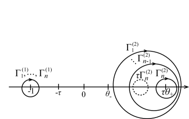
Figure 1: Integration contours in the complex plane. The contour of each $z_{i}$ consists of two curves $\Gamma_{i}^{(1)}$ and $\Gamma_{i}^{(2)}$: the $\Gamma_{i}^{(1)}$’s encircle only the pole -1 and no other pole, and are not nested. The $\Gamma_{i}^{(2)}$’s encircle $\tau\theta_{+}$ with a nesting condition (see text) and exclude the poles at $-1,-\tau$ and $\theta_{-}$.

Remark. By the Cauchy theorem, one can switch to another set of contours s.t. the contour of $z_{i}$ includes $-\tau,\theta_{-}$ and $\{z_{j}/\tau\}_{j<i}$ but not $-1,\tau\theta_{+}$. The contours are now in the counter-clockwise direction and the integrations are performed in the order from $z_{1}$ to $z_{n}$. For the special case with $\theta_{-}=0$, this nesting condition is equivalent to $z_{i}$ not including $\{\tau z_{j}\}_{j>i}$, as employed in [7].

Proof. The integral formula (2.8) (or equivalently, (2.18)) can be proved by showing that the r.h.s. satisfies the Kolmogorov forward equation (or the master equation) for the $n$-particle ASEP together with the initial condition. The fact that (2.8) satisfies the master equation can be checked by using the following relations,

$$\gamma(z)=p\frac{1+z/\tau}{1+z}+q\frac{1+z}{1+z/\tau}-(p+q),$$ (2.12)

$$q\frac{(1+z_{1})(1+z_{2})}{(1+z_{1}/\tau)(1+z_{2}/\tau)}+p-\frac{1+z_{2}}{1+z_{2}/\tau}=\frac{(p-q)(z_{1}-\tau z_{2})}{(1+z_{1}/\tau)(1+z_{2}/\tau)}.$$ (2.13)

When particles are far apart, the first relation suffices. The second formula is used to deal with the special case when two particles are on neighboring sites. For example, for $n=2$, the factor $z_{1}-\tau z_{2}$ cancels the pole at $z_{1}=\tau z_{2}$; the integrand becomes antisymmetric and the integral vanishes.

For verifying the initial condition, one first observes that when $t=0$ the essential singularities at $z_{i}=-1,-\tau$ are absent and one can evaluate the contour integrals explicitly by taking either the pole at -1 or at $-\tau$ depending on whether $x_{i}$ is positive or negative and taking the pole at around $\tau\theta_{+}$ or $\theta_{-}$. For example, for $n=1$ we get

$$\langle\tau^{N(x,0)}\rangle=\begin{cases}(1-\rho_{+}+\tau\rho_{+})^{x},&x\geq 0,\\ (1-\rho_{-}+\frac{\rho_{-}}{\tau})^{-x},&x\leq 0,\end{cases}$$ (2.14)

and for $n=2$,

$$\langle\tau^{N(x_{1},0)+N(x_{2},0)}\rangle=\begin{cases}(1-\rho_{+}+\tau^{2}\rho_{+})^{x_{1}}(1-\rho_{+}+\tau\rho_{+})^{x_{2}-x_{1}},&1\leq x_{1}<x_{2},\\ (1-\rho_{-}+\frac{\rho_{-}}{\tau})^{-x_{1}}(1-\rho_{+}+\tau\rho_{+})^{x_{2}},&x_{1}\leq 0<x_{2},\\ (1-\rho_{-}+\frac{\rho_{-}}{\tau})^{-x_{1}+x_{2}}(1-\rho_{-}+\frac{\rho_{-}}{\tau^{2}})^{-x_{2}},&x_{1}<x_{2}<0.\end{cases}$$ (2.15)

For general $n$, for the case in which $x_{1}<\ldots<x_{l-1}\leq 0<x_{l}<\ldots x_{n},1\leq l\leq n$,

$$\langle\prod_{i=1}^{n}\tau^{N(x_{i},0)}\rangle =\prod_{i=1}^{l-2}(1-\rho_{-}+\rho_{-}/\tau^{i})^{x_{i+1}-x_{i}}(1-\rho_{-}+\rho_{-}/\tau^{l-1})^{-x_{l-1}}$$

$$\quad\times(1-\rho_{+}+\tau^{n-l+1})^{x_{l}}\prod_{i=l}^{n-1}(1-\rho_{+}+\tau^{n-i}\rho_{+})^{x_{i+1}-x_{i}}.$$ (2.16)

They are the correct initial conditions because we are considering the Bernoulli measure with parameters $\rho_{\pm}$ to the right and left.

Finally proposition 2.2 ensures that (2.8) is a representation of the $\tau$-correlation for ASEP with the two-sided Bernoulli initial condition. ∎

We emphasize that the above integral formula for the $\tau$-correlation is valid for arbitrary $\tau<1$. When taking the symmetric limit, $\tau\to 1$, it is useful to rewrite it using the change of variables,

$$\xi_{i}=\frac{1+z_{i}}{1+z_{i}/\tau}.$$ (2.17)

Then the formula (2.8) can be rewritten as

$$\langle\prod_{i=1}^{n}\tau^{N(x_{i},t)}\rangle =(1-\tau)^{n}\left(r_{+}-\frac{r_{-}}{\tau^{i}}\right)\tau^{n(n-1)/2}\int\cdots\int\prod_{1\leq i<j\leq n}\frac{\xi_{i}-\xi_{j}}{\tau-(1+\tau)\xi_{j}+\xi_{i}\xi_{j}}$$

$$\quad\times\prod_{i=1}^{n}e^{\varepsilon_{p,q}(\xi_{i})t}\xi_{i}^{x_{i}}\prod_{i=1}^{n}\frac{1}{(1-\xi_{i}-(1-\tau)\rho_{+})(1-\xi_{i}+(1-1/\tau)\rho_{-}\xi_{i})}d\xi_{i}$$ (2.18)

where $\varepsilon_{p,q,}(\xi)=p\xi+q/\xi-(p+q)$ and the contours are obtained from those for the $z_{i}$ variables; they are around $0,1-(1-\tau)\rho_{+}$ with some nesting conditions. Note in the symmetric limit with $p=q=1$, $\varepsilon_{p,q}$ tends to $\xi+1/\xi-2=\varepsilon(\xi)$ as defined in Theorem 1.1.

2.3 Contour integral formula for the $n$-th moment

The formula (2.8) for the $\tau$-correlation has been obtained and proved to be valid only for $x_{1}<\cdots<x_{n}$. In order to obtain an expression for the $\tau$-moment of order $n$ for $N(x,t)$ at a given point $x$, we would need to take $x_{i}\equiv x$ in (2.8). At this stage of our discussions, there is absolutely no guarantee that by setting $x_{i}\equiv x$ we would obtain a valid and meaningful representation for the $\tau$-moment of order $n$. But, in fact, it turns out that the resulting expression is the correct one.

Proposition 2.4.

For $n\in\mathbb{Z}$, the $n$-th $\tau$-moment of $N(x,t)$ is given by

$$\langle\tau^{nN(x,t)}\rangle=\prod_{i=1}^{n}\left(1-\frac{r_{-}}{\tau^{i}r_{+}}\right)\tau^{n(n-1)/2}\int\cdots\int\prod_{i<j}\frac{z_{i}-z_{j}}{z_{i}-\tau z_{j}}\prod_{i=1}^{n}F_{x,t}(z_{i})dz_{i}.$$ (2.19)

The function $F_{x,t}(z)$ and the contours of $z_{i}$ are the same as in Proposition 2.3.

This issue of finding $\tau$-moment formula from $\tau$-correlation was already noted in [21, 7] where the case with only a finite number of particles on the left side was treated. There another duality function was introduced and it was shown that the $\tau$-moment can be written as a sum of the correlation functions of this modified quantity evaluated at different points. However, the arguments developed in [21, 7] are specific for the case with only a finite number of particles to the left of the origin; these arguments do not work for our case with finite densities on the both sides.

Here we give a different approach. We will write down the time evolution equation of the $\tau$-moment and show that the above formula satisfies that equation. To do so we need to write down the evolution equation for a more general case than the one covered by duality, Proposition 2.1. Suppose that $x_{j},j=1,\ldots,n$ are grouped into the form $(y_{i},m_{i}),1\leq i\leq k$ with multiplicity $m_{i}$, i.e., $x_{j}=y_{i}$ for $\sum_{l=1}^{i-1}m_{l}<j\leq\sum_{l=1}^{i}m_{l},1\leq i\leq k$.

Proposition 2.5.

The time evolution equation for the $n$-th moment is given by

$$\quad\frac{d}{dt}\langle\tau^{nN(x,t)}\rangle=$$

$$\Big{\langle}\tau^{(n-2)N(x,t)}\left(a_{n}\tau^{2N(x,t)}+b_{n}\tau^{N(x,t)+N(x-1,t)}+c_{n}\tau^{N(x,t)+N(x+1,t)}+d_{n}\tau^{N(x+1,t)+N(x-1,t)}\right)\Big{\rangle}$$ (2.20)

with

$$a_{n}=\frac{q(1-\tau^{-n})(-\tau^{3}+\tau^{n})}{(1-\tau)^{2}},\quad b_{n}=\frac{p(1-\tau^{-n})(\tau^{2}-\tau^{n})}{(1-\tau)^{2}},$$ (2.21)

$$c_{n}=\frac{q(1-\tau^{-n})(\tau^{2}-\tau^{n})}{(1-\tau)^{2}},\quad d_{n}=\frac{p(1-\tau^{-n})(-\tau+\tau^{n})}{(1-\tau)^{2}}.$$ (2.22)

Denote the rhs of (2.20) by $V_{n}(x,t)$. For the general case with $(y_{i},m_{i})$’s, the evolution equation is given as a linear combination for the $m_{i}$-th moments at $y_{i}$, namely,

$$\frac{d}{dt}\langle\prod_{i=1}^{k}\tau^{\sum_{i}m_{i}N(y_{i},t)}\rangle=\sum_{i=1}^{k}V_{m_{j}}(y_{j},t).$$ (2.23)

Note that the evolution equation for the moment (2.20) can be seen as a linear equation with inhomogeneous term given by the (lower-order) $\tau$-correlations. If one can find quantities which satisfy both (2.23) and (2.20), they will give the formulas for $\tau$-correlations with $x_{1}\leq\cdots\leq x_{N}$ including $\tau$-moments.

To prove the proposition, the following simple identity will be useful.

$$\tau\tau^{2N(x-1,t)}+\tau^{2N(x,t)}-(1+\tau)\tau^{N(x-1,t)+N(x,t)}=0,$$ (2.24)

which is equivalent to $(\tau^{\eta_{x}}-\tau)\eta_{x}=0$ and can be checked easily by observing that the left hand side vanishes irrespective of the value of the particle occupation at $x$ being $\eta_{x}=0$ or 1.

Proof of Proposition 2.5. First we prove (2.20) by a stochastic calculus similar to that in subsection 2.2. Considering the change of $\tau^{nN(x,t)}$ during the infinitesimal time duration $dt$, we find

$$\tau^{ndN(x,t)}-1=\begin{cases}\tau^{n}-1,&\text{with rate}\quad q\eta_{x+1}(t)(1-\eta_{x}(t)),\\ 1/\tau^{n}-1,&\text{with rate}\quad p\eta_{x}(t)(1-\eta_{x+1}(t)),\\ 0,&\text{otherwise}.\end{cases}$$ (2.25)

Because $\eta_{x}$ and $\eta_{x+1}$ are binary variables, there are some coefficients $a_{n},b_{n},c_{n},d_{n}$ such that the following holds.

$$q(\tau^{n}-1)\eta_{x+1}(1-\eta_{x})+p(1/\tau^{n}-1)\eta_{x}(1-\eta_{x+1})=a_{n}+b_{n}\tau^{-\eta_{x}}+c_{n}\tau^{\eta_{x+1}}+d_{n}\tau^{\eta_{x+1}-\eta_{x}}.$$ (2.26)

One can readily check that they are exactly given by (2.22). Then (2.20) follows immediately.

Next we consider the general case. When $\{x_{i}\}$’s consist of several separate clusters ($y_{i+1}-y_{i}>1$ for some $i$), it is obvious that the time evolution equation is a linear combination of those for each cluster. Hence in the following we consider the case of a single cluster, i.e., $y_{i+1}-y_{i}=1,\forall i$. Then the shape of the cluster is determined by a list $(m_{1},\cdots,m_{k})$ with $\sum_{j=1}^{k}m_{j}=n$. For example, when $N=4$, there are eight possible lists, 1111, 211, 121, 112, 22, 31, 13, 4. We now order them. On lists corresponding to different partitions (1111, 211, 22, 31, 4 for $n=4$), we put the lexicographic ordering ($1111<211<22<31<4$). For lists which share the same partition, we put the order by the value of $\sum_{j=1}^{k}jm_{j}$, e.g., $211<121<112$. When these values are the same, we don’t specify the order between them. For example 312 and 231 have the same values.

Then our basic strategy of proof is to use recursions with respect to this ordering by applying (2.24) by writing it as $\tau^{2N(x,t)}=(1+\tau)\tau^{N(x-1,t)+N(x,t)}-\tau\tau^{2N(x-1,t)}$. For a given $(m_{1},\cdots,m_{k})$’s, find $\text{max}~{}m_{i}$ and take the smallest $j$ s.t. $m_{j}=\text{max}~{}m_{i}$. If $m_{j-1}\leq m_{j}-2$, we apply (2.24) with $x=y_{j}$ and rewrite $\langle\prod_{i=1}^{k}\tau^{\sum_{i}m_{i}N(y_{i},t)}\rangle$ as the sum of two terms with strictly lower order. For example $224$ can be rewritten as a sum of $233$ and $242$. If $\max(1,m_{j-l-1})<m_{j-k}=m_{j}-1,k=1,\ldots,l,1\leq l<j$, where $l$ is the number of $m$’s having the same value $m_{j}$, one applies (2.24) with $x=y_{j-l}$. For example $334$ is rewritten as a sum of $1234$ and $2134$. The remaining case is when $m_{i}=1,1\leq i\leq j-1,m_{j}=2$. When $j\neq k$, we apply (2.24) with $x=y_{j}$ and when $j=k$, we apply (2.24) by writing it as $\tau^{2N(x-1,t)}=(1+\tau^{-1})\tau^{N(x-1,t)+N(x,t)}-\tau^{-1}\tau^{2N(x,t)}$. Anyway we can rewrite $\langle\prod_{i=1}^{k}\tau^{\sum_{i}m_{i}N(y_{i},t)}\rangle$ as the sum of two terms with lower order. We can conclude our proof by recalling that $m_{i}=1,1\leq i\leq k$ case is trivial because this corresponds to a $\tau$-correlation for which the time evolution equation was derived in the previous subsection. ∎

Proof of Proposition 2.4. From the formulas, it is clear that the expression (2.8) for $\tau$-correlations and moments with $x_{1}\leq\cdots\leq x_{N}$ (including (2.19) as a special case) is consistent with (2.24). Using the same rewriting as in the proof of Proposition 2.5 and recursions, one sees that (2.8), (2.19) satisfy (2.23). Then from the discussions below (2.23), it is automatically guaranteed that the formula (2.19) gives the correct formula for the $\tau$-moment. ∎

Remark. The evolution equation for the moments (2.20) in Proposition 2.4 for $n\geq 3$ can also be derived by applying (2.24) and using induction. This alternative proof will be explained in Appendix C.

Remark. Recently, there appeared a work on the stationary ASEP [1], in which ASEP is treated as a special case of the higher spin vertex model. In such higher spin vertex models, more than one particle can occupy the same site. Then, one can readily set $x_{i}=x,\forall i$ in the correlation found in [1] to get a formula for the moment. (See also [8].)

2.4 Residue expansion of the contour integral

Before considering the symmetric limit, it is useful to perform an expansion of (2.19) in terms of residues. Using the definition of the contours in Proposition 2.3, we write (2.19) as the sum of $2^{n}$ terms. Each term is an integral with $k$ contours around $-1$ and $n-k$ nested contours around $\tau\theta_{+}$, and is indexed by a subset $P(\subset\{1,\ldots,n\})$ of cardinality $|P|=k$, corresponding to the contours around $-1$. Evaluating the residues at poles related to $\rho_{+}$ (which are at $\tau^{i}\theta_{+},i\in\mathbb{Z}$) from $z_{n}$ to $z_{1}$, we obtain the following expansion,

$$\langle\tau^{nN(x,t)}\rangle =\sum_{k=0}^{n}(-1)^{k}\prod_{i=1}^{n-k}e^{\Lambda_{i}}\prod_{i=n-k+1}^{n}\left(1-\frac{r_{-}}{\tau^{i}r_{+}}\right)$$

$$\quad\times\sum_{\begin{subarray}{c}P\subset\{1,\ldots,n\}\\ |P|=k\end{subarray}}\tau^{v(P)}\int_{-1}\cdots\int_{-1}f_{P}(z_{1},\ldots,z_{k})\prod_{i=1}^{k}dz_{i},$$ (2.27)

where $v(P)=||P||-k$ with $||P||=\sum_{i\in P}i$, and where $\Lambda_{i}=\Lambda_{i}(x,t)$ is defined by

$$e^{\Lambda_{i}}=\left(\frac{1+\tau^{i}\theta_{+}}{1+\tau^{i-1}\theta_{+}}\right)^{x}e^{\varepsilon(\tau^{i}\theta_{+})t}.$$ (2.28)

Notice that because of the order of evaluation of the residues there are no contributions from the poles coming from $1/(z_{i}-\tau z_{j})$. When the pole related to $\rho_{+}$ is taken for $z_{j}$, the denominator in $F_{x,t}$ is canceled by the numerator in the factor $(z_{i}-z_{j})/(z_{i}-\tau z_{j})$ and is replaced by its denominator. This procedure gives an extra factor of $\tau^{j-1}$, which leads to the overall $\tau$ factor with the exponent $n(n-1)/2-\sum_{j\neq P}(j-1)=\sum_{i\in P}(i-1)=v(P)$. The function $f_{P}$ depends also on $P$ but the dependence will become irrelevant in the symmetric limit which is our main interest, see (3.4).

To understand the structure, it would be useful to see a few examples. The above expansion reads, for $n=1$,

$$\langle\tau^{N(x,t)}\rangle=e^{\Lambda_{1}}-(1-\frac{r_{-}}{\tau r_{+}})\int_{-1}F_{x,t}(z)dz$$ (2.29)

and for $n=2$,

$$\langle\tau^{2N(x,t)}\rangle =e^{\Lambda_{1}+\Lambda_{2}}-e^{\Lambda_{1}}(1-\frac{r_{-}}{\tau^{2}r_{+}})\left(\int_{-1}dz_{1}\frac{\left(\frac{1+z_{1}}{1+z_{1}/\tau}\right)^{x_{1}}e^{\varepsilon(z_{1})t}}{(1-\frac{z_{1}}{\tau^{2}\theta_{+}})(z_{1}-\theta_{-})}+\tau\int_{-1}dz_{2}\frac{\left(\frac{1+z_{2}}{1+z_{2}/\tau}\right)^{x_{1}}e^{\varepsilon(z_{2})t}}{(1-\frac{z_{2}}{\theta_{+}})(z_{2}-\theta_{-})}\right)$$

$$\quad+(1-\frac{r_{-}}{\tau r_{+}})(1-\frac{r_{-}}{\tau^{2}r_{+}})\tau\int_{-1}dz_{1}\int_{-1}dz_{2}\frac{z_{1}-z_{2}}{z_{1}-\tau z_{2}}F_{x,t}(z_{1})F_{x,t}(z_{2}).$$ (2.30)

3 The Symmetric Exclusion Process limit

In this section we take the symmetric limit of the results in the previous section and prove our key result in the paper, Proposition 1.2. Let us denote the height for SEP by $N=N(x,t)$ and the height for ASEP by $N_{\text{ASEP}}=N_{\text{ASEP}}(x,t)$ to make a clear distinction. We see, for $\tau=1-\epsilon,\epsilon\to 0$,

$$\tau^{N_{\text{ASEP}}}=1-\epsilon N+O(\epsilon^{2})$$ (3.1)

and hence

$$\langle(1-\tau^{N_{\text{ASEP}}})^{n}\rangle=\epsilon^{n}\langle N^{n}\rangle+o(\epsilon^{n}).$$ (3.2)

In other words, the $n$th moment of SEP can be found by the lowest $n$th order (in $\epsilon$) coefficient from the moments of ASEP with degree $n$ and lowers. In terms of $\tau$-moments for ASEP, the l.h.s. of (3.2) is expanded as

$$\langle(1-\tau^{N_{\text{ASEP}}})^{n}\rangle=\sum_{j=0}^{n}(-1)^{n-j}\binom{n}{j}\langle\tau^{(n-j)N_{\text{ASEP}}}\rangle.$$ (3.3)

In the $\tau$-deformed moment formula for ASEP (2.27), the integrand in the $k$-fold integral $f_{P}$ depends on $P$ and the formula is fairly involved. But applying the change of variable (2.17) in the pole expansion formula (2.27), and taking the limit, $\epsilon=1-\tau\downarrow 0$, one observes that it depends only on $k$ to the leading order as follows,

$$\int_{-1}\cdots\int_{-1}f_{P}(z_{1},\ldots,z_{k})\prod_{i=1}^{k}dz_{i}=\epsilon^{k}r_{+}^{k}J_{k}+O(\epsilon^{k+1})$$ (3.4)

where $J_{k}$ was defined in (1.33). To understand the appearance of the common $J_{k}$, it may be useful to look at a specific case: for example, the integrands of the $z_{1}$ integrals in the second term on the right hand side of (2.30) are different but become the same in the $\tau\to 1$ limit. The factor $\epsilon^{k}r_{+}^{k}$ is due to the change of variable (2.17) as in the transformation from (2.8) to (2.18).

Substituting (3.4) in (2.27), we obtain

$$\langle\tau^{nN_{\text{ASEP}}}\rangle =\sum_{k=0}^{n}\epsilon^{k}\prod_{i=1}^{n-k}e^{\Lambda_{i}}\prod_{i=n-k+1}^{n}\left(r_{+}-\frac{r_{-}}{\tau^{i}}\right){n\brack k}_{\tau}(-1)^{k}\tau^{k(k-1)/2}(J_{k}+O(\epsilon))$$ (3.5)

where we used $\sum_{P\subset\{1,2,\cdots,n\},|P|=k}\tau^{||P||-k}={n\brack k}_{\tau}\tau^{k(k-1)/2}$ (which is proved by multiplying by $x^{k}$ and taking a sum $\sum_{k=0}^{n}$ to get a $q$-binomial theorem $\prod_{k=0}^{n-1}(1+x\tau^{k})=\sum_{k=0}^{n}{n\brack k}_{\tau}\tau^{k(k-1)/2}x^{k}.$) Hence

$$\quad\langle(1-\tau^{N_{\text{ASEP}}})^{n}\rangle=\sum_{j=0}^{n}\binom{n}{j}(-1)^{j}\langle\tau^{jN_{\text{ASEP}}}\rangle$$

$$=\sum_{j=0}^{n}\binom{n}{j}(-1)^{j}\sum_{k=0}^{j}\epsilon^{k}{j\brack k}_{\tau}\prod_{i=1}^{j-k}e^{\Lambda_{i}}\prod_{i=j-k+1}^{j}\left(r_{+}-\frac{r_{-}}{\tau^{i}}\right)(-1)^{k}\tau^{k(k-1)/2}(J_{k}+O(\epsilon))$$

$$=\sum_{k=0}^{n}\left\{\sum_{j=k}^{n}(-1)^{j-k}\binom{n}{j}{j\brack k}_{\tau}\prod_{i=1}^{j-k}e^{\Lambda_{i}}\prod_{i=j-k+1}^{j}\left(r_{+}-\frac{r_{-}}{\tau^{i}}\right)\right\}\tau^{k(k-1)/2}\epsilon^{k}(J_{k}+O(\epsilon)).$$ (3.6)

Let us define

$$\mu_{n,k}(\epsilon)=\sum_{j=k}^{n}(-1)^{j-k}\binom{n}{j}{j\brack k}_{\tau}\prod_{i=1}^{j-k}e^{\Lambda_{i}}\prod_{i=j-k+1}^{j}\left(r_{+}-\frac{r_{-}}{\tau^{i}}\right).$$ (3.7)

We will show that the following limit exists:

$$\tilde{m}_{n,k}=\lim_{\epsilon\to 0}\mu_{n,k}(\epsilon)/\epsilon^{n-k},$$ (3.8)

and, therefore, $\mu_{n,k}(\epsilon)=(\tilde{m}_{n,k}+O(\epsilon))\epsilon^{n-k}$. Hence, we can neglect $O(\epsilon)$ in (3.7) so that we obtain

$$\langle N^{n}\rangle=\sum_{k=0}^{n}\tilde{m}_{n,k}J_{k}.$$ (3.9)

Comparing with (1.34), it remains to show that

$$\tilde{m}_{n,k}=m_{n,k}.$$ (3.10)

Let us introduce generating functions of $\mu_{n,k}(\epsilon)$ and $m_{n,k}$ for a fixed $k=0,1,\ldots,n$ as

$$W_{k}(\lambda) =\sum_{n=0}^{\infty}\frac{(\lambda/\epsilon)^{n}}{n!}\mu_{n,k}(\epsilon),$$ (3.11)

$$M_{k}(\lambda) =\sum_{n=0}^{\infty}\frac{\lambda^{n}}{n!}\tilde{m}_{n,k}.$$ (3.12)

The statements (3.8) and (3.10) are proved by the following proposition:

Proposition 3.1.

$$M_{k}(\lambda)=\lim_{\epsilon\to 0}\epsilon^{k}W_{k}(\lambda)=\frac{\omega^{k}}{k!}(1+\rho_{+}(e^{\lambda}-1))^{x}.$$ (3.13)

Proof. From equation (3.8) for $k=0$, we obtain

$$W_{0}(\lambda)=e^{\lambda/\epsilon}\sum_{n=0}^{\infty}\frac{(-\lambda/\epsilon)^{n}}{n!}\prod_{i=1}^{n}e^{\Lambda_{i}}.$$ (3.14)

Here $\Lambda_{i}$ is given by (2.28). First let us consider the $t=0$ case, for which this expression can be transformed as follows

$$\quad e^{\lambda/\epsilon}\sum_{n=0}^{\infty}\frac{(-\lambda/\epsilon)^{n}}{n!}\left(\frac{1+\tau^{n}\theta_{+}}{1+\theta_{+}}\right)^{x}$$

$$=e^{\lambda/\epsilon}\left(\frac{1}{(1+\theta_{+})^{x}}\sum_{n=0}^{\infty}\frac{(-\lambda/\epsilon)^{n}}{n!}\sum_{m=0}^{x}\binom{x}{m}(\tau^{n}\theta_{+})^{m}\right)$$

$$=\frac{1}{(1+\theta_{+})^{x}}\sum_{m=0}^{x}\binom{x}{m}\theta_{+}^{m}e^{-(\tau^{m}-1)\lambda/\epsilon}.$$ (3.15)

Using $e^{-(\tau^{m}-1)\lambda/\epsilon}\to e^{m\lambda}$ as $\epsilon\to 0$, we conclude from (3.15) that $W_{0}(\lambda)$ converges to $M_{0}(\lambda)=(1+\rho_{+}(e^{\lambda}-1))^{x}$ in the small $\epsilon$ limit.

When $t>0$, (3.15) should be multiplied by $e^{\sum_{i=1}^{n}\epsilon(\tau^{i}\theta_{+})t}$. We will argue that this factor does not change $\lim_{\epsilon\to 0}W_{0}(\lambda)$. First we rewrite $\gamma(z)$ in (2.11) as $\gamma(z)=q(1-\tau)(1/(1+z/\tau)-1/(1+z))$ and find

$$e^{\sum_{i=1}^{n}\gamma(\tau^{i}\theta_{+})t}=e^{\frac{q(1-\tau)}{1+\theta_{+}}t}e^{-\frac{q(1-\tau)}{1+\tau^{n}\theta_{+}}t}=e^{\frac{q\epsilon}{1+\theta_{+}}t}\times\sum_{j=0}^{\infty}\frac{(qt)^{j}}{j!(1+\tau^{n}\theta_{+})^{j}}\epsilon^{j}.$$ (3.16)

The first factor $e^{\frac{q\epsilon}{1+\theta_{+}}t}$ is independent of $n$ and tends to unity in the $\epsilon\to 0$ limit so that obviously it does not influence the limit $\lim_{\epsilon\to 0}W_{0}(\lambda)$. For the second factor, the $j$th term cancels the factor $(1+\tau^{n}\theta_{+})^{x}$ in the leftmost side of (3.15) and hence we have

$$\quad e^{\lambda/\epsilon}\sum_{n=0}^{\infty}\frac{(-\lambda/\epsilon)^{n}}{n!}\left(\frac{1+\tau^{n}\theta_{+}}{1+\theta_{+}}\right)^{x}e^{-\frac{q(1-\tau)}{1+\tau^{n}\theta_{+}}t}$$

$$=\sum_{j=0}^{\infty}\frac{1}{j!}\left(\frac{qt}{1+\theta_{+}}\right)^{j}\left(\frac{1}{1+\rho_{+}(e^{\lambda}-1)}\right)^{j}\epsilon^{j}\times M_{0}(\lambda)|_{t=0}$$

$$=\exp\left(\frac{qt}{(1+\tau^{n}\theta_{+})(1+\rho_{+}(e^{\lambda}-1))}\epsilon\right)M_{0}(\lambda)|_{t=0}.$$ (3.17)

Here in the first equality we used (3.15). With this expression it is easy to see that, when $\epsilon\to 0$, we have $\lim_{\epsilon\to 0}W_{0}(\lambda)=M_{0}(\lambda)$ for all $t\geq 0$.

Using similar calculations for $k>0$ we obtain

$$\epsilon^{k}W_{k}(\lambda) =e^{\lambda/\epsilon}\frac{\lambda^{k}}{[k]_{\tau}!}\sum_{l=0}^{\infty}(-1)^{l}\frac{[l+k]_{\tau}!(\lambda/\epsilon)^{l}}{[l]_{\tau}!(l+k)!}\prod_{i=l+1}^{l+k}(r_{+}-r_{-}/\tau^{i})\prod_{p=1}^{l}e^{\Lambda_{p}}$$

$$=e^{\lambda/\epsilon}\frac{\epsilon^{k}}{[k]_{\tau}!}\sum_{l=0}^{\infty}\frac{[l]_{\tau}!(-\lambda/\epsilon)^{l}}{[l-k]_{\tau}!l!}\prod_{i=l-k+1}^{l}(r_{+}-r_{-}/\tau^{i})\prod_{p=1}^{l-k}e^{\Lambda_{p}}.$$ (3.18)

Note that in the middle expression the sum over $l$ can be made starting from $-k$ due to the factor $[l+k]_{\tau}!/[l]_{\tau}!$. Accordingly we made a shift $l\to l-k$ in the second equality.

Expanding the two factors $[l+k]_{\tau}!/[l]_{\tau}!=\prod_{i=0}^{k-1}(1-\tau^{l-i})$ and $\prod_{i=l-k+1}^{l}(r_{+}-r_{-}/\tau^{i})$, one can perform the sum over $l$ and do similar calculations as for the $k=0$ case above. Observing that an extra factor $\tau^{i}$ in front of $\tau^{l}$ would not make any difference in the $\epsilon\to 0$ limit, we can now replace the factor $[l+k]_{\tau}!/[l]_{\tau}!$ by $(1-\tau)^{l}$, $\prod_{i=l-k+1}^{l}(r_{+}-r_{-}/\tau^{i})$ by $(r_{+}-r_{-}/\tau^{l})^{k}$ and $\prod_{i=1}^{l-k}e^{\Lambda_{i}}$ by $\prod_{i=1}^{l}e^{\Lambda_{i}}$ with errors of $O(\epsilon)$ in the final result. Therefore expanding the first two factors with binomial coefficients we find

$$\epsilon^{k}W_{k}(\lambda) =\frac{e^{\lambda/\epsilon}}{k!}\sum_{j=0}^{k}(-1)^{j}\binom{k}{j}\sum_{i=0}^{k}\binom{k}{i}r_{+}^{k-i}r_{-}^{i}\sum_{l=0}^{\infty}(-1)^{l}\frac{(\lambda/\epsilon)^{l}}{l!}\tau^{(j-i)l}\prod_{p=1}^{l}e^{\Lambda_{p}}+O(\epsilon).$$ (3.19)

When $t=0$ one applies the same calculation as in (3.15) to find

$$e^{\lambda/\epsilon}\sum_{l=0}^{\infty}(-1)^{l}\frac{(\lambda/\epsilon)^{l}}{l!}\tau^{(j-i)l}\prod_{p=1}^{l}e^{\Lambda_{p}}=\frac{1}{(1+\theta_{+})^{x}}\sum_{m=0}^{x}\binom{x}{m}\theta_{+}^{m}e^{-(\tau^{m+j-i}-1)\lambda/\epsilon}\xrightarrow{\epsilon\to 0}e^{(j-i)\lambda}W_{0}(\lambda).$$ (3.20)

One can also check that $t>0$ would not change the limit as in the $k=0$ case. Observing

$$\sum_{j=0}^{k}(-1)^{j}\binom{k}{j}\sum_{i=0}^{k}\binom{k}{i}r_{+}^{k-i}r_{-}^{i}e^{(j-i)\lambda}=(e^{\lambda}-1)^{k}(r_{+}+r_{-}e^{-\lambda})^{k}=\omega^{k},$$ (3.21)

we finally arrive at (3.13).

Comparing (3.13) with (1.32), one finds $\tilde{m}_{n,k}=m_{n,k}$, concluding the proof of Proposition 3.1. ∎

4 Fredholm determinant for the integrals $J_{n}$

In this section we prove Proposition 1.3 by adapting the arguments in, for example, [45, 14]. Let us first recall

$$J_{n} =\int_{C_{0}}\cdots\int_{C_{0}}\prod_{1\leq i<j\leq n}\frac{\xi_{i}-\xi_{j}}{\xi_{i}\xi_{j}+1-2\xi_{j}}\prod_{i=1}^{n}\frac{\xi_{i}^{x}e^{\varepsilon(\xi_{i})t}d\xi_{i}}{(1-\xi_{i})^{2}}$$ (4.1)

where $C_{0}$ is a contour around the origin with radius so small that the poles from the factor $1/(\xi_{i}\xi_{j}+1-2\xi_{j})$ in the integrand are not included. We rewrite $J_{n}$ as

$$J_{n} =\int_{C_{0}}\cdots\int_{C_{0}}\prod_{1\leq i\neq j\leq n}\frac{1}{\xi_{i}\xi_{j}+1-2\xi_{j}}\cdot\prod_{1\leq i<j\leq n}(\xi_{i}\xi_{j}+1-2\xi_{i})\prod_{1\leq i<j\leq n}(\xi_{i}-\xi_{j})\cdot\prod_{i=1}^{n}\frac{\xi_{i}^{x}e^{\varepsilon(\xi_{i})t}d\xi_{i}}{(1-\xi_{i})^{2}}.$$ (4.2)

We can relabel the indices by $i$ by an arbitrary permutation ${\sigma\in S_{n}}$, where $S_{n}$ is the permutation group $(1,2,\cdots,n)$. Taking into account that the products over all ${1\leq i\neq j\leq n}$ are permutation-symmetric and the Vandermonde product is antisymmetric, the above integral can be rewritten as

$$\int_{C_{0}}\cdots\int_{C_{0}}\prod_{1\leq i\neq j\leq n}\frac{1}{\xi_{i}\xi_{j}+1-2\xi_{j}}\cdot{\rm{sgn}}\sigma\prod_{1\leq i<j\leq n}(\xi_{\sigma(i)}\xi_{\sigma(j)}+1-2\xi_{\sigma(i)})$$

$$\times\prod_{1\leq i<j\leq n}(\xi_{i}-\xi_{j})\prod_{i=1}^{n}\frac{\xi_{i}^{x}e^{\varepsilon(\xi_{i})t}d\xi_{i}}{(1-\xi_{i})^{2}}$$

Summing over all permutations $\sigma$ in the set $S_{n}$ (and normalizing by $1/n!$), we have

$$J_{n} =\int_{C_{0}}\cdots\int_{C_{0}}\prod_{1\leq i\neq j\leq n}\frac{1}{\xi_{i}\xi_{j}+1-2\xi_{j}}\cdot\prod_{1\leq i<j\leq n}(\xi_{i}-\xi_{j})\cdot\prod_{i=1}^{n}\frac{\xi_{i}^{x}e^{\varepsilon(\xi_{i})t}d\xi_{i}}{(1-\xi_{i})^{2}}$$

$$\hskip 56.9055pt\times\frac{1}{n!}\sum_{\sigma\in S_{n}}{\rm{sgn}}\sigma\prod_{1\leq i<j\leq n}(\xi_{\sigma(i)}\xi_{\sigma(j)}+1-2\xi_{\sigma(i)})$$

$$=\int_{C_{0}}\cdots\int_{C_{0}}\prod_{1\leq i\neq j\leq n}\frac{\xi_{i}-\xi_{j}}{\xi_{i}\xi_{j}+1-2\xi_{j}}\cdot\prod_{1\leq i<j\leq n}(\xi_{i}-\xi_{j})\cdot\prod_{i=1}^{n}\frac{\xi_{i}^{x}e^{\varepsilon(\xi_{i})t}d\xi_{i}}{(1-\xi_{i})^{2}}$$

$$=\int_{C_{0}}\cdots\int_{C_{0}}\det(K_{x,t}(\xi_{i},\xi_{j}))_{i,j=1}^{n}\prod_{i=1}^{n}d\xi_{i},$$ (4.3)

where

$$K_{x,t}(\xi_{1},\xi_{2})=\frac{\xi_{1}^{x}e^{\varepsilon(\xi_{1})t}}{\xi_{1}\xi_{2}+1-2\xi_{2}}$$ (4.4)

is the kernel that appears in Theorem 1.1. The equation (4.3) says that $J_{n}$ is the $n$th term in the Fredholm expansion of the Fredholm determinant given in (1.34).

In the derivation of (4.3), we use the following two combinatorial identities,

$$\sum_{\sigma\in S_{n}}{\rm{sgn}}\sigma\prod_{1\leq i<j\leq n}(\xi_{\sigma(i)}\xi_{\sigma(j)}+1-2\xi_{\sigma(i)})=n!\prod_{1\leq i<j\leq n}(\xi_{j}-\xi_{i}),$$ (4.5)

$$\prod_{k=1}^{n}\frac{1}{(1-\xi_{k})^{2}}\prod_{i\neq j}\frac{\xi_{i}-\xi_{j}}{\xi_{i}\xi_{j}+1-2\xi_{j}}=\det\left(\frac{1}{\xi_{i}\xi_{j}+1-2\xi_{i}}\right)_{i,j=1,\cdots,n}.$$ (4.6)

The last equation has been proved in [45]. The identity (4.5) can be shown as follows: Changing the variable as $t_{i}=1/(\xi_{i}-1)$, (4.5) becomes

$$\sum_{\sigma\in S_{n}}{\rm{sgn}}\sigma\prod_{1\leq i<j\leq n}(1+t_{\sigma(i)}-t_{\sigma(j)})=n!\prod_{1\leq i<j\leq n}(t_{i}-t_{j}).$$ (4.7)

We introduce an arbitrary parameter $a\in\mathbb{C}$ and prove a slightly more general formula,

$$\sum_{\sigma\in S_{n}}{\rm{sgn}}\sigma\prod_{1\leq i<j\leq n}(a+t_{\sigma(i)}-t_{\sigma(j)})=n!\prod_{1\leq i<j\leq n}(t_{i}-t_{j}).$$ (4.8)

Expanding the left hand side with respect to $a$, we observe that the coefficient of $a^{k}$ will be a linear combination of terms of the form

$$\sum_{\sigma\in S_{n}}{\rm{sgn}}\sigma\,t_{\sigma(1)}^{m_{1}}t_{\sigma(2)}^{m_{2}}\cdots t_{\sigma(n)}^{m_{n}}$$ (4.9)

where $m_{j}\in\mathbb{Z}_{\geq 0}~{}$, for $j=1,2,\cdots,n$, satisfy the conditions $0\leq m_{j}\leq n-1$ and $~{}\sum_{j=1}^{n}m_{j}=\frac{n(n-1)}{2}-k.$ Then, for $k\geq 1$, at least some pair of $m_{j},~{}j=1,2,\cdots,n$ should have the same value: this implies that (4.9) vanishes. The polynomial (4.8) does not depend on $a$ and we have

$$\sum_{\sigma\in S_{n}}{\rm{sgn}}\sigma\prod_{1\leq i<j\leq n}(a+t_{\sigma(i)}-t_{\sigma(j)})=\sum_{\sigma\in S_{n}}{\rm{sgn}}\sigma\prod_{1\leq i<j\leq n}(t_{\sigma(i)}-t_{\sigma(j)})=n!\prod_{1\leq i<j\leq n}(t_{i}-t_{j}).$$ (4.10)

∎

Appendix A Moments and cumulants

In this appendix, we summarize a few basic formulas about the moments, cumulants and their generating functions, which are useful for discussions in the main text.

For a random variable $X$, the moment is

$$m_{n}=\langle X^{n}\rangle,~{}~{}n\in\mathbb{N}.$$ (A.1)

Note $m_{0}=1$ for any $X$. The moment generating function is defined by

$$M(\lambda)=\sum_{n=0}^{\infty}\frac{\lambda^{n}}{n!}m_{n}.$$ (A.2)

The cumulant generating function $K(\lambda)$ and the cumulant $c_{n}$ are defined through

$$K(\lambda)=\log M(\lambda)=\sum_{n=1}^{\infty}\frac{\lambda^{n}}{n!}c_{n}.$$ (A.3)

By convention we set $c_{0}=0$.

The relations between the moments and cumulants can be written down explicitly. The moment can be written in terms of cumulants as, for $n\in\mathbb{Z}_{+}$,

$$m_{n}=\sum_{\begin{subarray}{c}\nu\vdash n\\ \nu=1^{l_{1}}2^{l_{2}}\cdots\end{subarray}}a_{\nu}^{n}c_{1}^{l_{1}}c_{2}^{l_{2}}\cdots$$ (A.4)

with

$$a_{\nu}^{n}=n!\prod_{j=1}^{n}\frac{1}{l_{j}!}\left(\frac{1}{j!}\right)^{l_{j}}.$$ (A.5)

For example,

$$m_{1} =c_{1},$$ (A.6)

$$m_{2} =c_{1}^{2}+c_{2},$$ (A.7)

$$m_{3} =c_{1}^{3}+3c_{1}c_{2}+c_{3},$$ (A.8)

$$m_{4} =c_{1}^{4}+6c_{1}^{2}c_{2}+3c_{2}^{2}+4c_{1}c_{3}+c_{4},$$ (A.9)

$$m_{5} =c_{1}^{5}+10c_{1}^{3}c_{2}+15c_{1}c_{2}^{2}+10c_{1}^{2}c_{3}+10c_{2}c_{3}+5c_{1}c_{4}+c_{5}.$$ (A.10)

Conversely the cumulant is written in terms of moments as

$$c_{n}=\sum_{\begin{subarray}{c}\nu\vdash n\\ \nu=1^{l_{1}}2^{l_{2}}\cdots\end{subarray}}\tilde{a}_{\nu}^{n}m_{1}^{l_{1}}m_{2}^{l_{2}}\cdots$$ (A.11)

with

$$\tilde{a}_{\nu}^{n}=(-1)^{l-1}(l-1)!a_{\nu}^{n},\quad l=l_{1}+l_{2}+\cdots.$$ (A.12)

The first few examples are given by

$$c_{1} =m_{1},$$ (A.13)

$$c_{2} =m_{2}-m_{1}^{2},$$ (A.14)

$$c_{3} =m_{3}-3m_{1}m_{2}+2m_{1}^{3},$$ (A.15)

$$c_{4} =m_{4}-4m_{3}m_{1}-3m_{2}^{2}+12m_{2}m_{1}^{3}-6m_{1}^{4},$$ (A.16)

$$c_{5} =m_{5}-5m_{4}m_{1}-10m_{3}m_{2}+20m_{3}m_{1}^{2}+30m_{2}^{2}m_{1}-60m_{2}m_{1}^{3}+24m_{1}^{5}.$$ (A.17)

Now let us set

$$\alpha_{n,l}(a,b)=\sum_{\begin{subarray}{c}\nu\vdash n\\ \nu=1^{l_{1}}2^{l_{2}}\cdots\\ l_{1}+l_{2}+\cdots=l\end{subarray}}\frac{n!}{\prod_{j=1}^{n}l_{j}!}\,\prod_{j=1}^{n}\left(\frac{a+(-1)^{j}b}{j!}\right)^{l_{j}}.$$ (A.18)

This is the same formula as the one defined in (1.39). By the general relations between the moments and cumulants explained above, this is useful for example in the description of cumulants when the moments are known.

Example 1. When the moment generating function is $M(\lambda)=1+a(e^{\lambda}-1)$, the moments are $m_{0}=1$ and $m_{n}=a$ for $n\in\mathbb{Z}_{+}$. The cumulant generating function is $K(\lambda)=\log(1+a(e^{\lambda}-1))$ and the cumulants are

$$c_{n} =\sum_{\begin{subarray}{c}\nu\vdash n\\ \nu=1^{l_{1}}2^{l_{2}}\cdots\end{subarray}}\tilde{a}_{\nu}^{n}a^{\sum_{j=1}^{\infty}l_{j}}=\sum_{l=0}^{n}(-1)^{l}(l-1)!\sum_{\begin{subarray}{c}\nu\vdash n\\ \nu=1^{l_{1}}2^{l_{2}}\cdots\\ l_{1}+l_{2}+\cdots=l\end{subarray}}\frac{n!}{\prod_{j=1}^{n}l_{j}!}\,\prod_{j=1}^{n}\left(\frac{a}{j!}\right)^{l_{j}}$$

$$=\sum_{l=0}^{n}(-1)^{l}(l-1)!\alpha_{n,l}(1,0)a^{l}.$$ (A.19)

Example 2. When the moment generating function is $M(\lambda)=1+a(e^{\lambda}-1)+b(e^{-\lambda}-1)$, the momenta are $m_{0}=1$, $m_{n}=a+b$ for $n=2j$ and $m_{n}=a-b$ for $n=2j-1$ with $j\in\mathbb{Z}_{+}$. The cumulant generating function is $K(\lambda)=\log(1+a(e^{\lambda}-1)+b(e^{-\lambda}-1))$ and the cumulants are

$$c_{n}=\sum_{l=0}^{n}(-1)^{l}(l-1)!\alpha_{n,l}(a,b).$$ (A.20)

Appendix B Asymptotics of $I_{n}$

We prove Proposition 1.6. Our arguments are a generalization of those in [14], but we use the steepest decent method, rather than applying saddle point methods in two steps. In the following the symbol $\sim$ means that the ratio of the left and right hand sides goes to unity as $t\to\infty$ as in Proposition 1.6. For $x\geq 0$, the integral (1.37) can be written as

$$I_{n} =\int_{C_{0}}\cdots\int_{C_{0}}\prod_{j=1}^{n}dz_{j}z_{j}^{x}\frac{e^{(z_{j+1}+1/z_{j}-2)t}}{z_{j}z_{j+1}+1-2z_{j}}=\int_{C_{0}}\cdots\int_{C_{0}}\prod_{j=1}^{n}dz_{j}z_{j}^{x}\frac{e^{(z_{j+1}+1/z_{j}-2)t}-1}{z_{j}z_{j+1}+1-2z_{j}}$$

$$=\int_{C_{0}}\cdots\int_{C_{0}}\prod_{j=1}^{n}\frac{dz_{j}}{z_{j}}z_{j}^{x}\int_{0}^{t}dt_{j}e^{(z_{j+1}+1/z_{j}-2)t_{j}}=\int_{0}^{t}\cdots\int_{0}^{t}\prod_{k=1}^{n}dt_{k}\left[\prod_{k=1}^{n}\int_{C_{0}}\frac{dz_{k}}{z_{k}}e^{t_{k-1}z_{k}+\frac{t_{k}}{z_{k}}-2t_{k}}z_{k}^{x}\right]$$

$$=\int_{0}^{1}\cdots\int_{0}^{1}\prod_{k=1}^{n}du_{k}2tu_{k}e^{-2tu_{k}^{2}}\left[\prod_{k=1}^{n}\int_{C_{0}}\frac{dw_{k}}{w_{k}}e^{tu_{k-1}u_{k}(w_{k}+1/w_{k})}w_{k}^{x}\right]\,.$$ (B.1)

where in the first expression we set $z_{n+1}=z_{1}$ and in the second equality we used $x\geq 0$ so that there is no pole at the origin and also the fact that the radius of the contour $C_{0}$ is so small that there is no pole from the denominators of the integrand. In the last equality we changed the variables from $t_{k},z_{k}$ to $u_{k},w_{k}$ by $t_{k}=tu_{k}^{2}$, $z_{k}=w_{k}u_{k}/u_{k-1}$ (with $u_{0}=u_{n}$).

We now perform a steepest descent analysis on this integral. A standard reference for this method is [50] (for a similar concrete example in the case of a one-dimensional integral see [40], section 5). By changing the variables $(u_{1},\ldots,u_{n})\rightarrow(u,v_{1},\ldots,v_{n-1})$ and $(w_{1},\ldots,w_{n})\rightarrow(\theta_{1},\ldots,\theta_{n})$ as follows

$$u=u_{1},\quad\hbox{ and }\quad v_{i} =\sqrt{t}(u_{i+1}-u_{i})\,\,\hbox{ for }\,\,1\leq i\leq n-1$$ (B.2)

$$w_{k} =e^{i\theta_{k}}\,\,\hbox{ for }\,\,1\leq k\leq n$$ (B.3)

the previous integrals becomes

$$I_{n} =2^{n}t^{\frac{n+1}{2}}\int_{0}^{1}udu\left(\prod_{i=1}^{n-1}\int_{-\sqrt{t}u-V_{i-1}}^{\sqrt{t}(1-u)-V_{i-1}}\right)e^{-V_{n-1}^{2}}\prod_{i=1}^{n-1}(u+\frac{V_{i}}{\sqrt{t}})e^{-v_{i}^{2}}dv_{i}$$

$$\quad\times\prod_{i=1}^{n}\int_{-\pi}^{\pi}\frac{d\theta_{i}}{2\pi}e^{2t\sum_{k=1}^{n}(\cos\theta_{k}-1)(u+\frac{V_{k-2}}{\sqrt{t}})(u+\frac{V_{k-1}}{\sqrt{t}})+ix\sum_{k}\theta_{k}}$$ (B.4)

where we use $V_{i}=\sum_{j=1}^{i}v_{j}$ (with $V_{0}=0$ and $V_{-1}=V_{n-1}$). The integrals over the $d\theta_{i}$’s are transformed further by the change of variable

$$y_{k}^{2}=2t(1-\cos\theta_{k})$$ (B.5)

(Note that when $\theta_{k}\in[-\pi,\pi]$ the variable $y_{k}$ runs over $[-2\sqrt{t},2\sqrt{t}]$.) We obtain, recalling that $x=-2\sqrt{t}\xi$,

$$I_{n} =2^{n}t^{\frac{n+1}{2}}\int_{0}^{1}udu\left(\prod_{i=1}^{n-1}\int_{-\sqrt{t}u-V_{i-1}}^{\sqrt{t}(1-u)-V_{i-1}}\right)e^{-(\sum_{i=1}^{n-1}v_{i})^{2}}\prod_{i=1}^{n-1}(u+\frac{V_{i}}{\sqrt{t}})e^{-v_{i}^{2}}dv_{i}$$

$$\quad\times\prod_{i=1}^{n}\left(\int_{-2\sqrt{t}}^{2\sqrt{t}}\frac{dy_{i}}{2\pi\sqrt{t}\sqrt{1-\frac{y_{i}^{2}}{4t}}}e^{-y_{i}^{2}(u+\frac{V_{i-2}}{\sqrt{t}})(u+\frac{V_{i-1}}{\sqrt{t}})-2i\sqrt{t}\xi\arccos(1-\frac{y_{i}^{2}}{2t})}\right)$$ (B.6)

We can now take the limit $t\to\infty$ in this previous integral:

$$I_{n} \sim\sqrt{t}\pi^{-n/2}\int_{0}^{1}u^{n}du\left(\prod_{i=1}^{n-1}\int_{-\infty}^{+\infty}e^{-v_{i}^{2}}dv_{i}\right)e^{-(\sum_{i}v_{i})^{2}} \prod_{i=1}^{n}\left(\int_{-\infty}^{\infty}dy_{i}e^{-y_{i}^{2}u^{2}-2i\xi y_{i}}\right)$$ (B.7)

Evaluating the Gaussian integrals, we conclude that

$$I_{n}\sim\sqrt{\frac{t}{n\pi}}\int_{0}^{1}due^{-\frac{n\xi^{2}}{u^{2}}}=\sqrt{t}\Xi_{n}(|\xi|)=\sqrt{t}\Xi_{n}(-\xi)\,,$$ (B.8)

where the last equality is found by changing the variable $u\to 1/u$ and by using the last expression of $\Xi(\xi)$ in (1.45). This concludes the proof of Proposition 1.6

Appendix C Alternative proof of (2.20)

We define $G(x_{1},\cdots,x_{n})=\langle\tau^{\sum_{j=1}^{n}N(x_{j},t)}\rangle$. From (2.24), we first rewrite

$$G(x,\cdots,x)=(1+\tau)G(x-1,x,\cdots,x)+\tau G(x-1,x-1,x,\cdots,x).$$ (C.1)

Using the induction assumption, one can write down the evolution equation for each term on the right hand side. For example for the first term we have

$$\quad\partial_{t}G(x-1,\underbrace{x,\cdots,x}_{n-1})$$

$$=qG(x-2,\underbrace{x,\cdots,x}_{n-1})+pG(\underbrace{x,\cdots,x}_{n})-(p+q)G(x-1,\underbrace{x,\cdots,x}_{n-1})$$

$$\quad+\frac{q(1-\tau^{-n+1})(-\tau^{3}+\tau^{n-1})}{(1-\tau)^{2}}G(x-1,\underbrace{x,\cdots,x}_{n-1})$$

$$\quad+\frac{p(1-\tau^{-n+1})(\tau^{2}-\tau^{n-1})}{(1-\tau)^{2}}G(x-1,x-1,\underbrace{x,\cdots,x}_{n-2})$$

$$\quad+\frac{q(1-\tau^{-n+1})(\tau^{2}-\tau^{n-1})}{(1-\tau)^{2}}G(x-1,\underbrace{x,\cdots,x}_{n-2},x+1)$$

$$\quad+\frac{p(1-\tau^{-n+1})(-\tau+\tau^{n-1})}{(1-\tau)^{2}}G(x-1,x-1,\underbrace{x,\cdots,x}_{n-3},x+1).$$ (C.2)

By adding a similar equation for the second term, one can write down the evolution equation for the left hand side. Using (2.24) a few times again as $\tau\tau^{2N(x-1,t)}=(1+\tau)\tau^{N(x-1,t)+N(x,t)}-\tau^{2N(x,t)}$, one can rewrite the right hand side of the evolution equation as a linear combination of $G(\underbrace{x,\cdots,x}_{n}),G(x-1,\underbrace{x,\cdots,x}_{n-1}),G(\underbrace{x,\cdots,x}_{n-1},x+1),G(x-1,\underbrace{x,\cdots,x}_{n-2},x+1)$ and check that their coefficients are given by (2.22). This ends the alternative proof of (2.20). ∎

References

- [1] A. Aggarwal 2018, Current fluctuations of the stationary ASEP and six-vertex model, Duke Math. J., 167 269-384.
- [2] S. Alexander and P. Pincus 1978, Diffusion of labeled particles on one-dimensional chains, Phys. Rev. B, 18 2011–2012.
- [3] R. Arratia 1983, The Motion of a Tagged Particle in the Simple Symmetric Exclusion System on Z, Ann. Prob., 11, 362–373.
- [4] F. Bornemann 2010, On the numerical evaluation of Fredholm determinants, Math. Comp., 79, 871–915.
- [5] L. Bertini and G. Giacomin 1997, Stochastic Burgers and KPZ Equations from Particle Systems, Comm. Math. Phys. 183, 571–607.
- [6] A. Borodin and I. Corwin 2014, Macdonald processes, Prob. Th. Rel. Fields, 158, 225-400.
- [7] A. Borodin, I. Corwin, and T. Sasamoto 2014, From duality to determinants for -TASEP and ASEP, Ann. Prob., 42, 2314–2382.
- [8] A. Borodin and L. Petrov, Higher spin six vertex model and symmetric rational functions, arXiv:1601.05770 and Lectures on Integrable probability: Stochastic vertex models and symmetric functions, arXiv:1605.01349.
- [9] G. Carinci, C. Giardina, F. Redig and T. Sasamoto 2016, A generalized Asymmetric Exclusion Process with stochastic duality, Prob. Th. and Rel. Fields, 166, 887-933.
- [10] G. Carinci, C. Giardina, F. Redig and T. Sasamoto 2016, Asymmetric stochastic transport models with symmetry, J. Stat. Phys, 163, 239-279.
- [11] A. de Masi and P. A. Ferrari 2002, Flux fluctuations in the one dimensional nearest neighbors symmetric simple exclusion process, J. Stat. Phys 107, 677-683.
- [12] A. Dembo and O. Zeitouni 1998, Large Deviation Techniques and Applications, 2nd ed., Springer-Verlag, New York.
- [13] F. den Hollander 2000, Large Deviations, AMS, Providence.
- [14] B. Derrida and A. Gerschenfeld 2009, Current fluctuations of the one dimensional symmetric simple exclusion process with step initial condition, J. Stat. Phys, 136, 1-15.
- [15] B. Derrida, B. Douçot and and P.-E. Roche 2004, Current Fluctuations in the One-Dimensional Symmetric Exclusion Process with Open Boundaries, J. Stat. Phys, 115, 717–748.
- [16] P. A. Ferrari, S. Goldstein and J. L. Lebowitz 1985, Diffusion, mobility and the Einstein relation, in Statistical Physics and Dynamical Systems, Rigorous results, J. Fritz, A. Jaffe, D. Szasz Eds, Birkhäuser (Basel), 405-442.
- [17] G. Gallavotti and E. G. D. Cohen 1995, Dynamical Ensembles in Nonequilibrium Statistical Mechanics, Phys. Rev. Lett. 74, 2694–2697.
- [18] J. Gärtner 1988, Convergence towards Burgers’ equation and propagation of chaos for weakly asymmetric exclusion processes, Stoch. Process. Their Appl. 27, 233–260.
- [19] C. Giardina, J. Kurchan, F. Redig and K. Vafayi 2009, Duality and hidden symmetries in interacting particle systems, J. Stat. Phys, 135, 25-55.
- [20] T. Imamura, K. Mallick and T. Sasamoto 2017, Large Deviation of a Tracer in the Symmetric Exclusion Process, Phys. Rev. Lett, 118, 160601.
- [21] T. Imamura and T. Sasamoto 2011, Current moments of 1D ASEP by duality, J. Stat. Phys 142, 919-930.
- [22] T. Imamura and T. Sasamoto 2011, Exact solution for the stationary Kardar-Parisi-Zhang equation, Phys. Rev. Lett 108, 190603.
- [23] K. Ito and H. P. McKean 1965, Diffusion Processes and Their Sample Paths, Springer-Verlag, New York.
- [24] M. D. Jara and C. Landim 2006, Nonequilibrium central limit theorem for a tagged particle in symmetric simple exclusion, Ann. Inst. Henri Poincaré Prob. Stat., 42, 567–577.
- [25] I Karatzas and S. E. Shreve 1988, Brownian Motion and Stochastic Calculus, Springer-Verlag, New York.
- [26] C. Kipnis and C. Landim 1999, Scaling Limits of Interacting Particle Systems, Springer, Berlin Heidelberg.
- [27] C. Kipnis, S. Olla and Varadhan 1989, Hydrodynamics and large deviation for simple exclusion process., Comm. Pure. App. Math., 42, 115-137.
- [28] F . C. Klebaner 1998, Introduction to Stochastic Calculus with Applications, Imperial College Press, London.
- [29] P. L. Krapivsky, K. Mallick, and T. Sadhu 2014, Large deviations of a tracer in the symmetric exclusion process, Phys. Rev. Lett. 113, 078101.
- [30] C. Landim, S. Olla and S. B. Volchan 1998, Driven Tracer Particle in One Dimensional Symmetric Simple Exclusion, Comm. Math. Phys. 192, 287–307.
- [31] P. D. Lax 2002, Functional Analysis, Wiley-Interscience,New-York.
- [32] J. L. Lebowitz and H. Spohn 1999, A Gallavotti-Cohen-Type Symmetry in the Large Deviation Functional for Stochastic Dynamics, J. Stat. Phys. 95, 333–365.
- [33] T. M. Liggett 1983, Interacting Particle Systems, Springer-Verlag, New York.
- [34] T. M. Liggett 1999, Stochastic Interacting Systems: Contact, Voter and Exclusion Processes, Springer-Verlag, New York.
- [35] M. Peligrad and S. Sethuraman 2008, On fractional Brownian motion limits in one dimensional nearest-neighbor symmetric exclusion, ALEA Lat. Am. J. Prob. Stat., 4
- [36] P. M. Richards 1977, Theory of one-dimensional hopping conductivity and diffusion, Phys. Rev. B, 16 1393–1409.
- [37] H. Rost and M. E. Vares 1985, Hydrodynamics of a one-dimensional nearest neighbor model, Contemp. Math, 41, 329-342.
- [38] A. Ryabov 2016, Stochastic Dynamics and Energetics of Biomolecular Systems, Springer-Verlag, New York.
- [39] G. M. Schütz 1997, Duality Relations for Asymmetric Exclusion Processes, J. Stat. Phys., 86, 1265–1287.
- [40] T. Sasamoto 1999, One-dimensional partially asymmetric simple exclusion process with open boundaries: Orthogonal polynomials approach, J. Phys. A 32, 7109–7131.
- [41] S. Sethuraman and S. R. S. Varadhan 2013, Large deviations for the current and tagged particle in 1D nearest-neighbor symmetric simple exclusion, Ann. Prob., 41, 1461–1512.
- [42] F. Spitzer 1970, Interaction of Markov processes, Adv. in Math., 5 246-290.
- [43] H. Spohn 1991, Large Scale Dynamics of Interacting Particles, Springer-Verlag, New York.
- [44] C. A. Tracy and H. Widom 2008, Integral Formulas for the Asymmetric Simple Exclusion Process, Com. Math. Phys., 279, 815–844.
- [45] C. A. Tracy and H. Widom 2008, A Fredholm determinant representation in ASEP, J. Stat. Phys, 132, 291-300.
- [46] C. A. Tracy and H. Widom 2010, Formulas for ASEP with Two-Sided Bernoulli Initial Condition, J. Stat. Phys, 140, 619-634.
- [47] H. Touchette 2009, The large deviation approach to statistical mechanics, Phys. Rep., 478, 1-69.
- [48] S. R. S. Varadhan 1984, Large Deviations and Applications, Society for Industrial and Applied Mathematics, Philadelphia.
- [49] Q.-H. Wei, C. Bechinger and P. Leiderer 2000, Single-File Diffusion of Colloids in One-Dimensional Channels, Science 287 625-627.
- [50] R. Wong 1989, Asymptotic Approximations of Integrals, Academic, San Diego.