Composite-particle decay widths by the generator coordinate method

Abstract

We study the feasibility of applying the Generator Coordinate Method (GCM) of self-consistent mean-field theory to calculate decay widths of composite particles to composite-particle final states. The main question is how well the GCM can approximate continuum wave functions in the decay channels. The analysis is straightforward under the assumption that the GCM wave functions are separable into internal and Gaussian center-of-mass wave functions. Two methods are examined for calculating decays widths. In one method, the density of final states is computed entirely in the GCM framework. In the other method, it is determined by matching the GCM wave function to an asymptotic scattering wave function. Both methods are applied to a numerical example and are found to agree within their determined uncertainties.

I Introduction

In this work we propose a simplified computational scheme to calculate decays of clusters of particles by emission of smaller clusters. The basic reaction theory has been developed in nuclear physics following several approaches, most prominently the Resonating Group Method (RGM)na16 ; su10 and the Generator Coordinate Method (GCM)hi53 ; be03 ; tr07 . In the RGM the wave function is expressed as an antisymmetrized product of internal wave functions of the daughter clusters together with the relative coordinate wave function between them. If there are only a few particles in each cluster, the antisymmetrization may be carried out by the use of Jacobi coordinates. However, that method scales poorly with the number of constituent particles and is not practical for large systems.

The GCM is based on a self-consistent mean-field approximation to the many-particle wave function. An advantage of this approach is that antisymmetrization is automatic when the system wave function is a Slater determinant of orthogonal orbitals. Mean-field theory has been quite successful in nuclear physics to describe binding energies and simple spectral properties of heavy nuclei be03 . The GCM extends the range of mean-field theory by generating multiple configurations that can interact with each other as in other configuration-interaction methods. The GCM introduces external potential fields into the Hamiltonian to construct the configurations. For example, to treat the collective excitations of a cluster, a single-particle operator would be introduced as a constraining field. The wave function basis would include some configurations for which the expectation values of the operator would sample the range of variation in the physical excitation.

The application of the GCM to reactions involving clusters also has a long history in nuclear physicsku69 ; ho70 ; de72 ; ha72 ; ta72 ; ho73 ; fr75 ; be75 ; hu77 ; on79 , but with less success up to now. One problem was the large size of the single-particle space needed to adequately represent a configuration of separated daughter clusters. Fortunately this is no longer an issue with present-day computer resources . More fundamentally, a problem that still has no clear solution is how to treat the relative coordinate between daughter clusters in the decay channel. Asymptotically the wave function must factor into a product of the internal wave functions of the clusters and a one-dimensional wave function of the relative coordinate as in the RGM. However, in mean field theory the center of mass is just a wave packet and not a true coordinate. How to join the two representations (RGM and GCM) has been the subject of much of the literature.

Our goal in the present work is not so ambitious as to develop a full reaction theory for large clusters. Rather, we focus on the more modest problem of calculating rates of decay into cluster channels. In fact decay rates were hardly discussed in the early theory, apart from semiclassical treatments of alpha-particle decay.

Our approach is through Fermi’s Golden Rule formula,

$$\Gamma(i\rightarrow f)=2\pi\langle i|H|f\rangle^{2}\frac{dn_{f}}{dE}.$$ (1)

Here $i$ is the initial mean-field configuration. For example, we have in mind a self-bound excited state of the parent cluster. The final state $f$ is the unperturbed wave function in the decay channel at the same energy. It will be mostly represented on a finite basis of GCM configurations in which the relative coordinate has been constrained to a mesh of discrete values. The last factor is the density of final states in the $f$ channel. One method to determine it is to join the GCM wave function to the RGM scattering wave function. Typically the wave functions are matched at a point $R$ selected to be somewhat outside the distance where the clusters touch.

Pictorially, the relationship between configurations and wave functions is shown in Fig. 1.

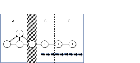
Figure 1: Schematic view of the wave functions involved in calculating decay widths by the GCM. See text for explanation.

The horizontal axis is a generator coordinate that includes fused or strongly interacting configurations (region A) as well as regions of separated clusters (regions B and C). In regions B and C the coordinate could be the operator measuring the separation of the clusters, Eq. (2) below. In region A or B the operator could be some other measure of shape such as the quadrupole moment operator. In the regions of separated clusters, we require that the asymptotic RGM wave functions are valid without any need for antisymmetrization between cluster. The line of horizontal arrows indicates that asymptotic relative coordinate wave function. The vertical line between region B and C is the chosen matching point between the two representations. Finally, the configuration $i$ in region A is the initial state whose decay width is the object of the theory.

In Sect. II below, we explore from a computational point of view the fidelity with which the relative-coordinate wave in the asymptotic region can be represented in a discrete basis of GCM configurations. Characteristics that can be compared are wave function overlaps, eigenstate energies, and logarithmic wave function derivatives. Sect. III deals with calculating $dn_{f}/dE$. It will be seen that a simple approach without the RGM wave functions is sufficient for rough estimates. However, when there are strong long-range potential fields in the final state, matching to the asymptotic RGM is unavoidable. We assess the accuracy of that procedure by determining its sensitivity to the choice of matching point $R$ and to the parameters defining the GCM configuration space.

II Continuous wave functions from a discrete basis

We are interested in the accuracy of relative-coordinate wave functions obtained from a discrete GCM basis. The problem of representing the center-of-mass wave function in a discrete basis of single-cluster GCM is nearly identical, and in this Section we simplify the notation accordingly. We start with a translationally invariant Hamiltonian $H$ that can be solved in the mean-field approximation to produce many-particle configurations $\Psi_{gcm}^{\alpha}$. These wave functions have the form of Slater determinants. External one-body fields $Q$ have been added to the Hamiltonian, with the strength of the fields adjusted to produce desired expectation values $\langle Q\rangle$, and the label $\alpha$ in $\Psi^{\alpha}_{gcm}$ includes this information. For the cm position of a single cluster containing $N$ particles, the field would obviously be $\vec{r}/N$. For the relative motion of two clusters along the $z$-axis, one can choose a dividing plane perpendicular to the axis located at some point $R$. The constraining operator is

$$z_{rel}=(z-R)\Theta(z-R)/N_{R}+(R-z)\Theta(R-z)/N_{L}$$ (2)

where $N_{R},N_{L}$ are the number of particles on each side.

We assume that the GCM wave function of a single cluster $\Psi^{\alpha}_{gcm}$ can be factorized into an internal wave function $\Psi^{\alpha}_{int}$ times a center-of-mass wave function $\psi_{cm}$,

$$\Psi^{\alpha}_{gcm}\left(\vec{r}_{1},\vec{r}_{2},\ldots\right) =\Psi^{\alpha}_{int}\left(\xi\right)\psi^{\alpha}_{cm}\left(\bar{z}_{\alpha},z_{cm}\right)$$ (3)

Here $\vec{r}_{1},\vec{r}_{2},\ldots$ are the coordinates of the constituent particles, $z_{cm}$ is a center-of-mass coordinate, and $\xi$ are unspecified internal coordinates. The parameter $\bar{z}_{\alpha}$ is the expectation value $\bar{z}_{\alpha}=\langle\alpha|z_{cm}|\alpha\rangle$ Factorization is a strong assumption, but there is some justification for it in nuclear theory. As was noted in some of the cited references, Eq. (3) is exact for the ground state of a many-particle system in a harmonic oscillator potential. Indeed, in the early studies the wave function were assumed to be harmonic oscillator eigenstates and thus factorizable. In a more general GCM treatment, information about the center-of-mass coordinate can be obtained by taking the overlap of the wave functions under displacement. It is an empirical fact that the overlap functions are close to Gaussian,

$$\int dz_{cm}\,\psi^{\alpha*}_{cm}\left(\bar{z}_{1},z_{cm})\right)\psi^{\alpha}_{cm}\left(\bar{z}_{2},z_{cm}\right)$$ (4)

$$\approx\exp(-(\bar{z}_{1}-\bar{z}_{2})^{2}/4s^{2})$$ (5)

for some size parameter $s$. Two examples from nuclear physics are shown in Fig. 2. The nuclei differ in particle number $N$ by an order of magnitude, but the length parameter $s$ in the fitted Gaussians differ only by a factor of $2.5$.

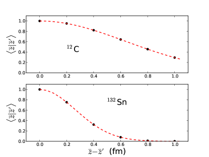
Figure 2: Overlaps of the nuclear ¹²C and ¹³²Sn mean-field wave functions as a function of cm coordinate displacement. Circles: overlaps of the GCM configurations; Dashed line: fit to a Gaussian function. Wave functions were calculated in a harmonic oscillator space containing 12 complete shells, using the Gogny D1S energy functional with no cm energy correction.

Combining the factorization assumption together with the observed near-Gaussian overlaps, the normalized cm wave function in Eq. (3) is given by

$$\psi_{cm}(\bar{z},z_{cm})=\left(\frac{1}{\pi s^{2}}\right)^{1/4}e^{-(\bar{z}-z_{cm})^{2}/2s^{2}}$$ (6)

The wave functions of physical interest are the stationary states in the space of the GCM configurations. These have the form

$$\begin{aligned} \Psi^{\lambda}_{gcm}&=\sum_{\alpha}a_{\alpha\lambda}\Psi_{gcm}^{\alpha}\end{aligned}.$$ (7)

where $a_{\alpha\lambda}$ is an amplitude and $\lambda$ is a label to distinguish the eigenstates. The amplitudes are obtained from the solutions of the non-Hermitian eigenvalue problem wi65

$$\sum_{\alpha}H^{gcm}_{\alpha^{\prime}\alpha}a_{\alpha\lambda}=E_{\lambda}\sum_{\alpha}N^{gcm}_{\alpha^{\prime},\alpha}a_{\alpha\lambda}.$$ (8)

Here $H^{gcm}$ and $N^{gcm}$ are the Hamiltonian and overlap matrices in the GCM basis. The amplitudes $a$ are normalized as

$$\sum_{\alpha,\alpha^{\prime}}a_{\alpha,\lambda}N^{gcm}_{\alpha,\alpha^{\prime}}a_{\alpha^{\prime},\lambda^{\prime}}=\delta_{\lambda,\lambda^{\prime}}$$ (9)

The machinery to calculate Eq. (8) is well developedbe03 and will not be discussed here. Suppose that the GCM basis states are all in the asymptotic region and the configurations are constructed on a uniform mesh $\bar{z}_{\alpha}=n\Delta z$. Then we can drop the subscript $\alpha$ on $\psi_{\alpha}$ and write

$$\psi^{\lambda}(z)=\sum_{n=n_{i}}^{n_{f}}a_{n,\lambda}\psi(n\Delta z,z)$$ (10)

where $n$ is an integer in the range $n_{i},n_{f}$. We now examine how well this wave function (and the associated eigenenergy $E_{\lambda}$) reproduces the exact $\psi(z)$ obtained by solving the Schrödinger equation for the RGM center-of-mass coordinate.

The most important parameter in the method is the mesh spacing; the accuracy that can be achieved with Eq. (10) depends on the dimensionless ratio $\Delta z/s$. There are two conflicting demands in the choice of mesh parameter. If $\Delta z>>s$, the spacing will be too sparse to approximate the continuum wave functions. On the other hand, if $\Delta z<<s$ the GCM space will be effectively overcomplete and the norm matrix $N^{gcm}$ will be nearly singular. The choice

$$\Delta z=5^{1/2}s$$ (11)

appears to be a reasonable compromise and we use is for most of the numerical examples. But one of the methods we examined to calculate decay width requires a somewhat finer mesh, as will be seen in Sec. III.

II.1 Plane waves

We start with a free-particle Hamiltonian on the infinite interval $z=(-\infty,\infty)$ and a GCM basis defined by Eq. (10-11). with the mesh space Eq. (11). By translational symmetry the GCM eigenstates can be expressed as

$$a_{n,k}=e^{ik\Delta z}$$ (12)

where $k$ is in the interval $(-\pi/\Delta z,\pi/\Delta z)$. The resulting wave function is

$$\psi_{k}(z)=\sum_{n}e^{ik\Delta z}\psi_{cm}(n\Delta z,z).$$ (13)

It should represent a plane wave of momentum $k$. As an example, Fig. 3 shows the components $\psi_{cm}(n\Delta z,z)$ in the range $(-\Delta z,\Delta z)$ and the wave function $\psi_{k}(z)$ for $k=0$ and $k=\pi/\Delta z$.

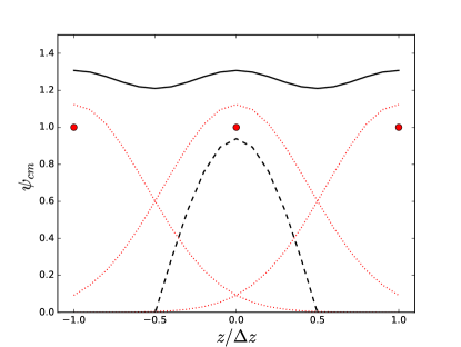
Figure 3: CM wave functions for a uniformly spaced basis in the CM coordinate, in units of $\Delta z$. The red circles are the amplitudes $a$ at the mesh points. Dotted lines are from individual GCM configurations; solid line is the approximate $k=0$ wave function; dashed line shows the positive part of the wave function for $k=\pi/\Delta z$.

Visually, the $k=0$ function (solid line) is quite flat, showing that it is close to a zero-momentum eigenstate. Of course there is a residual variation of the wave function due to the discrete basis. In the range of discretizations considered here, the relative variation can be estimated from the Poisson summation formula as

$$\frac{\psi}{\overline{\psi}}\sim 1\pm 2e^{-2\pi^{2}s^{2}/\Delta x^{2}}$$ (14)

where $\bar{\psi}$ is the average value of $\psi(z)$.

The figure also shows (dashed line) the positive part of the wave function for the maximum momentum contained in the basis, $k=\pi/\Delta x$. It is close to cosine function of argument $\pi z/\Delta z$, apart from normalization. Note that the corresponding sine function cannot be represented in the basis.

For a quantitative measure of the fidelity of the GCM representation, one can calculate the overlaps with true momentum eigenstates by Fourier transform. The probability $P_{k}(m)$ of momentum $k_{m}=k+m2\pi/\Delta z$ can be computed as

$$P_{k}(m)=\frac{\left|\int_{0}^{2dz\,\Delta z}e^{-ik_{m}z}\psi_{k}(z)\right|^{2}}{\int_{0}^{2\Delta z}dz\,\left|\psi_{k}(z)\right|^{2}}$$ (15)

Fig. 4 shows $P_{k}(0)$ over the range $k=(0,\pi/\Delta z)$. One sees that $P_{k}(0)$ is close to one up to $k\approx\pi/2\Delta z$. Beyond that the representation becomes poorer; at the upper limit it approaches $1/2$, with the $m=-1$ Fourier component taking nearly all of the remaining strength.

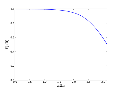
Figure 4: Probability of momentum $k$ in the GCM approximation $\psi_{k}$.

Another test of the representation is how well it reproduces the plane-wave energy spectrum,

$$E_{k}=\frac{\hbar^{2}k^{2}}{2M}.$$ (16)

Here $M$ is the mass of the cluster. The energy can be calculated the ratio of expectation values

$$E^{gcm}_{k}=\frac{\langle k|H^{gcm}|k\rangle}{\langle k|N^{gcm}|k\rangle}.$$ (17)

The results for the numerator and denominator are

$$\langle\psi_{k}|N^{gcm}|\psi_{k}\rangle=N\left(1+2\sum_{n=1}^{\infty}\cos(nk\Delta z)N^{gcm}_{0n}\right)$$ (18)

and

$$\langle\psi_{k}|H^{gcm}|\psi_{k}\rangle=N\left(H^{gcm}_{0n}+2\sum_{n=1}^{\infty}\cos(nk\Delta z)H^{gcm}_{0n}\right)$$ (19)

where $N$ is the number of basis states. The required overlap matrix elements are given by

$$N^{gcm}_{0n}=\exp(-n^{2}(\Delta z/2s)^{2}).$$ (20)

The matrix elements for the kinetic energy operator

$$T=-\frac{\hbar^{2}}{2M}\frac{\partial^{2}}{\partial z^{2}_{cm}}$$ (21)

are

$$T^{gcm}_{0n}=N^{gcm}_{0n}E_{0}\left(1-\frac{(n\Delta z)^{2}}{2s^{2}}\right).$$ (22)

where

$$E_{0}=\frac{\hbar^{2}}{4Ms^{2}}$$ (23)

is the expectation value of the kinetic energy in the wave function $\psi_{cm}$. $E_{0}$ is an important parameter setting the energy scale for the validity of the GCM basis as formulated here.

The accuracy of the GCM kinetic energy Eq. (17) under the conditions of the previous example may be seen in Fig. 5. The dashed line is the exact energy (Eq. (16)) and the solid line is the GCM result. There is a slight offset at $k=0$, but apart from that the error is less than 15% up to $k\approx\pi/2\Delta z$.

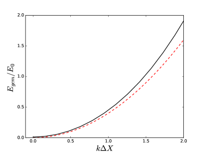
Figure 5: Solid line: free-particle energy versus momentum in the GCM approximation as discussed in the text; dashed line: exact energy from Eq. (16).

We judge the fit to be quite good for estimates not requiring wave function matching.

The wave-function matching can be carried out by renormalizing the $\psi(z)$ to reproduce both the amplitude and logarithm derivative of the asymptotic scattering wave function at $R$. Some preliminary indication of the error associated with this procedure be seen in Fig. 3: $\psi_{k}$ at $k=0$ undulates with an amplitude of about $4$ %. This suggests that normalization obtained by matching at different points $R$ would vary by a similar amount. Since the decay rate is quadratic in the normalization factor, this would cause an 8 % uncertainty in the calculated rate. This source of error will be treated in more detail in Sec. II.2.

II.2 Potential fields

We now add a potential $V$ to the Hamiltonian, with $V$ depending only on $z_{cm}$. The GCM matrix elements are computed as

$$V^{gcm}_{n,n^{\prime}}=\int dz\psi^{*}(n\Delta z,z)V(z)\psi(n^{\prime}\Delta z,z)$$ (24)

to give a Hamiltonian $H^{gcm}_{n,n^{\prime}}=T^{gcm}_{n,n^{\prime}}+V^{gcm}_{n,n^{\prime}}$. The energy scale $\hbar^{2}/2M\Delta z^{2}$ will set the permissible range of variation in $V$ when approximating the continuum wave functions. It is easy to show RS that the GCM representation is exact for a harmonic oscillator potential in the limit $\Delta z\rightarrow 0$.

We examine here the performance of the GCM taking $V$ to be a linear ramp potential in the negative $z$ region

$$V(z)=F|z|\Theta(-z).$$ (25)

where $F$ is a positive constant. The solutions to the Schrödinger equation for $H$ will be sinusoidal for $z>0$ and decay as a scaled reflected Airy function for large negative $z$. Fig. (6) compares the Schrödinger and the GCM wave functions for the set of parameters given in the caption. One sees that the GCM wave function roughly follows the sinusoidal form of the Schrödinger solution, but there are small unwanted undulations similar to those seen in Fig. 3. They are an artifact of the finite mesh spacing and can be reduced by decreasing it.

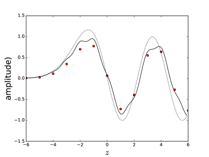
Figure 6: Comparison of the GCM and Schrödinger wave functions for the ramp Hamiltonian Eq.(25 with $F=0.4$. The GCM wave function is constructed in a basis of 13 configurations centered on the mesh $(-6\Delta z,6\Delta z)$. The circles show the amplitudes $a_{n,\lambda}$ for the third excited state at energy $E=1.029$. The corresponding $\psi_{\lambda}(z)$, shown as the solid line, is computed from Eq. (10) taking $s=\Delta z/5^{1/2}$. Amplitudes and wave function have been scaled by a factor of 2 to facilitate comparison with the Schrödinger function, shown as the dotted line. That wave function is sinusoidal for $z>0$ and has been normalized to $\sin(kz+\delta)$ for positive $z$.

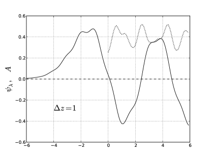
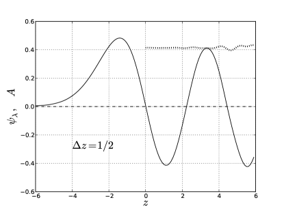
Figure 7: Solid line: wave function $\psi(z)$ for the ramp Hamiltonian. Dotted curve: sine function amplitudes $A$ from Eq. (26). Top and bottom panels show the results for mesh spacing of $\Delta z=1$ and 2, respectively. In the top panel, the variation in $A$ is $0.30-0.42$ for the range $R=1-3$. The variation reduced to $0.411<A<0.418$ in the bottom panel.

The critical test of the numerical approximations is how well the normalization of the GCM can be determined when matching to the Schrödinger solution. Assume that the GCM wave function has the form $\psi_{\lambda}(z)=A\sin(kz+\delta)$ at the chosen matching point $R$. Then $A$ is given by

$$A=\psi_{\lambda}(R)\frac{(k^{2}+{\cal L}^{2})^{1/2}}{k}$$ (26)

where $\cal L$ is the logarithmic derivative

$${\cal L}=\frac{1}{\psi_{\lambda}(R)}\left.\frac{d\psi_{\lambda}}{dz}\right|_{R}.$$ (27)

Fig. 7 shows the amplitude $A$ as a function of $R$ calculated this way. One sees that it fluctuates over a range of about 30% depending on the choice of $R$. The decay formula requires the square of the asymptotic amplitude, so the uncertainty in the calculated decay width will be as much as a factor of two. Clearly one would like to do better than this. One way is to decrease the mesh spacing, but there may be other ways based on properties of the unwanted undulations.

III Formulas for the cluster decay widths

Under the factorization Ansatz, the GCM wave function for a configuration of two separated clusters will have a product of the individual cm wave functions $\psi_{cm1}(z^{1}_{cm})\psi_{cm2}(z^{2}_{cm})$. Furthermore under the Gaussian assumption, that wave function can be written as a product of a Gaussian for the relative coordinate $z_{rel}=z^{1}_{cm}-z^{2}_{cm}$ times a Gaussian for another linear combination of $z^{1}_{cm}$ and $z^{2}_{cm}$. Thus the relative coordinate can be separated out and treated in exactly the same way as was done for $z_{cm}$ in the last section. Of course the mass $M$ in the kinetic energy of the final state is now the reduced mass of the two-cluster system.

We now return to Eq. (1). The state $i$ can be any configuration of the parent cluster that is stable under the mean-field Hamiltonian, with one qualification mentioned below. The $f$ channel is defined in the external region by the mean-field configurations of individual isolated daughter clusters. The channel needs to be defined in the internal region (A) as well. For this purpose, it would be helpful to introduce additional constraints to ensure that the added configurations are the ones with the largest Hamiltonian matrix elements connecting to the B-region configurations. For example, one could demand the basis be constructed using axially symmetric mean-field Hamiltonians. Then the orbitals are characterized by their angular momentum projections $J_{z}$ about the $z$-axis. The Hamiltonian matrix elements will be those which do not change the orbital occupancies with respect to $J_{z}$. A specific example is given in the Appendix; see also Ref. be18 . We note that an axial basis has been employed in chemical reaction theory to simplify the treatment of the interaction re74 . Also, the conservation of orbital symmetry is an important principle for understanding organic reactions wo65 .

Let us assume now that the GCM basis has been constructed for the $f$-channel chain and $H^{gcm}$ has been diagonalized to obtain eigenstates and their energies. The spectrum will be discrete since the basis is finite. This raises a technical issue in that the $f$ eigenstate should have the same energy as the initial state $i$. It would be straightforward to add a diagonal term to $H^{gcm}$ to tune the energy of one of the eigenstates to match $E_{i}$. If only matrix elements exterior to the matching point $R$ are adjusted, it shouldn’t matter how it is done. One last point is that the states $i$ and $f$ should be rigorously orthogonal; otherwise the perturbation formula Eq. (1) cannot be directly applied. Note that orthogonality is automatic the occupation numbers are different in a basis having an orbital symmetry.

In the numerical example below, we will also assume that the center and spread of the relative coordinate wave function of $i$ is the same as that of one of the $f$-channel configurations, say $n=n_{c}$. Then the matrix elements between $i$ and the $f$-channel configurations can be expressed as

$$H^{gcm}_{i,n}=v_{0}N^{gcm}_{n_{c},n}$$ (28)

where $v_{0}=H^{gcm}_{i,n_{c}}$. It should be emphasized that this assumption is only made for numerical convenience here; in practice the $(i,n)$ matrix elements would be calculated in the usual way using the GCM machinery. The expression for the squared interaction matrix element in Eq. (1) becomes

$$\langle i|H|f\rangle^{2}=v_{0}^{2}\left|\sum_{n}N^{gcm}_{n_{c},n}a_{n,\lambda}\right|^{2}.$$ (29)

Having taken care of the definitions of $i$ and $f$ and the interaction matrix element, the remaining task to determine the final state density $dn_{f}/dE$. There are several ways to proceed; we examine two of them. Method I is to extend the $f$ channel basis far into the asymptotic region. Then one can use the $f$-channel eigenfunctions and energies without an explicit introduction of an RGM wave function. For a rough estimate, we can take the energy difference between the eigenstates bracketing the initial state energy$E_{i}$, i.e.

$$\frac{dn_{f}}{dE}\approx\frac{1}{(E_{\lambda}-E_{\lambda-1})}\,\,\,\,{\rm Method~{}I}$$ (30)

where $E_{\lambda-1}<E_{i}<E_{\lambda}$.

Method II for determining $dn_{f}/dE$ is to match the $\psi(z)$ from the GCM to an asymptotic Schrödinger wave function in the final state. For the numerical example in Sect II, the asymptotic wave function is sinusoidal, and the match can be carried out with Eq. (26). The resulting density of states is

$$\frac{dn}{dE}\approx\frac{2M}{\hbar^{2}\pi k|A(R)|^{2}}.$$ (31)

A big advantage of Method II is that there can be arbitrary potential interactions in the final state. The generalization to arbitrary $V$ is textbook scattering theory. One first obtains the regular and irregular wave functions $u(z)$ and $w(z)$ of the scattering equation. Their relative amplitudes are set so that $w+iu$ is a pure outgoing wave. The GCM wave function $\psi$ is matched to a linear combination of the two as

$$\psi(R)\approx c_{1}u(R)+c_{2}w(R).$$ (32)

Then the density of states is given by

$$\frac{dn}{dE}\approx\frac{2M}{\hbar^{2}\pi(c_{1}^{2}+c_{2}^{2})W}\,\,\,\,{\rm Method~{}II}$$ (33)

where $W=uw^{\prime}-wu^{\prime}$ is the Wronskian of the two solutions.

We now carry out the numerical solution by the two methods applied to the ramp potential Eq (25). For this exercise, we take the interaction matrix element fom Eq. (29) placing the interaction point in the middle of the ramp, $z=z_{i}=-3\Delta z$. We assume that the energy of the initial state is $E_{i}=Fz_{i}$. For method I, we start with a basis of $N=13$ $f$-channel configurations as in the last section. More configurations will be added to the external end of the chain to assess the convergence of the method. We don’t attempt to tune the GCM Hamiltonian to produce an eigenstate at $E_{i}$ but simply interpolate between the two $f$-channel states bracketing $E_{i}$, i.e. taking weighted average over the two states $\lambda,\lambda^{\prime}$ to estimate $\langle i|H^{gcm}|f\rangle^{2}$. The results are shown in Fig. 8. One sees that the convergence is quite fast a function of $N$. For example, the calculated $\Gamma$ with $N=13$ configuration is within 10 % of the those calculated at $N=40-41$.

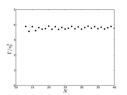
Figure 8: $n_{c}=4$ Decay width of a configuration $i$ to a channel $f$ in the potential field Eq. (25) as a function of the number of configurations in the $f$ channel. See text for the definition of the interaction Hamiltonian.

From the systematics, the calculated width can be estimated as

$$\Gamma_{I}=(3.8\pm 0.07)v^{2}_{0}.$$ (34)

For Method II, it is clear from Fig. 7 that a mesh spacing of $\Delta z=1$ would not permit a good estimate of the decay width. As shown in Fig. 7, reducing $\Delta z$ by a factor of 2 permits a much more accurate estimation of $A$. Using that mesh spacing the calculated decay width by Method II is

$$\Gamma_{II}=(3.77\pm 0.06)v^{2}_{0}.$$ (35)

We conclude that the two methods agree within their uncertainty and are accurate to a few percent for the chosen parameters.

IV Concluding remarks

It appears to us that GCM is a viable calculational framework in reaction theory involving composite particles as reaction partners. With the GCM, one can construct discrete configurations representing internal excitations of the clusters as well as the approximate channel states associated with decays into smaller clusters.

The most critical approximation is the factorizability in the GCM of internal and cm wave functions, Eq. (3). This has a direct impact on the kinetic Hamiltonian. It was found in an early study of the GCM method pe62 it was found that the calculated overall inertial mass of a composite particle may be incorrect. The problem doesn’t arise in the present treatment because the factorizability Ansatz permits the kinetic operator to be evaluated in both the single-particle coordinate representation and in the representation with the explicit cm coordinate. It might not be a good approximation in practice if there are important contributions to the GCM configuration from excited internal states having different energies and cm wave functions. However, if the energies are very different, an even more fundamental assumption is violated. Namely, it would call into question the utility of the mean-field approximation to provide a good description of the structure and energy of the lowest internal state. We note that there is also an extensive literature for dealing with the cm wave function in mean-field theory; see for example Ref. gl74 . Obviously, more study is needed to determine how reliable the Ansatz is.

As presented here, a severe limitation of the GCM method is that the $f$-channel configurations should have energies that don’t vary much from each other on an scale set by the zero-point cm kinetic energies. In principle, this can be ameliorated by including in some way the kinetic energy into the GCM constraints. This is can be implemented by constraining the expectation of the momentum operator $p_{rel}=\partial/i\partial z_{rel}$ (as well as $z_{rel}$) in constructing the configurations. This requires modifying the GCM machinery to deal with complex arithmetic, but that should be a straightforward task. It has also been suggested to project on states of good momentumpe62 ; wo72 , but the procedure is challenging from a computational point of view.

There are two distinct regions where the theory of decay widths might be applied. At low energies, one might expect that the internal states are more widely spaced than their decay widths. In this weak-coupling limit, Eq. (1) can be applied to the individual resonances. At higher energies and under certain conditions on the Hamiltonian, the decay widths may exceed the level spacings. Here the individual decay widths are not of interest but only their statistically weighted averages. The relevant physical quantity now becomes the transmission coefficient $T$ between fused and separated clusters. In the weak coupling limit it can be expressed as

$$T=2\pi\left\langle\frac{\Gamma}{D}\right\rangle$$ (36)

where the brackets denote averaging and $D$ is the level spacing. For large $\Gamma/D$ the transmission coefficient approaches its unitary limit of $T=1$ and there is no need for high accuracy even in the calculation of the average.

V Acknowledgments

We would like to acknowledgment discussions with T. Kawano and L. Robledo on the physics of nuclear fission, motivating some of the questions addressed in this work.

VI Appendix: example of an $f$ channel chain

Extension of the $f$-channel chain into region $A$ requires finding the configurations that have the largest off-diagonal Hamiltonian matrix elements to the chain. This problem was studied in Ref. de75 for the nuclear reaction ¹⁶O + ¹⁶O $\rightarrow$ ³²S. The authors assumed axial symmetry in constructing of the basis. They found that only one particular configuration in the fused system had a large Hamiltonian matrix element. The character of that configuration can be understood in terms of the orbital fillings with respect to $J_{z}$, as was carried out in Ref. be16 . We summarize the argument here. Each oxygen configuration is constructed from the elementary shell model, filling the lowest $s$- and $p$-shell orbitals. The orbitals are assumed to be independent of nucleon spin and isospin. Thus, each spatial orbital is occupied by 4 nucleons. The $s$ and the three $p$ orbitals are classified by the angular momentum $L_{z}$ about the $z$ axis; the occupation numbers are $(8,4,4)$ for $L_{z}=(0,+1,-1)$. These occupancies are doubled for two oxygen nuclei aligned along the $z$ axis. Thus we seek configurations in the sulfur nucleus having occupancies $(16,8,8,0,...)$ for $L_{z}=(0,+1,-1,+2,-2,...)$. We have added $L_{z}=\pm 2$ to the list because the lowest configurations in that nucleus begin to fill the $d$ shell. In addition to the angular momentum quantum number, the orbitals can be considered to have a good parity. In the initial configuration there is the same number of particles in each parity orbital. Thus, 8 of the 16 $L_{z}=0$ orbitals are even parity and 8 are odd, and so on. The combined quantum numbers are preserved in the $f$ chain, and the possible configurations in the combined system are quite limited. Following the simple shell model, the configuration satisfying these fillings has completely filled $s$ and $p$ shells, 12 particles in the $sd$ shell, and 4 particles in the next higher shell. The Hamiltonian matrix elements of the external $f$ chain to this configuration is found to be orders of magnitude larger than to other configurations of the combined system de75 . So for this case at least a clear separation between the $f$ chain members and the other configurations is possible.

References

- (1) P. Navratil, S. Quaglioni, G. Hupin, et al., Phys. Scr. 91 053002 (2016).
- (2) Z. Sun, H. Guo, and D.H. Zhang, J. Chem. Phys. 132 084112 (2010).
- (3) D.L. Hill and J.A. Wheeler, Phys. Rev. 89 1102 (1953).
- (4) M. Bender, P.H. Heenen, and P.G. Reinhard, Rev. Mod. Phys. 75 121 (2003).
- (5) M. Trsic and A. de Silva, Electronic Atomic and Molecular Calculations, (Elsevier, Amsterdam, 2007).
- (6) K. Kubodera and K. Ikeda, Prog. Theor. Phys. 42, 740 (1969).
- (7) H. Horiuchi, Prog. Theor. Phys. 43, 375 (1970).
- (8) M. Harvey and A. S. Jensen, Nucl. Phys. A179, 33 (1972).
- (9) F. Tabakin, Nucl. Phys. A182, 497 (1972).
- (10) N.B. de Takacsy, Phys. Rev. C5 1883 (1972).
- (11) H. Horiuchi and Y. Suzuki, Prog. Theor. Phys. bf 49, 1974 (1973).
- (12) R. Beck, J. Borysowicz, D. M. Brink, and M. V. Mihailović, Nucl. Phys. A244, 45 (1975).
- (13) H. Friedrich and K. Langanke, Nucl. Phys. A 252 47 (1975).
- (14) H. Hüsken, Nucl. Phys. A291, 206 (1977).
- (15) M. Onsi and J. Le Tourneux, Can. J. Phys. 58 612 (1980).
- (16) A. Bulgac, P. Magierski, et al., Phys. Rev. Lett. 116 122504 (2016).
- (17) J.F. Berger, M. Girod, and D. Gogny, Comp. Phys. Comm. 63 365 (1991).
- (18) J.H. Wilkinson, ”The Algebraic Eigenvalue Problem”, (Oxford University Press, Oxford, 1965) Sect. 5.68.
- (19) P. Ring and P. Schuck, “The Nuclear Many-Body Problem”, (Springer, Heidelberg, 1980) Sec. 10.6.3
- (20) G.F. Bertsch, W. Younes and L.M. Robledo, Phys. Rev. C 97 064619 (2018).
- (21) T.N.Rescigno, C. McCurdey and V. McKoy, Phys. Rev A 10 2240 (1974).
- (22) R.B. Woodward and R. Hoffman, J. Am. Chem Soc. 87 395 (1965).
- (23) R. Peierls and D. Thouless, Nucl. Phys. 38 154 (1962).
- (24) Gloeckner and R. Lawson, Phys. Lett. B 53 313 (1974).
- (25) C.W. Wong, Nucl. Phys. A 197 193 (1972).
- (26) H. H. Deubler and T. Fliessbach, Nucl. Phys. A238, 409 (1975).
-
(27)
G.F. Bertsch and J.M. Mehlhaff, EPJ Web of Conferences
122 01001 (2016).