Dimension Reduction for Origin-Destination Flow Estimation:
Blind Estimation Made Possible

Abstract.

This paper studies the problem of estimating origin-destination (OD) flows from link flows. As the number of link flows is typically much less than that of OD flows, the inverse problem is severely ill-posed and hence prior information is required to recover the ground truth. The basic approach in the literature relies on a forward model where the so called traffic assignment matrix maps OD flows to link flows. Due to the ill-posedness of the problem, prior information on the assignment matrix and OD flows are typically needed.

The main contributions of this paper include a dimension reduction of the inquired flows from $O\left(n^{2}\right)$ to $O\left(n\right)$, and a demonstration that for the first time the ground truth OD flows can be uniquely identified with no or little prior information. To cope with the ill-posedness due to the large number of unknowns, a new forward model is developed which does not involve OD flows directly but is built upon the flows characterized only by their origins, henceforth referred as O-flows. The new model preserves all the OD information and more importantly reduces the dimension of the inverse problem substantially. A Gauss-Seidel method is deployed to solve the inverse problem, and a necessary condition for the uniqueness of the solution is proved. Simulations demonstrate that blind estimation where no prior information is available is possible for some network settings. Some challenging network settings are identified and discussed, where a remedy based on temporal patterns of the O-flows is developed and numerically shown effective.

1. Introduction

The origin-destination (OD) flow estimation problem can be stated as follows. Consider a network $\mathcal{G}\left(\mathcal{N},\mathcal{L}\right)$ specified by the set of nodes $\mathcal{N}$ (also known as vertices) and links $\mathcal{L}$ (also called edges). Suppose that the quantities of link flows are given during the time horizon involving multiple consecutive sampling time intervals. The task is to estimate the volume of the OD flows.

OD flow estimation is essential to many network analysis tasks. This paper focuses on transportation networks though the developed approach can be extended to other types of networks. In the transportation community, it has been widely accepted that OD information reflects the travel demands and plays an essential role in long term infrastructure planning, traffic prediction under unexpected changes in the infrastructure or the traffic status, and commercial applications linked to population migration [1], and serves as an important input to traffic simulation models [2, 3]. Despite its importance, accurate OD information is difficult, expensive, and sometimes impossible to be obtained. The old fashioned household survey data are expensive and time-consuming to collect and typically incomplete and biased [4, 5]. Commercial transportation service data from taxi and Uber are highly biased towards commercial activities. Recently modern technologies, for instance GPS, mobile phone, automatic plate recognition systems, automatic vehicle identification systems, and combinations of these systems, provide new data sources and new opportunities for acquiring OD information [6, 7, 8, 9, 10, 11]. However, the data are highly privacy-sensitive and sometimes error-prone.

The problem of interest is to infer OD flows from the link flows. It is ill-posed as the number of link flows (observations) is typically much less than that of OD flows (unknowns). Let $n_{n}$ be the number of the nodes in the network and $n_{\ell}$ be the number of the links. Let $n_{\ell}=cn_{n}$ where $c\in\mathbb{R}^{+}$ denotes the average number of links per node. In a transportation network, it is typical that $2\leq c\leq 4$. At the same time, the number of OD flows can be as large as $n_{n}^{2}$. Even when restricting the distance between the origin and destination nodes, the number of possible OD flows can be still much larger than that of link flows. The inverse problem typically does not admit a unique solution.

In the literature, a common approach is based on a linear forward model that maps OD flows to link flows. Refer to the linear operator that maps OD flows to link flows as traffic assignment [4, 5, 1] (also known as link choice proportions [12, 13], or path proportions [14, 15]). It gives the fraction of an OD flow passing through a specific link. The assignment matrix based approach requires prior information on both the assignment matrix and the OD flows: it is typically assumed that either the assignment matrix or its approximation is given based on historical data or traffic modeling; prior information on the inquired OD flows includes historical data, statistical models, temporal and/or spatial relationship among the flows, etc. Beyond the linear model, nonlinear models such as user equilibrium model [16, 17, 14, 18] and network loading model [19, 20, 18] have been deployed to describe the complex relationships between OD flows and link flows. Prior knowledge in terms of domain knowledge or historical data is also needed in addressing the ill-posedness of the OD flow estimation problem.

In this paper, the fundamental question of interest is whether the ill-posedness of the inverse problem can be addressed with no or little prior information, i.e., whether blind estimation is possible. This paper adopts the assignment matrix based linear model for simplicity and the purpose of proof-of-concept. We assume that the traffic assignment matrix is unknown but fixed during the whole time horizon. The OD flows are dynamic, meaning that the OD flows vary across different sampling time intervals.

The main contributions of this paper are summarized in the following.

• A new linear model is developed to allow substantial dimension reduction of the inquired flows from $O\left(n^{2}\right)$ to $O\left(n\right)$. More specifically, define a flow originating from a node as an O-flow. A linear model is constructed to map O-flows to link flows. With a slight abuse of terminology, refer to the corresponding linear operator also as traffic assignment matrix. (The two different assignment matrices, one corresponding to OD flows and the other O-flows, can be distinguished according to the context.) The O-flows together with the corresponding assignment matrix preserve the OD flow information. At the same time, the number of O-flows is at most the number of the nodes in the network, which is typically less than the number of links and much less than the number of OD flows.

• It is numerically demonstrated that for the first time the ground truth OD flows can be uniquely identified without any prior information of either the flows or the traffic assignment. In this paper, the OD flow information is inferred by jointly estimating both the O-flows and the corresponding assignment matrix. An iterative algorithm is developed to solve the joint estimation problem based on the Gauss-Seidel method. Simulations in Section 5 show that the ground truth OD flows can be estimated with high accuracy for bidirectional networks. In one tested scenario, 1660 OD flows are accurately estimated from 224 link flows without any prior information. According to the authors’ knowledge, no similar result has been reported before in the literature.

• A necessary condition is derived for the uniqueness of the solution of the O-flow model. Based on this necessary condition, we show that in general unidirectional networks do not admit unique solutions. A remedy is proposed to promote a unique solution by assuming temporal patterns in O-flows, in particular that the coefficients of the discrete cosine transform (DCT) of O-flows have only a few significant components. Numerical simulations have demonstrated the effectiveness of this remedy. Here, the only prior information used is that O-flows are sparse in the DCT transform domain. There is no need for historical data, or the knowledge which DCT coefficients are nonzero.

In summary, blind estimation is made possible thanks to the substantial dimension reduction of the new linear model.

As a starting point, this paper focuses on a simple linear model involving a static assignment matrix. In reality, the relationship between OD flows and link flows is nonlinear according to the fundamental diagram of traffic flow. Even in the local linear approximation regime, the assignment matrix can be dynamic in real life situations. Our new model and approach can be adapted and extended to address more complicated scenarios, which we leave as future work.

This paper is organized as follows. Section 2 reviews popular models and techniques in the literature briefly. Section 3 introduces our linear model used for OD flow estimation. Section 4 describes the computational procedure, derives a necessary condition for the uniqueness of the solution, and analyzes unidirectional networks. Simulation results are presented in Section 5 to demonstrate the feasibility for blind estimation. Conclusions and possible future work are given in Section 6.

2. Models for OD Estimation in literature

Directed graphs $\mathcal{G}\left(\mathcal{N},\mathcal{L}\right)$ are considered in this paper. Denote the traffic flow cont of the link from a node $i$ to its adjacent node $j$ by $y_{ij}$. Similarly the traffic flow count from an origin node $o$ to a destination node $d$ is denoted by $s_{od}$. Assume that the network has $n_{n}$ many nodes, $n_{\ell}$ many links, and $n_{{\rm OD}}$ many OD pairs.

2.1. Forward Models

Group the link flows $y_{ij}$ into a vector $\bm{y}$. It is clear that $\bm{y}\in\bar{\mathbb{R}}^{n_{\ell}}$ where $\bar{\mathbb{R}}:=\mathbb{R}^{+}\bigcup\left\{0\right\}$ is the set of non-negative real numbers. Let $\bm{s}\in\bar{\mathbb{R}}^{n_{{\rm OD}}}$ denote the OD flow vector. The most popular linear model in the literature [21, 5, 22, 23, 24, 25] is given by

(2.1) $$\bm{y}=\bm{A}\bm{s},$$

where the matrix $\bm{A}$ is referred to as traffic assignment matrix, and its entries $a_{ij,od}$ gives the fraction of OD flow $s_{od}$ passing the link from $i$ to $j$.

Finer time resolution can be added to the above model. Refer to the time window under which the link flow data are collected as sampling time interval, and the time period of all the consecutive sampling time intervals as time horizon. Model (2.1) implicitly assumes that all the OD flows finish in one sampling time interval, which is reasonable in real life when the sampling time interval is sufficiently long, for example, a day long. With finer time resolution, for example the sampling time interval is of ten minutes long, multiple sampling time intervals may be involved during the lifetime of OD flows. The linear relations from OD flows to link flows are then described by a convolution form:

(2.2) $$\bm{y}^{t}=\sum_{\tau=1}^{\tau_{\max}}\bm{A}^{\tau}\bm{s}^{t-\tau+1},\;\mbox{or equivalently }\bm{y}^{t}=\bm{A}^{t}*\bm{s}^{t},$$

where $\bm{y}^{t},$ $\bm{A}^{t}$, and $\bm{s}^{t}$ are the link flow, traffic assignment matrix, and the OD flow at time interval $t$ respectively, $\tau_{\max}\in\mathbb{Z}^{+}$ is the maximum number of consecutive sampling time intervals involved for OD trips, and the symbol $*$ denotes a convolution which is commonly used in signal processing community. Refer to this model as multi-step model. On one hand, it provides finer time resolution. On the other hand, it involves more unknown variables and more prior information is needed to solve the inverse problem.

It is noteworthy that both linear models (2.1) and (2.2) assume that the traffic assignment matrix $\bm{A}$ is independent of the OD flows $\bm{s}$. This model is often referred to as a separable model in the literature. In real life scenarios, the assignment matrix $\bm{A}$ and the OD flows are correlated (non-separable) according to the fundamental diagram of traffic flow. A non-separable model results in a nonlinear model, e.g., user equilibrium model [21, 16, 17, 14, 18], and goes beyond the scope of this paper.

2.2. OD Estimation: Solving the Inverse Problem

The inverse problem of OD estimation is severely ill-posed because the number of OD flows (unknown variables) can be much larger than that of observed link flows. To address this issue, prior information on both the assignment matrix and the OD flows is necessary. Based on different assumptions about the prior information, different techniques have been developed to solve the inverse problem. In this following, we shall discuss some representative approaches. As OD flow estimation has been an active research topic for many decades, we can only include a small subset of the literature below.

In the works [4, 21], gravity models and entropy maximizing principle have been used to choose one solution (of the inverse problem) from all feasible ones. The basic form of gravity models is to approximate the OD flow $s_{od}$ by

$$s_{od}=bR_{o}R_{d}c_{od}^{-r},$$

where $b$ and $r$ are parameters for calibration, $R_{o}$ and $R_{d}$ represent information (e.g. population, employment, the mean income of the residence) of the origin and the destination respectively, and $c_{od}$ is the cost of traveling from $o$ to $d$. In entropy maximizing models [4, 21, 26, 25], among all feasible solutions satisfying $\bm{y}=\bm{A}\bm{s}$, the one that maximizes the entropy function $-\sum_{o,d}\left(s_{od}\ln s_{od}-s_{od}\right)$ is of interest. A variation of this is given by the information minimizing model [21, 26], of which the solution has a very similar form to that of the entropy maximizing model.

When historical data of the OD flows are available, a popular approach is the Generalized Least Squares (GLS) estimator. Assume that both the link flow measurement errors and OD flow approximation errors can be modeled by using multivariate normal distribution. The GLS estimator is given by [5, 13, 12]

(2.3) $$\begin{array}[]{c}\min_{\bm{s}}\;\left(\bm{A}\bm{s}-\bm{y}\right)^{T}\bm{W}^{-1}\left(\bm{A}\bm{s}-\bm{y}\right)\end{array}+\left(\bm{s}-\bm{s}^{H}\right)^{T}\bm{V}^{-1}\left(\bm{s}-\bm{s}^{H}\right),$$

where $\bm{W}$ and $\bm{V}$ are the covariance matrices and assumed to be known a priori. The multivariate normal distribution may result in negative values of OD flows. One way to address this is to add a constraint that the inquired OD flows must be non-negative [22]. Another way is to replace the Gaussian distribution with the Poisson distribution [27, 13, 12, 28] which is non-negative, describes the traffic behavior better, but is computationally more costly. As a fundamental framework, GLS has been adopted and adapted in many other works, e.g., [29, 11, 30].

To design and manage modern intelligent transportation systems, it is important to model the dynamic nature of the OD flows where the sampling time interval is much less than a day. The dynamics of the OD flows further increase the number of unknowns and calls for extra prior information to cope with the ill-posedness. In [31, 24], the dynamics of the OD flows is modeled by an auto-regressive process. Let $\partial\bm{s}^{t}=\bm{s}^{t}-\bm{s}^{t,H}$ be the deviations of OD flows $\bm{s}^{t}$ from the historical data $\bm{s}^{t,H}$. The auto-regressive model assumes

$$\partial\bm{s}^{t}=\sum_{\tau=1}^{q}\bm{B}^{\tau}\partial\bm{s}^{t-\tau}+\bm{w}^{t},$$

where $\bm{B}^{\tau}\in\mathbb{R}^{n_{OD}\times n_{OD}}$ represents the linear contribution of $\partial\bm{s}^{t-\tau}$ to $\partial\bm{s}^{t}$ and are assumed to be known a priori, and $\bm{w}_{t}$ denotes the errors. The multi-step linear model (2.2) can be equivalently written as

$$\partial\bm{y}^{t}=\sum_{\tau=1}^{\tau_{\max}}\bm{A}^{\tau}\partial\bm{s}^{t-\tau+1}+\bm{v}^{t},$$

where $\partial\bm{y}^{t}=\bm{y}^{t}-\sum_{\tau=1}^{\tau_{\max}}\bm{A}^{\tau}\bm{s}^{t-\tau+1,H}$ and $\bm{v}_{t}$ describes the errors. Assume that $\bm{w}^{t}$ and $\bm{v}^{t}$ are multivariate normal distributed with mean zero and covariance matrices $\bm{W}$ and $\bm{V}$ respectively. A GLS estimator similar to (2.3) can be then applied. Based on the auto-regressive modeling, a principal component analysis has been applied to $\bm{s}^{t}$ for the purpose of further dimension reduction [32]. Another way to explore the temporal correlations of OD flows is to pool identical time periods over days from the same day category [3].

Spatial structures of the OD flows can be also used to mitigate the ill-posedness. In stead of considering traffic flows between any pair of nodes, one can simplify the network and the analysis by aggregating nodes into zones represented by virtual nodes, connecting them by virtual links, and analyzing the traffic flows between pairs of the virtual nodes. This conventional traffic modeling has been adopted by many works, e.g. [13, 12, 33], to cope with limited data and/or computational power. It is typically left as decisions for domain experts to decide the zone construction, including the number of zones, the position of the virtual nodes, and the virtual links connecting virtual nodes. In recent work [29], two techniques are used to reduce the spatial complexity of the network: automatic zoning and sparsity regularization. Instead of grouping multiple nodes, the aim of automatic zoning is to select individual nodes as centers of traffic analysis zones in order to find a Pareto optimal point for the bi-criteria objective

$$\underset{\bm{b}\in\left\{0,1\right\}^{n_{n}}}{\min}\;\left\{\left\|\bm{b}\right\|_{0},\left\|\bm{y}-\bm{A}^{\left(\bm{b}\right)}\bm{s}^{\left(\bm{b}\right)}\right\|_{2}^{2}\right\},$$

where the entries of $\bm{b}$ indicate which nodes are chosen and which are not, the pseudo-norm $\left\|\cdot\right\|_{0}$ counts the number of nonzero elements, and $\bm{A}^{\left(\bm{b}\right)}$ and $\bm{s}^{\left(\bm{b}\right)}$ represent truncation of $\bm{A}$ and $\bm{s}$, respectively, based on the nonzero elements of $\bm{b}$. Under some assumptions, this bi-criteria objective leads to a constrained nonconvex optimization formulation for automatic zoning. A heuristic algorithm is also developed. After automatic zoning, the authors further assume that “for all but the coarsest of zonings”, OD flows should be sparse in the sense that most OD flows are so small to be safely approximated by zero. An $\ell_{1}$-regularization term is added to the GLS estimator to promote the sparsity of the estimated OD flows, resulting in

$$\underset{\bm{s}\geq\bm{0}}{\min}\;\left(\bm{y}-\bm{A}\bm{s}\right)^{T}\bm{W}^{-1}\left(\bm{y}-\bm{A}\bm{s}\right)+\lambda\left\|\bm{s}\right\|_{1},$$

where $\bm{A}$ and $\bm{s}$ are the assignment matrix and OD flows after zoning, and $\lambda\in\mathbb{R}^{+}$ is a properly chosen constant to balance data fidelity and solution sparsity.

It can be observed that all the approaches discussed above heavily rely on the assumption that either the assignment matrix or its approximation is known a priori. In reality, such information has to come from somewhere. The simplest approach is the so called “all-or-nothing” assignment [29, p. 153, and references therein] where only one path is for one OD trip and the path is chosen to be the one with the least travel cost (distance or average travel time). Similarly, one can also allow multiple paths for OD trips and assign a probability for these paths based on either historical data or a cost measure. The difficulties [21] include, but are not limited to, the availability/sufficiency of historical data, the cost measure to choose, possibly different perceptions and objectives from different drivers in different situations, imperfect knowledge of the alternative routes, and the dynamics of the assignment matrix under different road/traffic conditions. The last difficulty can be addressed by local linear approximation of the assignment matrix [34, 35] or a user equilibrium based assignment. However, these techniques result in a nonlinear model that relies on knowledge of the OD flows, and hence goes beyond the scope of this paper.

3. A New Forward Model for OD Flow Estimation

In the light of the above, the main technical difficulty of using the standard linear models (2.1,2.2) for OD flow estimation comes from the large dimension of the unknowns. The focus of this section is to present a new forward model which reduces the dimension of the inquired flows from $O\left(n_{n}^{2}\right)$ to $O\left(n_{n}\right)$.

3.1. O-flow Based Models

We build a linear forward model not directly involving the inquired OD flows. It is built on the traffic flows that are specified with their origins but not their destinations, henceforth referred to as O-flow. Let $x_{o}$ denote the flow originating from the node $o$, i.e., $x_{o}=\sum_{d\neq o}s_{od}$. Define the O-flow vector as $\bm{x}=\left[x_{1},\cdots,x_{o},\cdots,x_{n_{O}}\right]^{T}$, where $n_{O}$ is the number of valid origins in the network. Let $p_{ij,o}$ denote the proportion of the O-flow $x_{o}$ that passes the link from $i$ to $j$. Denote the traffic assignment matrix associated with O-flows $\bm{x}$ by $\bm{P}$ of which the entries are $p_{ij,o}$. Assume static traffic assignment and dynamic flows. When the sampling time interval is longer than the trip time, one has the following single step model

(3.1) $$\bm{y}^{t}=\bm{P}\bm{x}^{t},\quad t=1,2,\cdots,n_{T},$$

where $n_{T}\in\mathbb{Z}^{+}$ denotes the number of sampling time intervals involved in the time horizon. Otherwise, one has a multi-step model where

(3.2) $$\bm{y}^{t}=\sum_{\tau=1}^{\tau_{\max}}\bm{P}^{\tau}\bm{x}^{t-\tau+1},\;\mbox{{\rm or }}\bm{y}^{t}=\bm{P}^{t}*\bm{x}^{t},\quad t=1,2,\cdots,n_{T},$$

where $\tau_{\max}$ is the maximum trip time.

Remark 1.

In the sequel, we will sometimes use single step models for illustrate simplicity. The simulations are based on the multi-step model (3.2).

It is clear that the number of O-flows $n_{O}$ is upper bounded by $n_{n}$. In typical transportation networks, the average number of links per node, denoted by $c\in\mathbb{R}^{+}$, is larger than 1. In this case, the number of equations $n_{\ell}=cn_{n}$ is more than the number of unknown O-flows. The inverse problem is then well-posed when the assignment matrix is given and of full column rank (which is possible only when $n_{\ell}\geq n_{O}$).

The new model does not involve OD flows directly but preserves the OD flow information.

Theorem 2.

All the OD flows can be inferred from the given O-flows and the corresponding assignment matrices.

Proof.

In the single step model (3.1), the OD flow $s_{od}$, $o\neq d$, can be calculated from

(3.3) $$s_{od}=x_{o}\left(\sum_{i}p_{id,o}-\sum_{j}p_{dj,o}\right),$$

where the term $x_{o}\sum_{i}p_{id,o}$ calculates the inflow to the node $d$ that originates from the node $o$, the term $x_{o}\sum_{j}p_{dj,o}$ gives the outflow from the node $d$ that originates from the node $o$, and the difference between them is clearly the flow ending at the node $d$ and originating from the node $o$.

Similar arguments can be applied to the multi-step model (3.1), resulting in

(3.4) $$s_{od}^{t}=x_{o}^{t}\left(\sum_{\tau=1}^{\tau_{\max}}\sum_{i}p_{id,o}^{\tau}-\sum_{\tau=1}^{\tau_{\max}}\sum_{j}p_{dj,o}^{\tau}\right).$$

∎

Remark 3.

The concept of O-flows has been mentioned in the literature, e.g., [3]. However, when coming to OD flow estimation, none of existing works builds the inverse problem on O-flows.

Remark 4.

A model similar to (3.1) can be constructed based on the D-flow as well (D stands for destination) which also allows for dimensional reduction and the preservation of OD flow information. More specifically, let $x_{d}$ be the flows ending at the node $d$, and $p_{ij,d}$ be the proportion of $x_{d}$ passing the link from $i$ to $j$. Then OD flows can be computed via

$$s_{od}=x_{d}\left(\sum_{j}p_{oj,d}-\sum_{i}p_{io,d}\right)$$

for single step model, and

(3.5) $$s_{od}^{t}=\sum_{\tau=1}^{\tau_{\max}}x_{d}^{t+\tau}\left(\sum_{j}p_{oj,d}^{\tau}-\sum_{i}p_{io,d}^{\tau}\right)$$

for multi-step model. The slight difference between (3.5) and (3.4) comes from the definition of $s_{od}^{t}$ which describes the OD flow $s_{od}$ starting at the time interval $t$. The models based on O-flow and D-flow are interchangeable. This paper focuses on the O-flow model only.

3.2. Connections and Differences of Models

On one hand, our model preserves the OD flow information via (3.3,3.4). On the other hand, the number of unknown variables (including those in the assignment matrices and the flows) in our new model are substantially reduced from the standard model (2.1,2.2). An educated instinct is that some information must get lost by this dimension reduction. To characterize the exact information got lost and to understand its importance, we need to study the relationship among three different models built upon path flows, OD flows, and O-flows, respectively. For simplicity of discussion, we focus on a single snapshot of single step models.

Many papers [36, 24, 3] in the literature use path flow models. For a given path $\bm{p}$ specified by $o\rightarrow i\rightarrow\cdots\rightarrow d$, denote the flow along this particular path by $s_{\bm{p}}^{{\rm path}}$. Group all path flows into a vector to form path flow vector $\bm{s}^{{\rm path}}$. Then the observed link flows are given by

$$\bm{y}=\bm{A}^{{\rm path}}\bm{s}^{{\rm path}},$$

where $\bm{A}^{{\rm path}}$ is the path incidence matrix where

$$A_{ij,\bm{p}}^{{\rm path}}=\begin{cases}1&\text{ if the path }\bm{p}\text{ involves the link }ij,\\ 0&\text{ otherwise.}\end{cases}$$

Figure 3.1. An example of 3-by-3 unidirectional network.

The path flow model contains more information than the OD flow model does. Let $\mathcal{P}_{od}$ be the set of all paths with origin $o$ and destination $d$. It is straightforward to verify that

$$s_{od}=\sum_{\bm{p}\in\mathcal{P}_{od}}s_{\bm{p}}^{{\rm path}},\;{\rm and}$$

(3.6) $$a_{ij,od}=\frac{\sum_{\bm{p}\in\mathcal{P}_{od}}a_{ij,\bm{p}}^{{\rm path}}s_{\bm{p}}^{{\rm path}}}{\sum_{\bm{p}\in\mathcal{P}_{od}}s_{\bm{p}}^{{\rm path}}}.$$

However, the OD flow model does not fully characterize the path flow model in general. Specifically, we use the following example to illustrate that the lost information is the path selection information when multiple paths associated with the same OD share the same subset of links.

Example 5.

In the unidirectional network in Figure 3.1, consider the four different paths $\bm{p}_{1}=1\rightarrow 2\rightarrow 5\rightarrow 6\rightarrow 9$, $\bm{p}_{2}=1\rightarrow 2\rightarrow 5\rightarrow 8\rightarrow 9$, $\bm{p}_{3}=1\rightarrow 4\rightarrow 5\rightarrow 6\rightarrow 9$, and $\bm{p}_{4}=1\rightarrow 4\rightarrow 5\rightarrow 8\rightarrow 9$ which correspond the same OD trip from 1 to 9. Suppose that the observed link flows on all involved links are $c_{l}$ with $c_{l}>0$. The corresponding OD flow model is unique: $s_{19}=2c_{l}$ and $a_{ij,19}=\frac{1}{2}$ for all involved links. However, the consistent path flow model is not unique: that $s_{\bm{p}_{1}}^{{\rm path}}=s_{\bm{p}_{4}}^{{\rm path}}=c_{l}$ and $s_{\bm{p}_{2}}^{{\rm path}}=s_{\bm{p}_{3}}^{{\rm path}}=0$, that $s_{\bm{p}_{1}}^{{\rm path}}=s_{\bm{p}_{4}}^{{\rm path}}=0$ and $s_{\bm{p}_{2}}^{{\rm path}}=s_{\bm{p}_{3}}^{{\rm path}}=c_{l}$, and any convex combination of these two cases can give the exactly same link flows.

Similarly the OD flow model contains more information than the O-flow model does. The O-flow model can be derived from the OD flow model via

$$x_{o}=\sum_{d\neq o}s_{od},\;{\rm and}$$

(3.7) $$p_{ij,o}=\frac{\sum_{d\neq o}a_{ij,od}s_{od}}{\sum_{d\neq o}s_{od}},$$

but not vice versa. An example is given below to show that the path selection information gets lost in the shared part of the paths of different OD flows.

Example 6.

Consider the same unidirectional network in Figure 3.1. Consider the OD flows $s_{18}$ and $s_{16}$. Further assume that the OD trip from 1 to 8 only has two possible paths $\bm{p}_{1}=1\rightarrow 2\rightarrow 5\rightarrow 8$ and $\bm{p}_{2}=1\rightarrow 4\rightarrow 5\rightarrow 8$, and that the OD trip from 1 to 6 only has two possible paths $\bm{p}_{3}=1\rightarrow 2\rightarrow 5\rightarrow 6$ and $\bm{p}_{4}=1\rightarrow 4\rightarrow 5\rightarrow 6$. Suppose that the observed link flows of all involved links are $c_{l}$ with $c_{l}>0$. This uniquely identifies the O-flow model: $x_{1}=2c_{l}$ and $p_{ij,1}=\frac{1}{2}$ for all involved links. However, the consistent OD flow model is not unique: while the OD flows are uniquely given by $s_{18}=s_{16}=c_{l}$, the choices of the assignment matrix are not unique; that $s_{18}=s_{\bm{p}_{1}}^{{\rm path}}$ ($a_{12,18}=1$ and $a_{14,18}=0$) and $s_{16}=s_{\bm{p}_{4}}^{{\rm path}}$ ($a_{12,16}=0$ and $a_{14,16}=1$), that $s_{18}=s_{\bm{p}_{2}}^{{\rm path}}$ ($a_{12,18}=0$ and $a_{14,18}=1$) and $s_{16}=s_{\bm{p}_{3}}^{{\rm path}}$ ($a_{12,16}=1$ and $a_{14,16}=0$), and any convex combination of these two cases give the exactly same link flows.

4. Estimation of OD flows

The substantial reduction of dimension in our new forward model has the potential to turn the ill-posedness of the OD estimation problem to well-posedness. This section is devoted to a joint estimation of both O-flows and the assignment matrix, which leads to an estimation of OD flows based on Theorem 2.

4.1. Joint Estimation

Let $\bm{y}^{t}$, $t=1,2,\cdots,n_{T}$, be the measured link flows, where $n_{T}$ denotes the time horizon. Assume that $\tau_{\max}<n_{T}$. Then the joint estimation problem can be formulated as

$$\underset{\bm{P},\;\bm{x}^{t}:\;1\leq t\leq n_{T}}{\min}\;f_{{\rm cost}}\left(\bm{P},\left\{\bm{x}^{t}\right\}\right)$$

for the single step model and

$$\underset{\begin{array}[]{c}\bm{P}^{t}:\;1\leq t\leq\tau_{\max}\\ \bm{x}^{t}:\;2-\tau_{\max}\leq t\leq n_{T}\end{array}}{\min}\;f_{{\rm cost}}\left(\left\{\bm{P}^{t}\right\},\left\{\bm{x}^{t}\right\}\right)$$

for the multi-step model. The $f_{{\rm cost}}$ relies on the underlying assumption on noise and typically is chosen to be a convex function for computational convenience. In this paper, we adopt the most commonly used one, the squared $\ell_{2}$-norm, for $f_{{\rm cost}}$, resulting in

(4.1) $$\underset{\begin{array}[]{c}\bm{P},\;\left\{\bm{x}^{t}\right\}\end{array}}{\min}\;\sum_{t=1}^{n_{T}}\left\|\bm{y}^{t}-\bm{P}\bm{x}^{t}\right\|_{2}^{2}$$

for the single step model, and

(4.2) $$\underset{\begin{array}[]{c}\left\{\bm{P}^{t}\right\},\;\left\{\bm{x}^{t}\right\}\end{array}}{\min}\;\sum_{t=1}^{n_{T}}\left\|\bm{y}^{t}-\sum_{\tau=1}^{\tau_{\max}}\bm{P}^{\tau}\bm{x}^{t-\tau+1}\right\|_{2}^{2}$$

for the multi-step model.

The following constraints imposed by the physics and network topology should be also considered.

1. Non-negativity of flows. That is,

   $$\bm{x}^{t}\geq\bm{0},\;\forall t.$$

2. Probability constraint on assignment matrix. By the definition of traffic assignment,

   $$0\leq p_{ij,o}^{t}\leq 1$$

   for multi-step models, and

   $$0\leq p_{ij,o}\leq 1$$

   for single step models.

3. Observability constraint. This means that all the traffic originated from a node is observed. That is, for multi-step models one has

   $$\sum_{\tau=1}^{\tau_{\max}}\sum_{i\neq o}p_{oi,o}^{\tau}=1,\;\forall o,$$

   and for single step models it holds that

   $$\sum_{i\neq o}p_{oi,o}=1,\;\forall o.$$

   This constraint is consistent with the principles of flow conservation mentioned in [13].

4. Speed constraint.

   For multi-step models, one has that $p_{ij,o}^{t}=0$ if the link $ij$ is not involved in the $t$-th step of the O-flow $x_{o}$. For example, under the rigid multi-step model (see Remark 7 for more details), $p_{oi,o}^{t}\geq 0$ for $t=1$, $p_{oi,o}^{t}=0\;{\rm for}\;t>1$, and $p_{ij,o}^{t}=0\;{\rm for}\;t=1,\;\forall o,\;\forall i\neq o$. The complete set of speed constraint depends on the network topology and the speed of the traffic. Application of the speed constraint typically makes the assignment matrices sparse especially when the sampling time interval is small compared to maximum trip time.

   For single step models, it holds that $p_{ij,o}=0$ when a link $ij$ is not involved in any trips from $o$. The assignment matrix is sparse when the maximum trip time is much smaller than the diameter of the graph.

5. Flow constraint. Consider the flow originated from any node $o$. For any given node $i\neq o$, its inflow must be larger than or equal to its outflow. For multi-step models, one has

   $$\sum_{\tau=1}^{\tau_{\max}}\sum_{j}p_{ji,o}^{\tau}-\sum_{\tau=t}^{\tau_{\max}}\sum_{k}p_{ik,o}^{\tau}\geq 0,\;\forall t,\;\forall o,\;{\rm and}\;\forall i\neq o,$$

   which can be simplified into

   $$\sum_{j}p_{ji,o}^{t-1}-\sum_{k}p_{ik,o}^{t}\geq 0,\;\forall t,\;\forall o,\;{\rm and}\;\forall i\neq o.$$

   for rigid models (Remark 7). For single step models, it holds that

   $$\sum_{j}p_{ji,o}-\sum_{k}p_{ik,o}\geq 0,\;\forall o,\;{\rm and}\;\forall i\neq o.$$

Remark 7.

At this point, it is worth to distinguish two traffic models: rigid and elastic traffic models respectively. In the rigid multi-step model, all links are of the same length, and in one unit time all the unfinished traffic flows move forward across exactly one link. The second assumption is equivalent to say that all the traffic flows have constant and identical speeds. In the elastic model, the constraints on both link length and traffic speed are removed. The elastic model fits actual systems better. In the simulation part of this paper (Section 5), we adopt the rigid model for the simplicity of modeling and simulations.

The problem (4.2) is known as a bilinear inverse problem [37]. The name comes from the fact that when one fixes either $\left\{\bm{P}^{t}\right\}$ or $\left\{\bm{x}^{t}\right\}$ and solves for the other, the inverse problem becomes a linear inverse problem. Generally speaking, bilinear inverse problems are non-convex and does not admit a unique solution.

Remark 8 (Extensions to Accommodate Prior Information).

The formulation (4.2) can be extended to accommodate prior information by adding extra terms into the objective function. For example, when approximations of $\left\{\bm{P}^{t}\right\}$ and $\left\{\bm{x}^{t}\right\}$, denoted by $\left\{\tilde{\bm{P}}^{t}\right\}$ and $\left\{\tilde{\bm{x}}^{t}\right\}$, are available from historical data [29, 34, 7], one may formulate the estimation problem via a form similar to the GLS formulation (2.3):

$$\min_{\left\{\bm{P}^{t}\right\},\;\left\{\bm{x}^{t}\right\}}\; \sum_{t=1}^{n_{T}}\left\|\bm{y}^{t}-\sum_{\tau=1}^{\tau_{\max}}\bm{P}^{\tau}\bm{x}^{t-\tau+1}\right\|_{2}^{2}$$

$$+\sum_{t=1}^{\tau_{\max}}{\rm vect}\left(\bm{P}^{t}-\tilde{\bm{P}}^{t}\right)^{T}\bm{W}_{P}^{-1}{\rm vect}\left(\bm{P}^{t}-\tilde{\bm{P}}^{t}\right)+\sum_{t=2-\tau_{\max}}^{n_{T}}\left(\bm{x}^{t}-\tilde{\bm{x}}^{t}\right)^{T}\bm{W}_{X}^{-1}\left(\bm{x}^{t}-\tilde{\bm{x}}^{t}\right),$$

where ${\rm vect}\left(\cdot\right)$ denotes the vector formed by stacking the columns of the input matrix, and $\bm{W}_{P}$ and $\bm{W}_{X}$ are the covariance matrices of the error terms.

We present the Gauss-Seidel method for OD estimation based on multi-step models. It is an alternative minimization approach where in each iteration either $\left\{\bm{P}^{t}\right\}$ or $\left\{\bm{x}^{t}\right\}$ is fixed and the minimization is with respect to the other variable. See Algorithm 1 for a high level description.

Algorithm 1 Alternative minimization for Joint Estimation

1:the graph $\mathcal{G}\left(\mathcal{N},\mathcal{L}\right)$ and link flows $\bm{y}^{t}$, $t=1,2,\cdots,n_{T}$

2:$\bm{P}^{t}$, $t=1,2,\cdots,\tau_{\max}$, and $\bm{x}^{t}$, $t=1,2,\cdots,n_{T}$

3:Based on $\mathcal{G}\left(\mathcal{N},\mathcal{L}\right)$ randomly initialize $\left\{\bm{P}^{t}\right\}$ subject to Constraints C2-C5.

4:while stop criteria are not satisfied, do

5:     With fixed $\left\{\bm{P}^{t}\right\}$, update $\left\{\bm{x}^{t}\right\}$ to minimize $f_{{\rm cost}}$ subject to Constraint C1.

6:     With fixed $\left\{\bm{x}^{t}\right\}$, update $\left\{\bm{P}^{t}\right\}$ to minimize $f_{{\rm cost}}$ subject to Constraints C2-C5.

Remark 9.

A subtle point is the time intervals of the output $\bm{x}^{t}$. From the definition of the convolution, $\bm{x}^{t},\;2-\tau_{\max}\leq t\leq n_{T}$, is involved in producing $\bm{y}^{t},\;1\leq t\leq n_{T}$. However, it is clear that with given information $\bm{y}^{t},\;1\leq t\leq n_{T}$, it is impossible to uniquely recover $\bm{x}^{t}$ for $2-\tau_{\max}\leq t\leq 0$ in general. As a consequence, the outputs only involve $\bm{x}^{t}$ for $1\leq t\leq n_{T}$.

4.2. Uniqueness of Solution

In the discussion of the uniqueness, we assume the noise free case where $\bm{y}^{t}=\bm{P}^{t}*\bm{x}^{t}$. Denote the estimated assignment matrices and O-flows by $\left\{\hat{\bm{P}}^{t}\right\}$ and $\left\{\hat{\bm{x}}^{t}\right\}$, respectively. Feasible solutions satisfy $\bm{y}^{t}=\hat{\bm{P}}^{t}*\hat{\bm{x}}^{t}$. The uniqueness of the solution implies that the estimated $\left\{\hat{\bm{P}}^{t}\right\}$ and $\left\{\hat{\bm{x}}^{t}\right\}$ are the same as the ground truth.

The solution of a general bilinear inverse problem is not unique. If $\left\{\hat{\bm{P}}^{t}\right\}$ and $\left\{\hat{\bm{x}}^{t}\right\}$ are a solution of $\bm{y}^{t}=\bm{P}^{t}*\bm{x}^{t}$, $1\leq t\leq n_{T}$, then so are $\left\{\hat{\bm{P}}^{t}\bm{M}\right\}$ and $\left\{\bm{M}^{-1}\hat{\bm{x}}^{t}\right\}$ for arbitrary invertible matrix $\bm{M}$. In our problem, the equality constrains imposed by Constraints C3 and C4 help avoid such ambiguity.

4.2.1. A Necessary Condition for the Uniqueness of Solution

The following theorem states a necessary condition for the uniqueness of solution of Equations (3.1) and (3.2). Let $n_{O}$ be the number of valid origin nodes (in bidirectional networks $n_{O}=n_{n}$), which gives the number of equations obtained from the observability constraint C3. Let $n_{4}$ denote the number of equations obtained from the speed constraint C4. The values of $n_{O}$ and $n_{4}$ depend on the network topology.

Theorem 10.

If the solution of the single step model (3.1) is unique, then it holds that

(4.3) $$n_{\ell}n_{T}+n_{O}+n_{4}\geq n_{\ell}n_{O}+n_{O}n_{T},$$

or equivalently

(4.4) $$n_{T}\geq\frac{\left(n_{\ell}-1\right)n_{O}-n_{4}}{n_{\ell}-n_{O}}.$$

That the solution of the multi-step model (3.2) is unique implies that

(4.5) $$n_{\ell}n_{T}+n_{O}+n_{4}\geq\tau_{\max}n_{\ell}n_{O}+n_{O}n_{T},$$

or equivalently

(4.6) $$n_{T}\geq\frac{\left(\tau_{\max}n_{\ell}-1\right)n_{O}-n_{4}}{n_{\ell}-n_{O}}.$$

Proof.

The proof is based on the algebraic argument that the solutions cannot be unique if the number of independent equations is less than the number of unknown variables. The left hand sides of Inequalities (4.3) and (4.5) are the total number of equations, and the right hand sides of Inequalities (4.3) and (4.5) are the number of unknowns for single step models and multi-step models, respectively. ∎

To estimate an $n_{T}$ necessary for the uniqueness of solution, a relaxed and hence less accurate version can be derived as follows. Let $c=n_{\ell}/n_{O}$ be the average number of links per node. We relax the right hand sides of Inequalities (4.4) and (4.6) by ignoring the terms $-n_{O}$ and $-n_{4}$ in the numerators. Then the useful rules of thumb for practice can be obtained where

(4.7) $$n_{T}\gtrapprox\frac{c}{c-1}n_{O}$$

for single step models, and

(4.8) $$n_{T}\gtrapprox\frac{\tau_{\max}c}{c-1}n_{O}$$

for multi-step models.

4.2.2. Non-uniqueness of Solutions for Unidirectional Networks and A Remedy

In the following, we shall use the necessary condition to show that in general unidirectional networks do not admit a unique solution. We start the analysis by studying a three node unidirectional network. For simplicity, we focus on the rigid model mentioned in Remark 7 when considering multi-step models.

Figure 4.1. A three node unidirectional network

Lemma 11.

The three node unidirectional network in Figure 4.1 does not admit a unique solution in general. (The case that admits a unique solution is detailed in the proof.)

Proof.

We start with the single step model. For the unidirectional network in Figure 4.1, Constraints C3 and C4 imply that $p_{12,1}=1$, $p_{12,2}=0$, and $p_{23,2}=1$. The system becomes

$$\left[\cdots\begin{array}[]{c}y_{12}^{t}\\ y_{23}^{t}\end{array}\cdots\right]=\left[\begin{array}[]{cc}1&0\\ p_{23,1}&1\end{array}\right]\left[\cdots\begin{array}[]{c}x_{1}^{t}\\ x_{2}^{t}\end{array}\cdots\right],\;1\leq t\leq n_{T}.$$

The number of equations is $2n_{T}$ while the number of unknowns is $1+2n_{T}$. Therefore, this network does not admit a unique solution in general.

A more careful study reveals that $x_{1}^{t}=y_{12}^{t}$, $\forall t$, and

(4.9) $$p_{23,1}\in\left[0,\min\left(1,\underset{1\leq t\leq n_{T}}{\min}\frac{y_{23}^{t}}{x_{1}^{t}}\right)\right]=\left[0,\min\left(1,\underset{1\leq t\leq n_{T}}{\min}\frac{y_{23}^{t}}{y_{12}^{t}}\right)\right].$$

A unique solution exists if and only if $y_{23}^{t}=0$ and $y_{12}^{t}\neq 0$ for some $t\in\left\{1,\cdots,n_{T}\right\}$, which corresponds the solution that $p_{23,1}=0$ and $y_{23}^{t}=x_{2}^{t}$.

The proof for the multi-step model is similar and hence omitted here. The solution is not unique except that $y_{23}^{t+1}=0$ and $y_{12}^{t}\neq 0$ for some $t\in\left\{1,\cdots,n_{T}-1\right\}$, in which case $p_{23,1}^{2}=0$. ∎

The following corollary is a direct application of Lemma 11.

Corollary 12.

Unidirectional networks that contain Figure 4.1 as a subgraph do not admit a unique solution in general.

The above negative result for unidirectional networks can be addressed by assuming that the O-flows are sparse. In particular, define the vector $\bm{x}_{o}=\left[x_{o}^{1},\cdots,x_{o}^{n_{T}}\right]^{T}$, $\forall o\in\left\{1,\cdots,n_{n}\right\}$. This vector is called sparse if the number of non-zeros entries in $\bm{x}_{0}$ is much less than the zero entries.

We show how sparsity assumption results in a unique solution for the three-node unidirectional network in Figure 4.1. Recall the range of $p_{23,1}$ given in (4.9) in the proof for Lemma 11. Suppose that

$$\underset{1\leq t\leq n_{T}}{\min}\frac{y_{23}^{t}}{y_{12}^{t}}\leq 1.$$

Then the solution

$$p_{23,1}=\underset{1\leq t\leq n_{T}}{\min}\frac{y_{23}^{t}}{y_{12}^{t}}$$

gives the sparsest solution $\bm{x}^{t}$ where $x_{2}^{t}=0$ for all

$$t\in\left\{\tilde{t}:\;\frac{y_{23}^{\tilde{t}}}{y_{12}^{\tilde{t}}}=\underset{1\leq t^{\prime}\leq n_{T}}{\min}\frac{y_{23}^{t^{\prime}}}{y_{12}^{t^{\prime}}}\right\}.$$

All other solutions

$$p_{23,1}\in\left[0,\underset{1\leq t\leq n_{T}}{\min}\frac{y_{23}^{t}}{x_{1}^{t}}\right)$$

result in less sparse solutions, i.e., $x_{2}^{t}>0$ for all $t$.

For practical usage, we assume that O-flows are sparse in a transform domain. For a given origin $o$, represent the time series of the corresponding O-flows in a vector form $\bm{x}_{o}=\left[x_{o}^{1},\cdots,x_{o}^{n_{T}}\right]^{T}$. We assume that $\bm{x}_{o}$ is sparse under an invertible transform $\bm{D}$, i.e., most entries of $\bm{c}_{o}:=\bm{D}\bm{x}_{o}$ are zeros and $\bm{D}^{-1}$ exists. The sparsity in the transform domain implies that the O-flows exhibit some temporal patterns, which matches everyday experience. In the simulations of this paper, the transform is chosen to be discrete cosine transform (DCT) where the transformation matrix $\bm{D}$ is orthonormal, i.e., $\bm{D}^{-1}=\bm{D}^{T}$.

This transform domain sparsity promotes a unique solution. For simplicity of discussion, consider the single step model which can be written as $\left[\bm{y}^{1},\cdots,\bm{y}^{n_{T}}\right]=\bm{P}\left[\bm{x}^{1},\cdots,\bm{x}^{n_{T}}\right]=\bm{P}\left[\cdots,\bm{x}_{o},\cdots\right]^{T}=\bm{P}\bm{C}^{T}\bm{D}^{-T}$ where $\bm{C}=\left[\cdots,\bm{c}_{o},\cdots\right]$. Define $\tilde{\bm{Y}}=\bm{Y}\bm{D}^{T}$. Then $\tilde{\bm{Y}}=\bm{P}\bm{C}^{T}$ where each row of the matrix $\bm{C}^{T}$ is sparse. Let $\mathcal{T}_{o,{\rm nz}}=\left\{t:\;c_{o}^{t}\neq 0\right\}$ for any given origin $o$. We conjure that if $\mathcal{T}_{o,{\rm nz}}\nsubseteq\bigcup_{o^{\prime}}\mathcal{T}_{o^{\prime},{\rm nz}}$ for all $o\in\left\{1,\cdots,n_{n}\right\}$, then the equivalent single step model $\tilde{\bm{Y}}=\bm{P}\bm{C}^{T}$ admits a unique solution with sufficiently large $n_{T}$ and diverse $\bm{C}^{T}$.

The sparsity assumption used in this paper is significantly different from that in [29] (see Section 2.2 for more detailed discussions on [29]). In [29], it assumes that among all the OD flows, only a small fraction of them are significant and the rest can be safely approximated zero. The way to identify significant OD flows is to use historical data. By contrast, in our assumption all O-flows are nonzero and only the transform coefficients are sparse. Our assumption has wider applicability for several reasons. First, the assumption involving zero flows may not be true when analyzing busy communities. Second, in applications with no or little historical data, there is not enough prior knowledge to identify which O-flows are more significant than the others.

4.3. Estimation with the Sparsity Assumption

As shown in Section 4.2.2, the transform domain sparsity promotes a unique solution. Following the notations at the end of Section 4.2.2, we assume that $\bm{x}_{o}$ is sparse under an orthonormal transformation matrix $\bm{D}$, that is, $\bm{c}_{o}=\bm{D}\bm{x}_{o}$ and the number of nonzeros in $\bm{c}_{o}$ is much less than $n_{T}$. To enforce this sparsity constraint, the estimation problem can be written as

$$\min_{\{\bm{P}^{t}\},\;\{\bm{x}^{t}\}} \;\sum_{t=1}^{n_{T}}\frac{1}{2}\left\|\bm{y}^{t}-\sum_{\tau=1}^{\tau_{\max}}\bm{P}^{\tau}\bm{x}^{t-\tau+1}\right\|_{2}^{2}+\sum_{o}\lambda_{o}\left\|\bm{D}\bm{x}_{o}\right\|_{0},$$

where $\lambda_{o}\geq 0$, $\forall o$, are appropriately chosen parameters, and $\left\|\cdot\right\|_{0}$ denotes the $\ell_{0}$ pseudo-norm which counts the number of nonzero elements. The $\ell_{0}$ pseudo-norm is not convex. The common practice is to replace it with its convex envelope $\ell_{1}$-norm where $\left\|\bm{c}\right\|_{1}:=\sum_{j}\left|c_{j}\right|$. One has

(4.10) $$\min_{\{\bm{P}^{t}\},\;\{\bm{x}^{t}\}}\;\sum_{t}\frac{1}{2}\left\|\bm{y}^{t}-\sum_{\tau=1}^{\tau_{\max}}\bm{P}^{\tau}\bm{x}^{t-\tau+1}\right\|_{2}^{2}+\sum_{o}\lambda_{o}\left\|\bm{D}\bm{x}_{o}\right\|_{1}.$$

This formulation looks similar to the famous LASSO [38, 39] except that the problem in (4.10) is bilinear and hence non-convex.

The regularization parameters $\lambda_{o}$ in (4.10) have to be carefully chosen. According to the authors’ knowledge, there is no recipe to choose the optimal values of the regularization parameters $\lambda_{o}$. Typically, their values are set by trial and error.

To minimize possible efforts of parameter tuning, we assume that the level of noise in link flow observations is known a priori (which is acceptable for real applications) and design the following constrained optimization approach. Suppose that the relative level of noise is upper bounded by $\epsilon>0$, i.e.,

$$\frac{\sum_{t}\left\|\bm{y}^{t}-\bm{P}^{t}*\bm{x}^{t}\right\|_{2}^{2}}{\sum_{t}\left\|\bm{y}^{t}\right\|_{2}^{2}}\leq\epsilon.$$

We have the following formulation:

$$\min_{\{\bm{P}^{t}\},\;\{\bm{x}^{t}\}}\; \sum_{o}\left\|\bm{D}\bm{x}_{o}\right\|_{1}$$

(4.11) $${\rm subject\;to}\; \sum_{t=1}^{n_{T}}\left\|\bm{y}^{t}-\bm{P}^{t}*\bm{x}^{t}\right\|_{2}^{2}\leq\epsilon\sum_{t=1}^{n_{T}}\left\|\bm{y}^{t}\right\|_{2}^{2}.$$

The Gauss-Seidel method can be applied to solve the optimization problem iteratively.

However, there is a technical issue for early iterations when the Gauss-Seidel method is applied. In the early stage of the iterations, the estimated $\left\{\hat{\bm{P}}^{t}\right\}$ and $\left\{\hat{\bm{x}}^{t}\right\}$ may not satisfy the constraint specified in (4.11). To address this issue, one may first run the Gauss-Seidel method for the objective function (4.2) until the estimated $\left\{\hat{\bm{P}}^{t}\right\}$ and $\left\{\hat{\bm{x}}^{t}\right\}$ satisfy the constraint in (4.11), and then apply the Gauss-Seidel method for the problem (4.11). In the case that the convergence rate is too slow, one may first relax $\epsilon>0$ to a larger value $\epsilon^{\prime}>\epsilon$, and then swap back to $\epsilon$ after the algorithm converges for $\epsilon^{\prime}$.

5. Simulations and Results

The purpose of the simulations is to demonstrate the possibility of blind estimation. For this purpose, we generate our own synthetic data and do not assume measurement noise. Furthermore, for implementation simplicity, we focus on the rigid multi-step models specified in Remark 7.

5.1. Simulation Setting

Four networks in Figure 5.1 are involved in the numerical test. For each network, we consider all and only the OD trips with distance at most 4 links. Based on this assumption, basic information about these four networks is listed below.

• The 3-by-3 unidirectional network in Figure 5.1a: 12 links, 27 OD pairs, and 8 origin nodes.

• The 3-by-3 bidirectional network in Figure 5.1b: 24 links, 72 OD pairs, and 9 origin nodes.

• The 8-by-8 bidirectional network in Figure 5.1c: 224 links, 1660 OD pairs, and 64 origin nodes.

• The GÉANT network [40] in Figure 5.1d: 74 links, 490 OD pairs, and 23 origin nodes.

In the third network, the number of link flows is less than $\nicefrac{{1}}{{7}}$ of that of OD flows. The GÉANT network listed the last is a real network [40], where the number of link flows is slightly more than $\nicefrac{{1}}{{7}}$ of that of OD flows. For both networks, conventional models based OD flows result in severely ill-posed inverse problems.

(a)

(b)

(c)

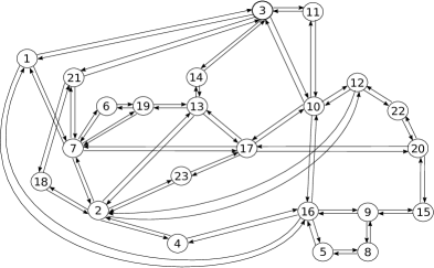
(d)

Figure 5.1. Bidirectional networks used in the simulations. A: A 3-by-3 Unidirectional network. B: A 3-by-3 bidirectional network. C: An 8-by-8 bidirectional network. D: The GÉANT network [40].

The ground truth data are generated as follows.

• Firstly, we find out all valid paths and OD trips for each network. For a given network $\mathcal{G}\left(\mathcal{N},\mathcal{L}\right)$, we find all the loop-free paths that involve at most $\tau_{\max}$ many links and denote the corresponding list by $\mathcal{L}_{{\rm path}}$. In this paper, we set $\tau_{\max}=4$. Using these paths, a list of valid OD trips is generated and denoted by $\mathcal{L}_{{\rm OD}}$. Based on $\mathcal{L}_{{\rm OD}}$, a list of origin nodes is constructed and denoted by $\mathcal{L}_{{\rm O}}$.

• Then, we randomly generate the assignment matrix for the O-flow model.

  • For each given origin node $o\in\mathcal{L}_{{\rm O}}$, all the OD pairs in $\mathcal{L}_{{\rm OD}}$ originating from $o$ are identified. Then a probability distribution over these OD pairs is randomly generated. This probability distribution defines the fractions of the O-flow $x_{o}$ for the involved OD flows $s_{od}$.

  • For each given OD pair $od\in\mathcal{L}_{{\rm OD}}$, all the paths in $\mathcal{L}_{{\rm path}}$ starting from the node $o$ and ending at the node $d$ are found. A probability distribution over these paths is randomly generated, which defines the fractions of the OD flow for the involved path flows $s_{\bm{p}}^{{\rm path}}$.

  • The assignment matrices related to both the OD flow and the O-flow models can be computed via Equations (3.6) and (3.7), respectively. Note that application of (3.7) requires the knowledge of OD flow assignment matrix $\bm{A}^{t}$, which further requires the knowledge of path flow assignment matrix according to (3.6). The previous sub-step is necessary.

• Finally, we randomly generate O-flows and compute the corresponding OD flows and link flows. We generate O-flows $\bm{x}^{t}$, $t=2-\tau_{\max},3-\tau_{\max},\cdots,n_{T}$, according to the transform domain sparsity model described in Section 4.2.2 (DCT transform is used). Based on the generated O-flows, the OD flows $\bm{s}^{t}$, $t=2-\tau_{\max},\cdots,n_{T}$, can be computed via (3.4), and the link flows $\bm{y}^{t}$, $t=1,2,\cdots,n_{T},$ can be evaluated via (3.2).

After generating the ground truth data, the test stage proceeds as follows. Given the link flows $\bm{y}^{t}$, the alternating minimization procedure described in Section 4 is used to estimate the O-flows $\{\hat{\bm{x}}^{t}\}$, $t=1,2,\cdots,n_{T}$, and the assignment matrices $\{\hat{\bm{P}}^{t}\}$, $t=1,2,\cdots,\tau_{\max}$.

The stopping criteria to quit the iterations include the following:

1. The maximum number of iterations is 5000.

2. Define the normalized mean square error by

   $${\rm NMSE}_{y}=\frac{\sum_{t}\left\|\hat{\bm{y}}^{t}-\bm{y}^{t}\right\|_{2}^{2}}{\sum_{t}\left\|\bm{y}^{t}\right\|_{2}^{2}}=\frac{\sum_{t}\left\|\hat{\bm{P}}^{t}*\hat{\bm{x}}^{t}-\bm{y}^{t}\right\|_{2}^{2}}{\sum_{t}\left\|\bm{y}^{t}\right\|_{2}^{2}}.$$

   The iteration stops when ${\rm NMSE}_{y}<10^{-5}$.

3. When the sparsity constraint is included, i.e., the formulation (4.11) is concerned, another stopping criterion is the speed of convergence. In particular, we define the decrease of the objective function at the $k$-th iteration as $\Delta=(\sum_{o=1}^{n_{n}}\left\|\bm{D}\bm{x}_{o}\right\|_{1})_{k-1}-(\sum_{o=1}^{n_{n}}\left\|\bm{D}\bm{x}_{o}\right\|_{1})_{k}$. The iteration stops when $\Delta<10^{-5}$.

After obtaining the estimated O-flows $\{\hat{\bm{x}}^{t}\}$ and the corresponding assignment matrices $\{\hat{\bm{P}}^{t}\}$, we compute the estimated OD flows $\{\hat{\bm{s}}^{t}\}$, $t=1,2,\cdots,n_{T}$, via Equation (3.4). The estimation performance is measured by the relative error in the estimated OD flows defined by

(5.1) $$E_{s_{od}}^{t}=\frac{\hat{s}_{od}^{t}-s_{od}^{t}}{s_{od}^{t}}.$$

When the value of $s_{od}^{t}$ is small, a small error in $\hat{s}_{od}^{t}$ may produce large relative error. If an approach performs well in relative error, it must be good.

In the simulations, the time horizon $n_{T}$ is chosen to not break the necessary condition in Theorem 10. The number of random trials is chosen according to the computation time (decided by the size of the problem as well as the convergence rate of Algorithm 1).

• The 3-by-3 unidirectional network in Figure 5.1a: $n_{T}=60$, and 10 random trials.

• The 3-by-3 bidirectional network in Figure 5.1b: $n_{T}=60$, and 100 random trials.

• The 8-by-8 bidirectional network in Figure 5.1c: $n_{T}=150$, and 10 random trials.

• The GÉANT network [40] in Figure 5.1d: $n_{T}=150$, and 10 random trials.

5.2. Blind Estimation Made Possible

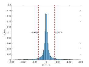
(a) The 3-by-3 bidirectional network

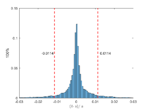
(b) The 8-by-8 bidirectional network

Figure 5.2. Histogram of relative errors: The 3-by-3 and 8-by-8 bidirectional networks

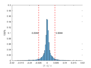
Figure 5.3. Histogram of relative errors: The GÉANT bidirectional network

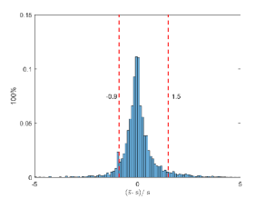
(a) Without transform domain sparsity assumption

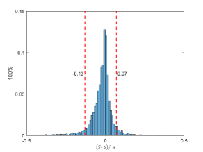
(b) With transform domain sparsity assumption

Figure 5.4. Histogram of relative error: The 3-by-3 unidirectional network.

Simulations demonstrate that for bidirectional networks our approach accurately recovers the OD flows without any prior information. The simulation results are presented in Figures 5.2 and 5.3 in the form of the histogram of relative errors (5.1). The x axis denotes the value of the relative error in the estimated OD flows. The y axis gives the percentage of OD flows for a given range of relative error. Each figure also contains two vertical dashed lines: accumulated 2.5% of the OD flows have (negative) relative error less than the value indicated by the left dashed line, accumulated 2.5% of the OD flows have relative error larger than the value indicated by the right dashed line, and accumulated 95% of the OD flows have the relative error between the values indicated by the dashed lines. Simulation results show that

• The 3-by-3 bidirectional network: Average relative error (in absolute value) is less than $0.1\%$. More than 95% of the estimated OD flows have relative errors in $\left[-0.66\%,0.72\%\right]$.

• The 8-by-8 bidirectional network: Average relative error (in absolute value) is less than $0.1\%$. More than 95% of the estimated OD flows have relative errors in $\left[-1.14\%,1.14\%\right]$.

• The GÉANT network: Average relative error (in absolute value) is less than $0.1\%$. More than 95% of the estimated OD flows have relative errors in $\left[-0.48\%,0.44\%\right]$.

The estimated OD flows are very accurate.

Simulation results for the 3-by-3 unidirectional network are presented in Figure 5.4. Figure 5.4a and Figure 5.4b show the histogram of relative errors before and after considering the transform domain sparsity, respectively:

• Before considering transform domain sparsity: Average relative error (in absolute value) is about $53\%$. More than 95% of the estimated OD flows have relative errors in $\left[-90\%,150\%\right]$.

• After considering transform domain sparsity: Average relative error (in absolute value) is about $3\%$. More than 95% of the estimated OD flows have relative errors in $\left[-13\%,7\%\right]$.

The results for the unidirectional network are less impressive compare to those for bidirectional networks. We suspect that this is due to the slow convergence of the Gauss-Seidel method, rather than our framework or the optimization formulation (4.11). Algorithm 1 terminates when either the number of iterations is already large or the improvement of the objective function in (4.11) is too small across adjacent iterations. However, we observe that, in all tested trials after the termination of the algorithm, the objective function still decreases along the line linking the output $\left\{\hat{\bm{P}}^{t}\right\}$ and the ground truth $\left\{\bm{P}^{t}\right\}$. This observation suggests that the output solution of Algorithm 1 is not a local minimal. An algorithm that solves (4.11) with faster convergence may significantly improve the estimation accuracy for unidirectional networks.

6. Conclusion and future work

To handle the ill-posedness of the OD flow estimation problem, this paper develops a linear forward model based on the O-flows. The dimension of the model is substantially reduced, and the OD flow information is preserved. Simulations demonstrate that for the first time blind estimation is possible. For bidirectional networks, the ground truth OD flows can be uniquely identified without any prior information. A necessary condition for the uniqueness of the solution is derived, which leads to the conclusion that unidirectional networks in general do not admit a unique solution under the O-flow model. Nevertheless, with the assumption of transform domain sparsity, the ground truth OD flows can be estimated in a reasonable accuracy.

As a starting point, this paper focuses on relatively simple settings. It will be beneficial to consider nonlinear traffic models, adapt the algorithm with different types of prior information, and experiment with large networks and real data. Furthermore, the algorithmic approach and Matlab implementation are not optimized, resulting in slow running speed which makes the current implementation not applicable to large network/data analysis. Efficient algorithm designs and implementations can benefit future research.

References

- [1] J. de Dios OrtÃozar and L. G. Willumsen, Modelling transport. John Wiley & Sons, 2011.
- [2] T. Toledo, H. Koutsopoulos, A. Davol, M. Ben-Akiva, W. Burghout, I. Andréasson, T. Johansson, and C. Lundin, “Calibration and validation of microscopic traffic simulation tools: Stockholm case study,” Transportation Research Record: Journal of the Transportation Research Board, no. 1831, pp. 65–75, 2003.
- [3] D. Bauer, G. Richter, J. Asamer, B. Heilmann, G. Lenz, and R. Kölbl, “Quasi-dynamic estimation of OD flows from traffic counts without prior OD matrix,” IEEE Transactions on Intelligent Transportation Systems, 2017.
- [4] L. G. Willumsen, “Estimation of an od matrix from traffic counts–A review.” 1978.
- [5] E. Cascetta, “Estimation of trip matrices from traffic counts and survey data: A generalized least squares estimator,” Transportation Research Part B: Methodological, vol. 18, no. 4, pp. 289–299, 1984.
- [6] C. Antoniou, R. Balakrishna, and H. N. Koutsopoulos, “A synthesis of emerging data collection technologies and their impact on traffic management applications,” European Transport Research Review, vol. 3, no. 3, pp. 139–148, 2011.
- [7] K. Parry and M. L. Hazelton, “Estimation of origin–destination matrices from link counts and sporadic routing data,” Transportation Research Part B: Methodological, vol. 46, no. 1, pp. 175–188, 2012.
- [8] P. Jin, M. Cebelak, F. Yang, J. Zhang, C. Walton, and B. Ran, “Location-based social networking data: Exploration into use of doubly constrained gravity model for origin-destination estimation,” Transportation Research Record: Journal of the Transportation Research Board, no. 2430, pp. 72–82, 2014.
- [9] L. Alexander, S. Jiang, M. Murga, and M. C. González, “Origin–destination trips by purpose and time of day inferred from mobile phone data,” Transportation research part c: emerging technologies, vol. 58, pp. 240–250, 2015.
- [10] L. Moreira-Matias, J. Gama, M. Ferreira, J. Mendes-Moreira, and L. Damas, “Time-evolving OD matrix estimation using high-speed gps data streams,” Expert systems with Applications, vol. 44, pp. 275–288, 2016.
- [11] X. Yang, Y. Lu, and W. Hao, “Origin-destination estimation using probe vehicle trajectory and link counts,” Journal of Advanced Transportation, vol. 2017, 2017.
- [12] H. Lo, N. Zhang, and W. Lam, “Decomposition algorithm for statistical estimation of OD matrix with random link choice proportions from traffic counts,” Transportation Research Part B: Methodological, vol. 33, no. 5, pp. 369–385, 1999.
- [13] H. Lo, N. Zhang, and W. H. Lam, “Estimation of an origin-destination matrix with random link choice proportions: A statistical approach,” Transportation Research Part B: Methodological, vol. 30, no. 4, pp. 309–324, 1996.
- [14] R. Frederix, F. Viti, and C. M. Tampere, “Dynamic origin–destination estimation in congested networks: Theoretical findings and implications in practice,” Transportmetrica A: Transport Science, vol. 9, no. 6, pp. 494–513, 2013.
- [15] J. Cao, S. V. Wiel, B. Yu, and Z. Zhu, “A scalable method for estimating network traffic matrices from link counts,” Preprint. Available at http://stat-www. berkeley. edu/binyu/publications. html, 2000.
- [16] H. Bar-Gera, “Traffic assignment by paired alternative segments,” Transportation Research Part B: Methodological, vol. 44, no. 8-9, pp. 1022–1046, 2010.
- [17] W. Shen and L. Wynter, “A new one-level convex optimization approach for estimating origin–destination demand,” Transportation Research Part B: Methodological, vol. 46, no. 10, pp. 1535–1555, 2012.
- [18] C.-C. Lu, X. Zhou, and K. Zhang, “Dynamic origin–destination demand flow estimation under congested traffic conditions,” Transportation Research Part C: Emerging Technologies, vol. 34, pp. 16–37, 2013.
- [19] R. Balakrishna, M. Ben-Akiva, and H. Koutsopoulos, “Offline calibration of dynamic traffic assignment: simultaneous demand-and-supply estimation,” Transportation Research Record: Journal of the Transportation Research Board, no. 2003, pp. 50–58, 2007.
- [20] R. Balakrishna and H. Koutsopoulos, “Incorporating within-day transitions in simultaneous offline estimation of dynamic origin-destination flows without assignment matrices,” Transportation Research Record: Journal of the Transportation Research Board, no. 2085, pp. 31–38, 2008.
- [21] L. Willumsen, “Simplified transport models based on traffic counts,” Transportation, vol. 10, no. 3, pp. 257–278, 1981.
- [22] M. G. Bell, “The estimation of origin-destination matrices by constrained generalised least squares,” Transportation Research Part B: Methodological, vol. 25, no. 1, pp. 13–22, 1991.
- [23] M. L. Hazelton, “Inference for origin–destination matrices: Estimation, prediction and reconstruction,” Transportation Research Part B: Methodological, vol. 35, no. 7, pp. 667–676, 2001.
- [24] M. Bierlaire and F. Crittin, “An efficient algorithm for real-time estimation and prediction of dynamic OD tables,” Operations Research, vol. 52, no. 1, pp. 116–127, 2004.
- [25] C. Xie, K. Kockelman, and S. Waller, “Maximum entropy method for subnetwork origin-destination trip matrix estimation,” Transportation Research Record: Journal of the Transportation Research Board, no. 2196, pp. 111–119, 2010.
- [26] W. H. Lam and H. Lo, “Estimation of origin-destination matrix from traffic counts: a comparison of entropy maximizing and information minimizing models,” Transportation Planning and Technology, vol. 16, no. 2, pp. 85–104, 1991.
- [27] E. Cascetta and S. Nguyen, “A unified framework for estimating or updating origin/destination matrices from traffic counts,” Transportation Research Part B: Methodological, vol. 22, no. 6, pp. 437–455, 1988.
- [28] C. Tebaldi and M. West, “Bayesian inference on network traffic using link count data,” Journal of the American Statistical Association, vol. 93, no. 442, pp. 557–573, 1998.
- [29] A. K. Menon, C. Cai, W. Wang, T. Wen, and F. Chen, “Fine-grained OD estimation with automated zoning and sparsity regularisation,” Transportation Research Part B: Methodological, vol. 80, pp. 150–172, 2015.
- [30] A. Tympakianaki, H. N. Koutsopoulos, and E. Jenelius, “Robust spsa algorithms for dynamic OD matrix estimation,” in 9th International Conference on Ambient Systems, Networks and Technologies May 8-11, 2018, Porto, Portugal, 2018.
- [31] K. Ashok and M. E. Ben-Akiva, “Alternative approaches for real-time estimation and prediction of time-dependent origin–destination flows,” Transportation Science, vol. 34, no. 1, pp. 21–36, 2000.
- [32] A. A. Prakash, R. Seshadri, C. Antoniou, F. C. Pereira, and M. E. Ben-Akiva, “Reducing the dimension of online calibration in dynamic traffic assignment systems,” Transportation Research Record: Journal of the Transportation Research Board, no. 2667, pp. 96–107, 2017.
- [33] E. Cipriani, M. Florian, M. Mahut, and M. Nigro, “A gradient approximation approach for adjusting temporal origin–destination matrices,” Transportation Research Part C: Emerging Technologies, vol. 19, no. 2, pp. 270–282, 2011.
- [34] T. Toledo and T. Kolechkina, “Estimation of dynamic origin–destination matrices using linear assignment matrix approximations,” IEEE Transactions on Intelligent Transportation Systems, vol. 14, no. 2, pp. 618–626, 2013.
- [35] G. Cantelmo, E. Cipriani, A. Gemma, and M. Nigro, “An adaptive bi-level gradient procedure for the estimation of dynamic traffic demand,” IEEE Transactions on Intelligent Transportation Systems, vol. 15, no. 3, pp. 1348–1361, 2014.
- [36] M. Bierlaire, “The total demand scale: a new measure of quality for static and dynamic origin-destination trip tables,” Transportation Research Part B: Methodological, vol. 36, no. 9, pp. 837 – 850, 2002.
- [37] M. A. Davenport and J. Romberg, “An overview of low-rank matrix recovery from incomplete observations,” IEEE Journal of Selected Topics in Signal Processing, vol. 10, no. 4, pp. 608–622, 2016.
- [38] R. Tibshirani, “Regression shrinkage and selection via the lasso,” Journal of the Royal Statistical Society. Series B (Methodological), pp. 267–288, 1996.
- [39] D. L. Donoho, “For most large underdetermined systems of linear equations the minimal -norm solution is also the sparsest solution,” Communications on Pure and Applied Mathematics, vol. 59, no. 6, pp. 797–829, 2006.
- [40] S. Uhlig, B. Quoitin, J. Lepropre, and S. Balon, “Providing public intradomain traffic matrices to the research community,” ACM SIGCOMM Computer Communication Review, vol. 36, no. 1, pp. 83–86, 2006.