Monodromy and chaos for condensed bosons in optical lattices

Abstract

We introduce a theory for the stability of a condensate in an optical lattice. We show that the understanding of the stability-to-ergodicity transition involves the fusion of monodromy and chaos theory. Specifically, the condensate can decay if a connected chaotic pathway to depletion is formed, which requires swap of seperatrices in phase-space.

I Introduction

Ergodicity, as opposed to Stability, is the threat that looms over the condensation of bosons in optical lattices. A major question of interest is whether an initial condensate is likely to be depleted. The simplest setup is the dimer, aka Bosonic Josephson Junction Chuchem et al. (2010); Albiez et al. (2005); Levy et al. (2007), where condensation in the upper orbital can become unstable if the interaction exceeds a critical value. A more challenging setup is a ring lattice Amico et al. (2014); Arwas and Cohen (2017); Paraoanu (2003); Hallwood et al. (2006); Gallemí et al. (2015), where the particles are condensed into an excited momentum orbital. If such flow-state is metastable, it can be regarded as a mesoscopic version of supefluidity. It has been realized that the theory for this superfluidity requires analysis that goes beyond the tradition framework of Landau and Bogoliubov, because the underlying dynamics is largely chaotic Kolovsky (2016); Arwas et al. (2015).

The structure of the classical phase-space is reflected in the quantum spectrum, and provides the key for quantum-chaos theory of mesoscopic superfluity. In the present work we highlight the essential ingredient for the crossover from stability to ergodicity. We consider the minimal setup: a 3 site ring. We show that the understanding of this transition involves the fusion of two major research themes: monodromy and chaos.

Monodromy.– The dynamics of an integrable (non-chaotic) system, for a given value of the conserved constants-of-motion, can be described by a set of action-angle variables, that parametrize a torus in phase space. In systems with monodromy, they cannot be defined globally: due to the non trivial topology of phase space, the action-angle variables cannot be identified in a continuous way in the parameter-space that is formed by the conserved quantities Duistermaat (1980); Cushman and Bates (1997). Accordingly, it is impossible to describe the quantum spectrum by a global set of good quantum numbers Cushman and Duistermaat (1988); Vũ Ngoc (1999). Rather, the good quantum numbers (quantized “actions”) that are implied by the EBK quantization scheme form a lattice that features a topological defect Zhilinskii (2006). Such Hamiltonian monodromy is found in many physical systems, such as the spherical Cushman and Duistermaat (1988); Efstathiou et al. (2004) and the swing-spring Cushman et al. (2004); Fitch et al. (2009) pendula, Spin-1 condensed bosons Lamacraft (2011), the Dicke model Kloc et al. (2017), and even the hydrogen atom Dullin and Waalkens (2018). A dynamical manifestation of monodromy in a classical system has been recently demonstrated Nerem et al. (2018).

Chaos.– The condensation of particles in a single orbital is a many-body coherent state. It can be represented in phase-space as a Gaussian-like distribution that is supported by a stationary point (SP). If this SP is the minimum of the energy landscape, it is known as Landau energetic stability, and leads, for a clean ring, to the Landau criterion for superfluidity. More generally one has to find the Bogoliubov excitations $\omega_{r}$ of condensate. If some of the frequencies become complex, the SP is considered to be unstable. What we have demonstrated in previous work Arwas et al. (2015); Arwas and Cohen (2017) was that this type of local stability analysis does not provide the required criteria for stability. Rather, in order to determine whether the system will ergodize, it is essential to study the global structure of phase-space, and to take into account the role of chaos.

Connectivity.– The major insight can be described schematically as follows. Let us regard the SP that supports the condensate as the origin of phase-space. And let us regard the region that supports the completely depleted states as the perimeter of phase-space. The crucial question is whether there is a dynamical pathway that leads from the origin to the perimeter. We have observed numerically in Arwas et al. (2015) that the formation of such pathway requires a swap of phase-space separatrices. But a theory for this swap transition has not been provided.

Outline.– For pedagogical purpose we first consider the stability question for the dimer. Then we go to the trimer and write its Hamiltonian as the sum of integrable part $\mathcal{H}^{(0)}$, and additional terms $\mathcal{H}^{(\pm)}$ that induce the chaos. An example for the classical and quantum spectra is presented in Fig.​​ 1. The spectra exhibit monodromy that we analyze in detail: the quantum monodromy is a reflection of the classical one. Then we explain how the spectrum is affected by changing a control parameter (detuning). In an hysteresis experiment Eckel et al. (2014) the detuning is determined by the rotation frequency of the device and the interaction strength between the bosons. We provide a geometrical explanation for the swap transition, and clarify the role of chaos in the de-stabilization of the condensate. In the summary section we point out the relevance of our study to the more general theme of thermalization in Bose-Hubbard chains.

II The Model

The Bose-Hubbard Hamiltonian (BHH) is a prototype model for cold atoms in optical lattices that has inspired state-of-the-art experiments Morsch and Oberthaler (2006); Bloch et al. (2008), and has been proposed as a platform for quantum simulations. It describes a system of $N$ bosons in $L$ sites. The ring geometry in particular has attracted attention for atomtronic circuits Amico et al. (2014). Taking into account that ${N}$ is constant of motion, the system has ${f=L{-}1}$ degrees of freedoms. The simplest configuration is the dimer ($L{=}2$), aka Bosonic Josephson Junction. Our main interest is in the minimal non-integrable configuration, which is the trimer ($L{=}3$). Below we briefly refer to the dimer Hamiltonian, and then turn to discuss the trimer Hamiltonian. Further technical details about the latter are provided in Appendix​ A.

II.1 The dimer

The Hamiltonian of the dimer is

$${}\mathcal{H}_{\text{dimer}}=-\frac{K}{2}\left({a}_{2}^{{\dagger}}{a}_{1}+{a}_{1}^{{\dagger}}{a}_{2}\right)+\frac{U}{2}\sum_{j=1}^{2}{a}_{j}^{{\dagger}}{a}_{j}^{{\dagger}}{a}_{j}{a}_{j}\ \ \ \ \$$ (1)

where $K$ is the hopping frequency, $U$ is the on-site interaction, The ${a}_{j}$ and ${a}_{j}^{{\dagger}}$ are the Bosonic annihilation and creation operators. The total number of particles $N=\sum_{j}{a}_{j}^{{\dagger}}{a}_{j}$ is a constant of motion.

It is convenient to switch to orbital representation. One defines annihilation and creation operators ${b}_{k}$ and ${b}_{k}^{{\dagger}}$, such that $b_{\pm}^{{\dagger}}=\frac{1}{\sqrt{2}}(a_{1}^{{\dagger}}\pm a_{2}^{{\dagger}})$ creates bosons in the lower and upper orbitals. For the purpose of semiclassical treatment we define action-angle variables via

$$b_{k}\ \ =\ \ \sqrt{n_{k}}\ e^{i\varphi_{k}}$$ (2)

After dropping an $N$ dependent constant the Hamiltonian takes the form

$${}\mathcal{H}_{\text{dimer}}(\tilde{\varphi},\tilde{n})\ =\ -\mathcal{E}\tilde{n}+\frac{U}{2}(N{-}\tilde{n})\,\tilde{n}\,[1+\cos(2\tilde{\varphi})]\ \$$ (3)

where $\tilde{n}=n_{+}$ is the occupation of the ($+$) orbital, and ${\mathcal{E}=K}$ is the detuning (energy difference between the orbitals). The angle ${\tilde{\varphi}=(\varphi_{+}-\varphi_{-})}$ serves as a conjugate coordinate. The phase space of this Hamiltonian has the topology of Bloch sphere. The Hamiltonian possesses two SPs that are located at ${\tilde{n}{=}0}$ and ${\tilde{n}{=}N}$, which are the North pole and the South poles of the Bloch sphere.

II.2 The trimer

The BHH for $L$ sites in a ring geometry is

$${}\mathcal{H}=\sum_{j=1}^{L}\left[\frac{U}{2}{a}_{j}^{{\dagger}}{a}_{j}^{{\dagger}}{a}_{j}{a}_{j}-\frac{K}{2}\left(\mathrm{e}^{i(\Phi/L)}{a}_{j{+}1}^{{\dagger}}{a}_{j}+\text{h.c.}\right)\right]\ \ \ \ \$$ (4)

where $j$ mod$(L)$ labels the sites of the ring, and other notations are as in the dimer case. The so-called Sagnac phase $\Phi$ is proportional to the rotation frequency of the device: it can be regarded as the Aharonov-Bohm flux that is associated with Coriolis field in the rotating frame Fetter (2009); Eckel et al. (2014).

It is convenient to switch to momentum representation. One defines annihilation and creation operators ${b}_{k}$ and ${b}_{k}^{{\dagger}}$, such that $b_{k}^{{\dagger}}=\frac{1}{\sqrt{L}}\sum_{j}\mathrm{e}^{ikj}a_{j}^{{\dagger}}$ creates bosons in the $k$-th momentum orbitals. Here we consider a 3-site ring that has 3 momentum orbitals labeled by their wavenumber ${k=0,1,2}$. Later we assume, without loss of generality, that the particles are initially condensed in the ${k=0}$ orbital. This is not necessarily the ground-state orbital, because we allow the possibility that the ring is in a rotating frame. After some time the condensate can be partially depleted such that the occupation is ${(N{-}n_{1}{-}n_{2},n_{1},n_{2})}$.

Since we have here an effectively 2 freedom system, it is convenient to define relative phases ${q_{1}=\varphi_{1}{-}\varphi_{0}}$ and ${q_{2}=\varphi_{2}{-}\varphi_{0}}$. Consequently the Hamiltonian can be written in terms of canonical coordinates as (Appendix​ A):

$${}\mathcal{H}(\varphi,n;\phi,M)=\mathcal{H}^{(0)}(\varphi,n;M)+\left[\mathcal{H}^{(+)}+\mathcal{H}^{(-)}\right]\ \$$ (5)

Here ${n=(n_{1}+n_{2})/2}$ and ${M=(n_{1}-n_{2})/2}$, while the conjugate angle variables are ${\varphi=q_{1}+q_{2}}$ and ${\phi=q_{1}-q_{2}}$. The first term $\mathcal{H}^{(0)}$ is an integrable piece of the Hamiltonian that has $M$ as an additional constant of motion:

$$\mathcal{H}^{(0)}(\varphi,n;M)\ =\ \mathcal{E}n+\mathcal{E}_{\perp}M-\frac{U}{3}M^{2}$$ (6)

$$\ \ +\frac{2U}{3}(N-2n)\left[\frac{3}{4}n+\sqrt{n^{2}-M^{2}}\cos(\varphi)\right]$$

where $U$ is the interaction between the bosons, while the detuning ${\mathcal{E}}$ determines the energy difference between the condensate (${n=0}$) and the depleted states (${n=N/2}$). If we linearized $\mathcal{H}$ with respect to the ${(n_{1},n_{2})}$ occupations, we would get the Bogoliubov approximation, which is Eq.​​ (LABEL:e2) without the third term ($M^{2}$), and with ${(N{-}2n)\approx N}$. The additional terms $\mathcal{H}^{(\pm)}$ induce resonances that spoil the integrability, and give rise to chaos.

$${}\mathcal{H}^{(\pm)}=\frac{2U}{3}\sqrt{(N{-}2n)(n{\pm}M)}(n{\mp}M)\cos\left(\frac{3\phi{\mp}\varphi}{2}\right)\ \ \ \$$ (7)

Note that classically the total number of particles $N$ can be removed from the Hamiltonian by a simple scaling of $n$ and $M$. But upon quantization $1/N$ effectively plays the role of $\hbar$. It follows that the coherent state that is formed by condensation of the particles into a single orbital is represented in phase-space by a Gaussian-like distribution of uncertainty width $1/N$. See for example Kolovsky (2016); Arwas et al. (2015). The significance of this $1/N$ scale for the analysis of instabilities due to non-linear resonances has been illuminated in Arwas and Cohen (2017).

\begin{overpic}[width=205.96883pt]{figBetaREVERSEsclUNN} \put(25.0,66.0){(a)} \end{overpic}

\begin{overpic}[width=205.96883pt]{fig1ascl} \put(25.0,64.0){(b)} \end{overpic}

Figure 1: Monodromy. The classical and quantum spectra of the Hamiltonian $\mathcal{H}^{(0)}$. This Hamiltonian has a constant of motion $M$, that describes the occupation imbalance of the ${k\neq 0}$ orbitals. In (a) each point represents an $(M,E)$ torus in phase space, and the points are color coded by the value of a classical phase ($\beta$) that characterizes the torus. In (b) each point represent an $\left|M,E\right\rangle$ eigenstate of $N=42$ particles, and the points are color coded by the expectation value of the variable $n$, which is the total occupation of the ${k\neq 0}$ orbitals. Yellow color (${n<N/8}$) indicates a nearly coherent condensate, while blue implies a depleted eigenstate. In both panels ${\mathcal{E}/NU\approx-1/4}$ and ${\mathcal{E}_{\perp}/NU\approx 1/2}$. The inset provides a zoom that demonstrates the monodromy: a topological defect in the lattice arrangement of the spectrum.

\begin{overpic}[trim=85.35826pt 0.0pt 71.13188pt 0.0pt,clip,width=57.23947pt]{fig1swapm8} \put(35.0,97.0){(a)} \end{overpic}

\begin{overpic}[trim=85.35826pt 0.0pt 71.13188pt 0.0pt,clip,width=56.37271pt]{fig1swapm2} \put(35.0,97.0){(b)} \end{overpic}

\begin{overpic}[trim=85.35826pt 0.0pt 71.13188pt 0.0pt,clip,width=56.37271pt]{fig1swapm03} \put(35.0,97.0){(c)} \end{overpic}

\begin{overpic}[trim=85.35826pt 0.0pt 71.13188pt 0.0pt,clip,width=56.37271pt]{fig1swap0} \put(35.0,97.0){(d)} \end{overpic}

\begin{overpic}[trim=85.35826pt 0.0pt 71.13188pt 0.0pt,clip,width=56.37271pt]{fig1swap03} \put(35.0,97.0){(e)} \end{overpic}

\begin{overpic}[trim=85.35826pt 0.0pt 71.13188pt 0.0pt,clip,width=56.37271pt]{fig1swap2} \put(35.0,97.0){(f)} \end{overpic}

\begin{overpic}[trim=85.35826pt 0.0pt 71.13188pt 0.0pt,clip,width=56.37271pt]{fig1swap8} \put(35.0,97.0){(g)} \end{overpic}

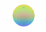
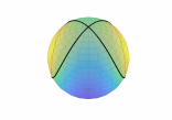
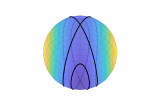
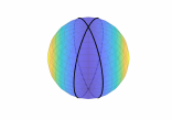
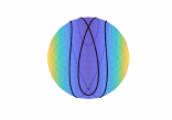
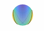
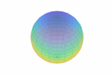
Figure 2: The geometry of the projected phase space. Top panels: the $(\varphi,n)$ disk. Bottom panels: the ${(\tilde{\varphi},\tilde{n})}$ Bloch-sphere. The detuning for (a-g) is ${\mathcal{E}/NU=-4/3,-1/3,-0.05,0,0.05,1/3,4/3}$. The color stands for the energy of $\mathcal{H}^{(0)}$, with $M=0$. Black lines indicate the separatrices that go through the SPs.

III Stability, Geometry, and Topology

Considering the dimer Hamiltonian Eq.​​ (1) it is well known that condensation at one orbital is always stable, while condensation at the second orbital becomes unstable if ${U}$ is large enough. This conclusion can be arrived by inspection of Eq.​​ (LABEL:e2): Without loss of generality let us assume that $U$ is positive (else the energy axis should be flipped); Considering condensation in the upper ($-$) orbital, we can regard $\tilde{n}\equiv n_{+}$ as the depletion coordinate; Then it follows, using the standard stability analysis of Appendix​ B, that the North pole (${\tilde{n}=0}$) becomes unstable if ${|\mathcal{E}|<NU}$.

Considering the trimer Hamiltonian, the supeficial impression is that $\mathcal{H}^{(0)}$ of Eq.​​ (LABEL:e2) is very similar to Eq.​​ (3) of the dimer: all we have to do is to rescale the occupation coordinate ${\tilde{n}=2n}$. However, the stability analysis of Appendix​ B shows that the regime-diagram of Eq.​​ (LABEL:e2) is in-fact more interesting: the condensate (${n=0}$) is unstable for ${-7NU/6<\mathcal{E}<NU/6}$, while the depleted state (${n=N/2}$) is unstable for ${-NU/6<\mathcal{E}<7NU/6}$. We will focus, in particular, on the the range ${|\mathcal{E}|<(1/6)NU}$, where both SPs become unstable. Note that $n=0$ necessary means that $M=0$, while $n=N/2$ is a SP for all $M$ values.

\begin{overpic}[trim=0.0pt 56.9055pt 0.0pt -56.9055pt,clip,width=65.04366pt]{cone1} \put(38.0,88.0){(a)} \end{overpic}

\begin{overpic}[trim=0.0pt 56.9055pt 0.0pt -56.9055pt,clip,width=65.04366pt]{cone4} \put(42.0,88.0){(b)} \end{overpic}

\begin{overpic}[trim=142.26378pt 0.0pt 142.26378pt 0.0pt,clip,width=65.04366pt]{pinchedtorus} \put(8.0,65.0){(c)} \end{overpic}

Figure 3: Phase space topology. The blue cone is an $M=0$ surface, that intersects with a surface of constant $E$. The existence of an additional coordinate ($\phi$) at each point is implicit. The intersection is a torus. Panel (a) is the typical case, while (b) corresponds to a pinched torus (see text). The latter is fully illustrated (with $\phi$) in panel (c).

Geometry.– The stability analysis reflect the algebraic side of the dynamics, but ignores the geometrical aspect. The phase space of the dimer is the Bloch sphere. All the ${(\tilde{\varphi},\tilde{n}{=}0)}$ points are in fact the same point, which can be regarded as the North pole of the sphere. Same applies to ${(\tilde{\varphi},\tilde{n}{=}N)}$ which can be regarded as the South pole of the sphere.

But for our 3 site ring Eq.​​ (LABEL:e2) the geometry of phase-space is different. The South pole, it is no longer a single point, because different $\varphi$ values indicate different points in phase space. So in fact we no longer have a Bloch-sphere, but rather we have a Bloch-disc. Another difference is that the angle is folded (${\varphi=2\tilde{\varphi}}$). The phase space structure, for different values of the detuning, is illustrated in Fig.​​ 2. The origin and perimeter of the $(\varphi,n)$ disk should be identified with the North and South poles of the ${(\tilde{\varphi},\tilde{n})}$ Bloch-sphere. The origin (${n=0}$), if unstable Fig.​​ 2(b-e), is the cusp on a folded separatrix of half-saddle topography. The perimeter of the disc is a spread SP. If the spread SP becomes unstable Fig.​​ 2(c-f), there is a separatrix that comes out from the perimeter in an angle ${\varphi_{\text{out}}}$, and comes back to it in an angle ${\varphi_{\text{in}}}$. Both the approach and the departure from the perimeter along the separatrix require an extremely long time. We emphasize again that from an algebraic point of view the dynamics is the same as if the perimeter were a single point on a Bloch-sphere. In the Bloch sphere each phase-space point is duplicated. Thanks to this duplication the separatrices that are associated with the SPs take the familiar figure-8 saddle shape, which is more illuminating for illustration purpose.

Topology.– So far we have discussed the one-freedom projected dynamics of ${(\varphi,n)}$. But now we have to remember that there is an additional degree of freedom ${(\phi,M)}$. We consider the dynamics that is generated by $\mathcal{H}^{(0)}$, where $M$ is a constant of motion, and the conjugate angle is doing circles with ${\dot{\phi}=\partial\mathcal{H}^{(0)}/\partial M}$. A trajectory that is generated by $\mathcal{H}^{(0)}$ covers a torus in phase space. A useful way for visualizing the tori is based on the $SU(1,1)$ symmetry Novaes (2004); Lamacraft (2011) of $\mathcal{H}^{(0)}$. The ${(\varphi,n)}$ dynamics is the intersection of constant $E$ and constant $M$ surfaces, see Fig.​​ 3 and Appendix​ C. In particular the ${M=0}$ surface is a cone, whose tip corresponds to ${n=0}$, while its outer boundary to ${n=N/2}$. If the intersection forms a closed loop, as in Fig.​​ 3a, the trajectory covers a torus in phase space. But if the trajectory goes through ${n=0}$, as in Fig.​​ 3b, we get a pinched torus, see Fig.​​ 3c. This is because the $\phi$-circle at ${n=0}$ has zero radius. This “zero radius” is explained as follows: if ${n=0}$ then necessarily ${n_{1}=n_{2}=0}$, hence all the ${(\varphi,\phi)}$ angles degenerate, representing a single phase-space point. In the projected dynamics Fig.​​ 2, the cusped trajectory which goes through $n=0$ (when unstable) is merely a projection of the pinched torus.

Definition of $\beta$.– Consider a trajectory that has a period $T$ in ${(\varphi,n)}$. For illustration this can be the trajectory that loops along the intersection in Fig.​​ 3a. Clearly, this trajectory is in general not a closed loop in the full phase space representation. Rather it winds on a two-dimensional torus. We define $\beta$ as the change in $\phi$ during time $T$. For a trajectory that passed through an unstable SP we have ${T\rightarrow\infty}$, and ${\beta}$ is ill-defined. In Fig.​​ 1a, we plot $\beta$ as a function of $M$ and $E$.

IV The swap transition

Recall that $\mathcal{E}$ is controlled experimentally by the rotation frequency of the device. Fig.​​ 2 shows the projected dynamics for different values of the detuning $\mathcal{E}$. In panels (c-e) both SPs are unstable, and we see how they swap as the detuning changes sign. At the transition the two separatrices coalesce, thus forming connection between the origin $n=0$ (which supports the condensate) and the perimeter $n=N/2$ (where the ${k{=}0}$ orbital is completely depleted).

On the Bloch-sphere, both North and South poles, when unstable, take the familiar 8-like shape. As we previously argued, this is due to the fact that the phase-space is duplicated, and that all the $\varphi$ values at the South pole are regarded as a single point. This physically unfaithful presentation possibly better reflects what do we mean by “swap of separatrices”. We note that the Poincare sections in Arwas et al. (2015), that had been presented before we gained proper understanding of the swap-transition, were physically unfaithful is the same sense.

Once the $\mathcal{H}^{(\pm)}$ terms are added, a connecting quasi-stochastic strip is formed, through which the initial state can decay. This is shown in Fig.​​ 5, where we plot a Poincare section of the full Hamiltonian Eq.​​ (5). One should note the subtle relation between the perspective of Fig.​​ 5 and that of Fig.​​ 2. A panel of the latter displays sections of ${M=0}$ tori that form a vertical subset in a Fig.​​ 1-type ${(M,E)}$ diagram, while a panel of Fig.​​ 5 displays sections of same $E$ trajectories that form a horizontal subset of such diagram. The pinched torus is contained in both subsets.

Away from the swap transition, the chaotic region around ${n=0}$ is bounded by the surviving Kolmogorov-Arnold-Moser (KAM) tori, forming a chaotic pond which is isolate from the perimeter region. Hence the depletion of the condensate is arrested. It is only in the vicinity of the swap transition that a connected chaotic pathway to depletion is formed. Thus, a local stability analysis of the SP using the standard Bogoliubov procedure does not provide the proper criterion for superflow metastability.

\begin{overpic}[trim=113.81102pt 28.45274pt 85.35826pt 14.22636pt,clip,width=65.04366pt]{sectionXm03run1} \put(4.0,92.0){(a)} \end{overpic}

\begin{overpic}[trim=113.81102pt 28.45274pt 85.35826pt 14.22636pt,clip,width=65.04366pt]{sectionX0run1} \put(4.0,92.0){(b)} \end{overpic}

\begin{overpic}[trim=113.81102pt 28.45274pt 85.35826pt 14.22636pt,clip,width=65.04366pt]{sectionX03run2} \put(4.0,92.0){(c)} \end{overpic}

\begin{overpic}[trim=113.81102pt 28.45274pt 85.35826pt 14.22636pt,clip,width=65.04366pt]{sectionXm03run2} \put(4.0,92.0){(d)} \end{overpic}

\begin{overpic}[trim=113.81102pt 28.45274pt 85.35826pt 14.22636pt,clip,width=65.04366pt]{sectionX0run2} \put(4.0,92.0){(e)} \end{overpic}

\begin{overpic}[trim=113.81102pt 28.45274pt 85.35826pt 14.22636pt,clip,width=65.04366pt]{sectionX03run1} \put(4.0,92.0){(f)} \end{overpic}

Figure 4: Poincare sections. The dynamics of the full Hamiltonian Eq.​​ (5) projected to the $(\varphi,n)$ disk. All the trajectories are launched with the same energy as that of the condensate, and the section is chosen to be $q_{2}=0$. The left to right arrangement of the panels is by detuning ${\mathcal{E}/NU=-0.05,0,0.05}$, in one-to-one correspondence with Fig.​​ 2(c-e). In the upper panels the interaction strength is ${NU\sim 1}$, in units of the BHH hopping frequency K, while in the lower panels it is doubled, keeping $\mathcal{E}/NU$ fixed. The color-code (from yellow to blue) corresponds to the trajectory-averaged occupation $n$ (from $N/8$ to $N/2$).

\begin{overpic}[width=69.38078pt]{specm03eta100} \put(20.0,62.0){(a)} \end{overpic}

\begin{overpic}[width=69.38078pt]{spec0eta100} \put(20.0,62.0){(b)} \end{overpic}

\begin{overpic}[width=69.38078pt]{spec03eta100} \put(20.0,62.0){(c)} \end{overpic}

\begin{overpic}[width=69.38078pt]{specm03eta111fig1} \put(20.0,62.0){(d)} \end{overpic}

\begin{overpic}[width=69.38078pt]{spec0eta111fig1} \put(20.0,62.0){(e)} \end{overpic}

\begin{overpic}[width=69.38078pt]{spec03eta111fig1} \put(20.0,62.0){(f)} \end{overpic}

\begin{overpic}[width=69.38078pt]{specm03eta111fig2} \put(20.0,62.0){(g)} \end{overpic}

\begin{overpic}[width=69.38078pt]{spec0eta111fig2} \put(20.0,62.0){(h)} \end{overpic}

\begin{overpic}[width=69.38078pt]{spec03eta111fig2} \put(20.0,62.0){(i)} \end{overpic}

Figure 5: The spectrum. The left to right arrangement of the panels is as in Fig.​​ 5. In the upper row we plot the spectrum of $\mathcal{H}^{(0)}$, while the two other rows provided the spectrum of $\mathcal{H}$ in one-to-one correspondence with Fig.​​ 5. All the spectra refer to ring with $N{=}42$ particles. The points are colored by the expectation value of $n$, with the same colorcode as in Fig.​​ 1b and Fig.​​ 5.

V Quantization

The classical structure of phase-space is reflected in the many-body spectrum. If chaos is ignored the eigenstates can be labeled by the good quantum numbers that are determined by the commuting operators ${M}$ and ${\mathcal{H}^{(0)}}$, as in Fig.​​ 1b. If we add the $\mathcal{H}^{(\pm)}$ terms we can still order the energies according to the expectation value ${\left\langle M\right\rangle}$. Several examples are provided in Fig.​​ 5. For presentation purpose, the perimeter energy ${E_{x}(M)}$, which corresponds to maximum depleted state (${n=N/2}$), is taken as the reference. Fig.​​ 7 of Appendix​ D provides spectra for the whole range of the detuning parameter, corresponding to the phase space plots of Fig.​​ 2.

From a semiclassical perspective, if we ignore the chaos, each point can be associated with an EBK torus Appendix​ E. Namely, the “good quantum numbers” are quantized values of the action variables. The lattice arrangement of the energies in Fig.​​ 1b reflects the way that the tori are embedded in phase-space, while the chaos, once added, blurs it locally, see Fig.​​ 5. This lattice arrangement is supported by a classical skeleton that is formed by a pinched torus (marked by a red dot), and an ${E=E_{x}(M)}$ separatrix. At the vicinity of the separatrix the spectrum is dense, reflecting that the frequency of the motion goes to zero. Irrespective of that, the quantum spectrum has a topological defect that is described by a monodromy (to be further discussed below). This monodromy reflects the presence of the pinched torus. The sequence of panels in Fig.​​ 5 shows how the swap transition is reflected in the quantum spectrum. This transition happens as the red dot, which corresponds to the pinched torus, crosses the $E=E_{x}$ separatrix line. We see how the yellow condensation region is diminished at the transition.

VI Monodromy calculation

The concept of monodromy is pedagogically summarized in Appendix​ E. For our model system, in the absence of chaos, we have in involution the generators ${H_{1}=\mathcal{H}^{(0)}}$ and ${H_{2}=M}$. The trajectories that are generated for a given $E$ and $M$ form a torus. Any point on the torus is accessible by generating a walk of duration ${(t_{1},t_{2})}$. Consider the projected dynamics in ${(\varphi,n)}$. A given trajectory has a period $T$, but in the full phase-space it is, in general, not periodic, because $\phi$ has advanced some distance $\beta$. It follows that in order to get a periodic walk on the torus, the ${t_{1}=T}$ evolution that is generated by ${H_{1}}$, should be followed by a ${t_{2}=-\beta}$ evolution that is generated by ${H_{2}}$. The so called rotation angle, $\beta$, characterizes the torus, and is imaged in Fig.​​ 1a. Note that a ${t_{2}=4\pi}$ evolution that is generated by ${H_{2}=M}$ is a periodic trajectory in phase space, because it does not affect the ${(\varphi,n)}$ degree of freedom. We conclude that the set of periodic walks forms a lattice that can be spanned by the basis vectors

$${}\vec{\tau}_{a} = (T,-\beta)$$ (8)

$$\vec{\tau}_{b} = (0,4\pi)$$ (9)

A remark is in order regarding the determination of the $4\pi$ in Eq.​​ (9). It should be clear that the original phases ${(\varphi_{0},\varphi_{1},\varphi_{2})}$ are defined ${\mod(2\pi)}$. Next we define the coordinates ${q_{1}=\varphi_{1}-\varphi_{0}}$ and ${q_{2}=\varphi_{2}-\varphi_{0}}$, and the alternate coordinates ${\phi=q_{1}-q_{2}}$ and ${\varphi=q_{1}+q_{2}}$. If the alternate coordinates are regarded as ${\mod(2\pi)}$ angles, it follows that each ${(\varphi,\phi)}$ represent two points in $q$ space, and each ${(\varphi,n)}$ in our sections is the projection of a $4\pi$ circle. Consider a trajectory that is generated using ${H_{2}=M}$. In the ${(\varphi_{1},\varphi_{2})}$ torus it will have a constant ${\varphi}$. You will have to run ${t}$ a ${4\pi}$ interval in order to get back to the starting point.

Quantum to classical duality.– Let us now go back to Fig.​​ 1a, where we plot $\beta$ as a function of $M$ and $E$. One can immediately spot the location of the pinched torus $(M,E)=0$, around which $\beta$ has ${4\pi}$ variation. Hence, after a parametric loop, we get the mapping ${\vec{\tau}_{a}\mapsto\vec{\tau}_{a}-\vec{\tau}_{b}}$ while ${\vec{\tau}_{b}}$ remains the same. Such non-trivial mapping is the hallmark of monodromy Duistermaat (1980); Cushman and Bates (1997). Upon EBK quantization monodromy in the spectrum is implied, see Appendix​ E. This is demonstrated in the inset of Fig.​​ 1b. Namely, transporting an elementary unit cell (spanned by two basis vectors) around the pinched torus in the $(M,E)$ spectrum, we end up with a different unit cell.

In Fig.​​ 1a the detuning was chosen such that the SP at $n=N/2$ is stable. Contrary for that, in Fig.​​ 5 the detuning is such that the SP is at the vicinity of a swap transition. Consequently the spectrum is divided into two regions by the separatrix line, and only the region with the pinched torus exhibits the non-trivial monodromy. At the swap transition the pinched torus and hence the non-trivial monodromy is relocated to the other region. In the special case of $\mathcal{E}=0$, the pinched torus merges with the separatrix line, leaving both regions with a trivial monodromy.

VII Summary

Several themes combine is the study of superflow metastability. There is a monodromy that is associated with the SP that supports the condensate; and a separatrix that is associated with an SP that folds all the depleted states. The two SPs determine the skeleton of phase space. By duality it is also the skeleton for the many-body quantum spectrum (via EBK quantization). In the Bloch sphere representation (Fig.​​ 2) the two SPs look-alike, but this is in fact wrong and misleading. The topological distinction between the central SP and the peripheral SP becomes conspicuous once we look on the quantum spectrum where the central SP-monodromy appears as a topological defect that reflects the existence of a pinched torus, while the depleted peripheral states form a dense line in ${(M,E)}$ space.

By itself the above described skeleton is not enough for the understanding of BEC metastability or its absence. The theoretical narrative requires the fusion of chaos into the story. If the rotation frequency of the device is adjusted (which controls the detuning between the central SP and the peripheral separatrix), a stochastic pathway is formed at the “swap transition”, leading to the depletion of the condensate, and the decay of the superflow. In the dual quantum picture chaos blurs the ordered spectrum. Away from the swap transition the topological aspect remains robust , but at the swap transition eigenstates get-mixed and become ergodic within the stochastic region.

The analysis that we have introduced is specifically relevant for future hysteresis-type experiments Eckel et al. (2014) with ring lattice circuits Bell et al. (2016); Aidelsburger et al. (2017). Furthermore, the trimer is not only the minimal model for ergodization due to chaos, it is also the minimal configuration for thermalization trm , and serves as the building-block for progressive thermalization of large arrays basko ; henning . Finally, it should be recognized that the theme of metastability is of general interest for mathematical-physics studies of high dimensional chaos, irrespective of specific application.

Acknowledgements.– This research was supported by the Israel Science Foundation (Grant No.283/18)

Appendix A The Trimer Hamiltonian

For a clean $L$-site ring lattice we define momentum orbitals whose wavenumbers are $k=(2\pi/L)\times\text{integer}$. Consequently the BHH takes the form

$${}\mathcal{H}\ \ =\ \ \sum_{k}\epsilon_{k}b_{k}^{{\dagger}}b_{k}\ +\ \frac{U}{2L}\sum^{\prime}b_{k_{4}}^{{\dagger}}b_{k_{3}}^{{\dagger}}b_{k_{2}}b_{k_{1}}$$ (10)

where the constraint ${k_{1}{+}k_{2}{+}k_{3}{+}k_{4}=0}$ mod($2\pi$) is indicate by the prime, and ${\epsilon_{k}=-K\cos(k-\Phi/L)}$ are the single particle energies. Later we assume, without loss of generality, that the particles are initially condensed in the ${k=0}$ orbital. This is not necessarily the ground-state orbital, because we keep $\Phi$ as a free parameter. Note that below and in the main text we optionally use $k$ as a dummy index to label the momentum orbitals.

For the ${L=3}$ site ring we have

$$\mathcal{H}\ \ = \ \ \sum_{k=0,1,2}\epsilon_{k}n_{k}\ +\ \frac{U}{6}\sum_{k}n_{k}^{2}\ +\ \frac{U}{3}\sum_{k^{\prime}\neq k}n_{k^{\prime}}n_{k}$$

$$+ \frac{U}{3}\sum_{k^{\prime\prime}\neq k^{\prime}\neq k}\left[n_{k^{\prime}}n_{k^{\prime\prime}}\right]^{1/2}\ n_{k}\ \cos\left(\varphi_{k^{\prime\prime}}+\varphi_{k^{\prime}}-2\varphi_{k}\right)$$

We define ${q_{1}=\varphi_{1}-\varphi_{0}}$ and ${q_{2}=\varphi_{2}-\varphi_{0}}$ where the subscripts refers to ${k_{1,2}=\pm(2\pi/3)}$. Using the notation ${\mathcal{E}_{k}=(\epsilon_{k}-\epsilon_{0})+(1/3)NU}$ we get Eq.​​ (5) with

$$\mathcal{H}^{(0)}\ = \ \mathcal{E}_{1}n_{1}+\mathcal{E}_{2}n_{2}\ -\ \frac{U}{3}\left[n_{1}^{2}+n_{2}^{2}+n_{1}n_{2}\right]$$ (12)

$$+ \ \frac{2U}{3}(N{-}n_{1}{-}n_{2})\sqrt{n_{1}n_{2}}\cos\left(q_{1}+q_{2}\right)$$

and

$${}\mathcal{H}^{(+)}\ =\ \frac{2U}{3}\sqrt{(N{-}n_{1}{-}n_{2})n_{1}}\ n_{2}\cos\left(q_{1}-2q_{2}\right)$$ (13)

while $\mathcal{H}^{(-)}$ is obtained by swapping the indices (${1\leftrightarrow 2}$). In fact it is more convenient to use the coordinates

$${}\phi[\text{mod}(4\pi)] \ =\ q_{1}-q_{2}\ =\ \varphi_{1}-\varphi_{2}$$

$$\varphi[\text{mod}(2\pi)] \ =\ q_{1}+q_{2}\ =\ \varphi_{1}+\varphi_{2}-2\varphi_{0}$$ (14)

and the conjugate coordinates

$$M \ =\ \frac{1}{2}(n_{1}-n_{2})\ \ \in\left[-\frac{N}{2},\frac{N}{2}\right]$$ (15)

$$n \ =\ \frac{1}{2}(n_{1}+n_{2})\ \ \in\left[|M|,\frac{N}{2}\right]$$ (16)

Then the Hamiltonian takes the form of Eq.​​ (5) with Eq.​​ (LABEL:e2) and Eq.​​ (7), where the detuning is ${\mathcal{E}=\mathcal{E}_{1}+\mathcal{E}_{2}-(1/2)NU}$, and ${\mathcal{E}_{\perp}=\mathcal{E}_{1}-\mathcal{E}_{2}}$.

Appendix B SPs and seperatrices

Consider a phase-space that is described by ${\varphi,n}$. We shall distinguish between rotor geometry for which the ${n=0}$ points are distinct, and oscillator geometry for which all the ${n=0}$ points are identified as one point. The algebraic treatment is the same, but the physical interpretation is different.

Regular point.– As an appetizer consider the Hamiltonian

$${}H\ \ =\ \ \sqrt{2n}\sin(\varphi)$$ (17)

It looks singular at ${n=0}$, but in fact it is completely smooth there. Regarded as an oscillator it is canonically equivalent to ${H=p}$ that generates translations. Similar observation applies to the non-interacting dimer Hamiltonian ${H=(1/2)(a_{2}^{{\dagger}}a_{1}+\text{h.c.})}$, which in action angle variables takes the form

$$H\ \ =\ \ \sqrt{\left(\frac{N}{2}-n\right)\left(\frac{N}{2}+n\right)}\ \cos(\varphi)$$ (18)

Here both the North and the South poles of the Bloch sphere (${n=\pm N/2}$) are regular phase-space points, neither SP nor singular.

Stationary point.– Consider the standard quadratic Hamiltonian ${H=(1/2)[ap^{2}+bx^{2}]}$. In polar canonical coordinates it is

$${}H\ \ =\ \ \left[A+B\cos(2\varphi)\right]\ n$$ (19)

with ${A=(a+b)}$ and ${B=(a-b)}$. If ${ab>0}$, equivalently ${|A|>|B|}$, the origin (${n=0}$) is an elliptic SP that is circled by trajectories that have the frequency

$${}\omega\ =\ \sqrt{ab}\ =\ \sqrt{A^{2}-B^{2}}$$ (20)

Otherwise the origin becomes an unstable hyperbolic SP. In the latter case there is an 8-like separatrix that goes through the origin: there are two ingoing directions and two outgoing directions. The approach to the SP along the separatrix, and its departure, is an infinitely slow motion. The SPs of the dimer Eq.​​ (3) are described locally by the above Hamiltonian.

Folded SP.– Consider the dimer Hamiltonian Eq.​​ (3) with $2\tilde{\varphi}$ replaced by $\varphi$. Here the dynamics is the same from algebraic perspective, but the global geometry is different. It is a folded version of the dimer Hamiltonian. In the hyperbolic case the vicinity of the SP can be described as “half saddle”. From local dynamics point of view the equations of motion are identical, but here the separatrix has only one outgoing direction and only one ingoing direction.

Spread SP.– Consider Eq.​​ (19), but assume that we are dealing with rotor geometry. From local dynamics point of view the equations of motion are still identical, but now the arrival point (say ${\varphi_{in}}$) and the departure point (say ${\varphi_{out}}$) are not the same point.

Stability analysis.– Consider the Hamiltonian of Eq.​​ (LABEL:e2) with ${M=0}$. The origin (${n=0}$) is a folded SP. It is elliptic or hyperfolic depending on the detuning. Locally the Hamiltonian looks like Eq.​​ (19) with

$$A=\mathcal{E}+\frac{NU}{2},\ \ \ \ \ B=\frac{2NU}{3}$$ (21)

$$\text{SP unstable for}\ \ -\frac{7NU}{6}<\mathcal{E}<\frac{NU}{6}$$ (22)

In the regime where the SP is stable the $\omega$ of Eq.​​ (20) reflects the frequency of the Bogoliubov excitations Arwas et al. (2015). In the hyperbolic case we have a separatrix that goes through the origin.

For the same Hamiltonian, the perimeter (${n=N/2}$) is a spread SP. For the purpose of stability analysis we can identify the points along the perimeter as a single point of a Bloch sphere. Setting $\tilde{n}=N-2n$ the Hamiltonian looks like Eq.​​ (19) with

$$A=-\frac{\mathcal{E}}{2}+\frac{NU}{4},\ \ \ \ \ B=\frac{NU}{3}$$ (23)

$$\text{SP unstable for}\ \ -\frac{NU}{6}<\mathcal{E}<\frac{7NU}{6}$$ (24)

In the hyperbolic case we have a separatrix that meets the perimeter at one point and departs in a different point. Combining with Eq.​​ (22) we see that both SPs are unstable if ${|\mathcal{E}|<(1/6)NU}$. In the latter case we have two seperatrices. The separatrices swap as we go through ${\mathcal{E}=0}$, see Fig.​​ 1.

The case of nonzero $M$.– For the same Hamiltonian Eq.​​ (LABEL:e2) with ${M\neq 0}$, the points along the inner boundary ${n=M}$ are distinct. So we cannot regard them as a single point. Close to this inner boundary we have ${H\sim\sqrt{\tilde{n}}\cos(\varphi)}$, with ${\tilde{n}=n-M}$. This is a non-singular Hamiltonian, essentially the same as Eq.​​ (17), that generates regular flow. It follows that the inner boundary is not special from a dynamical point of view: it can be regarded as spread regular point, it is not an SP, and there is no separatrix there.

The stability of the perimeter is determined as in Eq.​​ (24), but with $B$ multiplied by $\sqrt{1-(2M/N)}$. Therefore, for sufficiently large $M$ we always have ${|A|>|B|}$ and the perimeter is stable.

\begin{overpic}[width=65.04366pt]{cone1} \put(22.0,95.0){(a)} \end{overpic}

\begin{overpic}[width=65.04366pt]{cone2} \put(22.0,99.0){(b)} \end{overpic}

\begin{overpic}[width=65.04366pt]{cone3} \put(22.0,99.0){(c)} \end{overpic}

\begin{overpic}[width=65.04366pt]{cone4} \put(22.0,95.0){(d)} \end{overpic}

\begin{overpic}[width=65.04366pt]{cone5} \put(22.0,95.0){(e)} \end{overpic}

\begin{overpic}[width=65.04366pt]{cone6} \put(22.0,90.0){(f)} \end{overpic}

Figure 6: Several examples of the reduced phase-space in the $(K_{x},K_{y},K_{z})$ coordinates (the symmetry axis is $K_{z}$). The blue cone (a,c-f) is the surface of constant $M=0$ while the blue hyperbole (b) is the surface of constant $M=0.15N$. The remaining surfaces correspond to a constant $E$. The intersection of constant $M$ and $E$ surfaces (highlighted in black) is a trajectory in the reduced $(\varphi,n)$ space, and provides a useful way of visualizing the phase space tori (see text).

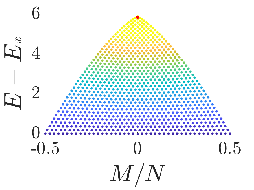
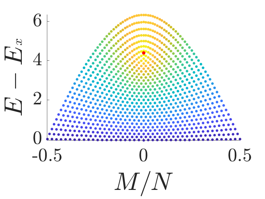
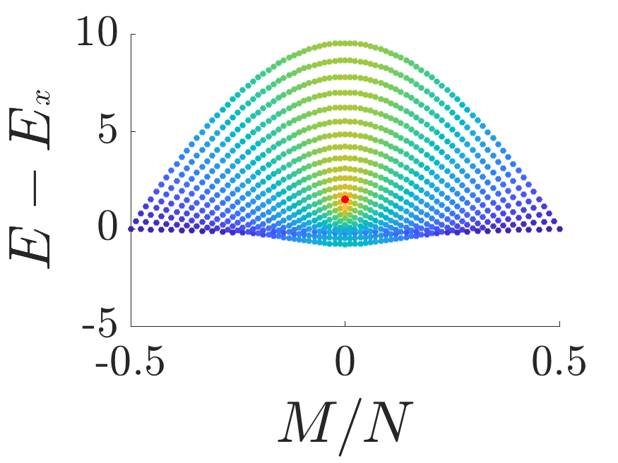
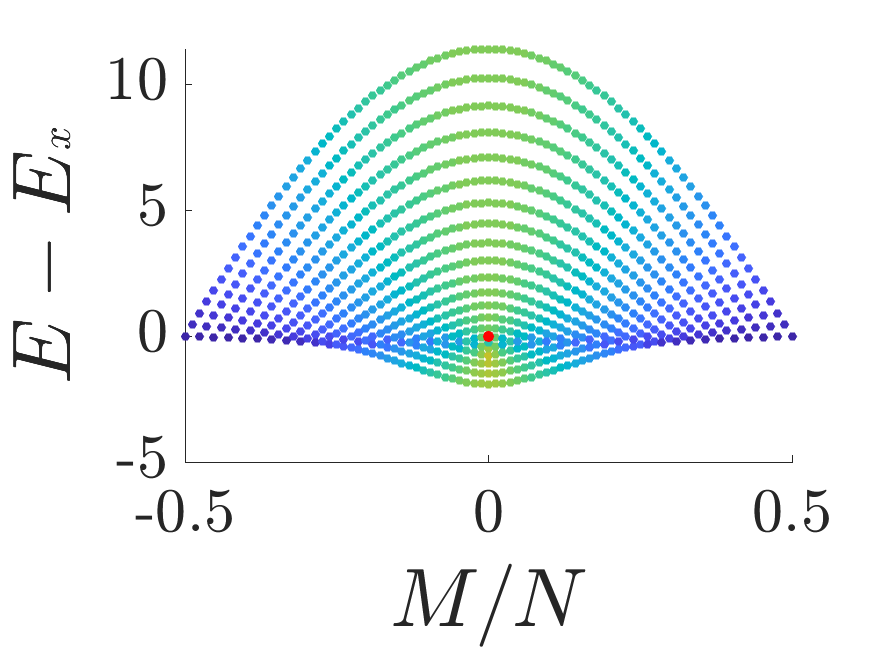
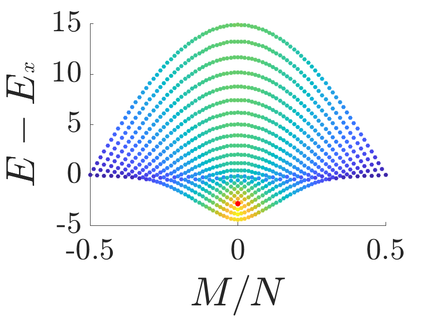
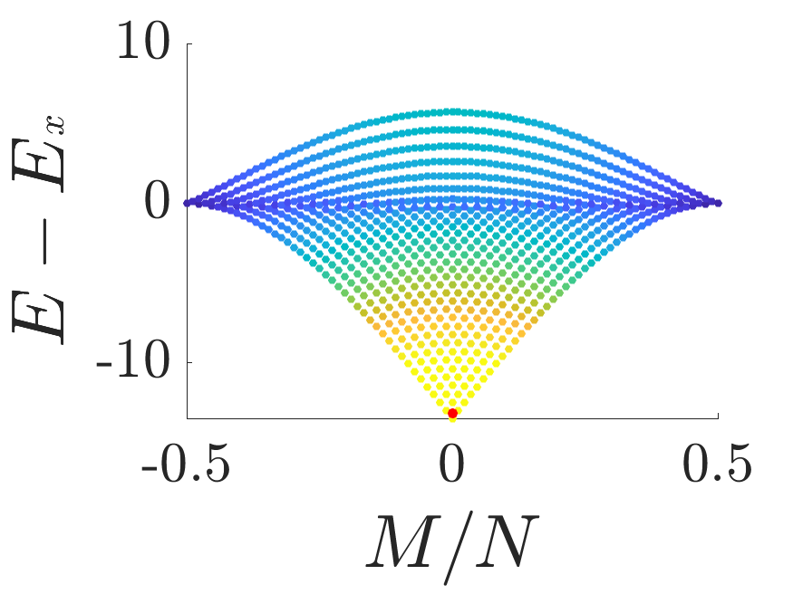
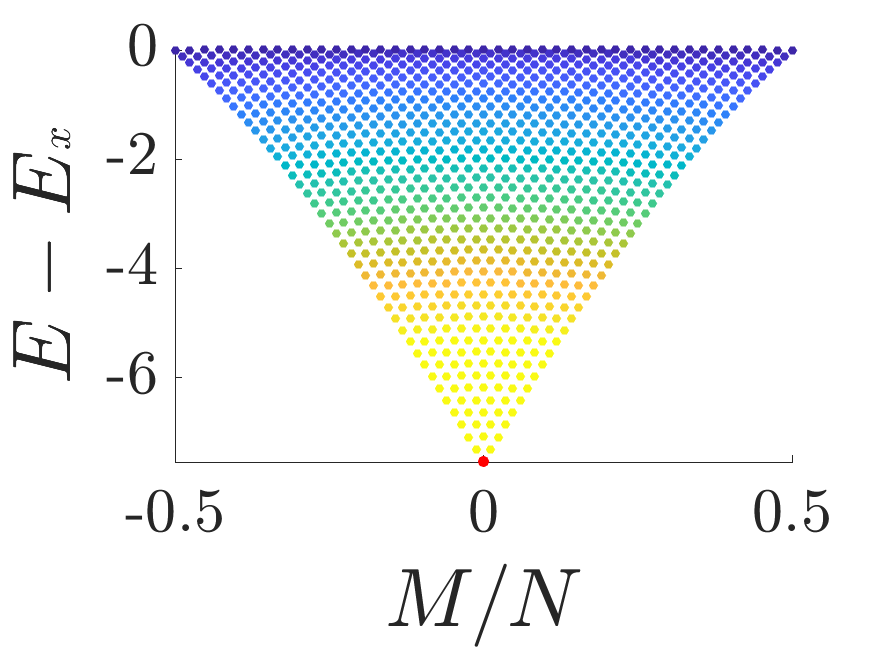
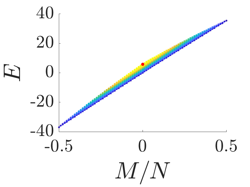
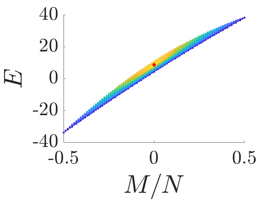
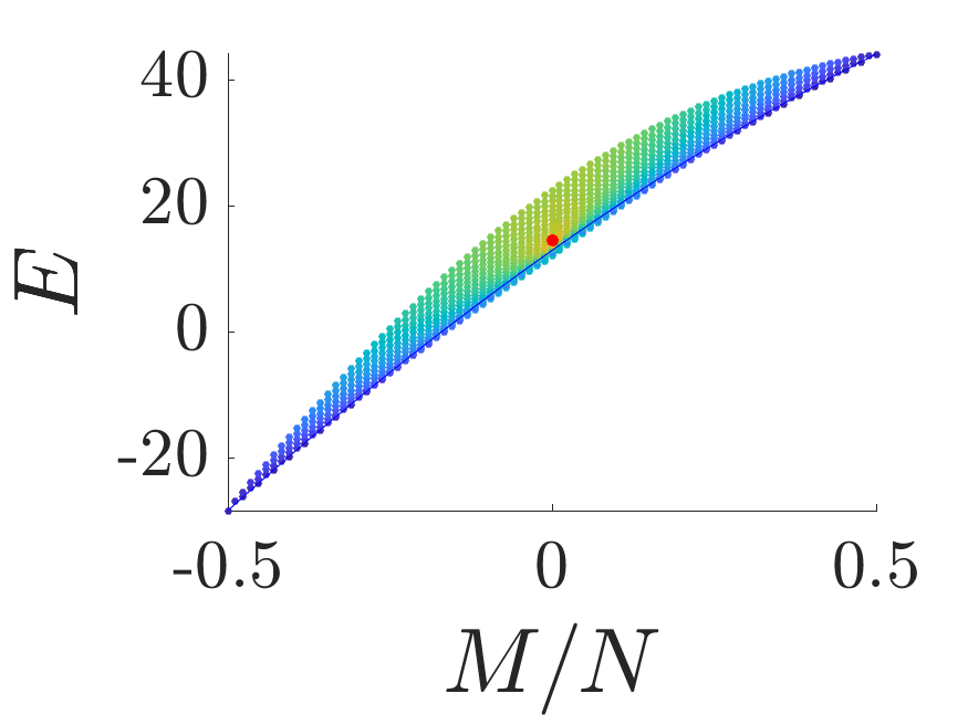
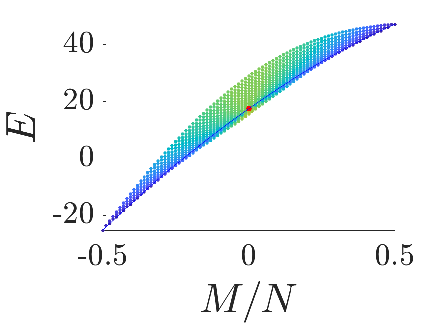
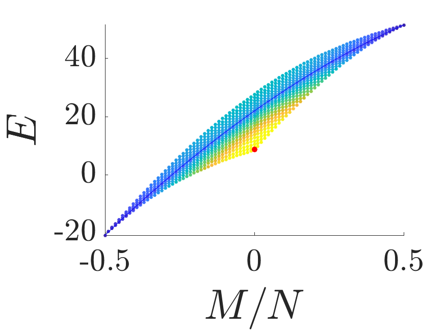
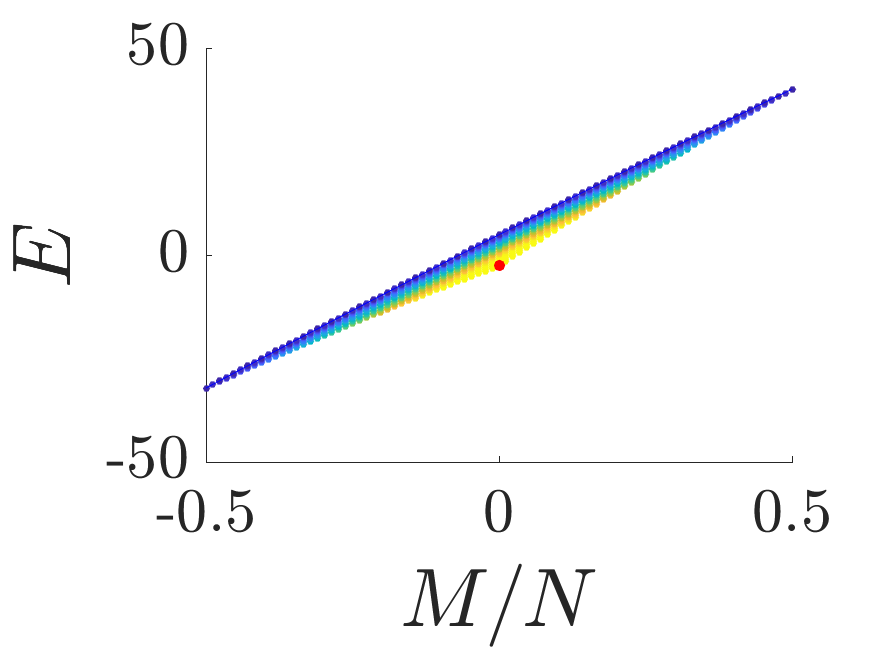
Figure 7: The spectrum. The top row panels are the spectrum of $\mathcal{H}^{(0)}$ with the same $\mathcal{E}/NU$ values as in Fig.​​ 2. In the bottom row the same spectra is plotted, but without subtracting the separatrix energy. The interaction strength from left to right is $NU\approx 0.2,0.6,1.4,1.9,2.7,1.9,0.3$ in units of the BHH hopping frequency $K$. Note that for the top row panels, different $NU$ values will produce the same plot and only scale the $E-E_{x}$ axis. Note that the energy here differs by a constant from Fig.​​ 1(b).

Appendix C Conical intersection perspective

A useful way for visualizing the phase space tori is based on the $SU(1,1)$ symmetry Novaes (2004); Lamacraft (2011) of $\mathcal{H}^{(0)}$. For that we express the two conserved quantities, namely the energy $E$ and the constant of motion $M$, in terms of the group generators. We start by introducing:

$$K_{z}=n+\frac{1}{2}\ \ \ ,\ \ \ K_{+}=a_{1}^{\dagger}a_{2}^{\dagger}\ \ \ ,\ \ \ K_{-}=a_{1}a_{2}$$ (25)

which is a realization of the $SU(1,1)$ group, satisfying the algebra:

$$[K_{z},K_{\pm}]=\pm K_{\pm}\ \ \ ,\ \ \ [K_{+},K_{-}]=-2K_{z}$$ (26)

The Casimir operator of the group, which commutes with all the generators, is:

$$C\ =\ K_{z}^{2}-K_{x}^{2}-K_{y}^{2}$$ (27)

where $K_{x}$ and $K_{y}$ are given by $K_{\pm}=K_{x}\pm iK_{y}$. In the semiclassical treatment we have:

$$K_{x} \ \sim\ \sqrt{n_{1}n_{2}}\cos\varphi\ \ \in\left[-\Delta,\Delta\right]$$ (28)

$$K_{y} \ \sim\ \sqrt{n_{1}n_{2}}\sin\varphi\ \ \in\left[-\Delta,\Delta\right]$$ (29)

$$K_{z} \ \sim\ n\ \ \in\left[|M|,\frac{N}{2}\right]$$ (30)

where $\Delta=\sqrt{(N/2)^{2}-M^{2}}$. The Hamiltonian can be written in terms of the generators as:

$$\mathcal{H}^{(0)}\ = \ \mathcal{E}K_{z}+\mathcal{E}_{\perp}M-\frac{U}{3}M^{2}$$

$$+ \ \frac{2U}{3}(N-2K_{z})\left[\frac{3}{4}K_{z}+K_{x}\right]$$

As for the constant of motion $M$, we have $M^{2}=C$. In Fig.​​ 6 we plot several examples for the $M^{2}$ and $\mathcal{H}^{(0)}=E$ surfaces in the $(K_{x},K_{y},K_{z})$ space. For $M=0$ Eq.​​ (27) defines a cone whose tip corresponds to ${n=0}$, while its outer boundary to ${n=N/2}$. For for a constant $M\neq 0$ Eq.​​ (27) defines an hyperboloid whose base corresponds to ${n=|M|}$, while its outer boundary to ${n=N/2}$.

The intersection between the $E$ and $M^{2}$ surfaces is a trajectory in the reduced $(\varphi,n)$ phase space. In the full phase space, we also have the phase $\phi$, which dynamically changes as ${\dot{\phi}=\partial\mathcal{H}^{(0)}/\partial M}$. If the intersection between the surfaces forms a closed loop, as in Fig.​​ 6(a,b), the dynamics in the full $(\varphi,\phi,n,M)$ phase-space covers a 2-torus (which is, of course, the typical case in an integrable 2 DOF system). When the two surfaces tangent, as in Fig.​​ 6(b), the trajectory is a fixed point in the $(\varphi,n)$ space, and a circle in the full phase space.

Trajectories that pass through $n=0$ should be addressed with more caution. As explained in the main text, the tip of the cone does not correspond to a $\phi$ circle, but to a single point. This is because $n=0$ means $n_{1}=n_{2}=0$ so that $\phi$ is degenerate. When the $n=0$ SP is stable, the energy surface is tangent to the tip of the cone, as in Fig.​​ 6(c), hence the trajectory is a single point in phase space. When unstable, the intersection forms a cusped circle, see Fig.​​ 6(d), representing a pinched torus, i.e. a torus with one of its $\phi$ circles shrinks to a point.

Trajectories that pass through $n=N/2$ are special too. When the $n=N/2$ SP is stable, as in Fig.​​ 6(c), the intersection is the entire outer circle of the cone, reflecting the fact that it is a spread SP. When unstable, see Fig.​​ 6(e), a separatrix trajectory is formed, which meets the $n=N/2$ circle at two points, corresponding to ${\varphi_{\text{in}}}$ and ${\varphi_{\text{out}}}$. At the swap transition, the two SPs are connected, i.e. the cusped circle of $n=0$ merged with the separatrix trajectory of $n=N/2$, as shown in Fig.​​ 6(f).

Appendix D Gallery

Here we provide additional plots of the spectra for the whole range of the detuning parameter. Fig.​​ 7 is an extended version of Fig.​​ 5 and corresponds to Fig.​​ 2.

Appendix E Hamiltonian Monondromy

Consider generators ${(H_{1},H_{2})}$ in involution, i.e. that commute with each other. The generated trajectories are moving on an energy surface labeled ${(E_{1},E_{2})}$. A walk consists of ${t_{1}}$ evolution using ${H_{1}}$, and ${t_{2}}$ evolution using ${H_{2}}$. The involution implies that the walks are commutative. Accordingly the parameterization of a walk is ${\vec{t}=(t_{1},t_{2})}$. Periodic walk is a walk that brings you back to the same point. The set of periodic walks forms a lattice in ${\vec{t}}$ space. This lattice is spanned by basis vectors ${\vec{\tau}_{k}}$, where ${k=a,b}$. We can formally write any point in ${\vec{t}}$ space as

$$\vec{t}\ \ =\ \ \sum_{k}\frac{\theta_{k}}{2\pi}\vec{\tau}_{k}\ \ =\ \ \frac{\theta_{a}}{2\pi}\vec{\tau}_{a}+\frac{\theta_{b}}{2\pi}\vec{\tau}_{b}$$ (32)

We define a reciprocal basis such that

$$\vec{\omega}_{k}\cdot\vec{\tau}_{k^{\prime}}\ \ =\ \ 2\pi\delta_{k,k^{\prime}}$$ (33)

The reciprocal relation is

$$\theta_{k}\ \ =\ \ \vec{\omega}_{k}\cdot\vec{t}$$ (34)

Once action variables are defined we have

$$\vec{\omega}_{k}\ \ =\ \ \left(\frac{\partial H_{1}}{\partial J_{k}},\frac{\partial H_{2}}{\partial J_{k}}\right)$$ (35)

The spacings between two energies is

$$\Delta E\ \ =\ \ \sum_{k}\vec{\omega}_{k}\cdot\overrightarrow{\Delta n}_{k}$$ (36)

Thus the spectrum forms a reciprocal lattice.

Considering a closed loop in ${(E_{1},E_{2})}$ space, the monodromy matrix is defined as the mapping

$$\vec{\tau}_{k}(\text{final})\ \ = \ \ \sum_{l}\mathbf{M}_{kl}\vec{\tau}_{l}$$ (37)

If the loop encircles a pinched torus we have Cushman and Bates (1997)

$$\mathbf{M}\ =\ \left(\begin{array}[]{cccc}1&-1\\ 0&1\\ \end{array}\right)$$ (40)

so we get the mapping ${\vec{\tau}_{a}\mapsto\vec{\tau}_{a}-\vec{\tau}_{b}}$, as discussed in the main text after Eq.​​ (8). For the reciprocal basis we have:

$$\vec{\omega}_{k}(\text{final})\ \ = \ \ \sum_{l}\tilde{\mathbf{M}}_{kl}\ \vec{\omega}_{l}$$ (41)

where ${\tilde{\mathbf{M}}=[\mathbf{M}^{-1}]^{t}}$. This can be seen by writing:

$$2\pi\delta_{k,k^{\prime}}\ =\ \ [\vec{\omega}_{k}(\text{final})]\cdot[\vec{\tau}_{k^{\prime}}(\text{final})]$$ (42)

$$\ \ \ =\ \sum_{lm}\tilde{\mathbf{M}}_{kl}\mathbf{M}_{k^{\prime}m}\ \vec{\omega}_{i}\cdot\vec{\tau}_{j}\ =\ 2\pi\sum_{l}\tilde{\mathbf{M}}_{kl}\mathbf{M}_{k^{\prime}l}$$

hence $\tilde{\mathbf{M}}\mathbf{M}^{t}=\mathbf{1}$ and ${\tilde{\mathbf{M}}=[\mathbf{M}^{-1}]^{t}}$. For a loop which encircles the pinched torus we then have

$$\tilde{\mathbf{M}}\ =\ \left(\begin{array}[]{cccc}1&0\\ 1&1\\ \end{array}\right)$$ (45)

which reflects the way $\vec{\omega}_{k}$ are mapped, and therefore how a unit cell in the quantum spectrum is transformed, as seen in Fig.​​ 1(b).

References

- Chuchem et al. (2010) Maya Chuchem, Katrina Smith-Mannschott, Moritz Hiller, Tsampikos Kottos, Amichay Vardi, and Doron Cohen, “Quantum dynamics in the bosonic josephson junction,” Phys. Rev. A 82, 053617 (2010).
- Albiez et al. (2005) Michael Albiez, Rudolf Gati, Jonas Fölling, Stefan Hunsmann, Matteo Cristiani, and Markus K. Oberthaler, “Direct observation of tunneling and nonlinear self-trapping in a single bosonic josephson junction,” Phys. Rev. Lett. 95, 010402 (2005).
- Levy et al. (2007) S Levy, E Lahoud, I Shomroni, and J Steinhauer, “The ac and dc josephson effects in a bose–einstein condensate,” Nature 449, 579–583 (2007).
- Amico et al. (2014) Luigi Amico, Davit Aghamalyan, Filip Auksztol, Herbert Crepaz, Rainer Dumke, and Leong Chuan Kwek, “Superfluid qubit systems with ring shaped optical lattices,” Sci. Rep. 4, 04298 (2014).
- Arwas and Cohen (2017) Geva Arwas and Doron Cohen, “Superfluidity in bose-hubbard circuits,” Phys. Rev. B 95, 054505 (2017).
- Paraoanu (2003) Gh.-S. Paraoanu, “Persistent currents in a circular array of bose-einstein condensates,” Phys. Rev. A 67, 023607 (2003).
- Hallwood et al. (2006) David W Hallwood, Keith Burnett, and Jacob Dunningham, “Macroscopic superpositions of superfluid flows,” New Journal of Physics 8, 180–180 (2006).
- Gallemí et al. (2015) A Gallemí, M Guilleumas, J Martorell, R Mayol, A Polls, and Bruno Juliá-Díaz, “Fragmented condensation in bose–hubbard trimers with tunable tunnelling,” New Journal of Physics 17, 073014 (2015).
- Kolovsky (2016) Andrey R. Kolovsky, “Bose–hubbard hamiltonian: Quantum chaos approach,” International Journal of Modern Physics B 30, 1630009 (2016).
- Arwas et al. (2015) Geva Arwas, Amichay Vardi, and Doron Cohen, “Superfluidity and chaos in low dimensional circuits,” Sci. Rep. 5, 13433 (2015).
- Duistermaat (1980) J. J. Duistermaat, “On global action-angle coordinates,” Communications on Pure and Applied Mathematics 33, 687–706 (1980).
- Cushman and Bates (1997) Richard H Cushman and Larry M Bates, Global aspects of classical integrable systems, Vol. 94 (Springer, 1997).
- Cushman and Duistermaat (1988) Richard Cushman and JJ Duistermaat, “The quantum mechanical spherical pendulum,” Bulletin of the American Mathematical Society 19, 475–479 (1988).
- Vũ Ngoc (1999) San Vũ Ngoc, “Quantum monodromy in integrable systems,” Communications in Mathematical Physics 203, 465–479 (1999).
- Zhilinskii (2006) B. Zhilinskii, “Hamiltonian monodromy as lattice defect,” in Topology in Condensed Matter, edited by Michail Ilych Monastyrsky (Springer Berlin Heidelberg, Berlin, Heidelberg, 2006) pp. 165–186.
- Efstathiou et al. (2004) K. Efstathiou, M. Joyeux, and D. A. Sadovskií, “Global bending quantum number and the absence of monodromy in the molecule,” Phys. Rev. A 69, 032504 (2004).
- Cushman et al. (2004) R. H. Cushman, H. R. Dullin, A. Giacobbe, D. D. Holm, M. Joyeux, P. Lynch, D. A. Sadovskií, and B. I. Zhilinskií, “ molecule as a quantum realization of the resonant swing-spring with monodromy,” Phys. Rev. Lett. 93, 024302 (2004).
- Fitch et al. (2009) N. J. Fitch, C. A. Weidner, L. P. Parazzoli, H. R. Dullin, and H. J. Lewandowski, “Experimental demonstration of classical hamiltonian monodromy in the resonant elastic pendulum,” Phys. Rev. Lett. 103, 034301 (2009).
- Lamacraft (2011) Austen Lamacraft, “Spin-1 microcondensate in a magnetic field,” Phys. Rev. A 83, 033605 (2011).
- Kloc et al. (2017) Michal Kloc, Pavel Stránský, and Pavel Cejnar, “Monodromy in dicke superradiance,” Journal of Physics A: Mathematical and Theoretical 50, 315205 (2017).
- Dullin and Waalkens (2018) Holger R. Dullin and Holger Waalkens, “Defect in the joint spectrum of hydrogen due to monodromy,” Phys. Rev. Lett. 120, 020507 (2018).
- Nerem et al. (2018) M. P. Nerem, D. Salmon, S. Aubin, and J. B. Delos, “Experimental observation of classical dynamical monodromy,” Phys. Rev. Lett. 120, 134301 (2018).
- Eckel et al. (2014) Stephen Eckel, Jeffrey G. Lee, Fred Jendrzejewski, Noel Murray, Charles W. Clark, Christopher J. Lobb, William D. Phillips, Mark Edwards, and Gretchen K. Campbell, “Hysteresis in a quantized superfluid ‘atomtronic’ circuit,” Nature 506, 200–203 (2014).
- Morsch and Oberthaler (2006) Oliver Morsch and Markus Oberthaler, “Dynamics of bose-einstein condensates in optical lattices,” Rev. Mod. Phys. 78, 179–215 (2006).
- Bloch et al. (2008) Immanuel Bloch, Jean Dalibard, and Wilhelm Zwerger, “Many-body physics with ultracold gases,” Rev. Mod. Phys. 80, 885–964 (2008).
- Fetter (2009) Alexander L. Fetter, “Rotating trapped bose-einstein condensates,” Rev. Mod. Phys. 81, 647–691 (2009).
- Novaes (2004) Marcel Novaes, “Some basics of su (1, 1),” Revista Brasileira de Ensino de Fisica 26, 351–357 (2004).
- Bell et al. (2016) Thomas A Bell, Jake A P Glidden, Leif Humbert, Michael W J Bromley, Simon A Haine, Matthew J Davis, Tyler W Neely, Mark A Baker, and Halina Rubinsztein-Dunlop, “Bose–einstein condensation in large time-averaged optical ring potentials,” New journal of Physics 18, 035003 (2016).
- Aidelsburger et al. (2017) M. Aidelsburger, J. L. Ville, R. Saint-Jalm, S. Nascimbène, J. Dalibard, and J. Beugnon, “Relaxation dynamics in the merging of independent condensates,” Phys. Rev. Lett. 119, 190403 (2017).
- (30) I. Tikhonenkov, A. Vardi, J.R. Anglin, D. Cohen, ”Minimal Fokker-Planck theory for the thermalization of mesoscopic subsystems”, Phys. Rev. Lett. 110, 050401 (2013).
- (31) D.M. Basko, ”Weak chaos in the disordered nonlinear Schroedinger chain”, Ann. Phys. 326, 1577 (2011)
- (32) H. Hennig, R. Fleischmann, ”Nature of self-localization of Bose-Einstein condensates in optical lattices”, Phys. Rev. A 87, 033605 (2013).