Symmetric and symplectic exponential integrators for nonlinear Hamiltonian systems

Abstract

This letter studies symmetric and symplectic exponential integrators when applied to numerically computing nonlinear Hamiltonian systems. We first establish the symmetry and symplecticity conditions of exponential integrators and then show that these conditions are extensions of the symmetry and symplecticity conditions of Runge-Kutta methods. Based on these conditions, some symmetric and symplectic exponential integrators up to order four are derived. Two numerical experiments are carried out and the results demonstrate the remarkable numerical behavior of the new exponential integrators in comparison with some symmetric and symplectic Runge-Kutta methods in the literature.

Keywords: exponential integrators; symmetric methods; symplectic methods; Hamiltonian systems

MSC (2000): 65L05, 65P10

1 Introduction

In this letter, we explore efficient symmetric and symplectic methods for solving the initial value problems expressed in the following from

$$y^{\prime}(t)=My(t)+f(y(t)),\qquad t\in[t_{0},T],\qquad y(t_{0})=y_{0},$$ (1)

where $(-M)$ is assumed to be a linear operator on a Banach space $X$ with a norm $\left\|\cdot\right\|$, $M$ is the infinitesimal generator of a strongly continuous semigroup $e^{tM}$ on $X$ and the function $f:\mathbb{R}^{d}\rightarrow\mathbb{R}^{d}$ is analytic (see, e.g. [7]). It follows from the assumption of $M$ that there exist two constants $C$ and $\omega$ such that

$$\left\|e^{tM}\right\|_{X\leftarrow X}\leq Ce^{\omega t},\ \ \ \ \ t\geq 0.$$ (2)

We note that the linear operator $-M$ can be a $d\times d$ matrix if $X$ is chosen as $X=\mathbb{R}^{d}$ or $X=\mathbb{C}^{d}$. Under this situation, $e^{tM}$ is accordingly the matrix exponential function. It is known that the exact solution of (1) can be represented by the variation-of-constants formula

$$y(t)=e^{tM}y_{0}+\int_{0}^{t}e^{(t-\tau)M}f(y(\tau))d\tau.\\$$ (3)

Problems of the form (1) often arise in a wide range of practical applications such as quantum physics, engineering, flexible body dynamics, mechanics, circuit simulations and other applied sciences (see, e.g. [5, 7, 18, 21]). Some highly oscillatory problems, Schrödinger equations, parabolic partial differential equations with their spatial discretisations all fit the form. In order to solve (1) effectively, many researches have been done and the readers are referred to [9, 10, 11, 12, 13] for example. Among them, a standard form of exponential integrators is formulated and these integrators have been studied by many researchers. We refer the reader to [1, 2, 3, 4, 5, 8, 15, 17, 19, 20] for some examples on this topic and a systematic survey of exponential integrators is referred to [7].

On the other hand, it can be observed that the problem (1) can become a nonlinear Hamiltonian system if

$$f(y)=J^{-1}\nabla U(y),\ \ M=J^{-1}Q,$$

where $U(y)$ is a smooth potential function, $Q$ is a symmetric matrix, and $J=\left(\begin{array}[]{cc}0&I\\ -I&0\\ \end{array}\right)$ with the identity $I$. The energy of this Hamiltonian system is $H(y)=\dfrac{1}{2}y^{\intercal}Qy+U(y)$. For this system, symplectic exponential integrators (see [14]) are strongly recommended since they can preserve the symplecticity of the original problems and provide good long time energy preservation and stability. Besides, it is shown in [6] that symmetric methods also have excellent long time behaviour when applied to reversible differential equations and symmetric exponential integrators have been considered for solving Schrödinger equations in [4]. However, it seems that symmetric exponential integrators have not been used for ODEs and moreover symmetric and symplectic exponential integrators have never been studied so far, which motives this letter.

The main contribution of this letter is to analyse and derive symmetric and symplectic exponential integrators. The integrators have symmerty and symplecticity simultaneously. The letter is organized as follows. In Section 2, we present the scheme of exponential integrators and derive its properties including the symmetry and symplecticity conditions. Then we are devoted to the construction of some practical symmetric and symplectic exponential integrators in Section 3. In Section 4, we carry out two numerical experiments and the numerical results demonstrate the remarkable efficiency of the new integrators in comparison with some existing methods in the scientific literature. The last section is concerned with conclusions.

2 Exponential integrators and their properties

In this section, we first present the scheme of exponential integrators and then analyze their symmetry and symplecticity conditions.

Definition 2.1

(See [7].) An $s$-stage exponential integrator (EI) for the problem (1) is defined by

$$\begin{cases}\begin{array}[c]{ll}Y_{i}&=e^{c_{i}hM}y_{0}+h\textstyle\sum\limits_{j=1}^{s}\bar{a}_{ij}(hM)f(Y_{j}),\qquad\ i=1,\ldots,s,\\ y_{1}&=e^{hM}y_{0}+h\textstyle\sum\limits_{i=1}^{s}\bar{b}_{i}(hM)f(Y_{i}),\end{array}\end{cases}$$ (4)

where $c_{i}$ are constants and $\bar{a}_{ij}(hM)$ and $\bar{b}_{i}(hM)$ are matrix-valued functions of $hM$.

Remark 2.2

It is worth mentioning that if $M\rightarrow 0$ an exponential integrator $\eqref{erk dingyi}$ reduces to a classical Runge-Kutta (RK) method with the coefficients $c_{i},\bar{a}_{ij}(0),\bar{b}_{i}(0)$ for $i,j=1,\ldots,s$.

The next theorem gives the symmetry conditions of the EI method.

Theorem 2.3

An s-stage exponential integrator $\eqref{erk dingyi}$ is symmetric if and only if its coefficients satisfy the following conditions:

$$\begin{array}[c]{ll}c_{i}=1-c_{s+1-i},&i=1,2,\ldots,s,\\ \bar{a}_{ij}(hM)=e^{c_{i}hM}\bar{b}_{s+1-j}(-hM)-\bar{a}_{s+1-i,s+1-j}(-hM),&i,j=1,2,\ldots,s,\\ \bar{b}_{i}(hM)=e^{hM}\bar{b}_{s+1-i}(-hM),&i=1,2,\ldots,s.\end{array}$$ (5)

Proof  For the exponential integrator $\eqref{erk dingyi}$, exchanging ${1}\leftrightarrow{0}$ and replacing $h$ by $-h$ yields

$$\begin{array}[c]{ll}\widehat{Y}_{i}&=e^{-c_{i}hM}y_{1}-h\textstyle\sum\limits_{j=1}^{s}\bar{a}_{ij}(-hM)f(\widehat{Y}_{j}),\quad\ i=1,\ldots,s,\\ y_{0}&=e^{-hM}y_{1}-h\textstyle\sum\limits_{i=1}^{s}\bar{b}_{i}(-hM)f(\widehat{Y}_{i}).\end{array}$$ (6)

Then we have

$$\begin{array}[c]{ll}y_{1}&=e^{hM}y_{0}+h\textstyle\sum\limits_{i=1}^{s}e^{hM}\bar{b}_{i}(-hM)f(\widehat{Y}_{i}),\\ \widehat{Y}_{i}&=e^{(1-c_{i})hM}y_{0}+h\textstyle\sum\limits_{j=1}^{s}e^{(1-c_{i})hM}\bar{b}_{j}(-hM)f(\widehat{Y_{j}})-h\textstyle\sum\limits_{j=1}^{s}\bar{a}_{ij}(-hM)f(\widehat{Y}_{j})\\ &=e^{(1-c_{i}hM}y_{0}+h\textstyle\sum\limits_{j=1}^{s}\Big{(}e^{(1-c_{i})hM}\bar{b}_{j}(-hM)-\bar{a}_{ij}(-hM)\Big{)}f(\widehat{Y}_{j}).\end{array}$$ (7)

For the second formula of (7) and the first formula of $\eqref{erk dingyi}$, it is required that the following conditions are true

$$Y_{1}=\widehat{Y}_{s},\ \ Y_{2}=\widehat{Y}_{s-1},\ \ \cdots,\ \ Y_{s}=\widehat{Y}_{1}.$$

Based on these conditions, we obtain that the following two formulae are equal

$$\begin{array}[]{ll}Y_{i}&=e^{c_{i}hM}y_{0}+h\textstyle\sum\limits_{j=1}^{s}\bar{a}_{ij}(hM)f(Y_{j}),\\ \widehat{Y}_{s+1-i}&=e^{(1-c_{s+1-i})hM}y_{0}+h\textstyle\sum\limits_{j=1}^{s}\Big{(}e^{(1-c_{s+1-i})hM}\bar{b}_{j}(-hM)-\bar{a}_{s+1-i,j}(-hM)\Big{)}f(\widehat{Y}_{j}).\end{array}$$ (8)

This implies that

$$\begin{array}[]{ll}c_{i}=1-c_{s+1-i},&i=1,2,\ldots,s,\\ \bar{a}_{ij}(hM)=e^{(1-c_{s+1-i})hM}\bar{b}_{s+1-j}(-hM)-\bar{a}_{s+1-i,s+1-j}(-hM),&i,j=1,2,\ldots,s.\end{array}$$ (9)

Again, according to the second formula of $\eqref{erk dingyi}$ and the first formula of $\eqref{erke}$, we obtain the third result of (5). Therefore, the exponential integrator $\eqref{erk dingyi}$ is symmetric if and only if the conditions (5) hold.

Remark 2.4

It is noted that when $M=0$, these symmetry conditions become

$$\begin{array}[c]{ll}c_{i}=1-c_{s+1-i},&i=1,2,\ldots,s,\\ \bar{a}_{ij}(0)=\bar{b}_{s+1-j}(0)-\bar{a}_{s+1-i,s+1-j}(0),&i,j=1,2,\ldots,s,\\ \bar{b}_{i}(0)=\bar{b}_{s+1-i}(0),&i=1,2,\ldots,s,\end{array}$$ (10)

which are the exact symmetry conditions of $s$-stage RK methods.

About the symplecticity conditions of exponential integrators, we have the following result.

Theorem 2.5

(See [14].) If the coefficients of an $s$-stage exponential integrator $\eqref{erk dingyi}$ satisfy

$$\begin{array}[c]{ll}\bar{b}_{i}(hM)^{T}JSS_{i}^{-1}=S_{i}^{-T}S^{T}J\bar{b}_{i}(hM)=\gamma J,&\gamma\in\mathbb{R},\ \ i=1,2,\ldots,s,\\ \bar{b}_{i}(hM)^{T}J\bar{b}_{j}(hM)=\bar{b}_{i}(hM)^{T}JSS_{i}^{-1}\bar{a}_{ij}(hM)+\bar{a}_{ji}(hM)^{T}S_{j}^{-T}S^{T}J\bar{b}_{j}(hM),&i,j=1,2,\ldots,s,\end{array}$$ (11)

where $S=e^{hM}$ and $S_{i}=e^{c_{i}hM}$ for $i=1,\ldots,s,$ then the integrator is symplectic.

Remark 2.6

We also remark that when $M=0$, these conditions reduce to

$$\begin{array}[c]{ll}&\bar{b}_{i}(0)\bar{b}_{j}(0)=\bar{b}_{i}(0)\bar{a}_{ij}(0)+\bar{b}_{j}(0)\bar{a}_{ji}(0),\quad\ i,j=1,2,\ldots,s,\end{array}$$ (12)

which are the exact symplecticity conditions of $s$-stage RK methods.

3 Symmetric and symplectic EI

In this section, we derive a class of symmetric and symplectic exponential integrators. To this end, we consider the following special exponential integrators.

Definition 3.1

(See [14]) Define a special kind of $s$-stage exponential integrators by

$$\bar{a}_{ij}(hM)=a_{ij}e^{(c_{i}-c_{j})hM},\ \ \bar{b}_{i}(hM)=b_{i}e^{(1-c_{i})hM},\ \ i,j=1,\ldots,s,$$ (13)

where

$$c=(c_{1},\ldots,c_{s})^{\intercal},\ \ b=(b_{1},\ldots,b_{s})^{\intercal},\ \ A=(a_{ij})_{s\times s}$$ (14)

are the coefficients of an $s$-stage RK method. We denote this class of exponential integrators by SEI.

For these special exponential integrators, the following properties can be derived.

Theorem 3.2

• If the $s$-stage RK method (14) is symmetric, then the $s$-stage SEI (13) is also symmetric.

• The SEI (13) is symplectic if the RK method (14) is symplectic.

• The SEI (13) is symmetric and symplectic if the RK method (14) is symmetric and symplectic.

• If the $s$-stage RK method (14) is of order $p$, then the SEI (13) is also of order $p$.

Proof  Inserting (13) into the symmetry conditions of (5) yields

$$\begin{array}[c]{ll}c_{i}&=1-c_{s+1-i},\\ a_{ij}e^{(c_{i}-c_{j})hM}&=e^{c_{i}hM}b_{s+1-j}e^{-(1-c_{s+1-j})hM}-a_{s+1-i,s+1-j}e^{-(c_{s+1-i}-c_{s+1-j})hM}\\ &=(b_{s+1-j}-a_{s+1-i,s+1-j})e^{(c_{i}-c_{j})hM},\\ b_{i}e^{(1-c_{i})hM}&=e^{hM}b_{s+1-i}e^{-(1-c_{s+1-i})hM}=b_{s+1-i}e^{(1-c_{i})hM},\end{array}$$

which can be simplified as the symmetry conditions (10) of RK methods. Thus the first statement is true. The second statement can be obtained immediately by considering Theorem 3.2 of [14]. Based on the above two results, the third one holds. The last result comes from Theorem 3.1 of [14].

In what follows, based on Theorem 3.2 we construct some practical symmetric and symplectic SEI integrators.

3.1 One-stage symmetric and symplectic SEI

First consider an one-stage RK method with the coefficients:

$$c_{1}$$

According to (10) and (12), this method is symmetric and symplectic if

$$\begin{array}[c]{ll}c_{1}=1/2,\ a_{11}=b_{1}-a_{11},\ b_{1}^{2}=2b_{1}a_{11}.\end{array}$$ (15)

From these formulae, it follows that

$$\begin{array}[c]{ll}c_{1}=1/2,\ \ a_{11}=\frac{1}{2}b_{1}.\end{array}$$ (16)

This gives a class of symmetric and symplectic exponential integrators by considering (13). As an example, we choose $b_{1}=1$ and denote the method as SSSEI1s2. It can be checked that this RK method is implicit midpoint rule. Thus the symmetric and symplectic SEI is of order two.

3.2 Two-stage symmetric and symplectic SEI

Consider a two-stage RK method whose coefficients are given by a Butcher tableau:

$$c_{1}$$

The symmetry conditions of this method are

$$\begin{array}[]{ll}c_{1}=1-c_{2},\ b_{1}=b_{2},\ \ a_{11}=b_{2}-a_{22},\ a_{12}=b_{1}-a_{21},\ a_{21}=b_{2}-a_{12},\ a_{22}=b_{1}-a_{11}.\end{array}$$ (17)

The RK method is symplectic if

$$\begin{array}[c]{ll}&b_{1}^{2}=2b_{1}a_{11},\ \ b_{1}b_{2}=b_{1}a_{12}+b_{2}a_{21},\ \ b_{2}^{2}=2b_{2}a_{22}.\end{array}$$ (18)

According to (17) and (18), we obtain

$$\begin{array}[c]{ll}c_{1}=1-c_{2},\ b_{1}=b_{2},\ \ a_{11}=a_{22}=b_{1}/2,\ a_{12}+a_{21}=b_{1}.\end{array}$$ (19)

In the light of the third-order conditions of RK methods (see [6])

$$\begin{array}[c]{ll}a_{11}+a_{12}=c_{1},&a_{21}+a_{22}=c_{2},\ b_{1}+b_{2}=1,\ b_{1}c_{1}+b_{2}c_{2}=1/2,\\ b_{1}c^{2}_{1}+b_{2}c^{2}_{2}=1/3,&b_{1}(a_{11}c_{1}+a_{12}c_{2})+b_{2}(a_{21}c_{1}+a_{22}c_{2})=1/6,\end{array}$$ (20)

we choose the parameters by

$$\begin{array}[c]{ll}c_{1}=\frac{3-\sqrt{3}}{6},\ b_{1}=1/2,\ a_{12}=\frac{3-2\sqrt{3}}{12}.\end{array}$$ (21)

This choice as well as (19) and (13) gives an symmetric and symplectic SEI. Moreover, it can be seen that the corresponding RK method is Gauss method of order four (see [6]). Therefore, the SEI is also of order four, which is denoted by SSSEI2s4.

3.3 Three-stage symmetric and symplectic SEI

We turn to considering three-stage symmetric and symplectic integrators. The following Butcher tableau describes a three-stage RK method:

$$c_{1}$$

This method is symmetric if the following conditions are true

$$\begin{array}[c]{ll}c_{1}=1-c_{3},&c_{2}=1/2,\\ b_{1}=b_{3},&b_{1}=a_{31}+a_{13}=a_{21}+a_{23}=a_{11}+a_{33},\\ b_{2}=a_{32}+a_{12}=2a_{22},&b_{3}=a_{33}+a_{11}=a_{23}+a_{21}=a_{13}+a_{31}.\end{array}$$ (22)

The RK methods are symplectic if

$$\begin{array}[c]{lll}&b_{1}a_{11}+b_{1}a_{11}=b_{1}^{2},\ \ \ \ b_{2}a_{21}+b_{1}a_{12}=b_{1}b_{2},\ \ \ b_{3}a_{31}+b_{1}a_{13}=b_{1}b_{3},\\ &b_{2}a_{22}+b_{2}a_{22}=b_{2}^{2},\ \ \ \ b_{3}a_{33}+b_{3}a_{33}=b_{3}^{2},\ \ \ \ \ \ b_{3}a_{32}+b_{2}a_{23}=b_{2}b_{3}.\end{array}$$ (23)

By the formulae (22) and (23), the coefficients can be given as

$$c_{1}$$

This result as well as (13) yields a class of symmetric and symplectic SEI. As an example and following [16], we consider

$$c_{1}=\frac{8-2\sqrt[3]{2}-\sqrt[3]{4}}{12},\ \ b_{1}=\frac{4+2\sqrt[3]{2}+\sqrt[3]{4}}{6},\ \ b_{2}=\frac{-1-2\sqrt[3]{2}-\sqrt[3]{4}}{3}$$

and denote the method as SSSEI3s4. According to the fourth-order conditions of RK methods (see [6])

$$\begin{array}[c]{ll}a_{11}+a_{12}+a_{13}=c_{1},\ \ a_{21}+a_{22}+a_{23}=c_{2},\ \ a_{31}+a_{32}+a_{33}=c_{3},\ \ b_{1}+b_{2}+b_{3}=1,\\ b_{1}c_{1}+b_{2}c_{2}+b_{3}c_{3}=1/2,\ \ b_{1}c^{2}_{1}+b_{2}c^{2}_{2}+b_{3}c^{2}_{3}=1/3,\ \ b_{1}c^{3}_{1}+b_{2}c^{3}_{2}+b_{3}c^{3}_{3}=1/4,\\ b_{1}(a_{11}c_{1}+a_{12}c_{2}+a_{13}c_{3})+b_{2}(a_{21}c_{1}+a_{22}c_{2}+a_{23}c_{3})+b_{3}(a_{31}c_{1}+a_{32}c_{2}+a_{33}c_{3})=1/6,\\ b_{1}c_{1}(a_{11}c_{1}+a_{12}c_{2}+a_{13}c_{3})+b_{2}c_{2}(a_{21}c_{1}+a_{22}c_{2}+a_{23}c_{3})+b_{3}c_{3}(a_{31}c_{1}+a_{32}c_{2}+a_{33}c_{3})=1/8,\\ b_{1}(a_{11}c^{2}_{1}+a_{12}c^{2}_{2}+a_{13}c^{2}_{3})+b_{2}(a_{21}c^{2}_{1}+a_{22}c^{2}_{2}+a_{23}c^{2}_{3})+b_{3}(a_{31}c^{2}_{1}+a_{32}c^{2}_{2}+a_{33}c^{2}_{3})=1/12,\\ b_{1}a_{11}(a_{11}c_{1}+a_{12}c_{2}+a_{13}c_{3})+b_{1}a_{12}(a_{21}c_{1}+a_{22}c_{2}+a_{23}c_{3})+b_{1}a_{13}(a_{31}c_{1}+a_{32}c_{2}+a_{33}c_{3})\\ \quad+b_{2}a_{21}(a_{11}c_{1}+a_{12}c_{2}+a_{13}c_{3})+b_{2}a_{22}(a_{21}c_{1}+a_{22}c_{2}+a_{23}c_{3})+b_{2}a_{23}(a_{31}c_{1}+a_{32}c_{2}+a_{33}c_{3})\\ \quad+b_{3}a_{31}(a_{11}c_{1}+a_{12}c_{2}+a_{13}c_{3})+b_{3}a_{32}(a_{21}c_{1}+a_{22}c_{2}+a_{23}c_{3})+b_{3}a_{33}(a_{31}c_{1}+a_{32}c_{2}+a_{33}c_{3})=1/24,\end{array}$$ (24)

it can be checked that the coefficients of the RK method satisfy all the conditions. Thus this RK method is of order four and the symmetric and symplectic SEI has same order. This symmetric and symplectic SEI is denoted by SSSEI3s4.

4 Numerical experiments

This section presents two numerical experiments to show the remarkable efficiency of the new integrators as compared with some existing RK methods. The integrators for comparisons are chosen as:

• SSSEI1s2: the one-stage symmetric and symplectic EI of order two presented in this letter;

• SSSEI2s4: the two-stage symmetric and symplectic EI of order four presented in this letter;

• SSSEI3s4: the three-stage symmetric and symplectic EI of order four presented in this letter;

• SSRK1s2: the one-stage symmetric and symplectic RK method of order two obtained by letting $M=0$ for SSSEI1s2 (implicit midpoint rule);

• SSRK2s4: the two-stage symmetric and symplectic RK method of order four obtained by letting $M=0$ for SSSEI2s4 (Gauss method of order four);

• SSRK3s4: the three-stage symmetric and symplectic RK method of order four obtained by letting $M=0$ for SSSEI3s4 (the method was given in [16]).

Problem 1. As the first numerical example, we consider the Duffing equation defined by

$$\left(\begin{array}[c]{c}q\\ p\end{array}\right)^{\prime}=\left(\begin{array}[c]{c}0\ \ \ \ \ \ \ \ \ \ \ \ \ \ \ 1\\ -\omega^{2}-k^{2}\ \ \ 0\end{array}\right)\left(\begin{array}[c]{c}q\\ p\end{array}\right)+\left(\begin{array}[c]{c}0\\ 2k^{2}q^{3}\end{array}\right),\ \ \ \left(\begin{array}[c]{c}q(0)\\ p(0)\end{array}\right)=\left(\begin{array}[c]{c}0\\ \omega\end{array}\right).$$

It is a Hamiltonian system with the Hamiltonian $H(q,q)=\dfrac{1}{2}p^{2}+\dfrac{1}{2}(\omega^{2}+k^{2})q^{2}-\dfrac{k^{2}}{2}q^{4}.$ The exact solution of this system is $q(t)=sn(\omega t;k/\omega)$ with the Jacobi elliptic function $sn$. For this problem, we choose $k=0.07$, $t_{\mathrm{end}}=20$, $\omega=20$ and $h=\dfrac{1}{2^{i}}$ for $i=3,4,5,6.$ The efficiency curves are shown in Figure 1 (i). We integrate this problem with a fixed stepsize $h=1/10$ in the interval $[0,10^{i}]$ for $i=0,1,2,3$. The results of energy conservation are presented in Figure 1 (ii).

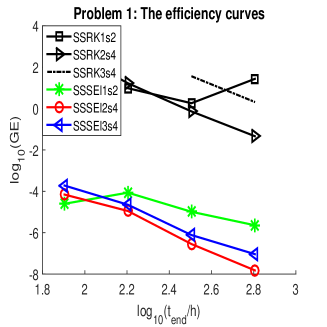
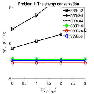
(i)	(ii)

Figure 1: (i): The logarithm of the global error ($GE$) over the integration interval against $t_{end}/h$. (ii): The logarithm of the maximum global error of Hamiltonian $GEH=\max|H_{n}-H_{0}|$ against $\log_{10}(t_{\mathrm{end}})$.

Problem 2. The second numerical example is the following averaged system in wind-induced oscillation

$$\left(\begin{array}[]{c}x_{1}\\ x_{2}\\ \end{array}\right)^{\prime}=\left(\begin{array}[]{cc}-\zeta&-\lambda\\ \lambda&-\zeta\\ \end{array}\right)\left(\begin{array}[]{c}x_{1}\\ x_{2}\\ \end{array}\right)+\left(\begin{array}[]{c}x_{1}x_{2}\\ \frac{1}{2}(x_{1}^{2}-x_{2}^{2})\end{array}\right),$$

where $\lambda=r\sin(\theta)$ is a detuning parameter and $\zeta=r\cos(\theta)\geq 0$ is a damping factor with $r\geq 0,\ 0\leq\theta\leq\pi/2.$ The first integral (when $\theta=\pi/2$) or Lyapunov function (when $\theta<\pi/2$) of this system is

$$H=\frac{1}{2}r(x_{1}^{2}+x_{2}^{2})-\frac{1}{2}\sin(\theta)\big{(}x_{1}x_{2}^{2}-\frac{1}{3}x_{1}^{3}\big{)}+\frac{1}{2}\cos(\theta)\big{(}-x_{1}^{2}x_{2}+\frac{1}{3}x_{2}^{3}\big{)}.$$

We choose the initial values $x_{1}(0)=0,\ x_{2}(0)=1.$ Firstly we consider $\theta=\pi/2,\ r=20$ and solve the problem on the interval $[0,10]$ with $h=\frac{1}{2^{i}}$ for $i=3,4,5,6$. The efficiency curves are shown in Figure 2 (i). Then this problem is integrated with $h=\dfrac{1}{20}$ on the interval $[0,10^{i}],\ i=0,1,2,3.$ See Figure 2 (ii) for the energy conservation for different methods. Secondly we choose $\theta=\pi/2-10^{-4}$ and the efficiency curves are shown in Figure 2 (iii) on $[0,10]$ with $h=\frac{1}{2^{i}},\ i=3,4,5,6.$

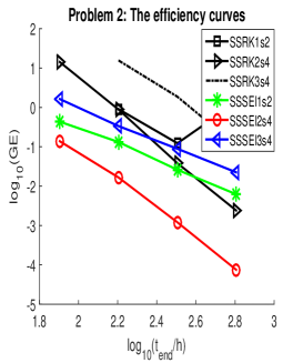
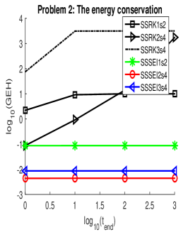
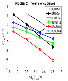
(i)	(ii)	(iii)

Figure 2: (i): The logarithm of the global error ($GE$) over the integration interval against $t_{end}/h$. (ii): The logarithm of the maximum global error of Hamiltonian $GEH=\max|H_{n}-H_{0}|$ against $\log_{10}(t_{\mathrm{end}})$. (iii): The logarithm of the global error ($GE$) over the integration interval against $t_{end}/h$.

From the numerical results, it follows clearly that the symmetric and symplectic exponential integrators behave much better than symmetric and symplectic RK methods.

5 Conclusions and discussions

In this letter, in order to solve the differential equations (1) by using symmetric and symplectic methods, we present the symmetry and symplecticity conditions for exponential integrators. Then based on these conditions, we consider a special kind of exponential integrators and construct some practical symmetric and symplectic exponential integrators. The remarkable efficiency of the new integrators is shown by the numerical results from two numerical experiments in comparison with some existing RK methods in the literature.

References

• [1] H. Berland, B. Owren, B. Skaflestad, B-series and order conditions for exponential integrators, SIAM J. Numer. Anal. 43 (2005) 1715-1727.
• [2] M. Caliari, A. Ostermann, Implementation of exponential Rosenbrock-type integrators, Appl. Numer. Math. 59 (2009) 568-581.
• [3] M.P. Calvo, C. Palencia, A class of explicit multistep exponential integrators for semilinear problems, Numer. Math. 102 (2006) 367-381.
• [4] E. Celledoni, D. Cohen, B. Owren, Symmetric exponential integrators with an application to the cubic Schrödinger equation, Found. Comput. Math. 8 (2008) 303-317.
• [5] V. Grimm, M. Hochbruck, Error analysis of exponential integrators for oscillatory second-order differential equations, J. Phys. A: Math. Gen. 39 (2006) 5495-5507.
• [6] E. Hairer, C. Lubich, G. Wanner, Geometric Numerical Integration: Structure-Preserving Algorithms for Ordinary Differential Equations, 2nd edn. Springer-Verlag, Berlin, Heidelberg, 2006.
• [7] M. Hochbruck, A. Ostermann, Exponential integrators, Acta Numer. 19 (2010) 209-286.
• [8] M. Hochbruck, A. Ostermann, J. Schweitzer, Exponential rosenbrock-type methods, SIAM J. Numer. Anal. 47 (2009) 786-803.
• [9] A. Iserles, On the global error of discretization methods for highly-oscillatory ordinary differential equations, BIT Num. Math. 42 (2002) 561-599.
• [10] A. Iserles, Think globally, act locally: solving highly-oscillatory ordinary differential equations, Appl. Num. Anal. 43 (2002) 145-160.
• [11] A.K. Kassam, L.N.Trefethen, Fourth-order time-stepping for stiff PDEs, SIAM J. Sci. Comput. 26 (2005) 1214-1233.
• [12] M. Khanamiryan, Quadrature methods for highly oscillatory linear and nonlinear systems of ordinary differential equations: part I, BIT Num. Math. 48 (2008) 743-762.
• [13] S. Krogstad, Generalized integrating factor methods for stiff PDEs, J. Comput. Phys. 203 (2005) 72-88.
• [14] L. Mei, X. Wu, Symplectic exponential Runge-Kutta methods for solving nonlinear Hamiltonian systems, J. Comput. Phys. 338 (2017) 567–584.
• [15] A. Ostermann, M. Thalhammer, W.M. Wright, A class of explicit exponential general linear methods, BIT Numer. Math. 46 (2006) 409-431.
• [16] J.M. Sanz-Serna, L. Abia, Order conditions for canonical Runge–Kutta schemes, SIAM J. Numer. Analy. 28 (1991) 1081-1096.
• [17] B. Wang, A. Iserles, X. Wu, Arbitrary–order trigonometric Fourier collocation methods for multi-frequency oscillatory systems, Found. Comput. Math. 16 (2016) 151-181.
• [18] B. Wang, T. Li, Y. Wu, Arbitrary-order functionally fitted energy-diminishing methods for gradient systems, Appl. Math. Lett. 83 (2018) 130-139
• [19] B. Wang, X. Wu, The formulation and analysis of energy-preserving schemes for solving high-dimensional nonlinear Klein-Gordon equations. IMA. J. Numer. Anal. DOI: 10.1093/imanum/dry047 (2018)
• [20] B. Wang, H. Yang, F. Meng, Sixth order symplectic and symmetric explicit ERKN schemes for solving multi-frequency oscillatory nonlinear Hamiltonian equations, Calcolo, 54 (2017) 117-140
• [21] X. Wu, B. Wang, Recent Developments in Structure-Preserving Algorithms for Oscillatory Differential Equations. Springer Nature Singapore Pte Ltd, 2018