Theoretical aspects of quantum electrodynamics
in a finite volume with periodic boundary conditions

Abstract

First-principles studies of strongly-interacting hadronic systems using lattice quantum chromodynamics (QCD) have been complemented in recent years with the inclusion of quantum electrodynamics (QED). The aim is to confront experimental results with more precise theoretical determinations, e.g. for the anomalous magnetic moment of the muon and the CP-violating parameters in the decay of mesons. Quantifying the effects arising from enclosing QED in a finite volume remains a primary target of investigations. To this end, finite-volume corrections to hadron masses in the presence of QED have been carefully studied in recent years. This paper extends such studies to the self-energy of moving charged hadrons, both on and away from their mass shell. In particular, we present analytical results for leading finite-volume corrections to the self-energy of spin-0 and spin-$\frac{1}{2}$ particles in the presence of QED on a periodic hypercubic lattice, once the spatial zero mode of the photon is removed, a framework that is called $\mathrm{QED}_{\mathrm{L}}$. By altering modes beyond the zero mode, an improvement scheme is introduced to eliminate the leading finite-volume corrections to masses, with potential applications to other hadronic quantities. Our analytical results are verified by a dedicated numerical study of a lattice scalar field theory coupled to $\mathrm{QED}_{\mathrm{L}}$. Further, this paper offers new perspectives on the subtleties involved in applying low-energy effective field theories in the presence of $\mathrm{QED}_{\mathrm{L}}$, a theory that is rendered non-local with the exclusion of the spatial zero mode of the photon, clarifying recent discussions on this matter.

I Introduction

State-of-the-art simulations of QCD reliably predict a number of spectral quantities and hadronic matrix elements with a precision below the percent level, see for instance the review by the Flavour Lattice Averaging Group (FLAG) (Aoki et al., 2017). Most of the results listed by FLAG have been obtained within an isospin-symmetric QCD, i.e. , with equal light quark masses and ignoring electromagnetic interactions. A logical next step in the continuous improvement of calculations of spectra, matrix elements and scattering amplitudes is the inclusion of isospin breaking effects, which by naive power counting are expected to contribute at the percent level and are hence becoming significant. First efforts in this direction date back over two decades (Duncan et al., 1996), and interest in this field has picked up considerably over the last few years. First results are now available, in particular, for spectral quantities  (Blum et al., 2007, 2010; Ishikawa et al., 2012; Aoki et al., 2012; Borsanyi et al., 2013, 2015; Portelli, 2015; Horsley et al., 2016a, b; Fodor et al., 2016a; de Divitiis et al., 2013; Giusti et al., 2017a; Basak et al., 2018; Hansen et al., 2018a), and progress is being made in matrix elements and scattering and decay amplitudes (Blum et al., 2017, 2018; Carrasco et al., 2015; Lubicz et al., 2017; Giusti et al., 2018; Christ and Feng, 2018; Giusti et al., 2017b; Boyle et al., 2017).

A fundamental difficulty with the formulation of QED concerns Gauss’ law, which implies that gauge-invariant charged states cannot exist in a finite volume with periodic boundary conditions. As will be discussed later, this problem is related to the occurrence of global photon zero modes. Various proposals exist on how to deal with the zero-mode problem: In $\mathrm{QED}_{\mathrm{TL}}$ (Duncan et al., 1996, 1997; Borsanyi et al., 2013; Ishikawa et al., 2012; Aoki et al., 2012; de Divitiis et al., 2013; Fodor et al., 2016a) the global photon zero mode is removed from the dynamics, while in $\mathrm{QED}_{\mathrm{L}}$ (Hayakawa and Uno, 2008; Davoudi and Savage, 2014; Fodor et al., 2016b; Blum et al., 2007, 2010; Ishikawa et al., 2012; Giusti et al., 2018, 2017a, 2017b; Blum et al., 2018; Boyle et al., 2017; Lee and Tiburzi, 2016; Matzelle and Tiburzi, 2017) the photon zero mode is removed individually on every time slice. Locality is violated in both cases. $\mathrm{QED}_{\mathrm{L}}$ does, however, allow for a transfer matrix to be constructed that is reflection-positive, making it the preferred choice. Understanding and controlling the implications of the locality violation remains an important task. Alternatives to subtracting the zero mode have also been suggested, allowing the locality to be preserved in any finite volume. In massive QED, called $\mathrm{QED}_{\mathrm{M}}$, a small photon mass is introduced as an IR regulator (Endres et al., 2016) and physical QED results are extracted from an extrapolation to the zero photon mass (Endres et al., 2016; Bussone et al., 2018). Charge conjugation boundary conditions (Polley, 1993; Wiese, 1992; Kronfeld and Wiese, 1993, 1991; Lucini et al., 2016; Hansen et al., 2018a) have been proposed as a way to allow the construction of gauge-invariant charged states in a finite volume. In this construction, called $\mathrm{QED}_{\mathrm{C}}$, charge and flavor conservation are partially broken by the boundary conditions and these effects need to be controlled at any finite volume. $\mathrm{QED}_{\mathrm{M}}$ and $\mathrm{QED}_{\mathrm{C}}$ provide promising avenues towards local simulations of QCD+QED.

All approaches introduced above suffer from large finite-volume effects induced by the absence of a mass gap (or the small photon mass in the case of $\mathrm{QED}_{\mathrm{M}}$). Understanding these effects analytically has been the subject of a series of articles (Borsanyi et al., 2015; Davoudi and Savage, 2014; Lubicz et al., 2017; Lucini et al., 2016; Endres et al., 2016). These finite-volume effects are power suppressed in $L$ for massless photons, where $L$ denotes the extent of the finite cubic volume, and their precise form depends on which formulation of QED in a finite volume is implemented. In a number of cases, the leading coefficients of the power expansion are universal. In such cases, the large-distance limit of the finite-volume effects are equivalent to those of point particles and can be computed and corrected for analytically, for instance by means of perturbative calculations in scalar/fermionic QED or in effective field theories, see e.g, Refs. (Borsanyi et al., 2015; Davoudi and Savage, 2014).

The main objective of this paper is to provide a simple and versatile recipe for computing universal finite-volume effects analytically. Some general remarks on $\mathrm{QED}_{\mathrm{TL}}$ and $\mathrm{QED}_{\mathrm{L}}$ are provided, and it is shown how each of these theories are quantized in the path-integral formalism. This is followed by the core part of this paper, namely a proposal for a systematic computation of QED finite-volume effects in terms of a large-volume expansion. Existing results for the finite volume effects on spectral quantities are reproduced and are further extended to on-shell and off-shell finite-volume effects in moving frames, where new rotational symmetry breaking effects are observed and quantified. This recipe is applied to the self-energy of charged fundamental particles with spins 0 and $\frac{1}{2}$. This paper will be followed by another work (Bijnens et al., 2018) by some of the authors, applying the same procedure to compute the finite-volume effects on the electromagnetic corrections to the hadronic vacuum polarization. Inspired by Symanzik’s improvement program aimed at reducing lattice-cutoff effects, a proposal is made for improving the infrared behavior of the $\mathrm{QED}_{\mathrm{L}}$ theory, and is shown to remove universal finite-volume effects by modifying individual momentum modes in the photon action. All the analytical predictions for scalar QED are confirmed by high-statistics simulations. Features of these simulations, such as excited states contributions and the signal-to-noise degradation in boosted systems, are discussed. We conclude this paper with clarifying remarks on effective theories of $\mathrm{QED}_{\mathrm{L}}$. This discussion provides insights into the origin of the discrepancy between full $\mathrm{QED}_{\mathrm{L}}$ and its corresponding effective theories for the higher-order finite-volume QED effects. New local operators with volume-dependent coefficients are introduced into the effective theories without the need to include the anti-particle modes.

II $\mathrm{QED}_{\mathrm{L}}$ in the path integral formalism

In this section we retrace the construction of $\mathrm{QED}_{\mathrm{L}}$, first introduced in Ref. (Hayakawa and Uno, 2008) from the point of view of path integral quantization. While most readers will be familiar with the definition of $\mathrm{QED}_{\mathrm{L}}$, we provide a more formal definition in terms of the path integral as the starting point for perturbative expansions or lattice discretizations discussed in later sections. We start by making general observations about QED in a finite volume and then introduce $\mathrm{QED}_{\mathrm{TL}}$ and $\mathrm{QED}_{\mathrm{L}}$.

II.1 Periodic fields and zero-mode singularities

The infinite-volume Euclidean Maxwell action in Feynman gauge is

$$S[A_{\mu}]= \int\mathrm{d}^{4}x\left\{\frac{1}{4}F_{\mu\nu}(x)F_{\mu\nu}(x)+\frac{1}{2}[\partial_{\mu}A_{\mu}(x)]^{2}\right\}$$

$$= -\frac{1}{2}\int\mathrm{d}^{4}x\,A_{\mu}(x)\,\partial^{2}A_{\mu}(x)\,,$$ (1)

where $F_{\mu\nu}=\partial_{\mu}A_{\nu}-\partial_{\nu}A_{\mu}$ is the field strength tensor and $A_{\mu}$ is the $\operatorname{U}(1)$ gauge potential. In momentum space, this action takes the convenient form

$$S[\hat{A}_{\mu}]=\frac{1}{2}\int\frac{\mathrm{d}^{4}k}{(2\pi)^{4}}\ k^{2}\ {\textstyle\sum_{\mu}}|\hat{A}_{\mu}(k)|^{2}\,,$$ (2)

where the following Fourier transform normalization is used

$$\hat{A}_{\mu}(k)=\int\mathrm{d}^{4}x\,A_{\mu}(x)e^{-ik\cdotp x}\,.$$ (3)

The theory is quantized by means of the Euclidean path integral. The vacuum expectation value of operator $O$ in the absence of matter fields is defined as

$$\braket{O}=\frac{1}{\mathcal{Z}}\int\mathcal{D}A_{\mu}\,O[A_{\mu}]\exp(-S[A_{\mu}])\,,$$ (4)

where $\mathcal{Z}=\int\mathcal{D}A_{\mu}\exp(-S[A_{\mu}])$ is the partition function. In this free theory, any expectation value can be expressed in terms of the photon propagator

$$D_{\mu\nu}^{(\infty)}(x-y)=-\delta_{\mu\nu}(\partial^{2})^{-1}\delta(x-y)=\int\frac{\mathrm{d}^{4}k}{(2\pi)^{4}}\frac{\delta_{\mu\nu}}{k^{2}}e^{ik\cdotp(x-y)}\,.$$ (5)

The inverse Laplacian is defined unambiguously in infinite volume since its zero mode constitutes a set of measure zero within the continuous spectrum of the operator.

Now consider the above path integral in a finite volume of spacetime with spatial dimensions of equal length $L$ and a time extent $T$. Here, periodic boundary conditions are imposed, and the physical space-time volume is denoted by $\mathbb{T}^{4}$. For the sake of simplicity and since we are only interested in long-distance effects, spacetime is assumed to be continuous. Momentum is quantized on $\mathbb{T}^{4}$, and the Fourier transform is defined by

$$\hat{f}(k)=\int_{\mathbb{T}^{4}}\mathrm{d}^{4}x\,f(x)e^{-ik\cdotp x}\qquad\text{and}\qquad f(x)=\frac{1}{TL^{3}}\sum_{k\in\hat{\mathbb{T}}^{4}}\hat{f}(k)e^{ik\cdotp x}\,,$$ (6)

where $\hat{\mathbb{T}}^{4}$ is the discrete set of vectors of the form $(\frac{2\pi}{T}n_{0},\frac{2\pi}{L}\mathbf{n})$ where $n=(n_{0},\mathbf{n})$ is a four-vector with integer components. On $\mathbb{T}^{4}$, one could attempt to define QED in terms of the continuum limit of a discretized version of the momentum-space action given in eq. 2:

$$S[\hat{A}_{\mu}]=\frac{1}{2TL^{3}}\sum_{k\in\hat{\mathbb{T}}^{4}}k^{2}\,{\textstyle\sum_{\mu}}|\hat{A}_{\mu}(k)|^{2}\,.$$ (7)

In this case, the zero mode of the Laplacian is a significant, isolated mode, and the finite-volume equivalent of eq. 5,

$$D_{\mu\nu}(x-y)=\frac{1}{TL^{3}}\sum_{k\in\hat{\mathbb{T}}^{4}}\frac{\delta_{\mu\nu}}{k^{2}}e^{ik\cdotp(x-y)}\,,$$ (8)

is ill-defined because of the singular $k=0$ term in the sum. In other words, the Laplacian is not invertible. Now let us define a shift transformation through

$$A_{\mu}(x)\mapsto A_{\mu}^{b}(x)=A_{\mu}(x)+\frac{b_{\mu}}{TL^{3}}\,,$$ (9)

where $b_{\mu}$ is a constant four-vector with a mass dimension equal to $-3$. In momentum space, this shift transformation becomes

$$\hat{A}_{\mu}^{b}(k)=\hat{A}_{\mu}(k)+b_{\mu}\delta_{k,0}\,,$$ (10)

i.e. it modifies the zero-mode of the EM potential. The action in  eq. 7 is invariant under such shift transformations and hence the Laplacian is not invertible. One can in fact show that for periodic boundary conditions shift transformations span the whole nullspace of the Laplacian.

One can observe that in eq. 9, the shift $b_{\mu}$ can in principle be written as the derivative of a linear function $\omega$, which makes the shift transformation a gauge transformation. To be smooth, the associated $\operatorname{U}(1)$ transformation $\exp(i\omega)$ requires $b_{\mu}$ to fullfil some trivial quantization condition. Such function is not homotopic to the identity on $\operatorname{U}(1)$, and is part of the class of “large” gauge transformations. As it will be discussed at length in the next sections, the redundancy associated to these transformations cannot be fixed using a local gauge fixing prescription.

II.2 The $\mathrm{QED}_{\mathrm{TL}}$ theory

The shift symmetry described in the previous section is somewhat similar to the problem in gauge theory that motivates gauge fixing: the action of the theory has an internal symmetry which generates a singular redundancy in the space of field configurations. In the case of shift symmetry, this redundancy can be eliminated by using the same Fadeev and Popov procedure (Faddeev and Popov, 1967) that is used to implement gauge fixing in the path integral formalism of gauge theories. We start by inserting

$$1=\int\mathrm{d}b_{\mu}\ \delta[{\textstyle\int_{\mathbb{T}^{4}}}\mathrm{d}^{4}x\,A_{\mu}^{b}(x)]\,,$$ (11)

into the path integral in eq. 4,

$$\braket{O}=\frac{1}{\mathcal{Z}}\int\mathcal{D}A_{\mu}\int\mathrm{d}b_{\mu}\,\delta\left[{\textstyle\int_{\mathbb{T}^{4}}}\mathrm{d}^{4}x\,A_{\mu}^{b}(x)\right]O[A_{\mu}]\exp(-S[A_{\mu}])\,.$$ (12)

Using the invariance of the action under $A_{\mu}\mapsto A_{\mu}^{b}$ and assuming the same property for the operator, the infinite factor of $\int\mathrm{d}b_{\mu}$ can be canceled between the numerator and the denominator to obtain

$$\braket{O}=\frac{1}{\mathcal{Z}_{\mathrm{TL}}}\int\mathcal{D}A_{\mu}\,\delta\left[{\textstyle\int_{\mathbb{T}^{4}}}\mathrm{d}^{4}x\,A_{\mu}(x)\right]O[A_{\mu}]\exp(-S[A_{\mu}])\,,$$ (13)

which corresponds to restricting the integrations to the subspace of field configurations with a vanishing zero mode. Reusing the nomenclature from Ref. (Borsanyi et al., 2015), we reference the theory associated with  eq. 13 as $\mathrm{QED}_{\mathrm{TL}}$. With the removal of the zero-mode redundancy, the $\mathrm{QED}_{\mathrm{TL}}$ photon two-point function is well defined:

$$D_{\mu\nu}^{(\mathrm{TL})}(x-y)=\frac{1}{TL^{3}}\operatorname*{\sideset{}{{}^{\prime}}{\sum}}_{k\in\hat{\mathbb{T}}^{4}}\frac{\delta_{\mu\nu}}{k^{2}}e^{ik\cdotp(x-y)}\,,$$ (14)

where the primed sum indicates that the $k=0$ term is excluded from the summation.

At first sight, $\mathrm{QED}_{\mathrm{TL}}$ appears to be an acceptable solution to the zero-mode problem, and it has in fact been used in numerous lattice QED calculations (Duncan et al., 1996; Borsanyi et al., 2013; de Divitiis et al., 2013; Borsanyi et al., 2015). However, as first noticed in Ref. (Borsanyi et al., 2015), problems arise when one tries to couple $\mathrm{QED}_{\mathrm{TL}}$ to matter fields. The source term

$$S_{\text{int.}}[A_{\mu},J_{\mu}]=\int_{\mathbb{T}^{4}}\mathrm{d}^{4}x\,A_{\mu}(x)J_{\mu}(x)\,,$$ (15)

which couples photons $(A_{\mu})$ to an external current $J_{\mu}$, is not invariant under shift transformations and matter therefore couples to unphysical photon zero modes. A way out of this problem is provided by the shift-invariant interaction term

$$S_{\mathrm{TL},\text{int.}}[A_{\mu},J_{\mu}]=\int_{\mathbb{T}^{4}}\mathrm{d}^{4}x\,A_{\mu}(x)\left[J_{\mu}(x)-{\textstyle\frac{1}{TL^{3}}\int_{\mathbb{T}^{4}}\mathrm{d}^{4}y\,J_{\mu}(y)}\right]\,.$$ (16)

However, dealing with the photon zero mode in this way introduces a non-locality in space and time: the field $A_{\mu}$ at a point $x$ couples to $J_{\mu}$ at all points in spacetime. This seems to be unavoidable if one wants to completely decouple the zero mode from the theory. In $\mathrm{QED}_{\mathrm{TL}}$, this has severe consequences: if for instance $J_{\mu}$ is not a classical background current but the fermionic vector current $\overline{\psi}\gamma_{\mu}\psi$, the non-locality in time renders the definition of a bounded transfer matrix for the matter fields impossible. As a consequence, this theory cannot be continued to a quantum field theory in Minkowski spacetime and it has a divergent $T\to+\infty$ limit. This divergence has been shown explicitly for masses of spin $0$ and $\frac{1}{2}$ particles calculated in $\mathrm{QED}_{\mathrm{TL}}$ in Ref. (Borsanyi et al., 2015). This problem could be circumvented by taking the $L\to+\infty$ limit first, ending up in a theory equivalent to QED at finite temperature which has the correct $T\to+\infty$ (zero-temperature) limit.

II.3 The $\mathrm{QED}_{\mathrm{L}}$ theory

An alternative way of dealing with the zero mode which maintains locality of the interaction term in time is provided by

$$S_{\mathrm{L},\text{int.}}[A_{\mu},J_{\mu}]=\int_{\mathbb{T}^{4}}\mathrm{d}^{4}x\,A_{\mu}(x)\left[J_{\mu}(x)-{\textstyle\frac{1}{L^{3}}\int_{\mathbb{T}^{3}}\mathrm{d}^{3}\mathbf{y}\,J_{\mu}(t,\mathbf{y})}\right]\,,$$ (17)

where $x=(t,\mathbf{x})$ and $\mathbb{T}^{3}$ is the 3-dimensional periodic space of extent $L$. This term is shift invariant under the symmetry group

$$A_{\mu}(x)\mapsto A_{\mu}(x)+\frac{b_{\mu}(t)}{L^{3}}\,,$$ (18)

where $b_{\mu}(t)$ is an arbitrary smooth four-vector function of the time coordinate with mass dimension $-2$. The modification to the current in eq. 17 can be interpreted as placing a uniform charge (current) density in the volume, whose effect is to restore Gauss’ (Ampere’s) law in a finite volume with periodic boundary conditions (Hayakawa and Uno, 2008). As a result, matter is decoupled from all field configurations which are constant in space. In an infinite volume, fields are however assumed to vanish at infinity and so these configurations seem unphysical yet again. Following a procedure similar to the one laid out in the previous section, all spatial zero modes can be removed by introducing the shift symmetry fixing term $\delta[\int_{\mathbb{T}^{3}}\mathrm{d}^{3}\mathbf{x}\,A_{\mu}(t,\mathbf{x})]$. As we know from the previous discussions of $\mathrm{QED}_{\mathrm{TL}}$, the photon action is invariant under the shift transformation in eq. 18 only through the presence of constant modes. Removing these modes leads to the path integral

$$\braket{O}=\frac{1}{\mathcal{Z}_{\mathrm{L}}}\int\mathcal{D}A_{\mu}\,\delta\left[{\textstyle\int_{\mathbb{T}^{3}}}\mathrm{d}^{3}\mathbf{x}\,A_{\mu}(t,\mathbf{x})\right]O[A_{\mu}]\exp(-S[A_{\mu}]-S_{\mathrm{L},\text{int.}}[A_{\mu},J_{\mu}])\,.$$ (19)

This integral defines $\mathrm{QED}_{\mathrm{L}}$. It was first proposed in Ref. (Hayakawa and Uno, 2008), and the differences between $\mathrm{QED}_{\mathrm{L}}$ and $\mathrm{QED}_{\mathrm{TL}}$ were later discussed in Ref. (Borsanyi et al., 2015). It can be shown that the $\mathrm{QED}_{\mathrm{L}}$ action fulfills the requirement of reflection positivity, which therefore guarantees the existence of a well-defined transfer matrix and can be analytically continued to a Minkowski quantum field theory. As a consequence, when a mass gap exists, as in the case of hadronic states in QCD, observables asymptote to their value at $T\to+\infty$ exponentially fast. As $\mathrm{QED}_{\mathrm{L}}$ will be considered in the rest of this paper, the temporal extent is assumed to be infinite in all discussions that will follow.

Although $\mathrm{QED}_{\mathrm{L}}$ solves problems associated with defining a transfer matrix, it remains non-local in space. Naively, this non-locality is merely a finite-volume effect and all correlation functions computed in $\mathrm{QED}_{\mathrm{L}}$ are expected to converge to those of QED in the infinite-volume limit. This is certainly true classically: the non-local term in eq. 17 vanishes in the infinite-volume limit. One might worry, however, that short-distance divergences could in principle couple to volume effects through radiative corrections, making the renormalization of $\mathrm{QED}_{\mathrm{L}}$ ambiguous. In fact, hints of subtleties arising from an incomplete decoupling of short-distance and long-distance effects are seen in attempting to describe the interactions of massive matter fields with photons in $\mathrm{QED}_{\mathrm{L}}$ using a heavy-field effective theory approach, as discussed in section VI. Nonetheless, quantities that have been studied to date with lattice QCD+QED calculations appear not to suffer from this problem. Whether this will become an issue in future higher-precision calculations, or in calculations of other quantities, remains to be determined.

At the core of the issues discussed here are the periodic boundary conditions which allow for constant field configurations to be present. Authors of Ref. (Lucini et al., 2016) proposed to use boundary conditions for which all particles undergo a charge conjugation transformation at every period. In that formulation, the photon field is antiperiodic and therefore does not have a zero mode, allowing for the definition of a local theory in a finite volume. However, this theory exhibits a few non-trivial features, such as the non-conservation of electric charge and flavor quantum numbers. Realistic numerical simulations implementing this construction are underway (Hansen et al., 2018b; Campos, Isabel and Fritzsch, Patrick and Hansen, Martin and Marinković, Marina Krstić and Patella, Agostino and Ramos, Alberto and Tantalo, Nazario, 2018; Hansen et al., 2018a) and can establish if there are advantages to be gained with this formulation of QED in finite volume compared with others, such as those introduced in this section, or one in which the zero mode of the photon is avoided by introducing a small photon mass (Endres et al., 2016). In $\mathrm{QED}_{\mathrm{M}}$, the photon is endowed with a small mass, $m_{\gamma}$, that localizes the range of the electromagnetic interactions between charged particles to volumes within a radius of $\sim 1/m_{\gamma}$, screening electric charges. This construction explicitly violates Gauss’s Law without the removal of modes of the electromagnetic field by including a mass gap into the theory. Consequently, in volumes of spatial extent $L$, modifications to localized observables, such as the mass of a charged particle, are exponentially insensitive to the finite volume for $m_{\gamma}L\sim 4$. However, the observables depend explicitly upon $m_{\gamma}$. To recover infinite-volume values of observables, an extrapolation to $m_{\gamma}=0$ is required. Using (local) EFTs to cleanly separate UV and IR physics scales, the counterterms defining the EFT are polynomial functions of $m_{\gamma}$, which can be determined by fitting to results of lattice calculations performed in a range of volumes that satisfy $m_{\gamma}L\sim 4$. The $m_{\gamma}=0$ values can then be identified. The EFT can be used, with these $m_{\gamma}=0$ counterterms, to make predictions. For this technique to provide a complete quantification of uncertainties, a hierarchy of scales between $m_{\gamma}$ and the lightest hadron mass $m_{H}$, $m_{\gamma}/m_{H}\ll 1$, must exists to ensure that the counterterms only involve polynomials in $m_{\gamma}$. This in turn requires large-volume lattice simulations, with volumes of QCD+$\mathrm{QED}_{\mathrm{M}}$ calculations that are significantly larger than for QCD calculations.

III Finite-size effects in $\mathrm{QED}_{\mathrm{L}}$: the self-energy function

In this section, we compute the volume dependence of the $\mathrm{QED}_{\mathrm{L}}$ self-energy functions for spins $0$ and $\frac{1}{2}$ fundamental charged particles. Such corrections are obtained for the first time in the present paper for moving particles in a finite cubic volume with periodic boundary conditions, both on and away from their mass shell.

III.1 Finite-volume effects in the self-energy function

III.1.1 Formal definition

We consider $\mathrm{QED}_{\mathrm{L}}$, as described in the previous section, coupled to QCD interaction through the usual gauge-covariant coupling of the Dirac quark action to $\mathrm{QED}_{\mathrm{L}}$ and the $\operatorname{SU}(3)$ Yang-Mills gauge action representing the gluon fields. In this context, we are interested in the propagation amplitude of a given hadronic state $\ket{X}$, which can be interpolated through the 2-point function of a given operator $\phi_{X}$ with the same conserved quantum numbers as the physical state $\ket{X}$. Expanding in the electromagnetic coupling constant, we obtain the second-order electromagnetic corrections to this 2-point function as $D_{\mu\nu}(y_{1}-y_{2})\,C_{\mu\nu}(x_{1},y_{1},x_{2},y_{2})$, where

$$C_{\mu\nu}(x_{1},y_{1},x_{2},y_{2})=\bra{0}\mathrm{T}[\phi_{X}(x_{1})J_{\mu}(y_{1})J_{\nu}(y_{2})\phi_{X}(x_{2})^{\dagger}]\ket{0}\,,$$ (20)

and where $J_{\mu}$ is the electromagnetic current. The associated momentum-space correlation function $G_{\mu\nu}(p_{1},k_{1},k_{2})$ can be defined through

$$G_{\mu\nu}(p_{1},k_{1},k_{2})=\int\mathrm{d}^{4}x_{1}\int\mathrm{d}^{4}y_{1}\int\mathrm{d}^{4}y_{2}\,C_{\mu\nu}(x_{1},y_{1},0,y_{2})e^{i(-p_{1}\cdotp x_{1}-k_{1}\cdotp y_{1}+k_{2}\cdotp y_{2})}\,.$$ (21)

This function can be amputated to define the corresponding vertex function

$$\Gamma_{\mu\nu}(p_{1},k_{1},k_{2})=G(p_{1})^{-1}G_{\mu\nu}(p_{1},k_{1},k_{2})G(p_{1}+k_{1}-k_{2})^{-1}\,,$$ (22)

where $G(p)$ is the momentum-space 2-point function of field $\phi_{X}$,

$$G(p)=\int\mathrm{d}^{4}x\bra{0}\mathrm{T}[\phi_{X}(x)\phi_{X}(0)^{\dagger}]\ket{0}e^{-ip\cdotp x}\,.$$ (23)

From these definitions, the self-energy function of $X$ is given by

$$\Sigma(p)=\int\frac{\mathrm{d}^{4}k}{(2\pi)^{4}}K(k,p)\,,$$ (24)

where $K(k,p)$ is the electromagnetic kernel,

$$K(k,p)=D_{\mu\nu}(k)\Gamma_{\mu\nu}(p,k,k)\,,$$ (25)

with $D_{\mu\nu}(k)$ the free photon propagator in a given gauge. In Euclidean spacetime, the on-shell self-energy can be obtained by setting $p=(i\omega(\mathbf{p}),\mathbf{p})$ with $\omega(\mathbf{p})=\sqrt{\mathbf{p}^{2}+m^{2}}$.

Now consider a hypercubic spacetime that has infinite extent in the time direction, and is periodic in spatial directions with a finite extent $L$. In this construction, the $\mathrm{QED}_{\mathrm{L}}$ self-energy is given by

$$\Sigma^{(L)}(p)=\frac{1}{L^{3}}\operatorname*{\sideset{}{{}^{\prime}}{\sum}}_{\mathbf{k}\in\hat{\mathbb{T}}^{3}}\int\frac{\mathrm{d}k_{0}}{2\pi}K(k,p)\,,$$ (26)

where, as defined in section II, $\hat{\mathbb{T}}^{3}$ is the set of three-vectors of the form $\frac{2\pi}{L}\mathbf{n}$ where $\mathbf{n}$ has integer components. The $\mathrm{QED}_{\mathrm{L}}$ finite-volume effects in the self-energy are then given by

$$\Delta\Sigma(p)=\Sigma(p)-\Sigma^{(L)}(p)=\left(\frac{1}{L^{3}}\operatorname*{\sideset{}{{}^{\prime}}{\sum}}_{\mathbf{k}\in\hat{\mathbb{T}}^{3}}-\int\frac{\mathrm{d}^{3}\mathbf{k}}{(2\pi)^{3}}\right)\int\frac{\mathrm{d}k_{0}}{2\pi}\,K(k,p)\,.$$ (27)

By rescaling the loop 3-momentum by $\frac{2\pi}{L}$, this expression can be written in the compact form

$$\Delta\Sigma(p)=\frac{1}{L^{3}}\Delta_{\mathbf{n}}^{\prime}\int\frac{\mathrm{d}k_{0}}{2\pi}\,K((k_{0},{\textstyle\frac{2\pi}{L}}\mathbf{n}),p)\,,$$ (28)

where $\Delta_{\mathbf{n}}^{\prime}$ is defined as the the sum-integral difference

$$\Delta_{\mathbf{n}}^{\prime}=\operatorname*{\sideset{}{{}^{\prime}}{\sum}}_{\mathbf{n}\in\mathbb{Z}^{3}}-\int\mathrm{d}^{3}\mathbf{n}\,.$$ (29)

Because of the singularities in the kernel $K(k,p)$ at zero photon momentum, $\Delta\Sigma(p)$ is expected to behave like a polynomial in $\frac{1}{L}$ at large $L$. Moreover, it has been shown (Borsanyi et al., 2015; Lubicz et al., 2017) using a generic low-energy effective representation of $\Gamma_{\mu\nu}$ that the two first orders of this expansion are universal, i.e. they do not depend on the structure of the hadron $X$ and can be obtained in the point-like approximation. This important fact is shown to be a direct consequence of gauge invariance, which constrains the form of $\Gamma_{\mu\nu}$ through Ward-Takahashi identities.

The main purpose of the present work is to discuss how to generalize electromagnetic finite-volume calculations to virtual processes and moving frames, and discuss the qualitative properties of the results. Therefore, we will only consider the case of point-like particles, although all the aspects discussed below generalize to the case of composite particles, given an appropriate parametrization of the vertex function $\Gamma_{\mu\nu}$.

III.1.2 Point-like spin $0$ and $\frac{1}{2}$ electromagnetic self-energy functions

In finite (infinite) Euclidean spacetime and at $\mathcal{O}(q^{2})$, the self-energy of massive point-like particles with electric charge $q$, mass $m$, and four-momentum $p=(p_{0},\mathbf{p})$ are given by sums (integrals) over the photon momentum $k=(k_{0},\mathbf{k})$ of the kernels

$$K_{0}(k,p) =q^{2}\left\{\frac{4}{k^{2}}-\frac{(2p-k)^{2}}{k^{2}[(p-k)^{2}+m^{2}]}\right\},$$ (30)

$$K_{\frac{1}{2}}(k,p) =q^{2}\left\{\frac{2i(\not{p}-\not{k})+4m}{k^{2}[(p-k)^{2}+m^{2}]}\right\}\,,$$ (31)

for spins $0$ and $\frac{1}{2}$, respectively (see fig. 1). In what follows, strategies to obtain the large-volume expansion of the finite-volume effects associated with these kernels are discussed.

Figure 1: The self-energy of a scalar point-like particle at $\mathcal{O}(\alpha)$ consists of diagrams shown with one-photon and two-photon couplings $-q(p_{1}+p_{2})^{\mu}$ and $-2q^{2}\delta_{\mu\nu}$, respectively, where $p_{1}(p_{2})$ is the incoming (outgoing) particle momentum. The self-energy of a point-like spin-$\frac{1}{2}$ particle at $\mathcal{O}(\alpha)$ is given by the diagram in the left panel with the one-photon coupling $-q\gamma_{\mu}$, where $\gamma_{\mu}$ is an Euclidean Dirac gamma matrix.

III.2 Large-volume expansion

III.2.1 General result

It is natural to use the on-shell energy $\omega(\mathbf{p})=\sqrt{\mathbf{p}^{2}+m^{2}}$ as a reference scale, in terms of which the infinite-volume limit is taken as $L\,\omega(\mathbf{p})\to+\infty$. Useful dimensionless ratios with $\omega(\mathbf{p})$ are the $\sigma$-ratio

$$\sigma=\frac{p^{2}+m^{2}}{\omega(\mathbf{p})^{2}}=\frac{p_{0}^{2}}{\omega(\mathbf{p})^{2}}+1\,,$$ (32)

and the velocity

$$\mathbf{v}=\frac{\mathbf{p}}{\omega(\mathbf{p})}\,.$$ (33)

The $\sigma$-ratio is positive and vanishes for an on-shell external state (i.e. $p^{2}=-m^{2}$). More precisely, in Euclidean spacetime $\sigma\geq 1$ and correlation functions can be analytically continued to $0\leq\sigma<1$, where $\sigma=0$ is the on-shell point. The velocity has a magnitude strictly smaller than one for massive particles. In terms of these parameters, the external momentum can be expressed as

$$p=\omega(\mathbf{p})(\sqrt{\sigma-1},\mathbf{v})\,,$$ (34)

hence any function of $p$ can be expressed as a function of $\omega(\mathbf{p})$, $\sigma$ and $\mathbf{v}$.

The calculation of the finite-volume effects proceeds as follows. Consider a kernel of the form

$$K(k,p)=\frac{f(k,p)}{k^{2}[(p-k)^{2}+m^{2}]}\,,$$ (35)

where the numerator $f(k,p)$ is an analytic function in $k$ and $p$. Performing the $k_{0}$ integration, we obtain

$$\int\frac{\mathrm{d}k_{0}}{2\pi}\,K(k,p)=R_{\gamma}(\mathbf{k},p)+R_{m}(\mathbf{k},p)\,,$$ (36)

with the upper-plane residues

$$R_{\gamma}(\mathbf{k},p)=i\operatorname{Res}_{k_{0}=i|\mathbf{k}|}K(k,p)\qquad\text{and}\qquad R_{m}(\mathbf{k},p)=i\operatorname{Res}_{k_{0}=p_{0}+i\omega(\mathbf{p}-\mathbf{k})}K(k,p)\,.$$ (37)

Now using eq. 28, the finite-volume effects in the self-energy are given by

$$\Delta\Sigma(p)=\Delta_{\gamma}(p)+\Delta_{m}(p)\,,$$ (38)

with

$$\Delta_{j}(p)=\frac{1}{L^{3}}\Delta_{\mathbf{n}}^{\prime}R_{j}({\textstyle\frac{2\pi}{L}\mathbf{n}},p)\,,$$ (39)

for $j=\gamma,m$. These effects can be directly computed by studying the behavior of the residues around $\mathbf{k}=\mathbf{0}$. In this section, only the explicit results are presented and further details of the derivations can be found in appendix A.

For the on-shell momentum $p=p_{\mathrm{o.s.}}=(i\omega(\mathbf{p}),\mathbf{p})$, the photon-pole finite-volume effect is given by

$$\Delta_{\gamma}(p_{\mathrm{o.s.}})=\frac{f_{0}(p_{\mathrm{o.s.}})c_{2,1}(\mathbf{v})}{16\pi^{2}\omega(\mathbf{p})L}+\sum_{j=1}^{+\infty}\frac{\xi_{2-j,1,j}(p_{\mathrm{o.s.}})}{2^{4-j}\pi^{2-j}\omega(\mathbf{p})L^{1+j}}+\cdots\,,$$ (40)

where the ellipsis denote exponentially suppressed finite-volume effects, and the coefficients $f_{j}(\hat{\mathbf{k}},p)$, $c_{j,k}(\mathbf{v})$, and $\xi_{j,k}(\mathbf{p})$ are defined by

$$f((i|\mathbf{k}|,\mathbf{k}),p) =f_{0}(p)+\sum_{j=1}^{+\infty}f_{j}(\hat{\mathbf{k}},p)|\mathbf{k}|^{j}\,,$$ (41)

$$c_{j,k}(\mathbf{v}) =\Delta_{\mathbf{n}}^{\prime}\left[\frac{1}{|\mathbf{n}|^{j}(1-\mathbf{v}\cdot\hat{\mathbf{n}})^{k}}\right]\,,$$ (42)

$$\xi_{j,k,l}(p) =\Delta_{\mathbf{n}}^{\prime}\left[\frac{f_{l}(\hat{\mathbf{n}},p)}{|\mathbf{n}|^{j}(1-\mathbf{v}\cdot\hat{\mathbf{n}})^{k}}\right]\,.$$ (43)

The coefficient $c_{j,k}(\mathbf{v})$ that drives the leading-order correction is particularly important as it appears systematically in perturbative calculations of QED finite-size effects. The properties and evaluation of these numbers are studied in detail in section III.3. We also define the rest-frame coefficients

$$c_{j}=c_{j,k}(\mathbf{0})=\Delta_{\mathbf{n}}^{\prime}\frac{1}{|\mathbf{n}|^{j}}\,.$$ (44)

These coefficients can be seen as particular values of the generalized zeta function from Ref. (Luscher, 1986), i.e. $c_{j}=Z_{00}(\frac{j}{2},\mathbf{0})$, and have the known values

$$c_{2}=\pi c_{1},\qquad c_{1}=-2.83729748\dots,\qquad\text{and}\qquad c_{0}=-1\,.$$ (45)

In the off-shell case, one obtains

$$\Delta_{\gamma}(p)=\frac{f_{0}(p)c_{1}}{4\pi\sigma\omega(\mathbf{p})^{2}L^{2}}+\left[-\frac{i\sqrt{\sigma-1}\,f_{0}(p)}{\sigma^{2}\omega(\mathbf{p})^{3}}+\frac{\xi_{0,0,1}(p)}{2\sigma\omega(\mathbf{p})^{2}}\right]\frac{1}{L^{3}}+\operatorname{\mathcal{O}}\left(\frac{1}{L^{4}}\right)\,.$$ (46)

We observe that in this case the absence of the on-shell singularity pushes the finite-volume effects to $\operatorname{\mathcal{O}}(\frac{1}{L^{2}})$. The charged-particle effect $\Delta_{m}(p)$ is $\operatorname{\mathcal{O}}(\frac{1}{L^{3}})$ independently of on-shell conditions and it is given by

$$\Delta_{m}(p)=-\frac{r_{m}(\mathbf{0},p)}{L^{3}}+\cdots=-\frac{f(((i+\sqrt{\sigma-1})\omega(\mathbf{p}),\mathbf{0}),p)}{2(i+\sqrt{\sigma-1})^{2}\omega(\mathbf{p})^{3}L^{3}}+\cdots\,.$$ (47)

III.2.2 Spin-$0$ self-energy

The strategy described in the previous section can be applied to the kernel in eq. 30. In this case, the function $f$ is given by

$$f(k,p)=q^{2}(3k^{2}-4p\cdot k+4m^{2})\,,$$ (48)

and the coefficients $f_{j}$ defined in eq. 41 are

$$f_{0}(p)=4q^{2}m^{2},\qquad f_{1}(\hat{\mathbf{k}},p)=-4q^{2}[ip_{0}+\omega(\mathbf{p})(\mathbf{v}\cdot\hat{\mathbf{k}})]\,,$$ (49)

and $f_{j}=0$ for $j>1$. Considering eqs. 40 and 46, the only required $\xi_{j,k,l}(p)$ coefficients are

$$\xi_{1,1,1}(p)=4q^{2}\omega(\mathbf{p})c_{1}\qquad\text{and}\qquad\xi_{0,0,1}(p)=-4iq^{2}p_{0}c_{0}=4iq^{2}p_{0}\,.$$ (50)

Substituting relevant functions in eq. 40, the on-shell finite-volume effects from the photon pole are given by

$$\Delta_{\gamma}(p_{\mathrm{o.s.}}) =q^{2}\left[\frac{m^{2}c_{2,1}(\mathbf{v})}{4\pi^{2}\omega(\mathbf{p})L}+\frac{c_{1}}{2\pi L^{2}}+\cdots\right]$$ (51)

$$=m^{2}q^{2}\left[\frac{1}{\gamma(|\mathbf{v}|)}\frac{c_{2,1}(\mathbf{v})}{4\pi^{2}\mu}+\frac{c_{1}}{2\pi\mu^{2}}+\cdots\right]\,,$$ (52)

where $\mu=mL$, and $\gamma(|\mathbf{v}|)=(1-|\mathbf{v}|^{2})^{-1/2}$ is the usual Lorentz contraction factor. For the scalar-particle pole, the effects are

$$\Delta_{m}(p_{\mathrm{o.s.}})=m^{2}q^{2}\left[\frac{1}{\gamma(|\mathbf{v}|)^{3}}-\frac{1}{\gamma(|\mathbf{v}|)}\right]\frac{1}{2\mu^{3}}+\cdots\,.$$ (53)

on shell. Putting everything together, the finite-volume effects on the self energy of a moving on-shell spin-$0$ particle are

$$\Delta\omega_{0}(\mathbf{p})^{2}=\Delta\Sigma(p_{\mathrm{o.s.}})=m^{2}q^{2}\left\{\frac{1}{\gamma(|\mathbf{v}|)}\frac{c_{2,1}(\mathbf{v})}{4\pi^{2}\mu}+\frac{c_{1}}{2\pi\mu^{2}}+\left[\frac{1}{\gamma(|\mathbf{v}|)^{3}}-\frac{1}{\gamma(|\mathbf{v}|)}\right]\frac{1}{2\mu^{3}}+\cdots\right\}\,,$$ (54)

In the off-shell case, using eqs. 40 and 47, the photon-pole and particle-pole effects are

$$\Delta_{\gamma}(p)=m^{2}q^{2}\left\{\frac{1}{\gamma(|\mathbf{v}|)^{2}}\frac{c_{1}}{\pi\sigma\mu^{2}}+\left[\frac{2i\sqrt{\sigma-1}}{\gamma(|\mathbf{v}|)\sigma}-\frac{4i\sqrt{\sigma-1}}{\gamma(|\mathbf{v}|)^{3}\sigma^{2}}\right]\frac{1}{\mu^{3}}+\operatorname{\mathcal{O}}\left(\frac{1}{\mu^{4}}\right)\right\}\,,$$ (55)

and

$$\Delta_{m}(p)=m^{2}q^{2}\left[\frac{\sigma-4-4i\sqrt{\sigma-1}}{2\sigma\gamma(|\mathbf{v}|)}-\frac{2}{(i+\sqrt{\sigma-1})^{2}\gamma(|\mathbf{v}|)^{3}}\right]\frac{1}{\mu^{3}}+\cdots,$$ (56)

respectively. Note that this pole contribution has no on-shell singularities, and the on-shell effects are obtained by taking the limit $\sigma\to 0$, consistent with eq. 53. Finally, the finite-volume effect in the off-shell self-energy of a moving spin-0 particle is

$$\Delta\Sigma_{0}(p)=m^{2}q^{2}\left\{\frac{1}{\gamma(|\mathbf{v}|)^{2}}\frac{c_{1}}{\pi\sigma\mu^{2}}+\left[\left(\frac{4}{\sigma^{2}}-\frac{2}{\sigma}\right)\frac{1}{\gamma(|\mathbf{v}|)^{3}}+\left(\frac{1}{2}-\frac{2}{\sigma}\right)\frac{1}{\gamma(|\mathbf{v}|)}\right]\frac{1}{\mu^{3}}+\operatorname{\mathcal{O}}\left(\frac{1}{\mu^{4}}\right)\right\}\,.$$ (57)

III.2.3 Spin $\frac{1}{2}$ self-energy

In this case, the kernel eq. 31 leads to

$$f(k,p)=q^{2}[2i(\not{p}-\not{k})+4m]\,,$$ (58)

and the coefficients $f_{j}$ defined by eq. 41 are

$$f_{0}(p)=q^{2}(2i\not{p}+4m)\,,\qquad f_{1}(p,\hat{\mathbf{k}})=-2iq^{2}(i\gamma_{0}+\hat{\mathbf{k}}\cdot\bm{\gamma})\,,$$ (59)

and $f_{j}=0$ for $j>1$. The only required $\xi_{j,k,l}(p)$ coefficients are

$$\xi_{1,1,1}(p)=-2q^{2}i\Delta^{\prime}_{\mathbf{n}}\frac{i\gamma_{0}+\bm{\gamma}\cdot\mathbf{n}}{|\mathbf{n}|(1-\mathbf{v}\cdot\mathbf{n})}\qquad\text{and}\qquad\xi_{0,0,1}(p)=-2q^{2}\gamma_{0}\,.$$ (60)

The on-shell condition is achieved through substitutions

$$\gamma_{0}\mapsto\frac{\omega(\mathbf{p})}{m}=\gamma(|\mathbf{v}|),$$ (61)

$$\bm{\gamma}\mapsto-i\frac{\mathbf{p}}{m}=i\gamma(|\mathbf{v}|)|\mathbf{v}|,$$ (62)

which lead to the desired on-shell condition $\not{p}=im$ in Euclidean spacetime. Next, using eq. 40, the on-shell finite-volume effects from the photon pole are given by

$$\Delta_{\gamma}(p_{\mathrm{o.s.}}) =q^{2}m\left[\frac{1}{\gamma(|\mathbf{v}|)}\frac{c_{2,1}(\mathbf{v})}{8\pi^{2}\mu}+\frac{c_{1}}{4\pi\mu^{2}}+\cdots\right]\,.$$ (63)

From the fermion pole on the other hand, one obtains

$$\Delta_{m}(p_{\mathrm{o.s.}}) =q^{2}m\left[\frac{1}{4\gamma(|\mathbf{v}|)^{3}\mu^{3}}+\frac{1}{2\gamma(|\mathbf{v}|)\mu^{3}}+\cdots\right]\,$$ (64)

on shell. Finally, the full on-shell finite-volume corrections are

$$\Delta\omega_{\frac{1}{2}}(\mathbf{p})=q^{2}m\left\{\frac{1}{\gamma(|\mathbf{v}|)}\frac{c_{2,1}(\mathbf{v})}{8\pi^{2}\mu}+\frac{c_{1}}{4\pi\mu^{2}}+\left[\frac{2}{\gamma(|\mathbf{v}|)}+\frac{1}{\gamma(|\mathbf{v}|)^{3}}\right]\frac{1}{4\mu^{3}}+\cdots\right\}\,.$$ (65)

Finally, straightforward algebra leads the full finite-volume effects in the off-shell self-energy of spin-$1/2$ particles,

$$\Delta\Sigma_{\frac{1}{2}}(p)=q^{2}\left\{\frac{(i\not{p}+2m)c_{1}}{2\pi\sigma\gamma(|\mathbf{v}|)^{2}\mu^{2}}+\left[-\frac{i\omega(\mathbf{p})(\mathbf{v}\cdotp\bm{\gamma})+2m}{\sigma}+\frac{2i\not{p}+4m}{\sigma^{2}}\right]\frac{1}{\gamma(|\mathbf{v}|)^{3}\mu^{3}}+\mathcal{O}\left(\frac{1}{\mu^{4}}\right)\right\}\,.$$ (66)

III.2.4 Universality of the on-shell corrections

The finite-volume corrections to the energy of charged spin-$0$ and spin-$\frac{1}{2}$ particles, i.e. eqs. 54 and 65, when evaluated in their rest frames, correctly reproduce the results found in Refs. (de Divitiis et al., 2013; Borsanyi et al., 2015). The result from Ref. (Davoudi and Savage, 2014) has a different $\mathcal{O}(\frac{1}{L^{3}})$ term in the spin $\frac{1}{2}$ case, which is due to subtleties in the construction of non-relativistic QED with a non-local theory as $\mathrm{QED}_{\mathrm{L}}$. This issue was first commented in Ref. (Fodor et al., 2016b) and is investigated with more details in section VI of the present paper.

An important result derived in Ref. (Borsanyi et al., 2015), which was developed and extended in Ref. (Lubicz et al., 2017), is the universality of the $\mathcal{O}(\frac{1}{L})$ and $\mathcal{O}(\frac{1}{L^{2}})$ finite-volume corrections to the mass. The statement goes as follows: even in the case where the particle is not elementary, but rather a composite bound state of the strong interaction, the $\mathcal{O}(\frac{1}{L})$ and $\mathcal{O}(\frac{1}{L^{2}})$ electromagnetic finite-size corrections to the mass are identical to the case of a point particle. This property is a consequence of gauge invariance, which through Ward identities strongly constrains the form of the on-shell vertex function $\Gamma_{\mu\nu}(p,k,k)$, defined in section III.1.1, in the soft-photon limit $k^{2}\to 0$. More precisely, the leading singularities in $k$ in the electromagnetic kernel $K(k,p)$, responsible for the leading power corrections in $\frac{1}{L}$, are independent of the particle structure. The universality argument was derived in Refs. (Borsanyi et al., 2015; Lubicz et al., 2017) with arbitrary kinematics, and is naturally applicable to the new results presented here in eqs. 54 and 65 for the on-shell self-energy in a moving frame. Moreover, identically to the rest frame case, one can notice that the finite-volume effects on the self-energy are independent of the spin up to $\mathcal{O}(\frac{1}{L^{3}})$ effects:

$$2m\Delta\Sigma_{\frac{1}{2}}(p)=\Sigma_{0}(p)^{2}+\mathcal{O}({\textstyle\frac{1}{L^{3}}})\,,$$ (67)

once the conversion between mass and squared-mass is made at leading order in $q^{2}$. As is seen in eqs. 57 and 66, such universality does not extend to the off-shell results.

III.3 Finite-volume coefficients

In this section, the properties of the coefficients $c_{j,k}(\mathbf{v})$ that drive the large volume expansion will be discussed.

III.3.1 Rest-frame coefficients

Consider the rest-frame coefficients

$$c_{j}=\Delta_{\mathbf{n}}^{\prime}\frac{1}{|\mathbf{n}|^{j}}.$$ (68)

This number is only well defined for $j<3$. For $j\geq 3$ the function $|\mathbf{n}|^{-j}$ is no longer integrable around $\mathbf{n}=\mathbf{0}$. This singularity is physically related to the presence of electromagnetic infrared divergences in the infinite-volume amplitude. One such case has been studied in Ref. (Lubicz et al., 2017), and in the present work we will only consider infrared finite quantities. Using the fact that $|\mathbf{n}|^{j}$ is polynomial in the components of $\mathbf{n}$ for even integers $j$, one obtains

$$c_{0}=-1\qquad\text{and}\qquad c_{-j}=0\quad\text{for }j\text{ even}\,.$$ (69)

Also, for $j>0$, the Poisson summation formula gives the interesting reflection formula

$$c_{j}=\pi^{j-\frac{3}{2}}\frac{\Gamma\left(\frac{3-j}{2}\right)}{\Gamma\left(\frac{j}{2}\right)}c_{3-j}\,,$$ (70)

which is a known property of these sums (Borwein et al., 2013). This relation gives the useful identity (Davoudi and Savage, 2014)

$$c_{2}=\pi c_{1}\,,$$ (71)

and determines the divergent asymptotic behavior of $c_{j}$ for $j\to 3$,

$$c_{j}\underset{j\to 3^{-}}{\sim}\frac{4\pi}{j-3}\,.$$ (72)

Naively, the numerical evaluation of $c_{j}$ is not straightforward as it emerges from the cancellation of a divergent series with a divergent integral. For this work, we developed an accelerated evaluation of $c_{j}$ with a doubly exponential rate of convergence. The method is presented in appendix B, and was used in the numerical applications that follow. Finally, we present the values of $c_{j}$ as function of $j$ in fig. 2 and give useful values in table 1.

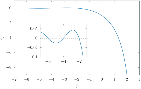
Figure 2: The rest-frame finite-volume coefficients $c_{j}$ as a function of $j$. The inset panel is a zoom on the small oscillations in the $-7\leq j\leq-1$ region, with zeros on even negative integers.

$j$	$c_{j}$
$-5$	$-0.02587$
$-3$	$0.04118$
$-1$	$-0.26660$
$0$	$-1$
$1$	$-2.83730$
$2$	$-8.91363$

Table 1: Values of selected zero-velocity finite-volume coefficients.

III.3.2 Moving-frame coefficients and rotational symmetry breaking effects

In a finite cubic volume, the rotational symmetry group is broken down to the cubic symmetry group. Therefore, at non-zero velocity, finite-volume effects will depend on the direction of the vector $\mathbf{v}$. Upon inspecting the results of the previous section, it becomes clear that the rotational symmetry breaking effects will be encoded in the dependence of the $c_{2,1}(\mathbf{v})$ coefficient on the velocity direction. This can be explored in more detail by means of a spherical harmonic analysis of the angular dependence of $c_{2,1}(\mathbf{v})$. Consider the spherical expansion

$$\frac{1}{|\mathbf{n}|^{j}(1-\mathbf{v}\cdot\hat{\mathbf{n}})^{k}}=\frac{1}{|\mathbf{n}|^{j}}\sum_{l=0}^{+\infty}\sum_{m=-l}^{l}a_{klm}(\mathbf{v})Y_{lm}(\theta_{\mathbf{n}},\phi_{\mathbf{n}})\,,$$ (73)

where $Y_{lm}$ is the normalized spherical harmonic

$$Y_{lm}(\theta,\phi)=\sqrt{\frac{2l+1}{4\pi}}\sqrt{\frac{(l-m)!}{(l+m)!}}P_{lm}[\cos(\theta)]e^{im\phi}\,,$$ (74)

with $P_{lm}$ the associated Legendre polynomial. Moreover, $\theta_{\mathbf{n}}$ and $\phi_{\mathbf{n}}$ are the angular spherical coordinates of $\mathbf{n}$,

$$\hat{\mathbf{n}}=\left(\sin(\theta_{\mathbf{n}})\cos(\phi_{\mathbf{n}}),\sin(\theta_{\mathbf{n}})\sin(\phi_{\mathbf{n}}),\cos(\theta_{\mathbf{n}})\right)\,.$$ (75)

Rotational symmetry requires that the integrals over $\mathbf{n}$ of the terms in eq. 73 vanish except for the $l=0$ term, allowing the $c_{j,k}(\mathbf{v})$ coefficients in eq. 42 to be written as

$$c_{j,k}(\mathbf{v})=A_{k}(|\mathbf{v}|)c_{j}+\sum_{l=1}^{+\infty}\sum_{m=-l}^{l}a_{klm}(\mathbf{v})y_{jlm}\,,$$ (76)

where

$$A_{k}(\beta) =\frac{1}{2}\int_{-1}^{1}\frac{\mathrm{d}x}{(1-\beta x)^{k}}=\frac{1}{2\beta(k-1)}\left[\left(\frac{1}{1-\beta}\right)^{k-1}-\left(\frac{1}{1+\beta}\right)^{k-1}\right],$$ (77)

and

$$y_{jlm} =\Delta_{\mathbf{n}}^{\prime}[|\mathbf{n}|^{-j}Y_{lm}(\theta_{\mathbf{n}},\phi_{\mathbf{n}})]=\operatorname*{\sideset{}{{}^{\prime}}{\sum}}_{\mathbf{n}}\frac{Y_{lm}(\theta_{\mathbf{n}},\phi_{\mathbf{n}})}{|\mathbf{n}|^{j}}\,.$$ (78)

The coefficients $y_{jlm}$ are given in terms of the generalized zeta function from Ref. (Luscher, 1986) through the relation

$$y_{jlm}=\sqrt{\frac{4\pi}{2l+1}}Z_{lm}\left(\frac{j-l}{2},\mathbf{0}\right)\,.$$ (79)

The expression in eq. 76 is the main result of this section, and shows that the $c_{j,k}(\mathbf{v})$ coefficients, up to rotational symmetry breaking effects, are proportional to $c_{j}$ by a known factor depending only on the magnitude of the velocity $\mathbf{v}$. Rotational-symmetry breaking effects enter through the higher multipole contributions $a_{klm}(\mathbf{v})$. The function $A_{k}(\beta)$ has the limits

$$A_{k}(0)=1\qquad\text{and}\qquad A_{1}(\beta)=\frac{\operatorname{arctanh}(\beta)}{\beta}\,.$$ (80)

In the case that is relevant to QED finite-volume corrections, the rotational symmetry approximation $\overline{c}_{2,1}(|\mathbf{v}|)$ of $c_{2,1}(\mathbf{v})$ is given by

$$\overline{c}_{2,1}(|\mathbf{v}|)=\frac{\pi c_{1}}{|\mathbf{v}|}\operatorname{arctanh}(|\mathbf{v}|)\,,$$ (81)

where the presence of the rapidity $\operatorname{arctanh}(|\mathbf{v}|)$ is noted. In fig. 3, the exact value of $c_{2,1}(\mathbf{v})$ is compared to $\overline{c}_{2,1}(|\mathbf{v}|)$ for sample velocity orientations.

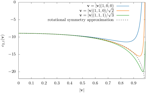
Figure 3: The finite-volume coefficient $c_{2,1}(\mathbf{v})$ as a function of the velocity norm for typical orientations of the velocity compared to the rotational symmetry approximation given in eq. 81. The values of $c_{2,1}(\mathbf{v})$ displayed here have been computed numerically using the techniques described in appendix B.

The rotational symmetry approximation appears to be very good up to velocities $|\mathbf{v}|\sim 0.5$. At ultra-relativistic velocities, the rotational symmetry breaking effects dominate. As it is proven in details in appendix C, $a_{klm}(\mathbf{v})=\mathcal{O}(|\mathbf{v}|^{l})$. Using this property, eq. 73 can be interpreted as a power expansion in $|\mathbf{v}|$, explaining the ultra-relativistic behavior.

IV Infrared improvement of the $\mathrm{QED}_{\mathrm{L}}$ theory

$\mathrm{QED}_{\mathrm{L}}$ is a minimal choice to implement QED in a finite volume in which photon zero-mode singularities are regulated by introducing a particular form of non-locality in space while preserving locality in time. Non-minimal choices are possible as well and lead to different approaches to the infinite-volume limit. Such extra non-localities can be tuned to remove or suppress finite-volume effects. This approach has similarities to Symanzik’s improvement program that subtracts discretization effects in lattice gauge theories. Given this, we call the method detailed below infrared improvement.

Although knowledge of the analytic form of leading finite-volume effects in $\mathrm{QED}_{\mathrm{L}}$ in principle suffices to subtract them out in obtaining the infinite-volume values of quantities, it is still advantageous to carry out numerical calculations in an improved scheme. Consider a situation in which the finite-volume value is significantly different than the infinite-volume value, which can be the case in relatively small volumes. Then the computational resources required to accurately perform the required subtraction will be significant, prohibiting precision calculations of some quantities in $\mathrm{QED}_{\mathrm{L}}$. As shown below, a relatively general infrared improvement of $\mathrm{QED}_{\mathrm{L}}$ leads to mass corrections of the order of sub-percent level even at small volumes, which would be comparable to or smaller than other systematics in most state-of-the-art numerical calculations. Similar limitations are encountered in studies of moments of parton distribution functions of hadrons with lattice QCD, where using conventional methods, contributions from lower-dimension operators dominate over the continuum-limit contributions, requiring new ideas that implement an improvement procedure in such calculations, see e.g. Refs. (Davoudi and Savage, 2012; Detmold and Lin, 2006; Monahan and Orginos, 2015). Similar ideas have been suggested in taking advantage of numerical simulations with multiple center-of-mass boosts or boundary conditions to find optimal combination of quantities that suppress finite-volume effects in cases where the target quantity is small compared with other scales in the system, such as the deuteron binding energy or the S-wave/D-wave mixing in the isosinglet two-nucleon system (Davoudi and Savage, 2011; Briceno et al., 2013, 2014).

An additional motivation for an infrared-improved $\mathrm{QED}_{\mathrm{L}}$ concerns studies of systems with multiple charged hadrons. For example, as is demonstrated in Ref. (Beane and Savage, 2014), the power-law corrections to the mass of charged particles modify the kinematics of $2\to 2$ scattering processes, requiring keeping track of this change in subsequent calculations. Starting out with the incoming and outgoing hadrons that are already close to their infinite-volume mass simplifies the formalism that extracts scattering amplitudes from energy spectra. Additionally, the relatively general improvement scheme introduced in section IV.2.2 suggests that such a single-body improvement may lead to an improvement in finite-volume corrections in two and multi-hadron observables, a statement that will be investigated in future studies.

IV.1 General concept

Consider the $\mathrm{QED}_{\mathrm{L}}$ action described in section II, written in momentum space,

$$S_{L}[\hat{A}_{\mu}]=\frac{1}{2L^{3}}\int\frac{\mathrm{d}k_{0}}{2\pi}\operatorname*{\sideset{}{{}^{\prime}}{\sum}}_{\mathbf{k}\in\hat{\mathbb{T}}^{3}}\hat{A}_{\mu}(k)^{*}\Omega_{\mu\nu}(k)\hat{A}_{\nu}(k)\,,$$ (82)

where the decoupled spatial zero-mode is removed and the kernel $\Omega_{\mu\nu}(k)$ is given by

$$\Omega_{\mu\nu}(k)=\delta_{\mu\nu}k^{2}-k_{\mu}k_{\nu}\,.$$ (83)

Note that the gauge has not yet been fixed. In momentum space, gauge invariance can be summarized by the identity

$$k_{\mu}\Omega_{\mu\nu}(k)=0\,,$$ (84)

so the tensor $\Omega_{\mu\nu}(k)$ is transverse for any $k$. Now let us define the infrared-improved action through

$$S_{L,w}[\hat{A}_{\mu}]=\frac{1}{2L^{3}}\int\frac{\mathrm{d}k_{0}}{2\pi}\operatorname*{\sideset{}{{}^{\prime}}{\sum}}_{\mathbf{k}\in\hat{\mathbb{T}}^{3}}\frac{\hat{A}_{\mu}(k)^{*}\Omega_{\mu\nu}(k)\hat{A}_{\nu}(k)}{1+w_{|\mathbf{n}|^{2}}}\,,$$ (85)

where $\mathbf{n}=\frac{L}{2\pi}\mathbf{k}$ and the $w_{|\mathbf{n}|^{2}}$ are real coefficients which are non-zero only for a finite number of values of $|\mathbf{n}|$. Because of this property, the contributions from the $w_{|\mathbf{n}|^{2}}$ vanish in the infinite-volume limit. To preserve the positivity of the action, an additional constraint, $w_{|\mathbf{n}|^{2}}>-1$ is placed on the coefficients for any $\mathbf{n}$. As the only effect of introducing $w_{|\mathbf{n}|^{2}}$ coefficients is to reweight the action kernel, eq. 84 still holds and the theory remains gauge invariant. Gauge fixing and integrating out the redundant gauge degree of freedom results in a kernel that is an invertible matrix $\overline{\Omega}_{\mu\nu}(k)$, e.g. $\delta_{\mu\nu}k^{2}$ in Feynman gauge. In the Euclidean quantum field theory associated with eq. 85, the momentum-space photon propagator is

$$\hat{D}_{\mu\nu}^{(L,w)}(k) =(1+w_{|\mathbf{n}|^{2}})\overline{\Omega}^{-1}_{\mu\nu}(k)=(1+w_{|\mathbf{n}|^{2}})\hat{D}_{\mu\nu}^{(L)}(k)\,,$$ (86)

where $\hat{D}_{\mu\nu}^{(L)}(k)$ is the $\mathrm{QED}_{\mathrm{L}}$ photon propagator. The weight functions $w_{|\mathbf{n}|^{2}}$ modify the residue of the photon propagator near its pole, and as was demonstrated in section III, the coefficients of the large-volume expansion depend on this residue. The strategy of the infrared improvement is to tune a finite number of $w_{|\mathbf{n}|^{2}}$ to reduce the finite-volume effects.

More explicitly, because of its discrete and finite nature, multiplying the photon propagator by $1+w_{|\mathbf{n}|^{2}}$ does not change the singularity structure of the contour integral in eq. 36. Therefore, the general formulas eqs. 46, 40 and 47 still holds by replacing the coefficients $c_{j,k}(\mathbf{v})$ and $\xi_{j,k,l}(p)$ by

$$c_{j,k}^{(w)}(\mathbf{v}) =c_{j,k}(\mathbf{v})+\operatorname*{\sideset{}{{}^{\prime}}{\sum}}_{\mathbf{n}}\frac{w_{|\mathbf{n}|^{2}}}{|\mathbf{n}|^{j}(1-\mathbf{v}\cdot\hat{\mathbf{n}})^{k}}\,,$$ (87)

$$\xi_{j,k,l}^{(w)}(p) =\xi_{j,k,l}(p)+\operatorname*{\sideset{}{{}^{\prime}}{\sum}}_{\mathbf{n}}\frac{w_{|\mathbf{n}|^{2}}f_{l}(\hat{\mathbf{n}},p)}{|\mathbf{n}|^{j}(1-\mathbf{v}\cdot\hat{\mathbf{n}})^{k}}\,,$$ (88)

respectively. We now discuss in detail different strategies to tune the weights $w_{|\mathbf{n}|^{2}}$ for the self-energy functions.

IV.2 Infrared improvement of the self-energy

As an example, let us consider the case of the on-shell scalar self-energy, for which the finite-volume contribution was derived in section III.2. From what was described in the previous section, in the infrared-improved theory one obtains

$$\Delta\omega_{0}(\mathbf{p})^{2}=m^{2}q^{2}\left\{\frac{1}{\gamma(|\mathbf{v}|)}\frac{c_{2,1}^{(w)}(\mathbf{v})}{4\pi^{2}\mu}+\frac{c_{1}^{(w)}}{2\pi\mu^{2}}-\left[\frac{1}{\gamma(|\mathbf{v}|)}-\frac{1}{\gamma(|\mathbf{v}|)^{3}}\right]\frac{c_{0}^{(w)}}{2\mu^{3}}+\cdots\right\}\,.$$ (89)

It is useful to define the finite sum,

$$\sigma_{k,N}(\mathbf{v})\equiv\sum_{|\mathbf{n}|^{2}=N}(1-\mathbf{v}\cdot\hat{\mathbf{n}})^{-k}\,,$$ (90)

from which the coefficients $c_{j,k}^{(w)}(\mathbf{v})$ become

$$c_{j,k}^{(w)}(\mathbf{v})=c_{j,k}(\mathbf{v})+\sum_{N=1}^{+\infty}\frac{w_{N}}{N^{\frac{j}{2}}}\sigma_{k,N}(\mathbf{v})\,.$$ (91)

Note that the sum in eq. 90 only runs over integer vectors $\mathbf{n}$ with length $N$. For zero velocity, $\sigma_{k,N}(\mathbf{v})$ becomes equal to $r_{3}(N)$, the number of integer solutions to the equation $x^{2}+y^{2}+z^{2}=N$. The values of this function which are relevant here are

$$r_{3}(1)=6,\qquad\text{and}\qquad r_{3}(2)=12\,.$$ (92)

It is interesting to consider the possibility of completely canceling finite-volume contributions up to a given order in the $\frac{1}{L}$ expansion. Unfortunately, this is not always possible to achieve and does not have a clear qualitative benefit in typical physical scenarios, as is shown below for the case of the mass. One may therefore explore the possibility of approximately canceling the sum of several orders in the $\frac{1}{L}$ expansion in a given reference volume. For the finite-volume corrections to a charged particle mass, we find that this strategy is generally more feasible and allows for a reduction in these effects below the percent level for volumes typically used in lattice QCD+QED calculations.

IV.2.1 $\operatorname{\mathcal{O}}(\frac{1}{L})$ and $\operatorname{\mathcal{O}}(\frac{1}{L^{2}})$ improvements

To completely remove the $\operatorname{\mathcal{O}}(\frac{1}{L})$ finite-volume effects given in  eqs. 89 and 91, one needs to solve the condition $c_{j,k}^{(w)}(\mathbf{v})=0$. A minimal choice that satisfies this is

$$w_{1}=-\frac{c_{2,1}(\mathbf{v})}{\sigma_{1,1}(\mathbf{v})},\qquad\text{or}\qquad w_{1}=-\frac{\pi}{6}c_{1}\text{\leavevmode\nobreak\ \leavevmode\nobreak\ for\leavevmode\nobreak\ \leavevmode\nobreak\ }\mathbf{v}=0\,,$$ (93)

and $w_{N}=0$ for all $N>1$. This weight function modifies the $\operatorname{\mathcal{O}}(\frac{1}{L^{2}})$ and $\operatorname{\mathcal{O}}(\frac{1}{L^{3}})$ coefficients to become

$$c_{1}^{(w)}=c_{1}-6\frac{c_{2,1}(\mathbf{v})}{\sigma_{1,1}(\mathbf{v})},\qquad\text{and}\qquad c_{0}^{(w)}=-1-6\frac{c_{2,1}(\mathbf{v})}{\sigma_{1,1}(\mathbf{v})}\,.$$ (94)

Numerical values for the $w_{|\mathbf{n}|^{2}}$ and $c_{j}^{(w)}$ presented in this section, and in the following, are summarized in table 2.

The $\operatorname{\mathcal{O}}(\frac{1}{L^{2}})$-improved coefficients are given by  eq. 91 through the linear system

$$c_{2,1}(\mathbf{v})+w_{1}\ \sigma_{1,1}(\mathbf{v})+\frac{1}{2}\ w_{2}\ \sigma_{1,2}(\mathbf{v}) =0\,,$$ (95)

$$c_{1}+6w_{1}+6\sqrt{2}w_{2} =0\,,$$ (96)

which gives

$$w_{1} =\frac{c_{1}\sigma_{1,2}(\mathbf{v})-12\sqrt{2}c_{2,1}(\mathbf{v})}{6[2\sqrt{2}\sigma_{1,1}(\mathbf{v})-\sigma_{1,2}(\mathbf{v})]}$$ (97)

$$\text{or}\qquad w_{1} =-\frac{1}{6}(1+\sqrt{2})(\sqrt{2}\pi-1)c_{1}=3.93053406\dots\text{\leavevmode\nobreak\ \leavevmode\nobreak\ for\leavevmode\nobreak\ \leavevmode\nobreak\ }\mathbf{v}=0\,,$$ (98)

$$w_{2} =\frac{6c_{2,1}(\mathbf{v})-c_{1}\sigma_{1,1}(\mathbf{v})}{3[2\sqrt{2}\sigma_{1,1}(\mathbf{v})-\sigma_{1,2}(\mathbf{v})]}$$ (99)

$$\text{or}\qquad w_{2} =\frac{1}{6}(1+\sqrt{2})(\pi-1)c_{1}=-2.44492857\dots\text{\leavevmode\nobreak\ \leavevmode\nobreak\ for\leavevmode\nobreak\ \leavevmode\nobreak\ }\mathbf{v}=0\,,$$ (100)

where the least number of coefficients that allow a full cancellation of $\operatorname{\mathcal{O}}(\frac{1}{L})$ and $\operatorname{\mathcal{O}}(\frac{1}{L^{2}})$ effects are considered. In the rest frame we obtain $w_{2}\leq-1$ which violates the positivity of the action in  eq. 85. Similar occurrences of the same issue arising in other situations were found in attempting to exactly cancel the finite-volume effect up to a given order, warranting investigations into other forms of constraints on the weight factors $w_{|\mathbf{n}|^{2}}$. Note that at this order, the finite-volume corrections to the mass of spin-0 and spin-$\frac{1}{2}$ particles are the same and the same weight factors apply to both cases.

The $\operatorname{\mathcal{O}}(\frac{1}{L})$-improved finite-volume corrections to the mass are presented in fig. 4. The improved effects are smaller for large values of $mL$, but are, in fact, larger than in $\mathrm{QED}_{\mathrm{L}}$ for values around $mL=4$, making the benefit of this improvement strategy limited. This provides an additional motivation to look for better improvement prescriptions.

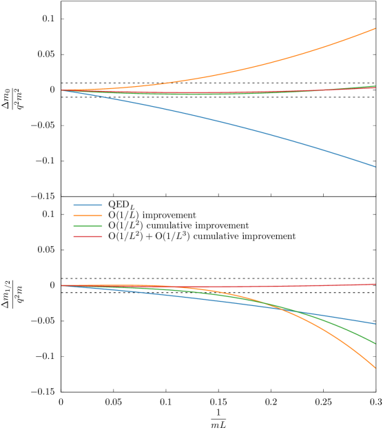
Figure 4: Relative finite-volume contributions to charged-particle masses in $\mathrm{QED}_{\mathrm{L}}$, and the improved versions described in section IV.2. The upper panel shows corrections to the spin-0 mass squared, while the lower panel shows the spin-$\frac{1}{2}$ mass contribution, both in units of $q^{2}m$. The dashed lines indicate the regions within which the finite-volume contributions are below $1\%$ relative to the electromagnetic corrections to the mass.

Improvement	$w_{1}$	$w_{2}$	$c_{2}^{(w)}$	$c_{1}^{(w)}$	$c_{0}^{(w)}$
None	$0$	$0$	$-8.91363292$	$-2.83729748$	$-1$
$\operatorname{\mathcal{O}}(\frac{1}{L})$	$1.48560549$	$0$	$0$	$6.07633544$	$7.91363292$
cumulative $\operatorname{\mathcal{O}}(\frac{1}{L^{2}})$	$0.86681632$	$0$	$-3.71273496$	$2.36360048$	$4.20089796$
cumulative $\operatorname{\mathcal{O}}(\frac{1}{L^{3}})$	$0.52392582$	$0$	$-5.77007797$	$0.30625747$	$2.14355495$
cumulative $\operatorname{\mathcal{O}}(\frac{1}{L^{2}})+\operatorname{\mathcal{O}}(\frac{1}{L^{3}})$	$2.04145881$	$-0.93739607$	$-2.28925650$	$1.45738594$	$0$

Table 2: Summary of improvement weight factors and finite-volume coefficients according to the improvement prescriptions for the mass of charged hadrons described in section IV.2. Values from cumulative improvement prescriptions are given for the reference scale $\mu_{0}=mL_{0}=4$.

IV.2.2 Cumulative improvement

From what was derived so far, it is reasonable to assume, even without prior knowledge of the finite-volume coefficients, that $\Delta\omega_{0}(\mathbf{p})^{2}/m^{2}$ has a power expansion in

$$\frac{c_{3-j}^{(w)}}{(2\pi)^{3-j}\mu^{j}}$$ (101)

with ${\cal O}\left(1\right)$ coefficients. Consequently, one possible strategy to circumvent the positivity issue encountered in the previous section is to tune the improvement weights $w_{n}$ to obtain

$$\frac{c_{2}^{(w)}}{4\pi^{2}\mu_{0}}+\frac{c_{1}^{(w)}}{2\pi\mu_{0}^{2}}=0\,,$$ (102)

for a reference volume $\mu_{0}=mL_{0}$. This is achievable by a minimal choice

$$w_{1}=-\frac{\pi}{6}\frac{2+\mu_{0}}{2\pi+\mu_{0}}c_{1}\,.$$ (103)

In lattice QCD+QED calculations, typical values for $\mu$ are: $\mu\gtrsim 4$. For any positive $\mu_{0}$, eq. 103 gives $w_{1}>-1$, which does not violate the positivity of the action. Numerical values for $w_{1}$ and the $c_{j}^{(w)}$ coefficients are given in table 2. Similarly, combinations of the three first orders can be suppressed by solving

$$\frac{c_{2}^{(w)}}{4\pi^{2}\mu_{0}}+\frac{c_{1}^{(w)}}{2\pi\mu_{0}^{2}}+\frac{c_{0}^{(w)}}{\mu_{0}^{3}}=0\,,$$ (104)

which gives

$$w_{1}=\frac{\pi}{6}\frac{4\pi-2\mu_{0}c_{1}-\mu_{0}^{2}c_{1}}{4\pi^{2}+2\pi\mu_{0}+\mu_{0}^{2}}\,.$$ (105)

Finally, eqs. 102 and 104 can be simultaneously solved using the two weights $w_{1}$ and $w_{2}$ to obtain

$$w_{1} =\frac{1}{6}\frac{2\sqrt{2}\pi+\mu_{0}+4\pi c_{1}+2\pi\mu_{0}c_{1}}{2\sqrt{2}\pi-4\pi-\mu_{0}},$$ (106)

$$w_{2} =-\frac{1}{6}\frac{2\pi+\mu_{0}+2\pi c_{1}+\pi\mu_{0}c_{1}}{2\sqrt{2}\pi-4\pi-\mu_{0}}\,.$$ (107)

The finite-volume effects in the cumulative improvement at the reference scale $\mu_{0}=4$ are shown in fig. 4. The $\operatorname{\mathcal{O}}(\frac{1}{L^{2}})+\operatorname{\mathcal{O}}(\frac{1}{L^{3}})$ cumulative improvement is efficient, producing subpercent relative finite-volume corrections for any $mL>4$ in the masses of both spin-$0$ and spin-$\frac{1}{2}$ charged particles.

IV.2.3 Universality of the procedure

One legitimate worry about the improvement procedure is its observable dependence. The quality of the improvement is, in principle, determined by the target observable and could actually enhance finite-volume effects on other observables. However, the cumulative improvement scheme is based on minimizing the first terms in the volume expansion assuming some naturalness of the power expansion driven by eq. 101. Further investigations are needed to determine the extent to which this is a good assumption. This likely requires generalizing the formal derivation in appendix A to arbitrary one-loop diagram for leading-order electromagnetic corrections. Such a calculation is beyond the scope of the present paper. Nevertheless, one of the interesting aspects of the procedure presented here is to emphasis the arbitrariness in the choice of scheme for subtracting the photon zero-mode. As explained in section II, the standard $\mathrm{QED}_{\mathrm{L}}$ scheme is minimal with respect to locality in time, but there is no reason for it to be optimal for finite-volume effects. The improvement procedure discussed here gives a practical example of the potential benefits of modifying this prescription.

V Numerical study through simulations of lattice scalar QED

As a laboratory to test ideas presented in the previous sections and to allow for checks of the finite-volume relations, we have performed a dedicated numerical lattice QED study to compute the self-energy of a fundamental charged scalar particle in a finite volume with periodic boundary conditions.

V.1 Lattice scalar $\mathrm{QED}_{\mathrm{L}}$

Consider a finite 4-dimensional lattice, $\Lambda^{4}$, with a lattice spacing $a$, temporal extent $T=aN_{T}$ and spatial extent $L=aN_{L}$. It is convenient to define a translation operator in the $\mu$ direction

$$\tau_{\mu}f(x)=f(x+a\hat{\mu})\,,$$ (108)

where $f$ is an arbitrary function of coordinates and $\hat{\mu}$ is the unit vector in direction $\mu$, using which discrete derivatives and covariant derivatives can be defined,

$$\delta_{\mu} =a^{-1}(\tau_{\mu}-1),$$ (109)

$$\delta^{*}_{\mu} =a^{-1}(1-\tau_{-\mu}),$$ (110)

$$\delta^{2} ={\textstyle\sum_{\mu}}\delta_{\mu}\delta^{*}_{\mu}\,$$ (111)

$$\nabla_{\mu} =a^{-1}(e^{iaqA_{\mu}}\tau_{\mu}-1)=e^{iaqA_{\mu}}\delta_{\mu}+a^{-1}(e^{iaqA_{\mu}}-1)\,,$$ (112)

$$\nabla^{*}_{\mu} =a^{-1}(1-\tau_{-\mu}e^{-iaqA_{\mu}})=\delta^{*}_{\mu}e^{-iaqA_{\mu}}+a^{-1}(1-e^{-iaqA_{\mu}})\,,$$ (113)

$$\nabla^{2} ={\textstyle\sum_{\mu}}\nabla_{\mu}\nabla^{*}_{\mu}\,,$$ (114)

where $A_{\mu}$ is the $\operatorname{U}(1)$ gauge potential and $q$ is the charge of the scalar particle.

V.1.1 Lattice action and observables

On such a lattice, the QED action for a scalar complex field in Feynman gauge is given by

$$S[\phi,A_{\mu}]=S_{\phi}[\phi,A_{\mu}]+S_{\mathrm{Feyn.}}[A_{\mu}]\,,$$ (115)

where the matter term is

$$S_{\phi}[\phi,A_{\mu}]=a^{4}\sum_{x\in\Lambda^{4}}\left\{{\textstyle\sum_{\mu}}|\nabla_{\mu}\phi(x)|^{2}+m^{2}|\phi(x)|^{2}\right\}=a^{4}\sum_{x\in\Lambda^{4}}\phi(x)\Delta\phi(x)^{*}\,,$$ (116)

with $\Delta=-\nabla^{2}+m^{2}$. The gauge action takes the form

$$S_{\mathrm{Feyn.}}[A_{\mu}]=a^{4}\sum_{x\in\Lambda^{4}}\left\{\frac{1}{4}{\textstyle\sum_{\mu,\nu}}F_{\mu\nu}(x)^{2}+\frac{1}{2}{\textstyle\sum_{\mu}}[\delta_{\mu}A_{\mu}(x)]^{2}\right\}=-\frac{a^{4}}{2}\sum_{x\in\Lambda^{4}}A_{\mu}(x)\delta^{2}A_{\mu}(x)\,,$$ (117)

where $F_{\mu\nu}=\delta_{\mu}A_{\nu}-\delta_{\nu}A_{\mu}$.

In this theory, a scalar observable $O[\phi,\phi^{*}]$ has the expectation value

$$\braket{O}=\frac{1}{\mathscr{Z}_{\mathrm{L}}}\int\mathcal{D}A_{\mu}\,\mathcal{D}\phi\,\mathcal{D}\phi^{*}\,O[\phi,\phi^{*}]\exp(-S_{L}[\phi,A_{\mu}])\,,$$ (118)

where $\mathscr{Z}_{\mathrm{L}}$ is the partition function, and the index $L$ indicates use of the the $\mathrm{QED}_{\mathrm{L}}$ prescription described in section II, corresponding to the condition

$$a^{3}\sum_{\mathbf{x}\in\Lambda^{3}}A_{\mu}(t,\mathbf{x})=0\,,$$ (119)

where $\Lambda^{3}$ is the spatial sub-lattice. Since the action in  eq. 116 is quadratic in $(\phi,\phi^{*})$, the integration over the scalar fields can be performed analytically,

$$\braket{O}=\frac{1}{\mathscr{Z}_{\mathrm{L}}}\int\mathcal{D}A_{\mu}\,O_{\mathrm{Wick}}[\Delta^{-1}]\det(\Delta)^{-\frac{1}{2}}\exp(-S_{\mathrm{Feyn.,L}}[A_{\mu}])\,,$$ (120)

where $O_{\mathrm{Wick}}$ is the function arising from Wick contractions of matter fields in operator $O$. Due to the symmetry $A_{\mu}\mapsto-A_{\mu}$ of the action $S_{\mathrm{Feyn.,L}}$, any contributions that are odd in the charge $q$ are absent from expectation values. To obtain the leading order, $\operatorname{\mathcal{O}}(q^{2})$, corrections to $\braket{O}$, it is therefore sufficient to use the quenched theory, i.e. to set $\det(\Delta)=1$. eq. 120 can then be evaluated using Monte-Carlo techniques by computing the observable $O_{\mathrm{Wick}}[\Delta^{-1}]$ for $A_{\mu}$ fields sampled from the Gaussian distribution $\mathcal{D}A_{\mu}\,\exp(-S_{\mathrm{Feyn.,L}}[A_{\mu}])$.

V.1.2 Scalar propagator

The terms in the expansion of the lattice Laplacian $\nabla^{2}$ in leading powers of $q$ are

$$\Delta=\Delta_{0}+q\Delta_{1}+q^{2}\Delta_{2}+\operatorname{\mathcal{O}}(q^{3})\,,$$ (121)

with

$$\Delta_{0} =-a^{-2}(\tau_{\mu}+\tau_{-\mu}-2)\,,$$ (122)

$$\Delta_{1} =-ia^{-1}\,{\textstyle\sum_{\mu}}(A_{\mu}\tau_{\mu}-\tau_{-\mu}A_{\mu})\,,$$ (123)

$$\Delta_{2} =\frac{1}{2}\,{\textstyle\sum_{\mu}}(A_{\mu}^{2}\tau_{\mu}+\tau_{-\mu}A_{\mu}^{2})\,.$$ (124)

The scalar propagator is then given by

$$\Delta^{-1}=\Delta_{0}^{-1}-q\Delta_{0}^{-1}\Delta_{1}\Delta_{0}^{-1}+q^{2}\Delta_{0}^{-1}\Delta_{1}\Delta_{0}^{-1}\Delta_{1}\Delta_{0}^{-1}-q^{2}\Delta_{0}^{-1}\Delta_{2}\Delta_{0}^{-1}+\operatorname{\mathcal{O}}(q^{3})\,,$$ (125)

which can be diagramatically represented as

$$\raisebox{-8.0pt}{\includegraphics{feyn_prop_full.pdf}}=\raisebox{1.0pt}{\includegraphics{feyn_prop_free.pdf}}-q\,\raisebox{-1.0pt}{\includegraphics{feyn_prop_d1.pdf}}+q^{2}\,\raisebox{-1.0pt}{\includegraphics{feyn_prop_d12.pdf}}-q^{2}\,\raisebox{-2.0pt}{\includegraphics{feyn_prop_d2.pdf}}\,.$$ (126)

Here, the line, cross and square vertices represent the free scalar propagator, an insertion of $\Delta_{1}$ and an insertion of $\Delta_{2}$, respectively.

One may define the lattice Fourier transform,

$$[\mathcal{F}f(x)](k)=\widetilde{f}(k)=a^{4}\sum_{x\in\Lambda^{4}}f(x)e^{-ik\cdotp x}$$ (127)

and its inverse,

$$[\mathcal{F}^{-1}\widetilde{f}(k)](x)=f(x)=\frac{1}{TL^{3}}\sum_{k\in\hat{\Lambda}^{4}}\widetilde{f}(k)e^{ik\cdotp x}$$ (128)

to represent the scalar propagator in momentum space. The free propagator is given by

$$\Delta_{0}^{-1}=\mathcal{F}^{-1}G\mathcal{F}$$ (129)

where $G$ is the diagonal, momentum space operator

$$G(p)=\frac{1}{\hat{p}^{2}+m^{2}}$$ (130)

with the lattice momentum $\hat{p}_{\mu}=\frac{2}{a}\sin\left(\frac{ap_{\mu}}{2}\right)$. Further, using eqs. 123 and 124, it is straightforward to show that in momentum space

$$\raisebox{-1.0pt}{\includegraphics{feyn_prop_d1.pdf}}=\Delta_{0}^{-1}\Delta_{1}\Delta_{0}^{-1} =-ia^{-1}\sum_{\mu}\mathcal{F}^{-1}(G\mathcal{F}A_{\mu}\mathcal{F}^{-1}\psi_{\mu}G-G\psi_{\mu}^{*}\mathcal{F}A_{\mu}\mathcal{F}^{-1}G)\mathcal{F}\,,$$ (131)

$$\raisebox{-2.0pt}{\includegraphics{feyn_prop_d2.pdf}}=\Delta_{0}^{-1}\Delta_{2}\Delta_{0}^{-1} =\frac{1}{2}\sum_{\mu}\mathcal{F}^{-1}(G\mathcal{F}A_{\mu}^{2}\mathcal{F}^{-1}\psi_{\mu}G+G\psi_{\mu}^{*}\mathcal{F}A_{\mu}^{2}\mathcal{F}^{-1}G)\mathcal{F}\,,$$ (132)

where $\psi_{\mu}(p)=e^{iap_{\mu}}$. These expressions are rather formal depictions of what could be obtained through the Feynman rules of lattice scalar QED in a background electromagnetic field. In this form, it is clear that the $\operatorname{\mathcal{O}}(q^{2})$ expansion of the inverse operator $\Delta^{-1}$ in a given stochastic field $A_{\mu}(x)$ can be computed solely using a fast Fourier transform (FFT) algorithm. This approach has two important advantages compared to more conventional approaches that use iterative inverters, such as the conjugate gradient algorithm. First, the complexity of performing a FFT is independent of the mass of the particle, and second, it scales as $V\log(V)$ where $V=TL^{3}$, making it of practical use for large-volume studies.

V.2 On-shell self-energy from Euclidean-time correlators

The primary output of lattice QED simulations performed are time correlators, from which we will obtain the particle’s self-energy. The on-shell point is defined through an analytic continuation of $\Sigma(p)$ to imaginary $p_{0}$. As is usual in Euclidean field theory, this point is accessed through the large-time behavior of relevant correlation functions. The 2-point function of the charged scalar particle in the time-momentum representation is given by

$$C(t,\mathbf{p})=a^{3}\sum_{\mathbf{x}\in\Lambda^{3}}\braket{\mathrm{T}[\phi(t,\mathbf{x})\phi(0)^{\dagger}]}e^{-i\mathbf{p}\cdotp\mathbf{x}}\,.$$ (133)

At small electric charges, this function can be decomposed into the tree level and first-order electromagnetic corrections

$$C(t,\mathbf{p})=C_{0}(t,\mathbf{p})+C_{1}(t,\mathbf{p})\,,$$ (134)

which, in practice, are obtained from the diagrams in eq. 126. The full spectral representation of $C_{1}(t,\mathbf{p})$ on a continuous space-time is presented here, while the lattice equivalent of this result, which is used to analyze computed lattice correlators, is obtained in appendix D.

The function $C_{0}(t,\mathbf{p})$ is the free scalar propagator, and is given by

$$C_{0}(t,\mathbf{p})=\int\frac{\mathrm{d}p_{0}}{2\pi}\frac{e^{ip_{0}t}}{p^{2}+m^{2}}=\frac{e^{-\omega(\mathbf{p})|t|}}{2\omega(\mathbf{p})}\,.$$ (135)

The self-energy function $\Sigma(p)$ is defined by the amputated first order corrections

$$C_{1}(t,\mathbf{p})=\int\frac{\mathrm{d}p_{0}}{2\pi}\frac{\Sigma(p)}{(p^{2}+m^{2})^{2}}e^{ip_{0}t}\,,$$ (136)

as discussed in section III.1.1. It is defined through eqs. 26 and 30, and is given by

$$\Sigma(p)=\frac{q^{2}}{L^{3}}\operatorname*{\sideset{}{{}^{\prime}}{\sum}}_{\mathbf{k}\in\mathrm{BZ}(L)}\int\frac{\mathrm{d}k_{0}}{2\pi}\left\{\frac{4}{k^{2}}-\frac{(2p-k)^{2}}{k^{2}[(p-k)^{2}+m^{2}]}\right\}\,,$$ (137)

The $k_{0}$ integral can be performed to give

$$\Sigma(p)=\frac{q^{2}}{L^{3}}\operatorname*{\sideset{}{{}^{\prime}}{\sum}}_{\mathbf{k}\in\mathrm{BZ}(L)} \left\{\frac{2}{|\mathbf{k}|}\right.+\frac{4p_{0}^{2}+\mathbf{k}^{2}+(2\mathbf{p}-\mathbf{k})^{2}}{2|\mathbf{k}|[p_{0}^{2}+\omega_{\gamma}(\mathbf{p},\mathbf{k})^{2}]}$$

$$\quad+\left.\frac{p_{0}^{2}+\omega(\mathbf{p}-\mathbf{k})^{2}+(2\mathbf{p}-\mathbf{k})^{2}}{2\omega(\mathbf{p}-\mathbf{k})[p_{0}^{2}+\omega_{\gamma}(\mathbf{p},\mathbf{k})^{2}]}\right\}\,,$$ (138)

which has the expected poles at $p_{0}=\pm i\omega_{\gamma}(\mathbf{p},\mathbf{k})$, where $\omega_{\gamma}(\mathbf{p},\mathbf{k})=|\mathbf{k}|+\omega(\mathbf{p}-\mathbf{k})$ is the energy of a free photon-scalar pair. Denoting contributions to eq. 136 from the $p_{0}=i\omega(\mathbf{p})$ pole as $C_{1,\Sigma}$, and those from $p_{0}=i\omega_{\gamma}(\mathbf{p},\mathbf{k})$ poles as $C_{1,\gamma}$, $C_{1}(t,\mathbf{p})$ can be split to

$$C_{1}(t,\mathbf{p})=C_{1,\Sigma}(t,\mathbf{p})+C_{1,\gamma}(t,\mathbf{p})\,,$$ (139)

where it can be shown that

$$C_{1,\Sigma}(t,\mathbf{p}) =\frac{e^{-\omega(\mathbf{p})|t|}}{4\omega(\mathbf{p})^{3}}\left\{[1+|t|\omega(\mathbf{p})]\Sigma(p_{\mathrm{o.s.}})-i\omega(\mathbf{p})\left.\frac{\partial\Sigma(p)}{\partial p_{0}}\right|_{p_{\mathrm{o.s.}}}\right\}\,,$$ (140)

$$C_{1,\gamma}(t,\mathbf{p}) =\frac{q^{2}}{L^{3}}\operatorname*{\sideset{}{{}^{\prime}}{\sum}}_{\mathbf{k}\in\mathrm{BZ}(L)}A(\mathbf{p},\mathbf{k})e^{-\omega_{\gamma}(\mathbf{p},\mathbf{k})|t|},$$ (141)

where

$$A(\mathbf{p},\mathbf{k})\equiv-\frac{(2\mathbf{p}-\mathbf{k})^{2}-[2\omega(\mathbf{p}-\mathbf{k})+|\mathbf{k}|]^{2}}{4|\mathbf{k}|\omega(\mathbf{p}-\mathbf{k})[\omega_{\gamma}(\mathbf{p},\mathbf{k})^{2}-\omega(\mathbf{p})^{2}]^{2}}\,.$$ (142)

Finally, an effective on-shell self-energy can be constructed from $C_{0}$ and $C_{1}$ correlators

$$\Sigma_{\mathrm{eff.}}(t) \equiv 2q^{2}\omega(\mathbf{p})\frac{d}{d|t|}\left[\frac{C_{1}(t,\mathbf{p})}{C_{0}(t,\mathbf{p})}\right]$$ (143)

$$\underset{|t|\to+\infty}{=}\Sigma(p_{\mathrm{o.s.}})\,,$$ (144)

as previously obtained in Refs. (de Divitiis et al., 2013; Boyle et al., 2017). The second term in the last line of eq. 144 represents contributions from a tower of excited states, suppressed at large times by a decaying exponential of the form $e^{-(\omega_{\gamma}(\mathbf{p},\mathbf{k})-\omega(\mathbf{p}))|t|}$. The ground-state dominance at large times relies entirely on the exponential suppression from the energy gap $\omega_{\gamma}(\mathbf{p},\mathbf{k})-\omega(\mathbf{p})$. This gap vanishes in the infinite volume limit, creating the expected branch cut at the particle pole. This means that large-volume lattice calculations of the effective self-energy are expected to be severely contaminated by the excited spectrum. Further discussions of this point will be presented in the next section by confronting the explicit formula eq. 144 with the simulation data.

V.3 Numerical results

The strategy presented in the previous sections was implemented using the Grid library (Boyle et al., 2016) to compute the time-momentum representation of the charged scalar 2-point function.

V.3.1 Simulation setup

We calculated the 2-point function for a scalar field with bare mass $am=0.2$ on $12$ ensembles of $10000$ $\mathrm{QED}_{\mathrm{L}}$ gauge configurations with $12$ different spatial volumes $12\leq N_{L}\leq 128$ and temporal extent $N_{T}=128$ or $N_{T}=256$, and one ensemble of $3006$ $\mathrm{QED}_{\mathrm{L}}$ gauge configurations with volume $192^{3}\times 256$.

V.3.2 Numerical extraction of the on-shell self-energy

It was found to be essential to subtract excited-state contributions from the $C_{1}(t,\mathbf{p})$ correlator in order to extract the on-shell self-energy from a fit to the plateau region of the effective self-energy defined in eq. 144. For volumes $N_{L}\leq 64$, all $N_{L}^{3}-1$ excited states were calculated analytically and subtracted. For larger volumes, to avoid calculation of large numbers of excited states, excited states from all poles with $|\mathbf{k}|^{2}\leq\mathbf{k}_{\mathrm{max}}^{2}$ were subtracted. The threshold was chosen so that halving $\mathbf{k}_{\mathrm{max}}^{2}$ would change $\Sigma_{\mathrm{eff.}}(t_{\mathrm{min}})$ by less than one tenth of the statistical uncertainty, where $t_{\mathrm{min}}$ is the lower limit of the fit interval. table 3 lists the number of excited states subtracted from each scalar 2-point function. As an illustration, fig. 5 represents results for the effective self-energy with various excited state subtractions.

After subtracting the excited-state contributions, the values of the on-shell self-energy were extracted through a correlated fit to the plateau region of the effective self-energy. Fit interval and number of excited states subtracted are given for each volume and spatial momentum in table 4. In addition to the statistical uncertainty from the ensemble average, the systematic uncertainty arising from the choice of fit interval was estimated to be the standard deviation of central values from fits to all sub-intervals with $t_{\mathrm{max}}-t_{\mathrm{min}}\geq 3$ and $p$-value $\geq 0.05$.

It is important to notice that a full lattice QCD+QED calculation in a large volume would suffer from the same significant contamination from excited states with small energy gaps with the ground state. However, in such a setup, it is not known how to extract the excited states that were obtained here analytically. This suggests that, unless the way we extract energies from time correlators is modified, performing QCD+QED simulations in large volumes will be challenging.

V.3.3 Numerical extraction of the off-shell self-energy

For off-shell momenta accessible on the lattice, the scalar self-energy can be calculated by dividing off the external free scalar propagators from the first order corrections to the 2-point function:

$$\Sigma(p)=\left(\hat{p}^{2}+m^{2}\right)^{2}\sum_{t=0}^{T-1}C_{1}(t,\mathbf{p})e^{-ip_{0}t}.$$ (145)

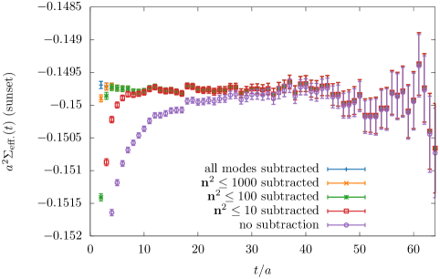
Figure 5: Sunset diagram (left diagram in fig. 1) contribution to the effective scalar self-energy eq. 144 with various excited-state subtractions. The chosen volume here is $64^{3}\times 128$ and the momentum is $\mathbf{p}=\frac{2\pi}{32a}(1,0,0)$. The subtractions are done using the spectral representation in eq. 196 and a cutoff on the integer modes $\mathbf{n}=\frac{L}{2\pi}\mathbf{k}$.

V.3.4 Signal-to-noise ratios in single-particle correlation functions

The general results obtained by Parisi (Parisi, 1984) and Lepage (Lepage, 1989) regarding the behavior of signal-to-noise (StN) ratios in QCD correlation functions have been studied extensively, and are known to correctly predict the behavior of the StN in (multi-)baryon correlation functions, as detailed in e.g. , Refs. (Beane et al., 2009a, b). They are expected to apply with equivalent validity to the lattice QED correlation functions given in eq. 133. At late times, these correlation functions are expected to behave as

$$C(t,{\bf p})\rightarrow Z_{1}\ e^{-\omega({\bf p})t}\ +\ Z_{3}\ e^{-\omega_{3}({\bf p})t}\ +\ \cdots\,,$$ (146)

where $\omega_{3}$ is the energy of three particles carrying a total momentum ${\bf p}$, the ellipses denote contributions from higher energy states, including those with photons, and the $Z_{i}$ are overlap coefficients onto the state $i$. The “noise” function is defined as the square root of the (connected) variance correlation function which has late-time behavior

$$C_{\sigma^{2}}(t,{\bf p})\rightarrow Z_{\sigma^{2};0}\ e^{-2\omega({\bf 0})t}\ +\ Z_{\sigma^{2};j}\ e^{-2\omega^{\prime}_{j}({\bf 0})t}\ +\ \cdots\,,$$ (147)

where the interpolating operator has a non-zero overlap onto a pair of particles at rest. Here, electromagnetic shifts in the energies of multi-particle states have been neglected. The energy $\omega^{\prime}_{j}$ appearing in eq. 147 is that of the $j^{\rm th}$ excited state without disconnected contributions. In the absence of interactions, the only state contributing to the noise correlation function is one with back-to-back particles with momenta $\pm{\bf p}$. The StN ratios for single-particle correlation functions are expected to degrade at late times as

$$C(t,{\bf p})/\sqrt{C_{\sigma^{2}}(t,{\bf p})}\rightarrow\widetilde{Z}_{1}\ e^{-\omega_{StN}({\bf p})t}\ +\ \cdots\,,$$ (148)

where the StN energy scale appearing in the argument of the exponential is given by

$$\omega_{StN}({\bf p})\ =\ \omega({\bf p})\ -\ \omega({\bf 0})\,,$$ (149)

while being approximately independent of time at early times.

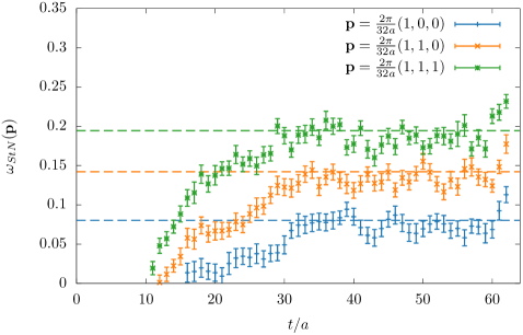
Figure 6: The energy scale, $\omega_{StN}({\bf p})$, associated with the StN ratio, given in eq. 149, calculated using the $32^{3}\times 128$ ensemble. The points and uncertainties result from correlation functions of particles with boosts ${\bf p}=\frac{2\pi}{32a}\mathbf{n}$ with $\mathbf{n}=(1,0,0)$, $\mathbf{n}=(1,1,0)$, and $\mathbf{n}=(1,1,1)$. The dashed lines correspond to $\omega(\mathbf{p})-\omega(\mathbf{0})$ for these momenta.

The results displayed in fig. 6 show that the Parisi-Lepage expressions (dashed horizontal lines) reproduce the late-time behavior of our results within uncertainties.

Generalizing to higher moments of the correlation functions, as has been done previously for multi-baryon correlation functions (Beane et al., 2015), the $n^{\rm th}$-even moments of the correlation functions can be argued to scale as $\sim e^{-n\omega({\bf 0})t}$ at late times, while the $(n+1)^{\rm th}$-odd moments scale as $\sim e^{-\omega_{n+1}({\bf p})t}$, where $\omega_{n+1}({\bf p})$ is the minimum energy of $n+1$ $\phi$’s carrying momentum ${\bf p}$. Consequently, at late times, the boosted single-particle correlation functions are expected to become symmetric and non-Gaussian.

V.3.5 Finite-volume scaling

In this section, the results of our scalar QED simulations are compared against the analytical finite-volume effects determined in section III. Specifically, the scalar self-energy on the lattice was computed for several different spatial volumes at fixed physical momenta. The infinite volume self-energy, calculated in lattice perturbation theory, was subtracted from the lattice results and compared with the analytical results given in eqs. 54 and 57.

For on-shell momenta, the volume scaling is shown for the rest frame in fig. 7, and for a selection of moving frames in fig. 8. The lattice results are seen to agree with the analytical results, except for small discrepancies at smaller volumes, which are of $\operatorname{\mathcal{O}}\left(e^{-mL}\right)$ and can therefore be attributed to exponential effects neglected in the analytical calculation. By numerically reproducing representative data points in lattice perturbation theory in a finite volume, we have indeed confirmed that this discrepancy is related to the neglected higher-order, exponentially suppressed finite-volume effects in our finite-volume expansion. For $\mathbf{p}=\frac{2\pi}{16a}(1,0,0)$ or larger, the poor StN ratio does not allow a reliable extraction of the on-shell self-energy. The volume scaling for a selection of off-shell momenta is shown in fig. 9. Again, good agreement is found between numerical and analytical calculations up to exponential corrections.

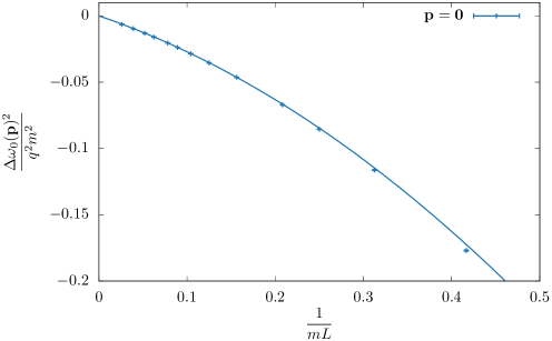
Figure 7: Volume scaling of the scalar on-shell self-energy in the rest frame. The points, and small associated uncertainties, come from the lattice scalar $\mathrm{QED}_{\mathrm{L}}$ simulations described in section V and the line corresponds to the analytical prediction eq. 54.

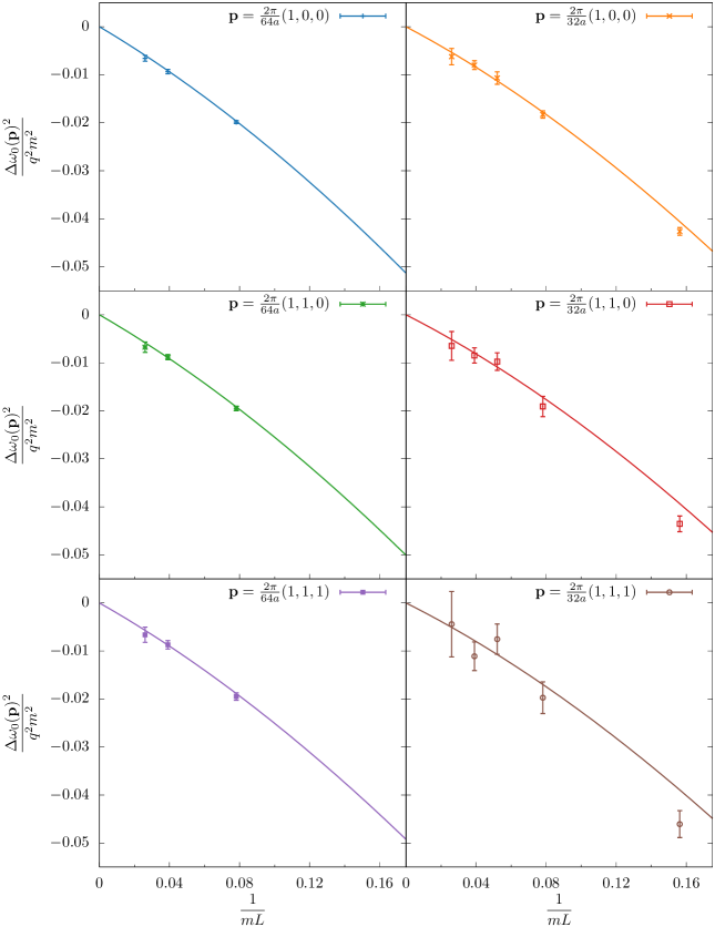
Figure 8: Volume scaling of the scalar on-shell self-energy for momenta of various directions and magnitudes. Other details are identical to fig. 7.

Figure 9: Volume scaling of the scalar self-energy for off-shell momenta with various orientations. The points come from the lattice scalar $\mathrm{QED}_{\mathrm{L}}$ simulations described in section V and the line corresponds to the analytical prediction eq. 57.

V.3.6 Infrared improvement

The method of infrared improvement, described in section IV, was implemented in our numerical calculation. Improved gauge ensembles of 100 configurations were generated for each of the volumes, and for each choice of the improvement weights given in table 2. The rest-frame scalar self energy has been calculated on these improved ensembles, and checked through exact analytical calculations of the difference in self-energy with and without improvement.

The upper panel of fig. 4 is reproduced in fig. 10, including the numerical values of finite-volume corrections to the mass of the scalar particle from the lattice simulations. The volume scaling from the improved ensembles behaves according to the analytical predictions, up to small deviations which can be attributed to exponential corrections that have been neglected in the analytical calculation. The discrepancy between numerical and analytical results is significantly smaller without improvement than with improvement, which we checked explicitly for representative data points. It appears that there is a suppression of exponential corrections that is broken by the improvement procedure.

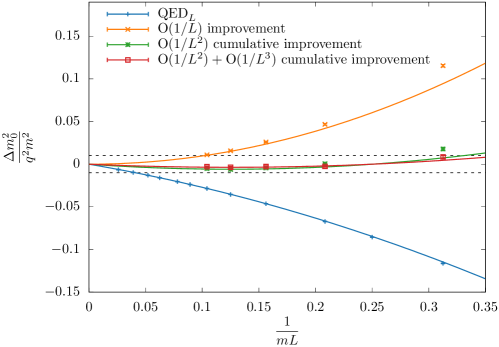
Figure 10: Relative finite-volume contributions to the mass squared of the scalar particle in $\mathrm{QED}_{\mathrm{L}}$, and the improved versions described in section IV. The points correspond to lattice scalar $\mathrm{QED}$ simulations described in section V, and with photon actions improved using the method described in section IV. The lines are the analytical predictions shown in the upper panel of fig. 4. The dashed line indicate the region within which the finite-volume contributions are below a percent of the electromagnetic corrections to the mass.

VI Low-Energy Effective Field Theories

The finite-volume modifications to the properties of charged particles in a lattice volume can be described by low-energy effective field theories. Calculations of the finite-volume mass of fundamental and composite charged scalars and fermions in non-relativistic QED (NRQED) (Lepage and Thacker, 1988; Thacker and Lepage, 1991; Hill et al., 2013) were performed by two of the authors (Davoudi and Savage, 2014). Finite-volume corrections to the mass calculated with NRQED were found to be in agreement with those of QED for scalar particles at leading order in $\alpha$, while a discrepancy was found between QED and NRQED for fermions at $\operatorname{\mathcal{O}}(1/L^{3})$ (Fodor et al., 2016b). This discrepancy is disturbing and has generated a number of subsequent investigations, e.g. Ref. (Fodor et al., 2016b; Lee and Tiburzi, 2016). In this section, we show why the NRQED calculations of the $\alpha/L^{3}$ finite-volume contribution to the mass of a charged fermion in Ref. (Davoudi and Savage, 2014) was incomplete, and explain why a residual mass term must be included in the NRQED Lagrange density to recover the correct low-energy QED result. We also extend these calculations to the self-energy of charged scalars and fermions carrying momentum. As the charged particles of interest can have arbitrary momentum in the rest frame of the lattice, NRQED does not provide an appropriate framework to calculate the low-energy properties of particles moving with a large momentum and effective field theories similar to Heavy-Quark Effective Field Theory (HQET) (Politzer and Wise, 1988; Georgi, 1990; Neubert, 1994; Manohar, 1997) and Heavy-Baryon Chiral Perturbation Theory (HB$\chi$PT) (Jenkins and Manohar, 1991a, b) are required.

VI.1 Heavy-Scalar QED

Heavy-Scalar QED (HSQED) is the EFT describing the low-momentum interactions of a charged scalar field, $\phi$, with the electromagnetic field after removing the momentum associated with its classical trajectory. The HSQED Lagrange density is in Minkowski space-time by

$${\cal L}[\phi]=\phi_{u}^{\dagger}iu\cdot D\phi_{u}-{1\over 2m_{\phi}}\phi_{u}^{\dagger}D_{\perp}^{2}\phi_{u}-\delta m_{\phi,u}\ \phi_{u}^{\dagger}\phi_{u}\,,$$ (150)

where $D_{\mu}=\partial_{\mu}+iqA_{\mu}$, and where the field has been redefined into the non-relativistic convention $\phi_{u}\rightarrow\phi_{u}/\sqrt{2m_{\phi}}$, and $\delta m_{\phi,u}$ is a residual mass. The full four-momentum of $\phi$ is $p=m_{\phi}u+k$, where $u^{2}=u_{0}^{2}-|{\bf u}|^{2}=1$, and the phase associated with the classical trajectory of $\phi$ in infinite volume has been removed, $\phi(x)=e^{-im_{\phi}u\cdot x}\phi_{u}(x)$, leaving a residual momentum $k$. $D_{\perp}^{\mu}=D^{\mu}-u^{\mu}u\cdot D$ where the equations of motion (Politzer, 1980) have been used. The components of the four-velocity are related to ${\bf v}$ by $u=\gamma(|\mathbf{v}|)(1,\mathbf{v})$. The dynamics of the electromagnetic field, $A_{\mu}(x)$, with the spatial zero mode removed are detailed in section II. The appearance of a residual mass term, $\delta m_{\phi,u}$, is at the heart of the present discussion and concerns the discrepancy between previous calculations (Davoudi and Savage, 2014; Fodor et al., 2016b). Removing the classical trajectory associated with the infinite-volume mass, $m_{\phi}$, through the aforementioned phase redefinition, leads to a vanishing residual mass in infinite volume. However, as we shall show through matching to the result of the full theory (scalar QED), in finite volume this term is non-vanishing at $\operatorname{\mathcal{O}}(1/L^{3})$ due to the removal of the spatial zero mode of $A_{\mu}(x)$. Calculations of the finite-volume contributions to the on-shell self energy up to NNLO in HSQED give

$$\Delta\Sigma_{0}^{\rm HSEFT}(p)_{|\sigma=0}=q^{2}\left\{\omega(\mathbf{p})(1-|\mathbf{v}|^{2})\frac{c_{2,1}(\mathbf{v})}{4\pi^{2}L}+\frac{c_{1}}{2\pi L^{2}}-\frac{|\mathbf{v}|^{2}}{4\omega(\mathbf{p})L^{3}}\right\}+2m_{\phi}\delta m_{\phi,u}\,.$$ (151)

The LO and NLO terms agree with the results in the full theory, but the NNLO loop contributions differ by a factor of two. As a result, matching the full and effective theories determines the residual mass to be

$$\delta m_{\phi,u}=-\frac{q^{2}|\mathbf{v}|^{2}}{8m_{\phi}\omega(\mathbf{p})L^{3}}=-\frac{q^{2}|\mathbf{v}|^{2}}{8\gamma(|\mathbf{v}|)\mu^{3}}m_{\phi}\,.$$ (152)

The residual mass vanishes in the rest frame, in agreement with previous calculations, but there is a non-zero residual mass for moving charged scalars that scales as $\sim 1/L^{3}$.

VI.2 Heavy-Fermion QED

The construction of the Heavy-Fermion QED (HFQED) follows along the same lines as for HSQED, but with the elimination of the lower components of the fermion spinor leaving a two-component theory. The field redefinitions can be found in previous literature, with the low-energy effective Lagrange density constructed to high orders in both the $1/m_{\psi}$ and coupling expansion, see e.g. Refs. (Manohar, 1997; Hill et al., 2013). The Lagrange density describing the low-energy dynamics of the charged fermion is known to be

$${\cal L}[\overline{\psi},\psi] =\overline{\psi}_{u}\left[iu\cdot D-\delta m_{\psi,u}-{1\over 2m_{\psi}}D_{\perp}^{2}-c_{F}\ {1\over 4m_{\psi}}\sigma_{\alpha\beta}F^{\alpha\beta}\right.$$

$$\qquad\quad\left.-c_{D}{1\over 8m_{\psi}^{2}}u^{\alpha}(D_{\perp}^{\beta}F_{\alpha\beta})+ic_{S}\ {1\over 8m_{\psi}^{2}}u_{\lambda}\sigma_{\alpha\beta}\{D_{\perp}^{\alpha},F^{\lambda\beta}\}\right]\psi_{u}\,,$$ (153)

where the coefficients of the operators, obtained by matching to infinite-volume QED, are $c_{F}=c_{D}=c_{S}=q$ at tree level, in which limit the residual mass $\delta m_{\psi,u}$ vanishes.

Calculation of the finite-volume contribution to the fermion self-energy with HFQED gives

$$\Delta\Sigma_{\frac{1}{2}}(p)_{|\sigma=0} =q^{2}\left\{\frac{m_{\psi}c_{2,1}(\mathbf{v})}{8\pi^{2}\omega(\mathbf{p})L}+\frac{c_{1}}{4\pi m_{\psi}L^{2}}+\frac{2\omega(\mathbf{p})^{2}+m_{\psi}^{2}}{8m_{\psi}\omega(\mathbf{p})^{3}L^{3}}\right\}$$

$$\quad+\frac{1}{8m_{\psi}\omega(\mathbf{p})L^{3}}\left(2c_{F}^{2}+qc_{D}-3q^{2}\right)+\delta m_{\psi,u}\,,$$ (154)

where the second to last term vanishes with the tree-level matching conditions. In order to recover the self-energy calculated in $\mathrm{QED}_{\mathrm{L}}$, given in eq. 65,

$$\delta m_{\psi,u}=q^{2}\frac{2\omega(\mathbf{p})^{2}+m_{\psi}^{2}}{8m_{\psi}\omega(\mathbf{p})^{3}L^{3}}=\frac{q^{2}(1+2\gamma(|\mathbf{v}|)^{2})}{8\gamma(|\mathbf{v}|)^{2}\mu^{3}}m_{\psi}.$$ (155)

The residual mass contribution adds to the loop contribution in HFQED to recover the $\operatorname{\mathcal{O}}(1/L^{3})$ contribution calculated with QED, by construction. Unlike the case of the charged scalar particle, the residual mass associated with a charged fermion does not vanish in the rest frame and its omission is seen to be responsible for the discrepancy in previous calculations (Davoudi and Savage, 2014; Fodor et al., 2016b).

It has been previously argued that contact interactions between fermions and anti-fermions need to be included in the low-energy EFT in order to recover the correct finite-volume QED mass shift at this order (Fodor et al., 2016b). In the rest frame, such interactions give rise to a contribution to the self-energy at this order, enabling NRQED to reproduce QED without the need for a residual mass term. One interpretation is that one must include anti-particles with a mass of $\gamma=2m_{\psi}$ into the theory and contract the anti-particle operators to recover this result. This is a somewhat unappealing feature of a low-energy EFT as this introduces a mass scale of $2m_{\psi}$ into the theory, and provides a dynamical ultraviolet scale in loop integrals that obscure an order-by-order power counting. The length scale of the anti-particle fluctuations is $1/(2m_{\psi})$, and through their interactions with the background charge density in $J_{\mu}(x)-{1\over L^{3}}\int_{\mathbb{T}^{3}}d^{3}{\bf y}\ J_{\mu}(t,{\bf y})$, give rise to a self-energy contribution of the form $1/(m_{\psi}^{2}L^{3})$. This makes clear that the separation between ultraviolet and infrared lengths scales, that is explicit in the construction of low-energy EFTs (particularly in matching to the full theory), is explicitly violated by removing a spatial mode of the electromagnetic field. In particular, the infinite-volume matching conditions between QED and the low-energy EFTs should be modified by contributions of the form $1/(m_{\psi}^{3}L^{3})$, which is found to be the case. As such contributions arise from physics at the length scale set by $1/(2m_{\psi})$, they can be included in the EFT through local counterterms as long as such length scales are not probed in the EFT. The residual mass term in HFQED at this order in the $\alpha$ expansion eliminates the need for such interactions with anti-particles or with the background charge density. The physics described here is essentially the same as that presented in Ref. (Patella, 2017) in which the details of operator matching in $\lambda\phi^{4}$ theory was considered when the zero mode of the field was removed.

We argue that from the calculational standpoint, QED and Scalar-QED are easier to work with than HFQED and HSQED for fundamental particles given the non-trivial finite-volume matching conditions. We anticipate that QED will be the most effective framework to go to higher orders in the loop expansion and in the $1/L^{n}$ expansion. The complexity associated with the non-locality of QED in the absence of the electromagnetic spatial zero-mode, and its implications for matching between QED and low-energy EFTs, while apparently tractable, adds new features to the EFTs that seem to be overly cumbersome.

VI.3 Implications for Hadrons and Composite Systems

In light of what was presented in this section, it is natural to contemplate the implications for hadronic theories, particularly Chiral Perturbation Theory ($\chi$PT), HB$\chi$PT and nuclear EFTs. In these theories, contributions to observables that are non-analytic in the quark masses are uniquely recovered from quantum loops, while analytic contributions are generated by loops and local counterterms in the Lagrange density. In the finite-volume QED, the numerical values of all of the local counterterms are expected to be modified by contributions scaling as $1/(\Lambda_{\chi}^{3}L^{3})$ due to the interactions of the quarks with the background charge densities associated with the other quarks and themselves. This is the same underlying mechanism that generates a non-zero residual mass term in HSQED and HFQED. We conclude that, while $\chi$PT and other low-energy EFTs can be used to determine the leading finite-volume electromagnetic contributions, and used to extrapolate them away, addressing contributions that scale as $1/L^{3}$ or higher appears to be more challenging.

VII Summary, Conclusions and Outlook

High-precision studies of strongly interacting hadronic systems using the numerical technique of lattice QCD require that QED is also included as a dynamical quantum field theory. Such studies are critical to the success of several experimental efforts in both high-energy physics and nuclear physics, including programs to measure anomalous magnetic moment of the muon and CP-violating observables in the decay of select hadrons; investigations that aim to find new physics by revealing minuscule deviations from the Standard Model predictions. Recognizing the need to include QED, numerical technologies and theoretical frameworks have been developed in recent years with which to facilitate lattice QCD+QED calculations. Unlike QCD, in which the strong dynamics confine the color charges of quarks and gluons, leading to a mass gap in the spectrum of the theory, QED contains massless photons coupled to a conserved charge, which introduce additional complications into the implementation and analysis of lattice QCD+QED calculations. The complications are the consequence of restricting QED to a finite spatial volume, where the need to impose boundary conditions on the fields “collides” with the classical equations of motion, including Gauss’s law and Ampere’s law. Perhaps the simplest technique to deal with this problem is to eliminate the zero spatial momentum mode of the photon field, and numerically evaluate observables in the remaining non-local QED-like field theory, called $\mathrm{QED}_{\mathrm{L}}$. The penalties incurred for such a modification to QED include power-law volume corrections to observables and the loss of the standard lore for constructing low-energy effective field theories. The locality of theory is restored in the infinite-volume limit. While other local formulations, including introducing a small photon mass Endres et al. (2016); Bussone et al. (2018) or using other boundary conditions Polley (1993); Wiese (1992); Kronfeld and Wiese (1993, 1991); Lucini et al. (2016); Hansen et al. (2018a), exist to define QED in a finite volume, the success of $\mathrm{QED}_{\mathrm{L}}$ in recent precision hadron spectroscopy studies, such as in Ref. Borsanyi et al. (2015), appears promising, and motivated us to investigate further a number of key theoretical and numerical aspects of such a scheme, to clarify its limitations, and to introduce improvement schemes.

In particular, by focusing on the dynamics of a single fundamental charged particle in lattice QED calculations, this work:

• Extends previous work to systems that are moving in the spatial volume. A systematic approach is taken to obtain a power-series expansion that allows power-law finite-volume QED corrections to the self-energy function to be obtained at leading order in $\alpha$ and to all orders in $\frac{1}{L}$. This approach provides a suitable framework for generalizing the formalism to composite charged particles. Rotational symmetry breaking effects due to the motion of a charged particle in a cubic volume are identified at leading orders in the $\frac{1}{L}$ expansion and the associated three-dimensional integer sums are evaluated via an efficient procedure.

• Introduces a mode-weighting technique that systematically improves the infrared scaling of self-energy of both spin-0 and spin-$1/2$ particles, reducing the size of finite-volume corrections to the mass of hadrons at typical volumes used in current lattice QCD+QED calculations. The generality of the procedure and its potential advantage in future calculations are discussed.

• Verifies the theoretical results obtained for the case of a fundamental scalar particle through a dedicated numerical study. The purpose for high-precision in this study was to reveal any potential effect that may not have been accounted for within the theoretical finite-volume framework, and to understand their origin. For boosted systems, the density of finite-volume states near the single-particle mass shell increases with velocity, as well as with the lattice volume. In scalar QED, such excited-state contributions are calculated analytically at leading order in $\alpha$ and removed from the lattice correlation functions, such that an identification of the self-energy from earlier Euclidean times is possible. The origin of observed signal-to-noise in boosted correlators is discussed, and is found consistent with the discussion by Parisi (Parisi, 1984) and Lepage (Lepage, 1989).

• Resolves a discrepancy in the literature concerning the $1/L^{3}$ finite-volume contributions calculated with NRQED and QED. It is shown how to account for missing contributions in effective field theory through introducing a local operator, a residual mass term, whose coefficient can only be fixed by matching to the full theory, $\mathrm{QED}_{\mathrm{L}}$.

We anticipate that the ideas presented in this work, along with the detailed theoretical and numerical explorations of $\mathrm{QED}_{\mathrm{L}}$, will be beneficial in the development and analysis of future high-precision lattice QCD+QED calculations of quantities of importance to experiment.

Appendix A Derivation of the general finite-volume formula

This appendix provides the details of the calculation in section III.2.1. We start by computing explicitly the residues $r_{\gamma}(\mathbf{k},p)$ and $r_{m}(\mathbf{k},p)$ defined in eq. 37,

$$r_{\gamma}(\mathbf{k},p) =\frac{f((i|\mathbf{k}|,\mathbf{k}),p)}{2|\mathbf{k}|[(p_{0}-i|\mathbf{k}|)^{2}+\omega(\mathbf{p}-\mathbf{k})^{2}]}\,,$$ (156)

$$r_{m}(\mathbf{k},p) =\frac{f((p_{0}+i\omega(\mathbf{p}-\mathbf{k}),\mathbf{k}),p)}{2\omega(\mathbf{p}-\mathbf{k})\{[p_{0}+i\omega(\mathbf{p}-\mathbf{k})]^{2}+|\mathbf{k}|^{2}\}}\,.$$ (157)

For the photon-pole effect $\Delta_{\gamma}(p)$, the on-shell and off-shell cases must be distinguished. Indeed, in the former the denominator of eq. 156 has an extra singularity at $\mathbf{k}^{2}=0$

$$(p_{0}-i|\mathbf{k}|)^{2}+\omega(\mathbf{p}-\mathbf{k})^{2}=2\omega(\mathbf{p})|\mathbf{k}|(-i\sqrt{\sigma-1}-\mathbf{v}\cdot\hat{\mathbf{k}})+\sigma\omega(\mathbf{p})^{2}\,,$$ (158)

which is $\operatorname{\mathcal{O}}(|\mathbf{k}|)$ at $\sigma=0$. Therefore, with the on-shell momentum $p=p_{\mathrm{o.s.}}=(i\omega(\mathbf{p}),\mathbf{p})$,

$$r_{\gamma}(\mathbf{k},p_{\mathrm{o.s.}})=\frac{f((i|\mathbf{k}|,\mathbf{k}),p_{\mathrm{o.s.}})}{4|\mathbf{k}|^{2}\omega(\mathbf{p})(1-\mathbf{v}\cdot\hat{\mathbf{k}})}\,.$$ (159)

Power-law finite-volume effects can be generated by this expression in two ways: firstly through the singularity in the denominator at $\mathbf{k}^{2}=0$, and secondly because of the eventual lack of smoothness of the numerator through its dependence to $|\mathbf{k}|$. The expansion of $f((i|\mathbf{k}|,\mathbf{k}),p)$ given in eq. 41 leads to

$$\Delta_{\gamma}(p_{\mathrm{o.s.}})=\frac{f_{0}(p_{\mathrm{o.s.}})c_{2,1}(\mathbf{v})}{16\pi^{2}\omega(\mathbf{p})L}+\sum_{j=1}^{+\infty}\frac{\xi_{2-j,1,j}(p_{\mathrm{o.s.}})}{2^{4-j}\pi^{2-j}\omega(\mathbf{p})L^{1+j}}+\cdots\,.$$ (160)

In the off-shell case, the denominator in eq. 158 is not simply proportional to $|\mathbf{k}|$ but also has a constant term. Writing the geometric expansion

$$\frac{1}{2|\mathbf{k}|[(p_{0}-i|\mathbf{k}|)^{2}+\omega(\mathbf{p}-\mathbf{k})^{2}]}=\frac{1}{2\sigma\omega(\mathbf{p})^{2}|\mathbf{k}|}\sum_{j=0}^{+\infty}(-1)^{j}\left[\frac{2(-i\sqrt{\sigma-1}-\mathbf{v}\cdot\hat{\mathbf{k}})}{\sigma\omega(\mathbf{p})}\right]^{j}|\mathbf{k}|^{j}\,,$$ (161)

and multiplying by eq. 41 leads to

$$r_{\gamma}(\mathbf{k},p_{\mathrm{o.s.}})=\frac{1}{2\sigma\omega(\mathbf{p})^{2}}\sum_{j=0}^{+\infty}\left\{\sum_{r=0}^{j}\left[\frac{2(i\sqrt{\sigma-1}+\mathbf{v}\cdot\hat{\mathbf{k}})}{\sigma\omega(\mathbf{p})}\right]^{r}f_{j-r}(\hat{\mathbf{k}},p)\right\}|\mathbf{k}|^{j-1}\,.$$ (162)

This last expression is quite cumbersome, and at this stage it is more useful to simplify it further on a case-to-case basis. The resulting leading finite-volume effect is

$$\Delta_{\gamma}(p)=\frac{f_{0}(p)c_{1}}{4\pi\sigma\omega(\mathbf{p})^{2}L^{2}}+\left[-\frac{i\sqrt{\sigma-1}\,f_{0}(p)}{\sigma^{2}\omega(\mathbf{p})^{3}}+\frac{\xi_{0,0,1}(p)}{2\sigma\omega(\mathbf{p})^{2}}\right]\frac{1}{L^{3}}+\operatorname{\mathcal{O}}\left(\frac{1}{L^{4}}\right)\,.$$ (163)

Turning to the charged particle function $\Delta_{m}(p)$, as functions of $\mathbf{k}$, $\omega(\mathbf{p}-\mathbf{k})$ and $|\mathbf{k}|^{2}$ are analytic, and $r_{m}(\mathbf{k},p)$ does not have singularities in $\mathbf{k}$, including at the on-shell point $p_{0}=i\omega(\mathbf{p})$, $r_{m}(\mathbf{k},p)$ is an analytic function of $\mathbf{k}$ and

$$\Delta_{m}(p)=-\frac{r_{m}(\mathbf{0},p)}{L^{3}}+\cdots=-\frac{f(((i+\sqrt{\sigma-1})\omega(\mathbf{p}),\mathbf{0}),p)}{2(i+\sqrt{\sigma-1})^{2}\omega(\mathbf{p})^{3}L^{3}}+\cdots\,,$$ (164)

where ellipsis denote exponentially suppressed finite-volume effects. Thus, this residue from the massive particle-pole only contributes a $\operatorname{\mathcal{O}}(\frac{1}{L^{3}})$ finite-volume effect coming from the zero-mode subtraction. It is worth nothing that there is an arbitrariness in our choice of the sign of $p_{0}$ at the on-shell point in Euclidean spacetime. While contributions from the photon and the particle pole in eqs. 163 and 164 are dependent upon this choice, the final result for the on-shell self energy, eqs. 54 and 65, is insensitive to such an arbitrariness.

Appendix B Numerical computation of the finite-volume coefficients

In this appendix, we discuss the numerical computation of the finite-volume coefficients $c_{j,k}(\mathbf{v})$ defined by eq. 42, that we recall here for convenience:

$$c_{j,k}(\mathbf{v})=\Delta_{\mathbf{n}}^{\prime}\left[\frac{1}{|\mathbf{n}|^{j}(1-\mathbf{v}\cdot\hat{\mathbf{n}})^{k}}\right]\,.$$ (165)

It is clear that $c_{j,k}(\mathbf{v})$ is finite only if $j<3$ because of the IR singularity at $|\mathbf{n}|=0$. Evaluating $c_{j,k}(\mathbf{v})$ numerically is a non-trivial task because it relies on cancellations between a sum and an integral which both diverge. One possible strategy, inspired by Refs. (Nijboer and Wette, 1957; Takahasi and Mori, 1973), is to introduce a damping function as follows:

$$c_{j,k}(\mathbf{v})=\Delta_{\mathbf{n}}^{\prime}\left[\frac{f(\eta\mathbf{n})}{|\mathbf{n}|^{j}(1-\mathbf{v}\cdot\hat{\mathbf{n}})^{k}}\right]+\Delta_{\mathbf{n}}^{\prime}\left[\frac{1-f(\eta\mathbf{n})}{|\mathbf{n}|^{j}(1-\mathbf{v}\cdot\hat{\mathbf{n}})^{k}}\right]\,,$$ (166)

where the function $f_{\eta}$ has the following properties:

1. $f(\mathbf{n})$ decays faster than any power of $|\mathbf{n}|$ at infinity.

2. $f(\eta\mathbf{n})$ converges to $1$ for $\eta\to 0$.

3. $|\mathbf{n}|^{-j}[1-f(\eta\mathbf{n})]$ is an infinitely differentiable function on $\mathbb{R}^{3}$.

The assumption (F1) guarantees that the first term in eq. 166 can be easily and cheaply evaluated numerically as the difference of rapidly converging sum and integral. Assumptions (F2) and (F3) guarantee, up to a constant, the second term in eq. 166 vanishes faster than any power of $\eta$ for $\eta\to 0$. In practice, one chooses a suitable function for $f$ and looks for a window where $\eta$ is small enough such that the second term in eq. 166 is negligible and does not have to be computed, while is still large enough to allow for a fast convergence of the first term.

Strongly inspired by Refs. (Tan, 2008; Takahasi and Mori, 1973), we choose the function

$$f(\mathbf{n})=1-\left(\tanh\{\sinh[|\mathbf{n}|(1-\mathbf{v}\cdot\hat{\mathbf{n}})^{\frac{k}{j+2}}]\}\right)^{j+2}\,.$$ (167)

for which it is straightforward to show that properties  (F1) and (F2) are satisfied. In fact, the decay rate of this function is doubly exponential (i.e. exponential of an exponential). However, the norm $|\mathbf{n}|$ is not differentiable on $\mathbb{R}^{3}$ so (F3) needs to be discussed further. One observes that $f$ has been crafted specifically so that $|\mathbf{n}|^{-j}(1-f(\eta\mathbf{n}))$ satisfies the following properties around the origin: firstly, it is non-singular in $|\mathbf{n}|$ and secondly it is even in $|\mathbf{n}|$. This ensures that $|\mathbf{n}|^{-j}(1-f(\eta\mathbf{n}))$ can be expanded in infinitely differentiable, even powers of $|\mathbf{n}|$ for $|\mathbf{n}|\to 0$, and therefore (F3) is true. More explicitly, the following Taylor expansion around the origin can be derived,

$$\frac{1-f(\eta\mathbf{n})}{|\mathbf{n}|^{j}(1-\mathbf{v}\cdot\hat{\mathbf{n}})^{k}}=\eta^{j+2}|\mathbf{n}|^{2}-\frac{j+2}{6}\eta^{j+4}(1-\mathbf{v}\cdot\hat{\mathbf{n}})^{\frac{2k}{j+2}}|\mathbf{n}|^{4}+\operatorname{\mathcal{O}}(|\mathbf{n}|^{6})\,.$$ (168)

Sketching the evaluation of $c_{j,k}(\mathbf{v})$ using this specific damping function, it is convenient to start by evaluating the the first term of eq. 166 as the difference between a convergent sum and an integral,

$$\Delta_{\mathbf{n}}^{\prime}\left[\frac{f(\eta\mathbf{n})}{|\mathbf{n}|^{j}(1-\mathbf{v}\cdot\hat{\mathbf{n}})^{k}}\right]=\operatorname*{\sideset{}{{}^{\prime}}{\sum}}_{\mathbf{n}}\frac{f(\eta\mathbf{n})}{|\mathbf{n}|^{j}(1-\mathbf{v}\cdot\hat{\mathbf{n}})^{k}}-\int\mathrm{d}^{3}\mathbf{n}\frac{f(\eta\mathbf{n})}{|\mathbf{n}|^{j}(1-\mathbf{v}\cdot\hat{\mathbf{n}})^{k}}\,.$$ (169)

Because of its doubly-exponential rate of convergence, the sum is trivial to evaluate numerically. The integral can be easily reduced to a one-dimensional integral,

$$\int\mathrm{d}^{3}\mathbf{n}\,\frac{f(\eta\mathbf{n})}{|\mathbf{n}|^{j}(1-\mathbf{v}\cdot\hat{\mathbf{n}})^{k}}=4\pi\eta^{j-3}R_{j}A_{\frac{5k}{j+2}}(|\mathbf{v}|)\,,$$ (170)

with

$$R_{j}=\int_{0}^{+\infty}\mathrm{d}r\,\frac{1-\tanh[\sinh(r)]^{j+2}}{r^{j-2}}\,,$$ (171)

and the function $A_{k}$ is defined in eq. 78. Using the expansion in eq. 168, it is clear that

$$\Delta_{\mathbf{n}}^{\prime}\left[\frac{1-f(\eta\mathbf{n})}{|\mathbf{n}|^{j}(1-\mathbf{v}\cdot\hat{\mathbf{n}})^{k}}\right]=0+\cdots\,,$$ (172)

where the ellipsis represents corrections that vanish exponentially fast as $\eta\to 0$.

Finally, $c_{j,k}(\mathbf{v})$ can be written as

$$c_{j,k}(\mathbf{v})=\operatorname*{\sideset{}{{}^{\prime}}{\sum}}_{\mathbf{n}}\frac{f(\eta\mathbf{n})}{|\mathbf{n}|^{j}(1-\mathbf{v}\cdot\hat{\mathbf{n}})^{k}}-4\pi\eta^{j-3}R_{j}A_{\frac{5k}{j+2}}(|\mathbf{v}|)+\cdots\,,$$ (173)

where only the sum and $R_{j}$ have to be evaluated numerically, both of which are straightforward tasks given their doubly-exponential convergence rate.

Appendix C Velocity suppression of the harmonic coefficients $a_{klm}(\mathbf{v})$

In this appendix, we prove that the harmonic coefficient $a_{klm}(\mathbf{v})$ in eq. 73 is an $\mathcal{O}(|\mathbf{v}|^{l})$ quantity. These coefficients are defined by

$$a_{klm}(\mathbf{v})=\int_{\mathrm{S}^{2}}\mathrm{d}^{2}\hat{\mathbf{n}}\,\frac{Y_{lm}(\theta_{\mathbf{n}},\phi_{\mathbf{n}})^{*}}{(1-\mathbf{v}\cdot\hat{\mathbf{n}})^{k}}\,.$$ (174)

The denominator of the integrand can be written as the power series

$$\frac{1}{(1-\mathbf{v}\cdot\hat{\mathbf{n}})^{k}}=\sum_{r=0}^{+\infty}\binom{k-1+r}{k-1}(\hat{\mathbf{v}}\cdot\hat{\mathbf{n}})^{r}|\mathbf{v}|^{r},$$ (175)

where the $\binom{n}{k}$ are the binomial coefficients. Further, $(\hat{\mathbf{v}}\cdot\hat{\mathbf{n}})^{r}$ can be written in the Legendre polynomial basis

$$(\hat{\mathbf{v}}\cdot\hat{\mathbf{n}})^{r}=\sum_{s=0}^{r}p_{rs}P_{s}(\hat{\mathbf{v}}\cdot\hat{\mathbf{n}})\,,$$ (176)

where it is known that (Weisstein, )

$$p_{rs}=\begin{cases}\displaystyle\frac{(2s+1)r!}{2^{\frac{r-s}{2}}(\frac{r-s}{2})!(r+s+1)!!}&\text{if }r\geq s\text{ and }r\equiv s\leavevmode\nobreak\ (\mathrm{mod}\leavevmode\nobreak\ 2),\\ 0&\text{otherwise.}\end{cases}$$ (177)

Using the spherical harmonics addition theorem

$$P_{s}(\hat{\mathbf{v}}\cdot\hat{\mathbf{n}})=\frac{4\pi}{2s+1}\sum_{t=-s}^{s}Y_{st}(\theta_{\mathbf{n}},\phi_{\mathbf{n}})Y_{st}(\theta_{\mathbf{v}},\phi_{\mathbf{v}})^{*}\,,$$ (178)

and the orthonormality of spherical harmonics, one obtains

$$\int_{\mathrm{S}^{2}}\mathrm{d}^{2}\hat{\mathbf{n}}\,(\hat{\mathbf{v}}\cdot\hat{\mathbf{n}})^{r}Y_{lm}(\theta_{\mathbf{n}},\phi_{\mathbf{n}})^{*}=\begin{cases}\displaystyle\frac{4\pi}{2l+1}p_{rl}Y_{lm}(\theta_{\mathbf{v}},\phi_{\mathbf{v}})^{*}&\text{if }l\leq r\\ 0&\text{otherwise.}\end{cases}$$ (179)

Finally, using this last result with eqs. 174 and 175, the following power-series representation of $a_{klm}(\mathbf{v})$ is obtained

$$a_{klm}(\mathbf{v})=\frac{4\pi}{2l+1}Y_{lm}(\theta_{\mathbf{v}},\phi_{\mathbf{v}})^{*}\sum_{r=l}^{+\infty}\binom{k-1+r}{k-1}p_{rl}|\mathbf{v}|^{r}\,.$$ (180)

This demonstrates that the rotational symmetry breaking effects with multipole index $l$ are suppressed by a factor $|\mathbf{v}|^{l}$, and explains why the $c_{j,k}(\mathbf{v})$ coefficients are essentially equal to the symmetric result at low velocities.

Appendix D Time-momentum representation of lattice scalar correlators

The time-momentum representation of the self-energy function that was derived in the continuum in eqs. 140 and 141 is extended to a self-energy function defined on a cubic lattice. Here, the time extent is assumed to be infinite while the spatial extent along each Cartesian coordinate is finite and has length $L$. We start by the following definition of various lattice versions of the energy and momentum

$$\hat{p}_{\mu} =\frac{2}{a}\sin\left(\frac{ap_{\mu}}{2}\right)\,,$$ (181)

$$\omega(\hat{\mathbf{p}}) =\sqrt{\hat{\mathbf{p}}^{2}+m^{2}}\,,$$ (182)

$$\omega_{\gamma}(\hat{\mathbf{k}}) =|\hat{\mathbf{k}}|\,,$$ (183)

$$\hat{\omega}(\mathbf{p}) =\frac{2}{a}\operatorname{arcsinh}\left[\frac{a\omega(\hat{\mathbf{p}})}{2}\right]\,,$$ (184)

$$\overline{\omega}(\mathbf{p}) =\frac{1}{a}\sinh\left[a\hat{\omega}(\mathbf{p})\right]=\omega(\hat{\mathbf{p}})\sqrt{1+\left(\frac{a\omega(\hat{\mathbf{p}})}{2}\right)^{2}}\,.$$ (185)

The scalar time-momentum correlator is defined as

$$C\left(t,\mathbf{p}\right)=C_{0}\left(t,\mathbf{p}\right)+C_{1}\left(t,\mathbf{p}\right)\,,$$ (186)

where $C_{0}\left(t,\mathbf{p}\right)$ is the free lattice scalar correlator

$$C_{0}\left(t,\mathbf{p}\right)=\int_{-\frac{\pi}{a}}^{\frac{\pi}{a}}\frac{dp_{0}}{2\pi}\frac{e^{ip_{0}t}}{\hat{p}_{0}^{2}+\omega(\hat{\mathbf{p}})^{2}}=\frac{e^{-\hat{\omega}(\mathbf{p})|t|}}{2\overline{\omega}(\mathbf{p})}\,,$$ (187)

and the self-energy $\Sigma(p)$ is given through the amputated first-order corrections

$$C_{1}\left(t,\mathbf{p}\right)=\int_{-\frac{\pi}{a}}^{\frac{\pi}{a}}\frac{dp_{0}}{2\pi}\frac{\Sigma\left(p\right)}{\left(\hat{p}^{2}+m^{2}\right)^{2}}e^{ip_{0}t}\,,$$ (188)

with

$$\Sigma\left(p\right)=\frac{q^{2}}{L^{3}}\operatorname*{\sideset{}{{}^{\prime}}{\sum}}_{\mathbf{k}\in\hat{\Lambda}^{3}}\int_{-\frac{\pi}{a}}^{\frac{\pi}{a}}\frac{dk_{0}}{2\pi}\left\{\frac{4-\frac{a^{2}}{2}\hat{p}^{2}}{\hat{k}^{2}}-\frac{(\widehat{2p-k})^{2}}{\hat{k}^{2}\left[(\widehat{p-k})^{2}+m^{2}\right]}\right\}\,.$$ (189)

The $k_{0}$ integral can be performed to give

$$\Sigma(p)=\frac{q^{2}}{L^{3}}\operatorname*{\sideset{}{{}^{\prime}}{\sum}}_{\mathbf{k}\in\hat{\Lambda}^{3}} \left\{\frac{2-\frac{a^{2}}{4}\hat{p}^{2}}{\overline{\omega}_{\gamma}(\mathbf{k})}-\frac{\frac{4}{a^{2}}\sin[ap_{0}-\frac{ia}{2}\hat{\omega}_{\gamma}(\mathbf{k})]^{2}+(\widehat{2\mathbf{p}-\mathbf{k}})^{2}}{2\overline{\omega}_{\gamma}(\mathbf{k})[\frac{4}{a^{2}}\sin(\frac{a}{2}p_{0}-\frac{ia}{2}\hat{\omega}_{\gamma}(\mathbf{k}))^{2}+\omega(\widehat{\mathbf{p}-\mathbf{k}})^{2}]}\right.$$

$$\quad\left.-\frac{\frac{4}{a^{2}}\sin[\frac{a}{2}p_{0}-\frac{ia}{2}\hat{\omega}(\mathbf{p}-\mathbf{k})]^{2}+(\widehat{2\mathbf{p}-\mathbf{k}})^{2}}{2\overline{\omega}(\mathbf{p}-\mathbf{k})[\frac{4}{a^{2}}\sin(\frac{a}{2}p_{0}+\frac{ia}{2}\hat{\omega}(\mathbf{p}-\mathbf{k}))^{2}+|\hat{\mathbf{k}}|^{2}]}\right\}\,.$$ (190)

The terms in the last expression have poles in the upper plane at the scalar-photon two-particle energy $p_{0}=i\hat{\omega}_{\gamma}(\mathbf{p},\mathbf{k})=i\hat{\omega}_{\gamma}(\mathbf{k})+i\hat{\omega}(\mathbf{p}-\mathbf{k})$. Note that analogous to the continuum case in eq. 190, $p_{0}=\pm i[\hat{\omega}_{\gamma}(\mathbf{k})-\hat{\omega}(\mathbf{p}-\mathbf{k})]$ is a removable singularity of the function (i.e. it is a pole with a vanishing residue). One can now compute eq. 188 using the rectangular contour in $p_{0}$ described in fig. 11 to obtain

$$C_{1}(t,\mathbf{p})=C_{1,\Sigma}(t,\mathbf{p})+C_{1,\gamma}(t,\mathbf{p})\,,$$ (191)

where $C_{1,\Sigma}$ denotes the contribution from the double pole at $p_{0}=i\hat{\omega}(\mathbf{p})$ and $C_{1,\gamma}$ denotes the contributions from the single pole $p_{0}=i\omega_{\gamma}(\mathbf{p},\mathbf{k})$,

$$C_{1,\Sigma}(t,\mathbf{p}) =\frac{e^{-\hat{\omega}(\mathbf{p})|t|}}{4\overline{\omega}(\mathbf{p})^{3}}\left[\left(1+\frac{1}{2}a^{2}\omega(\hat{\mathbf{p}})^{2}+\overline{\omega}(\mathbf{p})|t|\right)\Sigma\left(p_{\mathrm{o.s.}}\right)-i\overline{\omega}\left(\mathbf{p}\right)\left.\frac{\partial\Sigma(p)}{\partial p_{0}}\right|_{p_{\mathrm{o.s.}}}\right]\,,$$ (192)

$$C_{1,\gamma}(t,\mathbf{p}) =\frac{q^{2}}{L^{3}}\operatorname*{\sideset{}{{}^{\prime}}{\sum}}_{\mathbf{k}\in\mathrm{BZ}(L)}A(\mathbf{p},\mathbf{k})e^{-\hat{\omega}_{\gamma}(\mathbf{p},\mathbf{k})|t|}\,,$$ (193)

where $p_{\mathrm{o.s.}}=(i\hat{\omega}(\mathbf{p}),\mathbf{p}$) is the on-shell momentum, recovering $\hat{p}_{\mathrm{o.s.}}^{2}=-m^{2}$, and $A(\mathbf{p},\mathbf{k})$ is the amplitude given by

$$A(\mathbf{p},\mathbf{k})=-\frac{(\widehat{2\mathbf{p}-\mathbf{k}})^{2}-\frac{4}{a^{2}}\sinh[a\hat{\omega}(\mathbf{p}-\mathbf{k})+\frac{a}{2}\hat{\omega}_{\gamma}(\mathbf{k})]^{2}}{4\overline{\omega}(\mathbf{p}-\mathbf{k})\overline{\omega}_{\gamma}(\mathbf{k})\{\frac{4}{a^{2}}\sinh[\frac{a}{2}\hat{\omega}_{\gamma}(\mathbf{p},\mathbf{k})]^{2}-\omega(\hat{\mathbf{p}})^{2}\}^{2}}\,.$$ (194)

Finally, an effective on-shell self-energy can be constructed from $C_{0}$ and $C_{1}$ correlators

$$\Sigma_{\mathrm{eff.}}(t,\mathbf{p}) =2q^{2}\overline{\omega}(\mathbf{p})\frac{\operatorname{sign}(t)}{a}\left[\frac{C_{1}\left(t+a,\mathbf{p}\right)}{C_{0}\left(t+a,\mathbf{p}\right)}-\frac{C_{1}\left(t,\mathbf{p}\right)}{C_{0}\left(t,\mathbf{p}\right)}\right]$$ (195)

$$\underset{|t|\to+\infty}{=}\Sigma(p_{\mathrm{o.s.}})\,.$$ (196)

It is straightforward to verify that these results recover the continuum results in section V.

Figure 11: Rectangular contour used in appendix D for computing the energy Fourier transform of lattice correlators. This is a contour in the $p_{0}$ band with $-\frac{\pi}{a}\leq\mathrm{Re}(p_{0})\leq\frac{\pi}{a}$. The integrals on the intervals $\Gamma_{+}$ and $\Gamma_{-}$ cancel by periodicity and the integral on $\Gamma_{\Lambda}$ decays exponentially fast when the cutoff $\Lambda$ goes to $+\infty$. The dots represent the poles contributing to the self-energy contribution eq. 192 and the crosses denote the scalar-photon scattering states contributing to eq. 193.

Appendix E Parameters used for fits of the lattice on-shell scalar self-energy

The parameters used in extracting the scalar self-energy from the results of the lattice calculations of this work, as described in eq. 145, are presented in tables 3 and 4.

$N_{L}$	$\frac{L}{2\pi}\mathbf{p}$	$\mathbf{n}_{\mathrm{max}}^{2}$	$N_{\mathrm{sub.}}$
$\leq 64$			$N_{L}^{3}-1$
80	(0,0,0)	128	6042
96	(0,0,0)	256	17076
96	(3,0,0)	256	17076
96	(3,3,0)	256	17076
96	(3,3,3)	512	48500
128	(0,0,0)	256	17076
128	(2,0,0)	512	48500
128	(2,2,0)	512	48500
128	(2,2,2)	512	48500
128	(4,0,0)	512	48500
128	(4,4,0)	512	48500
128	(4,4,4)	512	48500
192	(0,0,0)	512	48500
192	(3,0,0)	512	48500
192	(3,3,0)	1024	137064
192	(3,3,3)	1024	137064
192	(6,0,0)	1024	137064
192	(6,6,0)	1024	137064
192	(6,6,6)	1024	137064

Table 3: Number of excited states $N_{\mathrm{sub.}}$ subtracted from each scalar 2-point function. When applied, the cutoff imposed on the photon modes $\mathbf{n}_{\mathrm{max}}^{2}=\frac{L}{2\pi}\mathbf{k}_{\mathrm{max}}^{2}$ is given.

$N_{L}$	$\frac{L}{2\pi}\mathbf{p}$	$t_{\mathrm{min}}$	$t_{\mathrm{max}}$
12	(0,0,0)	3	57
16	(0,0,0)	3	57
20	(0,0,0)	3	60
24	(0,0,0)	3	62
32	(0,0,0)	3	61
32	(1,0,0)	3	29
32	(1,1,0)	3	17
32	(1,1,1)	3	10
40	(0,0,0)	3	58
48	(0,0,0)	3	58
56	(0,0,0)	3	61
64	(0,0,0)	3	48
64	(1,0,0)	3	48
64	(1,1,0)	3	48
64	(1,1,1)	3	40
64	(2,0,0)	3	26
64	(2,2,0)	3	26
64	(2,2,2)	3	14
80	(0,0,0)	3	53

$N_{L}$	$\frac{L}{2\pi}\mathbf{p}$	$t_{\mathrm{min}}$	$t_{\mathrm{max}}$
96	(0,0,0)	3	59
96	(3,0,0)	3	34
96	(3,3,0)	3	19
96	(3,3,3)	3	9
128	(0,0,0)	3	107
128	(2,0,0)	3	102
128	(2,2,0)	3	29
128	(2,2,2)	3	30
128	(4,0,0)	3	31
128	(4,4,0)	3	19
128	(4,4,4)	3	13
192	(0,0,0)	3	110
192	(3,0,0)	3	94
192	(3,3,0)	3	57
192	(3,3,3)	3	31
192	(6,0,0)	3	11
192	(6,6,0)	3	11
192	(6,6,6)	3	10

Table 4: Time intervals used for fits to effective on-shell self energies.

References

- Aoki et al. (2017) S. Aoki et al., Eur. Phys. J. C77, 112 (2017), arXiv:1607.00299 [hep-lat] .
- Duncan et al. (1996) A. Duncan, E. Eichten, and H. Thacker, Phys. Rev. Lett. 76, 3894 (1996), arXiv:hep-lat/9602005 [hep-lat] .
- Blum et al. (2007) T. Blum, T. Doi, M. Hayakawa, T. Izubuchi, and N. Yamada, Phys. Rev. D76, 114508 (2007), arXiv:0708.0484 [hep-lat] .
- Blum et al. (2010) T. Blum, R. Zhou, T. Doi, M. Hayakawa, T. Izubuchi, S. Uno, and N. Yamada (RBC-UKQCD), Phys. Rev. D82, 094508 (2010), arXiv:1006.1311 [hep-lat] .
- Ishikawa et al. (2012) T. Ishikawa, T. Blum, M. Hayakawa, T. Izubuchi, C. Jung, and R. Zhou, Phys. Rev. Lett. 109, 072002 (2012), arXiv:1202.6018 [hep-lat] .
- Aoki et al. (2012) S. Aoki et al., Phys. Rev. D86, 034507 (2012), arXiv:1205.2961 [hep-lat] .
- Borsanyi et al. (2013) S. Borsanyi et al. (BMWc), Phys. Rev. Lett. 111, 252001 (2013), arXiv:1306.2287 [hep-lat] .
- Borsanyi et al. (2015) S. Borsanyi et al. (BMWc), Science 347, 1452 (2015), arXiv:1406.4088 [hep-lat] .
- Portelli (2015) A. Portelli, Proceedings, 32nd International Symposium on Lattice Field Theory (Lattice 2014): Brookhaven, NY, USA, June 23-28, 2014, PoS LATTICE2014, 013 (2015), arXiv:1505.07057 [hep-lat] .
- Horsley et al. (2016a) R. Horsley et al., J. Phys. G43, 10LT02 (2016a), arXiv:1508.06401 [hep-lat] .
- Horsley et al. (2016b) R. Horsley et al., JHEP 04, 093 (2016b), arXiv:1509.00799 [hep-lat] .
- Fodor et al. (2016a) Z. Fodor, C. Hoelbling, S. Krieg, L. Lellouch, T. Lippert, A. Portelli, A. Sastre, K. K. Szabo, and L. Varnhorst (BMWc), Phys. Rev. Lett. 117, 082001 (2016a), arXiv:1604.07112 [hep-lat] .
- de Divitiis et al. (2013) G. M. de Divitiis, R. Frezzotti, V. Lubicz, G. Martinelli, R. Petronzio, G. C. Rossi, F. Sanfilippo, S. Simula, and N. Tantalo (RM123), Phys. Rev. D87, 114505 (2013), arXiv:1303.4896 [hep-lat] .
- Giusti et al. (2017a) D. Giusti, V. Lubicz, C. Tarantino, G. Martinelli, S. Sanfilippo, S. Simula, and N. Tantalo (RM123), Phys. Rev. D95, 114504 (2017a), arXiv:1704.06561 [hep-lat] .
- Basak et al. (2018) S. Basak et al. (MILC), (2018), arXiv:1807.05556 [hep-lat] .
- Hansen et al. (2018a) M. Hansen, B. Lucini, A. Patella, and N. Tantalo, JHEP 05, 146 (2018a), arXiv:1802.05474 [hep-lat] .
- Blum et al. (2017) T. Blum, N. Christ, M. Hayakawa, T. Izubuchi, L. Jin, C. Jung, and C. Lehner, Phys. Rev. D96, 034515 (2017), arXiv:1705.01067 [hep-lat] .
- Blum et al. (2018) T. Blum, P. A. Boyle, V. Gülpers, T. Izubuchi, L. Jin, C. Jung, A. Jüttner, C. Lehner, A. Portelli, and J. T. Tsang (RBC, UKQCD), Phys. Rev. Lett. 121, 022003 (2018), arXiv:1801.07224 [hep-lat] .
- Carrasco et al. (2015) N. Carrasco, V. Lubicz, G. Martinelli, C. T. Sachrajda, N. Tantalo, C. Tarantino, and M. Testa, Phys. Rev. D91, 074506 (2015), arXiv:1502.00257 [hep-lat] .
- Lubicz et al. (2017) V. Lubicz, G. Martinelli, C. T. Sachrajda, F. Sanfilippo, S. Simula, and N. Tantalo, Phys. Rev. D95, 034504 (2017), arXiv:1611.08497 [hep-lat] .
- Giusti et al. (2018) D. Giusti, V. Lubicz, G. Martinelli, C. T. Sachrajda, F. Sanfilippo, S. Simula, N. Tantalo, and C. Tarantino, Phys. Rev. Lett. 120, 072001 (2018), arXiv:1711.06537 [hep-lat] .
- Christ and Feng (2018) N. Christ and X. Feng, Proceedings, 35th International Symposium on Lattice Field Theory (Lattice 2017): Granada, Spain, June 18-24, 2017, EPJ Web Conf. 175, 13016 (2018), arXiv:1711.09339 [hep-lat] .
- Giusti et al. (2017b) D. Giusti, V. Lubicz, G. Martinelli, F. Sanfilippo, and S. Simula, JHEP 10, 157 (2017b), arXiv:1707.03019 [hep-lat] .
- Boyle et al. (2017) P. Boyle, V. Gülpers, J. Harrison, A. Jüttner, C. Lehner, A. Portelli, and C. T. Sachrajda, JHEP 09, 153 (2017), arXiv:1706.05293 [hep-lat] .
- Duncan et al. (1997) A. Duncan, E. Eichten, and H. Thacker, Phys. Lett. B409, 387 (1997), arXiv:hep-lat/9607032 [hep-lat] .
- Hayakawa and Uno (2008) M. Hayakawa and S. Uno, Prog. Theor. Phys. 120, 413 (2008), arXiv:0804.2044 [hep-ph] .
- Davoudi and Savage (2014) Z. Davoudi and M. J. Savage, Phys. Rev. D90, 054503 (2014), arXiv:1402.6741 [hep-lat] .
- Fodor et al. (2016b) Z. Fodor, C. Hoelbling, S. D. Katz, L. Lellouch, A. Portelli, K. K. Szabo, and B. C. Toth, Phys. Lett. B755, 245 (2016b), arXiv:1502.06921 [hep-lat] .
- Lee and Tiburzi (2016) J.-W. Lee and B. C. Tiburzi, Phys. Rev. D93, 034012 (2016), arXiv:1508.04165 [hep-lat] .
- Matzelle and Tiburzi (2017) M. E. Matzelle and B. C. Tiburzi, Phys. Rev. D95, 094510 (2017), arXiv:1702.01296 [hep-lat] .
- Endres et al. (2016) M. G. Endres, A. Shindler, B. C. Tiburzi, and A. Walker-Loud, Phys. Rev. Lett. 117, 072002 (2016), arXiv:1507.08916 [hep-lat] .
- Bussone et al. (2018) A. Bussone, M. Della Morte, and T. Janowski, Proceedings, 35th International Symposium on Lattice Field Theory (Lattice 2017): Granada, Spain, June 18-24, 2017, EPJ Web Conf. 175, 06005 (2018), arXiv:1710.06024 [hep-lat] .
- Polley (1993) L. Polley, Z. Phys. C59, 105 (1993).
- Wiese (1992) U. J. Wiese, Nucl. Phys. B375, 45 (1992).
- Kronfeld and Wiese (1993) A. S. Kronfeld and U. J. Wiese, Nucl. Phys. B401, 190 (1993), arXiv:hep-lat/9210008 [hep-lat] .
- Kronfeld and Wiese (1991) A. S. Kronfeld and U. J. Wiese, Nucl. Phys. B357, 521 (1991).
- Lucini et al. (2016) B. Lucini, A. Patella, A. Ramos, and N. Tantalo, JHEP 02, 076 (2016), arXiv:1509.01636 [hep-th] .
- Bijnens et al. (2018) J. Bijnens, J. Harrison, N. Hermansson-Truedsson, T. Janowski, A. Jüttner, and A. Portelli, To appear (2018).
- Faddeev and Popov (1967) L. D. Faddeev and V. N. Popov, Phys. Lett. 25B, 29 (1967).
- Hansen et al. (2018b) M. Hansen, B. Lucini, A. Patella, and N. Tantalo, Proceedings, 35th International Symposium on Lattice Field Theory (Lattice 2017): Granada, Spain, June 18-24, 2017, EPJ Web Conf. 175, 09001 (2018b), arXiv:1710.08838 [hep-lat] .
- Campos, Isabel and Fritzsch, Patrick and Hansen, Martin and Marinković, Marina Krstić and Patella, Agostino and Ramos, Alberto and Tantalo, Nazario (2018) Campos, Isabel and Fritzsch, Patrick and Hansen, Martin and Marinković, Marina Krstić and Patella, Agostino and Ramos, Alberto and Tantalo, Nazario, Proceedings, 35th International Symposium on Lattice Field Theory (Lattice 2017): Granada, Spain, June 18-24, 2017, EPJ Web Conf. 175, 09005 (2018), arXiv:1710.08839 [hep-lat] .
- Luscher (1986) M. Luscher, Commun. Math. Phys. 105, 153 (1986).
- Borwein et al. (2013) J. M. Borwein, M. L. Glasser, R. C. McPhedran, J. G. Wan, and I. J. Zucker, Lattice Sums Then and Now, Encyclopedia of Mathematics and its Applications (Cambridge University Press, 2013).
- Davoudi and Savage (2012) Z. Davoudi and M. J. Savage, Phys. Rev. D86, 054505 (2012), arXiv:1204.4146 [hep-lat] .
- Detmold and Lin (2006) W. Detmold and C. J. D. Lin, Phys. Rev. D73, 014501 (2006), arXiv:hep-lat/0507007 [hep-lat] .
- Monahan and Orginos (2015) C. Monahan and K. Orginos, Phys. Rev. D91, 074513 (2015), arXiv:1501.05348 [hep-lat] .
- Davoudi and Savage (2011) Z. Davoudi and M. J. Savage, Phys. Rev. D84, 114502 (2011), arXiv:1108.5371 [hep-lat] .
- Briceno et al. (2013) R. A. Briceno, Z. Davoudi, T. Luu, and M. J. Savage, Phys. Rev. D88, 114507 (2013), arXiv:1309.3556 [hep-lat] .
- Briceno et al. (2014) R. A. Briceno, Z. Davoudi, T. C. Luu, and M. J. Savage, Phys. Rev. D89, 074509 (2014), arXiv:1311.7686 [hep-lat] .
- Beane and Savage (2014) S. R. Beane and M. J. Savage, Phys. Rev. D90, 074511 (2014), arXiv:1407.4846 [hep-lat] .
- Boyle et al. (2016) P. A. Boyle, G. Cossu, A. Yamaguchi, and A. Portelli, Proceedings, 33rd International Symposium on Lattice Field Theory (Lattice 2015): Kobe, Japan, July 14-18, 2015, PoS LATTICE2015, 023 (2016).
- Parisi (1984) G. Parisi, COMMON TRENDS IN PARTICLE AND CONDENSED MATTER PHYSICS. PROCEEDINGS, WINTER ADVANCED STUDY INSTITUTE, LES HOUCHES, FRANCE, FEBRUARY 23 - MARCH 11, 1983, Phys. Rept. 103, 203 (1984).
- Lepage (1989) G. P. Lepage, in Boulder ASI 1989:97-120 (1989) pp. 97–120.
- Beane et al. (2009a) S. R. Beane, W. Detmold, T. C. Luu, K. Orginos, A. Parreno, M. J. Savage, A. Torok, and A. Walker-Loud, Phys. Rev. D79, 114502 (2009a), arXiv:0903.2990 [hep-lat] .
- Beane et al. (2009b) S. R. Beane, W. Detmold, T. C. Luu, K. Orginos, A. Parreno, M. J. Savage, A. Torok, and A. Walker-Loud, Phys. Rev. D80, 074501 (2009b), arXiv:0905.0466 [hep-lat] .
- Beane et al. (2015) S. R. Beane, W. Detmold, K. Orginos, and M. J. Savage, J. Phys. G42, 034022 (2015), arXiv:1410.2937 [nucl-th] .
- Lepage and Thacker (1988) G. P. Lepage and B. A. Thacker, FIELD THEORY ON THE LATTICE. PROCEEDINGS, INTERNATIONAL SYMPOSIUM, SEILLAC, FRANCE, SEPTEMBER 28 - OCTOBER 2, 1987, Nucl. Phys. Proc. Suppl. 4, 199 (1988).
- Thacker and Lepage (1991) B. A. Thacker and G. P. Lepage, Phys. Rev. D43, 196 (1991).
- Hill et al. (2013) R. J. Hill, G. Lee, G. Paz, and M. P. Solon, Phys. Rev. D87, 053017 (2013), arXiv:1212.4508 [hep-ph] .
- Politzer and Wise (1988) H. D. Politzer and M. B. Wise, Phys. Lett. B208, 504 (1988).
- Georgi (1990) H. Georgi, Phys. Lett. B240, 447 (1990).
- Neubert (1994) M. Neubert, Phys. Rept. 245, 259 (1994), arXiv:hep-ph/9306320 [hep-ph] .
- Manohar (1997) A. V. Manohar, Phys. Rev. D56, 230 (1997), arXiv:hep-ph/9701294 [hep-ph] .
- Jenkins and Manohar (1991a) E. E. Jenkins and A. V. Manohar, Phys. Lett. B255, 558 (1991a).
- Jenkins and Manohar (1991b) E. E. Jenkins and A. V. Manohar, in Workshop on Effective Field Theories of the Standard Model Dobogoko, Hungary, August 22-26, 1991 (1991) pp. 113–137.
- Politzer (1980) H. D. Politzer, Nucl. Phys. B172, 349 (1980).
- Patella (2017) A. Patella, Proceedings, 34th International Symposium on Lattice Field Theory (Lattice 2016): Southampton, UK, July 24-30, 2016, PoS LATTICE2016, 020 (2017), arXiv:1702.03857 [hep-lat] .
- Nijboer and Wette (1957) B. Nijboer and F. D. Wette, Physica 23, 309 (1957).
- Takahasi and Mori (1973) H. Takahasi and M. Mori, PRIMS 9, 721 (1973).
- Tan (2008) S. Tan, Phys. Rev. A78, 013636 (2008), arXiv:0709.2530 [cond-mat.stat-mech] .
- (71) E. W. Weisstein, “Legendre polynomial. From MathWorld—A Wolfram Web Resource,” Last visited on 30/08/2017.